Embed Size (px)
Citation preview

Pergamon Computers chem. Engng Vol. 21, No. 7, pp. 675-689, 1997
Copyright © 1997 Elsevier Science Ltd Printed in Great Britain. All fights reserved
PII: S0098-1354(96)00301-8 0098-1354/97 $17.00+0.00
Nonsmooth dynamic simulation with linear programming based methods
Vipin Gopal* and Lorenz T. Bieglert
Department of Chemical Engineering and Engineering Design Research Center, Carnegie Mellon University, Pittsburgh, PA 15213, U.S.A.
(Received 27 June 1995; revised 6 May 1996)
Abstract
Process simulation has emerged as a valuable tool for process design, analysis and operation. In this work, we extend the capabilities of iterated linear programming (LP) for dealing with problems encountered in dynamic nonsmooth process simulation. A previously developed LP method is refined with the addition of a new descent strategy which combines line search with a trust region approach. This adds more stability and efficiency to the method. The LP method has the advantage of naturally dealing with profile bounds as well. This is demonstrated to avoid the computational difficulties which arise from the iterates going into physically unrealistic regions. A new method for the treatment of discontinuities occurring in dynamic simulation problems is also presented in this paper. The method ensures that any event which has occurred within the time interval in consideration is detected and if more than one event occurs, the detected one is indeed the earliest one. A specific class of implicitly discontinuous process simulation problems, phase equilibrium calculations, is also examined. A new formulation is introduced to solve multiphase problems. © 1997 Elsevier Science Ltd. All rights reserved
Keywords: Nonsmooth simulation; Iterated linear programming; Line search; Trust region; Profile Bounds; Discontinuity
1. Introduction
Recent years have seen the emergence of process simulation as a valuable tool for plant design, analysis and operation. A variety of factors like increased safety concerns and strict environmental regulations have contributed to this trend. Of increasing interest in the simulation community is the development of efficient dynamic simulation tools. Many authors have surveyed the present and future applications of such tools in chemical process industries (Perkins, 1986; Marquardt, 1991; Naess et al., 1992; Pantelides and Barton, 1993).
Equation oriented simulators, as opposed to their sequential modular counterparts, rely on an equation solving engine which must be able to handle poor starting points, inequality constraints, singularities and ill-conditioning, among others. Steady state and dynamic chemical process simulation also invariably encounter variables which need to be restricted within certain bounds. Typical examples are the nonnegativity restric- tions on physical quantities like mass, volume or
* email: [email protected] t email: [email protected]
temperature. Process models could show abnormal behavior if these variables are allowed to take values beyond these bounds because of physical or mathemat- ical infeasibility. A systematic treatment of these bounds by the solver can avoid convergence failures which might arise due to ad hoc strategies currently employed.
Another important issue is the treatment of nonsmooth relations characterized by discontinuous derivatives or kinks, which are often enforced as procedures in the sequential modular mode. Bullard (1991) examined some of these problems in the context of steady state simulation. Marquardt (1991), on the other hand, points out that most of the current dynamic simulation packages are developed to solve models of predom- inantly continuous nature. However, few industrial processes could be considered to operate in a truly continuous manner. Simulation of dynamic chemical processes often involves discrete actions and logical constraints and these can lead to discontinuities in the modeling equations. Process models can thus be non- smooth at various points in state space, with these points specified through explicit or implicit relations. Typical examples of these include phase and flow transitions, heat and mass transfer correlations in various regimes
675

676 V. GOPAL and L. T. BIEGLER
and startup and shutdown operations in continuous plants. The discontinuity might cause either a switch in the model equations or even a change in the structure and dimensionality of the plant model. Hence an effective and consistent representation mechanism of the model discontinuities and their solution technique is very important in an equation based modeling environ- ment.
A method based on iterated linear programming is presented in this paper for the treatment of variable bounds and nonsmoothness occurring in process simula- tion problems. In the next section we look at a previously developed iterated linear programming tech- nique for constrained simulation problems modified with an improved descent strategy. The LP based method provides a very natural way of incorporating variable bounds. Other than bounds on variables, physically realistic conditions could also be added through simple inequalities. Section 3 focuses on the need for an efficient treatment of variable bounds and how the LP method provides a framework for the purpose. A new algorithm for the treatment of discontinuities occurring in dynamic simulation problems is presented in Section 4. Section 5 describes the treatment of implicit dis- continuities by looking at a specific class of problems: phase equilibrium calculations. Conclusions and future work are outlined in Section 6.
2. Improved iterated LP method for constrained simulation problems
Bullard and Biegler (1991) introduced a technique based on iterated linear programming for solving a nonlinear system of equations subject to inequality constraints and variable bounds.
h:(x)=O
gk(x)<-O
xL<x<--x U (CSP)
This problem is termed as the constrained simulation problem (CSP). The basic idea of the approach is to convert the equation solving problem to an optimization problem. A sequence of linear programs is then solved to yield search directions that wil l lead to the solution of the nonlinear problem.
To solve (CSP), a merit function is defined as
(1)
where gk(x~)+ = max [0, gk(x0]. Since /~ ~0 has a minimum of zero if and only if (CSP) is solved, p, a non differentiable function, is minimized subject to x L -< x -< x u. By adding auxiliary variables, this problem can be written as:
Min E (p:+nj)+ ~ s,
s.t. hj(x)=pj - nj
gk(X)<--Sk
xL<x~_X U
pj,nj,sk>--O (2)
Barrodale and Roberts (1978) proved that for Ej(pj + nj) at a minimum, a complementarity condition pin/ =0 holds. Thus (pj + nj) represents Ihj(x)l and s k represents &(x).. Linearizing the constraints about x ~ leads to the following constrained simulation linear program, CSLP:
Min E (pj+n~)+ E s,
s.t. hj(~)+ q hlOg)rd=pj - nj
&O?)+ V gk(.e)rd<--sk
XL<__~ +C~<_X u
pj,n~,sk>--O (CSLP)
The solution of (CSLP) generates a search direction d. To stabilize the performance of tl/e algorithm, a line search is carried out to find some fraction a so that x TM = x ~ + ad'. It should be noted that this method reduces to Newton's method in the absence of active inequality constraints and thus has the ability to converge quad- ratically to the solution. This LP approach is also shown to generate a descent direction for the 1-norm of the constraint violations. The method has global con- vergence properties for a nonzero solution of the linear program. The algorithm, when tested on problems ranging from 2 to 977 equations, compared favorably with the existing methods.
Here a new descent strategy is incorporated into the aforementioned algorithm by combining two major classes of strategies used to ensure descent: line search and trust region methods. Dennis and Schnabel (1983) and Fletcher (1987) provide a detailed study of these methods.
2.1. Line search methods
The basic concept behind using line search methods is to choose a descent direction d from the current point x j and select an acceptable point x ~+~ in this direction at which ~x) decreases. The implementation for the algorithm by Bullard and Biegler (1991) uses the traditional monotonic, Armijo-type line search (Armijo, 1966). The search direction d is obtained from the solution of (CSLP) and a condition (3) that requires a sufficient decrease in the merit function is enforced.
/z(x% ox/~) -/z(x~)--<0. I aDabr (3)
Here Ddz is an upper bound on the directional derivative of the merit function, which is given by
Dale= ~ Q)j+nj)+ ~ St- ~ Ihj(x/)l- ~ gk(x/)+ (4)
At the full step (a = 1), (3) is evaluated. If satisfied, the

Nonsmooth dynamic simulation
variables are updated and a new step is calculated. Otherwise a new fractional step (5) is calculated from a quadratic interpolation of the merit function and con- tinued until a suitable ot is found.
a=max{0 .1a , . - 0"5 a'2Dd z "~ ~(~e + , ~ ) - ~ ) - , ~ j (5)
Since the merit function is nondifferentiable, it is possible for the Maratos effect to occur (Fletcher, 1987). Here x ~ may be arbitrarily close to the solution x', but a full step may fail to reduce the merit function. A nonmonotonic line search such as the watchdog tech- nique (Chamberlein et al., 1982) or a second order correction (Fletcher, 1987) could be used to overcome this effect.
2.2. Trust region methods
Search directions generated by CSLP are always descent directions (Dd.¢ <0) for d ~0, but they still may be poor if the problem is ill-conditioned. In such cases, the search direction is relatively large and is nearly orthogonai to the steepest descent direction. Trust region methods avoid this problem by restricting the stepsize d to an area A i around the current point x( The trust region is frequently adjusted after each step depending on how valid the approximations to the model are. Most of the current implementations increase or decrease the trust region by comparing the actual reduction in the merit function and the predicted reduction on linearization. The closer their ratio is to unity, the better the agreement. Duff et al. (1987) describe this strategy in the context of using linear programs to solve sparse nonlinear equa-
tions.
2.3. A combination
The main difference between line search and trust region methods lies in the sequence in which they use the linear model and enforce the acceptable step length. The line search methods use a linear model to obtain a search direction d and then choose a fractional step a. Thus the line search occurs on a 1-dimensional sub- space. On the other hand, trust region methods first choose a maximum acceptable step length A and then use the linear model to obtain a search direction d, the length of which cannot exceed A. The search here is not restricted to a lower dimensional subspace. The trust region step may not always be in the Newton direction, particularly when A is small when compared to the Newton step. Instead, as A goes to zero, the LP direction becomes the closest vertex to the steepest descent direction. Since the trust region becomes inactive near the solution, both the Newton and LP-based method exhibit quadratic convergence near the solution.
Relatively little work is necessary for the line search method as only one LP is solved at each iteration. But, when trust region methods are used, finding the ideal trust region bounds is likely to require solution of more than one LP per iteration. However, trust region methods
677
require fewer major iterations as they use a Newton step if it lies within the trust region.
In a combination of these two methods, the trust region eliminates the possibility of a large ill-con- ditioned LP step which results in slow convergence. On the other hand, a line search helps to reduce the number of times the LP should be solved, leading to less computational expense. First the trust region constraints are added to the linear model to generate a search direction d'. A line search is done in this direction to get the new point ~+ ~. The predicted and actual reduction in merit function are then calculated on the basis of the new point and the size of the trust region is then updated. The detailed algorithm is given below.
0. i = 0
Set trust region bounds 21 =0.5 max (x ° - x L, x U - x °) ~ = 1 Initialize the problem (at the solution of the previous time step in the dynamic problem)
1. Evaluate h, ~Th, g, Vg (constraints and their gradients).
2. Solve CSLP (~, at) with trust region constraints. 3. Compute predicted change in exact penalty by
linearization
Izt (.C d) - lz(~) = Atztj, where tJ~'l (~, ~ ) ---- ~jlh.t('~) + Vh,( x~)rdl + ~"k (g*(x/) + Vgk ( x ' ) r d ) ÷
I f IA/xti I -< ~, return. Else go to 4.
4. Set t~ = 1. 5. x ~ = x ~ + tad'. Calculate/z N (exact penalty at the
new point x N) 6. If the actual change in exact penalty A/zi = Pw -
].l,()d) ~0.1 otOdfl,, go to 7.
_ 0.5~Ddz ) Else set ~=max 0.1a,/zN-/.t,(x~)_ aDdz . Go to
5.
7. New point .¢÷ 1 ..~ X / .~ ~ .
8. Set the trust region radius for the next iteration.
Calculate the ratio of actual to predicted change
~ . e + ad') - ~(.e) r, =/zt(xi + ad') - /z(x ' )
/f ri>p2
otherwise The next trust region A i ÷ ' =71max(3/÷', 3/)
9. i = i + l . G o t o 2 .
Parameters Pt, th and m are fixed at 0.25, 0.75 and 2 respectively, similar to the values used by Zhang et al. 0985). 3 / is set to 10 -3 . Note that if (3) is not satisfied and the line search fails, r~ <0.10 and y is automatically decreased. The convergence criteria employed here is IA/z~l --< a~ (step 3), and this occurs at a stationary point

678 V. GOPAL and L. T. BIE~L~R
of/x(x). This criterion is somewhat conservative and, if, in addition, /z i -< e2, then the problem is solved. Otherwise, x ~ is only a stationary point which we term as a pseudosolution. Heuristic strategies for recovering from a pseudosolution (e.g. rescaling the problem) are described by Bullard and Biegler (1991).
2.4. Numerical examples
The iterated LP method with the new descent strategy was tested on 14 small problems reported in the literature. All the problems were solved using a Fortran program OPTLP which implements the combined line search/trust region descent strategy. It uses QPSOL (Gill et al., 1983) for the solution of the LPs and implements a relaxation formulation to handle inconsistent lineariza- tions. The tolerance specified was that the l-norm of the constraint violations to be less than 10 -7 . The numerical results for the solution of these problems without scaling are listed in Table 1 . The individual problem descrip- tions could be found in Bullard and Biegler (1991) (The numbers in parentheses in column 1 refer to the problem numbers used in that paper).
The question which arises in the context of descent in this framework is when to apply which strategy. In general, line search methods perform better than trust region methods on well-conditioned problems, whereas trust region methods show better performance with ill- conditioned ones. Both methods perform similarly on most of these problems.
For problem 1 a pure trust region method (5 LPs solved) is a better strategy than a pure line search method (18 LPs solved). However, the combined method solved the problem in five iterations, showing a performance similar to the better trust region method. On the other hand, line search shows better performance
than trust region in problems 2, 3, 4 and 14. From the table it is evident that the combined method shows a performance similar to the better strategy here, the line search. Hence, for the test problems considered, when there is a significant difference in the two descent methods, the combined strategy shows a performance similar to the better method.
For problems 5-13 there is not much difference between the line search and trust region methods as the number of LPs solved is almost the same. The combined method is as good as either of them. Thus, in problems where there is no significant difference between a line search and a trust region approach, a combination of the two methods does not lead to a decrease in computa- tional efficiency.
These observations are significant because the com- bined method performs at least as well as either the trust region or the line search methods on all the problems, regardless of whether there is a difference between the individual performance of these methods on a particular problem. Larger numerical examples are currently under consideration. The combined strategy is expected to perform better for larger problems as well.
3. Trea tment o f profi le b o u n d s
Converting the equation solving problem to an optimization framework allows for inequalities to be added easily. This allows the user to incorporate physically meaningful conditional relations as inequali- ties that limit the operation of the process under consideration, in a natural fashion. These could be thermodynamic constraints governing the behavior of the system or even simple physical constraints (For example, sum(component holdups) <- volume of the
Table 1. Comparison of number of LPs solved with pure line search, pure trust region and a combination of line search and trust region methods
Number of LPs solved
Number of Line search + Problem variables Line search Trust region Trust region
1 (21) 1 18 5 5 2 (10) 2 12 12 21 3 (17) 4 11 11 18 4 (11) 4 15 14 27 5 (1 x) 2 10 10 14
(1 b) 2 10 9 9 (1 c) 2 10 10 10
6 (2) 2 6 6 6 7 (4) 2 14 13 13 8 (7) 2 7 7 7 9 (8) 2 5 5 5 10 (12) 2 4 4 4 11 (15) 2 5 5 5 12 (16) 2 6 6 6 13 (9) 3 6 6 6 14 (19 ~) 7 8 8 pseudo-solution
(19 b) 7 15 15 >100 (19") 7 9 9 11

Nonsmooth dynamic simulation
v e s s e l ) . Bounds on functions can thus be easily added into this framework.
Chemical process simulation problems often contain variables like temperature, pressure and mole fraction, which are restricted to be within a certain region. Process models are often formulated with the assump- tion that the variables lie within their specified bounds. It is quite likely that process models show egregious behavior if these variables are allowed to venture out of their specified region. Hence it is important to avoid regions of p h y s i c a l and m a t h e m a t i c a l infeasibility in process simulation problems. Most of the conventional nonlinear equation solving techniques do not have a systematic and efficient technique for enforcing bounds on variables. The LP based method presents a very natural way of dealing with variable bounds. The LP method limits the iterates within the bounds on variables and avoids the mathematical problems which arise otherwise.
In the following example we show how enforcement of variable bounds in an LP method helps to solve the problem by restricting the iterates from going into regions of mathematical infeasibility.
3 . 1 . E x a m p l e 1
This example is based on a parameter estimation problem originally formulated by the Dow Chemical Company (Blau e t a l . , 1981).
dy, - - = - k2YsY2 (6) dt
dy2 - - = - - k l yay2 + k3Ylo - k 2 y s y 2 (7) dt
dy3 - - = - - k2ysy2 + k l y 6 y 4 - 0.5k3Y9 (8) dt
dY4 - - = - - k ly6y4 + O . 5 k 3 y 9 (9) dt
679
Here, ys represent the state variables, and Ks and ks are parameters as reported by R. H. Farris (Biegler et al., 1986). Values of the parameters are given by (17).
kl = 1.8192
k2 = 2.8595
k 3 = 2926
K~ =2.575 × 10⁻¹⁶
/(2=4.876 × 10-14 (17)
K 3 = 1.7884 × 10⁻¹⁶
K4= 1.31 × 10 -2
Ks=l × 10 -I°
K6=l X 10 -3 (18)
The problem was attempted under two conditions: one with the specification of bounds and the other without. In the unbounded case, the solution of the first LP gave a search direction which led to a negative value ofyT. (16) could not be evaluated at that point and the method failed. However, in the bounded case, the variables y~ to Y~o were bounded below by zero as they represent concentrations in the original problem. The values of Y7 obtained from solving the dynamic problem with the incorporation of bounds are plotted in Fig. 1. Y7 is very close to zero and with the imposition of bounds, the LP method never allows the iterates to go beyond them, which caused the numerical difficulty in the previous case. Solution of this problem required 1163 LP iterations for 494 time steps.
Another important aspect of the treatment of bounds is in step-size control. Although the DAE solution profile lies within the specified bounds, the discretized equa- tions could have a solution which lies outside the variable bounds. The methods which cannot handle the treatment of bounds might accept this solution as the true
IE-I1
dy5 - - = - - k lyaY2 - k3Yto (10) dt
- - = - k l ( Y ~ 2 + y 6 y 4 ) + k 3 ( y l o + O . 5 y g ) (11) dt
Y7 = - K 4 + Y 6 + Y s + Y o + Y l o (12)
K2y~ (13)
Y s = K 2 + y 7
g233 (14) Y9= g 3 + y 7
K~y5 (15)
Y~°= Ki +Y7
y,, =K61n(Y7 +Ks) (16)
9E-12-
8E-12-
7E-12-
6E-12-
5E-12-
4E-12 0
y7
S I I
100 200 300
time (hr)
Fig. 1. Solution of example 1 with the incorporation of bounds.

680 V. GOPAL and
solution and proceed with the integration. The LP method will terminate with a pseudo-solution (a solution at the bounds) with the current step-size when there is no solution within the specified bounds, and the problem is then resolved with a smaller step size for more accurate results.
4. Explicit discontinuities
Very few industrial processes operate in a truly continuous manner. Discontinuities in the modeling equations occur as a result of discrete actions and logical conditions in the dynamic simulation of these processes. In this section we look at various aspects of this problem.
Discrete changes in the modeling equations are marked by the occurrence of an event, which is usually triggered by a certain condition becoming true (Barton, 1992). The methods employed to solve the dynamic problem should be able to determine the time of occurrence of these events, which may not be known in advance. Thus the detection of state events calls for condition monitoring while the problem is being solved in a particular time interval and determining the exact time at which the conditions are satisfied.
A related issue associated with these problems is the detection of the correct state event. Consider the scenario in which more than one logical condition is satisfied within short times. The solution algorithm should be able to determine which of those logical conditions is satisfied first and identify the event associated with it. This is important; if the wrong logical condition is detected as having been satisfied first, we might end up with an entirely different set of equations in the next phase.
Dynamic simulation problems within a continuous interval can, in most cases, be described using a differential-algebraic equation (DAE) system. The dif- ferential equations describe the time dependent behavior of the system whereas the algebraic equations enforce physically meaningful relations. Once an event has occurred, the system is described by new set of equations (DAEs) and/or variables. A new set of initial values for these variables is required for further solution of the dynamic problem. Typically, they are determined from the final values of the variables in the previous interval and from the conditions arising from the events themselves. In practice such an exercise is far from trivial for most of the problems.
In short, three important issues are to be considered while dealing with non-smooth dynamic simulation problems:
1. Detection of (state) events which occur within a specified time interval.
2. Exact location of the earliest event within that interval.
3. Reinitialization for restarting the integration follow- ing a discontinuity.
L. T. BIEGLER
Here we see that LP-based methods can aid in event detection and resolution.
4.1. Existing methods
According to Marquardt (1991), the state of the art in dynamic simulation with discontinuities are the so-called discontinuity locking and switching functions (Joglekar and Reklaitis, 1984; Pantelides, 1988; Smith and Morton, 1988). When integration is carried out, the model is locked in one continuous case and no discontinuity is allowed. The switching functions are designed in such a fashion that their zeros correspond to the points of discontinuity. They show a sign change when a switch in model takes place during an integration step. Once a discontinuity is detected, the occurrence time is located by an interpolation mechanism. The integration proceeds from that time onwards with the newly activated model. Below, we briefly examine some representative algorithms with respect to various aspects of this problem.
4.2. Existence of solution
An issue which has often been of concern in techniques using discontinuity locking is the question whether the current set of equations, which describes the region before the discontinuity, can also provide a solution in the region beyond the discontinuity. This is important because the discontinuity locking techniques require the current active set of equations to give a solution across the discontinuity for the detection and even location of the discontinuity (Fig. 2). Nonexistence of solution across the discontinuity could cause presently used discontinuity locking methods to fail (Joglekar and Reklaitis, 1984; Pantelides and Barton, 1993).
The LP based approach, however, has the advantage of having a penalty function in (2) to allow constraint relaxation if solutions do not exist. In this case, the algorithm will converge to a pseudosolution, and we can use this information to confirm that we have crossed a discontinuity.
4.3. Detection and location of discontinuities
The first step in the treatment of discontinuities is their detection. A broad spectrum of algorithms base the detection of discontinuities on the signs of the switching functions and their derivatives at the boundaries of the interval (e.g. Joglekar and Reklaitis, 1984). Such a procedure can fail to detect multiple zero crossings of the switching function within that interval (Park and Barton, 1993). An alternate method suggested to over- come this difficulty is based on constructing polynomial approximations for the switching functions. Roots of these functions within an interval are solved for and the earliest of such roots is identified as the offending discontinuity (Park and Barton, 1993). Most of these methods have been implemented in conjunction with the polynomial interpolation formulae generated by the Backward Difference Formula (BDF) methods employed to solve the DAEs themselves. These methods are promising, but there are some issues which need to

Nonsmooth dynamic simulation 681
D o e s th i s s o l u t i o n ex i s t?
/
; I ; II ;
! |
! I
i !
I ! ' I J ;
i I i
t K ~ tK+l t
- , . . . -Solution of the model in I
---Solution of the model in !I
Fig. 2. Existence of solution in discontinuity locking methods.
be considered for polynomial-based techniques. In some problems it is likely that discontinuities are encountered one after the other in very short time intervals. In such a scenario, the problem is reinitialized over and over again. Brenan et al. (1996) notes that one of the major disadvantages of multistep methods for applications to problems with discontinuities is that they need to be restarted, usually at low order, after every discontinuity. The lower order polynomial approximations of the switching functions may no longer be accurate enough to determine the exact time of occurrence of a dis- continuity, for problems encountering frequent dis- continuities. Another question which arises in this context is whether one can isolate the correct event as occurring first with absolute certainty by using these polynomial approximations, in the event of more than one logical condition being triggered within short times. Due to frequently occurring jump discontinuities in the simulation variables, it is quite possible that the wrong logical condition might be detected as having been satisfied first. This favors the need for an iterative solution procedure rather than relying only upon the polynomial approximation for the detection of an event. Below we suggest such a procedure, which improves upon those suggested in the references above.
4.4. Algorithm
O. k =0. x ° known (Initial conditions) 1. Problem at the next time step: t~+'= t ~ + h k
Solve the discretized problem using the LP based algorithm described before. Let x TM be the con- verged solution at that time.
2. Check for discontinuities (zeros of switching
functions) within the time interval. If no dis- continuity detected, k = k +1, go to 1. Else, continue.
3. Solve for t* from z* = ± tolerance
(The sign depends on the direction of crossing of the switching function. If the switching function is negative before the discontinuity, + sign is chosen and if it is positive, - sign is chosen)
4. Resolve the problem at t*. 5. (a) If z* does not lie within the tolerance specifica-
tions at t" or
(b) If some other z is found to be crossing zero from the new polynomial constructed from this reduced interval, go to 3 to re-evaluate with the new polynomial. Else
6. Reinitialize the problem at t* for the new set of equations describing the system.
k = k + l , goto 1.
Solving the problem at the point of discontinuity (step 4) helps to locate it accurately. Note that 5(a) makes sure that the time of occurrence of the discontinuity is determined within a specified tolerance, and 5(b) ensures that the detected discontinuity is indeed the earliest one.
4.5. Modeling explicit discontinuities
The algorithm described in this section efficiently treats the three important aspects of this problem: detection of the earliest state event, location of that event within specified error bounds, and reinitialization of the problem for the next interval (Pantelides and Barton, 1993; Park and Barton, 1993). The reinitialization step
682 V. GOPAL and L. T. BIEGLER
has not been dealt with here; a companion paper (Gopal and Biegler, 1996) describes treatment of this problem in detail.
Nonsmooth dynamic simulation involves transition from one state of the system to another, or in other words, a change from one set of equations describing the process to another. To initialize the problem, smooth inequality constraints can be added to the LP formula- tion as described in Bullard and Biegler (1991) to determine the set of equations which are initially active. Once this is known, we need to keep track of the logical conditions triggering a change from this model to a different one. Here the switching functions come into play. We know that an event has been triggered when one or more of these switching functions crosses zero. The new set of equations associated with that particular switching function takes over, and the simulation proceeds.
Explicit discontinuities occurring in chemical process simulation could be classified as history independent and dependent discontinuities. With history independent discontinuities the current state of the system is independent of the prior states. The transitions between the system states are allowed in any direction and are triggered by the same logical condition in all directions. Examples of these are simple pressure valves (opening and closing triggered by a certain fixed pressure). On the other hand, the current state of the system described by a history dependent discontinuity is dependent on the prior states. They are tougher to solve when compared to their history independent counterparts. As with current dynamic simulators, (see Pantelides and Barton, 1993), we introduce an integer flag to represent this memory component. For illustration, let us consider an example.
4.6. Example 2: Three tanks with hysteresis valves
Here we consider a problem with 3 tanks interlinked with 4 hysteresis valves as shown in Fig. 3.
4.6.1. Description o f a hysteresis valve. Consider the valve ij fitted between tanks i and j. Let hi and hj be the liquid levels in these tanks. The hysteresis valve has two positions: closed (flow =0) and open (flow = function (hl - h)). The logical conditions triggering a change in these two states are
1. Closed to open if
h i - h i>-h~. (19)
2. Open to closed if
F i n
Fout
Fig. 3. Three tanks problem---example 2.
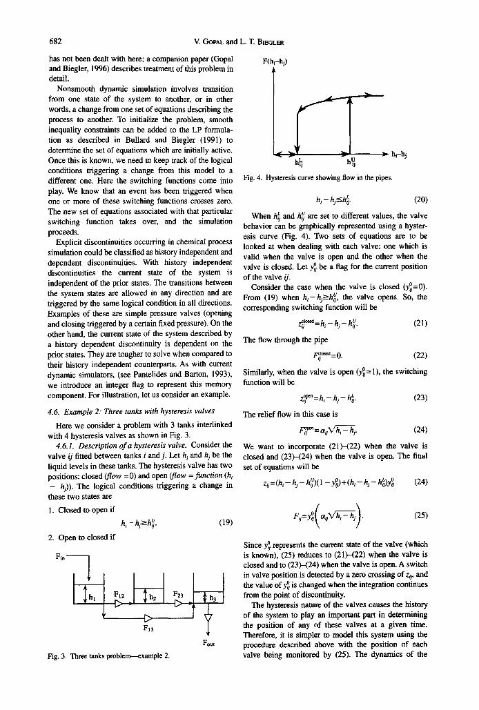
F(hi-hj)
hi-hj h~ h,~
Fig. 4. Hysteresis curve showing flow in the pipes.
hi- %---hb. (20) When h~ and h~. are set to different values, the valve
behavior can be graphically represented using a hyster- esis curve (Fig. 4). Two sets of equations are to be looked at when dealing with each valve: one which is valid when the valve is open and the other when the valve is closed. Let yO be a flag for the current position of the valve ij.
Consider the case when the valve is closed (y°=0). - - > U From (19) when h i h j_h o, the valve opens. So, the
corresponding switching function will be
~ l ° ~ a = h i - h j - h ~. (21)
The flow through the pipe
~'o~=0. (22)
Similarly, when the valve is open (yO= 1), the switching function will be
z~ ~" = h i - hj - h~. (23)
The relief flow in this case is
,b-~j" = ~ 0 ~ . (24)
We want to incorporate (21)-(22) when the valve is closed and (23)-(24) when the valve is open. The final set of equations will be
u - Yo) + (hi - hj - hij)y 0 (24) z o = ( h i _ h j _ h o ) ( 1 o L o
(25)
Since y~ represents the current state of the valve (which is known), (25) reduces to (21)-(22) when the valve is closed and to (23)-(24) when the valve is open. A switch in valve position is detected by a zero crossing of zij, and the value ofy ° is changed when the integration continues from the point of discontinuity.
The hysteresis nature of the valves causes the history of the system to play an important part in determining the position of any of these valves at a given time. Therefore, it is simpler to model this system using the procedure described above with the position of each valve being monitored by (25). The dynamics of the

Nonsmooth dynamic simulation
system of tanks and valves in Fig. 3 can be modeled using (26).
dhl At--~ =Fj,,- Fn- FI3
dh2 A2 ~ - = F n - F23
A dh3 3 ~ - = Ft3 - F23 - Fo,,
Fi)=y°.(otijh~i-h~) ij= 12,13,23,34
150 hi
............. h 2
lOO- - . . . . . . h3
m
50 - ...-,,.,. ::"
i | !
0 I 2
Time
Fig. 5. Height of liquid in the tanks.
683
z:(, , , h )y° (] = 12,13,23,34
(h4=0). (26)
The variables h are the liquid levels in the tanks, F the flowrates in the pipes and a the valve constants. This
system was simulated using the LP based algorithm. The values for the valve constants and the breakpoints are
given in Table 2. The initial conditions correspond to all tanks empty and all valves closed. It should be noted that at this initial point, care must be taken in the initializa- tion, as the valve positions are related to the initial liquid levels and cannot be specified arbitrarily. The constants were chosen to demonstrate the opening and closing of all the valves within a short time. Fig. 5 shows the levels of liquid in the three tanks. The driving force, the difference in liquids levels in the tanks is plotted in Fig. 6. The flowrate in the pipes is shown in Fig. 7.
5. I m p f i c i t d i s c o n t i n u i t i e s
In this section we consider a class of implicitly discontinuous problems encountered often in chemical process simulation: calculation of phase equilibrium. Consider a simple isothermal flash (Fig. 8) to highlight some of the basic issues which are relevant in this problem. A feed stream of composition z enters the flash column at a specified temperature and pressure. The products are a vapor phase stream of composition y and a fractional flowrate V and/or a liquid phase stream of
Table 2. Parameters for the three tanks problem
i/ h~ h~ %
12 30 75 12 13 60 100 12 23 30 50 15
3 out 40 50 10
composition x. Different sets of equations are valid depending on the number of phases present at equilib- rium. For example, the equilibrium equations are generally not valid in either of the single phase regions. The combined set of equations is an implicitly non- smooth problem with well defined smooth regions. Thus, one of the basic problems associated with phase equilibrium calculations, especially in an equation oriented simulation environment, is that the number of phases is not known a priori.
Among the different approaches suggested to tackle this problem, the classical sequential modular approach is the most familiar one (Boston and Britt, 1978; Nelson, 1987). In general, these methods calculate the bubble and dew points (in the case of two phase calculations) and then determine the number of phases at equilibrium.
hl-h 2
.............. hl-h3
. . . . . . h2._h3
............ h 3 I00.
4 ' : ..,: .C ::.
75 .............. , ........ ::
50-
/ I',, , / / ,,.. ...........
I! i ~ I o ! 2
Time
Fig. 6. The difference in levels of liquid in the tanks.
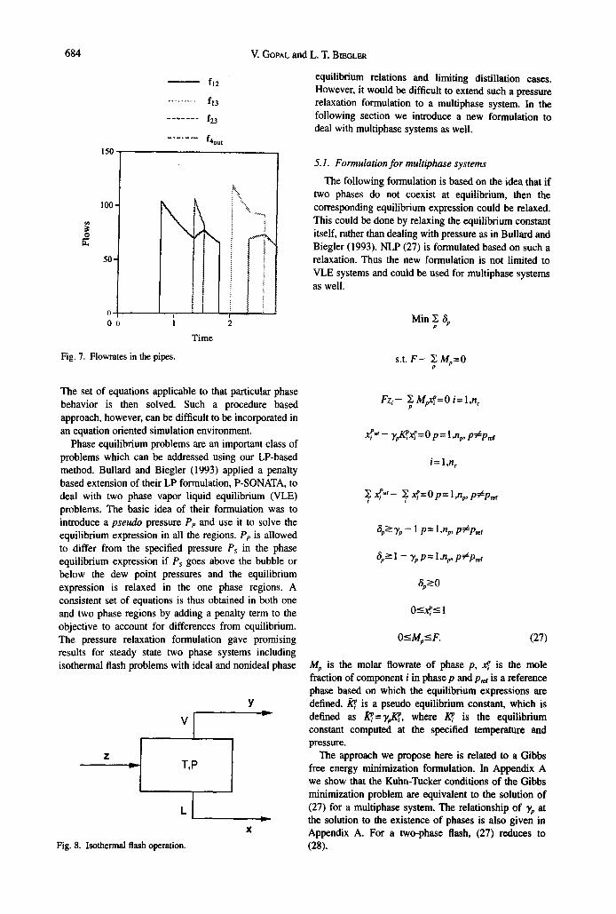
684 V. GOPAL and L. T. BIEGLER
150-
. . . . , , . . , . . . .
f12
f13
f23
f4out
100-
O
50.
0 . . . . ;
0 1 2
Fig. 7. Flowrates in the pipes.
Time
equilibrium relations and limiting distillation cases. However, it would be difficult to extend such a pressure relaxation formulation to a multiphase system. In the following section we introduce a new formulation to deal with multiphase systems as well.
5.1. Formulation for multiphase systems
The following formulation is based on the idea that if two phases do not coexist at equilibrium, then the corresponding equilibrium expression could be relaxed. This could be done by relaxing the equilibrium constant itself, rather than dealing with pressure as in Bullard and Biegler (1993). NLP (27) is formulated based on such a relaxation. Thus the new formulation is not limited to VLE systems and could be used for multiphase systems as well.
Min pE 6p
s.t. F - Y. Mp=O
The set of equations applicable to that particular phase behavior is then solved. Such a procedure based approach, however, can be difficult to be incorporated in an equation oriented simulation environment.
Phase equilibrium problems are an important class of problems which can be addressed using our LP-based method. Bullard and Biegler (1993) applied a penalty based extension of their LP formulation, P-SONATA, to deal with two phase vapor liquid equilibrium (VLE) problems. The basic idea of their formulation was to introduce a pseudo pressure Pp and use it to solve the equilibrium expression in all the regions. Pe is allowed to differ from the specified pressure Ps in the phase equilibrium expression if Ps goes above the bubble or below the dew point pressures and the equilibrium expression is relaxed in the one phase regions. A consistent set of equations is thus obtained in both one and two phase regions by adding a penalty term to the objective to account for differences from equilibrium. The pressure relaxation formulation gave promising results for steady state two phase systems including isothermal flash problems with ideal and nonideal phase
V
z _ I T,P
,I Fig. 8. Isothermal flash operation.
Y
Fzi- ~ Mzv~, =O i= l,nc
x~'/'~ -- yt,K~ =0 p= l,n,, p~p~f
i -~. l , n c
~ g " - ~=Op=l.n, .p¢p~ r
8,>yp - 1 p= 1,n,, p¢p,~f
6,-- > 1 - 7, P= l,n,, P~Pref
a,~0
0_<~_< 1
O<Mp<--F. (27)
Alp is the molar flowrate of phase p, ~ is the mole fraction of component i in phase p and Pref is a reference phase based on which the equilibrium expressions are defined. ~ is a pseudo equilibrium constant, which is defined as ~=yflC~, where ~ is the equilibrium constant computed at the specified temperature and pressure.
The approach we propose here is related to a Gibbs free energy minimization formulation. In Appendix A we show that the Kuhn-Tucker conditions of the Gibbs minimization problem are equivalent to the solution of (27) for a multiphase system. The relationship of yp at the solution to the existence of phases is also given in Appendix A, For a two-phase flash, (27) reduces to (28).

Nonsmooth dynamic simulation 685
Mira5 Min8
s.t. F - L - V=0
F z i - Lxi - Vyi=O i= 1,n
Yi - yKi(P,T,x)xl =0 i= l,n
~i yi - ~i xi=O
~$>-- y - 1
8>__1 - y
6>_0
O<--xi,Yi<--I
O<--L,V<--F. (28)
In the two phase region, y = 1 and the equilibrium expression is satisfied. In the single phase regions, y differs from 1 and the equilibrium expression is relaxed. In Appendix A we show that y > 1 in the single phase liquid region and y <1 in the single phase vapor region.
Recently Swaney and Kendlbacher (1994) expressed the complementarity condition equivalently as
~ ~ - 1 + ~'= 0 (29)
where the slacks ~ and the phase amounts M v (e.g., V or L p) are complementary:
AP->0 gP->0 MP~=0. (30)
Such a formulation could also be solved reliably using iterated LE In fact, the optimality conditions of (27) could be simplified to an equation based formulation similar to the one in Swaney and Kendlbacher (1994). In Appendix B we present the equation based simplified formulation derived from the optimality conditions of the two phase problem (28).
5.2. Example 3. Dynamic simulation of a two-phase flash tank covering three regimes o f operation
In this example we consider an n-butane, n-pentane, n-hexane system where the ideal flash unit is modeled using the Antoine equation. A constant feed of mole fractions 0.3, 0.3 and 0.4 for the respective components is supplied to the unit. The flash is carried out at a pressure of 7600 mm Hg. The temperature is varied linearly from Ti =385 K to T I =420 K from time t0=0 to tf = 10. It should be noted that the dew and bubble points of the feed lie in this range. The motivation behind choosing this example problem is to see whether the algorithm could capture the transition from a single phase region to a two phase region and vice versa as the temperature was varied.
dH s.t. ~ = f - Vy-Lx
m at v - L
H=Mtx
L= otVM,,
y = yK(T)x
EiYi- ~ixi=O
T=T(t)
- 6 < - y - 1~6
8>0
O<---xi,Yi < -- 1. (31 )
The flash unit was modeled as in (31) where L is the liquid flowrate, V is the vapor flowrate, H is the component molar holdup, x and y are the component mole fractions in the liquid and vapor phases and M I is the total liquid holdup. All variables in (31) are functions of time. Vapor holdup is neglected in this formulation. The holdups were discretized using implicit Euler and the corresponding set of equations was solved using iterated LP at time steps of 0.1. Fig. 9 shows the liquid and vapor stream flowrates with time.
The plot indicates that the algorithm handled the transition from the single phase liquid region to the two phase region and then to the single phase vapor region well. The average number of iterations for solving the problem per time step was 4.1. In the single phase regions, solution of the discretized equations on an average took 3 iterations. The problem, when discretized with smaller steps and when solved using a second order method, trapezoidal rule, gave similar results.
1 2 5
1oo-
75
50
25 ̧
L
2 4 6 8 io
t
Fig. 9. Liquid and vapor flowrates in example 3.

686 V. Gor,~ and L. T. BIF~LER
5.3. Example 4. Dynamic simulation of a nonideal three phase flash
This example examines a benzene--isopropanol-water system considered in steady state by Pham and Doherty (1990). For different temperature-pressure conditions this system could exist as a LLV (liquid-liquid-vapor) or LL (liquid-liquid) or LV (liquid-vapor) or just as a single phase liquid or single phase vapor. To accom- modate these possibilities, we posed the formulation (32) for the dynamic simulation of this system.
Minff+ff I
dH s.t. ~ - = f - Vy - LIx a - L#x #
d : (~ , + M~') = ~/f, - V - L I - L" dt
H = ~? + ~'x"
t_,'=dV'-~, t/'--d'V'-~, y = ,~Klx I
y= ~/qKUx n
~ / y , - ~ .~=0
~y,- ~ ~,'=0
T=T(t)
- ~ < - ~ / - 1<-~
- ~1<_ ~ / I - 1 < _ ~ ,
~,~"->0
0 - < ~ , y , - - < 1 (32)
As in example 3, a constant feed of mole fractions 0.5, 0.08 and 0.42 of benzene, isopropanol and water respectively was fed into the flash tank. At constant pressure of 1 atm, the temperature is decreased linearly from 70°C to 68°C. The initial conditions correspond to steady state values at 70°C.
The activity coefficients for this system were calcu- lated using the regular solution model. Fig. 10 plots the flowrates of the two liquid and the vapor streams with time. Liquid phases 1 and 2 correspond to the water rich and benzene rich phases respectively. As shown in the figure, initial conditions correspond to a liquid-vapor system. A second liquid phase appears later on and the system enters the three phase L ~ - L II - V region. Upon further decrease of temperature, the vapor phase van- ishes altogether, resulting in a two phase liquid region. The algorithm was thus successful in simulating the three phase LLV and the two phase LV and LL regions with a single formulation. An average of 3.4 iterations was required to solve the discretized equations at each time step.
Both examples show that the penalty based iterative LP strategy could be a strong tool for solving dynamic problems involving phase transitions, without having to compute the dew and bubble points and then determin- ing the number of phases at any time. The transitions between phase combinations were handled efficiently by a single consistent formulation. Recently, several studies (McDonald and Floudas, 1994; Swaney and Kendl- bacher, 1995; Stadtherr et al., 1995; Sun and Seider, 1995) describe global algorithms for solving phase equilibrium problems of this type and for assessing the stability by using the tangent plane criterion. Beyond initialization and at a limited number of points, however, applying a global optimization algorithm to dynamic phase equilibrium problems could be expensive and often unnecessary. Instead, the equilibrium solution at a particular time step gives good starting points for the problem at the next time step, and therefore tracks the
0.8
0.6
0.4
0.2
~ o o o o o o ~ z ~ LI
...... o ....... L2
~. o v
s I
- o. ~ O . "
~ ' , , ~ < ~
0 0.5 I 1.5 2
t
Fig. 10. Flowrates of the two liquid and vapor streams in example 4.

Nonsmooth dynamic simulation
optimum locally. A formulation such as the one presented in this paper has its relevance in this context.
6. Conclusions
A previously developed LP-based method has been extended to a variety of dynamic simulation problems. The method has been refined with the addition of a new descent strategy which combines line search with a trust region approach. The LP based method has been demonstrated to be an effective way for the imposition of bounds on variables in dynamic simulation problems. An improved method for the treatment of discontinuities occurring in nonsmooth dynamic simulation problems has been developed. The method ensures that any event which has occurred within the time interval in considera- tion is detected, and if more than one event occurs, the detected one is indeed the earliest one. In the case of nonexistence of solution across a discontinuity, a penalty term introduced in our approach makes it less likely to fail when compared to the presently used discontinuity locking methods. A specific class of process simulation problems, phase equilibrium calculations, has been looked at as a special case. A new formulation for solving multiphase equilibrium problems has been presented. A penalty term introduced in the objective takes care of the appearance and disappearance of phases. Example problems have been solved to demon- strate the feasibility of the approach.
With the results from small problems being encourag- ing, future work will focus on solving large scale problems. An LP interface to a sparse DAE solver like SDASSL is expected to be an efficient way of dealing with large nonsmooth dynamic simulation problems. The LP will provide an efficient way for dealing with variable bounds and conditionals, whereas the DAE solver will automatically generate the polynomial func- tions for the detection of discontinuities.
Acknowledgements
Funding for this work was provided by the Engineering Design Research centre at CMU. The authors are also grateful for the helpful suggestions of Profs Marquardt and Barton.
References
Armijo, L. (1966) Minimization of functions having Lipschitz continuous first partial derivatives. Pacific J. Math. 16, 1
Barrodale, I. and Roberts, ED.K. (1978) An efficient algorithm for discrete L1 linear approximations with linear constraints. SlAM J. Numer. Anal 15, 3
Barton, P. I. (1992) Ph.D. Dissertation, Imperial College of Science, Technology and Medicine, London, UK.
Biegler, L.T., Damiano, J.J. and Blau, G.E. (1986) Nonlinear parameter estimation: A case study comparison. AIChE J. 32, 1 29
Blau, G. E., Kirby, L. and Marks, M. (1981) An
687
industrial kinetics problem for testing nonlinear parameter estimation algorithms, Process Math Modeling Department, The Dow Chemical Com- pany.
Brenan, K. E., Campbell, S. L. and Petzold, L. R. (1996) Numerical Solution of Initial-Value Problems in Differential-Algebraic Equations, SIAM, Philadel- phia.
Boston, J.E and Britt, H.L. (1978) A radically different formulation and solution of the single-stage flash problem. Computers Chem. Engng. 2, 109
Bullard, L. G. (1991) Ph.D. Dissertation, Carnegie Mellon University, Pittsburgh, PA).
Bullard, L.G. and Biegler, L.T. (1991) Iterative linear programming strategies for constrained simulation. Computers Chem. Engng. 15, 239
Bullard, L.G. and Biegler, L.T. (1993) Iterated linear programming strategies for nonsmooth simulation: a penalty based method for vapor-liquid equilib- rium applications. Computers Chem. Engng. 17, 95
Chamberlein, R.M., Powell, M.J.D., Lemerchal, C. and Pedersen, H.C. (1982) The watchdog method for forcing convergence in algorithms for constrained optimization. Math. Prog. 16, 1
Dennis, J. E. and Schnabel, R. B. (1983) Numerical Methods for Unconstrained Optimization and Non- linear Equations. Prentice-Hall, Inc., Englewood Cliffs, NJ.
Duff, I.S., Nocedal, J. and Reid, J.K. (1987) The use of linear programming for the solution of sparse sets of nonlinear equations. SIAM J. Sci. Statist. Corn- put. 8, 99
Fletcher, R. (1987) Practical Methods of Optimization. Wiley, New York.
Gopal, V. and Biegler, L. T. (1996) An optimization approach to consistent initialization and reinitializa- tion after discontinuities of differential algebraic equations, Fifth SIAM Conference on Optimization, Victoria, Canada.
Gill, E E., Murray, W., Saunders, M. A. and Wright, M. H. (1983) User's Guide for SOL/QPSOL: A Fortran Package for Quadratic Programming, Tech- nical Report SOL 83-7, Department of Operations Research, Stanford University, Stanford, CA.
Joglekar, G.S. and Reklaitis, G.V. (1984) A simulator for batch and semi-continuous processes. Computers Chem. Engng. g, 315
Marquardt, W. (1991) Dynamic process simulation-- recent progress and future challenges. In: Chemical Process Control (Edited by Y. Arkun and W. H. Ray), CACHE-AIChE Publications, 131.
McDonald, C.M. and Floudas, C.A. (1994) Decomposi- tion based and branch and bound global optimiza- tion approaches for the phase equilibrium problem. Journal of Global Optimization 5, 205
Naess, U, Mjaavatten, A. and Li, J. (1992) Using dynamic process simulation from conception to normal operation of process plants. Computers Chem. Engng. 16, Sll9
Nelson, EA. (1987) Rapid phase determination in multiple-phase flash calculations. Computers Chem. Engng. 11, 6
Pantelides, C.C. (1988) SpeedUp--Recent advances in process simulation. Computers Chem. Engng. 12, 745

688 V. GOPAL and L. T. BIEGLER
Pantelides, C.C. and Barton, EI. (1993) Equation- oriented dynamic simulation: current status and future perspectives. Computers Chem. Engng. 17, $263
Park, T. and Barton, E I. (1993) A new algorithm for the accurate and efficient location of state events, Special Topical Conference on Industrial Chemical Technology, AIChE Annual Meeting, St. Louis, MO.
Perkins, J.D. (1986) Survey of existing systems for the dynamic simulation of industrial processes. Model- ing, Identification and Control 7, 71
Pham, H.H. and Doherty, M.F. (1990) Design and Define synthesis of heterogeneous azeotropic distilla- t i o n s - I , Heterogeneous phase diagrams. Chem. Engng. Sci. 45, 7
Smith, G.J. and Morton, W. (1988) Dynamic simulation using an equation-oriented flowsheeting package. Computers Chem. Engng. 12, 469
Stadtherr, M. A., Schnepper, C. A. and Brennecke, J. F. (1995) Robust phase stability analysis using inter- val methods. In: Fourth International Conference on Foundations of Computer-Aided Process Design (Edited by L. T. Biegler and M. E Doherty), 356 pp. CACHE-AIChE Publications.
Sun, A.C. and Seider, W.D. (1995) Homotopy-continua- tion method for stability analysis in the global minimization of the Gibbs free energy. Fluid Phase Equilibria 103, 213
Swaney, R. E. and Kendlbacher, T. (1994) Robust solution of phase equilibrium calculations, AIChE Annual Meeting, San Francisco, CA.
Zhang, J., Kim, N. and Lasdon, L. (1985) An improved successive linear programming algorithm. Mgmt Sci. 31, 10
Appendix A: Mull iphase formulation
We show that the solution of the formulation (16) for multiphase systems would satisfy the Kuhn-Tucker conditions of a Gibbs free energy minimization formulation.
For an n component, p phase mixture, the Gibbs minimiza- tion formulation would be
s.t. 2 ~=n r i= 1,n~ p
E ~>--0 p= 1,rip (33)
where ~ denotes the moles of component i in phase p. Simplifying (33),
Min G = ~ n~AG~+ ~ ~ ~RTInf~
S.t. ~ ~=n~ i= l,n c
~ ~ 0 p = 1,np. (34)
The Kuhn-Tucker conditions of the problem can be simplified tO
• ~ Oln£ RTInfl~+RT2 e 2j , ~ + a : g = 0 i=l,n~ pfl,np (35)
g ,2 ~=0 p=lmp (36)
where a~ and/3p are the multipliers for the equalities and the inequalities respectively.From the Gibbs-Duhem theorem,
. OlnZ/ ,,
~p=RTInF r (37)
(35) reduces to RTIn ~ =% a constant for component i in all r, phases or
~--~" = ~---~" Yp,~,p.. (38) r,. r,.
If E ~=/W'=0, where Mp is the molar flowrate of phase p, (36)
//p 0 and hence (37) ~ Fp l.On the other hand if Mp 0, (36) ,Sp =0 and hence (37) ~ F e = 1. ie.
~ = l~phase p exists
Fe> l~phase p does not exist. (39)
Define a reference phase p~. (38) can be written as
-~ = -~p p = l,nl,,p~p,a i= l,n~ (40)
But
(40) simplifies to
:,=p~ (41)
¢.__(r,.\/~, \ --~p )~)~ p=l,ne,p.p, i=l,n c (42)
~= 7~gT~ (43)
where
yp= ~ ,a constant (44)
and
dr*. ~ = ~ , ~ the equilibrium constant for phases p and P,a. (45)
(43) could be written as
where ~ is a pseudo equilibrium constant. Note that ~=K~ when both phases p and p~ coexist.For the flash operation, ~--Mr~, so we can express the flash problem using the penalty formulation as in (27), which will reduce to (28) for a two phase system (with the vapor phase as the reference phase).

Nonsmoo t h dynamic s imulat ion
The following shows the correlation of the values of % to the existence of phases:
• 3'p < 1 ~ Fp > Fp,.f ~ F, > 1 ~ phase p does not exist • 3'~ >3'pn~ Fp,~ >Fpm~Fp , >1 ~ p h a s e p . does not exist • Any % >1 ~ Fmf > Fp ~ Fmf >1 ~ phase p~f does not
exist.
For a two phase system this becomes:
• y = 1 ~ both liquid and vapor phases exist • 3' > 1 ~ vapor phase does not exist • 3' < 1 ~ liquid phase does not exist.
A p p e n d i x B: E q u a t i o n b a s e d f o r m u l a t i o n f o r (28)
The optimality conditions of the two phase flash (28) can be simplified to the form (47)-(57).
F - L - V=0 (47)
Fz i - Lx i - Vy~=O i= 1,n (48)
y~- yK~(P,T~c)x,=O i= 1,n (49)
Yl - ~ x,=O (50)
- 6+ 3 ' - 1 +s+=0 (51)
- 6 - 3'+ 1 +s_=O (52)
s+L=0 (53)
s_ V=0 (54)
8,s+,s_->O (55)
O<-xi,yi < - 1 (56)
O<-L,V<-F. (57)
The key here is recognizing that the multipliers for the slacks s . and s_ correspond to the phase amounts L and V respectively. (53) and (54) are strict complementarity conditions. Below we
689
will show that the above formulation is equivalent to the conditions on Y derived from the Gibbs free energy formula- tion, presented at the end of <appr id= "A". Consider the three c a s e s ;
• y > l
From (51)-(52),
6 - s+=s_ - 6 = y - 1 >0. (58)
It can be shown that
6= 3 ' - 1. (59)
(If 6>3' - 1 , s+>0 ~ L =0 from (53). Also s_>6 3 ' - 1 >0 = V =0. L,V =0 will not satisfy (47)--(48) for a nonzero feed flowrate) From (58) and (59), we have
s+=0, s_ =2(3 ' - 1). (60)
From (53) and (54)
L>0, V=0. (61)
Hence, this corresponds to a single phase liquid case.
• 3'<1
As above, it can be shown that
6=1 - 3'
s _ = 0 (62)
s .=2( l - 3'). (63)
From (53) and (54)
L=0, V>0. (64)
This corresponds to a single phase vapor region.
• y = l .
In this case
6=s÷=s÷=O. (65)
From the strict complementarity conditions, L,V O, corre- sponding to the two phase region.
CA~ 21-7-8