Embed Size (px)
Citation preview
arX
iv:1
412.
1922
v1 [
stat
.AP]
5 D
ec 2
014
The Annals of Applied Statistics
2014, Vol. 8, No. 3, 1825–1852DOI: 10.1214/14-AOAS759c© Institute of Mathematical Statistics, 2014
NONSTATIONARY ETAS MODELS FORNONSTANDARD EARTHQUAKES
By Takao Kumazawa1,∗ and Yosihiko Ogata1,2,∗,†
The Institute of Statistical Mathematics∗ and University of Tokyo†
The conditional intensity function of a point process is a usefultool for generating probability forecasts of earthquakes. The epidemic-type aftershock sequence (ETAS) model is defined by a conditionalintensity function, and the corresponding point process is equivalentto a branching process, assuming that an earthquake generates acluster of offspring earthquakes (triggered earthquakes or so-calledaftershocks). Further, the size of the first-generation cluster dependson the magnitude of the triggering (parent) earthquake. The ETASmodel provides a good fit to standard earthquake occurrences. How-ever, there are nonstandard earthquake series that appear under tran-sient stress changes caused by aseismic forces such as volcanic magmaor fluid intrusions. These events trigger transient nonstandard earth-quake swarms, and they are poorly fitted by the stationary ETASmodel. In this study, we examine nonstationary extensions of theETAS model that cover nonstandard cases. These models allow theparameters to be time-dependent and can be estimated by the empir-ical Bayes method. The best model is selected among the competingmodels to provide the inversion solutions of nonstationary changes.To address issues of the uniqueness and robustness of the inversionprocedure, this method is demonstrated on an inland swarm activityinduced by the 2011 Tohoku-Oki, Japan earthquake of magnitude 9.0.
1. Introduction. The epidemic-type aftershock sequence (ETAS) model[Ogata (1985, 1986, 1988, 1989)] is one of the earliest point-process modelscreated for clustered events. It is defined in terms of a conditional inten-sity [Hawkes (1971), Hawkes and Adamopoulos (1973), Ogata (1978, 1981)],
Received October 2013; revised April 2014.1Supported by JSPS KAKENHI Grant Numbers 23240039 and 26240004, supported
by a postdoctoral fellowship from the Institute of Statistical Mathematics.2Supported by the Aihara Innovative Mathematical Modelling Project, the “Funding
Program for World-Leading Innovative R&D on Science and Technology (FIRST Pro-gram),” initiated by the Council for Science and Technology Policy.
Key words and phrases. Akaike Bayesian Information Criterion, change point, two-stage ETAS model, time-dependent parameters, induced seismic activity.
This is an electronic reprint of the original article published by theInstitute of Mathematical Statistics in The Annals of Applied Statistics,2014, Vol. 8, No. 3, 1825–1852. This reprint differs from the original in paginationand typographic detail.
1
2 T. KUMAZAWA AND Y. OGATA
is equivalent to epidemic branching processes [Kendall (1949), Hawkes andOakes (1974)], and allows each earthquake to generate (or trigger) offspringearthquakes. Besides being used in seismology, the ETAS model has been ap-plied to various fields in the social and natural sciences [e.g., Balderama et al.(2012), Chavez-Demoulina and Mcgillb (2012), Hassan Zadeh and Sharda(2012), Herrera and Schipp (2009), Mohler et al. (2011), Peng, Schoenbergand Woods (2005), Schoenberg, Peng and Woods (2003)].
Similar magnitude-dependent point-process models have been applied toseismological studies [Vere-Jones and Davies (1966), Lomnitz (1974), Kaganand Knopoff (1987)] and statistical studies [Vere-Jones (1970)]. The ETASmodel is stationary if the immigration rate (background seismicity rate)of an earthquake remains constant and the branching ratio is subcritical[Hawkes (1971), Hawkes and Oakes (1974), Zhuang and Ogata (2006)].
The history-dependent form of the ETAS model on occurrence times andsizes (magnitudes) lends itself to the accumulated empirical studies by Utsu(1961, 1962, 1969, 1970, 1971, 1972) and Utsu and Seki (1955), and itsestablishing history is detailed by Utsu, Ogata and Matsu’ura (1995). ETASmodel parameters can be estimated from earthquake occurrence data bymaximizing the log-likelihood function to provide estimates for predictingseismic activity (i.e., number of earthquakes per unit time). The model hasbeen frequently used and cited in seismological studies, especially to comparethe features of simulated seismicity with those of real seismicity data. Themodel is also recommended for use in short-term predictions [Jordan, Chenand Gasparini (2012)] in the report of the International Commission onEarthquake Forecasting for Civil Protection. It is planned to be adopted foroperational forecasts of earthquakes in California (The Uniform CaliforniaEarthquake Rupture Forecast, Version 3, URL: http://www.wgcep.org/sites/wgcep.org/files/UCERF3_Project_Plan_v55.pdf).
The ETAS model has also been used to detect anomalies such as quies-cence in seismicity. Methods and applications are detailed in Ogata (1988,1989, 1992, 1999, 2005, 2006a, 2007, 2010, 2011a, 2012), Ogata, Jones andToda (2003), Kumazawa, Ogata and Toda (2010), and Bansal and Ogata(2013). A change-point analysis examines a simple hypothesis that specificparameters change after a certain time. The misfit of occurrence rate pre-diction after a change point is then preliminarily shown by the deviation ofthe empirical cumulative counts of the earthquake occurrences from the pre-dicted cumulative function. The predicted function is the extrapolation ofthe model fitted before the change point. A downward and upward deviationcorresponds to relative quiescence and activation, respectively.
This study considers a number of nonstationary extensions of the ETASmodel to examine more detailed nonstandard transient features of earth-quake series. The extended models take various forms for comparison withthe reference ETAS model, which represents the preceding normal activity
NONSTATIONARY ETAS MODELS 3
in a given focal region. Because changing stresses in the crust are not directlyobservable, it is necessary to infer relevant quantitative characteristics fromseismic activity data. For example, Hainzl and Ogata (2005) and Lombardi,Cocco and Marzocchi (2010) estimated time-dependent background rates(immigration rates) in a moving time window by removing the triggeringeffect in the ETAS model.
In Section 2, time-dependent parameters for both background rates andproductive rates are simultaneously estimated. There, the penalized log-likelihood is considered for the trade-off between a better fit of the non-stationary models and the roughness penalties against overfitting. Then,not only is an optimal strength adjusted for each penalty but also a betterpenalty function form is selected using the Akaike Bayesian Information Cri-terion (ABIC ) [Akaike (1980)]. These parameter constraints together withthe existence of a change point are further examined to determine if theyimprove the model fit. One benefit of this model is that it allows varying pa-rameters to have sharp changes or discontinuous jumps at the change pointwhile sustaining the smoothness constraints in the rest of the period.
In Section 3, the methods are demonstrated by applying the model to aswarm activity. The target activity started after the March 11, 2011 Tohoku-Oki earthquake of magnitude (M) 9.0, induced at a distance from the M9.0rupture source. Section 4 concludes and discusses the models and methods.The reproducibility of the inversion results is demonstrated in the Appendixby synthesizing the data and re-estimating it using the same procedure.
2. Methods.
2.1. The ETAS model. A conditional intensity function characterizes apoint (or counting) process N(t) [Daley and Vere-Jones (2003)]. The condi-tional intensity λ(t|Ht) is defined as follows:
Pr{N(t, t+ dt) = 1|Ht}= λ(t|Ht)dt+ o(dt),(1)
where Ht represents the history of occurrence times of marked events upto time t. The conditional intensity function is useful for the probabilityforecasting of earthquakes, which is obtained by integrating over a timeinterval.
The ETAS model, developed by Ogata (1985, 1986, 1988, 1989), is aspecial case of the marked Hawkes-type self-exciting process, and has thefollowing specific expression for conditional intensity:
λθ(t|Ht) = µ+∑
{i : S<ti<t}
K0eα(Mi−Mz)
(t− ti + c)p,(2)
where S is the starting time of earthquake observation and Mz representsthe smallest magnitude (threshold magnitude) of earthquakes to be treated
4 T. KUMAZAWA AND Y. OGATA
in the data set. Mi and ti represent the magnitude and the occurrencetime of the ith earthquake, respectively, and Ht represents the occurrenceseries of the set (ti, Mi) before time t. The parameter set θ thus consistsof five elements (µ, K0, c,α, p). In fact, the second term of equation (2) is aweighted superposition of the Omori–Utsu empirical function [Utsu (1961)]for aftershock decay rates,
λθ(t) =K
(t+ c)p,(3)
where t is the elapsed time since the main shock. It is important to notethat, while the concept of a main shock and its aftershocks is intuitively clas-sified by seismologists sometime after the largest earthquake occurs, there isno clear discrimination between them in equation (2). That is, each earth-quake can trigger aftershocks, and the expected cluster size depends on themagnitude of the triggering earthquake with the parameter α.
The parameter K0 (earthquakes/day) is sometimes called the “aftershockproductivity.” As the name explains, the parameter controls the overall trig-gering intensity. The factor c (day) is a scaling time to establish the power-law decay rate and allows a finite number of aftershocks at the origin timeof a triggering earthquake (a main shock). In practice, the fitted values forc are more likely to be caused by the under-reporting of small earthquakeshidden in the overlapping wave trains of large earthquakes [Utsu, Ogata andMatsu’ura (1995)]. The exponent p is the power-law decay rate of the earth-quake rate in equation (3). The magnitude sensitivity parameter α (magni-tude −1) accounts for the efficiency of an earthquake of a given magnitudein generating aftershocks. A small α value allows a small earthquake to trig-ger a larger earthquake more often. Finally, the background (spontaneous)seismicity rate µ represents sustaining external effects and superposed oc-currence rates of long-range decays from unobserved past large earthquakes.It also accounts for the triggering effects by external earthquakes.
The FORTRAN program package associated with manuals regardingETAS analysis is available to calculate the maximum likelihood estimates(MLEs) of θ and to visualize model performances [Ogata (2006b)]. See alsohttp://www.ism.ac.jp/~ogata/Ssg/ssg_softwaresE.html.
2.2. Theoretical cumulative intensity function and time transformation.
Suppose that the parameter values θ = (µ,K, c,α, p) of the ETAS, equation(2), are given. The integral of the conditional intensity function,
Λθ(t|Ht) =
∫ t
Sλθ(u|Hu)du,(4)
provides the expected cumulative number of earthquakes in the time inter-val [0, t]. The time transformation from t to τ is based on the cumulative
NONSTATIONARY ETAS MODELS 5
intensity,
τ =Λ(t|Ht),(5)
which transforms the original earthquake occurrence time (t1, t2, . . . , tN ) intothe sequence (τ1, τ2, . . . , τN ) in the time interval [0,Λ(T )]. If the model rep-resents a good approximation of the real seismicity, it is expected that theintegrated function [equation (4)] and the empirical cumulative counts N(t)of the observed earthquakes are similar. This implies that the transformedsequence appears to be a stationary Poisson process (uniformly distributedoccurrence times) if the model is sufficiently correct, and appears to be het-erogeneous otherwise.
2.3. Two-stage ETAS model and the change-point problem. In change-point analysis, the whole period is divided into two disjointed periods tofit the ETAS models separately, and is therefore called a two-stage ETASmodel. This is one of the easiest ways to treat nonstationary data, and is bestapplied to cases in which parameters are suspected to change at a specifictime. Such a change point is observed when a notably large earthquake orslow slip event (regardless of observed or unobserved) occurs in or near afocal region. Many preceding studies [e.g., Ogata, Jones and Toda (2003),Ogata (2005, 2006a, 2007, 2010), Kumazawa, Ogata and Toda (2010)] haveadopted this method to their case studies, and details can be found therein.
The question of whether the seismicity changes at some time T0 in a givenperiod [S,T ] is reduced to a problem of model selection. In this analysis,the ETAS models are separately fitted to the divided periods [S,T0] and[T0, T ], and their total performance is compared to an ETAS model fittedover the whole period [S,T ] by the Akaike Information Criterion (AIC )[Akaike (1973, 1974, 1977)]. The AIC is described as follows:
AIC =−2max logL(θ) + 2k,(6)
where ln L(θ) represents the log-likelihood of the ETAS model,
logL(θ) =∑
{i : S<ti<T}
logλθ(ti|Hti)−∫ T
Slogλθ(t|Ht)dt,(7)
and k is the number of parameters to be estimated. The variables ti andHti are the same as those in equation (2). Under this criterion, the modelwith a smaller AIC value performs better. It is useful to keep in mindthat exp{−∆AIC/2} can be interpreted as the relative probability of howa model with a smaller AIC value is superior to others [e.g., Akaike (1980)].
Let AIC 0 be the AIC of the ETAS model estimated for the whole period[S,T ], AIC 1 be that of the first period [S,T0], and AIC 2 be that of the
6 T. KUMAZAWA AND Y. OGATA
second period [T0, T ], therefore,
AIC 0 =−2maxθ0
logL(θ0;S,T ) + 2k0,
AIC 1 =−2maxθ1
logL(θ1;S,T0) + 2k1,(8)
AIC 2 =−2maxθ2
logL(θ2;T0, T ) + 2k2.
Let AIC 12 represent the total AIC from the divided periods, such that
AIC 12 =AIC 1 +AIC 2 + 2q,(9)
with q being the degrees of freedom to search for the best change-pointcandidate T0. Next, AIC 12 is compared against AIC 0. If AIC 12 is smaller,the two-stage ETAS model with the change point T0 fits better than theETAS model applied to the whole interval. The quantity q monotonicallydepends on sample size (number of earthquakes in the whole period [S,T ])when searching for the maximum likelihood estimate of the change point[Ogata (1992, 1999), Kumazawa, Ogata and Toda (2010), Bansal and Ogata(2013)]. This penalty term q, as well as an increased number of estimatedparameters, imposes a hurdle for a change point to be significant, and itis usually rejected when the one-stage ETAS model fits sufficiently well. Ifthe change point T0 is predetermined from some information other thanthe data, then q = 0. This is often the case when a conspicuously largeearthquake occurs within swarm activity, and will be discussed below. Also,even in this case, the overfitting by the change point is avoided by the AIC 12
of a two-stage ETAS model, which has two times as many parameters of asingle stationary ETAS model throughout the whole period.
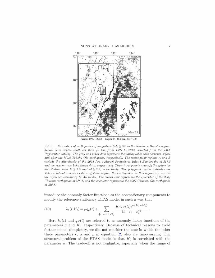
2.4. Anomaly factor functions for nonstationary ETAS models. Assumethat the ETAS model fits the data well for a period of ordinary seismicactivity. Then, the concern is whether this model shows a good fit to theseismicity in a forward extended period. If there are misfits, time-dependentcompensating factors are introduced to the parameters to be made time-dependent. These factors are termed “anomaly factor functions” and, thus,the transient changes in parameters are tracked. If earthquake activity isvery low in and near a target region preceding the transient activity, datafrom a wider region, such as the polygonal region in Figure 1, is used toobtain a reference stationary ETAS model (Figure 2). Such a model is sta-ble against small local anomalies, and is therefore a good reference model.The reference ETAS model, coupled with the corresponding anomaly factorfunctions, becomes the nonstationary ETAS model in this study.
Among the parameters of the ETAS model, the background rate µ andthe aftershock productivity K0 are sensitive to nonstationarity. We therefore
NONSTATIONARY ETAS MODELS 7
Fig. 1. Epicenters of earthquakes of magnitude (M)≥ 3.0 in the Northern Honshu region,Japan, with depths shallower than 40 km, from 1997 to 2012, selected from the JMAHypocenter catalog. The gray and black dots represent the earthquakes that occurred beforeand after the M9.0 Tohoku-Oki earthquake, respectively. The rectangular regions A and Binclude the aftershocks of the 2008 Iwate-Miyagi Prefectures Inland Earthquake of M7.2and the swarm near Lake Inawashiro, respectively. Their inset panels magnify the epicenterdistribution with M ≥ 2.0 and M ≥ 2.5, respectively. The polygonal region indicates theTohoku inland and its western offshore region; the earthquakes in this region are used inthe reference stationary ETAS model. The closed star represents the epicenter of the 2004Chuetsu earthquake of M6.8, and the open star represents the 2007 Chuetsu-Oki earthquakeof M6.8.
introduce the anomaly factor functions as the nonstationary components tomodify the reference stationary ETAS model in such a way that
λθ(t|Ht) = µqµ(t) +∑
{i : S<ti<t}
K0qK(ti)eα(Mi−Mz)
(t− ti + c)p.(10)
Here kµ(t) and qK(t) are referred to as anomaly factor functions of theparameters µ and K0, respectively. Because of technical reasons to avoidfurther model complexity, we did not consider the case in which the otherthree parameters c, α and p in equation (2) also are time-varying. Onestructural problem of the ETAS model is that K0 is correlated with theparameter α. The trade-off is not negligible, especially when the range of
8 T. KUMAZAWA AND Y. OGATA
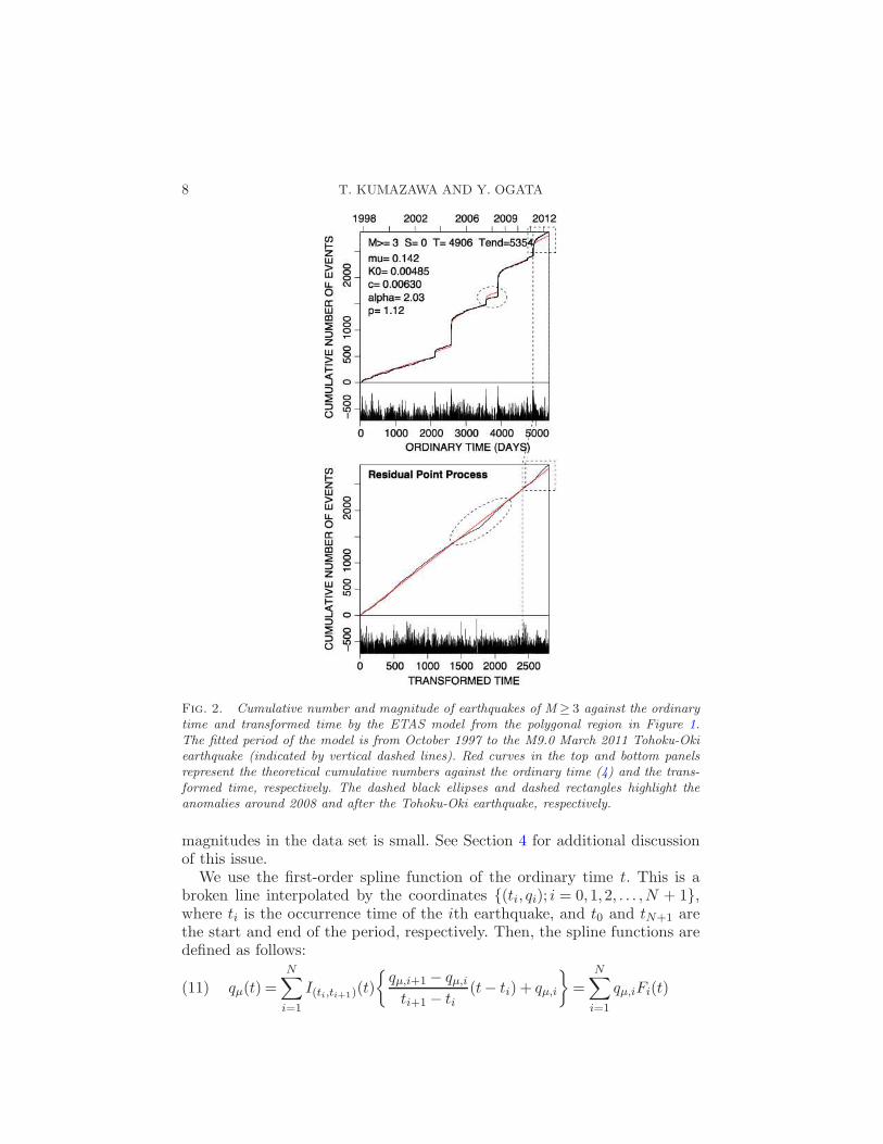
Fig. 2. Cumulative number and magnitude of earthquakes of M≥ 3 against the ordinarytime and transformed time by the ETAS model from the polygonal region in Figure 1.The fitted period of the model is from October 1997 to the M9.0 March 2011 Tohoku-Okiearthquake (indicated by vertical dashed lines). Red curves in the top and bottom panelsrepresent the theoretical cumulative numbers against the ordinary time (4) and the trans-formed time, respectively. The dashed black ellipses and dashed rectangles highlight theanomalies around 2008 and after the Tohoku-Oki earthquake, respectively.
magnitudes in the data set is small. See Section 4 for additional discussionof this issue.
We use the first-order spline function of the ordinary time t. This is abroken line interpolated by the coordinates {(ti, qi); i = 0,1,2, . . . ,N + 1},where ti is the occurrence time of the ith earthquake, and t0 and tN+1 arethe start and end of the period, respectively. Then, the spline functions aredefined as follows:
qµ(t) =N∑
i=1
I(ti,ti+1)(t)
{
qµ,i+1 − qµ,iti+1 − ti
(t− ti) + qµ,i
}
=N∑
i=1
qµ,iFi(t)(11)
NONSTATIONARY ETAS MODELS 9
and
qK(t) =
N∑
i=1
I(ti,ti+1)(t)
{
qK,i+1 − qK,i
ti+1 − ti(t− ti) + qK,i
}
=
N∑
i=1
qK,iFi(t),(12)
where I(ti,ti+1)(t) is the indicator function, with the explicit form of Fi(t)given as
Fi(t) =t− ti−1
ti − ti−1I(ti−1,ti)(t) +
ti+1 − t
ti+1 − tiI(ti,ti+1)(t).(13)
The log-likelihood function of the nonstationary point process can be writtenas follows:
logL(q) =∑
{i;S<ti<T}
logλq(ti|Hti)−∫ T
Sλq(t|Ht)dt,(14)
where q = (qµ, qK).
2.5. Penalties against rough anomaly factor functions. Since these ano-maly functions have many coefficients representing flexible variations, coeffi-cients are estimated under an imposed smoothness constraint to avoid theiroverfitting. This study uses the penalized log-likelihood [Good and Gaskins(1971)] described below. With the roughness penalty functions,
Φµ =
N∑
i=0
(
qµ,i+1 − qµ,iti+1 − ti
)2
(ti+1 − ti) and
(15)
ΦK =N∑
i=0
(
qK,i+1 − qK,i
ti+1 − ti
)2
(ti+1 − ti),
and the penalized log-likelihood against the roughness becomes
Q(q|wµ,wK) = logL(q)−wµΦµ −wKΦK ,(16)
where each “w” represents weight parameters that tune the smoothnessconstraints of the anomaly factors. The roughness penalty, equation (15),imposes penalties to the log-likelihood according to parameter differentialsat successive event occurrence times.
Furthermore, the degree of the smoothness constraints may not be ho-mogeneous in ordinary time because earthquake series are often highly clus-tered. In other words, it is expected that more detailed or rapid changes ofthe anomaly factors appear during dense event periods rather than duringsparse periods [Ogata (1989), Adelfio and Ogata (2010)]. Hence, for the samemodel, alternative constraints are considered by replacing {ti} in equation
10 T. KUMAZAWA AND Y. OGATA
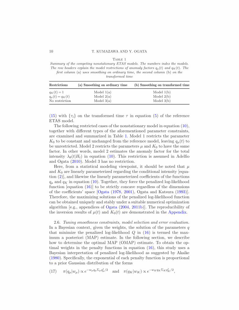
Table 1
Summary of the competing nonstationary ETAS models. The numbers index the models.The row headers explain the model restrictions of anomaly factors qµ(t) and qK(t). The
first column (a) uses smoothing on ordinary time, the second column (b) on thetransformed time
Restrictions (a) Smoothing on ordinary time (b) Smoothing on transformed time
qK(t) = 1 Model 1(a) Model 1(b)qµ(t) = qK(t) Model 2(a) Model 2(b)No restriction Model 3(a) Model 3(b)
(15) with {τi} on the transformed time τ in equation (5) of the referenceETAS model.
The following restricted cases of the nonstationary model in equation (10),together with different types of the aforementioned parameter constraints,are examined and summarized in Table 1. Model 1 restricts the parameterK0 to be constant and unchanged from the reference model, leaving qµ(t) tobe unrestricted. Model 2 restricts the parameters µ and K0 to have the samefactor. In other words, model 2 estimates the anomaly factor for the totalintensity λθ(t|Ht) in equation (10). This restriction is assumed in Adelfioand Ogata (2010). Model 3 has no restriction.
Here, from a statistical modeling viewpoint, it should be noted that µand K0 are linearly parameterized regarding the conditional intensity [equa-tion (2)], and likewise the linearly parameterized coefficients of the functionsqµ and qK in equation (10). Together, they force the penalized log-likelihoodfunction [equation (16)] to be strictly concave regardless of the dimensionsof the coefficients’ space [Ogata (1978, 2001), Ogata and Katsura (1993)].Therefore, the maximizing solutions of the penalized log-likelihood functioncan be obtained uniquely and stably under a suitable numerical optimizationalgorithm [e.g., appendices of Ogata (2004, 2011b)]. The reproducibility ofthe inversion results of µ(t) and K0(t) are demonstrated in the Appendix.
2.6. Tuning smoothness constraints, model selection and error evaluation.
In a Bayesian context, given the weights, the solution of the parameters qthat minimize the penalized log-likelihood Q in (16) is termed the max-imum a posteriori (MAP) estimate. In the following section, we describehow to determine the optimal MAP (OMAP) estimate. To obtain the op-timal weights in the penalty functions in equation (16), this study uses aBayesian interpretation of penalized log-likelihood as suggested by Akaike(1980). Specifically, the exponential of each penalty function is proportionalto a prior Gaussian distribution of the forms
π(qµ|wµ)∝ e−wµqµΣµqtµ/2 and π(qK |wK)∝ e−wKqKΣKqtK/2,(17)
NONSTATIONARY ETAS MODELS 11
since the coefficients of the function q.(·) in the penalty term Φ take aquadratic form with a symmetric (N + 1) × (N + 1) nonnegative definitematrix Σ. Since each matrix Σ is degenerate and has rank(Σ) =N , aboveeach prior distribution becomes improper [Ogata and Katsura (1993)]. Toavoid such improper priors, we divide each of the vectors q into (qc, q(N+1))so that each of the priors becomes a probability density function with respectto qc:
π(qc|w,qN+1) =(wN detΣc)1/2
√2π
Nexp
(
−1
2wNqcΣctqc
)
,(18)
where Σc is the cofactor of the last diagonal element of Σ, and w and q(N+1)
are considered hyperparameters to maximize the integral of the posteriordistribution with respect to qc,
Ψ(wµ,wK ; q(N+1)µ , q
(N+1)K )
(19)
=
∫
L(qµ, qK)π(qµ|wµ)π(qK |wK)dqcµ dqcK ,
which refers to the likelihood of a Bayesian model. Good (1965) suggeststhe maximization of equation (19) with respect to the hyperparameters andtermed this the Type II maximum likelihood procedure.
By applying Laplace’s method [Laplace (1774), pages 366–367], the pos-terior distribution is approximated by a Gaussian distribution, by which theintegral in equation (19) becomes
Ψ(wµ,wK ; q(N+1)µ , q
(N+1)K )
=Q(qcµ, qcK |wµ,wK ; q(N+1)
µ , q(N+1)K )(20)
− 12 log(detHµ)− 1
2 log(detHK) +MN log 2π,
where q is the maximum of the penalized log-likelihood Q in equation (16)and
H(qc|w,q(N+1)) =∂2 logL(qc|w,q(N+1))
∂qc ∂(qc)t−Σc(w,q(N+1)),(21)
for a fixed weight w for either wµ or wK .Thus, maximizing equation (16) with respect to qc and equation (20) with
respect to (wµ,wK ; q(N+1)µ , q
(N+1)K ), in turn, achieves our objective. In the for-
mer maximization, a quasi-Newton method using the gradients ∂ logL(q)/∂qand the Newton method making use of the Hessian matrices, equation (21),endure a fast convergence regardless of high dimensions. For the latter max-imization, a direct search such as the simplex method is used. A flowchart ofnumerical algorithms is described in the appendices of Ogata (2004, 2011b).
12 T. KUMAZAWA AND Y. OGATA
Anomaly factor functions under the optimal roughness penalty result insuitably smooth curves throughout the period. Furthermore, there may be achange point that results in sudden changes in parameters µ or K. To exam-ine such a discontinuity, a sufficiently small weight is put into the intervalthat includes a change point (e.g., w = 10−5), and the goodness-of-fit byABIC is compared with that of the smooth model with the optimal weightsfor all intervals.
It is useful to obtain the estimation error bounds of the MAP estimate qat each time of an observed earthquake. The joint error distribution of theparameters at q is nearly a 2N -dimensional normal distribution N(0,H−1),
where H−1 = (hi,j), and H = (hi,j) is the Hessian matrix in equation (21).Hence, the covariance function of the error process becomes
c(u, v) =2N∑
i=1
2N∑
j=1
Fi(u)hi,jFj(v),(22)
where Fi = FN+i for i= 1,2, . . . ,N , which is defined in equation (13). Thus,the standard error of q is provided by
ε(t) = [εµ(t), εK(t)] =√
C(t, t).(23)
2.7. Bayesian model comparison. It is necessary to compare the good-ness of fit among the competing models. From equation (20), the ABIC
[Akaike (1980)] can be obtained as
ABIC = (−2) maxwµ,wK ;q
(N+1)µ ,q
(N+1)K
logΨ(wµ,wK ; q(N+1)µ , q
(N+1)K )
(24)+ 2× (#hyperparameter).
Specifically, models 1 and 2 [1(a) and (b), 2(a) and (b) in Table 1] have fourhyperparameters, and model 3 [3(a) and (b)] has eight. A Bayesian modelwith the smallest ABIC value provides the best fit to the data.
Since there are various constraints in the different setups, the resultingABIC values cannot be simply compared because of unknown different con-stants, mainly due to the approximations in equation (20). Alternatively, thedifference of ABIC values relative to those corresponding to the referencemodel are used. In other words, the reduction amount of the ABIC valuefrom a very heavily constrained case,
∆ABIC =ABIC −ABIC 0,(25)
where ABIC is that of equation (24) and ABIC 0 is the ABIC value withvery heavy fixed weights, which constrain the function to be almost constant.Therefore, the ∆ABIC approximates the ABIC improvement from the flatanomaly functions [q(t) = 1 for all t] to the optimal functions.
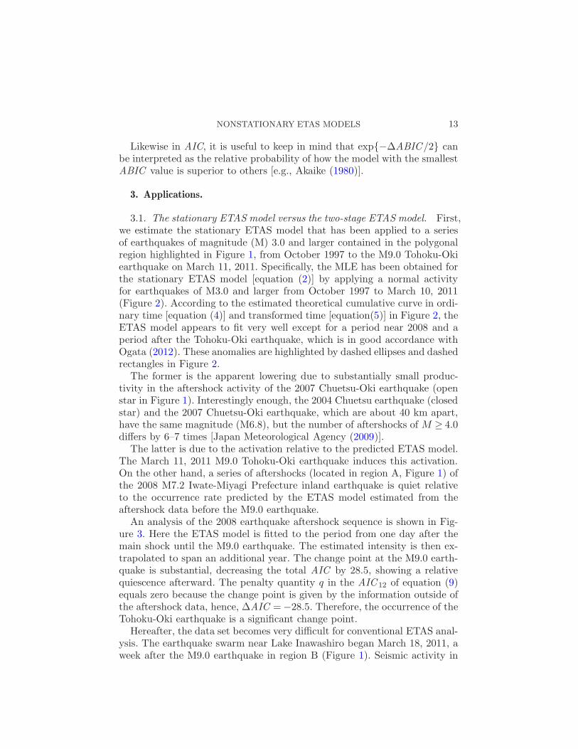
NONSTATIONARY ETAS MODELS 13
Likewise in AIC, it is useful to keep in mind that exp{−∆ABIC/2} canbe interpreted as the relative probability of how the model with the smallestABIC value is superior to others [e.g., Akaike (1980)].
3. Applications.
3.1. The stationary ETAS model versus the two-stage ETAS model. First,we estimate the stationary ETAS model that has been applied to a seriesof earthquakes of magnitude (M) 3.0 and larger contained in the polygonalregion highlighted in Figure 1, from October 1997 to the M9.0 Tohoku-Okiearthquake on March 11, 2011. Specifically, the MLE has been obtained forthe stationary ETAS model [equation (2)] by applying a normal activityfor earthquakes of M3.0 and larger from October 1997 to March 10, 2011(Figure 2). According to the estimated theoretical cumulative curve in ordi-nary time [equation (4)] and transformed time [equation(5)] in Figure 2, theETAS model appears to fit very well except for a period near 2008 and aperiod after the Tohoku-Oki earthquake, which is in good accordance withOgata (2012). These anomalies are highlighted by dashed ellipses and dashedrectangles in Figure 2.
The former is the apparent lowering due to substantially small produc-tivity in the aftershock activity of the 2007 Chuetsu-Oki earthquake (openstar in Figure 1). Interestingly enough, the 2004 Chuetsu earthquake (closedstar) and the 2007 Chuetsu-Oki earthquake, which are about 40 km apart,have the same magnitude (M6.8), but the number of aftershocks of M ≥ 4.0differs by 6–7 times [Japan Meteorological Agency (2009)].
The latter is due to the activation relative to the predicted ETAS model.The March 11, 2011 M9.0 Tohoku-Oki earthquake induces this activation.On the other hand, a series of aftershocks (located in region A, Figure 1) ofthe 2008 M7.2 Iwate-Miyagi Prefecture inland earthquake is quiet relativeto the occurrence rate predicted by the ETAS model estimated from theaftershock data before the M9.0 earthquake.
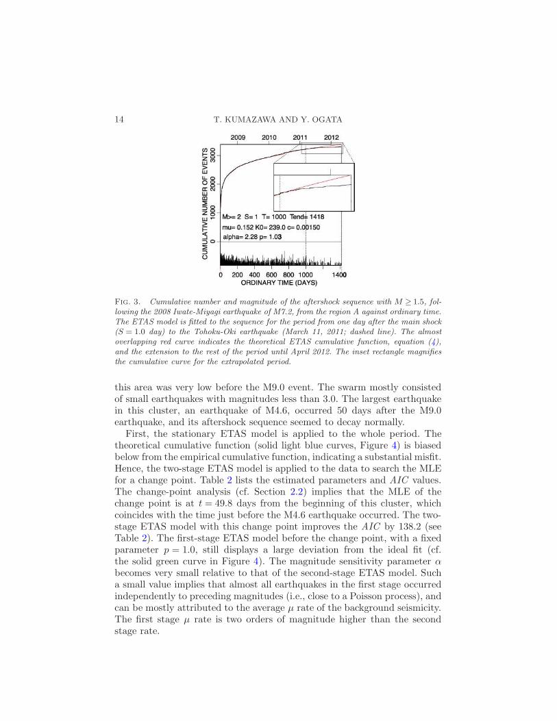
An analysis of the 2008 earthquake aftershock sequence is shown in Fig-ure 3. Here the ETAS model is fitted to the period from one day after themain shock until the M9.0 earthquake. The estimated intensity is then ex-trapolated to span an additional year. The change point at the M9.0 earth-quake is substantial, decreasing the total AIC by 28.5, showing a relativequiescence afterward. The penalty quantity q in the AIC 12 of equation (9)equals zero because the change point is given by the information outside ofthe aftershock data, hence, ∆AIC =−28.5. Therefore, the occurrence of theTohoku-Oki earthquake is a significant change point.
Hereafter, the data set becomes very difficult for conventional ETAS anal-ysis. The earthquake swarm near Lake Inawashiro began March 18, 2011, aweek after the M9.0 earthquake in region B (Figure 1). Seismic activity in
14 T. KUMAZAWA AND Y. OGATA
Fig. 3. Cumulative number and magnitude of the aftershock sequence with M ≥ 1.5, fol-lowing the 2008 Iwate-Miyagi earthquake of M7.2, from the region A against ordinary time.The ETAS model is fitted to the sequence for the period from one day after the main shock(S = 1.0 day) to the Tohoku-Oki earthquake (March 11, 2011; dashed line). The almostoverlapping red curve indicates the theoretical ETAS cumulative function, equation (4),and the extension to the rest of the period until April 2012. The inset rectangle magnifiesthe cumulative curve for the extrapolated period.
this area was very low before the M9.0 event. The swarm mostly consistedof small earthquakes with magnitudes less than 3.0. The largest earthquakein this cluster, an earthquake of M4.6, occurred 50 days after the M9.0earthquake, and its aftershock sequence seemed to decay normally.
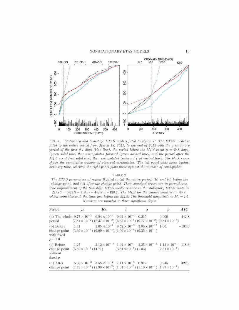
First, the stationary ETAS model is applied to the whole period. Thetheoretical cumulative function (solid light blue curves, Figure 4) is biasedbelow from the empirical cumulative function, indicating a substantial misfit.Hence, the two-stage ETAS model is applied to the data to search the MLEfor a change point. Table 2 lists the estimated parameters and AIC values.The change-point analysis (cf. Section 2.2) implies that the MLE of thechange point is at t = 49.8 days from the beginning of this cluster, whichcoincides with the time just before the M4.6 earthquake occurred. The two-stage ETAS model with this change point improves the AIC by 138.2 (seeTable 2). The first-stage ETAS model before the change point, with a fixedparameter p = 1.0, still displays a large deviation from the ideal fit (cf.the solid green curve in Figure 4). The magnitude sensitivity parameter αbecomes very small relative to that of the second-stage ETAS model. Sucha small value implies that almost all earthquakes in the first stage occurredindependently to preceding magnitudes (i.e., close to a Poisson process), andcan be mostly attributed to the average µ rate of the background seismicity.The first stage µ rate is two orders of magnitude higher than the secondstage rate.
NONSTATIONARY ETAS MODELS 15
Fig. 4. Stationary and two-stage ETAS models fitted to region B. The ETAS model isfitted to the entire period from March 18, 2011, to the end of 2012 with the preliminaryperiod of the first 0.1 days (blue line), the period before the M4.6 event (t = 49.8 days)(green solid line) then extrapolated forward (green dashed line), and the period after theM4.6 event (red solid line) then extrapolated backward (red dashed line). The black curveshows the cumulative number of observed earthquakes. The left panel plots these againstordinary time, whereas the right panel plots these against the number of earthquakes.
Table 2
The ETAS parameters of region B fitted to (a) the entire period, (b) and (c) before thechange point, and (d) after the change point. Their standard errors are in parentheses.The improvement of the two-stage ETAS model relative to the stationary ETAS model is∆AIC = (422.9− 118.3)− 442.8 =−138.2. The MLE for the change point is t= 49.8,
which coincides with the time just before the M4.6. The threshold magnitude is Mz = 2.5.Numbers are rounded to three significant digits
Period µ K0 c α p AIC
(a) The whole 9.77× 10⁻² 6.54× 10⁻² 9.64× 10⁻⁴ 0.215 0.900 442.8period (7.81×10⁻²) (2.37×10⁻²) (6.35×10⁻⁴) (9.77×10⁻²) (9.84×10⁻³)
(b) Before 1.41 1.05× 10⁻¹ 8.52× 10⁻² 3.06×10⁻¹⁵ 1.00 −103.0change point (3.39×10⁻¹) (6.99×10⁻²) (1.09×10⁻¹) (9.35×10⁻¹)with fixedp= 1.0
(c) Before 1.27 2.12×10+11 1.04× 10+1 2.25×10⁻¹² 1.13× 10+1 −118.3change point (5.52×10⁻¹) (4.71) (3.81×10⁻¹) (1.03) (2.31×10⁻¹)withoutfixed p
(d) After 6.58× 10⁻² 3.58× 10⁻² 7.11× 10⁻⁵ 0.912 0.945 422.9change point (1.43×10⁻¹) (1.90×10⁻²) (1.01×10⁻³) (1.10×10⁻¹) (1.87×10⁻¹)
16 T. KUMAZAWA AND Y. OGATA
If p is not fixed, the estimated K0, c and p have extremely large valuesfor a normal earthquake sequence while α approaches zero. Consequently,the model is again approximate to a nonstationary Poisson process, char-acterizing the sequence as a swarm, with an AIC smaller than that of thep = 1.0 scenario. The large discrepancies between the estimated parametervalues between (b) and (c) in Table 2 suggest that the stationary ETASmodel is not well defined for this particular earthquake sequence in the firstperiod before the change point. The standard errors for the parameter α aremultiple orders of magnitude greater than those of the estimates themselves.The narrow magnitude range makes it difficult for the model to distinguishthe effects of K0 and α, causing a trade-off between these two parameters,thus providing inaccurate estimations. For the case without a fixed p, theaftershock productivity K0 becomes extremely small in compensation forthe small α estimate.
After the change-point time of the M4.6 earthquake, the ETAS model fitsconsiderably well for several months. Then, a deviation becomes noticeablerelative to the solid red cumulative curve in Figure 4. From these observa-tions, it is concluded that the M4.6 earthquake has reduced swarm activityand that decaying normal aftershock type activity has dominated.
3.2. Comparison of the nonstationary models. In this section the pro-posed nonstationary models and methods outlined in Sections 2.4–2.6 areapplied to the same data from region B near Lake Inawashiro. To replicatethe transient nonstationary activities in this particular region, we use theseismic activity in the larger polygonal region in Figure 1 for the periodbefore the M9.0 earthquake (MLEs are shown in Figure 2). Such a referencemodel represents a typical seismicity pattern over a wide region throughoutthe period, and therefore represents a robust estimate against the inclusionof local and transient anomalies.
By fixing the reference parameters c,α and p, both in the stationary andtwo-stage ETAS models, µ and K0 are estimated for events from region Bafter the M9.0 event, with a magnitude M ≥ 2.5. Table 3 summarizes there-estimated parameters, together with the corresponding AIC values. TheAIC improvement of the two-stage ETAS model is 126.2.
Next, we have applied the nonstationary ETAS models listed in Table 1,with and without a change point taken into consideration, using the referenceparameters in the first row of Table 3. Here, if a change point of M4.6 atthe time t= 49.8 days occurs, we propose a very small fixed value such asthat described in Section 2.5.
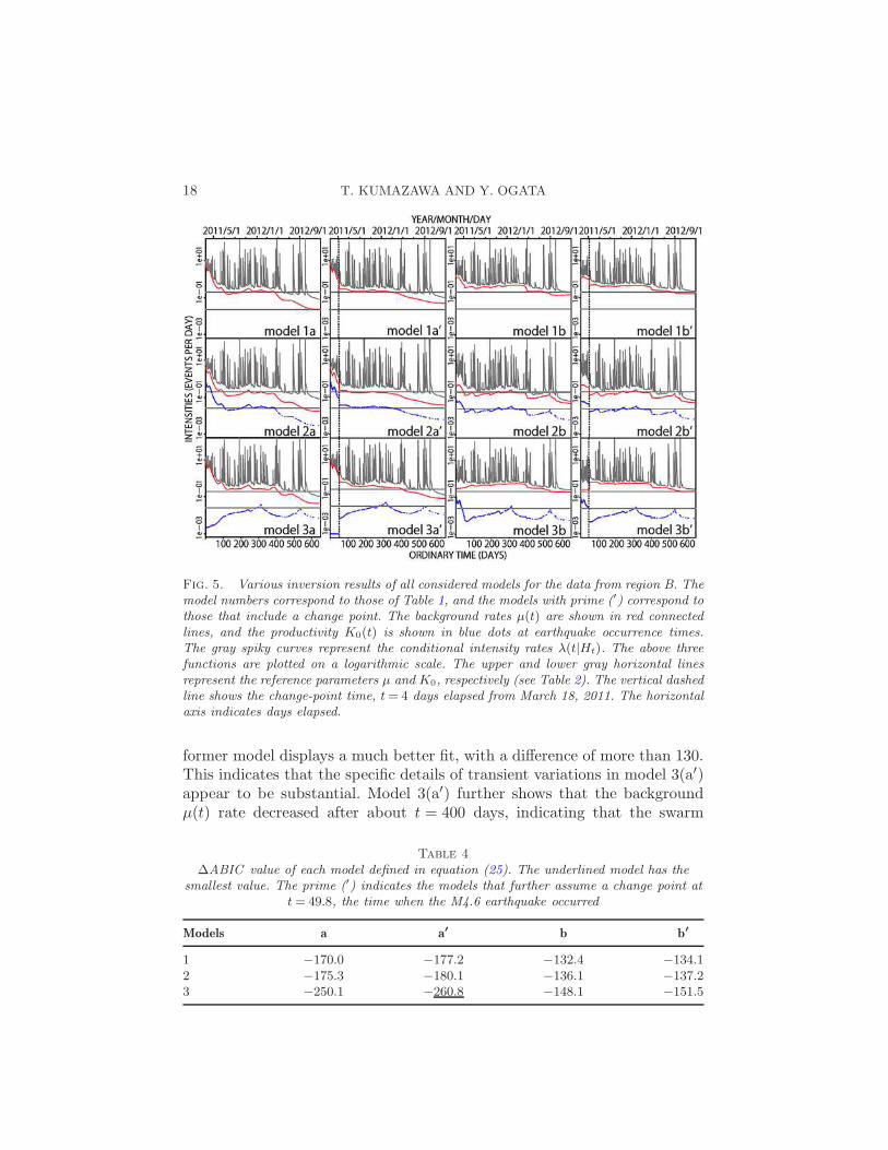
Figure 5 shows all of the inversion results (maximum posterior estimates)for a total of 12 models. The ∆ABIC values of the corresponding models aregiven in Table 4. Models with the change point outperform correspondingmodels without the change point. This highlights the significance of jumps
NONSTATIONARY ETAS MODELS 17
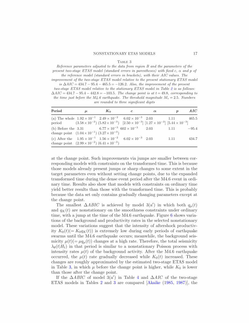
Table 3
Reference parameters adjusted to the data from region B and the parameters of thepresent two-stage ETAS model (standard errors in parentheses) with fixed c, α and p of
the reference model (standard errors in brackets), with their AIC values. Theimprovement of the two-stage ETAS model relative to the present stationary ETAS model
is ∆AIC = 434.7− 95.4− 465.5 =−126.2. Also, the improvement of the presenttwo-stage ETAS model relative to the stationary ETAS model in Table 2 is as follows:
∆AIC = 434.7− 95.4− 442.8 =−103.5. The change point is at t= 49.8, corresponding tothe time just before the M4.6 earthquake. The threshold magnitude Mz = 2.5. Numbers
are rounded to three significant digits
Period µ K0 c α p AIC
(a) The whole 1.92× 10⁻¹ 2.49× 10⁻² 6.02× 10⁻³ 2.03 1.11 465.5period (3.58×10⁻²) (5.82×10⁻³) [2.50× 10⁻³] [1.27× 10⁻²] [5.44× 10⁻³]
(b) Before the 3.31 6.77× 10⁻³ 602× 10−3 2.03 1.11 −95.4change point (1.04×10⁻¹) (3.27×10⁻³)
(c) After the 1.95× 10⁻¹ 1.56× 10⁻² 6.02× 10⁻³ 2.03 1.11 434.7change point (2.99×10⁻²) (6.41×10⁻³)
at the change point. Such improvements via jumps are smaller between cor-responding models with constraints on the transformed time. This is becausethose models already present jumps or sharp changes to some extent in thetarget parameters even without setting change points, due to the expandedtransformed time during the dense event period after the M4.6 event in ordi-nary time. Results also show that models with constraints on ordinary timeyield better results than those with the transformed time. This is probablybecause the data set only contains gradually changing parameters except atthe change point.
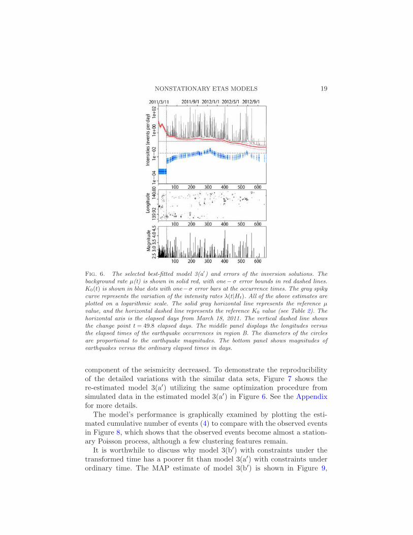
The smallest ∆ABIC is achieved by model 3(a′) in which both qµ(t)and qK(t) are nonstationary on the smoothness constraints under ordinarytime, with a jump at the time of the M4.6 earthquake. Figure 6 shows varia-tions of the background and productivity rates in the selected nonstationarymodel. These variations suggest that the intensity of aftershock productiv-ity K0(t)(= K0qK(t)) is extremely low during early periods of earthquakeswarms until the M4.6 earthquake occurs; meanwhile, the background seis-micity µ(t)(= µqµ(t)) changes at a high rate. Therefore, the total seismicityλθ(t|Ht) in that period is similar to a nonstationary Poisson process withintensity rates µ(t) of the background activity. After the M4.6 earthquakeoccurred, the µ(t) rate gradually decreased while K0(t) increased. Thesechanges are roughly approximated by the estimated two-stage ETAS modelin Table 3, in which µ before the change point is higher, while K0 is lowerthan those after the change point.
If the ∆ABIC of model 3(a′) in Table 4 and ∆AIC of the two-stageETAS models in Tables 2 and 3 are compared [Akaike (1985, 1987)], the
18 T. KUMAZAWA AND Y. OGATA
Fig. 5. Various inversion results of all considered models for the data from region B. Themodel numbers correspond to those of Table 1, and the models with prime (′) correspond tothose that include a change point. The background rates µ(t) are shown in red connectedlines, and the productivity K0(t) is shown in blue dots at earthquake occurrence times.The gray spiky curves represent the conditional intensity rates λ(t|Ht). The above threefunctions are plotted on a logarithmic scale. The upper and lower gray horizontal linesrepresent the reference parameters µ and K0, respectively (see Table 2). The vertical dashedline shows the change-point time, t= 4 days elapsed from March 18, 2011. The horizontalaxis indicates days elapsed.
former model displays a much better fit, with a difference of more than 130.This indicates that the specific details of transient variations in model 3(a′)appear to be substantial. Model 3(a′) further shows that the backgroundµ(t) rate decreased after about t = 400 days, indicating that the swarm
Table 4
∆ABIC value of each model defined in equation (25). The underlined model has thesmallest value. The prime (′) indicates the models that further assume a change point at
t= 49.8, the time when the M4.6 earthquake occurred
Models a a′ b b′
1 −170.0 −177.2 −132.4 −134.12 −175.3 −180.1 −136.1 −137.23 −250.1 −260.8 −148.1 −151.5
NONSTATIONARY ETAS MODELS 19
Fig. 6. The selected best-fitted model 3(a′) and errors of the inversion solutions. Thebackground rate µ(t) is shown in solid red, with one− σ error bounds in red dashed lines.K0(t) is shown in blue dots with one−σ error bars at the occurrence times. The gray spikycurve represents the variation of the intensity rates λ(t|Ht). All of the above estimates areplotted on a logarithmic scale. The solid gray horizontal line represents the reference µ
value, and the horizontal dashed line represents the reference K0 value (see Table 2). Thehorizontal axis is the elapsed days from March 18, 2011. The vertical dashed line showsthe change point t = 49.8 elapsed days. The middle panel displays the longitudes versusthe elapsed times of the earthquake occurrences in region B. The diameters of the circlesare proportional to the earthquake magnitudes. The bottom panel shows magnitudes ofearthquakes versus the ordinary elapsed times in days.
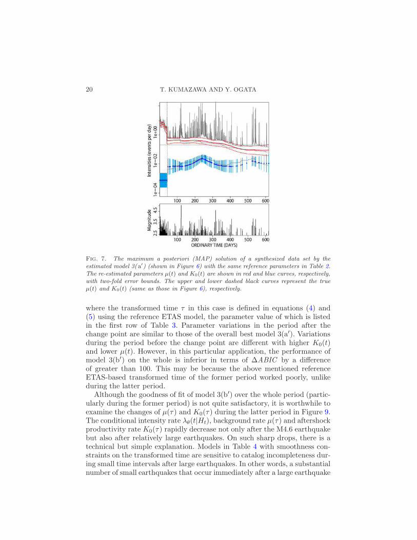
component of the seismicity decreased. To demonstrate the reproducibilityof the detailed variations with the similar data sets, Figure 7 shows there-estimated model 3(a′) utilizing the same optimization procedure fromsimulated data in the estimated model 3(a′) in Figure 6. See the Appendixfor more details.
The model’s performance is graphically examined by plotting the esti-mated cumulative number of events (4) to compare with the observed eventsin Figure 8, which shows that the observed events become almost a station-ary Poisson process, although a few clustering features remain.
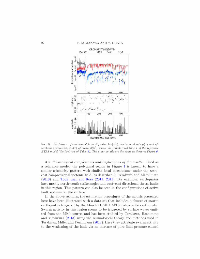
It is worthwhile to discuss why model 3(b′) with constraints under thetransformed time has a poorer fit than model 3(a′) with constraints underordinary time. The MAP estimate of model 3(b′) is shown in Figure 9,
20 T. KUMAZAWA AND Y. OGATA
Fig. 7. The maximum a posteriori (MAP) solution of a synthesized data set by theestimated model 3( a′) (shown in Figure 6) with the same reference parameters in Table 2.The re-estimated parameters µ(t) and K0(t) are shown in red and blue curves, respectively,with two-fold error bounds. The upper and lower dashed black curves represent the trueµ(t) and K0(t) (same as those in Figure 6), respectively.
where the transformed time τ in this case is defined in equations (4) and(5) using the reference ETAS model, the parameter value of which is listedin the first row of Table 3. Parameter variations in the period after thechange point are similar to those of the overall best model 3(a′). Variationsduring the period before the change point are different with higher K0(t)and lower µ(t). However, in this particular application, the performance ofmodel 3(b′) on the whole is inferior in terms of ∆ABIC by a differenceof greater than 100. This may be because the above mentioned referenceETAS-based transformed time of the former period worked poorly, unlikeduring the latter period.
Although the goodness of fit of model 3(b′) over the whole period (partic-ularly during the former period) is not quite satisfactory, it is worthwhile toexamine the changes of µ(τ) and K0(τ) during the latter period in Figure 9.The conditional intensity rate λθ(t|Ht), background rate µ(τ) and aftershockproductivity rate K0(τ) rapidly decrease not only after the M4.6 earthquakebut also after relatively large earthquakes. On such sharp drops, there is atechnical but simple explanation. Models in Table 4 with smoothness con-straints on the transformed time are sensitive to catalog incompleteness dur-ing small time intervals after large earthquakes. In other words, a substantialnumber of small earthquakes that occur immediately after a large earthquake

NONSTATIONARY ETAS MODELS 21
Fig. 8. Estimated cumulative number of events by model 3( a′) (red curves) and theobserved number of events (black curve) for the ordinary time (top panel) and residual time(bottom panel). Gray circles show the depths of the swarm events versus the correspondingtime.
are missing in the earthquake catalog [e.g., Ogata and Katsura (2006); Omiet al. (2013)]. Present results suggest that the smoothing on the transformedtime can be used as a supplemental tool to check catalog completeness. Thetime transformation stretches out ordinary time where the intensity rate ishigh and, hence, transforming the smoothed parameters back to ordinarytime can result in sharp changes. This type of constraint can be useful fordifferent applications in which occasional rapid changes are expected.
22 T. KUMAZAWA AND Y. OGATA
Fig. 9. Variations of conditional intensity rates λ(τ |Hτ ), background rate µ(τ ) and af-tershock productivity K0(τ ) of model 3(b′) versus the transformed time τ of the referenceETAS model (the first row of Table 3). The other details are the same as those in Figure 6.
3.3. Seismological complements and implications of the results. Used asa reference model, the polygonal region in Figure 1 is known to have asimilar seismicity pattern with similar focal mechanisms under the west–east compressional tectonic field, as described in Terakawa and Matsu’uara(2010) and Toda, Lian and Ross (2011, 2011). For example, earthquakeshave mostly north–south strike angles and west–east directional thrust faultsin this region. This pattern can also be seen in the configurations of activefault systems on the surface.
In the above sections, the estimation procedures of the models presentedhere have been illustrated with a data set that includes a cluster of swarmearthquakes triggered by the March 11, 2011 M9.0 Tohoku-Oki earthquake.Swarm activity in this region seems to be triggered by surface waves emit-ted from the M9.0 source, and has been studied by Terakawa, Hashimotoand Matsu’ura (2013) using the seismological theory and methods used inTerakawa, Miller and Deichmann (2012). Here they attribute swarm activityto the weakening of the fault via an increase of pore fluid pressure caused
NONSTATIONARY ETAS MODELS 23
by the dynamic triggering effect due to surface waves of the Tohoku-Okirapture. Thus, the initially very high and then decreasing rate of µ(t) re-flects changes in fault strength, probably due to the intrusion and decreasein pore fluid pressure. The analyses presented here support the quantitative,phenomenological evidence of fault weakening via the intrusion of water intothe fault system in earlier periods [Terakawa, Miller and Deichmann (2012,2013)]. Similarly, by monitoring swarm activity, this nonstationary modelcan be expected to make quantitative inferences of magma intrusions anddraining during volcanic activity.
The background seismicity parameter in the ETAS model is sensitiveto transient aseismic phenomena such as slow slips (quiet earthquakes) onand around tectonic plate boundaries [Llenos, Mcguire and Ogata (2009),Okutani and Ide (2011)]. This could possibly link a given swarm activity tothe weakening of interfaces. Changes in the pore fluid pressure, for example,alter the friction rate of fault interfaces, thereby changing the fault strength.Hence, monitoring the changes in background seismicity has the potentialto detect such aseismic events.
Changes in the aftershock productivity K0, on the other hand, appear todepend on the locations of earthquake clusters and appear to vary amongclusters where secondary aftershocks are conspicuous. The aftershock pro-ductivity K0 therefore reflects the geology around faults rather than thechanges in stress rate. The application of the space–time ETAS model withlocation-dependent parameters [e.g., Ogata, Katsura and Tanemura (2003),Ogata (2004, 2011b)] reveals that the K0 function varies (i.e., location sen-sitive) unlike other parameters. Still, the task remains to confirm the linkbetween the changes in ETAS parameters and physical processes happeningon and around faults.
4. Conclusions and discussion. There are many examples in seismologyin which different authors have obtained differing inversion results for thesame scientific phenomenon. These differences are attributed to the adop-tion of different priors for the parameters of a given model. Scenarios inthis study have the same problem and are highlighted in Figure 5. Modelparameters in this study are estimated by maximizing the penalized log like-lihood, which is intrinsically nonlinear. Besides adjusting the weights in thepenalty (namely, hyperparameters of a prior distribution), it is necessary tocompare the adequacy of different penalties (prior distributions) associatedwith the same likelihood function. For these purposes, we have proposed theobjective procedure using ∆ABIC and ∆AIC .
A suitable ETAS model [equation (2)] is first established with MLE asthe reference predictive model to monitor future seismic activity and to de-tect anomalous seismic activity. Sometimes, transient activity starts in a
24 T. KUMAZAWA AND Y. OGATA
region with very low seismicity. In such a case, it is both practical and ap-plicable to use a data set from a wider region to estimate the stable androbust parameter values of c, α and p in the ETAS model [equation (2)].Then, the competing nonstationary ETAS models in equation (10) are fittedtogether with constraint functions in equations (11) and (12) using eitherordinary time or transformed time to penalize the time-dependent parame-ters in the models. The corresponding Bayesian models include a differentprior distribution of the anomaly factor coefficients qµ(·) and qK(·), whichare functions of either the ordinary time t [models 1(a)–3(a) in Table 1] orthe transformed time τ in the reference ETAS model [models 1(b)–3(b)].Furthermore, models in which the anomaly functions involve a discontinu-ity [models 1(a′)–3(a′) and 1(b′)–3(b′)] are considered. Using the ∆ABIC
value, the goodness-of-fit performances of all of the different models aresummarized in Table 4. Among the competing models, model 3(a′) attainedthe smallest ∆ABIC value, and it is therefore concluded that this modelprovides the best inversion result for this particular data set.
Thus, changes in background seismicity µ and/or aftershock productivityK0 of the ETAS model can be monitored. The background seismicity rate inthe ETAS models represents a portion of the occurrence rate due to externaleffects that are not included in the observed earthquake occurrence history inthe focal region of interest. Therefore, changes in the background rate havebeen attracting the interest of many researchers because such changes aresometimes precursors to large earthquakes. The declustering algorithms [e.g.,Reasenberg (1985), Zhuang, Ogata and Vere-Jones (2002, 2004)] have beenadopted to determine the background seismicity by stochastically removingthe clustering components depending on the ratio of the background rate tothe whole intensity at each occurrence time. The change-point analysis andnonstationary models presented in this study, however, objectively serve amore quantitatively explicit way to approach this task.
The case where the other three parameters c,α and p in equation (2)also vary with time was not examined in this study. For example, in Fig-ure 8, we have seen that the best model in our framework does not captureall of the clustering events but misses a few small clusters, which suggeststhe time dependency of the parameters. For another example, we have seenthe effect of missing earthquakes in Figure 7, suggesting that parameter cmay depend on the magnitude of the earthquake, leading to a significantcorrelation between c and p. Furthermore, in Section 2.3, it is mentionedthat K0 is correlated with the parameter α. Unstable estimations of K0 andthe α value in the swarm period before the M4.6 earthquake can be seenin Table 2, during which period most of the magnitudes are between 2.5and 3. This is another reason why the α value is fixed by the correspondingreference parameter α when the nonstationary models are applied. Owing
NONSTATIONARY ETAS MODELS 25
to the linearly parameterized coefficients of the functions qµ and qK in equa-tion (10), the maximizing solutions of the penalized log-likelihood function[equation (16)], in spite of the high dimension, can be obtained uniquely andstably by fixing the three parameters c,α and p.
APPENDIX: SYNTHETIC TEST OF REPRODUCIBILITY OFNONSTATIONARY PATTERNS
We tested our method with synthetic data sets to check if both µ(t) andK0(t) can be reproduced by simulated data sets that are similar to observeddata sets. We used the reference parameter set (Table 2) with the bestestimated µ(t) and K0(t) of model 3(a′).
The magnitude sequence of the synthetic data was generated on the basisof the Gutenberg–Richter law with a b-value of the original data set (b =1.273). In other words, the magnitude of each earthquake will independentlyobey an exponential distribution such that f(M) = β exp{−β(M − Mc),M ≥ Mc, where β = b ln 10, and Mc = 2.5 is the magnitude value abovewhich all earthquakes are detected.
The thinning method [Ogata (1981, 1998)] is adopted for data simulation.A total of 470 events were simulated with a threshold magnitude of 2.5.Model 3(a′) was then fitted to the simulated data sets, with a change pointat the same time as the original data (between the 182nd and 183rd event).Results are shown in Figure 7; the estimated µ(t) and K0(t) appear to besimilar to the original µ(t) and K0(t) in Figure 6, respectively, within a 2σerror.
Acknowledgments. We are grateful to the Japan Meteorological Agency(JMA), the National Research Institute for Earth Science and Disaster Pre-vention (NIED) and the universities for the hypocenter data. We used theTSEIS visualization program package [Tsuruoka (1996)] for the study ofhypocenter data.
REFERENCES
Adelfio, G. and Ogata, Y. (2010). Hybrid kernel estimates of space–time earthquakeoccurrence rates using the epidemic-type aftershock sequence model. Ann. Inst. Statist.Math. 62 127–143. MR2577443
Akaike, H. (1973). Information theory and an extension of the maximum likelihood prin-ciple. In Second International Symposium on Information Theory (Tsahkadsor, 1971)267–281. Akademiai Kiado, Budapest. MR0483125
Akaike, H. (1974). A new look at the statistical model identification. IEEE Trans.Automat. Control AC-19 716–723. System identification and time-series analysis.MR0423716
Akaike, H. (1977). On entropy maximization principle. In Applications of Statistics(P. R. Krishnaian, ed.) 27–41. North-Holland, Amsterdam. MR0501456
26 T. KUMAZAWA AND Y. OGATA
Akaike, H. (1980). Likelihood and the Bayes procedure. In Bayesian Statistics (Valencia,1979) (J. M. Bernardo, M. H. De Groot, D. V. Lindley and A. F. M. Smith,eds.) 143–166. Univ. Press, Valencia, Spain. MR0638876
Akaike, H. (1985). Prediction and entropy. In A Celebration of Statistics (A. C. Atkin-
son and E. Fienberg, eds.) 1–24. Springer, New York. MR0816143Akaike, H. (1987). Factor analysis and AIC. Psychometrika 52 317–332. MR0914459Balderama, E., Paik Schoenberg, F., Murray, E. and Rundel, P. W. (2012). Ap-
plication of branching models in the study of invasive species. J. Amer. Statist. Assoc.107 467–476. MR2980058
Bansal, A. R. and Ogata, Y. (2013). A non-stationary epidemic type aftershock se-quence model for seismicity prior to the December 26, 2004 M9.1 Sumatra-AndamanIslands mega-earthquake. J. Geophys. Res. 118 616–629.
Chavez-Demoulina, V. and Mcgillb, J. A. (2012). High-frequency financial data mod-eling using Hawkes processes. J. Bank. Financ. 36 3415–3426.
Daley, D. and Vere-Jones, D. (2003). An Introduction to the Theory of Point Processes,2nd ed. Springer, New York.
Good, I. J. (1965). The Estimation of Probabilities. An Essay on Modern Bayesian Meth-ods. MIT Press, Cambridge, MA. MR0185724
Good, I. J. and Gaskins, R. A. (1971). Nonparametric roughness penalties for proba-bility densities. Biometrika 58 255–277. MR0319314
Hainzl, S. and Ogata, Y. (2005). Detecting fluid signals in seismicity data throughstatistical earthquake modeling. J. Geophys. Res. 110 B5, B05S07.
Hassan Zadeh, A. and Sharda, R. (2012). Modeling brand post popularity in onlinesocial networks. Social Science Research Network. Available at SSRN 2182711.
Hawkes, A. G. (1971). Spectra of some self-exciting and mutually exciting point pro-cesses. Biometrika 58 83–90. MR0278410
Hawkes, A. G. and Adamopoulos, L. (1973). Cluster models for earthquakes—regionalcomparisons. Bull. Int. Stat. Inst. 45 454–461.
Hawkes, A. G. and Oakes, D. (1974). A cluster process representation of a self-excitingprocess. J. Appl. Probab. 11 493–503. MR0378093
Herrera, R. and Schipp, B. (2009). Self-exciting extreme value models for stock marketcrashes. In Statistical Inference, Econometric Analysis and Matrix Algebra 209–231.Physica-Verlag HD, Heidelberg.
Japan Meteorological Agency (2009). The Iwate-Miyagi Nairiku earthquake in 2008.Rep. Coord. Comm. Earthq. Predict 81 101–131. Available at http://cais.gsi.go.jp/YOCHIREN/report/kaihou81/03_04.pdf.
Jordan, T. H., Chen, Y.-T. and Gasparini, P. (2012). Operational earthquake fore-casting. State of knowledge and guidelines for utilization. Ann. Geophys. 54 315–391.
Kagan, Y. Y. and Knopoff, L. (1987). Statistical short-term earthquake prediction.Science 236 1563–1567.
Kendall, D. G. (1949). Stochastic processes and population growth. J. Roy. Statist. Soc.Ser. B. 11 230–264. MR0034977
Kumazawa, T., Ogata, Y. and Toda, S. (2010). Precursory seismic anomalies andtransient crustal deformation prior to the 2008 Mw = 6.9 Iwate-Miyagi Nairiku, Japan,earthquake. J. Geophys. Res. 115 B10312.
Laplace, P. S. (1774). Memoir on the probability of causes of events. Memoires demathematique et de physique, tome sixieme (English translation by S. M. Stigler, 1986).Statist. Sci. 1 364–378.
Llenos, A. L., Mcguire, J. J. andOgata, Y. (2009). Modeling seismic swarms triggeredby aseismic transients. Earth Planet. Sci. Lett. 281 59–69.
NONSTATIONARY ETAS MODELS 27
Lombardi, A. M., Cocco, M. and Marzocchi, W. (2010). On the increase of back-ground seismicity rate during the 1997–1998 Umbria–Marche, central Italy, sequence:
Apparent variation or fluid-driven triggering? Bull. Seismol. Soc. Amer. 100 1138–1152.Lomnitz, C. (1974). Global Tectonic and Earthquake Risk. Elsevier, Amsterdam.Mohler, G. O., Short, M. B., Brantingham, P. J., Schoenberg, F. P. and
Tita, G. E. (2011). Self-exciting point process modeling of crime. J. Amer. Statist.Assoc. 106 100–108. MR2816705
Ogata, Y. (1978). The asymptotic behaviour of maximum likelihood estimators for sta-tionary point processes. Ann. Inst. Statist. Math. 30 243–261. MR0514494
Ogata, Y. (1981). On Lewis’ simulation method for point processes. IEEE Trans. Inform.
Theory 27 23–31.Ogata, Y. (1985). Statistical models for earthquake occurrences and residual analysis for
point processes. Research Memorandum No. 388 (21 May), The Institute of StatisticalMathematics, Tokyo. Available at http://www.ism.ac.jp/editsec/resmemo-e.html.
Ogata, Y. (1986). Statistical models for earthquake occurrences and residual analysis for
point processes. Mathematical Seismology 1 228–281.Ogata, Y. (1988). Statistical models for earthquake occurrences and residual analysis for
point processes. J. Amer. Statist. Assoc. 83 9–27.Ogata, Y. (1989). Statistical model for standard seismicity and detection of anomalies
by residual analysis. Tectonophysics 169 159–174.
Ogata, Y. (1992). Detection of precursory relative quiescence before great earthquakesthrough a statistical model. J. Geophys. Res. 97 19845–19871.
Ogata, Y. (1998). Space–time point-process models for earthquake occurrences. Ann.Inst. Statist. Math. 50 379–402.
Ogata, Y. (1999). Seismicity analysis through point-process modeling: A review. Pure
Appl. Geophys. 155 471–507.Ogata, Y. (2001). Exploratory analysis of earthquake clusters by likelihood-based trigger
models. J. Appl. Probab. 38A 202–212. MR1915545Ogata, Y. (2004). Space–time model for regional seismicity and detection of crustal stress
changes. J. Geophys. Res. 109 B03308.
Ogata, Y. (2005). Detection of anomalous seismicity as a stress change sensor. J. Geophys.Res. 110 B05S06.
Ogata, Y. (2006a). Seismicity anomaly scenario prior to the major recurrent earthquakesoff the East coast of Miyagi prefecture, northern Japan. Tectonophysics 424 291–306.
Ogata, Y. (2006b). Fortran programs statistical analysis of seismicity—Updated version,
(SASeis2006). Computer Science Monograph No. 33, The Institute of Statistical Math-ematics, Tokyo, Japan. Available at http://www.ism.ac.jp/editsec/csm/index_j.
html.Ogata, Y. (2007). Seismicity and geodetic anomalies in a wide preceding the Niigata-Ken-
Chuetsu earthquake of 23 October 2004, central Japan. J. Geophys. Res. 112 B10301.
Ogata, Y. (2010). Anomalies of seismic activity and transient crustal deformations pre-ceding the 2005 M7.0 earthquake west of Fukuoka. Pure Appl. Geophys. 167 1115–1127.
Ogata, Y. (2011a). Long-term probability forecast of the regional seismicity that wasinduced by the M9 Tohoku-Oki earthquake. Report of the Coordinating Committee forEarthquake Prediction 88 92–99.
Ogata, Y. (2011b). Significant improvements of the space–time ETAS model for forecast-ing of accurate baseline seismicity. Earth Planets Space 63 217–229.
Ogata, Y. (2012). Tohoku earthquake aftershock activity (in Japanese). Report of theCoordinating Committee for Earthquake Prediction 88 100–103.
28 T. KUMAZAWA AND Y. OGATA
Ogata, Y., Jones, L. M. and Toda, S. (2003). When and where the aftershock activ-ity was depressed: Contrasting decay patterns of the proximate large earthquakes insouthern California. J. Geophys. Res. 108 B6, 2318.
Ogata, Y. and Katsura, K. (1993). Analysis of temporal and special heterogeneity ofmagnitude frequency distribution inferred from earthquake catalogues. Geophys. J. Int.113 727–738.
Ogata, Y. and Katsura, K. (2006). Immediate and updated forecasting of aftershockhazard. Geophys. Res. Lett. 33 L10305.
Ogata, Y., Katsura, K. and Tanemura, M. (2003). Modelling heterogeneous space–time occurrences of earthquakes and its residual analysis. J. Roy. Statist. Soc. Ser. C52 499–509. MR2012973
Okutani, T. and Ide, S. (2011). Statistic analysis of swarm activities around the BosoPeninsula, Japan: Slow slip events beneath Tokyo Bay? Earth Planets Space 63 419–426.
Omi, T., Ogata, Y., Hirata, Y. and Aihara, K. (2013). Forecasting large aftershockswithin one day after the main shock. Sci. Rep. 3 2218.
Peng, R. D., Schoenberg, F. P. and Woods, J. A. (2005). A space–time conditionalintensity model for evaluating a wildfire hazard index. J. Amer. Statist. Assoc. 10026–35. MR2166067
Reasenberg, P. (1985). Second-order moment of central California seismicity, 1969–1982.J. Geophys. Res. 90 B7, 5479–5495.
Schoenberg, F. P., Peng, R. and Woods, J. (2003). On the distribution of wild firesizes. Environmetrics 14 583–592.
Terakawa, T., Hashimoto, C. and Matsu’ura, M. (2013). Changes in seismic activityfollowing the 2011 Tohoku-Oki earthquake: Effects of pore fluid pressure. Earth Planet.Sci. Lett. 365 17–24.
Terakawa, T. and Matsu’uara, M. (2010). The 3-d tectonic stress fields in and aroundJapan inverted from centroid moment tensor data of seismic events. Tectonics 29(TC6008).
Terakawa, T., Miller, S. and Deichmann, N. (2012). High fluid pressure and triggeredearthquakes in the enhanced geothermal system in Basel, Switzerland. J. Geophys. Res.117 B07305, 15 pp.
Toda, S., Lian, L. and Ross, S. (2011). Using the 2011 M = 9.0 Tohoku earthquake totest the Coulomb stress triggering hypothesis and to calculate faults brought closer tofailure. Earth Planets Space 63 725–730.
Toda, S., Stein, R. S. and Jian, L. (2011). Widespread seismicity excitation throughoutcentral Japan following the 2011 M= 9.0 Tohoku earthquake, and its interpretation interms of Coulomb stress transfer. Geophys. Res. Lett. 38 L00G03.
Tsuruoka, H. (1996). Development of seismicity analysis software on workstation (inJapanese). Tech. Res. Rep. 2 34–42. Earthq. Res. Inst., Univ. of Tokyo, Tokyo.
Utsu, T. (1961). Statistical study on the occurrence of aftershocks. Geophys. Mag. 30521–605.
Utsu, T. (1962). On the nature of three Alaskan aftershock sequences of 1957 and 1958.Bull. Seismol. Soc. Amer. 52 279–297.
Utsu, T. (1969). Aftershocks and earthquake statistics (I)—Some parameters which char-acterize an aftershock sequence and their interrelations. J. Fac. Sci. Hokkaido Univ.,Ser. VII 3 129–195.
Utsu, T. (1970). Aftershocks and earthquake statistics (II)—Further investigation ofaftershocks and other earthquake sequences based on a new classification of earthquakesequences. J. Fac. Sci. Hokkaido Univ., Ser. VII 3 197–266.
NONSTATIONARY ETAS MODELS 29
Utsu, T. (1971). Aftershocks and earthquake statistics (III)—Analyses of the distributionof earthquakes in magnitude, time, and space with special consideration to clusteringcharacteristics of earthquake occurrence (1). J. Fac. Sci. Hokkaido Univ., Ser. VII 3379–441.
Utsu, T. (1972). Aftershocks and earthquake statistics (IV)—Analyses of the distributionof earthquakes in magnitude, time, and space with special consideration to clusteringcharacteristics of earthquake occurrence (2). J. Fac. Sci. Hokkaido Univ., Ser. VII 41–42.
Utsu, T., Ogata, Y. and Matsu’ura, R. S. (1995). The centenary of the Omori formulafor a decay law of aftershock activity. J. Seismol. Soc. Japan 7 233–240.
Utsu, T. and Seki, A. (1955). A relation between the area of after-shock region and theenergy of main shock (in Japanese). Zisin (2) 7 233–240.
Vere-Jones, D. (1970). Stochastic models for earthquake occurrence. J. Roy. Statist.Soc. Ser. B 32 1–62. MR0272087
Vere-Jones, D. and Davies, R. B. (1966). A statistical study of earthquakes in the mainseismic area of New Zealand. Part II: Time series analyses. N. Z. J. Geol. Geophys. 9251–284.
Zhuang, J. and Ogata, Y. (2006). Properties of the probability distribution associatedwith the largest earthquake in a cluster and their implications to foreshocks. Phys. Rev.E 73 046134.
Zhuang, J., Ogata, Y. and Vere-Jones, D. (2002). Stochastic declustering of space–time earthquake occurrences. J. Amer. Statist. Assoc. 97 369–380. MR1941459
Zhuang, J., Ogata, Y. and Vere-Jones, D. (2004). Analyzing earthquake clusteringfeatures by using stochastic reconstruction. J. Geophys. Res. 109 B5, B05301.
The Institute of Statistical Mathematics
10-3 Midori-cho, Tachikawa
Tokyo 190-8562
Japan
E-mail: [email protected]
The Institute of Statistical Mathematics
10-3 Midori-cho, Tachikawa
Tokyo 190-8562
Japan
and
Earthquake Research Institute
University of Tokyo
1-1-1 Yayoi, Bunkyo-ku
Tokyo 113-0032
Japan