Nonzero-sum dynamic games in the managment ofbiological systems

Pierre Bernhard∗

May 18, 2009

Abstract

We argue that the natural objects in many biological problems are pop-ulations of similar individuals, such as species. This gives a very concretemeaning to (the equivalent of) mixed strategies. Furthermore, the concepts ofESS and limit points of evolutionary dynamics give a new jusification for theinvestigation of Nash equilibria. But if we turn to interactions between indi-viduals arising over time, i.e. dynamic games as paradigm of one against oneconflict, many new problems arise in the investigation of the Nash equilibriaof the particular type of systems we are led to consider. We show examplesof new discoveries made in this context, but more importantly, we point toopen problems, and to our insufficient knowledge of the simplest two-playernonzero-sum differential games, and of the evolutionary dynamics that theycould generate.

1 Introduction

In the last few years, much effort has been devoted to the investigation of problemsarising in the management of biological entities. An obvious example is the man-agement of agricultural production, both crops and forests, or that of fisheries, anold and difficult topic because of the lack of measurements. Other classical exam-ples include the management of greenhouses and of biological reactors: wastewatertreatment plants, vanilin producing reactors, or more recently chemostats used togrow plancton or algaes for biological fuel production. Let us quote also the use ofbiological pest control, whose history contains many failures and some beautifulsuccess stories, and the growing interest in managing biodiversity.

∗emeritus senior researcher, INRIA-Sophia Antipolis-Mediterranee, France

1

The domain so covered is too wide to attempt an exhaustive survey here. Just togive an indication that the managment of biodiversity requires a deep understand-ing of non trivial biological interactions, we quote the now famous work on “catsprotecting birds” [16, 18]. All the recent experience clearly points to a need fora better understanding of mathematical models of the biological content of theseartifacts, or of the object of study itself. Our more modest aim here is to draw theattention of the game theoretists interested in management science to new classesof models and new problems that naturally arise in these domains, and more specif-ically to a large number of open problems.

But first, we want to have a short discussion of the main line of thought under-lying much of the quantitative analysis of biologic entities.

On the use of mathematical models in evolutionary biology and behaviouralecology Many biological problems have to do with characteristic traits of species,or populations. A fundamental hypothesis underlying behavioural ecology andmany quantitative investigations of biological systems is that evolution has im-posed a selective pressure on living organisms such that only the most fit havesurvived. Hence, if we are able to characterize the determining factors of fitness,optimization theory should let us explain, and may be predict, the values of somequantitative traits and the behaviour of natural species.

This is such a fundamental paradigm that it is worth some comments. Somequestions to ask are

1. what is “fitness” ?

2. what does explain mean in the above sentence ?

3. how do we know that we have isolated the main determinants of fitness ?

These questions are for philosphers and biologists much more than for the meremathematician, who is only the servant of these scholars. But some dicussion isnecessary before we can proceed and use these concepts. Here is an element ofanswer, very much oriented by our engineering background,

The concept of fitness, in our use of it, is tantamount to that of utility in math-ematical economy: something never really quantified, but whose existence is pos-tulated, leading to usefull conclusions. But a more pragmatic view is that it willoften stand for the relative growth rate of a population. This last definition is aconvenient means of getting around an interesting question, but difficult, i.e. thetrue relationship between fitness and population growth rate.

Concerning the last two questions, the first part of our answer is to reverse theroles of “explanation” and isolation of the determinants of fitness. We construct

2

a mathematical model where we think that we have embodied these determinants.Then we investigate, mathematically, the consequences of our model, with an em-phasis on measurable quantities. If, in several instances, experience agrees withthe “predictions” of our model, then it is a strong indicaton that we have indeedincluded the determinants of fitness in the said model. Such a validation is in itselfan interesting biological result.

In the process, it induces the biologist into looking for regularities predictedby the model —and regularities is what science is about— that he would not havefound by mere observation, given the extraordinary complexity of living organisms.

At that stage, two more uses of the model are available. On the one hand, onemay try and use it to predict effects difficult to measure directly. This is imporantin such applications as biological pest control for instance. But probably moreimportant, if a model is efficient across several species, when one finds a specieswhere it does not apply, this is a very strong indication that something operatesdifferently in this species. A biological fact revealed by the mathematical model.

2 Populations and equilibria

We give here a quick summary of Evolutionary Game Theory, because its conceptsare central in biological mathematics, and constitute, to our opinion, the strongestcase in favor of mixed straegies and Nash equilibria.

2.1 Mixed strategy

We are interested in populations where each individual has several possible be-haviours, or characteristics, called traits. A strategy of a population is a frequencydistribution of the possible traits among its individuals. A pure stratey is a situa-tion where all individuals have the same trait, while a mixed strategy is one whereseveral traits are present in the population.

The average efficiency of a strategy over the population is thus given as theweighted mean of the efficiencies of the various traits, weighted by their frequen-cies; i.e. a mathematical expectation where the role of the probability is playedby the frequency distribution. Indeed, if we decide that an individual is chosen “atrandom”1 in that population, the frequency of each trait is the probability that thisindividual would display that trait.

1There is a difficulty here in that on the one hand, to make all this precise and simple, we needto assume that the population is countably infinite, and on the other hand, we need to say that “atrandom” means with uniform probability, an inexistant distribution in a countable infinite population.Resorting to a continuous population raises other technical difficulties. See, e.g. [30, 7]

3

This gives a concrete and effective meaning to mixed strategies. While, as hasoften been pointed out, one hardly observes a firm manager, say, use a mixed (ran-domized) strategy2, on the contrary, biological populations almost systematicallydisplay a polymorphism interpreted here as a “mixed strategy”.

In that respect, it may be argued that we only know that a trait is possiblebecause we have observed it in the population, albeit seldom, may be. If this isthe case, a population strategy is always totally mixed, even if very close to a nottotally mixed one. This is akin to the idea underlying the concept of tremblinghand perfectness. We shall see that indeed, there is a relationship between ESS andtrembling hand perfectness.

2.2 Wardrop equilibrium and ESS

2.2.1 Wardrop equilibrium

In evolutionary game theory, it is assumed that the fitness of any indivudal is afuction of its own trait, and of the distribution of traits in the overall population.Therefore one is led to investigate the relationship linking the efficiencies of in-dividual traits in a population where each individual is also part of the poulation,or, otherwise stated, the relationship between individual selfishness and collectivebehaviour.

If several traits are present in a population at equilibrium, and if equilibriummeans that sub-populations with differing homogeneous traits have the same growthrate, this implies that the distribution of traits at equilibrium yields the same growthrate for all the traits present in the equilibrium population. A classical equalizationproperty in games. Moreover, if that distribution is to prevent a trait not present init to spread (outgrow the rest of the population) should it come in, say via a mu-tation, then the unused traits at equilibrium should not give a better growth rate inthat distribution than the common growth rate of the population. These two factstogether were first recognized by J.G. Wardrop, a road engineer investigating thebehaviour of a population of car drivers striving to choose the fastest route in aroad network where the time to travel a given edge is increasing with congestion.(The reference [31] is the proceedings of a meeting held in 1952. This work wastherefore done independently of J. Nash’s)

We now introduce some notations. We restrict our presentation to the finitetrait space case. And later we shall also assume that the generating function belowis linear, leading to the simplest “finite linear” or matrix case. See [7] for someextensions to more general cases.

2It is precisely to answer that criticism that Harsanyi invented the concept of “purification” andproved his “purification theorem”.

4

Let N = {1, . . . , n} be the set of possible traits. A frequency distribution istherefore an element of the simplex ∆(N), simply called ∆ hereafter, of Rn, an-vector of positive coordinates summing up to one. The fitness obtained by anindividual with the trait i in a population distribution q is given by he generatingfunction Gi(q). The notation G(q) means the n-vector with coordinates Gi(q).As a consequence, the average fitness F (q, p) of a subpopulation with frequencydistribution q in an overall population of frequency distribution p is given by

F (q, p) =n∑

i=1

qiGi(p) = 〈q, G(p)〉 . (1)

Let Supp(q) ⊂ N stand for the support of q, the indices of the nonzero coordinatesof q, i.e. the traits effectively present in a population with frequency distribution q.

A Wardrop equilibrum as described above is therefore a distribution p suchthat, for some f ∈ R,

∀i ∈ Supp(p) , Gi(p) = f , (2)

∀j /∈ Supp(p) , Gj(p) ≤ f . (3)

We may also write this

Supp(p) ⊂ Argmaxi{Gi(p)}, (4)

but, as is well known, this is again equivalent, with definition (1), to

F (p, G(p)) = maxq∈∆

F (q, p) . (5)

The precise link with the classical Nash equilibrium is that (p, p) is a Nash equi-librium of the game where the first player’s payoff is J1(q1, q2) = F (q1, q2) andthe second player’s J2(q1, q2) = F (q2, q1).

Let the best response multiapplication be defined as

BR(p) = {r ∈ ∆ | F (r, p) = maxq∈∆

F (q, p)} . (6)

With this notation, Wardrop equlibria can also be characterized as

p ∈ BR(p) . (7)

So we now have four ways of writing the Wardrop condition : (2,3) —the originalstatement by J.G. Wardrop—, (4), (5), and (7). It is worthwhile to point out that thebest responses to a distribution q are precisely those distributions whose support isincluded in Argmaxi{Gi(q)} also denoted Argmax(G(q)).

5

2.2.2 ESS

In [26], J. Maynard-Smith and G.R. Price introduce the concept of EvolutionaryStable Strategy, or ESS, as a distribution p ∈ ∆ that cannot be invaded by asmall enough mutant subpopulation, i.e. that would outgrow this tiny subpopu-lation should it appear:

∀q ∈ ∆\{p} , ∃ε0 : ∀ε ∈ (0, ε0), F (q, εq+(1−ε)p) < F (p, εq+(1−ε)p). (8)

The choice of the strict inequality in the above definition is crucial for many resultsabout ESS’s.

It is straightforward to see that, if G(·) is continuous, (8) implies (5). But togo further in the analysis, we need now to restrict the attention to the matrix casewhere there exists a matrix A of pairwise payoffs such that

∀q ∈ ∆, G(q) = Aq , and hence F (q, p) = 〈q, Ap〉 .

An important and well known fact is that

Proposition 1 In the matrix case, a distribution p is an ESS if and only if (5) —thefirst ESS condition— holds, and moreover the following second ESS condition alsoholds:

∀r ∈ BR(p)− {p} , F (p, r) > F (r, r) . (9)

In particular, any strict (pure) Wardrop equilibrium is an ESS.A property equivalent to (9) is that (see [9])

∀r ∈ BR(p)− {p} , 〈r − p, A(r − p)〉 < 0 .

Let A1 be the restriction of the game matrix to Argmax(Ap) and A2 its furtherrestriction to Supp(p). For any square matrix B, let σ(B) be the square matrixwith one less dimension obtained by replacing each four adjacent terms by theirsymmetric difference

σ

(bk,` bk,`+1

bk+1,` bk+1,`+1

)= bk,` − bk,`+1 − bk+1,` + bk+1,`+1 ,

and σS(B) be its symmetric part (1/2)(σ(B) + σt(B)). One can give thefollowing criteria (see [7]):

Proposition 2

1. A necessary condition for a Wardrop equilibrium p to be an ESS is thatσS(A2) < 0,

2. a sufficient condition is that σS(A1) < 0.

Thus, in the generic case where Supp(p) = Argmax(Ap), and thus A1 = A2, thisgives a necessary and sufficient condition.

6

2.2.3 Robustness

As already mentioned, we only know that a given trait is possible because weobserve its presence, even in very small numbers, in the population. This is exactlythe small “errors” that the trembling hand perfectness intends to take into account.Unfortunately, it is not true that ESS are necessarily trembling hand perfect, as thefollowing example shows:

A =

1 3 02 1 1

1.5 2 0

, p =

2/31/30

.

The strategy p is an ESS, but not a trembling hand perfect equilibrium. This isshown in appendix.

In that respect, we have two measures of robustness, the first easy:

Proposition 3 An ESS necessarily puts zero weiht on (weakly) dominated strate-gies (this is also a feature of trembling hand perfect eqiulibria)

See a proof in the appendix. It has an interesting consequence:

Corollary 3.1 Every pure ESS is trembling hand perfect.

This is so because for two player games, pure trembling hand perfect equilibria areexactly those that do not place weight on a weakly dominated srategy.

The second proposition is much more difficult to show, but is classical. See,e.g. [32].See, e.g. [32]. It only holds in the finite case, because the local compacityof the space of strategies is crucial.

Proposition 4 If p is an ESS, it exists a neighborhood V of p such that,

∀q ∈ V − p, F (p, q) > F (q, q) .

This property is sometimes called Evolutionarily Robust Strategy or ERS. It isan important ingredient of the proof of the stability of the local stability of thereplicator dynamics at an ESS.

2.3 Evolutionary dynamics

We have seen heretofore how the consideration of populations lends an effectivemeaning to mixed equilibria. Evolutionary dynamics are a strong argument in favorof Wardrop equilibria and ESS.

7

2.3.1 Population evolution

Let a population with n possible traits be described by the frequency distributionq ∈ ∆. The subpopulation with trait i has a growth rate Gi(q)qi. The effect on thefrequency vector is easily calculated to be the replicator equation (using notation(1)):

qi = qi[Gi(q)− F (q, q)] . (10)

This system is thus the most basic model of evolution. It has also been shownto be the asymptotic dynamics of very large populations under various schemes ofadaptation, thus becoming an important model in such fields as sociology. See [29]

The main point we want to stress is the following (see [32, 22, 30])

Theorem 1

1. All limit points of the replicator dynamics are Wardrop equilibria.

2. (In the matrix case,) all ESS are locally asymptotically stable eqilibria of thereplicator dynamics.

3. Their basins of attraction contain a neighborhood of the interior of the low-est dimensional face of ∆ they lie on.

2.4 Population games

It is possible to consider games of two different populations interacting with eachother, with no intra-population interaction (in the model). This leads to populationgames. See [29]. The argument in favor of mixed strategies remains the same.If we ccept that the generating function now depends, for each population, of thestate of the other population, this yields the same replicator dynamics for bothpopulations. Let their distribution frequencies be qk, k = 1, 2, we get

qki = qk

i [Gki (q

3−k)− F k(qk, q3−k)] .

Rich dynamics may emerge, with limit points and limit cycles. (See, beyound thepreviously quoted books, [25, 28].) An exhaustive analysis of the two by two casewas proposed in [8].

3 Bi-linear two-person nonzero-sum differential games

3.1 Motivations

Thus far, we have assumed that the traits considered are static, and the generatingfunction G(q) was given, and, in this short introduction to evolutionary games,

8

linear in the results of the one against one contests arranged in a game matrix A.Many situations aris where one has to investigate a dynamic contest to determinethe “payment” associated with an encounter. Some examples taken in our ownworks are diet selection in optimal foraging [20], superparasitism in parasitoids[21] for single population problems, seasonwise parental care [19], predators andhiding preys [1] for games between two differing populations.

In each of these cases, the two contestants have two possible strategies, labeledui ∈ {0, 1}, the index i ∈ {1, 2} designating the two players. These strategiesdrive a dynamic system representing resource depletion, or population numbers, orenergy accumulation, or number of eggs laid, in any instance a cumulative effect.

Let x ∈ Rn be the state of the dynamic system, ak`(x), (k, `) ∈ {0, 1}×{0, 1},be the state derivative when u1 = k and u2 = `. Let also

f0(x) = a00(x) ,

f1(x) = a10(x)− a00(x) ,

f2(x) = a01(x)− a00(x) ,

f3(x) = a11(x)− a10(x)− a01(x) + a00(x) .

Finally, let

f(x, u1, u2) := f0(x) + f1(x)u1 + f2(x)u2 + f3(x)u1u2 .

Mixed populations lead to mean effects

x = f(x, u1, u2) , ui ∈ [0, 1] , i = 1, 2 ,

with u1 and u2 the proportion of individuals of each population having the trait 1.Likewise, if integral pay-offs are involved, say, for pure strategies (u1, u2) = (k, `)

J i(x(0); k, `) = Ki(x(T )) +∫ T

0bik,`(x(t)) dt ,

the payoff to a mixed population is

J i(x(0);u1(·), u2(·)) = Ki(x(T )) +∫ T

0Li(x(t), u1(t), u2(t)) dt

with the same relationship of the Li’s to the bik,`’s as f to the ak,`’s.

Adding a state variable equal to time if necessary, we may always assume thatthe final time T is given via target set T ⊂ Rn by a condition

T = inf{t | x(t) ∈ T }making the game stationary. We also assume that all regularity and growth assump-tions hold that insure existence and uniqueness of the state trajectory and payoffsfor any (admissible) initial state and any pair of measurable controls (u1(·), u2(·)) :R+ → [0, 1]× [0, 1].

9

3.2 Closed Loop Nash equilibrium

According to our previous remarks making Nash equilibria natural outcome of theevolutionary selection process, we sish firs to be able to find the Nash equilibria ofthis two-person nonzer-sum game. Then, the question may arise as to which select.

3.2.1 Strategies and equilibrium

Unlike the situation for zero-sum games, we do not know how to make a precisetheory of closed loop Nash equilibria without using explicitly state feedbacks. Thisraises the old issue of the choice of admissible sets of such feedbacks linked to theexistence of well defined state trajectory and payoffs. This is circumvented in zero-sum differential games via the use of nonanticipative strategies. But here, we donot know how to write the equivalent of Isaacs’equation using only nonanticipativestrategies; We regard this fact as a challenge for the theory of Nash equilibria indifferential games : we need a more elegant theory.

Until a better theory is available, we propose to use the following variant ofour old theory of state-feedback saddle points.3 Let U , be the set of measurablefunctions from R+ to [0, 1]. Let Φ1 be the set of state feedbacks : ϕ1 : Rn → [0, 1]with the property that the differential equation

x = f(x, ϕ1(x), u2(t)) , x(0) = x0

has a unique solution for every (admisible) initial state x0 and every u2(·) ∈U leading to a well defined pair of payoffs J i(x0, ϕ1, u2(·)), i = 1, 2. Sym-metrically, Φ2 is the set of state feedbacks ϕ2 such that the game with controls(u1(·), ϕ2(x(·))) is well defined. We define a state-feedback Nash equilibrium asa pair of state feedbacks (ϕ?

1, ϕ?2) such that

1. the differential equation

x = f(x, ϕ?1(x), ϕ?

2(x)) , x(0) = x0

generates for every (admissible) initial state x0 state trajectories leading to aunique pair of pay-offs J i =: V i(x0),

2. V 1(x0) = supu1∈U J1(x0;u1(·), ϕ?2),

3. V 2(x0) = supu2∈U J2(x0;ϕ?1, u2(·)).

Notice that we do not require that the trajectory generated by the pair (ϕ?1, ϕ

?2) be

unique, which is too restrictive for our purpouse, but only that the payoffs be.3It is a non essential feature of the class of games investigated here that open loop controls of

both players live in the same space. In general, we should introduce two sets U1 and U2 of open-loopcontrols.

10

3.2.2 Hamilton Jacobi Caratheodory Isaacs Bellman Case equations

The two conditions 1. and 2. above are simple optimal control problems. We maythus write the related Hamilton-Jacobi-Caratheodory equations. 4 Let

H i(x, λ, u1, u2) = Li(x, u1, u2) + 〈λ, f(x, u1, u2)〉 .

Notice also that these hamiltonians have in our case a natural decomposition

H i(x, λi, u1, u2) = H0(x, λi) + H i1(x, λi)u1 + H i

2(x, λi)u2 + H i3(x, λi)u1u2 ,

withH i

j(x, λi) = Lij(x) + 〈λi, fj(x)〉 .

The pair of Hamilton Jacobi equations writes ∀x ∈ Rn, ∀u1 ∈ U , ∀u2 ∈ U ,

0 = H1(x,∇V 1(x), ϕ?1(x), ϕ?

2(x)) ≥ H1(x,∇V 1(x), u1, ϕ?2(x)) ,

0 = H2(x,∇V 2(x), ϕ?1(x), ϕ?

2(x)) ≥ H2(x,∇V 2(x), ϕ?1(x), u2) .

(11)

Unfortunately, it is very difficult to state a formal necessity or even sufficiencytheorem concerning the relationship of these equations with the Nash equilibriumsought. This is so because we do not want to restrict the equlibrium feedbacks tobeing continuous. Obviously, our affine-in-the-control problem requires discon-tinuous feedbacks. But then, in general, it is not possible to prove that the Valuefunctions V 1 and V 2 should be viscosity solutions.

Much work has been devoted to this problem recently see, e.g. [14, 12, 11]. Asurvey of the linear quadratic literature can be found in [17], and of the non linear-quadratic part of the litterature in [27]. Most of this literature assumes strictlyconvex cost functions, and a large part is concerned with scalar state. In the caseinvestigated here, there is some hope for a different approach, using the fact that theequilibrium controls are, in regular fields, in piecewise constants, or, in bi-singularfields, given by the particular set of PDE’s (12) below which does not countain theequilibrium feedbacks.

Regular fields In the case of linear-in-each-control differential games as consid-ered here, there are at least parts of the state space where there exists a pair of“bang bang” equilibrium strategies, i.e. locally constant controls. In these regions,the optimal feedbacks are smooth, and even constant. Thus the theory of character-istics can be used to find solutions of the Hamilton-Jacobi system, candidate Valuefunctions.

4We simply have here two optimal control problems. The use of Hamilton Jacobi equations tostate sufficiency conditions in calculus of variations is clearly due to Konstantin Caratheodory[13].It was re-discovered almost simultaneously and probably independently by Rufus Isaacs in 1951[23, 24], in the context of zerosum differential games, and then by Richard Bellman in 1953 [2]. Itsuse in the present form seems to have been published first by Jim Case [15]

11

3.2.3 Bi-singular field

The inequalities in equations (11) are, for each (x, λ), those of a bi-matrix game,with the bi-matrix formed with the

cik` = bi

k` + 〈λi, ak,`〉

asc100 c2

00 c101 c2

01

c110 c2

10 c111 c2

11

A totally mixed strategy is therefore obtained, if the H i3 are non zero, with

ui = −Hj

j (x,∇V j(x))

Hj3(x,∇V j(x))

=: ϕ?i (x) , i = 1, 2 , j = 3− i .

Placing this in the equalities of (11), we obtain two compatibility conditions:

H i1(x,∇V i(x))H i

2(x,∇V i(x))−H i0(x,∇V i(x))H i

3(x,∇V i(x)) = 0 , i = 1, 2 .(12)

In contrast with equations (11), these two PDE’s

1. are uncoupled,

2. do not involve the ϕ?i .

They can be investigated via their characteristics. One should emphasize, though,that these characteristics are not strate trajectories under the singular controls.

In terms of optimal control, this corresponds to a situation where both opti-mization problems are singular. But in optimal control theory, one ususally getsan isolated singular arc. Here we may have a bi-singular field. Curiously, suchsolutions do not seem to have appeared in the litterature before the reference [19].In fact, the idea arose in the investigation of [20]. Both problems in behaviouralecology. (Nothing prevents zero-sum differential games to exhibit such bi-singularfields.)

3.3 Singular manifolds

In zero-sum differential games, the investigation of singular manifolds has playeda central role. See [24, 4, 6]. Much less is known about the singular manifolds ofequilibrium Values and strategies in nonzero sum differential games.

12

3.3.1 Barriers

Barriers are hypersurfaces along which the Values have a jump discontinuity. A pri-ori, two types of barriers are possible in nonzero-sum Nash equilibria of differentialgames : half barriers where one only of the Value functions has a discontinuity andfull barriers where both are discontinuous. We shall show with the example belowa (rather trivial) half barrier.

Again, two types of full barriers are possible: either the jumps of the two Valuefunctions are of the same sign, we shall refer to cooperative barriers, or they are ofopposite signs, and we shall refer to competitive barriers.

The techniques to construct both types of full barriers are the same as in optimalcontrol theory for cooperative barriers, with both players . . . cooperating, and as inzero-sum differential games for competitive barriers. We do not need to describethem here. However, we show that both types of barriers may exist in linear gamesby showing in the subsection 5.3.5 an example of a Nash equilibrium in a linearD.G. exhibiting both. (Although a bit artificially)

3.3.2 Corners: generalities and the zero-sum case

We want now to investigate how discontinuities in the equilibrium controls appear.We assume that a smoth hypersurface S, reached by the equilibrium trajectories

on one side and left on the other side, bears a corner, a slope discontinuity in thefield of equilibrium trajectories. Assume that both fields, on both sides of S, aresmooth, with smooth Value gradients ∇V i(x), hence satisfying adjoint equations.Let the superscripts − and + denote limit values on S in the fields respectivelyreaching and leaving it. Thus, u−i (x) := lim ϕ?

i (y) as y → x ∈ S in the incomingfield and likewise for u+

i in the outgoing field.For x ∈ S, let ν(x) denote a normal vector to S, pointing in the region +. By

definition, on S one has

〈ν(x), f(x, u−1 (x), u−2 (x))〉 ≥ 0 , 〈ν(x), f(x, u+1 (x), u+

2 (x))〉 ≥ 0 .

Permeability condition Introduce the permeability condition:

〈ν(x), f(x, u−1 (x), u+2 (x))〉 ≥ 0 , 〈ν(x), f(x, u+

1 (x), u−2 (x))〉 ≥ 0 .

The following theorem [4, 5] is the equivalent for zero-sum differential games ofthe Erdman-Weierstrass condition of the calculus of variations and optimal controltheory [10]:

Theorem 2 In zero-sum differential games, if the permeability condition holds onthe corner manifold S, the gradient ∇V (x) is continuous across S.

13

Yet, we do not have a similar result for equilibrium trajectories of nonzero-sumdifferential games.

Let also λi−(x) and λi+(x) stand for the limits ∇V i−(x) and ∇V i+(x) of∇V i(y) as y → x in the field − and + respectively. Since we assume that theequilibrium trajectories cross the surface S, the Value functions must be continuousacross it. It follows:

Proposition 5 For every x in S, there exists two real numbers ki(x) such that

λi−(x) = λi+(x) + ki(x)ν(x) . (13)

If S, thus ν(x), is known, equations (11) let one calculate the ki’s. If to the con-trary, S is not known, but we may find a scalar equation linking x to a ki(x), thisis equivalent to a PDE for S. For zero-sum differential games, this is provided byeither theorem 2 above or the indifference condition [3, 4], leading to Isaacs equiv-ocal surfaces in the linear case and to Breakwell’s switch envelopes otherwise.

The situation is very far from being as satisfactory for nonzero-sum differentialgames, this is what we investigate now.

3.3.3 Simple switch hypersurfaces

Assume both fields, − and +, are regular. A simple switch manifold is one whereone only of the two equilibrium strategies has a discontinuity. Assume that ϕ?

1 isdiscontinuous and ϕ?

2 is continuous. Because of this last fact, the first equationin (11) has a continuous hamiltonian. We should thus expect that V 1 be C1 in aneighborhood of S. Introduce the switch functions

σi(x) = Hi(x,∇V i(x)) + H3(x,∇V i(x))ϕ?3−i(x).

On such a simple switch hypersurface, σ1 is continuous. A discontinuity of themaximizing control ϕ?

1 must therefore happen at a place where σ1(x) = 0. This isour extra condition to localize such a simple switch surface, and is similar to thecase of zero-sum differential games.

3.3.4 Double switch hypersurfaces

A double switch, or “bang bang bang” surface is one where both equilibrium con-trols switch from an extreme value to the other one. Hence necessarily, both switchfunctions change sign across S, but they may be discontinuous. We do not know,at this time, an extra condition that could help localize such surfaces. Is there alarge degree of freedom generating a large non uniqueness of equlibrium ? This

14

question was posed by Andrei Akhmetzhanov during joint work [1]. If yes, extraselection conditions are required. We offer here a tentative such condition.

Assume therefore that both switch functions have non zero limits σ+i . Hence,

the field + can be extended in a neighborhhod of S, providing switch times earlieror later than on S. Assume that the switch manifold is translated, locally at x, bya small amount εν(x), displacing the switch point by a small amount δx such that,to first order, 〈ν, δx〉 = ε‖ν‖2. It is easy to see that, on the trajectory through x,the payoffs are modified, to first order, as

δJ i = 〈λi+ − λi−, δx〉 = −kiε‖ν‖2 .

If both ki have the same sign, the equilibrium would be dominated by onewhere te switch surface would be translated, earlier (ε < 0) if ki > 0 and later ifki < 0. This change of switch time should then happen as a result of “Nature’strembling hand” tries: mutations. A stable situation would be found in the caseki > 0 when it is no longer possible to move the switch surface earlier because achange in one of the σi’s would happen in the field +, i.e. with one σ+

i null, and inthe case ki < 0 when one σ−i is null.

Now assue that, say, k1 > 0 and k2 < 0. If player one switches earlier thanS, it gets a lower payoff, by definition of an equilibrium. But both players thenimprove their situations by switching, either player one to come back to the originalequilibrium, or player two, to come to the equilibrium with S translated earlier. Ifplayer one comes back to the original equilibrium, nothing has happened. If, tothe contrary, it is player 2 who responds, the new equilibrium is more favourableto player one than the original one. Therefore, player one is likely to attempt thatmodification, and “be patient” and wait for player two to switch in turn.

Is this argument symmetric, with player two trying late switches ? Probablynot because the chronology is in favor of player one, who gets the opportunity toact first. We would then conclude that in the long run, player one should force theswitching surface to a location where either k1 = 0 or a σ+

1 = 0 as previously.This is by no means a rigorous development, but points to the need for a deeper

analysis of evolutionary dynamics when the pay-offs are themselves the result of aNash equilibrium in a differential game.

3.3.5 Equivocal hypersurfaces ?

We want now to investigate how a bi-singular field can join on a regular field.Indeed, in two examples we analysed [21, 1], we ran into situations where neithera simple switch nor a double switch between extreme controls is possible.

We may assume without loss of generality that in the outgoing, regular field+, both equilibrium controls are 0. On the incoming, bi-singular field −, we have

15

intermediary controls u−1 and u−2 . The geometry imposes that

〈ν, f0〉 ≥ 0 ,

〈ν, f0 + f1u−i + f2u

−2 + f3u

−1 u−2 〉 ≥ 0 .

We assume further for the present analysis that one of the permeability condi-tions is violated, sayAssumption A1 〈ν, f0 + f1u

−1 〉 < 0 .

Furthermore, we also assumeAssumption A2 k1 < 0,and, in keeping with the above remark that k1 and k2 should be of opposite signs,we should then have k2 > 0.

In that case if, upon reaching S player one fails to switch to u1 = 0, but keepsits control u1 = u−1 (x), player two has a dilemma: if it switches to u2 = 0, thestate ends up in region −, player one is therefore playing the equlibrium strategyand player two underperforms, if, to the contrary, it keeps its control u2 = u−2 , thesate drifts into region + where its equilibrium control is 0.

We remark that if k2 > 0, this second situation is also unfavourable to playertwo, since this amounts to postponing the switch to a later time, creating a truedilemma for it, an incentive to resort to the srategy hereafter. But this is not essen-tial in the analysis.

Indeed, if k1 < 0, player one would do better if none of the players switchesupon reaching S. Therefore, for our pair of strategies to be an equilibrium, incase the state does not cross into region +, it should specify the Filippov solution,or ‘chatter” arising from the discontinuous field f(u−1 , u−2 ), f(u−1 , 0). Everythingbeing linear, this is a very natural solution concept, and equivalent to player twochoosing a control u2 = u2(x) such that

〈ν(x), f0(x) + f1(x)u−1 (x)〉+ 〈ν(x), f2(x) + f3(x)u−1 (x)〉u2(x) = 0 .

We may notice that, necessarily, there exists such a u2(x) ∈ (0, u−2 (x)).Which type of trajectories results from our pair of strategies: traversing S or

crossing it, depends on the precise behaviour of player one on the hypersurface Sonly. For robustness, and according to the classical definition of Filippov solutions,a solution should not depend on the values of the control on a set of (Lebesgue)measure zero. Hence, the two types of trajectories should be considered as possibleoutcomes of our pair of equilibrium strategies. Both payoffs should however beuniquely defined, which requires that

H i(x,∇V i(x), u−1 (x), u2(x)) = 0 , i = 1, 2 .

16

These hamiltonians may be evaluated using either λi− or λi+ for the ∇V i’s, sincethe dynamics are then orthogonal to their difference. Using λi−, we see that this isautomatically insured for H2 since the choice u1 = u−1 (x) makes it independenton u2. For H1 this requires that

H10 (x, λ1−) + H1

1 (x, λ1−)u−1 (x) = 0 , H12 (x, λ1−) + H1

3 (x, λ1−)u−1 (x) = 0 .

Thanks to the compatibility condition (12), these two conditions coincide. Thisprovides an equivalent of an equivocal hypersurface for a Nash equilibrium ofnonzero-sum bi-linear differential games.

4 Games with an unknown number of players

We offer here another open problem discovered in the investigation of the man-agment of biological systems. This is a problem of diet selection encountered in[20].

One or several animals deplete a resource according to two possible strategies,called for convenience u ∈ {0, 1}. If N animals are present, the resource decreas-esaccording to the law

x = f0(x) +N∑

i=1

f1(x, ui)

Animal number i arrives at time ti. The game ends when the state reaches a targetset T . Each animal gets a payoff

Ji =∫ T

ti

L(x, ui) dt .

Consider the simple problem where an animal is present at initial time t1 =0, and at most one competitor can arrive, this happening at a time t2 distributedaccording to an exponential law:

P(t2 ≥ t) = exp−λt

What is the optimal strategy of player one to maximize its expected payoff ?It is easy to describe, at least formally, the solution technique for this problem.

Solve first the equilibrium problem for two players. It is symmetric. Call V2(t2, x)the equilibrium value of that game. Now the problem of player one is to maximizethe expectation EJ1 with

J1 =∫ t2∧T

0L(x, u1) dt +

{V2(t2, x(t2)) if t2 < T ,0 if t2 ≥ T .

17

Hence

EJ1 =∫ T

0λe−λt2

(∫ t2

0L(x(t), u1(t)) dt + V2(t2, x(t2))

)dt2

+e−λT

∫ T

0L(x(t), u1(t)) dt .

Use Fubini’s theorem on the first double integral to get

EJ1 =∫ T

0[L(x(t), u1(t)) + λV2(t, x(t))]e−λtdt .

This is a standard problem with discounted integral cost L + λV2.Clearly, if we know that a third player may arrive, still with an exponentially

distributed time after t2, we may perform the same transformation twice. Firstsolve the symmetric game with three players, and call V3(t, x) its equilibriumValue. Then consider the symmetric two-player game with pay-off, for i = 1, 2,

Gi =∫ T

t2

[L(x(t), ui(t)) + λV3(t, x(t))]e−λt dt .

Find its Value function W2(t2, x), and maximize

EJ1 =∫ T

0[L(x(t), u1(t)) + λW2(t, x(t))]e−λt dt .

However, what can be done if we only know that new players may arrive accordingto a Poisson process, but with no known limit to their number ?

5 An example

We show here an equilibrium in a linear two-person nonzero-sum differential game,involving a competitive barrier, a cooperative barrier, a double switch and a simpleswitch. Unfortunately, we do not have a simple example of a junction of a bi-singular field with a regular one, nor an equivocal surface. Indeed our examplecannot involve a bi-singular field, because it is linear but not bi-linear: f3 = 0 andL3 = 0.

5.1 The game

The game state will be denoted (x, y) ∈ R2. The playing space is the region y ≥ 0.The scalar controls u1 and u2 both belong to the interval [−1, 1] (rather than [0, 1]in the rest of this note.) The game is defined by

18

• its dynamicsx = y − 2 + u1 u1 ∈ [−1, 1] ,y = −x + u2 u2 ∈ [−1, 1] .

(We remark that on any time interval during which the controls are constant,the trajectories are arcs of circle centered at x = u2, y = 2−u1 and traversedclokwise, with angular velocity one.)

• the terminal manifold T : {y = 0},

• two performance indices, one for each player, that hey want to maximize

J1 ={

x(T ) if x(T ) > 0 ,−∞ if x(T ) ≤ 0 ,

J2 ={−T if x(T ) > 0 ,−∞ if x(T ) ≤ 0 .

We use the notations

∇V i(x) =(

λi

µi

)The two hamiltonians are therefore

H1 = λ1(y − 2 + u1) + µ1(−x + u2) ,H2 = −1 + λ2(y − 2 + u1) + µ2(−x + u2) .

5.2 Regular fields

5.2.1 Primary field

Close to the terminal manifold, the positive x axis, we expect player 1 to playu1 = 1 and player 2 to play u2 = −1. Let us denote x(T ) = s. We haveV 1(s, 0) = s and V 2(s, 0) = 0, it follows that on T , λ1 = 1 and λ2 = 0.Therefore u1 = 1 is indeed maximizing H1, and Isaacs-Case equations (11) yield

−1− µ1(x + 1) = 0 ,−1− µ2(x + 1) = 0 ,

so that at final time, µ1 = µ2 = −1/(x + 1), and µ2 being negative, u2 = −1 isindeed maximizing H2.

As long as V 1 and V 2 are C1, the gradients obey the adjoint equations

λi = µi ,

µi = −λi .

(On any time interval over which these equations apply, both gradient vectors areof constant norm, and revolve clockwise with velocity one. Their angle with the

19

trajectory velocity will therefore remain constant, and equal to π/2 concerning∇V 1.) It follows that, if we define ρ and ϕ via

ρ cos ϕ = 1 ,

ρ sinϕ = − 1s + 1

,

we get, in the primary field,

λ1 = ρ cos(ϕ + T − t) , λ2 = 1s+1 sin(T − t) ,

µ1 = ρ sin(ϕ + T − t) , µ2 = 1s+1 cos(T − t) .

It is a simple matter that in the primary field,

x = −1 + (s + 1)ρ cos(ϕ + T − t) ,

y = 1 + (s + 1)ρ sin(ϕ + T − t) .

5.2.2 Corner

A consequence of the formulas for the Value gradients, in a retrogressive construc-tion, µ2 changes sign “before” (closer to final time than) λ1, at t1 = T − π/2,x(t1) = 0, y(t1) = s + 2. Hence we suspect a corner along S = {x = 0, y ≥ 2}.

Attempt at a simple switch We attempt to construct a field − joining on theprimary field as feld +, with a switch in u2 alone, i.e. (u−1 , u−2 ) = (1, 1). Sincein that case, u1 is continuous, we expect ∇V 2 to be continuous. Equation (13)implies that µ1 is also continuous. And Bellman (Isaacs-Case) equation reads

λ1−(s + 1) + 1 = 0 ,

implyng that λ1− is negative. But then u1 = 1 is not maximizing. Thus the simpleswitch is impopssible.

Double switch Let us therefore attempt a corner with (u−1 , u−2 ) = (−1, 1). Again,µ1 and µ2 are continuous, and the two Isaacs-Case equations yield

λ1− =−1

s− 1, λ2− =

1s− 1

.

The first equality above shows that an incoming field − can be constructed fors ≥ 1, and therefore y ≥ 3. Notice that k1 = 2s/(1 − s2) < 0 and k2 =2/(s2 − 1) > 0 are of opposite signs, and in agreement with our conjecture onevolutionary stability.

For y ≤ 2, there is no primary reaching the y axis. Between y = 2 and y = 3a field + in the x > 0 region, but, no incoming field −.

20

Permeability conditions In the region y ≥ 3, the pemeability conditions are metsince x ≥ 0 for all control values.

5.2.3 Secondary field

The secondary field, incoming to the corner at t1 can be expressed in terms of ρ′

and ϕ′ defined asρ′ cos ϕ′ = −1/(s− 1) ,ρ′ sinϕ′ = 1 ,

as

x = 1 + (s− 1)ρ′ cos(ϕ′ + t1 − t) = 1 + (s− 1)ρ′ sin(ϕ′ + T − t) ,y = 3 + (s− 1)ρ′ sin(ϕ′ + t1 − t) = 3− (s− 1)ρ′ cos(ϕ′ + T − t) .

It may be useful to notice that (s − 1)ρ′ =√

(s− 1)2 + 1. The gradient vectorsare obtained as

λ1 = ρ′ cos(ϕ′ + t1 − t) = ρ′ sin(ϕ′ + T − t) , λ2 = 1s−1 cos(t1 − t)

= 1s−1 sin(T − t)

µ1 = ρ′ sin(ϕ′ + t1 − t) = −ρ′ cos(ϕ′ + T − t) , µ2 = sin(t1 − t)= − cos(T − t) .

The sign reversal prior and closest to t1 is that of λ1 at t2 = ϕ′ + t1 − 3π/2 =ϕ′ + T − 2π, and therefore x(t2) = 1 y(t2) = 3 − (s − 1)ρ′. This is apparentlyinside the primary field, but we shall see that we have to discard that region of theprimary field, giving room for a tiny part of the tertiary field.

We also notice

λ1(t2) = 0 , λ2(t2) = − sinϕ′/(s− 1) ,µ1(t2) = −ρ′ , µ2(t2) = − cos ϕ′ .

5.2.4 Tertiary field

The tertiary field ends at t = t2 with λ1(t2) = 0. We look for a corner borne byx = 1, thus a possible discontinuity in the λi’s, and the µi’s continuous.

As a matter of fact, one easily finds tat a simple switch in u1 is possible. Sinceu2 is then continuous, not surprisingly, the Isaacs-Case equations show that λ1 iscontinuous too, and only λ2 has a discontnuity, with λ2− = 1/(y(t2)− 1).

Looking for a sign change of λ1 or µ2 before t2, we find that the closest suchsign change is at t3 such that t2−t3 = π−ϕ′, where µ2(t3) = 0. One can show thesurprising fact that this happens with the state lying on the straight line joining therotation center of that tertiary field at (x, y) = (1, 1) and the end point of the same

21

trajectory at (x, y) = (s, 0). The only use we really have of the characterization oft3 is to check that for s ≥ 2, the time elapsed between t3 and t2 is larger or equalto π/4, because tan(t2 − t3) = tan(π − ϕ′) = − tanϕ′ = s− 1.

But much more needs be investigated concerning the interplay of these variousfields.

5.3 Singularities and Nash equilibrium strategies

5.3.1 Barrier

Let us concentrate on a pair of strategies that would be (u1, u2) = (1,−1) if x ≥ 0,the primary field, and (u1, u2) = (−1, 1) if x < 0, the secondary field.

Part of the primary field is in fact not in a Nash equilibrium. This is so because,close to x = 0, player 1 may, by playing u1 = −1, prevent the game from termi-nating “soon”, forcing the state to cross the y axis, to subsequently “go around”and terminate at a larger x(T ). Of course, this gives a much longer game hurtingplayer 2. We are therefore led to construct a barrier, a curve along which both valuefunctions have a discontinuity, but of opposite signs. This is therefore completelysimilar to a zero-sum game barrier, that we may term a competitive barrier. Weshall see earlier in the game a cooperative barrier, where both Value functions havea jump of the same sign, so that in an equilibrium pair of strategies, both playerscooperate in attempting not to cross it.

Here, the competitive barrier terminates at the origin. Using classical zero-sumgame theory, we find that it is an arc of circle (u1, u2) = (−1,−1), hence centeredat (x, y) = (−1, 3), extending from a point V : (x, y) = (

√10−1, 3) to the origin,

before that, an arc of circle (u1, u2) = (−1, 1), hence centered at (x, y) = (1, 3),extending from a point U at (x, y) = (1,

√10 + 1) to V where it joins the foowing

part smoothly, and prior that again an trajectory with (u1, u2) = (1, 1), hencecentered on (x, y) = (1, 1), joinig smoothly the arc just constructed at U. We shallsee later where is the earliest point of interest on this first arc of the barrier.

The arc UV of the barrier is tangent to a primary trajectory at its π/4 point T,on the line y = x + 2. That primary is interesting, because player 2 can preventthe state from crossing it towards larger x’s by playing u2 = −1. We call s1 theabscissa of its en-point on the x axis, and P the point where it cuts the y axis, aty = s1 + 2.

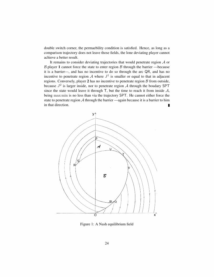
We need also consider the tertiary trajectory tangent to the barrier. This hap-pens at a point Q at t2 − t = π/4. A simple calculation shows that its parameter,the abscissa s2 of its end point in the primary field, is larger than s1. It reaches thesecondary field, at x = 1 at a point W. The corresponding secondary trajectoryintersects the barrier on its first arc, at a point R, while the secondary trajectory

22

corresponding to s = s1 cuts the same arc at a point S.We need to name two closed region : Call A the curvilinear triangle STP, and

B the area inside the closed contour QRSTQ

5.3.2 Nash equilibrium strategies

We now define a specific strategy pair (O stands for the origin (0, 0))

• In the primary field deprived of the region between the arc PTQO and the yaxis, (u1, u2) = (1,−1),

• in the secondary field deprived of A ∪ B, and of the part of the primary fieddescribed above, (u1, u2) = (−1, 1),

• in the tertiary field in the (tiny) region between the arc QW and the barrierQO, (u1, u2) = (1, 1),

• in region A, play the purely competitive strategies to reach the arc PT inmaxu1 minu2 time,

• in the region B, play the cooperative strategies to reach the arc QR in min-imum time, —a complex strategy pair, with a cooperative barrier— player1 making sure that the state does not leave that region by another part, i.e.playing u1 = 1 on the arc RU and u1 = −1 on the arcs UV and V,Q.

Theorem 3 The above strategy pair is a Nash equilibrium. The equilibrium payoffare characterized by J1 = s1 in region A, J1 = s2 in region B, and given by theprimary, secondary and tertiary fields elsewhere.

Proof In region A, the control u2 = 1 insures that the state cannot cross eitherthe arc SP nor the arc SU, it ca therefore only leave it through the arc PT. Onthat arc, player 2 switches to u2 = −1 making it impossible for player 1 to crossit towards larger J1 = s. Hence player 1 has no incentive to deviate. Conversly,since our strategy pair yields the fastest path to any point in the primary field, andfrom their to termination for player 2, he does not have any incentive to deviateeither.

A similar argument holds in region B, reversing roles: player 1 insures that thestate cannot leave it through any other arc than QR, which yields a larger J1 thanin the other fields adjacent to B. But against u2 = 1, he has no means of reachinga secondary trajectory with larger s.

Finally, in the regular, primary, secondary and tertiary fields, the Value func-tions are piecewise C1 and satisfy the Isaacs-Case equations. Moreover, at the

23

double switch corner, the permaebility condition is satisfied. Hence, as long as acomparison trajectory does not leave those fields, the lone deviating player cannotachieve a better result.

It remains to consider deviating trajectories that would penetrate region A orB.player 1 cannot force the state to enter region B through the barrier —becauseit is a barrier—, and has no incentive to do so through the arc QR, and has noincentive to penetrate region A where J1 is smaller or equal to that in adjacentregions. Conversely, player 2 has no incentive to penetrate region B from outside,because J2 is larger inside, nor to penetrate region A through the boudary SPTsince the state would leave it through T, but the time to reach it from inside A,being max min is no less than via the trajectory SPT. He cannot either force thestate to penetrate regionA through the barrier —again because it is a barrier to himin that direction.

Figure 1: A Nash equilibrium field

24

5.3.3 Minimax time game within region A

For the sake of completeness, let us describe the minimax time strategy in regionA. Te arc PT will be traversed with u1 = −1 and u2 = (2x− y− 3)/(y− 1). Wemay easily check that u2 ∈ [−1, 1], yet, the left limit requires checking that S is“above” the straight line y + x = 2, which is true. Using a classical construction,we assume that this arc will be reached by trajectories (u1, u2) = (−1, 1), andwe find that the Value gradient upon reaching the arc PT is given by (λ µ) =((y − 1)2/(y − 3) 0). Thus λ > 0 and just before reaching PT, µ > 0, which isin agreement with our guess concerning the controls. The signs of these gradientcoordinates do not change within an arc of circle of π/2, hence the region A isfilled by this simple field.

5.3.4 Cooperative minimum time strategies within region B

We now turn to the cooperative minimum time strategies within B. The first thingto do is to check that R has an ordinate y > 3. We assume that the arc WRwill be traversed at maximum speed with (u1, u2) = (−1, 1), and reached bytrajectories with (u1, u2) = (−1,−1), at least in the region y ≤ 3. A classicalconstruction leads to the fact that there is such a trajectory arriving at y = 3 whichis a cooperative barrier. At y < 3, the final Value gradient is given by (λ µ) =(1/(y − 3) 0). Hence λ is negative, as well as µ just before reaching the finalarc, which is in agreement with our guess concerning the controls. But before atime π/2 before reaching this arc, λ is positive, hence u1 = 1. We therefore find aswitch line, and the sace “above” is filled by the field before the switch.

There remains to investigate what happens on the arc QW. Here, the fastestway to traverse it is with u1 = −1 and u2 = (3 − x − y)/(1 − y). Again, itis readily checked that indeed, u2 ∈ [−1, 1]. If the incoming field is still with(u1, u2) = (−1,−1) (as on the adjacent arc WR), then one finds for the Value gra-dient (λ µ) = (−1/(3− y) 0). Hence, as wished, λ < 0 and also µ just beforereaching the final arc. Thus this smoothly extends the situation on the adjacent arc.

5.3.5 Half barrier

If we replace the cost J1 = x(T ) by the discontinuous J1 = x(T ) if x(T ) < 1and J1 = 1 + x(T ) if x(T ) ≥ 1, the trajectory arriving at s = 1 becomes a halfbarrier. Nothing else is modified in the game. Anyyhow, because the payment ofplayer one is purely final, all equilibrium trajectories are non-permeable surfacesfor him.

25

Figure 2: With a competitive field in region A and cooperative in region B

5.4 Variant

A more elegant, but less interesting, variant is with slighly modified dynamics, asfollows:

x = y − 2 + u1 , u1 ∈ [−1, 1] ,y = −x + 2u2 , u2 ∈ [−1, 1] ,

the rest of the problem being as in the original example.The primary field is as in the main example, with (u1, u2) = (1,−1), but the

double switch happens on the manifold x = −1, with y = s + 3. The secondaryfield, with (u1, u2) = (−1, 1) suffices, we shall not need the tertiary field.

The barrier cannot be continued backward beyound its point V where y = 3,x =

√13 − 2. The primary trajectory through that point has a parameter x(T ) =

s = 2. It intersects the corner manifold at a point P : x = −1, y = 5. Thesecondary trajectory reaching that point originates at the origin O. Thus the region

26

A is now the region OPVO.The purely time-optimal competitive field within the region A now involves

a barrier and an equivocal line. Together with the primary and secondary fieldsoutside of A, it provides a pair of Nash equilibrium strategies.

5.5 Conclusion of the example

As a substitute for a true conclusion, consider the question

“Why should player 1 cooperate in region B” ?

The answer is

“why not ?”

We argue that this is an equilibrium strategy, because if player 1 does anything else,any how the state will leave B through R giving the same payoff to him. Of course,should player 2 deviate, he would loose (increase the time to termination).

Now, one can specify any strategy for player 1 inside that region, providedthat it forbids crossing the competitive barrier. Then player 1’s strategy that mini-mizes the time to reach R against that particular strategy of player two constitutesan equlibrium pair with it. An averse player 1 may even choose to play a zero-sum game against player 2 with time to reach R as the criterion, as we proposedfor region A. The only interest of the choice we make here is to display both acompetitive barrier and a cooperative one in the same game.

(Concerning region A, the choice we made of a maximin behaviour is a retali-ation strategy needed to remove an incentive by player 2 to play u2 = −1 on, andclose to, the arc SP.)

Of course, this only stresses the very high lack of uniqueness of the Nash equi-librium concept.

6 Conclusion

Managing biological systems requires to model them. We have seen that many newproblems have arisen in the process. We feel that the arguments in favor of a morethorough analysis of two-player two-pure-strategy games are strong, in view of themotivation provided by evolutionary game theory. Yet, the concept of evolutionarystability will have to be revisited for such games.

Actually, we have shown here more open problems than new results. Our feel-ing, though, is that these are not completly out of reach. This is a challenge togame theoretists and managers of biological systems alike.

27

References

[1] A. AKHMETZHANOV, P. BERNHARD, F. GROGNARD, AND

L. MAILLERET, Competition between foraging predators and a hidingpreys as a nonzero-sum differential game, in Gamenets 2009, Istanbul,Turkey, 2009.

[2] R. BELLMAN Dynamic Programming, Princeton University Press, 1957.

[3] P. BERNHARD, Linear Differential Games and the Isotropic Rocket, PhDthesis, Stanford University, 1970.

[4] , Conditions de raccordement pour les jeux diffeerentiels, in IFAC WorldCongress, Paris, 1972.

[5] , New results about corners in differential games including state cos-traints, in IFAC World Congress, Boston, 1975.

[6] , Singular surfaces in differential games, an introduction, in Differentialgames and Applications, P. Haggedorn, G. Olsder, and H. Knoboloch, eds.,vol. 3 of Lecture Notes in Information and Control Sciences, Springer Verlag,Berlin, 1977, pp. 1–33.

[7] , Ess, population games, replicator dynamics: dynamics and games ifnot dynamic games, in International Symposium on the theory and applica-tions of dynamic games, no. 13, 2008.

[8] P. BERNHARD AND F. HAMELIN, Two-by-two static, evolutionary, and dy-namic games, in From Semantics to Computer Science: Essays in Honor ofGilles Kahn, Y. Bertot, G. Huet, J.-J. Levy, and G. Plotkin, eds., CambridgeUniversity Press, 2008, pp. 452–474.

[9] P. BERNHARD AND A. J. SHAIJU, Evolutionary stable strategies and dynam-ics: Tutorial, example and open problems, in 5th ISDG Workshop, Segovia,Spain, September 21–24, 2005, G. Martin-Herran, , and G. Zaccour, eds.,2005.

[10] O. BOLZA, Lectures on the Calculus of Variations, Cicago University Press,1904. (Reprint: Dover, 1961)

[11] A. BRESSAN AND F.S. PRIULI, Infinite horizon noncooperative differentialgames, J. of Differential Equations 227 (2006), pp. 230–257.

28

[12] A. BRESSAN AND F.S. PRIULI, Small BV Solutions of Hyperbolic Noncoop-erative Differential Games, SIAM J. on Control and Optimization 43 (2004),pp. 194–215.

[13] C. CARATHODORY, Calculus of Variations and Partial Differential Equationsof the First Order, 1935. Reprint: Holden-Day 1967.

[14] P. CARDALIAGUET AND S. PLASKACZ, Existence and uniqueness of a Nashequilibrium feedback for a simple nonzero-sum differential game, Internat. J.Game Theory 32 (2003) pp. 33–71.

[15] J.H. CASE, Toward a theory of many player differential games, SIAM Jour-nal on Control and Optimization 7 (1969), pp. 179–197.

[16] F. COURCHAMP, M. LANGLAIS, AND G. SUGIHARA, Cats protecting birds:modelling the mesopredator release effect Journal of Animal Ecology 68(1999), pp. 282–292.

[17] J. ENGWERDA, L.Q. Dynamic Optimization and Differential games, Wiley,2005.

[18] M. FAN, Y. KUANG, AND Z. FENG, Cats protecting birds revisited, Bulletinof mathematical biology 67 (2005), pp. 1081–1106.

[19] F. HAMELIN AND P. BERNHARD, Uncoupling Isaacs equations in two-player nonzero-sum differential games. Conflict over parental care as an ex-ample, Automatica, 44 (2008), pp. 882–885.

[20] F. HAMELIN, P. BERNHARD, A. SHAIJU, AND E. WAJNBERG, Diet selec-tion as a differential foraging game, SIAM journal on Control and Optimiza-tion, 46 (2007), pp. 1539–1561.

[21] F. HAMELIN, P. BERNHARD, AND E. WAJNBERG, Superparasitism as adifferential game, Theoretical Population Biology, 72 (2007), pp. 366–378.

[22] J. HOFBAUER AND K. SIGMUND, Evolutionary Games and Population Dy-namics, Cambridge University Press, Cambridge, U.K., 1998.

[23] R. ISAACS Games of Pursuit, Rand Report, 1951

[24] R. ISAACS Differential Games, John Wiley and Sons, 1965.

[25] J. MAYNARD SMITH, Evolution and the Theory of Games, Cambridge Uni-versity Press, Cambridge, U.K., 1982.

29

[26] J. MAYNARD SMITH AND G. R. PRICE, The logic of animal conflict, Nature,246 (1973), pp. 15–18.

[27] F.S. PRIULI, Nash Equilibrium Solutions for Noncooperative Non-zero SumDifferential Games, 13th ISDG International Symposium, Wrocław, Poland,2008.

[28] L. SAMUELSON, Evolutionary Games and Equilibrium Selection, MIT Press,Cambridge, Massachusetts, USA, 1997.

[29] W. SANDHOLM, Population Games, M.I.T. Press, To appear.

[30] A. SHAIJU AND P. BERNHARD, Evolutionarily stable strategies: Two non-trivial examples and a theorem, in International Symposium on DynamicGames and Applications, no. 12, Sophia Antipolis, France, 2006.

[31] J. G. WARDROP, Some theoretical aspects of road traffic research, Proceed-ings of the Institution of Civil Engineers, (1952), pp. 325–378.

[32] J. WEIBULL, Evolutionary Game Theory, M.I.T. Press, Cambridge, U.S.A.,1995.

A Proofs of subsection 2.2.3

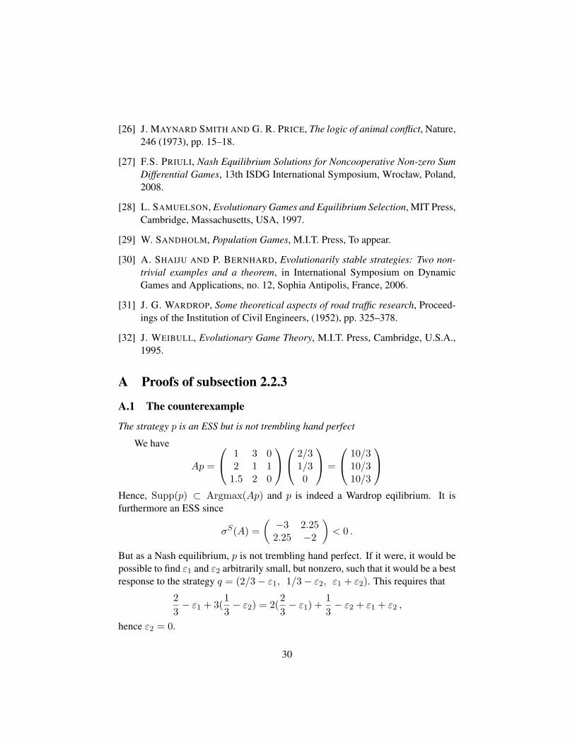
A.1 The counterexample

The strategy p is an ESS but is not trembling hand perfect

We have

Ap =

1 3 02 1 1

1.5 2 0

2/31/30

=

10/310/310/3

Hence, Supp(p) ⊂ Argmax(Ap) and p is indeed a Wardrop eqilibrium. It isfurthermore an ESS since

σS(A) =(

−3 2.252.25 −2

)< 0 .

But as a Nash equilibrium, p is not trembling hand perfect. If it were, it would bepossible to find ε1 and ε2 arbitrarily small, but nonzero, such that it would be a bestresponse to the strategy q = (2/3− ε1, 1/3− ε2, ε1 + ε2). This requires that

23− ε1 + 3(

13− ε2) = 2(

23− ε1) +

13− ε2 + ε1 + ε2 ,

hence ε2 = 0.

30

A.2 Proof of proposition 3

An ESS cannot weight positively a weakly dominated strategy

Assume to the contrary that the first trait is positively weighted by the ESS p,and weakly dominated by a trait not weighted by p, say trait m. The entries of linem in the game matrix A are thus larger or equal to the corresponding ones in line1.

The entries of line m in columns in Supp(p) are necessarily equal to the corrse-ponding ones in line 1, because if any was strictly larger, the m-th pure strategywould perform better, against p, than the first one, which itself performs as the ESSbecause of the equalization property. As a consequence, the coordinate m belongsto Argmax(Ap), and any strategy weighting the elements of Supp(p) and strategym is a best response to p.

Consider thus the strategy r which differs from p only in the fact that, on theone hand r1 = 0 and on the other hand rm = p1. It is a strategy, it belongs toBR(p). Now, against itself, it performs at least as well as p, in contradiction withthe strict inequality in condition (9).

If necessary, a simple way to check that statement is the following calculation.Consider the restrictions of the strategies and of the game matrix to Supp(p)∪{m}.Write

A =

a11 `1 a1m

c1 B cm

a11 `1 a1m

, p =

p1

p2

0

, r =

0p2

p1

.

Only keep in mind that p2 is —or may be— a (column) vector, `1 a line, and c1 andcm columns, all of the same dimension |Supp(p)| − 1. Also, B is a square matrixof the same dimension. With these notations, one easily obtains

〈p, Ar〉 = p1`1p2 + a1mp21 + 〈p2, Bp2〉+ 〈p2cm〉p1 ,

〈r, Ar〉 = 〈p2, Bp2〉+ 〈p2, cm〉p1 + p1`1p2 + ammp21 .

Hence F (r, r)− F (p, r) = (amm − a1m)p21 which is nonnegative if line m domi-

nates line 1.Assume now that p is mixed, and let {1 2} ⊂ Supp(p). And assume that line

2 dominates weakly line 1. As previously, the first two colomns of lines 1 and 2must coincide. Consider the strategy r obtained from p by transfering the weightof line 1, which is nonzero, on line 2. (Which is also what we have done, in fact,in the previous case.) It is in BR(p). But then, r − p = (−p1 p1 0 . . . 0), and as aconsequence 〈r − p, Ar〉 = 0, contradicting the second ESS condition.

31