Normal Vector Voting: Crease Detection and Curvature Estimation

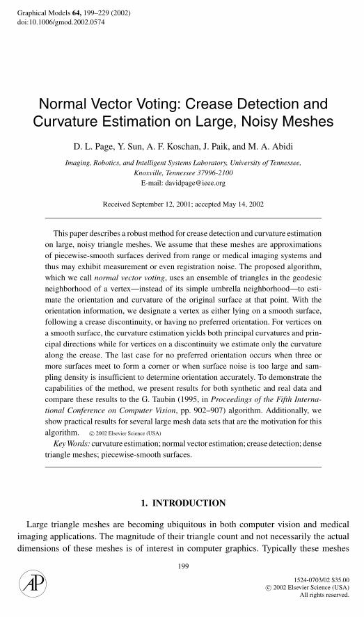
Graphical Models 64, 199–229 (2002)doi:10.1006/gmod.2002.0574

Normal Vector Voting: Crease Detection andCurvature Estimation on Large, Noisy Meshes

D. L. Page, Y. Sun, A. F. Koschan, J. Paik, and M. A. Abidi

Imaging, Robotics, and Intelligent Systems Laboratory, University of Tennessee,Knoxville, Tennessee 37996-2100

E-mail: [email protected]

Received September 12, 2001; accepted May 14, 2002

This paper describes a robust method for crease detection and curvature estimationon large, noisy triangle meshes. We assume that these meshes are approximationsof piecewise-smooth surfaces derived from range or medical imaging systems andthus may exhibit measurement or even registration noise. The proposed algorithm,which we call normal vector voting, uses an ensemble of triangles in the geodesicneighborhood of a vertex—instead of its simple umbrella neighborhood—to esti-mate the orientation and curvature of the original surface at that point. With theorientation information, we designate a vertex as either lying on a smooth surface,following a crease discontinuity, or having no preferred orientation. For vertices ona smooth surface, the curvature estimation yields both principal curvatures and prin-cipal directions while for vertices on a discontinuity we estimate only the curvaturealong the crease. The last case for no preferred orientation occurs when three ormore surfaces meet to form a corner or when surface noise is too large and sam-pling density is insufficient to determine orientation accurately. To demonstrate thecapabilities of the method, we present results for both synthetic and real data andcompare these results to the G. Taubin (1995, in Proceedings of the Fifth Interna-tional Conference on Computer Vision, pp. 902–907) algorithm. Additionally, weshow practical results for several large mesh data sets that are the motivation for thisalgorithm. c© 2002 Elsevier Science (USA)

Key Words: curvature estimation; normal vector estimation; crease detection; densetriangle meshes; piecewise-smooth surfaces.

1. INTRODUCTION

Large triangle meshes are becoming ubiquitous in both computer vision and medicalimaging applications. The magnitude of their triangle count and not necessarily the actualdimensions of these meshes is of interest in computer graphics. Typically these meshes

199

1524-0703/02 $35.00c© 2002 Elsevier Science (USA)

All rights reserved.

200 PAGE ET AL.

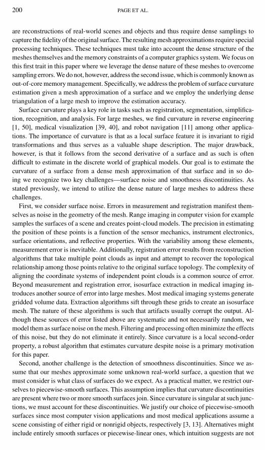
are reconstructions of real-world scenes and objects and thus require dense samplings tocapture the fidelity of the original surface. The resulting mesh approximations require specialprocessing techniques. These techniques must take into account the dense structure of themeshes themselves and the memory constraints of a computer graphics system. We focus onthis first trait in this paper where we leverage the dense nature of these meshes to overcomesampling errors. We do not, however, address the second issue, which is commonly known asout-of-core memory management. Specifically, we address the problem of surface curvatureestimation given a mesh approximation of a surface and we employ the underlying densetriangulation of a large mesh to improve the estimation accuracy.

Surface curvature plays a key role in tasks such as registration, segmentation, simplifica-tion, recognition, and analysis. For large meshes, we find curvature in reverse engineering[1, 50], medical visualization [39, 40], and robot navigation [11] among other applica-tions. The importance of curvature is that as a local surface feature it is invariant to rigidtransformations and thus serves as a valuable shape description. The major drawback,however, is that it follows from the second derivative of a surface and as such is oftendifficult to estimate in the discrete world of graphical models. Our goal is to estimate thecurvature of a surface from a dense mesh approximation of that surface and in so do-ing we recognize two key challenges—surface noise and smoothness discontinuities. Asstated previously, we intend to utilize the dense nature of large meshes to address thesechallenges.

First, we consider surface noise. Errors in measurement and registration manifest them-selves as noise in the geometry of the mesh. Range imaging in computer vision for examplesamples the surfaces of a scene and creates point-cloud models. The precision in estimatingthe position of these points is a function of the sensor mechanics, instrument electronics,surface orientations, and reflective properties. With the variability among these elements,measurement error is inevitable. Additionally, registration error results from reconstructionalgorithms that take multiple point clouds as input and attempt to recover the topologicalrelationship among those points relative to the original surface topology. The complexity ofaligning the coordinate systems of independent point clouds is a common source of error.Beyond measurement and registration error, isosurface extraction in medical imaging in-troduces another source of error into large meshes. Most medical imaging systems generategridded volume data. Extraction algorithms sift through these grids to create an isosurfacemesh. The nature of these algorithms is such that artifacts usually corrupt the output. Al-though these sources of error listed above are systematic and not necessarily random, wemodel them as surface noise on the mesh. Filtering and processing often minimize the effectsof this noise, but they do not eliminate it entirely. Since curvature is a local second-orderproperty, a robust algorithm that estimates curvature despite noise is a primary motivationfor this paper.

Second, another challenge is the detection of smoothness discontinuities. Since we as-sume that our meshes approximate some unknown real-world surface, a question that wemust consider is what class of surfaces do we expect. As a practical matter, we restrict our-selves to piecewise-smooth surfaces. This assumption implies that curvature discontinuitiesare present where two or more smooth surfaces join. Since curvature is singular at such junc-tions, we must account for these discontinuities. We justify our choice of piecewise-smoothsurfaces since most computer vision applications and most medical applications assume ascene consisting of either rigid or nonrigid objects, respectively [3, 13]. Alternatives mightinclude entirely smooth surfaces or piecewise-linear ones, which intuition suggests are not

NORMAL VECTOR VOTING 201

practical models of real-world surfaces. Piecewise smooth is the most appropriate choicebut for curvature estimation requires careful consideration at creases.

In this paper, we propose an algorithm called normal vector voting that addresses bothof the above issues and robustly estimates curvature for large dense triangle meshes. Thispaper is an enhancement and extension of the original algorithm first presented in [33]. Thecontributions of normal vector voting are as follows:

• application of geodesic neighborhoods to improve curvature estimation on largedense meshes,

• robust classification of surface orientation to account for curvature singularities atcreases and corners, and

• robust estimation of principal directions and principal curvatures to overcome sur-face measurement noise.

One contribution of this paper is the application of geodesic operations to curvature estima-tion. The dense triangulations of large meshes from computer vision and medical imagingenable geodesic operations to overcome sampling noise and thus to improve the quality ofestimation. Another contribution is the crease detection scheme that allows the algorithmto designate a mesh vertex as either on a smooth surface, at a crease junction, or with nopreferred orientation. The advantage of this classification is the detection and avoidanceof curvature singularities. Finally, a third contribution is the robust estimation of both theprincipal directions and principal curvatures. Previous methods have demonstrated robustcomputation of the principal curvatures alone but not the directions [43] while others havedemonstrated the computation of both but not in a robust manner [44]. Normal vector votingbridges the gap.

In the following sections, we present the normal vector voting algorithm and demonstrateits capabilities with several results. We first however present a quick background intocurvature in Section 2 and follow with a statement of our problem in Section 3. Then webriefly survey and categorize previous research in Section 4. In Section 5, we then outlineTaubin’s [44] formulation of the discrete estimation problem for curvature. Using Section 5as a starting point, we next outline in Section 6 the details of our normal vector votingalgorithm. This discussion includes a description of the voting process and orientationclassification as well as the curvature estimation. Section 7 presents practical results fromthe algorithm for large mesh examples while Section 8 compares the performance of ouralgorithm to Taubin’s original one. Finally we conclude in Section 9.

2. BACKGROUND

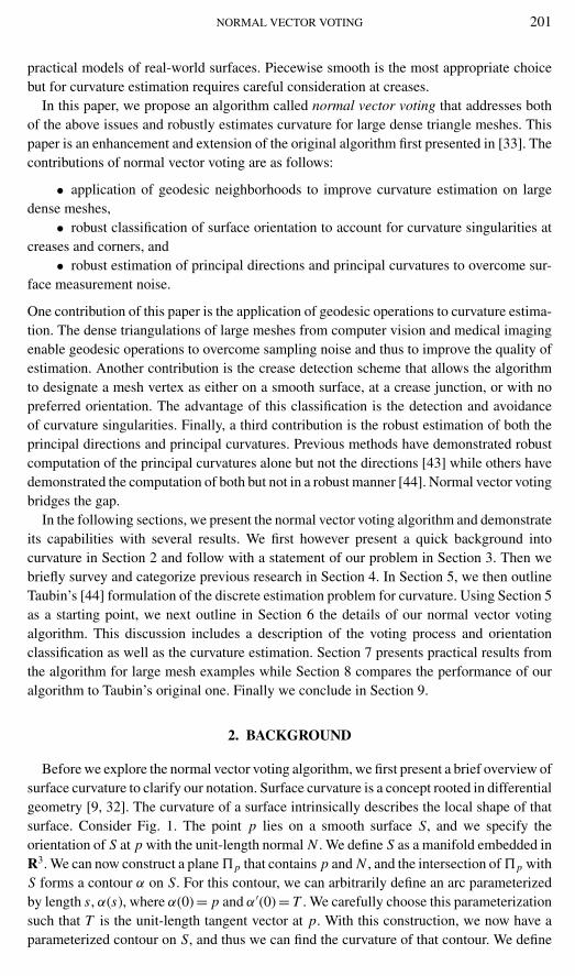
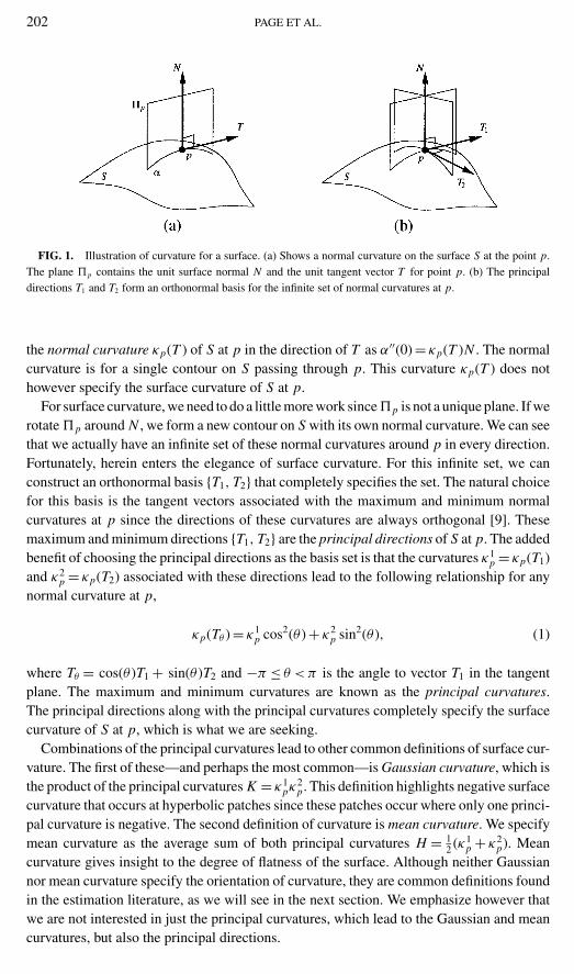
Before we explore the normal vector voting algorithm, we first present a brief overview ofsurface curvature to clarify our notation. Surface curvature is a concept rooted in differentialgeometry [9, 32]. The curvature of a surface intrinsically describes the local shape of thatsurface. Consider Fig. 1. The point p lies on a smooth surface S, and we specify theorientation of S at p with the unit-length normal N . We define S as a manifold embedded inR3. We can now construct a plane �p that contains p and N , and the intersection of �p withS forms a contour α on S. For this contour, we can arbitrarily define an arc parameterizedby length s, α(s), where α(0) = p and α′(0) = T . We carefully choose this parameterizationsuch that T is the unit-length tangent vector at p. With this construction, we now have aparameterized contour on S, and thus we can find the curvature of that contour. We define

202 PAGE ET AL.

FIG. 1. Illustration of curvature for a surface. (a) Shows a normal curvature on the surface S at the point p.The plane �p contains the unit surface normal N and the unit tangent vector T for point p. (b) The principaldirections T1 and T2 form an orthonormal basis for the infinite set of normal curvatures at p.

the normal curvature κp(T ) of S at p in the direction of T as α′′(0) = κp(T )N . The normalcurvature is for a single contour on S passing through p. This curvature κp(T ) does nothowever specify the surface curvature of S at p.

For surface curvature, we need to do a little more work since �p is not a unique plane. If werotate �p around N , we form a new contour on S with its own normal curvature. We can seethat we actually have an infinite set of these normal curvatures around p in every direction.Fortunately, herein enters the elegance of surface curvature. For this infinite set, we canconstruct an orthonormal basis {T1, T2} that completely specifies the set. The natural choicefor this basis is the tangent vectors associated with the maximum and minimum normalcurvatures at p since the directions of these curvatures are always orthogonal [9]. Thesemaximum and minimum directions {T1, T2} are the principal directions of S at p. The addedbenefit of choosing the principal directions as the basis set is that the curvatures κ1

p = κp(T1)and κ2

p = κp(T2) associated with these directions lead to the following relationship for anynormal curvature at p,

κp(Tθ ) = κ1p cos2(θ ) + κ2

p sin2(θ ), (1)

where Tθ = cos(θ )T1 + sin(θ )T2 and −π ≤ θ < π is the angle to vector T1 in the tangentplane. The maximum and minimum curvatures are known as the principal curvatures.The principal directions along with the principal curvatures completely specify the surfacecurvature of S at p, which is what we are seeking.

Combinations of the principal curvatures lead to other common definitions of surface cur-vature. The first of these—and perhaps the most common—is Gaussian curvature, which isthe product of the principal curvatures K = κ1

pκ2p. This definition highlights negative surface

curvature that occurs at hyperbolic patches since these patches occur where only one princi-pal curvature is negative. The second definition of curvature is mean curvature. We specifymean curvature as the average sum of both principal curvatures H = 1

2 (κ1p + κ2

p). Meancurvature gives insight to the degree of flatness of the surface. Although neither Gaussiannor mean curvature specify the orientation of curvature, they are common definitions foundin the estimation literature, as we will see in the next section. We emphasize however thatwe are not interested in just the principal curvatures, which lead to the Gaussian and meancurvatures, but also the principal directions.


Our challenge in estimating curvature is unfortunately that we are not dealing with acompletely smooth surface such as S above but rather a piecewise-smooth surface S wherewe apply the definition of a piecewise-smooth surface as in [2]. The surface S may forexample be the union of three smooth surfaces Sj , Sk , and Sl , manifolds embedded in R3,such that S = Sj ∪ Sk ∪ Sl . We assume that Sj , Sk , and Sl are orientable manifold surfaces,possibly with piecewise-smooth boundaries [2, 22], and that their subsequent union S alsoconforms to this same definition of a surface. Although this assumption may seem obvious,we explicitly state it for clarity. The subsequent piecewise-smooth surface has discontinuitycontours C jk = Sj ∩ Sk where two smooth surfaces join. The principal curvatures acrossthese contours are singular while their orthogonal counterparts, i.e., the principal curvaturesalong the contours, are not. Other discontinuities occur at corner points c jkl = Sj ∩ Sk ∩ Sl

where three or more surfaces join. Both principal curvatures are singular for such corners.Another challenge is that we are not actually working with S but rather with the mesh M

that approximates S. We specify M as the pair M = (K , V ) where K defines the topologyand V defines the geometry. We assume as with S that M is an orientable triangulatedmanifold surface, possibly with boundary [22]. The vertices V are samples of S such thatnoise may corrupt these samples. We have the following

v = p + e, (2)

where v ∈ V is a specific vertex of M, p ∈ S is a sample point on S, and e is a noise vectorthat accounts for measurement, registration, and isosurface extraction error. We can thinkof V as a point cloud and K as the interconnection of V to form the edges and faces of thetriangles in M .

3. PROBLEM STATEMENT

With the above background, we can now state our objective. The following statementsdefine the input and output of the normal vector voting algorithm.

Given a triangle mesh M = (K , V ) that approximates a piecewise-smooth surface S withcrease discontinuities C jk and corner points c jkl .

Estimate the principal curvatures κ1v and κ2

v and corresponding principal directions T1 andT2 for each vertex v ∈ V , which is a sample of p ∈ S.

The difficulty for this problem is that we must account for the singularities along the creasesp ∈ C jk and at corners p = c jkl and not allow these singularities to affect the estimation ofother samples near them. We must also account for the noise e that corrupts each sample.In the next section, we briefly review previous research into this problem.

4. PREVIOUS WORK

We have identified robust curvature estimation as a weakness in the current literature withregard to triangle meshes. In particular, we have not found a method that robustly estimatesboth principal curvatures and principal directions. Our proposed research intends to addressthis issue. Most research in the literature addresses curvature estimation in the context ofrange images with little work available for the more general problem of surface meshes.Since image processing and mesh processing require different tools, we do not intend to

204 PAGE ET AL.

address the direct estimation of curvature from range images. Our interest instead is toaddress the more general problem of curvature for a mesh data set. From our perspective wecan readily convert a range image into a triangle mesh, but to convert a mesh into a set ofrange images is not trivial and probably counterproductive. We refer the interested readerto [13] and [41] for excellent surveys into curvature-from-range methods.

Our review of the research literature reveals that only a few papers address the issue ofcurvature estimation on triangle meshes. Of those papers we have identified three classesof techniques:

• Surface fitting methods (SFMs),• Total curvature methods (TCMs), and• Curve fitting methods (CFMs).

We discuss each class briefly with special emphasis on the curve fitting methods as thoseoffer the most promise.

SFMs fit an analytic surface to the data of interest and then use differential geometry tocompute curvature from that function. With some modifications, we can use many of theanalytic methods for range images listed in [13] and [41]. We must construct however alocal parameterization of the surface similar to the parameterization that an image providesfor range data. The approaches of [18] and [38] provide possible choices for this parame-terization. Also Rossl et al. [38] use thresholds and morphological operations on a mesh toidentify smoothness discontinuities after estimation of curvature. Once we have a local pa-rameterization, we can use methods such as linear regression [10, 12, 39] or splines [31, 47]to estimate curvature. A more recent paper [37] uses a local fit of a biquadratic polynomialand applies smoothing to improve the analytic estimate of curvature.

TCMs are another class of algorithms. These algorithms use the topology and geometry ofthe mesh directly to estimate curvature. Total curvature—to be precise—is an integration oflocal curvature [32], and as such this class name may be misleading. Our intent in choosingthis nomenclature is to denote that these methods estimate curvature for a region and notjust at a single point. The other methods such as SFMs may use a region in their algorithmsbut their output is for a specific point on the mesh.

Since a triangle mesh is a piecewise-flat surface, the local curvature of such a surface isseemingly paradoxical [30]. The curvature is singular at each point on the surface—infiniteat vertices and edges and zero on triangle faces. We can however refer to the total curvaturefor regions on these surfaces. Lin and Perry [23] use the angle excess around each vertex toestimate the total Gaussian curvature. Angle excess itself is well known with [30] providinga nice discussion in the context of computer graphics and the Gauss–Bonnett theorem. Wefind another application of angle excess in a series of papers [5, 6] by Delingette. He laysout a framework for a surface representation that he calls a simplex mesh that is a dualto a triangle mesh. He discusses the total mean and the total Gaussian curvature for thissurface representation and shows these formulations are directly related to angle excess fora triangle mesh. We find another angle excess approach in the discrete minimal surfaceand straightest geodesic work of Polthier and his coauthors [34, 35]. Following this lineof research, Desbrun et al. [7] define a curvature normal vector as a discrete definition ofmean curvature for triangle meshes. As with the angle excess methods, Desbrun et al. useinterior angles of triangles for their formulation. With a different approach, Gourley [17]presents a total pseudo-curvature based on the dispersion of face normals around a vertexwhile Mangan and Whitaker [26] refine this measure as the norm of a covariance matrix


for these face normals. This pseudo-curvature is proportional to the magnitude of Gaussiancurvature. A novel algorithm from Wu and Levine [49] is a physics-based approach wherethey simulate the distribution of charge density across a mesh. They relate this chargedistribution to surface curvature. This approach also yields a pseudo-curvature measurethat is monotonically increasing relative to Gaussian curvature.

We finally consider the CFMs. With these methods, we fit a family of curves individuallyaround a point and then use the ensemble to estimate curvature. Martin [27] proposes amethod that selects vertex triples from a mesh and fits circles to those triples. Tookey andBall [45] describe a more sophisticated method that uses five points instead of three but isonly valid for data on a regular grid. Varady and Hermann [46] present an algorithm forcomputing principal curvature from a collection of surface curves using a linear system.A very interesting paper by Tang and Medioni [43] proposes a novel approach to infer thesign of Gaussian curvature and compute principal directions from noisy data. This methodis an evolution of Medioni’s tensor voting theory [28], which uses circular curves to discernfeatures from a point cloud. From the Duplin indicatrix, Chen and Schmitt [4] formulate aquadratic representation of curvature at each vertex and then derive the principal curvaturesusing a least squares minimization of the resulting overdetermined system. Inspired by thisapproach, Taubin [44] developed an algorithm that defines a symmetric matrix that has thesame eigenvectors as the principal directions and eigenvalues that are related by a fixedhomogeneous linear transformation to the principal curvatures. He estimates this matrix indiscrete form for a triangle mesh using vertex pairs that share a common edge. In the contextof surface reconstruction, Gopi et al. [16] extend Taubin’s algorithm beyond adjacent vertexpairs to arbitrarily close pairs and use a different weighting scheme. We finally note thecurvature work in the context of mesh simplification in Heckbert and Garland [19]. Thispaper outlines the relationship of the quadric error metric [14, 24] for triangle normals tocurvature.

The SFMs require the most computational effort since they typically employ optimizationin the fitting process. This optimization does provide some robustness to noise but does notinherently deal with discontinuities. The TCMs on the other hand are more computationallyefficient but are more susceptible to noise errors. The exception is the method of Wu andLevine [49] that does demonstrate robust results. None of the TCMs, however, directlyestimate the principal directions or principal curvatures that we seek. The CFMs are themost promising of the three classes. In particular, Tang and Medioni [43] and Taubin [44]offer unique contributions. Tang and Medioni’s method is robust but their algorithm doesnot estimate principal curvatures, only principal directions. They construct a matrix—similar to Taubin—whose eigenvectors relate to the principal directions but they do notshow how the eigenvalues relate to the principal curvatures. As stated above Taubin’salgorithm does. Taubin relates the eigenvalues to the principal curvatures. Our contributionis to extend both Tang and Medioni’s and Taubin’s methods with a new algorithm thatemploys a geodesic neighborhood, a voting scheme, and Taubin’s discrete formulation togenerate robust results. Before we present this novel approach, we next review Taubin’sformulation.

5. DISCRETE ESTIMATION

Our final preliminary step is to introduce the discrete formulation of curvature in accor-dance with Taubin [44]. Taubin shows that for a point p on a smooth surface the symmetric

206 PAGE ET AL.

matrix

Bp = 1

2π

∫ π

−π

κp(Tθ )Tθ T tθ dθ, (3)

with superscript t denoting transpose and Tθ as defined in Section 2, has eigenvectors thatare equivalent to the principal directions {T1, T2} and eigenvalues that are related by a fixedhomogeneous linear transformation to the principal curvatures as

κ1p = 3b1

p − b2p

(4)κ2

p = 3b2p − b1

p,

where b1p and b2

p are the eigenvalues of Bp associated with T1 and T2, respectively. The thirdeigenvalue is zero and corresponds to the eigenvector equal to the surface normal at p. Fora vertex v on a discrete mesh, Taubin approximates Eq. (3) as

Bv = 1

2π

∑wiκi Ti T

ti (5)

for a finite set of directions Ti in the tangent plane of v. The weight wi is the discreteintegration step and has the constraint

∑wi = 2π . Taubin’s algorithm computes Bv for a

vertex on a mesh and then decomposes the matrix with a Householder transformation and aGivens rotation. The resulting eigenvectors and eigenvalues lead to the principal directionsand principal curvatures via Eq. (4).

The question at hand is how do we estimate κi and Ti in Eq. (5). Taubin employs atruncated Laurent series to approximate these values, but this approach is not robust. Tangand Medioni [43] suggest a more robust solution. Building on these algorithms, we havedeveloped our normal vector voting algorithm as a robust method to estimate the individualκi and Ti and thus the principal directions and principal curvatures for a vertex on a mesh.We now take an in-depth look at this algorithm.

6. NORMAL VECTOR VOTING ALGORITHM

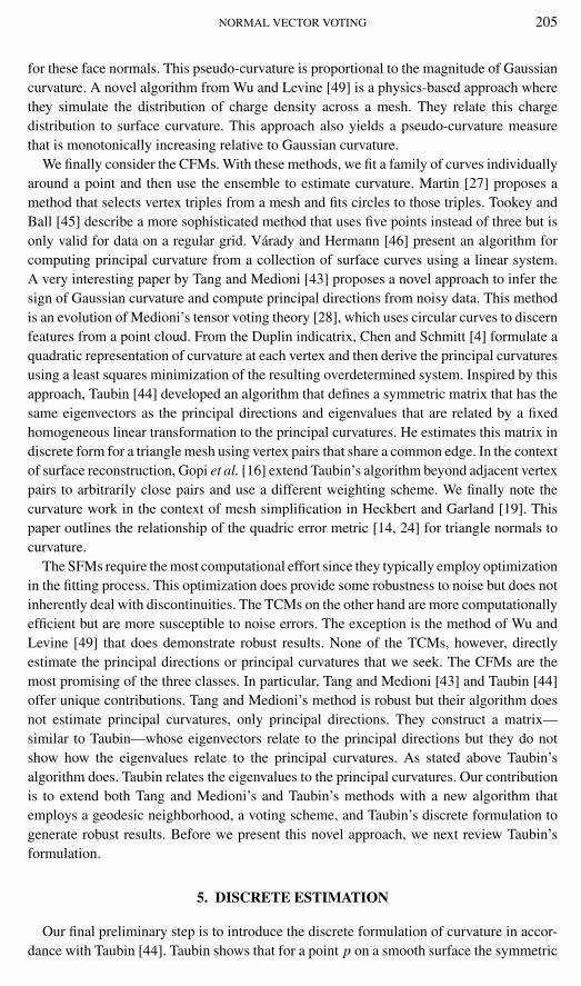
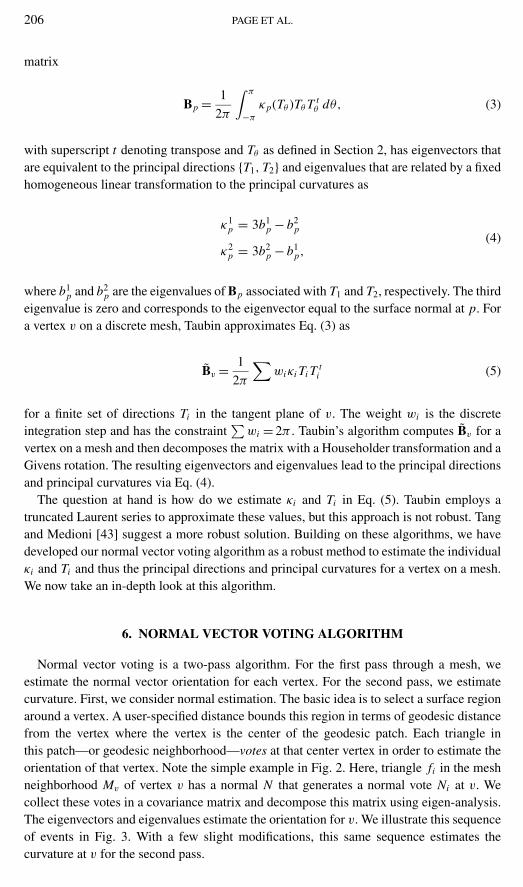
Normal vector voting is a two-pass algorithm. For the first pass through a mesh, weestimate the normal vector orientation for each vertex. For the second pass, we estimatecurvature. First, we consider normal estimation. The basic idea is to select a surface regionaround a vertex. A user-specified distance bounds this region in terms of geodesic distancefrom the vertex where the vertex is the center of the geodesic patch. Each triangle inthis patch—or geodesic neighborhood—votes at that center vertex in order to estimate theorientation of that vertex. Note the simple example in Fig. 2. Here, triangle fi in the meshneighborhood Mv of vertex v has a normal N that generates a normal vote Ni at v. Wecollect these votes in a covariance matrix and decompose this matrix using eigen-analysis.The eigenvectors and eigenvalues estimate the orientation for v. We illustrate this sequenceof events in Fig. 3. With a few slight modifications, this same sequence estimates thecurvature at v for the second pass.


FIG. 2. A triangle with normal N generates vote Ni for the orientation of the surface at v. The circular arcfollows the perceptual continuity constraints.

6.1. Geodesic Neighborhood

The first step in normal vector voting for both the first or the second pass is to find thetriangles or vertices that are close in a geodesic sense to the vertex of interest. The geodesicneighborhood problem, which follows the discrete geodesic problem [29], is to find the mtriangles that are within a user-specified distance of the vertex. The key is that the distance isnot the Euclidean distance but rather the shortest geodesic distance along the surface of themesh. As noted in the literature this problem closely resembles the shortest path problemfor a graph, which the Dijkstra algorithm [8] solves. The difference is that the shortest pathalong the edges and nodes of a graph is not necessarily equivalent to the shortest geodesicpath over the surface, which includes the triangle interiors and not just the edges. Kimmeland Sethian [21] present an elegant algorithm that solves this problem in O(m log m) timeand Sun and Abidi [42] propose a simplification that is readily adaptable to our domain.The time complexity is important when compared to such Euclidean algorithms as k-d treesthat require O(m + 3n2/3) time where n is the number of triangles in the whole mesh [48].Also, k-d trees require additional O(n) storage space beyond the current space required forthe mesh itself. The Kimmel and Sethian algorithm requires no additional storage.

As a brief aside, we distinguish the Kimmel and Sethian definition of shortest geodesicsfrom the straightest geodesics of Polthier and Schmies [35, 36]. The latter ensures theuniqueness of a geodesic path on a polyhedral surface. Since we are only concerned witha neighborhood and not the actual path, this trait is not crucial to our problem. We areinterested in shortest and not straightest geodesics.

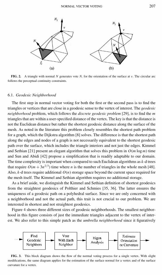
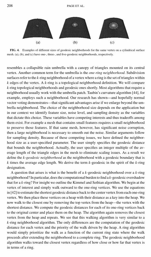
Figure 4 shows three different sizes of geodesic neighborhoods. The smallest neighbor-hood in this figure consists of just the immediate triangles adjacent to the vertex of inter-est. We also refer to this simple patch as the umbrella neighborhood since it figuratively

FIG. 3. This block diagram shows the flow of the normal voting process for a single vertex. With slightmodifications, the same diagram applies for the estimation of the surface normal for a vertex and of the surfacecurvature for a vertex.

208 PAGE ET AL.

FIG. 4. Examples of different sizes of geodesic neighborhoods for the same vertex on a cylindrical surfacemesh. (a), (b), and (c) have one-, three-, and five-geodesic neighborhoods, respectively.

resembles a collapsible rain umbrella with a canopy of triangles mounted on its centralvertex. Another common term for the umbrella is the one-ring neighborhood. Subdivisionsurfaces refer to the k-ring neighborhood of a vertex where a ring is the set of triangles withink edges of the vertex. A k-ring is a topological neighborhood definition. We will comparek-ring topological neighborhoods and geodesic ones shortly. Most algorithms that require aneighborhood usually work with the umbrella patch. Taubin’s curvature algorithm [44], forexample, employs such a neighborhood. Our research has shown—and hopefully normalvector voting demonstrates—that significant advantages arise if we enlarge beyond the um-brella neighborhood. The choice of the neighborhood size depends on the application butin our context we identify feature size, noise level, and sampling density as the variablesthat dictate this choice. These variables have competing interests and thus tradeoffs amongthem exist. For example a mesh that contains small features requires a small neighborhoodto preserve those features. If that same mesh, however, has significant noise corruption,then a large neighborhood is necessary to smooth out the noise. Similar arguments followfor sampling density. Because of these competing issues, we have defined the neighbor-hood size as a user-specified parameter. The user simply specifies the geodesic distancethat bounds the neighborhood. Actually, the user specifies an integer multiple of the av-erage length of the triangle edges in the mesh to eliminate scaling issues. As a result wedefine the k-geodesic neighborhood as the neighborhood with a geodesic boundary that isk times the average edge length. We derive the term k-geodesic in the spirit of the k-ringdesignation.

A question that arises is what is the benefit of a k-geodesic neighborhood over a k-ringneighborhood? In particular, does the computational burden to find a k-geodesic overshadowthat for a k-ring? For insight we outline the Kimmel and Sethian algorithm. We begin at thevertex of interest and simply walk outward to the one-ring vertices. We use the equationsin [42] to estimate the shortest geodesic distance back to the center vertex from each one-ringvertex. We then place these vertices on a heap with their distance as a key into the heap. Wenow walk to the closest one by removing the top vertex from the heap—the vertex with theshortest distance. We compute the geodesic distances for each of its one-ring vertices backto the original center and place them on the heap. The algorithm again removes the closestvertex from the heap and repeats. We see that this walking algorithm is very similar to ak-ring neighborhood algorithm. The only differences are the computation of the geodesicdistance for each vertex and the priority of the walk driven by the heap. A ring algorithmwould simply prioritize the walk as a function of the current ring state where the walkproceeds after extending the neighborhood to a complete ring. The geodesic neighborhoodalgorithm walks toward the closest vertex regardless of how close or how far that vertex isin terms of a ring.


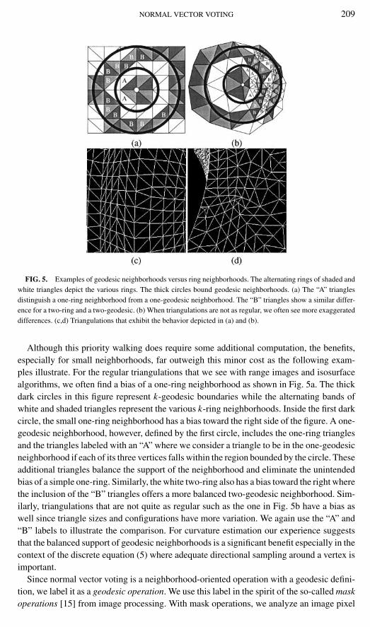
FIG. 5. Examples of geodesic neighborhoods versus ring neighborhoods. The alternating rings of shaded andwhite triangles depict the various rings. The thick circles bound geodesic neighborhoods. (a) The “A” trianglesdistinguish a one-ring neighborhood from a one-geodesic neighborhood. The “B” triangles show a similar differ-ence for a two-ring and a two-geodesic. (b) When triangulations are not as regular, we often see more exaggerateddifferences. (c,d) Triangulations that exhibit the behavior depicted in (a) and (b).

Although this priority walking does require some additional computation, the benefits,especially for small neighborhoods, far outweigh this minor cost as the following exam-ples illustrate. For the regular triangulations that we see with range images and isosurfacealgorithms, we often find a bias of a one-ring neighborhood as shown in Fig. 5a. The thickdark circles in this figure represent k-geodesic boundaries while the alternating bands ofwhite and shaded triangles represent the various k-ring neighborhoods. Inside the first darkcircle, the small one-ring neighborhood has a bias toward the right side of the figure. A one-geodesic neighborhood, however, defined by the first circle, includes the one-ring trianglesand the triangles labeled with an “A” where we consider a triangle to be in the one-geodesicneighborhood if each of its three vertices falls within the region bounded by the circle. Theseadditional triangles balance the support of the neighborhood and eliminate the unintendedbias of a simple one-ring. Similarly, the white two-ring also has a bias toward the right wherethe inclusion of the “B” triangles offers a more balanced two-geodesic neighborhood. Sim-ilarly, triangulations that are not quite as regular such as the one in Fig. 5b have a bias aswell since triangle sizes and configurations have more variation. We again use the “A” and“B” labels to illustrate the comparison. For curvature estimation our experience suggeststhat the balanced support of geodesic neighborhoods is a significant benefit especially in thecontext of the discrete equation (5) where adequate directional sampling around a vertex isimportant.

Since normal vector voting is a neighborhood-oriented operation with a geodesic defini-tion, we label it as a geodesic operation. We use this label in the spirit of the so-called maskoperations [15] from image processing. With mask operations, we analyze an image pixel

210 PAGE ET AL.

in terms of its own gray level and of the gray levels of its neighbors. We often specify themask neighborhood as k × k where k is the width in pixels of the mask centered at the pixelof interest. We see that our geodesic operation is similar except we specify the k-geodesicneighborhood of interest. We now have a geodesic neighborhood Mv . Our next step is tovote and determine the orientation of v or curvature at v depending on the pass.

6.2. Vote Collection

For the first pass, the next block in the diagram of Fig. 3 involves the voting of the trianglefaces fi ∈ Mv at the vertex v. We must address two questions:

• How does face fi cast a vote?• How does vertex v collect these votes?

To answer these questions, we are inspired by tensor voting in Medioni et al. [28]. Tensorvoting is a computational framework that infers structures such as boundaries and sur-faces from unstructured, sparse, and often noisy 3D point clouds. This framework employsperceptual constraints from theories of human vision and subsequent definitions of tensorvoting fields to extract structure. The implementation of tensor voting requires a discretevoxel representation of space where input points cast votes and voxels collect votes in thecontext of tensor algebra. Medioni et al. suggest a system of tensor voting fields in conjunc-tion with coordinate frame rotations and convolution-like operations with those fields toencode local geometric structure at each voxel. After the voting process, they extract salientglobal structures such as surfaces, curves, and junctions by sifting through these voxels witha level-crossing detection algorithm. Although the application of this approach to trianglemeshes is possible, we reformulate the tensor voting notions and propose a more naturalvector framework for triangle meshes. We use the same perceptual continuity constraintsas Medioni et al. to govern vote casting but we define a more appropriate vector geometryinstead of the tensor voting fields. For vote collection, we use a covariance matrix similarto the quadric error matrix in [19], which has a direct relationship to the tensor algebra inMedioni et al. Interestingly, Heckbert and Garland [19] show a relationship between thiscovariance matrix—in the limit—to surface curvature. We, however, use this matrix to es-timate orientation and later follow Taubin’s approach to estimate curvature. We have foundthat, in the presence of surface noise, this two-step approach is more robust than directlyextracting curvature from the covariance matrix.

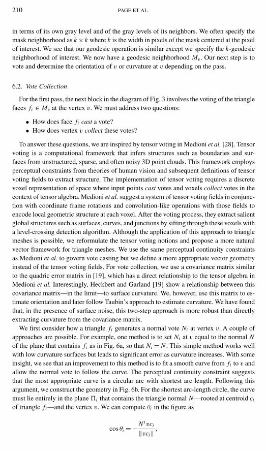
We first consider how a triangle fi generates a normal vote Ni at vertex v. A couple ofapproaches are possible. For example, one method is to set Ni at v equal to the normal Nof the plane that contains fi as in Fig. 6a, so that Ni = N . This simple method works wellwith low curvature surfaces but leads to significant error as curvature increases. With someinsight, we see that an improvement to this method is to fit a smooth curve from fi to v andallow the normal vote to follow the curve. The perceptual continuity constraint suggeststhat the most appropriate curve is a circular arc with shortest arc length. Following thisargument, we construct the geometry in Fig. 6b. For the shortest arc-length circle, the curvemust lie entirely in the plane �i that contains the triangle normal N—rooted at centroid ci

of triangle fi —and the vertex v. We can compute θi in the figure as

cos θi = − N tvci

‖vci‖ ,


FIG. 6. Geometries for normal vector voting. (a) A simple translation of N (Ni = N ). (b) A slightly moresophisticated vote where we rotate N by (2θi − π ) in plane �i . (c) Curvature estimation geometry where Nv , ni ,and Ti lie in the plane �i and ni is the projection of Nvi onto the plane.

where vci = ci − v and 0 ≤ θi ≤ π . This equation leads to the normal vote

Ni = N + 2 cos θivci

‖vci‖ . (6)

We next address how v collects the Ni votes from each fi ∈ Mv . One possibility is asa weighted vector sum

∑wi Ni . This approach is a common method for normal vector

estimation at vertices in a triangle mesh, typically with an umbrella neighborhood. Thelimitation of this scheme is that normals with opposite orientation annihilate each other(N j = −Ni , N j + Ni = �0), and we therefore lose variance information. This situation occursnear crease and corner discontinuities in particular. As an alternative, we represent Ni as acovariance matrix Vi = Ni N t

i and collect votes as a weighted matrix sum Vv with

Vv =∑

wi Vi =∑

wi Ni N ti , (7)

where the summation is over the Mv neighborhood. Unfortunately, the downside is thatwe now lose absolute sign orientation. The covariance matrix Vi does not designate whichside of the mesh is the outside of the surface. Consider N j = −Ni . How do we distinguishNi N t

i = N j N tj ? The benefit is that these votes no longer annihilate each other. We can track

the variance of the votes. This capability outweighs the loss of the absolute sign informationsince the variance allows us to draw conclusions about the relative orientation of the vertex.We will see in a later section that eigen-analysis of this variance leads to an interestingclassification scheme for the vertex. With regard to the absolute sign, we should be able torecover this information with a simple ad hoc algorithm such as a quick averaging of theumbrella neighbors. Only under a pathological case does such an approach fail. So we canreadily overcome the sign problem.

Our final issue to address is the weighting term wi . Two factors effect this term: surfacearea of fi and geodesic distance gi of ci from v. Naturally, a triangle closer to v should havea stronger vote than a triangle farther away while a larger one should also have a strongervote than a smaller one. We choose an exponential decay to reflect these notions

wi = Ai

Amaxexp

(−gi

σ

), (8)

where σ controls the rate of decay, Ai is the area of fi , and Amax is the area of the largest

212 PAGE ET AL.

triangle in the entire mesh. In practice, the value σ is a function of the maximum geodesicdistance that the user specifies. We define this value to be 3σ = gm so that votes beyond theneighborhood have negligible influence and can be ignored.

The above equations lead to a covariance matrix Vv for each vertex v in the mesh. Thismatrix represents the variance of the votes in the geodesic neighborhood Mv around v. Inthe next section, we use eigen-analysis to investigate the orientation of v using this varianceinformation.

6.3. Orientation Classification

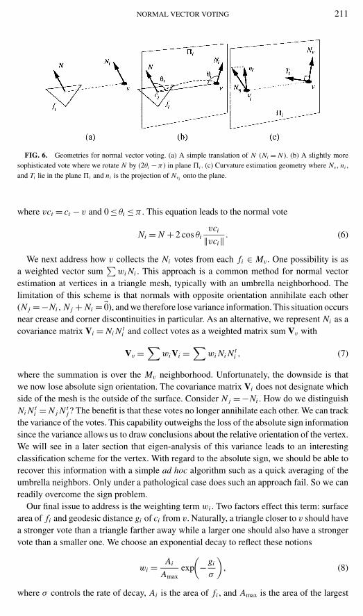
While still in the first pass of the algorithm, the third step in Fig. 3 is to decomposeVv using eigen-analysis and then to classify v. Since Vv is a symmetric semidefinite ma-trix, eigen-decomposition generates real eigenvalues λ1 ≥ λ2 ≥ λ3 ≥ 0 with correspondingeigenvectors E1, E2, and E3. We can visualize this eigensystem as in Fig. 7a. The eigenval-ues, and thus the shape of the eigen-ellipsoid, yield insight into the vote agreement withinVv . Figures 7b–7d show three variations of the eigenvalues and how we might interpretthese variations.

In tensor voting, Medioni et al. [28] define saliency maps over the entire voxel spacewith eigenvalues from their tensors. They then use an extremal search algorithm to extractsalient global structures from these map definitions. The saliency maps use the followingrelationships for their tensor eigenvalues:

Ss = λ1 − λ2, surface patch saliency;

Sc = λ2 − λ3, crease junction saliency; and

Sn = λ3, no preferred orientation saliency.

(9)

Since we seek to classify the preferred orientation of a vertex as opposed to the globalstructure through a voxel, we take a different approach and do not employ a search algorithmto sort through voxels. For our vector voting, we propose the following vertex classification

FIG. 7. These ellipsoids depict possible variations in the eigenvalues. We interpret these variations of Vv asthe orientation saliency of the neighborhood around v. (a) Covariance matrix Vv where the eigenvalues λ1, λ2,and λ3 define the shape. (b) Surface patch where λ1 is much larger than λ2, and λ3. (c) Crease discontinuity whereλ1, and λ2 are similar in value but larger than λ3. (d) Patch with no preferred orientation where each eigenvalue issimilar in value.


scheme for the eigenvalues of Vv at each vertex:

max{Ss, εSc, εηSn} =

Ss : surface patch with normal Nv = E1

εSc: crease junction with tangent Tv = E3

εηSn: no preferred orientation

(10)

where 0 ≤ ε < ∞ and 0 ≤ η < ∞ are constants that control the relative significance of thesaliency measures. These constants are not user parameters since they are fixed for a givensystem. When we design a system, however, we need to carefully select these constants tobalance noise tolerance and crease detection.

We demonstrate the design impact of ε and η with examples. First, consider one ex-treme where we design ε = η = 0. This system always classifies a vertex as a surface patchregardless of any corners or creases in the original piecewise-smooth surface. Consider

limε,η→0

max{Ss, εSc, εηSn} =Ss .

This design associates a surface normal with each vertex even if the vertex is a sample of acrease or a corner. Thus, the design does not detect curvature discontinuities. This approachis very similar to a normal estimation algorithm that averages the triangle normals of a one-ring neighborhood for a vertex. Another design extreme lets ε, η → ∞. Such a system neverclassifies a vertex as a surface patch regardless of smoothness and instead classifies eachvertex as a corner. This design never assigns surface normals to vertices. The third extremeis a design where ε → ∞ and η = 0. As we might expect, this system always classifies avertex as a crease and associates a tangent vector with the vertex. Although the first designmay have some use, the latter two designs have little practical use, but they do illustratethe choice of the constants (ε, η). When designing a system, we fix ε to discriminate thetypes of creases that we expect in the piecewise-smooth surfaces and η to discriminate theamount of surface noise that we wish to tolerate in our sensors.

For a system design, we need to decide how much noise we can tolerate and what creaseangles we need to detect. If we choose to detect small creases, we reduce the overallrobustness of the system. On the other hand, less tolerance to small creases allows moretolerance to noise. The constant ε controls these design considerations. In our experiments,the system ε = 2 offers a balanced compromise of detecting creases and allowing variation.As a rule of thumb, we have the following equation

tanφ

2=

√1

ε + 1, (11)

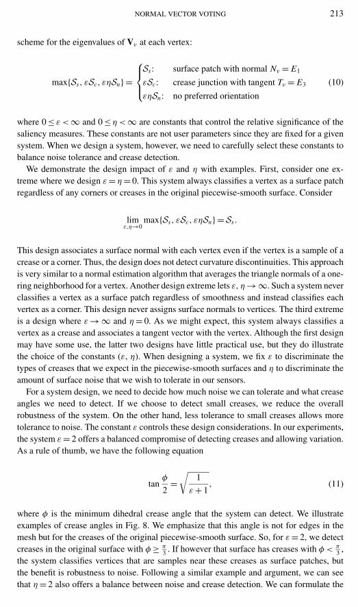
where φ is the minimum dihedral crease angle that the system can detect. We illustrateexamples of crease angles in Fig. 8. We emphasize that this angle is not for edges in themesh but for the creases of the original piecewise-smooth surface. So, for ε = 2, we detectcreases in the original surface with φ ≥ π

3 . If however that surface has creases with φ < π3 ,

the system classifies vertices that are samples near these creases as surface patches, butthe benefit is robustness to noise. Following a similar example and argument, we can seethat η = 2 also offers a balance between noise and crease detection. We can formulate the

214 PAGE ET AL.

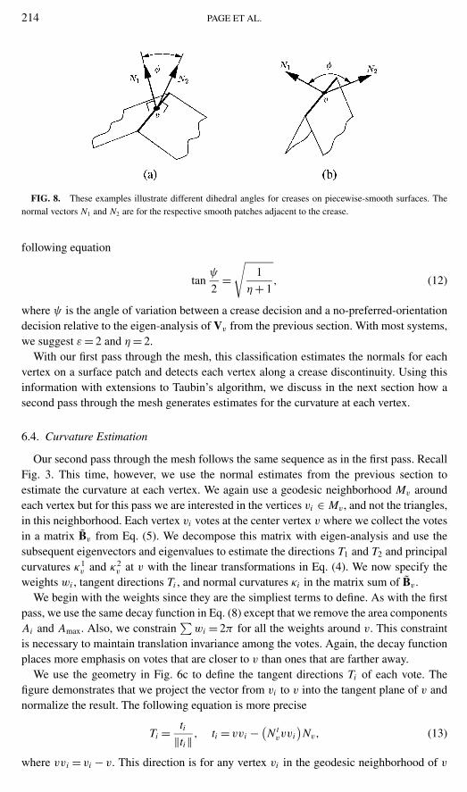
FIG. 8. These examples illustrate different dihedral angles for creases on piecewise-smooth surfaces. Thenormal vectors N1 and N2 are for the respective smooth patches adjacent to the crease.

following equation

tanψ

2=

√1

η + 1, (12)

where ψ is the angle of variation between a crease decision and a no-preferred-orientationdecision relative to the eigen-analysis of Vv from the previous section. With most systems,we suggest ε = 2 and η = 2.

With our first pass through the mesh, this classification estimates the normals for eachvertex on a surface patch and detects each vertex along a crease discontinuity. Using thisinformation with extensions to Taubin’s algorithm, we discuss in the next section how asecond pass through the mesh generates estimates for the curvature at each vertex.

6.4. Curvature Estimation

Our second pass through the mesh follows the same sequence as in the first pass. RecallFig. 3. This time, however, we use the normal estimates from the previous section toestimate the curvature at each vertex. We again use a geodesic neighborhood Mv aroundeach vertex but for this pass we are interested in the vertices vi ∈ Mv , and not the triangles,in this neighborhood. Each vertex vi votes at the center vertex v where we collect the votesin a matrix Bv from Eq. (5). We decompose this matrix with eigen-analysis and use thesubsequent eigenvectors and eigenvalues to estimate the directions T1 and T2 and principalcurvatures κ1

v and κ2v at v with the linear transformations in Eq. (4). We now specify the

weights wi , tangent directions Ti , and normal curvatures κi in the matrix sum of Bv .We begin with the weights since they are the simpliest terms to define. As with the first

pass, we use the same decay function in Eq. (8) except that we remove the area componentsAi and Amax. Also, we constrain

∑wi = 2π for all the weights around v. This constraint

is necessary to maintain translation invariance among the votes. Again, the decay functionplaces more emphasis on votes that are closer to v than ones that are farther away.

We use the geometry in Fig. 6c to define the tangent directions Ti of each vote. Thefigure demonstrates that we project the vector from vi to v into the tangent plane of v andnormalize the result. The following equation is more precise

Ti = ti‖ti‖ , ti = vvi − (

N tvvvi

)Nv, (13)

where vvi = vi − v. This direction is for any vertex vi in the geodesic neighborhood of v


and not just the umbrella neighbors as in Taubin’s algorithm. The normal Nv is the estimatefrom the previous section.

Last we consider the normal curvatures κi . We propose a discrete definition using thechanges in turning angle ϑi and in arc length s where

κi = �ϑi

�s. (14)

An important consideration is that we properly define the turning angle for the normal curveand not just the curve connecting vi and v. The change in the turning angle describes thechange in the normal vector as we move along the curve. To this end, we project the normalestimate Nvi at vi into the plane �i that contains Nv—rooted at v—and vi as

ni = Nvi − (Pt

i Nvi

)Pi , (15)

where ni is the projection and Pi = Nv × Ti defines the plane that contains the normal curve.The turning angle thus becomes

cos(�ϑi ) = N tvni

‖ni‖ . (16)

The sign of κi is the same as the sign of T ti ni . Finally, the change in arc length is simply

the geodesic distance between the two vertices

�s = gi . (17)

We estimate gi from the geodesic neighborhood algorithm discussed in Section 6.1. Fora vertex v, we collect the curvature votes from the equations above into the matrix Bv ofEq. (5), and eigen-decomposition leads to the principal directions T1 and T2 and principalcurvatures κ1

v and κ2v from the relation in Eq. (4).

6.5. Remarks

We have reached our goal. After the second pass, we have an estimate for the curva-ture at each vertex. We discuss a few caveats, however. First we only compute surfacecurvature if we classify a vertex as a surface patch. If a vertex has no preferred orientation,surface curvature is meaningless. A vertex on a crease on the other hand is a little differentsince we can estimate the curvature in the direction of the crease. With slight modificationsof the above equations, we can generate a tangential curvature estimate. The other principalcurvature, which is orthogonal to this one, is infinite, but we can estimate the cusp angle

across the crease as either φ = 2 arctan√

λ1λ2

or (π − 2φ) where λ1 and λ2 are the eigenvalues

from the first pass through the mesh in Section 6.3. The choice for the angle depends onthe absolute sign information that our ad hoc umbrella method resolves. We further notethat our classification scheme does not enforce crease continuity, i.e., topologically linkcrease vertices. If such topological connectivity is important, we suggest morphologicaloperations [38] or watershed methods [26]. The final caveat relates to the neighborhooddefinition. The neighborhood algorithm is a fast marching method that begins at the vertexof interest v as the center and marches out to form the neighborhood Mv . For curvatureestimation as the algorithm marches outward, we check the classification of the currentvertex and only proceed if it is a surface patch. This qualification does not allow the marching

216 PAGE ET AL.

algorithm to cross crease discontinuities and thus restricts Mv to the same smooth patchas v. This approach improves the curvature estimate since vertices on the other side of adiscontinuity do not corrupt the estimation.

7. EXPERIMENTAL RESULTS

We have implemented the proposed algorithm in C++ code. To demonstrate the algorithmcapabilities, we have experimented with a variety of data sets from CAD models to rangereconstructions to medical isosurfaces. In this section, we present the qualitative resultsof these experiments and follow in the next section with quantitative results from a morecontrolled experiment. In the discussions that follow, we designate the single user parameterof the normal vector voting algorithm gm as an integer multiple of the average edge length lave

for mesh triangles. So gm = 5lave means that we set the geodesic neighborhood boundary tofive times the average edge length. We alternatively use the term five-geodesic neighborhoodpresented in a previous section. When pertinent we also call out the system constants ε andη that we used for a particular design. These constants in practice are fixed and should notchange. Rather, we control the algorithm with the neighborhood boundary and not theseconstants.

We first consider two illustrative data sets: a fandisk in Fig. 9 and a torus in Fig. 10.The fandisk is a CAD model that exemplifies free-form smooth surfaces, and the torus is a

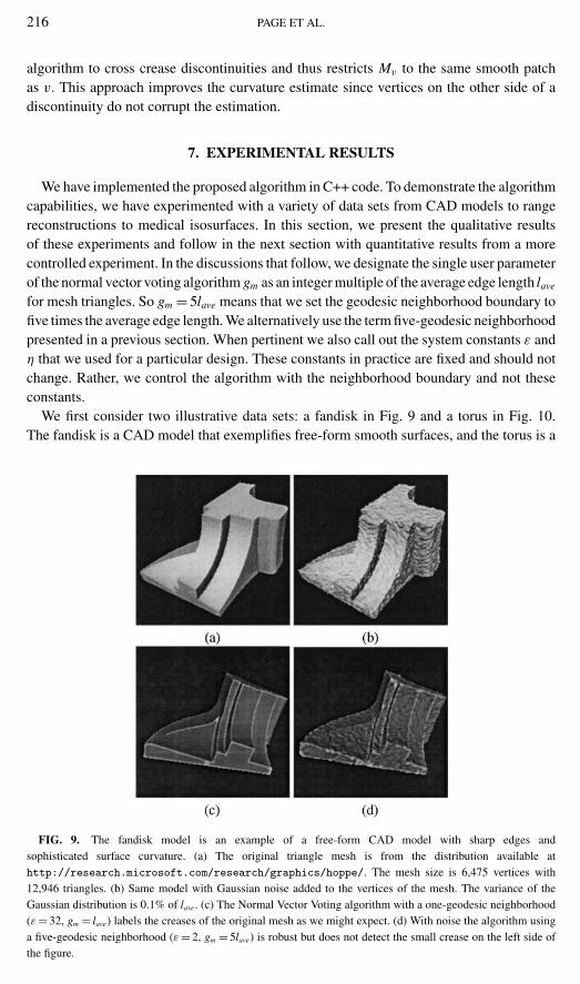
FIG. 9. The fandisk model is an example of a free-form CAD model with sharp edges andsophisticated surface curvature. (a) The original triangle mesh is from the distribution available athttp://research.microsoft.com/research/graphics/hoppe/. The mesh size is 6,475 vertices with12,946 triangles. (b) Same model with Gaussian noise added to the vertices of the mesh. The variance of theGaussian distribution is 0.1% of lave. (c) The Normal Vector Voting algorithm with a one-geodesic neighborhood(ε = 32, gm = lave) labels the creases of the original mesh as we might expect. (d) With noise the algorithm usinga five-geodesic neighborhood (ε = 2, gm = 5lave) is robust but does not detect the small crease on the left side ofthe figure.


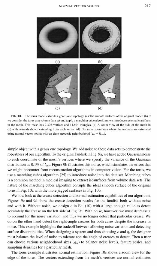
FIG. 10. The torus model exhibits a genus one topology. (a) The smooth surfaces of the original model. (b) Ifwe consider the torus as a volume data set and apply a marching cube algorithm, we introduce systematic artifactsin the mesh. This mesh has 7,302 vertices and 14,604 triangles. (c) A zoom view of the side of the mesh in(b) with normals shown extending from each vertex. (d) The same zoom area where the normals are estimatedusing normal vector voting with an eight-geodesic neighborhood (gm = 8lave).

simple object with a genus one topology. We add noise to these data sets to demonstrate therobustness of our algorithm. To the original fandisk in Fig. 9a, we have added Gaussian noiseto each coordinate of the mesh’s vertices where we specify the variance of the Gaussiandistribution as 0.1% of lave. Figure 9b illustrates this noise, which simulates the errors thatwe might encounter from reconstruction algorithms in computer vision. For the torus, weuse a marching cubes algorithm [25] to introduce noise into the data set. Marching cubesis a common method in medical imaging to extract isosurfaces from volume data sets. Thenature of the marching cubes algorithm corrupts the ideal smooth surface of the originaltorus in Fig. 10a with the more jagged surfaces in Fig. 10b.

We now look at the crease detection and normal estimation capabilities of our algorithm.Figures 9c and 9d show the crease detection results for the fandisk both without noiseand with it. Without noise, we design ε in Eq. (10) with a large enough value to detectaccurately the crease on the left side of Fig. 9c. With noise, however, we must decrease ε

to account for the noise variation, and thus we no longer detect that particular crease. Wedo on the other hand detect the right-angle creases for both cases despite the increase innoise. This example highlights the tradeoff between allowing noise variation and detectingsurface discontinuities. When designing a system and thus choosing ε and η, the designermust balance the level of noise to tolerate and the angle of creases to detect. Then a usercan choose various neighborhood sizes (gm) to balance noise levels, feature scales, andsampling densities for a particular mesh.

The torus example illustrates normal estimation. Figure 10c shows a zoom view for theedge of the torus. The vectors extending from the mesh’s vertices are normal estimates

218 PAGE ET AL.

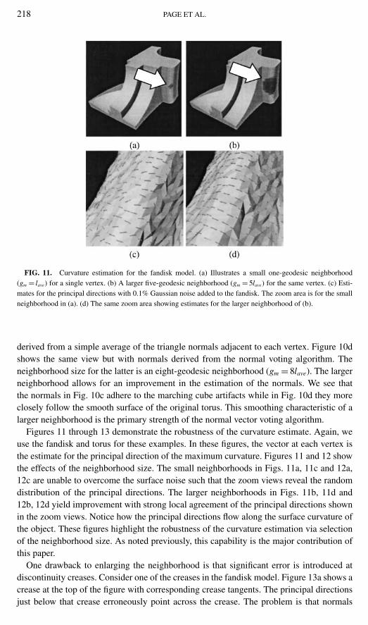
FIG. 11. Curvature estimation for the fandisk model. (a) Illustrates a small one-geodesic neighborhood(gm = lave) for a single vertex. (b) A larger five-geodesic neighborhood (gm = 5lave) for the same vertex. (c) Esti-mates for the principal directions with 0.1% Gaussian noise added to the fandisk. The zoom area is for the smallneighborhood in (a). (d) The same zoom area showing estimates for the larger neighborhood of (b).

derived from a simple average of the triangle normals adjacent to each vertex. Figure 10dshows the same view but with normals derived from the normal voting algorithm. Theneighborhood size for the latter is an eight-geodesic neighborhood (gm = 8lave). The largerneighborhood allows for an improvement in the estimation of the normals. We see thatthe normals in Fig. 10c adhere to the marching cube artifacts while in Fig. 10d they moreclosely follow the smooth surface of the original torus. This smoothing characteristic of alarger neighborhood is the primary strength of the normal vector voting algorithm.

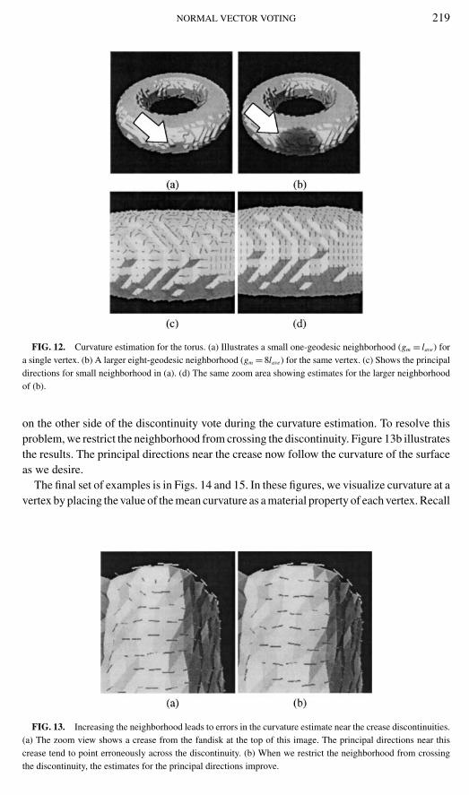
Figures 11 through 13 demonstrate the robustness of the curvature estimate. Again, weuse the fandisk and torus for these examples. In these figures, the vector at each vertex isthe estimate for the principal direction of the maximum curvature. Figures 11 and 12 showthe effects of the neighborhood size. The small neighborhoods in Figs. 11a, 11c and 12a,12c are unable to overcome the surface noise such that the zoom views reveal the randomdistribution of the principal directions. The larger neighborhoods in Figs. 11b, 11d and12b, 12d yield improvement with strong local agreement of the principal directions shownin the zoom views. Notice how the principal directions flow along the surface curvature ofthe object. These figures highlight the robustness of the curvature estimation via selectionof the neighborhood size. As noted previously, this capability is the major contribution ofthis paper.

One drawback to enlarging the neighborhood is that significant error is introduced atdiscontinuity creases. Consider one of the creases in the fandisk model. Figure 13a shows acrease at the top of the figure with corresponding crease tangents. The principal directionsjust below that crease erroneously point across the crease. The problem is that normals


FIG. 12. Curvature estimation for the torus. (a) Illustrates a small one-geodesic neighborhood (gm = lave) fora single vertex. (b) A larger eight-geodesic neighborhood (gm = 8lave) for the same vertex. (c) Shows the principaldirections for small neighborhood in (a). (d) The same zoom area showing estimates for the larger neighborhoodof (b).

on the other side of the discontinuity vote during the curvature estimation. To resolve thisproblem, we restrict the neighborhood from crossing the discontinuity. Figure 13b illustratesthe results. The principal directions near the crease now follow the curvature of the surfaceas we desire.

The final set of examples is in Figs. 14 and 15. In these figures, we visualize curvature at avertex by placing the value of the mean curvature as a material property of each vertex. Recall

FIG. 13. Increasing the neighborhood leads to errors in the curvature estimate near the crease discontinuities.(a) The zoom view shows a crease from the fandisk at the top of this image. The principal directions near thiscrease tend to point erroneously across the discontinuity. (b) When we restrict the neighborhood from crossingthe discontinuity, the estimates for the principal directions improve.

220 PAGE ET AL.


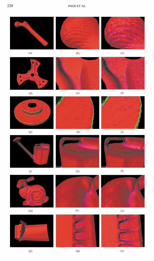
that the mean curvature is simply the average curvature of both principal curvatures. Thisvisualization allows us to investigate the relative accuracy between normal vector votingand Taubin’s algorithm. The zoom views demonstrate this comparison. Notice that themiddle column for normal vector voting exhibits a smoother variation in curvature despitethe surface noise for each data set while the right column for Taubin’s algorithm follows thenoise. The right column zooms are more splotchy than the middle ones, which is indicat-ive of noise. These figures and the previous ones give insight to the relative capabilities ofnormal vector voting, but in the next section, we explore a more quantitative analysis toidentify more clearly these capabilities.

8. COMPARISON RESULTS

The previous examples show the capabilities of the normal vector voting algorithm butdo not provide a baseline for comparison. Figures 16, 18, and 20 attempt to do so. In thesefigures, we graph the error of the algorithm for both synthetic and real data where we useground truth to establish the error. For these graphs, we manipulate three variables: surfacetype, noise level, and neighborhood size.

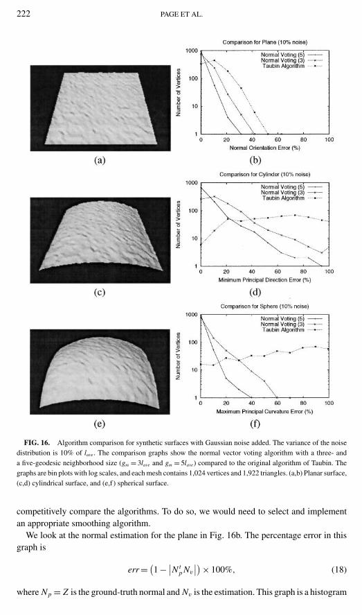
We first consider synthetic data to evaluate noise sensitivity. We choose three surfacetypes: planar, cylindrical, and spherical. The radius of curvature for the cylinder and thesphere is 31 mm. Figures 16a, 16c, and 16e show these surfaces with Gaussian noise addedto the Z coordinate using a distribution variance of 10% of lave. The graphs in Figs. 16b,16d, and 16f compare the performance of the normal vector voting algorithm for a three-and five-geodesic neighborhood (gm = 3lave and gm = 5lave) to Taubin’s one-ring algorithm.We have chosen to compare to Taubin’s algorithm since it serves as the foundation forour algorithm. We do not compare results for Tang and Medioni’s algorithm since theiralgorithm is for point-cloud data sets and since they do not compute principal directionsfor surface curvature.

Taubin’s algorithm serves to baseline the performance of our method. However, fornoisy surfaces, a direct comparison is perhaps not appropriate since—as Taubin notes—his algorithm requires a smoothing step to preprocess any surface noise. In fairness toTaubin, we emphasize that we baseline the benefits of the k-geodesic neighbors and do not

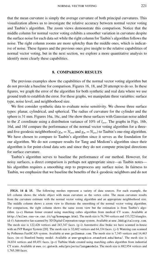
FIGS. 14 & 15. The following meshes represent a variety of data sources. For each example, theleft column shows the whole object with mean curvature as the vertex color. The mean curvature resultsfrom the curvature estimate with the normal vector voting algorithm and an appropriate neighborhood size.The middle column shows a zoom view to illustrate the smoothing of the normal vector voting algorithm.For comparison, the right column shows the same zoom view but the estimation is from Taubin’s algo-rithm. (a–c) Human femur created using marching cubes algorithm from medical CT scans. Available athttp://miles.cnu-ce.cnr.it/cg/homepage.html. The mesh size is 76,794 vertices and 153,322 triangles.(d–f ) Automotive fan scanned by 3D Digital Corporation range system. Available at www.3ddigitalcorp.com.The mesh size is 122,426 vertices and 243,347 faces. (g–i) Automotive disc brake we have scanned in-housewith an IVP Ranger System [20]. The mesh size is 32,602 vertices and 64,334 faces. ( j–l) Watering can scannedby Polhemus FastSCAN system. Available at www.polhemus.com. The mesh size is 7,345 vertices and 14,463faces. (m–o) Stanford bunny model. Available at www-graphics.stanford.edu/data/. The mesh size is34,834 vertices and 69,451 faces. (p–r) Turbine blade created using marching cubes algorithm from industrialCT scans. Available at www.cc.gatech.edu/projects/largemodels. The mesh size is 882,954 vertices and1,765,388 faces.

222 PAGE ET AL.

FIG. 16. Algorithm comparison for synthetic surfaces with Gaussian noise added. The variance of the noisedistribution is 10% of lave. The comparison graphs show the normal vector voting algorithm with a three- anda five-geodesic neighborhood size (gm = 3lave and gm = 5lave) compared to the original algorithm of Taubin. Thegraphs are bin plots with log scales, and each mesh contains 1,024 vertices and 1,922 triangles. (a,b) Planar surface,(c,d) cylindrical surface, and (e,f ) spherical surface.

competitively compare the algorithms. To do so, we would need to select and implementan appropriate smoothing algorithm.

We look at the normal estimation for the plane in Fig. 16b. The percentage error in thisgraph is

err = (1 − ∣

∣N tp Nv

∣∣) × 100%, (18)

where Np = Z is the ground-truth normal and Nv is the estimation. This graph is a histogram


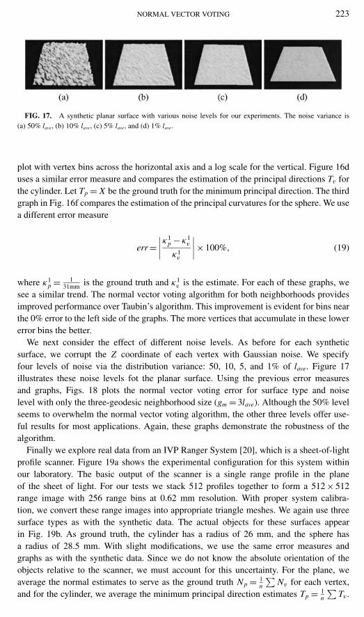
FIG. 17. A synthetic planar surface with various noise levels for our experiments. The noise variance is(a) 50% lave, (b) 10% lave, (c) 5% lave, and (d) 1% lave.

plot with vertex bins across the horizontal axis and a log scale for the vertical. Figure 16duses a similar error measure and compares the estimation of the principal directions Tv forthe cylinder. Let Tp = X be the ground truth for the minimum principal direction. The thirdgraph in Fig. 16f compares the estimation of the principal curvatures for the sphere. We usea different error measure

err =∣∣∣∣κ1

p − κ1v

κ1v

∣∣∣∣ × 100%, (19)

where κ1p = 1

31mm is the ground truth and κ1v is the estimate. For each of these graphs, we

see a similar trend. The normal vector voting algorithm for both neighborhoods providesimproved performance over Taubin’s algorithm. This improvement is evident for bins nearthe 0% error to the left side of the graphs. The more vertices that accumulate in these lowererror bins the better.

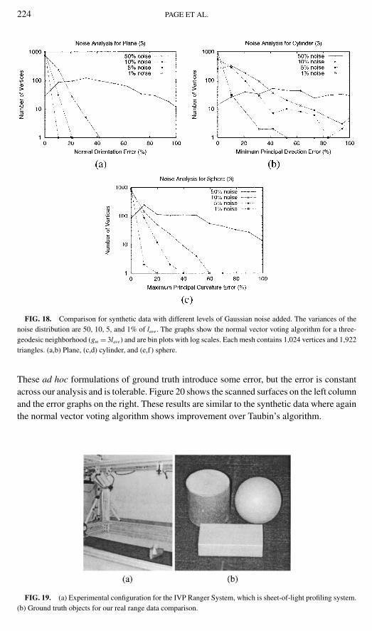
We next consider the effect of different noise levels. As before for each syntheticsurface, we corrupt the Z coordinate of each vertex with Gaussian noise. We specifyfour levels of noise via the distribution variance: 50, 10, 5, and 1% of lave. Figure 17illustrates these noise levels fot the planar surface. Using the previous error measuresand graphs, Figs. 18 plots the normal vector voting error for surface type and noiselevel with only the three-geodesic neighborhood size (gm = 3lave). Although the 50% levelseems to overwhelm the normal vector voting algorithm, the other three levels offer use-ful results for most applications. Again, these graphs demonstrate the robustness of thealgorithm.

Finally we explore real data from an IVP Ranger System [20], which is a sheet-of-lightprofile scanner. Figure 19a shows the experimental configuration for this system withinour laboratory. The basic output of the scanner is a single range profile in the planeof the sheet of light. For our tests we stack 512 profiles together to form a 512 × 512range image with 256 range bins at 0.62 mm resolution. With proper system calibra-tion, we convert these range images into appropriate triangle meshes. We again use threesurface types as with the synthetic data. The actual objects for these surfaces appearin Fig. 19b. As ground truth, the cylinder has a radius of 26 mm, and the sphere hasa radius of 28.5 mm. With slight modifications, we use the same error measures andgraphs as with the synthetic data. Since we do not know the absolute orientation of theobjects relative to the scanner, we must account for this uncertainty. For the plane, weaverage the normal estimates to serve as the ground truth Np = 1

n

∑Nv for each vertex,

and for the cylinder, we average the minimum principal direction estimates Tp = 1n

∑Tv .

224 PAGE ET AL.

FIG. 18. Comparison for synthetic data with different levels of Gaussian noise added. The variances of thenoise distribution are 50, 10, 5, and 1% of lave. The graphs show the normal vector voting algorithm for a three-geodesic neighborhood (gm = 3lave) and are bin plots with log scales. Each mesh contains 1,024 vertices and 1,922triangles. (a,b) Plane, (c,d) cylinder, and (e,f ) sphere.

These ad hoc formulations of ground truth introduce some error, but the error is constantacross our analysis and is tolerable. Figure 20 shows the scanned surfaces on the left columnand the error graphs on the right. These results are similar to the synthetic data where againthe normal vector voting algorithm shows improvement over Taubin’s algorithm.

FIG. 19. (a) Experimental configuration for the IVP Ranger System, which is sheet-of-light profiling system.(b) Ground truth objects for our real range data comparison.


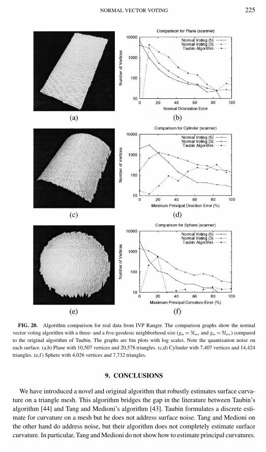
FIG. 20. Algorithm comparison for real data from IVP Ranger. The comparison graphs show the normalvector voting algorithm with a three- and a five-geodesic neighborhood size (gm = 3lave and gm = 5lave) comparedto the original algorithm of Taubin. The graphs are bin plots with log scales. Note the quantization noise oneach surface. (a,b) Plane with 10,507 vertices and 20,578 triangles. (c,d) Cylinder with 7,407 vertices and 14,424triangles. (e,f ) Sphere with 4,026 vertices and 7,732 triangles.

9. CONCLUSIONS

We have introduced a novel and original algorithm that robustly estimates surface curva-ture on a triangle mesh. This algorithm bridges the gap in the literature between Taubin’salgorithm [44] and Tang and Medioni’s algorithm [43]. Taubin formulates a discrete esti-mate for curvature on a mesh but he does not address surface noise. Tang and Medioni onthe other hand do address noise, but their algorithm does not completely estimate surfacecurvature. In particular, Tang and Medioni do not show how to estimate principal curvatures.

226 PAGE ET AL.

Our algorithm completely estimates surface curvature, including principal curvatures, anddoes so in a robust manner despite surface noise.

Two additional contributions of this research are the application of geodesic neighbor-hoods to large meshes and a new surface classification scheme for smoothness discontinu-ities. The normal vector voting algorithm allows the user to specify a geodesic distance thatbounds the voting neighborhood of the algorithm. To generate these neighborhoods, we havemodified Kimmel and Sethian’s fast marching algorithm [21]. This algorithm, and geodesicoperations in particular, should be of interest to other 3D modeling applications beyond ourcurvature algorithm. Another contribution is the classification scheme for detecting surfacediscontinuities. Since we assume that our meshes approximate piecewise-smooth surfaces,we must be careful when estimating curvature along, or near, crease discontinuities. Toidentify these creases, we have presented a novel detection scheme that labels each vertexin the mesh as either on a smooth surface patch, along a crease discontinuity, or with nopreferred orientation. This scheme allows us to handle appropriately the corresponding cur-vature singularities that occur. Other computer graphics and computer vision applicationssuch as simplification, smoothing, and segmentation algorithms should find this detectionscheme beneficial as well.

We have presented results for our algorithm using both synthetic and real data sets. Forthe synthetic data, we have used controlled experiments with ground truth to evaluate theperformance of the algorithm with respect to varying levels of noise. For the real data, wehave generated meshes within our laboratory using an IVP Ranger imaging system and haveused online data from a wide variety of sources including medical and industrial scanners.The emphasis for each data set is a large dense triangle mesh with different degrees ofmeasurement noise across the entire data set. In addition to a qualitative analysis of ourresults, we have presented an in-depth quantitative analysis as well. In particular, we havedirectly compared the results of our algorithm to Taubin’s original algorithm [44]. As aside note, since Tang and Medioni [43] formulate their algorithm for point clouds and sincethey do not estimate principal curvatures, we do not compare our algorithm to theirs. Thesuccess of these results demonstrate the stable and robust performance of our algorithm inthe presence of different types of surface noise.

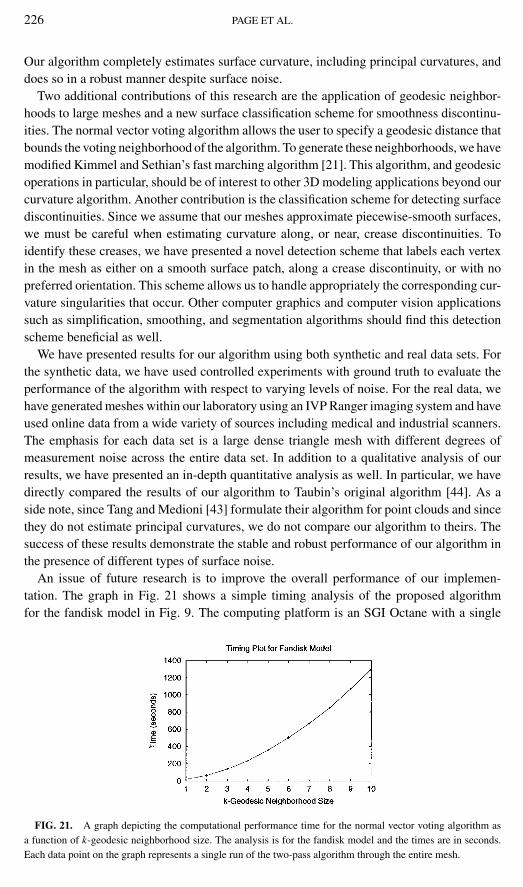
An issue of future research is to improve the overall performance of our implemen-tation. The graph in Fig. 21 shows a simple timing analysis of the proposed algorithmfor the fandisk model in Fig. 9. The computing platform is an SGI Octane with a single

FIG. 21. A graph depicting the computational performance time for the normal vector voting algorithm asa function of k-geodesic neighborhood size. The analysis is for the fandisk model and the times are in seconds.Each data point on the graph represents a single run of the two-pass algorithm through the entire mesh.


195 Mhz MIPS R10000 processor and 128 megabytes of memory. Although we have notoptimized the current code configuration, the trend in the plot is interesting. As we in-crease the k-geodesic neighborhood with the intent of improving our curvature estimate,the computational time grows non-linearly. The three- and five-geodesic neighborhoodsshow reasonable performance compared to the one-geodesic neighborhood that is equiva-lent to the one-ring algorithm of Taubin. Thus we argue that the improvement in accuracy,as demonstrated in Figs. 16–20, with modest increases in neighborhood size are worth theslight increase in processing time.

For our direct comparison of Taubin’s algorithm to our proposed algorithm, we havechosen not to include smoothing as a preprocessing step for Taubin’s algorithm. Although afair comparison would require such processing, we have argued that our intent is to baselineour algorithm. However, some additional comments might be of interest especially in thecontext of the timing information above. First, preprocessing with a smoothing algorithmrequires additional computation effort. That effort should bring the performance of our largerneighborhoods inline with the combination of smoothing and Taubin’s algorithm. Second,an interesting challenge is the choice of a smoothing algorithm itself since such a choicehas a tremendous impact. In particular, we would be interested in whether the smoothingalgorithm preserves crease discontinuities. Additionally, another question arises with regardto handshaking between a smoothing algorithm and Taubin’s curvature estimation to ensurethat we handle curvature discontinuities properly. Taubin’s algorithm does not address thepossibility of curvature singularities.

In conclusion, the major contribution of this research is a new robust algorithm that esti-mates both principal directions and principal curvatures for vertices of a triangle mesh wherethis mesh is an approximation of a piecewise-smooth surface. This algorithm addresses afundamental problem in differential geometry relative to practical implementation on 3Dgraphical models. The future direction for this research is to employ this algorithm to governboth mesh simplification and mesh segmentation algorithms.

ACKNOWLEDGMENTS

This work was supported by the University Research Program in Robotics under Grant DOE-DE-FG02-86NE37968, by the DOD/TACOM/NAC/ARC Program, R01-1344-18, and by FAA/NSSA Program, R01-1344-48/49.

REFERENCES

1. A. Alrashdan, S. Motavali, and B. Fallahi, Automatic segmentation of digitized data for reverse engineeringapplications, IIE Trans. 32, 2000, 59–69.

2. H. Biermann, A. Levin, and D. Zorin, Piecewise smooth subdivision surfaces with normal control, in ComputerGraphics Preceedings (SIGGRAPH 2000), 2000, pp. 113–120.

3. R. J. Campbell and P. J. Flynn, A survey of free-form object representation and recognition techniques,Comput. Vision Image Understanding 81, 2001, 166–201.

4. X. Chen and F. Schmitt, Intrinsic surface properties from surface triangulation, in Proceedings of the EuropeanConference on Computer Vision, Santa Margherita Ligure, Italy, 1992, pp. 739–743.

5. H. Delingette, Simplex Meshes: A General Representation for 3D Shape Reconstruction, Technical Report2214, INRIA, March 1994.

6. H. Delingette, General object reconstruction based on simplex meshes, Int. J. Comput. Vision 32, 1999,111–146.

228 PAGE ET AL.

7. M. Desbrun, M. Meyer, P. Schroder, and A. H. Barr, Implicit fairing of irregular meshes using diffusion andcurvature flow, in Computer Graphics Proceedings (SIGGRAPH’99), 1999, pp. 317–324.

8. E. W. Dijkstra, A note on two problems in connexion with graphs, Numer. Math. 1, 1959, 269–271.

9. M. P. do Carmo, Differential Geometry of Curves and Surfaces, Prentice-Hall, Englewood Cliffs, NJ,1976.

10. F. Ferrie and M. Levine, Deriving coarse 3D models of objects, in Proceedings International Conference onComputer Vision and Pattern Recognition, June 1988, pp. 345–353.

11. F. P. Ferrie, J. Lagarde, and P. Whaite, Darboux frames, snakes, and super-quadrics: Geometry from the bottomup, IEEE Trans. Pattern Anal. Machine Intelligence 15, August 1993, 771–784.

12. P. J. Flynn and A. K. Jain, Surface classification: Hypothesis testing and parameter estimation, in Proceedingsof the International Conference on Computer Vision and Pattern Recognition, June 1988, pp. 261–267.

13. P. J. Flynn and A. K. Jain, On reliable curvature estimation, in Proceedings of the International Conferenceon Computer Vision and Pattern Recognition, 1989, pp. 110–116.

14. M. Garland and P. S. Heckbert, Surface simplification using quadric error metrics, in Computer GraphicsProceedings (SIGGRAPH’97), 1997, pp. 209–216.

15. R. C. Gonzalez and R. E. Woods, Digital Image Processing, Addison-Wesley, Reading, MA, 1993.

16. M. Gopi, S. Krishnan, and C. T. Silva, Surface reconstruction based on lower dimensional localized Delaunaytriangulations, in Computer Graphics Forum (Eurographics 2000) (M. Gross and F. R. A. Hopgood, Eds.),Vol. 19(3), pp. C467–478,544, 2000.

17. C. S. Gourley, Pattern Vector Based Reduction of Large Multimodal Data Sets for Fixed Rate Interactivity dur-ing Visualization of Multiresolution Models, Ph.D. thesis, University of Tennessee, Knoxville, TN, December1998.

18. H. Hagen, S. Heinz, M. Thesing, and T. Schreiber, Simulation based modeling, Int. J. Shape Modeling 4,1998, 143–164.

19. P. S. Heckbert and M. Garland, Optimal triangulation and quadric-based surface simplification, Comput.Geom. Theory Appl. 14, 1999, 49–65.

20. Integrated Vision Products, Sweden, User Documentation: MAPP Ranger System, Version 1.6, 2000.

21. R. Kimmel and J. A. Sethian, Computing geodesic paths on manifolds, in Proc. Natl. Acad. Sci. 95, 1998,8431–8435.

22. L. C. Kinsey, Topology of Surfaces, Springer-Verlag, New York, 1993.

23. C. Lin and M. J. Perry, Shape description using surface triangulation, in Proceedings of the IEEE Workshopon Computer Vision: Representation and Control 1982, pp. 38–43.

24. P. Lindstrom and G. Turk, Fast and memory efficient polygonal simplification, in Proceedings Visualization’98, 1998, pp. 279–286.

25. W. Lorenson and H. Cline, Marching cubes: a high resolution 3D surface construction algorithm, in ComputerGraphics Proceedings (SIGGRAPH ’87), 1987, pp. 163–169.

26. A. P. Mangan and R. T. Whitaker, Partitioning 3D surface meshes using watershed segmentation, IEEE Trans.Visual. Comput. Graphics 5, 1999, 308–321.

27. R. R. Martin, Estimation of principal curvatures from range data, Int. J. Shape Modeling 4, 1998, 99–109.

28. G. Medioni, M. Lee, and C. K. Tang, A Computational Framework for Segmentation and Grouping, Elsevier,Amsterdam, 2000.

29. J. S. B. Mitchell, D. M. Mount, and C. H. Papadimitriou, The discrete geodesic problem, SIAM J. Comput.16, 1987, 647–668.

30. M. E. Mortenson, Geometric Modeling, 2nd ed., Wiley, New York, 1997.

31. S. M. Naik and R. C. Jain, Spline-based surface fitting on range images for CAD applications, inProceedings of the International Conference on Computer Vision and Pattern Recognition, June 1988,pp. 249–253.

32. B. O’Neill, Elementrary Differential Geometry, 2nd ed., Academic Press, Orlando, FL, 1997.

33. D. L. Page, A. Koschan, Y. Sun, J. Paik, and M. Abidi, Robust crease detection and curvature estimationof piecewise smooth surfaces from triangle mesh approximations using normal voting, in Proceedings of


the International Conference on Computer Vision and Pattern Recognition, Kauai, Hawaii, December 2001,Vol. I, pp. 162–167.

34. U. Pinkall and K. Polthier, Computing discrete minimal surfaces and their conjugates, Experimental Math. 2,1993, 15–36.

35. K. Polthier and M. Schmies, Straightest geodesics on polyhedral surfaces, in Mathematical Visualization(K. Polthier and H. C. Hege, Ed.), pp. 391–409. Springer-Verlag, Berlin/New York, 1998.

36. K. Polthier and M. Schmies, Geodesic flow on polyhedral surfaces, in Proceedings of the Joint Eurographicsand IEEE TCVG Symposium on Visualization, 1999, pp. 179–188.

37. S. Pulla, Curvature Based Segmentation for 3-Dimensional Meshes, Master’s thesis, Arizona State University,Tempe, AZ, 2001.

38. C. Rossl, L. Kobbelt, and H. Seidel, Extraction of feature lines on triangulated surfaces using morphologicaloperators, in Smart Graphics (AAAI Symposium 2000), Menlo Park, CA, 2000, pp. 71–75, AAAI Press,New York.

39. P. T. Sander and S. W. Zucker, Stable surface estimation, in Proceedings of the Eighth International Conferenceon Pattern Recognition, Paris, France, 1986, pp. 1165–1167.

40. P. T. Sander and S. W. Zucker, Inferring surface trace and differential structure from 3-D images, IEEE Trans.Pattern Anal. Mach. Intell. 12, September 1990, 833–854.

41. M. Suk and S. M. Bhandarkar, Three-Dimensional Object Recognition from Range Images, Tokyo, 1992,Springer-Verlag, Berlin/New York.

42. Y. Sun and M. A. Abidi, Surface matching by 3D point’s fingerprint, in Proceedings of the Eighth InternationalConference on Computer Vision, 2001, Vol. 2, pp. 263–269.

43. C. K. Tang and G. Medioni, Robust estimation of curvature information from noisy 3D data for shapedescription, in Proceedings of the Seventh International Conference on Computer Vision, Kerkyra, Greece,September 1999, pp. 426–433.

44. G. Taubin, Estimating the tensor of curvature of a surface from a polyhedral approximation, in Proceedingsof the Fifth International Conference on Computer Vision, 1995, pp. 902–907.

45. R. M. Tookey and A. A. Ball, Estimation of curvatures from planar point data, in The Mathematics ofSurfaces VII, Information Geometers, Winchester, pp. 131–141, 1997.

46. T. Varady and T. Hermann, Best fit surface curvature at vertices of topologically irregular curve networks, inThe Mathematics of Surfaces VI, pp. 411–427, Oxford University Press, Oxford 1996.

47. B. Vemuri, A. Mitiche, and J. Aggarwal, Curvature-based representation of objects from range data, Imageand Vision Comput. 4, 1986, 107–114.

48. M. A. Weiss, Data Structures and Algorithm Analysis in C++, 2nd ed., Addison-Wesley, Reading, MA, 1999.

49. K. Wu and M. D. Levine, 3D part segmentation using simulated electrical charge distributions, IEEE Trans.Pattern Anal. Mach. Intell. 19, 1997, 1223–1235.

50. M. Yang and E. Lee, Segmentation of measured point data using a parametric quadric surface approximation,Computer-Aided Design 31, 1999, 449–457.

Documents

Normal Vector Voting: Crease Detection and Curvature Estimation