,

c 4 M F e C t O l -

NORTH AMERICAN AVIATION, INC. SPACE and INFY)RhrZATION SYSTEMS DMSION

https://ntrs.nasa.gov/search.jsp?R=19660026760 2020-01-03T21:01:46+00:00Z

SATELLITE ORBITAL TRANSFER STUDIES (FINAL REPORT)

Contract No. NAS 8-20238

L

SD 66-iZ3 2

16 A u g u s t 1966

Prepared by Gary A. McCue David F. Bender

Space Sciences

Approved by

Director

NORTH AMERICAN AVIATION, INC. SPACE and INFORMATION SYSTEMS DIVISION

FOREMOD

T h i s report is the concluding technical document required under contract NAS8-20238 ( "Investigation of Problems of Optimum Satell ite Orbital Transfer and Rendezvous1I).

The work described in this report was performed by the Space Sciences Department of the Space and Infor- mation Systems Division, North American Aviation, Inc., during a l4 month period cammencing on June 29, 1965 and ending on A u g u s t 30, 1966.

-ii-

e CONTENTS

I Sect icn

I I1 I11 Iv v VI VI1

I I1 111 Iv V VI

ABSTRACT

RESULTS OF STUDY

REFERENCES

APPENDIX A

Introduction The Optimization Problem Quasilinearizat ion Numerical Solution by Quasilinearization Numerical Results Conclusion References

APPENDIX B

Introduction Problem Fonnulat ion Computer Prograrn Description Preliminary Results Conclusion References

i v

3

4

9

15 16 23 31 40 53 54

56

62 ab 69 94 99 100

-iii- SID 66-1226

8

ABSTRACT

Quasilinearization w a s employed t o solve t w o o rb i t a l t ransfer

problems.

problem which resulted from a variational fornulation concerning optimal

o rb i t a l transfer.

t ra jec tory ' s end points could be assumed t o be at unspecified positions

upon arb i t ra ry coplanar orbits.

limited and capable of controlling thrus t direction and duration ("bang-

bang" t h r o t t l e control).

technique it was possible t o determine t r a j ec to r i e s that minimized the

f u e l required f o r o r b i t a l transfer maneuvers which were acccanplished

a fixed time interval.

which were derived from the corresponding optimal impulsive o r b i t a l

t ransfers , were required f o r convergence of the quasilinerarization pro-

cess.

above techniques then was uti l ized t o generate optlmal t ransfers between

numerous pa i r s of arbi t rary coplanar orbits.

it w a s possible t o make a series of significant ccrmparisons concerning

the velocity changes reguired for corresponding optlmal f in i te - thmst

and optimal impulsive o r b i t a l transfers.

demonstrated t h e existence of optimal t ransfers between llshallouly

intersecting" o rb i t s which required only one thrusting period. These

maneuvers were shown t o be analogous t o the be t te r known optimal one-

impulse maneuver.

The first involves a discontinuous two-point boundary value

The boundary conditions were such t h a t the t ransfer

The vehicle was assumed t o be t h r u s t

Through careful use of the quasilinearization

It was found t h a t accurate initial conditions,

A n E M 7094 double-precision computer program incorporating the

Using the result ing data,

Further numerical investigations

-iv-

t

.I

The second problem concerned finding impulsive transfers in the

general three-body problem.

the quasilinearization technique to solve the two-point boundary value

problem that occurs.

point (position and velocity at sane point along an initial orbit or tra-

jectory) and the arrival point (position and velocity at some point along

a final orbit or trajectory).

fer time and the general nature of the expected transfer (e.g., forward

around the earth to retrograde around the moon).

the impulses required to complete the transfer. The required initial

estimate of the trajectory was produced by a patched conic trajectory

program, but it may also be supplied in as many as ten linear segments.

A computer program was developed by employing

The specified boundary conditions were the departure

it was also necessary to specily the trans-

The problem was to find

SID 66-1224

r . ..E

. ' . * Uncla8sified

. - S a t e l l i t e Orb i t a l Transfer Studiea (Final Report)

Gary A. kCue and David F. Bender

S&ID - Downey

16 August 1966

SID 66-1224

NAS 8-20238

Orbital Transfer Quasilinearizat ion Finite-Thrust Impulsive Transfer Boundary Value Problems Three-Body Problem

Quasil inearizstion was employed t o solve two o rb i t a l t ransfer problems. volves a discontinuous two-point boundary value problem which resulted fran a var ia t ional formulation concerning optimal orb i ta l transfer. t h e t ransfer t ra jec tory ' s end points could be assumed t o be a t unspecified positions upon arb i t ra ry coplanar orbits. controll ing thrust direction and duration ( %ang-bangIl t h r o t t l e control). Through careful use of the quasilinearization technique it was possible t o detexmine trajectori.ea t h a t minimized the fue l required for orbi ta l t ransfer maneuvers which were accomplished in a fixed time interval. It was found that accurate i n i t i a l conditions, which were derived from the corresponding optimal impulsive o rb i t a l transfers, were required for convergence of the quasil inearisation process. a t ing the above techniques then was uti l ized t o generate optimal t ransfers between numerous pair6 of a rb i t ra ry coplanar orbits. t o make a series of significant comparisons concerning the velocity changes required f o r

The first in-

The boundary conditions were such t h a t

The vehicle was assumed t o be thrust limited and capable of

An IBn 7094 double-precision computer program blcorpolc

Using the result ing data, it was possible

corresponding optimal f ini te- thrust and optimal impulsive o rb i t a l transferst. -her numerical investigations demonstrated the existence of optimal transf ers between "shallowlg intersectingrt o rb i t s which required only one thrust ing period. There maneuvers were shown t o be analogous t o the be t te r known optimal one-hpulse maneuver.

3'

The second problem concerned finding hpulsive t ransfers i n the general three-body problem. A computer program was developed employing the quasilinearization technique t o solve t h e two-point boundary value problem that occurs. t h e departure point (position and velocity a t some point along an init ial orb i t or tra- jectory) and the arrival point (position and velocity a t scme point along a final orb i t or t ra jectory) . of the expected t ranafer (8.g.) forward around the earth t o retrograde around the moon). The problem was t o f ind the hpulses required t o complete the transfer. i n i t i a l estimate of the t ra jectory wa8 produced by a patched conic t ra jec tory program, but it may also be supplied in (UJ many P8 t en l i nea r sements.

The specified boundary conditions were

It was also necessary t o specify the t ransfer time and the general nature

The required

Lhriag the past seven yea r s the authors have participated in a

se r i e s of contractual studies of optimal o r b i t a l t ransfer and rendezvous.

Under the initial contract, NAS 8-4, work consisted of fonmrlation and

parameter studies involving coplanar two-impulse t ransfer (Refs. 1 t o 3).

The second contracted e f for t (NAS 8-1582) was devoted t o developing

numerical methods f o r finding t h e absolute minimurm two-inpulse t ransfers

between arbi t rary non-coplanar non-coapsidal e l l i p t i c a l orbits.

work, which is documented in Refs. 4 t o 13, led t o several ccpnputational

methods f o r solving such problems.

(NAS 8-52I.l) produced several refinements t o the previously succearsful

numerical techniques (Refs. I 4 and 15).

of a steep descent numerical optimization program (Refs. 16 and 17). Using

t h i s numerical program, it was possible t o conduct a number of studies

which have now been published (Refs. 17, 18, 19 and 20).

also produced a variational fonmtlation of the f i n i t e t h r u s t optixuwn

o r b i t a l transfer problem (Ref. 21).

solution using an ordinarg Newton-Raphson convergence technique which

was l a t e r found t o be inadequate for this dreuuely scursitiw, p r o b h .

The r e su l t s of this t h i r d contract are smmnarized i n Mf. 22.

T h i s

The th i rd contract i n this ser ies

It also led t o the development

This contract

The fofiaalation was programed f o r

Under t h e current contract ( N U 8-20238) e f fo r t uas concentrated

upon solving the f i n i t e thrust orb i ta l transfer problem and upon an in-

vestigation of impulsive transfer i n the three-body problem.

course of the staaJr both of there problems were sa t i s f ac to r i ly solved

D ~ h g the

-1-

N O R T H AMERICAN AVIATION. INC. SPACE and INFOFUMATION SYSTEMS DIVISION

by e m p l o a a mathematical technique known as quasilinearization (Refs.

23, 24 and 25).

This report presents the resul ts of t h e f i n i t e thrust o rb i t a l t r ans -

fer study as Appendix A.

separate document (Ref. 26).

cribing the formulation and computer program ut i l ized t o produce two-

impulse t ransfer circumstances in the three-body problem.

di t ions fo r t h i s problem were obtained from a patched conic t ra jectory

program which w a s a lso developed as part of t h i s contract effort .

Appendix A w a s previously distributed as a

Appendix B contains a separate paper des-

Initial con-

During the past year it was also possible t o update and revise

several of the computer programs f o r performing numerical studies of

two-impulse transfers in the two-body problem.

now been documented and are available f o r use (Refs. 16, 27, 28 and 29).

These programs have

-2-

SID 66-1224

RESULTS OF STUDY

The numerical resu l t s demonstrated tha t quasilinearization i s a

powerful t o o l fo r the optimization of two-point boundary value problems.

This w a s true of both t h e two-body f i n i t e thrust and the three-body

impulsive transfer studies.

impulsive results offered a good first approximation t o t h e i r f ini te

thrust counterparts.

p r ior impulsive o rb i t a l t ransfer s tudies when generating f ini te thrust

t ra jec tor ies about a single a t t rac t ing center.

t h a t the impulsive three-body t ra jec tor ies would be excellent first

approximations when seeking the i r f i n i t e th rus t counterparts.

d e t a i l s of t h i s work appears as Appendices A and B.

In the two-body problem, it was found tha t

For t h i s reason, it w a s possible t o f u l l y u t i l i z e

This resul t a lso implies

Complete

The success of these studies strongly suggests t h a t t h i s work should

be expanded t o include a three-dimensional formulation of the f i n i t e

thrust o rb i t a l t ransfer problem.

expanded t o include a f i n i t e thrust formulation in three dimensions. In

both instances, the results and computer programs generated under the

current study should prove invaluable.

Also, the three-body work should be

-3- SID 66-1224

REFERENCES

1. Kerfoot, HOP. and B d a r d i n s P.R., " A n a l y t i d i . study of

Satellite Rendezvous". North American Aviation, Inc., MD

59-462, (January 1960).

2. Kerfoot, H.P., Bender, D.F., and De8JardinS, P.R., "Ana-

l y t i c a l Study of Satellite Rendezvous" (Final Report),

North American Aviation, Inc,, MD 59-2'p, (20 October 1960).

3. Kerfoot, HOP, and DesJardine, P.R., "Co-Planar Two-Impulse

Orbital Transfers," ARS --print 2063-61, (9 October 1961).

DesJardins, P.R. and Bender, D.P., "Extended Satellite

fbndezroue Study" (Quarterly Raport), N o r t h Ilmhriuan A r i a -

tion, Ino., SID 61-304, (14 September 1941).

4,

5. D e s J d i n s , P.R. and Bender, D.F., "Sate l l i t e Rendezvous

Study" (Second Quarterly Report), N o r t h Amer ican Ariation,

Inc., SID 61-459, (15 December 1961).

DesJarClins, P.R. and Bender, D.F., "Sate l l i t e Rendeevour

Study" (Third Quarterly Report), North American Aviation,

6.

Inc., SID 62-339, (15 March 1962).

7. I k d a r d i n s , P.B., Bender, D.F., and MuCue, G.A., "Orbital

'Ranefer and Satellite Rendezwrus" (Final Report), North

American Aviation, Inc., SID 62-870, (31 August 1962).

Bender, D.F., t'Optimm Co-Plamr Two-Impulse !l?ransfers

Between Elliptic Orbits, " Aerospace m i n e e r i n g , N o . 10,

p. 44 (October 1962).

8.

-4- s;zB 664224

9. Bender, D.F., "Rendezvous Poss ib i l i t i es With t h e Impulse

of Optimum Two-Impulse Transfer, I t Advancements in Astro-

nautical Sciences (AAS), Vol. 16 (Part b e ) , pp. 271-291

(1963). (Published in IIProgress Report #3 on Studies in

the Fields of Space Flight and Guidance Theory," MSFC,

NASA, Huntsville, Alabama, pp. 138-153, 6 February 1963).

10. McCue, G.A., "Visualization of Functions by Stereographic

Techniques, North American Aviation, Inc., SID 63-170,

(20 January 1963) . 11. McCue, G.A., I'Optimization by Function Contouring Tech-

niques," North American Aviation, Inc., SID 63-171, (10

February 1963). (Presented a t 1963 ACM Conference,

27 August 1963).

12. McCue, L A , , I i @ t i m u m Two-Impulse Orbital Transfer and

Rendezvous Between Inclined E l l ip t i ca l Orbits, I t AIAA

Journal, Vol, 1, No. 8, August 1963. (Presented a t A I A A

Astrodynamics Conference, 20 August 1963. Published i n

"Progress Report #4 on Studies i n t he Fields of Space

Flight and Guidance Theory," MSFC, NASA, Huntsville, Ala-

bama, September 1963).

13. McCue, G.A., "Optimization and Visualization of Functions,"

AIAA Journal, Vol. 2, No. 1, (January 1964).

-5- SID 66-U24

l4. Lee, G., "An Analysis of Two-Impulse Orbital Transfer,

AIAA J., 2, 1767-1173 (1964). (Published in !'Progress

Report #4 on Studies in the Fields of Space Flight and

Guidance Theory," MSFC, NASA, Huntsville, Alabama, pp.

167-212, 19 September 19.63).

15. Lee, Go, "On a Restricted Comparison of Two-Impulse and

One-Impulse Orbital Transfer, North American Aviation,

Inc., SID 63-1026, (Published in llProgress Report #5 on

Studies in the Fields of Space Flight and Guidance Theory,I1

MSFC, NASA, Huntsville, Alabama, 19 September 1963).

16. McCue, G.A., and Hoy, R.C., l!Optimum Two-Impulse Orbital

Transfer Program,11 North American Aviation, Inc., SID 65-

1119, (1 August 1965).

17. McCue, G.A., and Bender, D.F., llNumerical Investigation of

Minhxn Impulse Orbital Transfer," A I A A J., 3, 2328-2334

(December 1965 ) . 18. McCue, G.A., and Bender, D.F., tlOptimum Transfers Between

N e a r l y Tangent Orbits," AAS J., Vol. 13, No. 2, (March-

April 1966).

19. Bender, D.F. and McCue, G.A., llconditions f o r Optimal One-

h p u l s e Transfer," North American Aviation, Inc., SID 64-

1859 ( 1 October 1964).

-6-

20. Bender, D.F., "A Coinperison of One- and IPwo-Impulse I lans-

fer for N e a r l y Tangent Co-Planar Orbits," (Published i n

"Progress &port

an8 Guidance Theory," E(BFc, NASA, Hun t sv i l l e , Alabmr, (19

-ternbar 1963).

on studies i n the Fields of space mat

21. Jurovlcs, S.A., " O r b i t a l Trsnsfer by Optimum Thrust Mrec-

t i on and Duration," North American Aviation, Inc., SID

64-29, (12 February 1964). 22. McCue, G.A., Bender, D.F., and Jurovics, S.A., "Satellite

B?ndezvous Study Summary Fteport," North Aprrican Aviation,

Inc., SID 64-368, (10 March 1964).

23. -, Re, SOar AQe cts of m i U n e a r i z a t i o n , ( ~ o n ~ n e a r

Dif fe ren t i a l Equations and Non linear Mechanics) New York;

Academic Press, Inc., pp. 135-146 (1963).

Belhun, R., Kaglwada, E., and Kahba, R., "Quaailinerr-

ization, S y s t e m Identification and Prediction," RAM) CORP.,

24.

fgrI - 38I.2 PR (August 1963).

25. MoGill, B. and Kenneth, P., "Solution of Variational Pro-

blems by Meam of a Wneralized Bhwton-Ba..bon Operator,"

AIAA J., 2, pp. 1761-1766 (October 1964). 26. M e c u e , G.A., "@asillnearitation Determination of Optimum

Finite-!Phrmt Orbital Rrmsfers, It North Aaericul Aviation,

Inc., SID 66-1278, (29 July 1966).

-7- SID 664224

27. McCue, G.A., snd m e , H.J., "Optimum +hro-Impulse Orbi-

tal Transfer Function Contouriw Program," Xorth ABlbrican

Aviation, Inc., SID 65-ll81 (1 Ekpteniber 1965).

28. Mceue, G.A., hroretsky, M. and DuPrie, H.J., "Fortran IV

Stareogrsphic Function Representation and Contouring Pro-

gram," North American Aviation, Inc., SID 65-1382 (1 Sep-

t e a r 1965)

29. McCue, G.A. and m e , H.J., llImproved Fortran ZV Function

Contouring Program, '' Worth Ammzkan Aviation, Inc., SID

65-672, (1 A p r i l 1965).

.

-8- SID sol224

APF"DIX A*

QUASILINEARIZATION DETERMINATION OF OPTIMUM FINTPE-THRUST ORBITAL TRANSFERS

*Note that this appendix is a separate paper having its own nomenclature, illustrations, references, etc.

-9- SID 66-1224

CONTFNTS

Section

I

I1

I11

Iv

v

V I

V I 1

Page

11

13

l4

INTRODUCT Im 15

THE OPTIMIZATION PROBLEEP 16

Equations of Motion M e r Lagrange Equations Boundary Conditions Corner Conditions

17 19 20 22

QUASILINEARIZATION 23

NUMEBICAL SOLUTION BY QUASILINEARIZATION 31

Computation Technique Initial Conditions Variable Length Storage Table Shifting Storage Table Switch Point Analysis

31 32 34 36 38

IJUMERICAL RESULTS 40

Control Variables 40 Convergence and Validity Tests 43 lknmtum Fuel With Mnal Time Open 45 AV Requirements (Intpulsive Thrust vs.Mnite Thrust) 46 . .

CONCLUSION 53

FUEEREXCES 54

10 sID 66-1224

NOMENCLATURE

J A

B N

C

3 C

D

e

F

G

m

N

n

P N

P

r

T

t

x_

F i r s t Integral

Boundary Condition Vector

Effective Exhaust Velocity

Cmbination Coefficients Required f o r Quasilinearization

Process

Auxiliary Variable Defined by Equation 26

Eccentricity

Thrust

Quantity t o be Minimized (Maximized)

Homogeneous Solution Vectors Required f o r Quasil ineari-

zation Process

Time Derivative Vector

Switching Function

Mass

Number of Different ia l Equations

Quasilinearization It erat ion N u m b e r

Par t icular Solution Vector Required f o r Quasilbeari-

zation Process

Sexnilatus Rectum * Radius

Total Time Required f o r Transfer Maneuver

Time

Dependent Variable Vector

11

*

t

X

hi

P

ti

v

w

Components of Vector X

Angular Velocity (8) Mass Flow Rate

Central Angle

Lagrange M u l t i p l i e r

Radial Velocity

Gravitational Constant

Steering Angle

Argument of Perigee

12

ILLUSTRATIONS

.

Figure

1

2

3

4

5

6

7

8

9

10

11

Page

Coordinate System Definition 4

Jacobian Matrix (Equation 38) 11

Comparison of I n i t i a l and Converged Time

Histories of Several Lagrange Multipliers 21

Variable Length Storage Table (ha) and Table With

Switching Points, t,, Shifted f o r Next I terat ion (4b)

Geometry of an Optimal Finite-Thrust Transfer

Maneuver (Thrust Vectors and Steering Angles are

for an Impulsive Transfer) 27

Steering Angle H i s t o r y Compared t o Corresponding

23

Impulsive Thrust Angles 28

Switching Function Time History 30

Difference in AV Required f o r Fhite-ThNSt and

Impulsive Transfers versus I n i t i a l Thrust-to-

Weight Ratio 33

AV Difference as a Function of the Relative Perigee

Orientation of Two El l ip t ica l Orbits 34

Velocity Change Required f o r Finite-Thrust and

Impulsive Transfers Between " A l m s t Tangentvv Orbits

Switching Function The Historiea f o r Several

35

Transf era &tween vvAlmost Tangent Orbit a 37

13 SD 66-1224

AETRACT

1 -

~ I

I 1

Quasilinearization was utilized to solve a discontinuous two-point

boundary value problem which resulted from a variational formulationconcelning

optimal orbital transfer.

transfer trajectory‘s end points could be assumed to be at unspecified

positions upon arbitrary coplanar orbits.

thrust limited and capable of controlling thrust direction and duration

( llbang-bangll throttle control).

tion technique it was possible to determine trajectories that minimized

the fuel required for orbital transfer maneuvers which were accomplished in

a fixed time interval.

were derived from the corresponding optimal impulsive orbital transfers,

were required for convergence of the quasilinearization process. An IEN

7094 double-precision computer program incorporating the above techniques

then was utilized to generate optimal transfers between numerous pairs of

arbitrary coplanar orbits. Using the resulting data, it was possible to

make a series of significant comparisons concerning the velocity changes

required for corresponding optimal finite-thrust and optimal impulsive

orbital transfers.

existence of optimal transf ers between ttshallowly intersecting” orbit8

which required only one thrusting period.

be WlOgOU8 to the better known optimal one-impulse maneuver.

The boundary conditions were such that the

The vehicle was assumed to be

Through careful use of the quasilineariza-

It was found that accurate initial conditions, which

.

Further numerical investigations demonstrated the

These maneuvers were shown to

I. INTRODUCTION

Certain r e a l i s t i c treatments of the optimum orb i ta l t ransfer problem

lead t o a variational formulation whereh the d i f fe ren t ia l equations have

no exact closed form solution.

point boundary value problem considered here(')indicated t h a t it w a s

extremely sensit ive and could not be solved by an ordinary Newton-Raphson

method.

allowed the successful computation of optimal "finite-thrust ' ' transfer

t r a j ec to r i e s between arbi t rary pairs of coplanar e l l i p t i c a l orbits. How-

ever, successful application of quasilinearization w a s found t o depend

upon t he proper use of in i t ia l conditions derived fran an optimum two-

Prior experience with the par t icular two

Reformulation and application of 'tquasilinearization"(2s3s4)

impulse transfer maneuver. (5,6,7,8)

11. THE OPTIMIZATION PROBLEM

The problem t o be considered here involves transferring between a

pa i r of coplanar orb i t s defined by t h e i r semi-latera recta (p1,p2),

eccentr ic i t ies (el,e2) and arguments of perigee (w~,w*) .

is the determination of tha t trajectol-g which resu l t s i n an orb i t a l transfer

What i s required

with minirmrm fue l expenditure.

three-dimensional derivation originated by Jurovics(l) and is similar t o

t h a t presented by Leitmann. ( 9 )

The formulation is a modified version of a

Solution of t h i s optimization problem in-

volves the minimization of a functional which is a function of only the

boundary values of the s t a t e variables: i.e, position, velocity, mass and

time . The function t o be minimized is the character is t ic velocity:

where,

and, where the s t a t e variables are:

In the above expressions c = effective exhaust velocity; r = radius,

= central angle; m = mass, and the subscripts 0 and T refer t o i n i t i a l

and final points of the trajectory.

The rocket and its environment are defined i n accordance with t h e

following assumptions :

1. The rocket is a variable ~ S S part ic le . +

16 SID 66-1224

. 2. The thrust magnitude (F) is a l inear function of the mass flow

rate (PI:

3. The vehicle is capable of thrust direction and t h r o t t l e control,

and the control i s instantaneous.

Further, the t ransfer maneuver is between two o r b i t s about a single

planet with a spherically symmetrical central gravitational f i e l d .

4.

KQUATIoaSS OF MOTION

In polar coordinates (Figure l), the two second order equations of

motion are: I‘ = - F cos v i: - r$2 + 7 m

where,

I‘ = gravitational constant

v = steering angle measured from loca l ver t ica l

Therre equations may be reduced t o first order fonn, where the new variables

p a n d y are defined a8 follows:

r nr

17

!

! I i j

EULER LAGRAhazE EQUATICMS

The opthum path must sat isfy the above equations of motion.

addition, f o r most conventional rockets, the solution is subject t o t h e

In

L

following co&raints:

c = constant

& 5 p 5

where f3&= 0, and B,, is specified.

In the problem considered here one u t i l i z e s the following additional

constraint t o impose %ang-ban@f control of mass flow rate:

P(P-P-1 = 0

If G is t o possess an extrmum subject t o the constraints imposed by

Equations 7 t o 12 and 14, one mwt require t h e f i r s t variation of the con-

strained functional t o vanish.

equation8 for the bgrange multipliers result:

The following Euler-Lagrange d i f f e ren t i a l

k3 = 0

+ = 3 = - A 1 r

The differential equation for

u s e m form:

also may be written in the following

19 SID 66-1224

The l@switching function" (k), which appears i n Equation 20, governs

thrust on-off control and is defined as follows:

where,

Equations f o r the steering angle ( Y ) are a s follows:

14f: D cos v = (25)

where, D = Jxk2 + lb2r 2

Clearly, the steering angle has no physical significance when the vehicle

is on a coasting arc.

Since the d i f fe ren t ia l equations do not involve time expl ic i t ly ,

one obtains a first integral (Hamiltonian):

XIG + + A,# + h6p + 19 = A

where,

A = constant

These last expressions may be used t o replace one of the mer-Iagrange

d i f fe ren t ia l equations and thereby reduce t h e order of the system by one. .

BOUNDARY CONDITIONS

Note that t h e system is described by 10 equation8 for the variables:

rs 8 s P I 9 s

SID 66-1224 20

L

This system thus requires 10 boundary conditions.

the physics of the problem are:

The seven specified by

P l , e l r q s P2, e2d42,q-J

The remaining boundary conditions can be derived fran the transversality

condition:

One may then obtain t h e following additional boundarg conditions: (1)

m

A soenowhat different form of Equation 27 may also be derived: (1)

F m this folm of the equation, it 58 clear t h a t the Hamiltonian

(A i n Quat ion 20) must be equal t o Qk at the end points.

A # 0 at t = 0, then Equation 24 implies t h a t k(0) = k(T).

M h e r , if

Ha- obtained a System of 10 first-order ordinary di f fe ren t ia l

equations which m u a t yield the requirsd optimal trajectory over a

8pcifI.d tima Interval, 0x10 next observes that the problan is of mlxd

.ad-ralw natura .nd

known at the Mthl point (or fbd point). However, it i 8 m a l l known that

the Ai can be scaled by a po8ltlve constant. (9) n u s , by assigning an

appropriate initial value t o Al, t h e number of unknown initial conditiona

YII r0dua.d to four.

the five Valwa of the at. varhbl.8 aro

SID 66-UUr.

.

CORNER CONDITIONS

For th is particular problem, the corner conditions are such that the

multipliers associated with each of the state variables and A, the first

integral, must have the same value immediately preceeding and foUouing

a corner.

(Ai)- = (\)+ (33)

A+ (34 ) A- =

22 SID 66-1224

111. QUASILINEARIZATION

Having obtained a nonlinear two-point boundaleg value problem, the

powerful method of quasilinearization(2) may be used t o generate the re-

quired numerical solutions.

may be written as a set of ten first-order equations, each of which may

be considered t o be one component of the vector equation:

The previously derived differential equations

where,

X = -

r

I

P

Y

m

A1

k

' 6

s

P

Y

- P

- A - +%L I r

0

23

Note tha t i n the above equations an expression f o r t h e switching

function (k) has been derived f r o m Equation 20 and substi tuted f o r X7.

This substi tution w a s useful since it replaced an unknown function with

one w i t h properties par t ia l ly defined by t h e optimum two-impulse transfer

maneuver.

regarded as a parameter whose t ime history may be obtained without resort-

ing t o numerical integration. I n order t o achieve computational economies

Since X3 is constant throughout a given t ra jectory it may be

the cmputer program required that A

i n the vectors of Equation 36.

be assigned t o t h e last position 3

The quasilinearization method may be regarded a s an extension of

t h e Newton-Raphson method f o r algebraic equations t o ordinary differ-

e n t i a l equations.

his tory of the solution vector, X(")(t) i s known. A Taylor se r ies

expansion about t h i s appraximation, truncated with l inear terms, may

then be made t o obtain the derivative of t h e (n + llst approximation,

Suppose t h a t t h e lfnlthll approximation t o the time

N

i = 1, 2...N

where N is t h e number of d i f fe ren t ia l equations, This is t h e fundamental

In t h i s case the Jacobian matrix equation of quasilinearization. (2,3 1

of p a r t i a l derivatives i s rather involved (Eq.38, Fig.2).

lengthy p a r t i a l derivatives appearing i n the Jacobian matrix appear

as Equations 39.

The more

24 SID 06-1224

c 1

0

0

r 0

0

0

0

0

0

0

-

0

0

0

0

0

0

0

0

0

0

0

0

- 0 I

0

0

0

0

0

0

-

0

0

0

r o tu

I

0

0 0 0

0 0 - I

w

0 0 0

L

N 21, x * lu I

0

0 0

0 0 0

0

4

25 SID 66-1224

t

2 2 a i 2PY

a r c

a A, 2PA6

aY r - - - 2 y A 4 - -

2

26 ,

, solutions may be added ( n+l) Because Equation 37 is linear i n the x i

t o sa t i s fy a l l the boundary conditions. By requiring a par t icular solution

t o sa t i s fy the known i n i t i a l boundary conditions, it is necessary t o gene- *

rate a par t icular solution (Pi) plus as many homogeneous solutions (H

as there are unknown i n i t i a l boundary conditions (4). The correct number

of equations t o solve for the combination coefficients, C i n the remain-

ing four boundary conditions a r e thus obtained:

) ij

3'

4

j=1

( t ) , is evaluated by sunrming the (n+l) The (n+l kt approximation , xi stored values of Pi and Hij:

L

j=1

Lf the process converges it will do so quadratically. ( 2 y 3 ) However,

in order f o r the process t o converge, one must have a suf f ic ien t ly accu-

rate first approximation, X(O)(t), t o the time his tory of t h e solution

vector.

- Convergence of t h e process may be examined by evaluating the

following relationships a t t h e end of each i te ra t ion :

i = 1, 2....N

The abrupt changes i n mass flow rate require special consideration.

Whenever the switching function exhibits a zero (llswitch pointll) the mass

flow rate (& = - p ) must undergo a discontinuous change. This property

SID 66-123

can be expressed by employing a unit s tep function i n the def ini t ion of

P : (10)

where,

as follows:

i = 1, 2 ... N The pi(&(")) term offers no net contribution and may therefore be excluded

from fur ther consideration. Next, observe t h a t a t a switch point t h e

Jacobian matrix w i l l have some non-zero te rns appearing i n the column

containing pa r t i a l derivatives w i t h respect t o the switching function (k).

Note t h a t t h i s i s only t rue at the switch points and t h a t Equation 38 is

val id elsawhere. Thus, Equation 45 becomes:

i = 1, 2....N

Since the switching time is determined by the n ' t h i t e r a t ion wherein

k(") = 0 one obtains:

28 SID 66-1224

t

A t t h i s point it should be noted t h a t only those te rns i n Equation 36

which contain mass flow rate will contribute t o the solution at a dis-

continuity.

expressions of the following form:

Substitution of Equations 36, 43 and 44 in to Equation 47 yields

%+ A x i (n+l) = its-;[ k(")(t) 1 d t , i = 1,2 ... N (49)

where the S i represent arbi t rary constants.

In order t o integrate with respect t o the argument of the de l t a

function one may adopt the following definitions:

k = F( t ) , t = F-'(k)

d t = 2 F-' (k) dk

Equation 49 may now be rewritten and integrated with respect t o k;

dk

Equation 53 now may be applied t o derive the following final

expreeaions for the contributions t o the solution at a corner point:

29 SID 66-122A

where,

cos v C P AP = A t - m

cp sin v A y =

Am = - @ A t

- "PhS AX1 - A t - sin v

2 m r

(54)

During the integration of the par t icular and homogeneous solutions

required by Equation 40, k("+l) will, i n general, be non-zero at the

switch points detezmined from the n ' t h i terat ion. The quantity,At,

defined i n Equation 58 may be regarded as an incremental change i n the

length of a burn period called f o r since k (n+l) is now non-zero at the

switch points.

compensate f o r the changes which will result fran these small changes i n

burning time,

The incremental changes defined by Equations 54 t o 57

The need for t h e abeolute value sign can be established

by considering the physical implications of a non-zero value of k (n+U at

points where k(") = 0.

30 SID 66-122&

IV. NUMERICAL SOLUTION BY QUASILINEARIZATION

COMFVTAT ION TECHNIQUES

Equations 1 t o 58 were programmed i n FORTRAN IV fo r solution by

an IBEl 7094 d i g i t a l computer. A double precision integration program

(Ref. 11) employing Runge-Cutta s tar t ing procedures and a variable

step-size difference integration scheme w a s uti l ized. The current

approximation t o t h e solution, X(n) , as w e l l as P and the H were

generated by integration and stored a t fixed tabular intervals. During c -J’ -

the integration it was necessary t o determine values of the variables

between the tabular points. These intermediate values were obtained

by Sterling interpolation(12) truncated with second differences. The

f i f t y equations for P and the H were integrated simultaneously, re-

Wir ing only one evaluation of gi and the Jacobian matrix a t each

value of time ( t ) .

time (T) t h e combination coefficients, Cj, were evaluated from Equation

(40), and the stored values substituted in to Equation (41) t o obtain

% 4

After the integration was terminated a t the f i n a l

the new approximation: 5 (n+l)

Computation w a s saved by relaxing truncation e r ror requirements

where possible.

i n i t i a l conditions were used f o r P. The contributions of the H t o

X(n+l) -

A t the beginning of each i t e r a t ion the best available

-3 - therefore diminished as t h e process converged. Thus, the accuracies

of t h e H were not as important as t h a t of P. -3 I

Convergence of the quasilinearization process was tes ted by can-

(n+l) at the storage interval according and xi (n) paring the values of xi

t o Equation 42. The en t i r e process described above w a s performed by

31 SID 66-1224

a general purpose quasilinearization subroutine which ut i l ized double-

precision FORTRAN N . (11)

INITIAL CONDITIONS

The extreme sensi t ivi ty of the o rb i t a l t ransfer maneuvers con-

sidered here was promptly discovered. For instance, small changes in

tha diiratitns of t h e thrust periods were found t o produce large

variations i n the trajectory,

the process t o diverge. It was therefore necessary t o obtain a real-

i s t i c approximation t o the optimal t ra jectory pr ior t o the in i t i a t ion

of the quasilinearization computations.

Such small variations would often cause

It w a s found t h a t the optimum two-impulse orb i ta l transfer yielded

an excellent in i t ia l approximation t o i t s f i n i t e thrust counterpart.

Accordingly, an i n i t i a l conditions subroutine which ut i l ized a steep

descent numerical optimization program (Refs. 8 and 13) was employed

t o generate an i n i t i a l approximation t o t h e trajectory: X(O). - This pro-

cedure yielded excellent time histories f o r the s t a t e variables r,

8, p , y and m. Utilizing Equation 1, and noting the impulses (velocity

change) given by the two-impulse program, it was possible t o accurately

predict t he duration of each "burn period".

the change i n mass associated with the burn period,and tha t one m u s t

specify a set of rocket parameters; e.g. specific impulse, exhaust

velocity, MSS flow rate, etc.)

d i t ions it was assumed that the impulsive take-off and a r r iva l points

occurred at the center of each burning period.

(Note that one first obtains

In order t o generate the i n i t i a l con-

To avoid having a thrust in i t ia t ion or termination point occur at

t = 0 or t = T, a coasting a rc of several hundred seconds duration

32 SID 66-124-

c

?

w a s assumed t o occur a t t h e beginning and end of the f i n a l optimal

trajectory.

compute exact init ial and f i n a l values of the first four state variables.

An i n i t i a l approximation t o t h e t o t a l time ( T ) required for the maneuver

w a s obtained by summing t h e transfer times corresponding t o the three

impulsive coasting arcs.

Under t h i s assumption it w a s a straightforward matter t o

Although the ini t ia l shape of the switching function ( k ) w a s un-

known the impulsive solution gave an excellent approximation t o the

"switch points" (i.e., k = 0).

t h a t only these c r i t i c a l values of t h e switching function are required

f o r the generation of 5 (k+l).

4 s . 53 t o 58 and by noting tha t t h e Jacobian matrix contains no p a r t i a l

derivatives with respect t o k except a t a switching point.

t ha t 4. 53 also requires an i n i t i a l guess as t o the value of 1; at the

suit ching points .

I n pr ior arguments it w a s established

One may verify t h i s by referring t o

Note, however,

Having detexmined the time histories of the s t a t e variables and the

switching times, it i s also necessary t o supply i n i t i a l approximations t o

the time his tor ies of the Lagrange multipliers. As previously noted, one

Of the h g r m g e multipliers can be employed as a scale factor. Therefore,

A1 was assigned an arbi t rary i n i t i a l value. The following relationship

may then be constructed from Equation 31 by assuming that t = 0 at t h e

impulsive switch point. (7)

33

(59)

SID 66-122.4

,

The impulsive solution may be employed t o determine approximate

values of r, p , y, b , $ and v a t the center of the i n i t i a l burning

period. By pres- an initial value f o r A one may then extract the 3 resul t ing in i t ia l value f o r h6. An i n i t i a l value f o r A then may be 4 computed from the following expression which i s a consequence of Equations

24 and 25:

- A6 ++ r t a n v

-

Thus, the i n i t i a l values of the Laeange multipliers can be estab-

lished by u t i l i z ing the impulsive solution and guessing the ratio. A,/%.

Time his tor ies of the Lagrange multipliers then were produced by an

integration procedure which employed Equations 15 t o 18 and ut i l ized the

previously stored impulsive t h e his tor ies of the state variables. Figure 3

i l l u s t r a t e s the va l id i ty of this procedure f o r a typ ica l computer run by

comparing the in i t ia l and convergedtime h is tor ies of several Lagrange

multipliers. The initial approximations t o the s t a t e variables were con-

siderably better and, i n most cases, differences between ini t ia l approxi-

mations and final converged values could not be detected when plotted t o

the scale of Figure 3. The fact that t he state variables were init ially

w e l l defined was hportant t o achieving convergence of the quasilinearization

technique.

VARIAELE LENCTH STORAGE TABLE

Although straightforward application of quasilinearization will

result i n a solution of the problems considered here, it was found

necessary t o employ a number of refinements t o assure accuracy and

proper convergence. For instance, when storing the tabular values of

34 Su) 66-122+

.

X I T

+ coo

0

- loo

x6

2000 4000 6000 TIME SEC

Mgure 3 - Caanparison of Init ial and Converged T b e Hietories of Several Lagrange MultipHers

35 sID 66-1224

! .

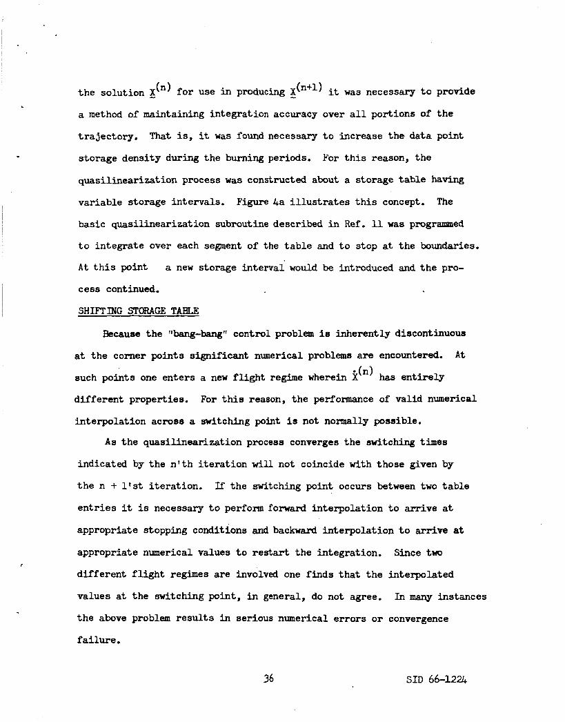
the solution dn) f o r use in producing X

a method of maintaining integration accuracy over a l l portions of the

trajectory.

storage density during the burning periods.

quasilinearization process w a s constructed about a storage table having

variable storage intervals. Figure 4a i l l u s t r a t e s t h i s concept. The

basic quasilinearization subroutine described i n Ref. 11 w a s programmed

t o integrate over each segment of the tab le and t o stop at the boundaries.

A t t h i s point

cess continued.

SHIFTING STORAGE TAHLE

it was necessary t o provide - -

That is, it was found necessary t o increase the data point

For t h i s reason, the

a new storage intervai would be introduced and t h e pro-

Because the llbang-bangll control problem is inherently discontinuous

A t a t t h e corner points significant numerical problems are encountered.

such points one enters a new f l i g h t regime wherein $”) has ent i re ly

different properties.

interpolation across a switching point i s not normally possible.

For this reason, the performance of valid numerical

As the quasilinearization process converges the switching times

indicated by the n’ th i te ra t ion will not coincide with those given by

the n + l’st i terat ion.

en t r i e s it is necessary t o perform forward interpolation t o arr ive at

If the switching point occurs between two table

appropriate stopping conditions and backward interpolation t o arrive at

appropriate numerical values t o restart the integration.

different f l i g h t regimes are involved one finds t h a t the interpolated

values at the switching point, i n general, do not agree.

the above problem resu l t s i n serious numerical errors o r convergence

failure .

Since two

In many instances

SID 66-12U,

4b 1 1 1 1

0

1 1 1 1 1 1 I I I I I I I 1 1 1 1 1 1 1 1 1 1 I

I I . I I I I

I I I I t p

4a 1 1 1 1 I I 1 I I I I 1 1 1 1 1 1 1 1 1 1 1

COAST BURN COAST BURN COAST \ U v 0

Figure 4 - Variable Length Storage Table (4a) and Table With &itching Points, t,, Shifted for Nwrt Iteration (4b)

T

r

37 SID 66-1224

One may employ another %rick” t o insure numerical integration

accuracy at the corner points.

new switching times a re determined which, i n general, w i l l not occur at

t h e previous tabular values.

the new switching times sre used t o define the boundaries of each variable

length storage array.

of quasilinearization wi th the assurance t h a t each stopping point coin-

cides wi th a table entry.

After each i te ra t ion of quasi l inearhat ion

A new table then may be constructed wherein

Tihis makes it possible t o perform a new i t e ra t ion

This newtable and i ts relationship with tha t

used in the pr ior i t e ra t ion is i l lus t ra ted i n Figure 4b. Note tha t t h i s

method eliminates the necessity of interpolating t o obtain the values a t

the stopping points. This numerical continuity across the corner points

was found t o be essential f o r the accurate convergence of the o rb i t a l

t ransfers considered hem.

SWITCH POINT ANALYSIS

As was pointed out ear l ie r , the llbang-banglf control process produces

t ra jec tor ies which are very sensi t ive t o the in i t ia t ion , termination and

duration of thrusting periods.

ra ther sophisticated process f o r determining and controlling the switching

times t o be ut i l ized in the determination of X . h+l> .

It was therefore necessary t o employ a

hr

A numerical procedure f o r determining the zeroes of the switching

function was employed at the end of each quasilinearization i terat ion.

If t h e new switching times showed large deviations f rm the previously

used values, the new times would not be adopted. Instead, the program

would s h i f t the thrust i n i t i a t i o n and telrmination times by a small portion

of the indicated change.

38 SID 66-1224

.

Newly determined switching times would be f u l l y ut i l ized only when

close agreement wi th the previous i terat ion had been achieved.

such close agreement could only be expected t o occur after the quasili-

nearization process had proceeded through several i terations. However,

once t h i s requirement w a s m e t , the program w a s completely free t o use the

switching times indicated by t h e n ' th i t e ra t ion during the computation of

the n + l 'st. The above programed constraints forced the solution t o

conform t o impulsive i n i t i a l conditions u n t i l the process had achieved

suff ic ient convergence t o adequately control i t s e l f .

s t r a in t and without the judicious pse of the impulsive initial conditions

it w a s usually impossible t o obtain convergence.

In general,

.)

Without this con-

39 SID 66-1226

c

.

V. NUMERICAL RESULTS

The forementioned IIM 7094 double precision program was uti l ized t o

generate transfers between a r b i t r a q coplanar non-coapsidal orbits. N m

er ica1 results are best described by comparing the optimal f i n i t e thrust

solutions with corresponding optimal impulsive transfers.

C m O L VARIABLES

As was previously noted, the s ta te 'var iable time h is tor ies produced

from t he impulsive solution showed excellent agreement with the corres-

ponding values f o r the f i n i t e thrust maneuver.

found f o r the control variables.

Initial, f h l and t ransfer orbit8 corresponding t o an optimal f in i te -

thrust t ransfer are depicted i n Figure 5 . The orb i t and vehicle para-

meters a re as follows: P1 = 5,000 m i . , P2 = 6,000 m i . , e = e = 0.2,

w1 =-90°, u2 = +30°, /3 = .OOO1 m,,/sec. and i n i t i a l F/W = 0.4.

indicates the directions and relative magnitudes of t h e two impulses

(El and E2). coincides with its impulsive counterpart when plotted t o the scale of

Figure 5 .

noted.

Similar agreement was

This is best i l l u s t r a t ed by an example.

1 2 Figure 5 also

The transXer orbi t of the optimal f i n i t e thrust transfer

The small arcs over which the engine is burning are also

Figure 6 presents a time history of steering angle, u , for the

orb i t t ransfer maneuver depicted in Figure 5 . Note tha t only a small

portion of the Steer- angle curve has physical significance. These

two portions of the curve are expanded in the inset diagrams of Figure 6.

The inset diagram a lso give the impulsive steering angle f o r ccnuparison

40 SID 66-1224

I-

0 J

- m a

a

w 0 z n

a

LL' ' \

I - ll 0

I . II 0

\ \ \ \ \ \ \ \ \ \ I I I

I I

I /

/ /

/

n

w SID 66-1221*

.

0 O t s! - I

0 0 ol - 0 0 0 - 8 Q

0 I

42

with the f i n i t e thrust solution, F o r t h i s intermediate thrust case, the

t h r u s t i n i t i a t ion and termination times derived fram the impulsive solution

differed by only a few seconds from those indicated by t h e quasilineari-

zation solution.

The switching function f o r t h i s maneuver appears as Figure 7. It

i s clear tha t t h e engine is bum&ng for a .sm=lll pnfi-ior? of the t o t a l

time required f o r the o rb i t a l transfer.

convergence of the quasilinearization process t h e switching times must

In order t o achieve adequate

be determined t o approximately 0.001 seconds.

and noting tha t the maneuver may involve several thousand seconds, one

obtains an appreciation f o r the accuracy which must be maintained.

Furthermore, when one considers t ha t t h i s accuracy must be maintained

during the computations inherent i n Equation 21, it is clear t ha t double

precision arithmetic is a necessity.

CONVERGENCE AND VALIDITY TESTS

Referring t o Figure 7

Several tests of a solution's convergence and val id i ty a re avail-

F i rs t , because the best approximation t o P(0) i s u t i l i zed f o r able.

each i te ra t ion , the C appearing i n Equation 40 should approach zero as

the process converges.

Another test of Convergence may be performed by noting successive values

N

3 This provides the first t e s t of convergence.

of the si given by Equation 42,

also approach zero, One should also observe the switching times approach-

ing appropriate constant values during successive i terat ions, Also, since

k must be zero at each switch point one should observe appropriate tabular

values of k becoming successively smaller with each i terat ion.

the above convergence c r i t e r i a were achieved during the computation of the

During successive i te ra t ions the si should

A l l of

43 SID 66-1224

+200

0

- 200

-400

- 600

-800

- 1000

- 1200

.

7 THRUST PERIODS r

I I

0 2000 4000 6000 8000

TIME, SEC.

Figure 'i - Switching F'unction Time History

a 4 4 sID 66-1224

solutions presented here.

One may compute certain constants of motion as a test of the

solution's val ia i ty , accuracy, etc.

is given by Equation 27 must remain constant.

possible t o compute energy and angular momentum along the coasting a rcs

and note i f these constants are r ea l ly constant,

presented here, solutions wherein energy and angular momentum remained

constant t o more than eight significant figures were achieved,

accuracy was achieved for t h e Hamiltonian.

would not ordinarily be necessary fo r engineering studies, it was re-

quired f o r the accurate comparison of f ini te thrust maneuvers and t h e i r

impulsive counterparts,

For instance, the Hamiltonian which

O f course, it is also

For a l l of t h e results

Similar

Although t h i s extreme accuracy

As a f i n a l t e s t , the converged solution X ( m ) ( 0 ) , was ut i l ized as

i n i t i a l conditions f o r a straightforward integration of t h e Eu le r Lagrange

d i f fe ren t ia l equations.

compared with t ha t generated by quasilinearization.

t e s t confirmed the val idi ty of the quasilinearization solution.

MINIMUM FUEL WITH FINAL TIME OPEN

The solution produced by t h i s method was then

I n a l l cases this

Because the transfer time (T) derived from the impulsive solution

is s l igh t ly nonoptimal additional computations must be performed t o

determine tha t t ra jectory which i s the-opt imal as w e l l as fuel-optimal.

Since the Hamiltonian may be thought of as the partial derivative of final

mass with respect t o T it is necessary t o adjust T un t i l the Hamiltonian

approaches zero, This was accomplished by perturbing T and computing an

additional fuel-optimal t r a j e c t o q . This required several additional quasi-

l inear izat ion i terat ions. The Hamiltonian corresponding t o each of t he fuel-

45 SID 66-1224

O f l b B l t ra jec tor ies -8 examined and simple linear extrapolation w umod

t o predict a new value of T corresponding t o A = 0. Thus, it was possible

t o compute a t ra jectory fo r which T was ltlocallyil optimal.

AV REQUIF#fENTS (mPULsIVE THRUST vs. FINITE THRUST)

Numerous optimal t ra jector ies w e r e computed in order t o produce a

comparison of optimal impulsive transfers and corresponding finite-thrust

maneuvers. Figure 8 compares the velocity change ( A l l ) required f o r

finite-thrust and two-impulse maneuvers over a wide range of initial

thrust-to-weight ra t ios (F/W). It was produced by beginning wi th the

t ransfer maneuver depicted i n Figure 6 and parametrically varying the

specific impulse (note tha t P was held constant).

log plot of t h i s data showed no devbtion from a s t ra ight l i ne (partrboh) over the

range shown. The f ac t that t h e impulsive o rb i t a l t ransfer i s a very

close approxination t o the f i n i t e th rus t maneuver i s verified by the small

percentage differences i n Figure 8.

The original log-

Another interesting comparison was produced by varying the re la t ive

perigee angle ( A w ) of the two coplanar e l l i p t i c a l o rb i t s of Figure 6.

Figure 9 demonstrates tha t the difference i n velocity change required for

impulsive and the f i n i t e thrust maneuvers exhibits a strong dependence upon

A w .

and non-intersecting orbits.

tangency (Am =

The curve is divided in to two regimes corresponding t o intersecting

Near t he value o f a w which corresponds t o

53O. 1301) t h e curve abruptly, but continuously, changes.

This par t icular phenomenon is best explained by reference t o Figure 10

which contains curves for the two-impulse and f i n i t e thrust maneuvers as

separate plots. Figure 10 concerns a small range o f A u over which the

o rb i t s are "almost tangentf1. Since it was known that the class of "almost

SID 66-1224

I- z w 0

w a n c

z

I .o

ORBIT ELEMENTS:

INITIAL MASS) PER z LL > -

Q, 0.01- - - - -

pI = 5000 mi. e , = 0.2, 0 , = 0

p 2 = 6000 mi. e2 = 0.2, o2 = 120°

MASS FLOW RATE = ( i d 4 x SECOND.

t I 1 I I 1 1 1 1

0.01 0. I I .o INITIAL F / W

Figure 8 - Difference in AV Required for Finite-Thrust and Impulsive Transfers versus Initial Thruat-To-Weight Ratio

47 S D 66-1224

I0.C

I .o

0. I

a0 I

I NTE RSECTl N G (TWO- BURN)

/(ONE - * U R N )

NON- INTERSECTING (TWO-BURN)

\

I I

0 60 120 I80

. Figure 9 - & Difference as a Function of the Relative Perigee Orientation of Two Elliptical Orbits

48 SID 66-1224

t

0 W tn \ I- w w LL

L

I970

I969

I968

1967

I966

I965

I964

1963

A O N E - B U R N T R A N S F E R

0 T W O - B U R N T R A N S F E R

L BURNr-j O N E

I TRANSFERS

TWO-IMPULSE' +IMP.+ I T R A N J

- 53.0 - 53.2

Figure 10 - Velocity Change Required for Fhite-ThNst and Impulsive Transfers Between "Almost Tangent" Orbits

SID 66-1224 49

4

.

tangent" orb i t s produced a number of interest ing resu l t s (Refs. '7 and 8 )

considerable effor t was devoted t o accuracy in examining these c r i t i c a l

orientations.

the orb i t s do not intersect and that the curves become separate as inter-

section deepens.

explains t h e abrupt change noted in Figure 9 .

difference depends upon the particular rocket parameters employed (e.g.,

specific impulses, mass flow rate, etc.).

Mote tha t the t w o curves are nearly coincident as long as

This sudden diverging of the two curves i n Figure 10

The magnitude of t h i s

In Refs. U , 15 and 16 the existence of an optimal one-impulse

maneuver was discussed. The two-impulse curve shown i n Figure 10 con-

t a ins a small region over which a one-impulse t ransfer between the two

orb i t s is optimal. The f i n i t e thrust curve is composed of a number of

points which are designated one burn maneuvers or two burn maneuvers.

Note thaL an optimal one burnmaneuver also ex is t s over a small range of

Ab. Thus, one obtains conditions which are again analogous t o those

found f o r impulsive transfer.

As in the impulsive case, the maneuvers represented by points

d i rec t ly on e i ther side of the one burn region a re characterized by

en t i re ly different steering angle, and thrus t time histories. To the

l e f t of the one-burn region t h e first burn period is rather s m d l and

the thrust f o r both burns is i n the forward direction. To t h e r ight of

the o n e h r n region the second burn period is verg small and i t s thrus t

direction opposes the vehicle'svelocity vector. Figure 11 presents the

switching function time h is tor ies associated with each of three kinds

of f ini te thrust maneuvers considered i n Figure 10. For the two burn

transfers the duration of the smaller burn periods was a fract ion of a

50 SID 66-1224

0

- 0.04 k

- 0.08

- 0.12

a. 1 NON- INTERSECTING, TWO-BURN (Aw = - 53?07

- 200 0 400 800 1200 1600 2000

b ) NON-INTERSECTING , ONE- BURN ( A w = -53P12)

0

- 200

- 400

-1 300.5 SEC

-600 ' I I 1 I

0 WOO llpoo Spoo Spoo lQW TIME, SEC

c.) SHALLOWLY INTERSECTING, TWO - BURN (A" = - 5 3 P 1 7 )

Figure U. - Switching Function Time Histories for Several !t'ransfsrs Between "Almost Tangent" Orbits

51 SID 66-1224

t

second as compared to about 300 seconds for the larger burn period. Some

solutions which were near the boundary of the one-burn region exhibited a

second burn period of .002 seconds duration and smaller. The extreme

numerical accuracy required to produce the results of Figure 9 and 10

should be evident.

52 SID 66-1224

. VI. CONCLUSION

t The numerical results demonstrate tha t the quasilinearization

technique can be a powerful t o o l for the optimization of "bang-bang"

control problems.

t i on t o the solution i s required t o insure convergence.

appears tha t impulsive orb i ta l transfer maneuvers provide an excellent

approximation t o t h e i r f i n i t e thrust counterparts. For t h i s reason

most preliminary engineering design studies could be performed with

simple economical impulsive transfer optimization procedures, thus

avoiding a more time consuming and d i f f i c u l t f inite-thrust optimiza-

tion.

However, it appears that a good first approxima-

In general, it

53 SID 66-1224

VII. REFERENCES

1. t

2.

3.

k .

JurovIcs, Stephen A., ttOrbitai Transfer by Optimum Thrust Direction

and Duration, I t North American Aviabion, Inc., SID 64-29 (12 February

1964)

Kalaba, R., Some Aspects of Uuasilinearization,(Nonlinear Differential

Equations and Nonlinear Mechanic6) New York; Acaaemic Press, Inc.,

pp. 13s-I46 (1963).

Bellman, R., Kagiwada, H., and KaLaba, R.,ttQuasFllnearization,Syatem

Identification and Prediction,'' RAND CORP., RM - 3812 PR (August 1963).

McGill, R. and Kenneth, P., llSolution of Variational Problems by

I4eans of a Generalized Newton-Raphson 0perator,lt A I A A J., 2, pp. 1761-

1766 (October 1964).

McCue, G.A., tlOptimum Two-Jmpulse Orbital Transfer and Rendezvous

Between Inclined El l ip t ica l Orbi t s , " A M J., 1, pp. 1865-1872 (1963).

KcCue, G.A., lfOptimization and Visualization of Functions," A I A A J. , 2, pp. 99-100 (Jan- 1964).

McCue, G.A., and Bender, D.F., llOptimUm Transfers Between Nearly

Tangent Orbits,11 North American Aviation, Inc., SID 64-1097 (May 1,

1965 ) . XcCue, G.A., and Bender, D.F., llNumerical Investigation of Minimum

Impulse Orbital "ransfer,lt AIAA J., 3, pp. 2328-2334 (December 1965).

Leitman, G., l l V a r i a t i o n a l Problma With Bounded Control Variable?3,11

Optimization Techniques, edited by G. hitman (Academic Press, New

York) pp. 171-204 (1962).

54 SID 66-1224

c

10. Friedman, B., "Principles and Techniques of Applied Hathcmatics,'l

John Wiley & Sons, Inc. (November 1962).

11. Padbill, J.R., and McCue, G.A., "QASLIN-A General Purpose b s i l i -

nearization Program," North American Aviation, Inc., SID 66-394

(June 1, 1966).

12. Hildebrand, F. B., "Methods of Applied Mathematics, (Ehglewood C l i f f s ,

New Jersey: Rentice-Hall, Inc.) pp. 34-35 (1952).

13. McCue, G.P. and Hoy, R.C., llOptimum Two-Impulse Orbital Transfer

Program," North American Aviation, Inc., SID 65-lll9 (August 1, 1965).

U+. Contensou, P., I1Etude- theorique des t ra jec tor ies optimales dans un

Application au cas d'un center d 'a t t ract ion champ de gravitation.

unique," Astronaut. Acta 8, 134-150 (1963); also Grumman Research

Dept. Translation 7%-22 translated by P. Kenneth (August 1962).

15. Lawden, D. F., Wptimal TraJsctories f o r Space Navigation, Buttelworth8

Scientific Publications Ltd., (London, 1963).

Breakwell, J.V., 1~- Iinpulse Transfer, I' AIAA PFepFint 63-416

( 1963

16.

55 SID 66-1224

APPENDIX %

TWO-IMPULSE TRANSFER IN THE THREE-BODY PROBLEM

q o t e that t h i s appendix i s a separate paper having i t s own nomenclature, i l lus t ra t ions , references, etc.

56

SID 66-1224

r

CONTENTS

Section Page

NOMENCLATURE 58

ILLUSTRATIONS 60

ABSTRACT 61

INTRODUCTION I 62

I1 PROBLEM FORMULATION 64

I11 COMPUTER PROGRAM DESCRIPTION 69

1. Input Data Coordinate Systems 2. Constants 3 . Data &try 4. Program Controls 5 . Time History Storage 6. Initial Time History 7. Subroutine QASLIN 8. Program Output

72 74 75 79 86 87 91 92

Iv

V

VI

PRELIIUNARY RESULTS 9k

CONCLUSION 98

REFERENCES 99

4

57

NOMENCLATURE

A1'A2

G

H

i Y L k

I

J

P

5

Angles of Perigee and Perilune (Figure 4 )

Combination Coefficiezts of Homogeneous Solution Vectors

Earth-Moon Distance (Semi-& jor Axis)

General Symbol for Ekpression f o r Time Derivative of xj, Col.m, vsctor

Universal Constant of Gravitation Times Mass of Earth plus Moon

Homogeneous Solution Vector (of Equation 19)

Unit Vectors Along x,y, z

Impulse r?) Jacobian Matrix

Jacobi Integral

Particular Solution Vector (of Equation 13)

Distance t o E a r t h

Distance t o Moon

Time (Independent Variable )

Time of Travel on Transfer Trajectory

Velocity Vector Components and Magnitude

Position Vector Components

General Symbol f o r Dependent Variable,Column Vector of Dependent Variables

Convergence Values f o r X, a Column Vector

1

The Ratio Mass Moon t o Mass Earth plus Moon

58

SIB 66-1226

w

0

T

t

Angular Velocity of the Moon i n i t s Orbit

Subscripts

For Departure Point a t t = 0

For A r r i v a l Point at t = T

Fer Trmsfer Trajectory

Superscript represents the i te ra t ion number, e.g. x(n>

Underline s ign i f i e s a vector i n three dimensions.

59

SID 66-1224

Figure

1

2

3

4

ILLUSTRATIONS

The Rotating Coordinate System

Flow Diagram for Two-Impulse Computation

Computer Program Output

Patched Conic for Earth t o Moon Trajectory

Page

65

70

80

89

60 SID 66-1224

. ABSTRACT

A computer program f o r finding two-impulse t ransfers between

given tenninal points i n a fixed time i n the three-body problem has

been developed.

i s imagined t o be a space ship,exerts a negligible a t t rac t ion on the

two large centers.

t ra jectory and uses the quasilinearization process t o correct the

t ra jectory so tha t t h e two-point boundary value problem is solved. The

program and i t s use a re described i n d e t a i l and preliminary resu l t s

showing excellent convergence properties are presented.

The only rest r ic t ion i s tha t the th i rd body,which

It generates a Fatched conic t o use as an i n i t i a l

\

1.

61 SID 66-1224

I. INTRODUCTION

Suppose it i s desired tha t a spaceship on some orb i t i n Earth-

Moon space transfer t o a new orbit by means of a two-impulse maneuver.

While t h i s problem is topologically similar t o two-impulse transfer i n

the two-body problem there are t w o significant differences from the

computational and analytic points of view.

o rb i t s a r e not generally cyclic and points along them cannot be re-

presented by f ive o rb i t a l elements and an angle,

of position and velocity are used instead.

i s tha t the given information concerning the departure and a r r iva l points

does not permit one t o describe transfer orb i t s as a known function of

any one parameter,

through two given points and i n the two-body case one can choose, f o r

example, the semi-latus rectum of the t ransfer orb i t a s t he parameter.

It is then possible t o immediately compute the orbi t , the veloci t ies

a t both ends, and t h e impulses.

chose

the parameter.

the impulses, i s a major problem.

the work t o provide a computer program t o compute these quantities.

That is, from the given departure point (Bo i n Figure l), the given

a r r i v a l point ( B i n Figure l), and the given time interval (T), the

program i s t o determine the t ransfer orb i t t ra jectory, the veloci t ies a t

both ends, and the impulses.

In the f i r s t place the

The six components

The second major difference

In general there i s a single in f in i ty of orb i t s

In the three-body case the author

t o span the in f in i ty of orb i t s by using time t o t ransfer as

To obtain the orbit , the veloci t ies a t both ends, and

It w a s the aim of t h i s portion of

T

It was possible t o accomplish th i s for

62

SID 66-1224

the reduced three-body problem i n which the th i rd body does not a f fec t

the motion of the two primarg bodies.

i n e i ther c i rcu lar or e l l i p t i c a l o rb i t s about t h e i r center of mass,

The two large bodies may move

This program represents t h e first necessary s tep i n a longer

range problem which is the numerical analysis of two-impulse t ransfers

i n Earth-Moon space,

of two-impulse t ransfers can be undertaken.

Now t ha t it has been developed a systematic study

SIB 66-1224

c

11. PRO- FORHULATION

The computational problem involved i s a highly non-linear two-point

boundary value problem and the method of solution u t i l i z e s a generalized

Newt on-Raphson") technique which is called quasilinearisation.

In the complete program as it i s described below the input and

output coordinate systems may be centered at the Earth, the Moon, or

t h e i r barycenter and t h e systems may be rotating or iner t ia l . However,

t he computations are all managed i n the rotating system centered a t t he

barycenter and the problem w i l l be described i n this system. The equa-

t ions of motion are eas i ly derived us ing the Lagrangian procedure. Extra

tenus involving C; occur since the rotat ing system usually does not

ro ta te uniformly. W e find:

(l-IJJG(x+ D) - + ;y 2 PG(X-( 1- cl)D 1

3 2 u = 2wv + w x -

S

. x = U . y = v . z = W

As shown in Figure 1 the xy plane i s the plane of t he Earth-Moon motion

and the x axis i s directed toward the instantaneous position of the moon.

G is the universal gravitational constant times t h e t o t a l mass of the

64 SID 66-1224

. *.

. Earth-Moon system, )I equals the mass of the moon divided by t he t o t a l

mass of the system, D i s t h e Earth-Moon distance (or a semi-major axis

of t h e orb i t i f it is e l l i p t i ca l ) , and w is the angular velocity of the

system.

assumed t o be in circular orbi ts t he equations simplify somewhat since

For t h e res t r ic ted problem in which the two primaries a re

= 0 and they possess a w e l l known integrai , the Gacoti kit8grs1,

which i s

r S

Two different uni t systems are provided f o r in the program. One

is based on the metric system using kilometers f o r distance and seconds

f o r time. The second system uses lunar units f o r which w = 1 rad per

unit time, D = 1 lunar distance, and G = 1 (1.d.) /(U.T.) 3 2

Y

EM = D

EO = M D

B, = DEPARTURE (uo, v0t Won X o r Yo.

BT = ARRIVAL (UT, VT, WT, XT, YT, ZT,)

Figure 1. The Rotating Coordinate System

65 SID 66-l-224

. The problem is described as follows.

(xo,yo,zo), the f i n a l position ( ~ , Y T , Z T ) , t h e time (T), and the general

shape of the desired t ransfer trajectory, we wish t o f ind the t ra jec tory

and the veloci t ies a t t = 0 and t = T.

velocity (uto,vto,wt0) at t = 0 which will cause the vehicle t o arrive

a t (+,yT,zT) at the time T l a t e r . The solution i s t o be accomplished

using the quasilinearization procedure which i s described i n Appendix A

Section 111, and in Ref . 1.

(Eqs. 1 t o 6 ) i s of the form of Equation 35 (App.A), and that the feasi-

b i l i t y of using the procedure depends upon finding analytic expressions

f o r the derivatives of the right hand sides (gi) with respect t o the

six variables (X ), Le. , upon obtaining the Jacobian matrix, J.

i s easily accomplished and the matrix f o r the general three-body tra-

Given the i n i t i a l position

T h a t is,we wish t o f ind the

It i s seen tha t t h i s s e t of equations

This 3

jectory i s given in Equation 8.

J= (Jij)

where

0 2 0 0 w 2 - ~ + ~ &+By Bz

wz 2 -A+CZ

($4 -2w 0 0 *+Ep

0 0 0 BZ CYZ

1 0 0 0 0 0

0 1 0 0 0 0

0 0 1 0 0 0

66 SID 66-1224

2 + - '' G (x-(l-p)D) 3(1-~)G(x+ D12 E = +

: r; r' S'

The (n+l) ' th i t e r a t i o n X (n+l), i s obtained as follows from the

n ' t h i t e ra t ion , X(n), and t h e approximate d i f f e r e n t i a l equation (Eq. 37,

App. A i n matrix form):

A par t icu lar integral , P, i s obtained from the previous time h is tory by

integrat ing Equation 13 s t a r t i ng with the initial values f r o m the last

i t e r a t i o n (uo ,vo ,w0 , ~ , y o , z O ) * . A t the same time a set of three

homogeneous solutions t o

(n) (n) (n)

i= J(X(")) H

are generated with i n i t i a l conditions (V1,O,O,O,O,O)*, (0,V2,0,0,0,0)*,

and (0,0,V3,0,0,0)*. The l inea r i ty of Equation 7 i n X (n+l) allows t h e

new i te ra t ion , Equation 10, t o be P plus a l i nea r combination of t he

three solutions.

+ c H ,(n+l) = P + clHl + c2H2 3 3

The coeff ic ients ( c ,c ,c ) are determined by requiring the solution t o

sa t i s fy the boundary conditions at t h e final posit ion (5,yT,zT).

Whe vectors X,g,H and

1 2 3

are rea l ly column vectors but t he initial values a re printed here as rows f o r convenience in typing.

67 sm 664.224

A s explained i n Appendix A (p. 13) convergence of t he process is

examined by evaluating the maXimrrm change ( a t any point) between successive

i te ra t ions in each coordinate (Equation 42, App. A).

Only when every cmponent of 6 has sa t i s f ied given conditions is the

procedure declared t o have converged.

A t the end of each i te ra t ion the impulses are computed at the

beginning and a t the end of the trajectory. We use

If the process converges within the assigned l i m i t of i t e ra t ions

the program transfers t o a mode in which the actual equations are inte-

grated with the complete se t of initial conditions as determined by

QASLIN. The vector, E, now gives the differences between the final

i t e r a t ion and t h i s in tegra l and it will indicate how w e l l this final

in tegra l represents the solution t o the desired problem since the

differences between the coordinates of the final point reached and those

of the given end point a re included in the comparison.

68 SID 66-1224

.

a.

b.

C.

d.

111. COMPUTER PROGRAM DESCRIPTION

A computer program written in double precision FORTRAN IV language

has been developed f o r solving the problem of finding two-impulse trans-

fers between given points i n Earth-Moon space. It was developed t o pro-

vide wide capability arid has the following set af gefieid prtpertfzs:

The initial and f i n a l conditions can be given i n any two of a ser ies

of coordinate systems centered a t the Earth or t h e Moon or t he bary-

center.

o rb i t s are permissible.

Two u n i t systems are presently available: metric with kilometers and

seconds o r lunar units with o = D = G = 1 (see Equation 1-6 above).

The t o t a l t r i p time, however, must be given in hours. Provision f o r

a t h i rd system exists i n the program.

provided in a single short subroutine and can easily be changed.

Real time with the i n i t i a l epoch i n modified Julian Days may be used

and the Moon's posit ion will be determined by the program.

motion of the lunar orbi t node and perigee during the t r i p time a re

neglected.

i n i t i a l position anywhere i n i t s orbit .

The orb i t s of t h e Earth and Moon may be assumed t o be c i rcu lar or

e l l i p t i ca l .

Orbital elements f o r close Earth orb i t s and/or close Moon

The actual constants used a re

The secular

O r , an a r t i f i c i a l reference time may be used with the moon's

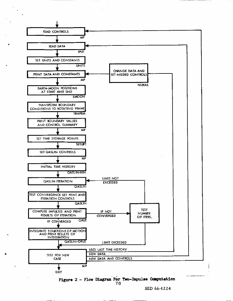
A block diagram of the overall computer program is shown in Figure 2.

The general operation of the program is c lear from t h i s diagram and the

d e t a i l s of using the program a r e described below under the following

69

1

b COMPUTE IMPULSES AND PRINT IF NOT RESULTS O F ITERATION CONVERGED

,

NUMBER OF ITERS.

w

I I I

READ CONTROLS

MP

READ DATA

I PUT

SET UNITS AND CONSTANTS

UNITS

CHANGE DATA AND SET NEEDED CONTROLS PRINT DATA AND CONSTANTS

MP

1 NUKAS EARTH-MOON POSITIONS

AT START AND END EMOON

TRANSFORM BOUNDARY CONDITIONS TO ROTATING FRAME

I TRN FRM 1

I SET QASLIN CONTROLS 1 MP 1

1 I

INITIAL TIME HISTORY 1 QASLIN4IN

QASLIN ITERATION

QASLIN

TEST CONVERGENCE SET PRINT AND ITERATION CONTROLS

1 QASLIN I i w I I

IF CO+ERGED u 1 I

I INTEGRATE EOWTIONS OF MOTION AND PRINT RESULTS OF I INTEGRATION

LIMIT EXCEEDED

USES LAST TIME HISTORY

I TEST F O R NEW NEW DATA

CASE NEW DATA AND CONTROLS r

I J MP

EXIT -- --?-I

Figure 2 - Flow Diagrau-Fir Two-hpulro Ccmputrtion 7 0

SID 664224

headings :

1. Input Data Coordinate Systems

2. Constants

3, Data Entry

4. Program Controls

5 . Time History Storage

6. Initial Time History

7. Subroutine QASLIN

8. Program output

This program has been designed with a great f l e x i b i l i t y for input

conditions,

exceeding the allowable

necessary t o make use of two s l igh t ly d u f e r e n t versions.

obtained by using dummy subroutines when a job is being sent which does

not use a par t icular section. Since the portion of the program f o r the

computations of the init ial time his tory i s used only once for a given

case and is independent of the l a t e r i t e r a t ion process it i s believed t h a t

an overlay process can be developed which W i l l require very l i t t l e extra

computer time,

of time storage points if accuracy requirements should demand an increase.

Unfortunately, at t h i s moment the program is so close t o

storage on the IE44 7094 tha t it has been found

These a re

This would allow a fur ther increase in the t o t a l number

71 SID 66-1224

1. Input Data Coordinate Systems

As already mentioned, the initial and final boundary conditions may be

These are given in Earth centered, Moon centered, or barycentric systems.

specified by the values ICORC(1) = J where: I = 1, 2 for initial, final

conditions; and J = 1, 2, 3 for Earth, Moon, barycenter.

IROTS(1) further identifies the systems according t o the scheme shown in

Table 1.

A secand integer

72

c

J=1 Earth Centered

Rotating 1 x 4 s toward System moon - x y plane

is LOP

\

L

J==3 J=2 Baxycenter

Moon Centered Centered

x axis opposite x axLa ear th toward moon x y plane is LOP xy plane i s

LOP

L

T 2 non rotat ing system

x d s t o w a r d x a i s t o w a r d xaxis moon's orbi t moon's o rb i t toward node on ecliptic node on lunar mo on's

plane is U P equator orb i t node

Cartesian

conditions boundary x d s toward

vernal equinox xy plane i s ec l ip t ic

o rb i t a l elements for boundary conditions

x A s toward not used node

plane i s lunar equator

I xj plane i s UP on ec l ip t i c 1 I

x d s toward vernal equinox q plane is equator

not used not used

same as 3

I same as 2 I same as 2 /not used

same as 3 not used

1 same as i.+ I same as 4 lnot used

73

1

4

2. Constants

The constants used in the program a r e l i s t e d i n Table 2.

were obtained from the American Ephemeris and Nautical Almanac.

(o), semi-jor axis (D) , and G are adjusted t o sa t i s fy o2 = G / g .

Most of them

Mean Rate

TAHLE 2. LUNAR ORBIT AND ASTRONOMICAL CONSTANTS

Eccentricity

Mean Orbital Rate

Incl. LOP t o Ecliptic

Incl. LOP t o Lunar Equator

Incl, Ecl ipt ic t o Earth's Equator

Semi-ma jor axis

Gravitational Constant Times Total Mass

Ratio Mass Moon/Total Mass

Ref . Date. JD 2,439,00005

Asc. Node a t Ref. Date

Asc. Nodal Rate

Perigee a t Ref. Date

Perigee Rate

M e a n Anomaly at Ref. Date

Mean An0rmal;g Rate

.054900489

13.17639 65268 "/day = o

5.1453964'

6.6804O

23.44436O (Epoch of 1950)

384747.87 km = D

403505.3 d / s e c 2 = G

1/82.30 = M

A u g . 28,1965 0 hr. U.T.

69,3226 O

- 0529539222O/d~

5 6 . 5 2 ~ ~

.16435 80025 O/day

41.16000

13.06499 24465 */day

I

4

,

*

3. Data Entry

The procedures used in supplying controls and data t o the program are

shown in Tables 3 and 4.

main program and the data shown in Table 4 are read by the subroutine

INPUT.

in the deck.

The controls shown i n Table 3 are read by t he

The cards of Table 4 follow those of Table 3 with no separation

ard No.

TART3 3. INPUT CONTROL CARD FORMAT

6D12.8

4D12.8

U . 8

3a

6~12.8

6EU. 8

6(E9.3,13

Fortran Symbol

X I ( 1)-XI( 6)

/

XI( 7 )-XI ( 10)

NOSTEP, NINTPl, N ( 4 )

RHOS(l)-RHOS( 6)

RHOS( ?)-RHOS( l 2 )

TSUBT( I),KSUB( I)

I = 1, NIIUTPI

Identification

XI are i n i t i a l values for homogeneous solutions (there are 10 max. ) i n units des- ed.

XERR = controls NOSTEP if NOSTEP = 0

NOSTEP = No. of s teps per time storage interval.

NINTPl = 1 + N o . of time sections(max. 10) N ( 4 ) = print control

RHOS are convergence to l - erances on variables

Time (in hours) at section breaks i n time his tory

Step numbers from beginning (max.value KSUB(NINTPI)) = 125

75

.

t

lard No,

6

7

8

9

10

11

Extra cards as needed f o r i n t egera

Foxmat

1216

6 U . 8

6~12.8

6~12.8

4D12.8

416

361.2

TABLE 3 . con't.

Fortran Symbol

SPARE (1) - (6)

DTI, DTF, DVARI, DVAR2

NCM,NICH( 1)-( 3 )

m( j ) ,DTI(J ) , IDTF(J),IDPT(J), IDDF( J), ICO( J) J=1, NCM

Identification

N(3) = No, of i te ra t ions allowed. NREAD, NQ1, ISETUP not used. N D I F = No. of differences, 3 max, allowed (but see notes) . G?(I) = NQ* of dimensions

(2) = Flag f o r Special problems

(3)-(7) = not used

U s e d t o t ransfer infomation t o subroutines XINM and those it c a l l s ( f i r s t time history section) ,

Increments i n initial, final positions;

initial, final veloci t ies ;

i n i t i a l , final times; two other variables f o r cases using last time history.

NCM = t o t a l number cases based on the initial problem. (max is 30) NICH(~) = control f o r next case; NICH(2),(3) = not used.

NN(J) = case no. (not used) IDTI( J) IDTF( J) IDPT( J ) Integral mult ipl iers IDDF(J) f o r increments ICO(J) These can be -9 to

99.

76

:ard No.

D1

D2

D3

D 4

D5*

Foxmat

TABLE 4. IWUT DATA FORMAT

216, 4I3, 2i6

3 E U . 8

6 U . 8

6m. 8

6~12.8

18UC

--

Fortran Symbol

LOFM, IRAT, ICORC(I),

IMORTA mors( I), ICOEL,

IdentiPication

LORM= 1 Lunar unit = 2 metric units = 3 not specified I R A P 1 real time= 2 artificial time ICORC, IROTS f o r specifying coordinate system (see Table 1) ICOEL = 1 moon's orbit circular = 2 moon's orbit elliptical IMORTA =moon's initial position given in mean (=I) of true (=2) anomaly.

not used

Initial, final position vectors (If orbital elements a, e, incl.)

Initial, final velocity vectors (If orbital elements perigee, node, angle from node ) . Initial, final times' (Hours) N.B. TI must = TSUBT(1) but these do not have to be zero TF must = TSUBT (NINTP1) MOon's initial position: node, perigee, anomaly (DegJ Epoch of time scale for T I and TF in MJD for real the cases,

N1= Number of variables NC = 0 ~ ( 1 ) = no. of points to be connected by linear segments for variable numbered I

77 sID 66-1224

.

4

TABLE 4. INPUT DATA FORMAT con't.

lard No.

D6*

&tra za,ds as needed

Format

D 6 . 3

Fortran Symbols Identification

Z ( K ) , W(K) = (time, value of variable). L i m i t i s 50 pairs

When using linear segments as t he initial estimate of the trajectory-

7 8 SID 66-1224

NOSTEP

4. Program Controls

Use of the program controls and the data input procedure is des-

cribed below.

required by subroutine QASLINwhich can manage a t o t a l of I2 variables

having 10 initial boundary conditions t o be found. In the two-impulse

problem there are either 6 varizbles e t h 3 iii-k~em hitid bmmxtary

conditions f o r a three-dimensional case or 4 variables with 2 unlcnown

initial boundary conditions for t h e two-dimensional case.

of the variables then proceeds as %,*,?.,x,y,z o r jC,f,x,y f o r the three

and two-dimensional situations.

boundary conditions i n the rotating system are printed on the first two

pages of output.

1,2,3,4, r e fe r t o the cards D1, D2, D3, D 4 of Table IV.

A list of variables and t h e i r def ini t ions follows:

Many of the storage dimensions of the variables are those

The numbering

The data and controls along with the

A sample i s included as Figure 3. The card numbers

XI( I> These a re t h e values V1, IT2, V3

non-zero i n i t i a l values used for the ser ies of

homogeneous solutions a s described in the text

following EquaLion 4.

The s t e p s i z e or equivalent, NOSTEP, is

determined from the 5th root unless NOSTEP

is given direct ly .

The number of integration steps per time

storage interval.

desired but a maximum of 3 is suggested since

t h e second order interpolation on the previous

time his tory uses values at the storage points.

etc. of t h e

This can be as large as

79 SID a6-1224

I 1

I

4

i

I

i

1 i

cr b a

. . . . . . c e c

W N L a

b L L

c 3 a 2

m 0

D

0G 0. N OD

4. I

.

h 3 a =i 0 0 0 9 . rl

on 0 01 0

00 30 0' 0 0.0 "I 0 40

l a I

. .

cr h

I 0 3 c) 0 0 CI

0 e

d 0

& 3 0 0 W

d .

cr m I 0 3 0 0 0 0

a 1

.

6 rn

1 0 0 0 0 0 0

0 I

. m

rl d

UJ, u mt Y !

. . . I . . !

SID 66-1224

0 0 0 0 0 0 0 0 0 0 0 0

dodo . * . e

d),Q 0 0 0 0 0

e 4 ' 0 4 0 w ' 1 w

1 %

a o / m o m - 1 I I ' x L L I , ~ n 0 0 0 0 0

. . . . m o r + *

0

I a

Y,OIObO D O ' O O O lsoooo I & . . * .

"10 /N

I d

0

i I

me01 0 m 0. 0' 0

born 0 0 . . &lLd 0001

0 0 0: 909 0 0 01

0 0 cv 0 0 0 1 0 0 0;

1 :

. . .I + 0 '1 m.cD d

0, m ~

I n o 0 0 0 0 0.0 0 0 o o m d o

i m 6 016 0 m o p

0 0 0'0 0 0 o!o 0 0 0,o 0 0 0 0

0 0 0 0 . . . I .

ib L L i ai&

0 0 010

m, r i

m d C r y 0

00 0 0 0 0 0 0 0 0 0.0 0 0 O N

I

.. I

0 .

0 3

m Q ) w m m m 1 1 1

o o c 0 0 0 0 0 0 0 0 0 0 0 0 0 0.J3 . . .e 0 0 0

n n ~

d

. +J - . 5 V

0 Lu n NN O m

mcc a n

0 0 0.0 a 0 0:o

a D a D N O m m 0 I I

0 0 0 0 0 0 c o o m 0 0 0 0 0 0 born 0 0 0

a o n o

. . . O

d I

m

, I

!

! I

I I

i !

I I

I

! i

i

I i

ir i

.

. cn ID n.

. .I a

81

NINTP1 I

RHOS( 12)

TSUBT( I), KSUB( I)

NREAD,NQl, ISFZ'UP

NDIF

The t o t a l time of t he t ra jec tory can be divided

into as many as 9 sections i n each of which the

step-size interval i s constant. NINTPl number

of such sections plus 1.

Print control (each integer above 0 adds the

items l i s tad to the 0;lti;nt)

0 = Final solution is only printed

1 = Time his tory at end of each i te ra t ion

2 = Partial integral (P) and H I S during

integration

The values of the differences of t he variables

t o be compared with the vector 6 . Convergence

i a said t o have occured when f o r every ccanponent

6 L P . The uni t s must correspond t o those

computed by the program a s no conversions are

used . The boundaries of the time storage sections and

the corresponding s tep numbers (times i n hours).

The maximum number of i te ra t ions allowed for

the QASLIN routine.

Not used.

Number of differences used i n the Adams:

Moulton integration (3 maximum allowed). If

larger than 3, 3 is assumed and 4th order

Runge-Kutta-Gill integration will be used for

NDIF steps before the program switches t o t h e

82

SID 66-1221,

SPARE( 1)

SPARE( 2)

SPARE (3

SPARE ( 4 )

Adams-Moulton integration f o r the remainder of

the time.

Number of dimensions of problem (2 or 3).

1-noxmal problem

2-special problem setup. (Dummy at present)

Not used

Used for transfer of information to XZNM and the

subroutines it calls. (The initial time history

section) . If negative the Linear segmented input routine

is called.

center of initial point when barycentered

system is used for init% conditions, Le.,

when ICORC(1) = 3.

Used to give conic center OX f i n a l point when

barycentered system is used f o r final conditions;

i.e., when ICORC(2) = 3.

Angle of perigee of earth centered ellipse

(measured C.C.W. fram direction opposite the

moon) (see Figure 4).

Angle of perilune of moon centered conic,

measured C.C.W. from X axis. (see Figure 4).

RLIM = SPA€E(S)*D (see Figure 4).

Not used.

If positive, used to give conic

SID 66-1224

c

DPI(K), DPF(K) DVI(K), DVF(K) DTI, DTF DVARL, DVAR2

NCM

NIGH( 1)

IDTI, IDTF, IDPI, IDPF, IC0

N I

NC

Increments f o r changes i n boundary conditions

f o r new cases based on the previous case. For

each new case each variable new value = old value

plus increment *ID XX (IDPI i s used f o r both

DPI and DVI and similarly f o r IDPF), DVARI i s

increment i n lunar position, DVAR;! not used,

K = 1, 2, 3

Maximum number of cases based on a given solu-

tion (maximum is 30).

Control f o r new case

1= new data and new controls

2 = new data only

3 = e x i t

Not used

Not used except that f o r NN(NC) = 81, 82

I C O E L is s e t t o 1, 2.

All dimensioned 30, as is NN. These are

integral multipliers f o r increments i n corres-

ponding quant i t ies and they can be from -9 t o

99.

The number of variables of the problem.

T h i s must equal 0.

capability of the subroutine XILS not now

Other values are f o r a

required by t h i s program.

The number of points t ha t detemine the -ear

segments f o r variable numbered I. This is one

more than the number of segments desired. 84

SID 66-12U,

a

(Time, Value) pairs. Note that the time m u s t

be in the units called for by the program and

that the pairs for each variable are grouped

together, Le . the first M(1) pairs refer t o

the M(l)-l sections for the variable p or 2)

85 sID 66-1224

5. Time History Storage

A t the mament the maximum number of storage points is set at 125.

Since the QASLIN integration procedure i s capable of handling a change in

step-size it is permissible t o divide the t o t a l time and the 125 points

in to sections of constant step-size as in Figure b o r 4b, page 37,

Appendix A.

small step-size can be used fo r accuracy because the forces of a t t rac t ion

are large and vary great ly over short distances.

distances longer step-sizes w i l l give equivalent accuracy.

use of the available s teps i s a subject f o r study after the program is

running.

consideration, as noted above, w i l l require some streamlining of the

program so a s not t o exceed core o r the use of an overlay maneuver on

the computer. Very large increases in step-size between sections has

been found unsatisfactory i n tna t the extrapolation fo r new large intervals

is very much less accurate t h a n t h e computation fo r the previous steps.

It is best t o keep t h e step-size change t o a fac tor of two t o four .

This is desirable so that when near the ear th o r moon a

Over the intermediate

The optimal

The t o t a l number of s teps might be increased somewhat but t h i s

86

6. I n i t i a l Time History

In order t o begin the p s i l i n e a r i z a t i o n process it is necessary t o

generate an initial guess f o r the time his tory of a l l the variables (X).

In many cases this can be very crude but f o r highly sensit ive and ex-

tremely non-linear problems t h e first guess may have t o be carefully

made i n order t o obtain convergence on the desired solution. Two-impulse

t ransfer i n t h e three-body problem presents such a s i tuat ion if the tra-

jectory sought is t o t ransfer from the space near one body t o t h a t near

the other.

The motions envisaged fo r study so far have been those f a i r l y close

t o the lunar orb i t plane (LOP). The motion out of the plane has been

assumed t o be l i nea r and decoupled from the motion in the LOP, but a

sinusoidal form could be u t i l i zed with very l i t t l e additional programming

if it is needed.

Three approaches f o r obtaining a first time his torg in the LOP have

been u t i l i zed in t h i s study.

two-for-one Lissajous f igure with variable amplitude t o obtain an approxi-

The first was an attempt t o f ind a simple

mate trajectory. T h i s form did succeed in the case tes ted but required

several i t e ra t ions before the t ra jec tory was rea l ly close t o convergence.

In addition, it w a s f e l t that because one has t o put i n a rb i t ra ry varia-

t ions i n the velocity formulae t o approximate the lunar t ra jec tory

veloci t ies more rea l i s t ica l ly , the technique may not be very satisfactory.

With the hope of reducing the number of i t e ra t ions required f o r

convergence, patched conic procedures were then setup fo r the first t h e

history along with controls so t h a t the various types of Earth t o Moon,

Earth-Earth, Moon-Moon and Moon t o Earth transfers could be studied.

t

In addition a linear segmented time his tory program allowing up t o 50

pa i rs of points t o produce linear segments f o r all variables w a s available

and it was adopted f o r use in this program. All three schemes have been

made t o yield sat isfactory f i r s t time his tor ies , however, because of its

a r t i f i c i a l i t y the first scheme has, f o r the present at least, been dropped

from the program,

Only one comparison between l inea r segmented and patched conic cases

has been made so far and t h i s was f o r an Earth t o Moon t ransfer requiring

4 9 hours,

present as closely as possible the r e su l t s from a portion of a run made

using the Fehlberg three-body problem integration program developed a t

MSFC,

vector of values .OOOO1 ld/ut, .ooOOl ld/ut, .000001 Id, .ooOOOl Id,

The very same problem using the patched conic routine likewise required

8 i te ra t ions t o the same degree of convergence and it did not require any

previous knowledge of t h e trajectory except the general shape, i.e, that

it i s retrograde around the moon,

patched conic technique i s t h e most effect ive one t o use.

The l i nea r segments for t he t ra jec tory were chosen t o re-

Eight i t e r a t ions were needed t o accomplish convergence t o a

Consequently, it is concluded that the

The patched conic scheme has been programmed f o r Earth t o M o m

transfers with retrograde motion around t h e Moon, and f o r Earth-Earth

transfers in which both the initial and final points are on o rb i t s around

the Earth, In all cases themotion is considered t o be on a conic section

in the rotat ing system, tha t is, the computations a re performed i n the

standard

The

Earth t o

rotat ing system and the f a c t t h a t it is not i n e r t i a l is ignored.

specific de t a i l s t o be supplied t o the patched conic routine f o r

Moon t r a j ec to r i e s are the pericenter angles A1,A2, and RLIM as

88 SID 66-1224

. shown in Figure 4.

Y

EARTH ELLIPSE

N O T E : Pi AND P2 ARE PERIGEE AND PERILUNE

Figure 4. Patched Conic Geometry for Earth t o Moon Transfers

These quantit ies a re supplied through the use of SPARE(1) as follows:

A1 = SPARE(3) = Angle of Perigee (Pl) i n Deg.

A2 = SPARE(&) = Angle of Perilune (P2) i n Deg.

RLIM = SPARE(S)*D

I I

/ 1

0 /

/

M

MOON CONIC

The semi-major axis of the Earth section conic is chosen by means of the

formula

a = (.7U - (TF - T I - 80)* .OOl.)*D 1.u.

This was developed t o give a reasonable value for an eighty hour t r i p

89 SID 66-1224

t o the Moon and s l igh t ly higher s&--major axes for shorter t r ips .

scheme was chosen rather than one assuming tha t the period should be

proportional t o t h e t r i p time, since t h i s c a l l s f o r a variation in rrall

of the proper direction as far as energy is concerned,

eccentr ic i ty is determined from t h e ini t ia l point since the true anomaly

is known.

T h i s

Finally the

The Earth section conic is followed u n t i l the distance from the

Earth exceeds the value RLIM,

final one, A = % are used t o dete-the lunar conic.

has been chosen the lunar conic is now fixed and i t s elements are deter-

mined.

conic,

between L and A divided by the remainhg time t o go, thus assuring a r r i v a l

at A a t the proper time,

improper ra te , the velocity time his torg contains the velocity components

corresponding t o the proper rate.

Then the previous point (L) and the

Since perilune

The program can manage e i the r an el l ipse, or a hyperbola f o r t h i s

The m e a n anomaly r a t e is taken t o be the mean anamaly difference

Although t h i s orb i t may be traversed a t an

SID 66-1224

7. Subroutine QASLIN

A double precision subroutine for managing a quasilinearization

operation as outlined in Section I1 above has been developed by McCue

and Radbill (Ref. 2). The details of its use i n the present program are

given in Section I11 (Table 3) and Section IV under the items l i s ted for

the first six control cards.

91 SID 66-1224

8. Program Output

As shown in Fig. 3 , the output consists first of the input data i n

its en t i r e ty and the boundary conditions which include the initial and

final positions of the Moon in its o rb i t as w e l l as the boundary values

f o r the departure point and ar r iva l point of the space ship inlhe rotat ing

bqcefiter system.

In case the ini t ia l time history i s generated by using conic sections,

the o rb i t a l elements of the conics are printed.

i s the initial time history ( i f called f o r ) which is printed by QASLIN

according t o the value of N ( 4 ) a s explained in Section IV (see also

Table 3, card 2).

The next i t e m of output

Then follow the values ( a t t = 0 ) of the Jacobian (J) , the derivatives

(gi), and six other quantities including the distances t o the Earth and

Moon printed by the subroutine JACOB which computes them.

served as a means of checking the computation of these quantit ies and it

T h i s has

remains in the program.

The amount of output per i t e ra t ion is controlled by N(4) as i s ex-

plained above i n Section IV except that when integrating the equations of

motion with the converged values f o r the initial velocity, the pr in t of

t he time his tory i s produced by the subroutine JACOB.

h is tory i s printed (except f o r t h e i n i t i a l time history) t h e value of the

Jacobi in tegra l (Eq. 7) f o r res t r ic ted three-body problem is computed and

printed.

an indication of the accuracy of t he integration techniques.

Whenever a time

The degree t o which t h i s value stays constant (when = 0) i s

The minimum output at the conclusion of an i t e r a t ion consists of a

matrix giving the equations t o be solved f o r c1,c2,c3 (of Fq. Ut), the

92 SID 66-1224

and the vector E . In addition, for this problem the 1’ ‘2’ ‘3 values of c

impulses at both ends are determined and printed each time an output time

history of t he variables is called,

The de t a i l s of t he output can be varied by controls i n the various

subroutines as is indicated by the current usage and the existence of

unused items on the data cards and i n tne labelled common regions of the

program. when the applications of the program are more fully developed

an output plan giving only the needed d e t a i l s can be used.

93 SZD 66-1224

I ’ PRELIMINARY RESULTS

0

t

Two different transfer orbit cases have been used so far i n t e s t ing

The first is a case using lunar units, the boundary condi- the program.

t ions f o r which were taken from two poinlsalong a periodic t ra jectory

canputed with the double precision Fehlberg program.

69.8 hour f l i gh t f rm very near the ear th t o very near the moon using

real time and e i ther two o r three dimensions.

are f o r t h i s second case i n three dimensions.

As has been indicated the variation in the value of the Jacobi

The second is a

The input data of Figure 3

integral along t h e trajectorymay be taken a s a measure of the accuracy

of the trajectory. The values found f o r the final time history as given

by the quasilinearization technique and thosfound by direct integration

of the or iginal equations w i t h the init ial conditions found agree t o the

accuracy of the comparisons given below and thus no dis t inct ion between

them is made.

Fehlberg case (Case 1).

in the time step-sioe in the first of these runs leads t o a substantial

discontinuity i n the value at the change over point.

shows that t h i s d i f f i cu l ty has been almost completely corrected by

keeping the step-size r a t i o under 4.

In Table 5 a r e shown the r e su l t s f o r two runs using the

It can be seen tha t the very large increase

The second run

In order t o maintain a constant value of t h e integral near t h e Earth

o r Moon it i s clear f romth i s table and other similar cases t h a t a small

step-size is needed.

scheme apparently affects t h e variation when near the Earth.

In this case also it is seen t h a t the integration

The step-

94 SID 66-1224

Table 5. Behavior of Jacobi Integral Case 1 (Value from Fehlberg run 2.08602504 (ld)2/(ut)2

Integration Technique*

~- - ! d

Time Step Value of Integral Used at boundary steps Distance to Earth Number Steps (with note) (ld/ut)2 (/and Moon) Id

R w e Kutta G i l l

220 min for 40 steps

Ad- - Moulton

e

2.085 619 1935 (rapid r i se then

2.086 201 1,2lO/. 215 nearly constant )

.0617

I ,0860

7.5 min fo r 24 steps

I I I

I I I

2.087 435

(2: z 3 2.086 036

16.8 min f o r 25 setps

I I

I I

037

023 (low OX))

%(See note on NDIF in Section 4)

120 min 029 0 6 0 0 for 20 steps 029 .943/. 618

210 min 029 . 966/.602 for 20 steps 030 1.203/, 236

38.4 min 030 for 15 steps 2.086 030 1. aO/, 215

;

0973

. 270

i

6omin for 20 steps

024 029

.291 584

95

sm 66-1224

a

sizes of the second run in Table 5 appear t o be sat isfactory for the

intermediate regions.

In the case of the second run of Table 5, the convergence cr i ter ion,

5 , for the difference between successive i te ra t ions was set a t 10- 5

ld/ut f o r each velocity component and at lo4 Id for each position

component. Convergence w a s obtained in 7 i terat ions, each of which

required very nearly -15 minute of computer time.

minute was required f o r the in i t i a l i z ing process including the genera-

t i on of the i n i t i a l time h i s t o r y as a patched conic. Table 6 shows the

behavior of the t o t a l impulse value and the convergence measure for the

last three i terat ions.

the two velocity and position components of t he vector 6 . seen that the convergence r a t e i s extremely good for the last few

i t e r a t ions and that t h e values obtained for the impulse likewise show

strong convergence t o a final value.

In addition a b u t -17

The convergence measures given are the larger of

It can be

The computer time used i s one of the output quant i t ies at each

i t e r a t ion and thus it is possible t o indicate how the computer time i s

used.

cases are given i n Table 7 along with some de ta i l s which influence the

time.

the tab le i n which s a e moderate change in a boundary condition is made

and f o r which the previous time his tory i s modified for the new initial

time history. As expected t h i s new case i s rapidly solved.

procedure can be used for impulsive transfer studies and can be developed

in to a search program f o r finding optimal impulsive t ransfers i n the

three-body problem.

Preliminary time studies showing several runs of the two t e s t s

There are included three runs based on the runs di rec t ly above in

Thus, the

96 SID 66-1224

F

.

:t eration Number

TAHLE 6. IMPULSE AMD CONVERGENCE MEASURE

I

Total Impulse ( w u t 1

-0276 4243 3894

.0276 4094 2633

.0276 4094 2084

1 ld/ut = l.O%km/sec)

Convergence Mea3

V e l . (ld/ut ) re

POS. (Id. )

97 SID 66-1224

n

E: k O Q)d

0, m (d u

0 0

ri li

. .

m 0 4 Ti 8 3 g 3

a 8 0 + 2

98 SID 66-1224

cONCLus1m

A double precision computer program which uses quasillnearization

t o find impulsive t ransfers between given terminals i n the three-body

pmblem has been shown t o give ~ c c w a t e solutforrs xith mmiderable sped.

However, there are still three items t o be completed before the program

can be generally useful: (l), further t e s t s w i l l be needed t o determine

more precisely the controls and limits needed t o produce resu l t s sat isfying

a given accuracy requirement; (2), the development of in i t ia l time history

sections f o r Moon t o Earth t ra jec tor ies and f o r lunar orbit changes is

needed, and (3), the management of the en t i re initial time his tory section

f o r the first case of a se r ies should be controlled by means of an over-

lay process on the computer, thus, allowing an expansion i n the number

of points t h a t can be stored f o r the time history.

c

f

99 SID 66-1224

a 1. McGill, R. and Kenneth, P., "Solution of Variational Pro-

blems by Mean8 of a Oeneralized Newton-lbphson Operator,"

dIAA JaP 2, pp. 1761-1766 (October 1964). 2. Radbill, J.R., and MccUt, G.A., "QASLIN-A General Pur-

pose Quasilinearization Program," North Aarerican Aviation,

Inc., SID 66-394 (June 1, 1966).

100

SID 66-1224