The Impact of Technological Uncertainty on Project Scale

By Kim Oshikoji

Thesis Advisor: Professor Michail Chronopoulos

Master Thesis within the main profile of Energy, Natural Resources

and the Environment

NORWEGIAN SCHOOL OF ECONOMICS

This thesis was written as a part of the Master of Science in Economics and Business

Administration at NHH. Please note that neither the institution nor the examiners are

responsible − through the approval of this thesis − for the theories and methods used, or

results and conclusions drawn in this work.

Norwegian School of Economics

Bergen, Autumn 2015

ii

Abstract

The interaction between uncertainty and managerial discretion is a crucial relationship in a

firm’s investment decision. Particularly, as a disruptive technology can precipitate the failure

of a leading firm, a project under technological uncertainty can largely benefits from an

investment strategy where the potential effects of a disruptive technology can be weighed in

an incumbent technology project’s valuation. Hence, in this thesis, a price-taking firm that

has managerial discretion over both investment timing and the size of a project under price

and technological uncertainty is considered. By constructing an analytical framework, it is

shown that in comparison to solely price uncertainty, a project under low price and

technological uncertainty will have both a lower optimal investment threshold and

corresponding optimal capacity, whereas, under conditions of high price and technological

uncertainty, a project will have a higher optimal investment threshold and corresponding

optimal capacity. Additionally, directly revoking standard real options intuition, it is

established through numerical results that the firm’s optimal investment policy will be

monotonically decreasing as a function of technological uncertainty.

Keywords: real options, capacity sizing, investment analysis, regime-switching

iii

Acknowledgements

I would like to thank Professor Michail Chronopoulos for being my supervisor as well as

instructor for the course ENE422: Financial Aspects of Energy and Commodity Markets.

Under his exceptional guidance and tutelage, I not only completed a major milestone in my

life, but also, because of the manner in which he encouraged me to synthesize and adapt to

new information, attained a love of life-long learning. Additionally, I am thankful for the

kindness and respect he showed me as he was most timely in his critique and never took

more than a week’s time to annotate drafts with helpful comments and suggestions.

Furthermore, I could not be more pleased with his availability as he remained easily

accessible throughout the duration of the semester. Above all, I would like to thank him for

his high standard of academic excellence that is exemplary of this fine institution’s caliber,

which also helped me push my personal boundaries and limits.

iv

Dedication

I would like to take this opportunity to formerly recognize the most kind and caring person I

have ever had both the pleasure and honor of meeting in my entire life. This has been a

person who has given up over two decades of her life to raise me, and also, has never in the

entire history of our relation, ever asked me for anything in return. Hence, it is with great

honor that I am able to dedicate my first, major milestone to my mother Toorandokht Binesh

Oshikoji. I am very much appreciative of everything that you have done for me up until this

point, and I carry the guidance, values, and morals that you instilled in me from a young age

in everything I do. By adapting the sonnet Amoretti LXXV: One Day I Wrote Her Name upon

the Strand by Edmund Spenser, I would like to exemplify to what extent my gratitude goes:

“My verse your vertues rare shall eternize,

And in the heavens write your glorious name:

Where whenas death shall all the world subdue,

Your name shall live, and later life renew.”

Thank you so much.

v

Table of Contents

ABSTRACT..........................................................................................................................................II

ACKNOWLEDGEMENTS .............................................................................................................. III

DEDICATION ................................................................................................................................... IV

1. INTRODUCTION ...................................................................................................................... 1

2. LITERATURE REVIEW .......................................................................................................... 6

3. DISRUPTIVE TECHNOLOGY ............................................................................................. 13

3.1 THE THEORY OF DISRUPTIVE TECHNOLOGY .......................................................................... 13

3.2 LAWS OF DISRUPTIVE TECHNOLOGY ..................................................................................... 16

4. MATHEMATICAL BACKGROUND .................................................................................... 19

4.1 ITÔ’S LEMMA ......................................................................................................................... 19

4.2 MARKOV-MODULATED GEOMETRIC BROWNIAN MOTION ..................................................... 20

4.3 DYNAMIC PROGRAMMING...................................................................................................... 24

5. ANALYTICAL FORMULATIONS ....................................................................................... 28

5.1 ASSUMPTIONS AND NOTATIONS ............................................................................................. 28

5.2 THE MODEL ........................................................................................................................... 30

5.2.1 Regime 2 ..................................................................................................................... 30

5.2.2 Regime 1 ..................................................................................................................... 38

6. NUMERICAL EXAMPLES .................................................................................................... 45

7. CONCLUSION ......................................................................................................................... 50

APPENDIX .......................................................................................................................................... 53

LIST OF REFERENCES ................................................................................................................... 61

vi

This page left intentionally blank

1

1. Introduction

Innovative, dynamic strategies for investments made under the blanket of

technological uncertainty have become increasingly important in recent years with the rise of

disruptive technology. As such technologies are conventionally preliminarily purchased by

the lowest segment of the market as unproved, unpolished products, oftentimes their sale is

associated with a lower price level and, consequently, a lower, expected revenue stream. In

response, incumbent technology firms in the industry are often complacent to their inferior

competitor’s market position. However, in successful cases, where successive refinements

have improved a technology to the extent that it becomes possible to take a significant

portion of market share, a disruptive technology can reshape and revolutionize an entire

industry. Recent examples of such supplantations can be referenced through a widespread

number of cases. For example, classified ads have been replaced by Craigslist; long distance

phone calls are now made with Skype; record stores are going out of business due to iTunes;

research libraries are now at the consumer’s fingertips with Google; Uber is redefining the

entire taxi industry’s business model; and even the most serious of news stations use Twitter

(The Economist, 2015).

Hence, faced with the widespread effects of disruptive technologies, a growing

number of incumbent firms must weigh the difficult choice between holding onto an existing

market by following a repetitive business strategy and risking market share, or by aiming to

capture new markets through embracing disruptive technologies and their risky adoption.

Coined the innovator’s dilemma by Clayton Christensen, the creator of the theory of

disruptive technology (Christensen, 2000), this thesis aims to confront the investment

problem faced by the established firm in order to properly value projects in rapidly changing

industries by examining both investment timing and managerial discretion over project scale.

For capitally intensive projects, discretion over project capacity is particularly crucial, since

the installation of a large project increases a firm’s exposure to downside risk in the case of a

potential downturn in market settings, whereas the installation of a small project limits a

firm’s upside potential if market conditions were suddenly to become favourable

(Chronopoulos et al., 2015). As such, a comprehensive business strategy aimed to counteract

both a potential downturn in market settings and a limitation in upside potential of an

investment project is an important issue for the modern firm.

2

Moreover, historical, empirical evidence further highlights the importance of

managerial discretion in capacity choice. For example, in regards to the case of Kodak, the

rise and fall of this monolithic corporation showcases the vulnerability of even the largest of

firms to negligent capacity investment behaviour. Starting from its monopoly-like

characteristics in the 1970’s during which the firm had achieved an approximate 90% market

share in film and an 85% market share in camera sales in the U.S. (Lucas and Goh, 2009),

Kodak experienced large commercial success in both film and camera sales well into the

1980’s. However, in the proceeding years, with the arrival of Sony’s first electronic camera,

Kodak, rather than prepare for the replacement of film through digital photography, chose to

continually invest in film. This investment strategy continued despite, in 1986, Kodak’s

research labs developed the first mega-pixel camera, one of the milestones that Kodak’s head

of marketing intelligence had forecasted as a tipping point in terms of the viability of

standalone digital photography (Mui, 2012). As a result, in the proceedings years, the

company went from enjoying monopoly-like characteristics to a reduction in labour force by

roughly 80% through retirements, lay-offs, and, finally, filed for Chapter 11 bankruptcy

protection in January of 2012. Exuberantly denoted by Clayton Christensen, for Kodak, the

rise of digital photography was comparable to being hit with a tsunami; the very technology

that Kodak had helped to develop had led to its demise (The Economist, 2012).

Secondly, in the renewable energy industry, technological uncertainty plays a

significant role in wind energy capacity installations as well as its respective valuation. Take

into consideration in 2014, global wind energy capacity installations reached their highest

point in newly installed wind energy capacity recorded to date at approximately 49 GW of

additional global capacity (United Nations Environment Programme, 2015, Huang and

McElroy, 2015). Based on this development, investment trends into wind energy have also

experienced record-setting growth (United Nations Environment Programme, 2015).

Therefore, as capacity installations and investment trends are augmenting, the development

of wind turbine technology is of particular importance to consider within their respective

power plant valuations. According to the McKinsey Global Institute, offshore wind turbine

technology, as it is considerably less developed than onshore wind turbine technology,

shows greater long term deployment potential despite significantly higher capital

expenditure requirements. Similarly, as the offshore wind turbine technology matures, its

costs are hypothesized to drop by more than 50% in capital expenditure requirements and

operating expenses (Manyika et al., 2013). As this implicitly affects the onshore wind

3

turbine market due to technological uncertainty, an onshore wind farm runs a correlated risk

that its level of installations will become economically obsolete due to technological change

before capital costs can be fully recovered and the investment provides positive cumulative

cash flows (Venetsanos et al., 2002). Hence, given these potential long-term, production-

shifting market characteristics and the intrinsic risk in a wind turbine investment, a firm

currently considering investment into wind turbine technology must have the capability to

incorporate a substantial change in onshore wind turbine market conditions as offshore wind

turbine technology matures. Consequently, when considering optimal investment and

capacity sizing from a firm’s perspective into wind turbine technology, a deterministic

valuation at face value provides a significantly inaccurate investment valuation as well as its

resulting decision support information.

Hence, in the aforementioned cases, technological uncertainty plays a key role in the

incumbent technology’s valuation and development strategy. Furthermore, the underlying

effects of disruptive technology highlight the need for responsive and efficient decision

support information in industries as far-reaching as photography to renewable energy that are

forced to deal with the implications of technological change. With relevance to even the

most monolithic of firms, this thesis will examine a firm’s choice in project scale under

technological uncertainty in order to provide a model that can nondeterministically value the

impact technological uncertainty has on project scale. Additionally, price uncertainty will

also be regarded as it plays a direct role in the timing of the capacity investment decision. In

order to construct an appropriate valuation, a real options, regime-switching model is

proposed to effectively incorporate price and technological uncertainty in an irreversible

investment decision. Under these circumstances, the question of how an investment decision

in capacity sizing is affected by price and technological uncertainty is examined.

Presented by Dixit and Pindyck (1994), the real options theory provides a framework

for valuing real assets in uncertain futures. Furthermore, there are two important analytical

dimensions the real options model showcases about an investment problem. First off, a

dynamic representation of the timing of the investment decision is used, whereas, in the

traditional sense, a static timeframe was considered and weighed when making a final

investment decision. Secondly, underlying factors are represented as stochastic processes. As

such, stochastic processes can produce a more accurate representation of movements that

fluctuate randomly and unpredictably. Accordingly, the resulting investment strategy

becomes more restrictive as the strategy takes into further consideration both the qualitative

4

and quantitative implications of the value of waiting for more information about uncertain

future trends (Botterud and Korpås, 2007).

Moreover, regime-switching models often portray the tendency of financial markets

to exhibit volatile behaviour with the phenomenon that the new behaviour often persists for

several periods after a change has occurred. While the characteristics captured by regime-

switching models are oftentimes identified by econometric procedures, they can also

correspond with different periods in regulation, policy, and technological change (Ang and

Timmermann, 2012). As such, regime-switching models can effectively capture the

underlying effects a disruptive technology can have on incumbent technology market

conditions.

Thus, the contributions of this paper are three-fold. First off, in order to derive the

optimal investment threshold and the corresponding optimal capacity, an analytical

framework combining both regime-switching and real options is proposed for investment

opportunities under price and technological uncertainty. Second, in order to more closely

scrutinize immediate investment policy, price and technological uncertainty are examined to

see their interaction with optimal capacity sizing. Third, managerial insight is provided for

capacity investment decisions through analytical and numerical results concerning both the

qualitative and quantitative implications of the interactions between irreversible investment,

disruptive technology, and managerial discretion over project scale.

In addition, the delimitations of the model concentrate solely on basic American call

option characteristics. By doing so, the model forgoes the option to abandon the incumbent

technology project post-investment if a regime-switch has occurred in the incumbent

technology market conditions. As the abandonment option gives the firm the opportunity to

sell a project’s cash flows over the remainder of the project’s lifetime, the investment

decision’s salvation value and, analogously, its American put option characteristics are

ignored. Considering the project’s liquidation value could further affect the project’s optimal

investment threshold and corresponding optimal capacity, it is important to note that the

model serves solely as an approximation tool rather than one with complete precision.

In Section 2, literature regarding the analytical framework will be further evaluated. In

Section 3, evidence supporting regime-switching will be presented through the lens of

Clayton Christensen’s theory of disruptive technology. Then, in Section 4, the mathematical

5

tools implemented in the model will be examined. Subsequently, the regime-switching, real

options model will be built in Section 5. First, investment excluding a regime-switch is

analyzed in Section 5.2.1 where an analytical expression for optimal timing and capacity is

derived. In Section 5.2.2, the penultimate investment decision under both price and

technological uncertainty is examined, and a nonlinear solution requiring the numerical

methods executed in Section 6 are implemented in order to gain managerial insight from the

model. Within the same section, numerical results for the effects of regime-specific price

uncertainty as well as technological uncertainty are regarded in order to illustrate their

interaction with the optimal investment policy. Lastly, in Section 7, concluding remarks,

limitations of the model, and suggestions for future research are offered.

6

2. Literature Review

In this section, literature related to the theoretical background of this paper is

presented. It is systematically reviewed in two steps. First, real options theory will be

broadly examined to present its historical background and its evolution as a framework.

Particular nuance applications will also be observed to arrive at the conclusion of dynamic

programming as the application of choice in the real options framework. Secondly, as this

thesis concentrates on optimal timing and capacity sizing under price and technological

uncertainty, the recent literature surrounding these concepts will additionally be examined.

By doing so, this section aims to highlight the existing gap in academic literature to support

modelling a lumpy investment under price and technological uncertainty with a regime-

switching, real options model.

Real options theory complements the traditional discounted cash flow method, which

originates from the classical work of Fisher (1930). In his valuation method, decision-

making criteria for an investment decision is constructed by discounting the cash flows of a

project in order to find its net present value, which is then subsequently used to evaluate the

project’s potential for investment. If the net present value of the project is positive, the

investment is considered attractive; and in the case that the net present value is negative, the

project is assumed to be unprofitable and abandoned. Conversely, using contingent claims

analysis, Majd and Pindyck (1987) show how the traditional discounted cash flow method

understates the value of an investment project by ignoring the inherent flexibility in the time

to build and, as an outcome, showcase how adhering to the simple net present value rule can

result in gross investment error. Furthermore, the real options framework considered by

Majd and Pindyck (1987) was further implemented by McDonald and Siegel (1986) to

address the standard problem of optimal investment timing in a project of given capacity size

with the perpetual option to invest. Further discrediting the net present value rule, their

findings quantify that for reasonable parameter values, sub-optimal investment timing can

affect a project’s value with a traditional net present value of zero by as much as 10-20%.

Hence, through the acceptance of this criticism, the criteria governing a net present value

calculation can be deemed insufficient, and highlights the necessity for an alternative

investment valuation method.

7

However, although the contingent claims approach aims to fill this gap in literature, its

limitations in assumptions restrict its application to span all investment opportunities. The

standard real options textbook by Dixit and Pindyck (1994) seeks to overcome this

shortcoming by extending the work of Mcdonald and Siegel (see Chapter 5 of Dixit and

Pindyck (1994)) by considering both the contingent claims approach and, a more broader

method, dynamic programming, to the firm’s investment decision. By examining the

relationship between these two approaches at the firm level, the authors highlight their

specific merits for use in the context of irreversible investment and stochastic revenue

streams. First off, contingent claims analysis works to construct a riskless portfolio through

an appropriate long and short position. This portfolio, consisting of both the risky project

and investment assets, tracks the project’s uncertainty (Insley and Wirjanto, 2010). In

equilibrium with no arbitrage opportunities, the portfolio must then earn the risk free rate of

interest, which allows the value of the risky project to be determined. However, the

limitations of contingent claims analysis dictate that any stochastic change in the project’s

value must be spanned by existing assets in the economy and that capital markets are

sufficiently complete so that a dynamic portfolio of assets can perfectly correlate with the

value of the project. In comparison, dynamic programming provides an application that is

considerably more flexible in market parameters and does not require diversification of risk.

Notwithstanding the relaxation of market assumptions, the exogenous discount rate

implemented in dynamic programming highlights its subjective shortcomings. Regardless, in

order to model an incumbent technology market dealing with innovation rates such as that of

a disruptive technology, dynamic programming provides the required flexibility to model a

production capacity investment decision under price and technological uncertainty.

As the breadth of disruptive technology effects are widespread, it is additionally

important to note the numerous industries real options have analyzed and its extensions in

application. Antecedents to the Mcdonald-Siegel investment model include seminal works

by Myers (1977) who studied real option effects on corporate borrowing behaviour and

Tourinho (1979) who pioneered real options application to an exhaustible, natural resource

reserve. Furthermore, the field of real options spans the categories of real estate development

(Titman, 1985, Capozza and Sick, 1994, Quigg, 1993), corporate strategy (Kester, 1984,

Kulatilaka and Marks, 1988), research and development (Morris et al., 1991), and enterprise

valuations (Chung and Charoenwong, 1991, Kellogg and Charnes, 2000), amongst others.

Lastly, real options, petroleum literature is particularly well developed (Ekern, 1988,

8

Cortazar and Schwartz, 1998, Kemna, 1993) given its exceptional fit for oil price uncertainty

and the high stakes nature of petroleum projects. Furthermore, strategic real options

literature provides useful extensions where managerial insight is added in addition to solving

an investment timing problem. Combining the competitive real options model and a Markov-

switching regime, Goto et al. (2012) study the investment problem of two asymmetric firms

in the context of boom and recessive market conditions and find the investment threshold

differences of a firm as a leader and as a follower are regime-dependent. Moreover,

Chronopoulos and Siddiqui (2015) study the conventional investment problem where a firm

considers the optimal time to undertake an investment project under both price and

technological uncertainty. Implementing three different investment strategies: compulsive,

laggard, and leapfrog; they find that under a compulsive strategy, technological uncertainty

has a non-monotonic impact on the optimal investment decision. Hence, extensions and

applications of real options literature are far-reaching while continually providing additional

managerial insight to basic real options applications.

In the area of investment under technological uncertainty, optimal timing problems

show various results with adoption rates of technologies. Early works include Balcer and

Lippman (1984) who analyze the optimal timing of technology adoption using switching

options. They find that the firm will adopt the current best technology practice after a certain

threshold, and, in the case that technological uncertainty is increasing, new technology

adoption will be delayed. Conversely, they also find that it may be profitable to purchase an

incumbent technology that was considered unprofitable at its conception if after a certain

period of time, no technological advances are made. Adopting the dynamic programming

approach from Dixit and Pindyck’s (1994) real options framework, Farzin et al. (1998)

extend the work of Balcer and Lippman (1984) by analyzing the optimal timing of

technology adoption by a competitive firm when investment in new, improved technology is

an irreversible investment decision and technological progress evolves according to a

Poisson process. Including the correction by Doraszelski (2001), they find that a firm will

defer the adoption of a new technology when it takes the value of waiting into consideration.

Introducing both game-theoretic considerations and uncertainty to the real options

framework, Huisman and Kort (2004) study a duopoly model where two firms have the

option to invest in an incumbent technology under the uncertainty that a superior technology

with an unknown arrival rate will become available as an investment option. Modelling the

arrival rate according to a Poisson process and assuming that switching is not an option after

9

investment in the incumbent technology has taken place, they find that investment is further

delayed based on technological uncertainty, and the firm who invest second receives the

highest payoff. Price uncertainty modeled by geometric Brownian motion also plays a

substantial role as it induces a higher probability that the new technology will be adopted

instead of the current technology.

Interestingly, as the predominant source of real options literature deals solely with

investment timing while considering capacity sizing fixed, the strategic consequences of

such a choice undermine the effects of managerial discretion over capacity size, while

predominantly establishing the standard result that uncertainty directly correlates with the

value of waiting. Supporting this switch, in his review of Dixit and Pindyck’s textbook

(1994), Hubbard (1994) states,

“(…) the new view models… do not offer specific predictions about the level of

investment. To go this extra step requires the specification of structural links between the

marginal profitability of capital and the desired capital stock” (page 1828).

As such, henceforth, the real options literature that deals with both optimal capacity sizing

and timing will be reviewed. According to the survey by Huberts et al. (2015), three distinct

areas of this type of literature prevail: continuous time models where investments have a

lumpy structure, discrete time models, and incremental investment models. As the latter two

models go beyond the scope of this thesis’s application, lumpy investment models will be

further regarded.

In the area of lumpy investment strategies in continuous time models, the firm

generally invests at a later point in time and at a larger corresponding capacity size

contradicting how uncertainty conventionally affects the firm’s growth. Early examples

include the work by Manne (1961), who was the first to determine that the firm invests in a

larger capacity level when uncertainty increases by observing a stochastic capacity

expansion problem. Continuing this work, Dangl (1999) sets up a model with both a concave

investment cost function and a deterministic production cost function with price determined

by both production quantity and a demand shift parameter assumed to undergo multiplicative

geometric Brownian shocks. Under these conditions, he finds that increasing levels of

demand uncertainty correlate with a delayed optimal investment strategy and increased

project capacity. In the same year, Bar-Ilan and Strange (1999) examine capital stock as a

10

capacity sizing and timing problem while assuming both clearance over production

flexibility and a deterministic, marginal production cost. In comparison to Dangl (1999),

their output price follows solely a geometric Brownian motion. Furthermore, adopting a

similar method as that established by Dangl (1999), Bøckman et al. (2008) analyze

hydropower projects. Although consistent with the exponential form of the concave

investment cost function as that of Dangl (1999), they choose to model a convex cost

function to match the limitations renewable energy projects conventionally exhibit; as the

chosen capacity approaches a finite maximum capacity, each new unit of capacity displays

diseconomies of scale. The contribution margin, which is indicated as the difference between

electricity price and the marginal production cost, is also modelled by geometric Brownian

motion. Similar to Bar-Ilan and Strange (1999), Kort et al. (2011) model both flexible and

inflexible production in a firm’s capacity investment decision. In order to do so, they assume

clearance in the inflexible firm model, while varying utilization rates of installed capacity in

the flexible firm model, and find that the flexible firm has a greater corresponding optimal

capacity than that of the inflexible firm.

Returning to the area of technological uncertainty and simultaneously regarding

capacity sizing, Della Seta et al. (2012) study investment in learning-curve technologies

under price uncertainty and find that the characterization of the learning-curve leads to two

opposite investment strategies. Revoking standard real options intuition, they find that in the

case that the learning process is slower, the firm has a higher optimal investment threshold

and a larger optimal capacity, whereas, if the learning-curve is steep, the firm invests earlier

and at a limited capacity. In a similar vein, Hagspiel et al. (2013) study a price-setting firm

facing a declining profit stream for its incumbent technology while weighing investment into

an existing, disruptive technology. The firm has three available options to implement in its

investment strategy: abandonment, call, and suspension. As in Dangl (1999), price is

governed by an inverse demand function influenced by geometric Brownian shocks, and, in

order to distinguish between booming- and recessive-like market conditions, regime-

switching is implemented in the growth parameter settings of the geometric Brownian

motion. Lastly, contrary to standard real options intuition and given a firm’s optimal

capacity choice, their findings conclude the investment threshold is monotonic as a function

of uncertainty.

Hence, these academic papers highlight the various forms models have taken in order

to examine the effects of various managerial discretions and flexibilities on optimal capacity

11

sizing and timing. Particularly, the effect of technological uncertainty coupled with capacity

sizing exhibits a field where common results both violate standard real options intuition and

simultaneously do not provide ubiquitous results. In order to go further, Huberts et al. (2015)

recommends that,

“To add even more realism, future contributions could consider issues like…

technological progress [and] innovation (…). As usual, researchers will face the trade-off

between analyzing simple models that allow for full analytical solutions and designing more

complex models that could only be solved using numerical methods.”

As such, this thesis will contribute to the existing literature by adapting the real options

approach to quantitatively analyse an incumbent technology, capacity investment under both

price and technological uncertainty. In order to model technological uncertainty, as in

Huisman and Kort (2004) and Farzin et al. (1998), the model uses a Poisson process to

predict a regime-switch in incumbent technology market conditions. However, similar to

Goto et al. (2012) and in comparison to Hagspiel et al. (2013), regime-specific market

conditions denote both distinct boom- and recessive-like growth rates and volatilities to

better model the effects of a disruptive technology. In order to model price uncertainty, the

model uses geometric Brownian motion as is commonly implemented in the aforementioned

capacity sizing literature. In order to have a conservative cost structure, a deterministic

production cost function is assumed as in Dangl (1999), and drawing from Bøckman et al.

(2008), a convex investment cost function is assumed so as to show the model’s particular fit

for the renewable energy industry as well as for projects exhibiting diseconomies of scale.

Lastly, in order to more coherently study the effects of price and technological uncertainty

on the investment decision, clearance, as in Bar-Ilan and Strange (1999) and Kort et al.

(2011), is assumed.

Referencing Hubert’s statement, although a full analytical solution is not provided

due to the complexity of the model, numerical results show that, under technological

uncertainty, if price uncertainty is low, firms invest earlier and in limited capacity, whereas,

if price uncertainty is high, firms invest later and in extensive capacity. Additionally, directly

revoking standard real options intuition, the numerical results establish that the firm’s

optimal investment policy will be monotonically decreasing as a function of technological

uncertainty. In contrast to Chronopoulos and Siddiqui (2015), this seemingly counter-

intuitive result occurs as a consequence of the assumption that investment will occur both

12

irrevocably and irrespective of the regime the firm is operating within. Intuitively, the

additional dynamics provided by a compulsive investment strategy would then be expected

to shift this result towards a non-monotonic impact on the optimal investment decision.

13

3. Disruptive Technology

Disruptive technology represents a paradigm shift, and, once experienced, has the

potential to create permanent change that can transform an entire industry. By experiencing

such a shift, adopted technologies become embodied in both physical and human capital, and

oftentimes allows for efficient economic value creation. Simultaneously, technology often

disrupts, supplanting the status quo and rendering stagnant skill sets and organizational

approaches irrelevant (Manyika et al., 2013). In order to effectively respond to these

changes, grounded business action becomes paramount to a firm dealing with disruptive

technological uncertainty. Take into consideration, IBM dealt with this dilemma by

launching a new business unit to manufacture PCs, while continuing its core business

development, mainframe computers. In a similar vein, Netflix took a more radical move,

switching away from its previous business model, sending out rental DVDs by post, to

streaming on-demand media to its customers (The Economist, 2015). Hence, grounded

business action remains paramount in order to effectively respond to the ramifications

disruptive technology has on both the firm and the market. Keeping this in consideration, it

becomes important to incorporate the disruptive potential technologies display into the

investment process. As such, this section concentrates on benchmarking and applying the

effects of disruptive technology. In order to exemplify this, Christensen’s theory of

disruptive technology will first be defined and expounded upon so that a conceptual basis for

disruptive technologies can be established. Second, in order to assume the relevance of a

disruptive technology to an incumbent technology valuation, the laws of disruptive

technology will be further delineated and analyzed. By doing so, this section aims to

establish the relevance of disruptive technology to an incumbent technology investment

decision and legitimize the proposition of regime-switching to aid in finding a solution to the

investment dilemma.

3.1 The Theory of Disruptive Technology

In order to properly describe the effects of disruptive technology, it is helpful to first

establish a basis on which to view technological change. Christensen’s theory of disruptive

technology is a heavily cited proposition rigorously developed in his textbook, The

Innovator’s Dilemma (Christensen, 2000), that aims to explain the phenomenon by which an

innovation transforms an existing market or sector. Based on three crucial findings, the

14

theory’s ramifications can aid in characterizing a disruptive technology and its trends, which

further provide a conceptual basis for a paradigm shift in incumbent technology valuations.

Initially, the first finding stipulates that the distinction between a sustaining

technology and a disruptive one is an important strategic divergence. To clarify, whenever

an innovation acts to upgrade a particular technology’s performance in the market place, it

can be considered sustainable, whereas the emergence of a disruptive technology constitutes

an innovation that generally underperforms relative to the established product lines in a

specific industry’s market. However, over time, the disruptive technology can display

characteristics of being cheaper, simpler, more compact, and, frequently, more pragmatic in

comparison to the incumbent technology in the industry. Examples of this can be referenced

through the hypothesized development trajectory of offshore wind turbine technology

(Manyika et al., 2013); in order to operate within extreme weather conditions, innovative,

costly materials such as carbon fibre are being introduced into offshore wind turbine blade

technology to provide an elevated strength-to-weight ratio in blade characteristics

(International Renewable Energy Agency, 2012, Douglas-Westwood, 2010). As this

optimization, amongst others, acts to increase load capabilities and is predicted to drop in

expenditure requirements over time, an offshore wind farm, in comparison to an onshore

wind farm, can be expected to become simultaneously both more lucrative and efficient over

time. Moreover, the success of a firm is contingent on the strategic classification of a

disruptive technology versus a sustainable technology; a disruptive technology holds the

potential of the failure of a leading firm, whereas a sustainable technology rarely precipitates

such a consequence (Christensen, 2000). Therefore, it becomes crucial to have an innate

understanding of both a sustainable and a disruptive technological change in a market to

respond with grounded business action.

Secondly, the rate at which an incumbent technology evolves can surpass market

needs and unknowingly invokes a vulnerability of market share as illustrated in Figure 1.

Indicated by the upper-most trend line, conventionally, an incumbent firm overshoots

customer needs by developing a technology to an extent where the customer no longer

desires improvements and, ultimately, no longer display a willingness to pay for it.

Moreover, a portion of the market becomes vulnerable as the least profitable customer

segment in the market no longer displays a willingness to support the price demanded by the

sustainable innovations. Furthermore, indicated by the lower trend line, a disruptive

technology is initially embraced by the least profitable customer segment in the market and

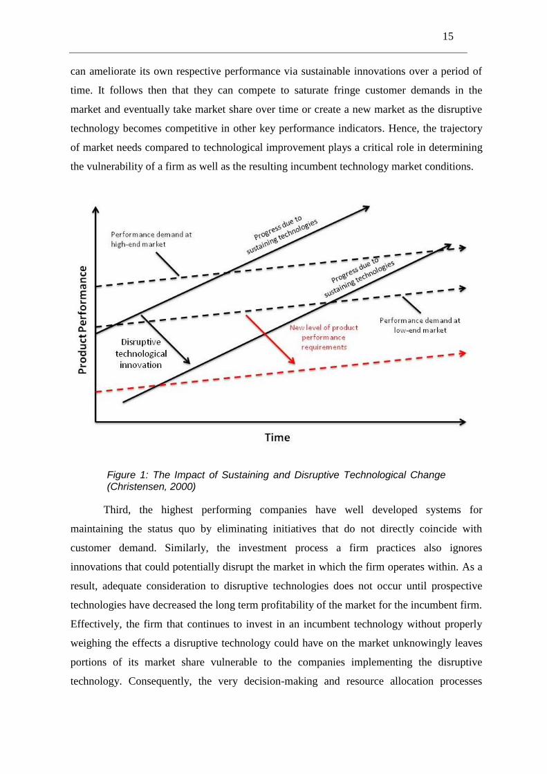
15

can ameliorate its own respective performance via sustainable innovations over a period of

time. It follows then that they can compete to saturate fringe customer demands in the

market and eventually take market share over time or create a new market as the disruptive

technology becomes competitive in other key performance indicators. Hence, the trajectory

of market needs compared to technological improvement plays a critical role in determining

the vulnerability of a firm as well as the resulting incumbent technology market conditions.

Figure 1: The Impact of Sustaining and Disruptive Technological Change (Christensen, 2000)

Third, the highest performing companies have well developed systems for

maintaining the status quo by eliminating initiatives that do not directly coincide with

customer demand. Similarly, the investment process a firm practices also ignores

innovations that could potentially disrupt the market in which the firm operates within. As a

result, adequate consideration to disruptive technologies does not occur until prospective

technologies have decreased the long term profitability of the market for the incumbent firm.

Effectively, the firm that continues to invest in an incumbent technology without properly

weighing the effects a disruptive technology could have on the market unknowingly leaves

portions of its market share vulnerable to the companies implementing the disruptive

technology. Consequently, the very decision-making and resource allocation processes

16

practiced by management, key to the success of well-established companies, are the very

processes that act as the root cause of their demise in the face of technological uncertainty.

Hence, these findings illustrate the unabating effects a disruptive technology has on

both a firm and an incumbent technology market. By not preparing for the potential change

in market conditions and lacking effective business action, a firm could lose its position in

the market as a result of not having the ability to properly weigh the aforementioned

elements and, consequently, risk failure. Hence, as good management practice drives the

failure of successful firms faced with disruptive technological change, then the conventional

responses to companies’ problems-planning better, working harder, becoming more

customer-driven, and taking a longer-term perspective- all exacerbate the problem. As such,

the solution to disruptive technologies lies within the laws of organizational nature which act

to powerfully define what a firm can and cannot do (Christensen, 2000).

3.2 Laws of Disruptive Technology

It is proposed by Christensen that there are five organizational laws of disruptive

technology that if properly harnessed lead to the success of a firm. In particular, the first and

third law provide useful properties that a firm can effectively leverage in order to decide

whether to invest in an incumbent technology given technological uncertainty or to divest

into a disruptive technology. First off, the primary law indicates that a firm depends on its

customers and investors for resources, whereas the third law stipulates that markets that do

not exist cannot be analyzed. By critically examining these two laws, it provides not only

grounded business action for a firm operating under technological uncertainty, but also gives

a basis for implicitly defining an investment model using regime-switching.

First, the theory of resource dependence governs a firm’s resource allocation. This

principle dictates that the firm does not control its own flow of resources, but, rather,

investors and customers are the forces within an organization that govern resource

allocation, and firms that choose to digress from satiating these needs ultimately fail.

Conversely, those that best satiate these needs are successful. As investment patterns are

designed to dismiss a disruptive technology at its outset, the only instance in which

mainstream firms have successfully established a timely position in a disruptive technology

were those in which the firm’s managers set up an autonomous organization charged with

building an independent business around the disruptive technology (Christensen, 2000).

17

Therefore, the companies that can best succeed in these small, emerging markets are those

that align their firms with forces of resource dependence by creating an independent

organization.

Secondly, the third law of disruptive technology stems from the innovator’s dilemma.

As the strategies to manage a sustainable technology are generally predictable, the strategies

are similarly competitively unimportant, whereas the leadership involved in fostering a

disruptive innovation displays large, advantageous aspects. However, companies whose

investment processes demand quantification of market sizes and financial returns before they

can enter a market become paralyzed or make serious mistakes when faced with disruptive

technologies (Christensen, 2000). As there are large first mover advantages in disruptive

situations, leadership must take action before careful plans can be made. However, as this

presents the innovator’s dilemma, it becomes necessary to recognize the unpredictability of a

new market. In order to overcome this aspect of innovation, Christensen suggests discovery-

driven planning. Due to the fact that very little is known about disruptive markets, effective

grounded business action is only applicable once a firm learns how best to implement a

disruptive technology. Hence, in planning to learn, the mindset needed for the exploitation of

a disruptive technology can be deduced after obtaining the necessary decision support

information to resolve underlying technological uncertainty.

In tying these two laws of disruptive technology together as well as the theory of

disruptive technology, regime-switching is implemented into the model due to its ability to

incorporate the hypothesized effects from a disruptive technology into incumbent technology

market conditions, as well as by providing a basis for responsive business action. By

incorporating regime-switching into the real options model, a change in incumbent

technology market conditions can implicitly reflect the hypothesized effects from the

successful penetration of a disruptive technology in the market. Additionally, grounded

business action can effectively be recommended based on the first and third organizational

laws of disruptive technology. In response to these laws, the firm no longer must base its

investment decision on a disruptive technology market but rather, implicitly on an incumbent

technology market, which gives the possibility to use market information from an observable

market instead of attempting to quantify the market size and financial return of a disruptive

market. Additionally, in the case that the option to invest is out of the money, the strategic

recommendations of either discovery-driven planning or, in the case of a successful venture,

the creation of a separate enterprise can be given. In conclusion, both the effects of

18

disruptive technology on incumbent technology market conditions and managerial insight

can be provided through the use of regime-switching in the proposed real options model.

19

4. Mathematical Background

4.1 Itô’s Lemma

Suppose the state variable follows a simple Brownian motion as indicated in Equation

(1). and are known, non-random functions, and is the standard increment

of a Wiener process.

(1)

Also, consider a function that is twice differentiable on and to the first-order

on the time variable . Through conventional calculus, the total differential of the function

can be expressed as Equation (2).

(2)

Introducing the higher-order terms of by Taylor expansion, the differential expands to

Equation (3).

(3)

In order to simplify Equation (3), the squared differential of the state variable is first

examined. Because the expected squared value of the Wiener increment is equal to the time

derivative, , taking the expansion of simplifies substantially as indicated in

(4). Empirically, it is observed that as becomes infinitesimally small, the first and second

term of the third line of (4) approach zero at a more rapid rate relative to . Hence, the

differentials of time with a power greater than one can be ignored.

(4)

20

Applying this same logic to any expansion of greater than the squared differential of

in Equation (3) will generate an expression with each time differentials’ exponent greater

than one and, hence, also cancel. Therefore, Equation (3) simplifies to Equation (5).

(5)

Collecting like terms, Itô’s Lemma gives the total differential of the function

generally as in Equation (6).

(6)

4.2 Markov-Modulated Geometric Brownian Motion

A stochastic variable is modelled by geometric Brownian motion with drift if it is a

specialized case of a continuous time stochastic process, , which, indicated in Equation

(7), can be found by adapting Equation (1) with and . This Itô

process has four distinct components where is an infinitesimally small increment of time,

is an increment of the standard Brownian motion, and and are the expected

instantaneous drift rate and the instantaneous variance rate respectively (Dixit and Pindyck,

1994).

(7)

As changes in the process over any finite interval of time are normally distributed, it

becomes necessary to transform the underlying function so that it can be used to suitably

model price. To do so, the relationship between the state variable and its logarithm is

examined, . Using Itô’s Lemma, its rate of change, can be expanded

resulting in Equation (8).

(8)

21

By inserting Equation (7) into Equation (8), the process followed by becomes described as

Equation (9). Hence, a change in a finite time interval in is normally distributed with a

mean and variance,

(9)

This result can be used to find both the expected value and variance of with its current,

observable state, , as indicated in (10).

(10)

Similarly, as this allows both the mean and variance of to be found, it enables the

expected present discounted value of to be calculated over a period of time by using the

result from (10) in Equation (11). In the case of perpetuity and an exogenous discount rate

where the discount rate exceeds the growth rate , the expectation provides a useful

outcome for the valuation of an investment project integrated under a perpetual time frame.

(11)

Secondly, as both the instantaneous drift and variance rate of geometric Brownian

motion fail to capture the effect disruptive technologies are hypothesized to have on

incumbent technology market conditions, the regime-switching model is introduced into

geometric Brownian motion parameters to capture these effects. In itself, regime-switching

often portrays the tendency financial markets have to exhibit volatile behaviour with the

phenomenon that the new behaviour often persists for several periods after such a change has

occurred. However, a key difference within this type of modelling occurs when looking at a

regime-switch that can be classified as either irreversible or highly unlikely to reoccur. These

changes, referred to as a change point process, were considered by Chib (1998) and further

expounded upon through the examination of stock return dynamics by Pástor and Stambaugh

(2001) and Pettenuzzo et al. (2014), amongst others. Within these processes, the

characteristics captured by these specific regime-switching models aim to correspond with

different periods in regulation, policy, and technological change (Ang and Timmermann,

2012). Logically, it follows that to document the effect a disruptive technological change has

22

on incumbent technology market conditions, regime-switching should be implemented in its

stochastic process.

In regime-switching models, there is an unobservable random state variable

that follows a Markov chain in the price process’s time series, that indicates which

regime, is realized in the economy. In a change point process, the regimes are no longer

revisited after a state change has occurred, and can theoretically be considered as sustainable

increments in disruptive technological change; with each subsequent regime visited, the

disruptive technology has implicitly made an incremental, but significant change that is

reflected in the incumbent technology’s market conditions.

Mathematically, this state change can be modelled by a modified transition

probability matrix where the probability of returning to a previous regime is zero. More

specifically, the regime-switch in a change point process is governed by a transition

probability matrix with the probabilities of switching from a regime at time to a

regime at time , as represented by the matrix in (12).

(12)

Additionally, the sum of the probabilities of switching to a particular regime or staying

within the realized regime sum to one for each respective regime as indicated in (13).

(13)

Moreover, each regime is assumed to be an independent price process that is

governed by the strong Markov property; the current regime is dependent upon only the

most recent realized regime , which corresponds to the transition probability matrix by the

probability as indicated in (14).

(14)

Practically, this implies that the point in time in which the process is applied is dependent

upon only current available information. Then, it follows that when applied to a current state,

the transition probability matrix is flexible in the sense that it can be applied at each step of

23

the Markov chain regardless of the state of the disruptive technology or the incumbent

technology market conditions. Hence, given these characteristics and the hypothesized

switching probabilities, a regime-switching valuation can effectively capture technological

uncertainty.

In addition, the change point process requires the probabilities , which can be

modelled using a Poisson jump process as denoted by in (15). This diffusion process

aims to model an economic variable as a process that makes infrequent but discrete jumps.

Consequently, the referenced jumps can be thought of as a substantial disruptive

technological breakthrough that causes the market conditions for the incumbent technology

to shift. Statistically, the Poisson jump process is subject to jumps of fixed or random size,

for which the arrival times follow a Poisson distribution (Dixit and Pindyck, 1994). The

jumps, , represent events that can cause a structural break in the stochastic process being

modelled, and which can in itself also be a random variable. The rate of occurrence or

intensity of the Poisson process is reflected by the proportionality constant λ, and during a

time interval of infinitesimal length , the probability that a jump will occur is given by

.

(15)

Finally, marrying these concepts together: geometric Brownian motion, regime-

switching, and a Poisson jump process; the state variable following Markov-modulated

geometric Brownian motion is described in Equation (16).

(16)

With the assumption that a Poisson jump process is modelled in the transition

probability matrix (17).

(17)

Consequently, the growth rate and volatility are subject to the realized regime in the

economy as indicated in (18).

24

(18)

By modelling the price process as such, Markov-modulated geometric Brownian motion can

implicitly incorporate relevant information about a disruptive technology in incumbent

technology market conditions to provide a more informed, capacity investment decision.

4.3 Dynamic Programming

Dynamic programming is a general tool used for dynamic optimization problems

under uncertainty. It decomposes a sequence of decisions into two components: the

immediate decision, and a valuation function that encapsulates the consequences of all

subsequent decisions (Dixit and Pindyck, 1994). This decomposition can be formally

described by Bellman’s Principle of Optimality,

“An optimal policy has the property that, whatever the initial action, the remaining

choices constitute an optimal policy with respect to the sub-problem starting at the state that

results from the initial actions” (Bellman, 1954).

In order to clarify these assertions, the components of a dynamic optimization

problem will be further analyzed in this section.

As indicated in Equation (19), during each period , a maximization choice is

represented by the control variable(s) , which denotes the specific choices to be made by

the firm. The firm’s current status as it affects its operations and expansion opportunities is

delineated by a state variable . Both of these variables at time affect the firm’s immediate

profit flow component, which can be denoted as As the valuation function is

evaluated from the perspective in period the expectation of the continuation value is taken,

, and further discounted to adjust to time by the discount factor

.

(19)

If there is no fixed finite time horizon for the decision problem, the dynamic optimization

problem becomes simplified in the sense that the calendar date ceases to have a direct

impact on the valuation. In this setting, the objective function gets a recursive structure that

25

facilitates theoretical analysis as well as numerical computation (Dixit and Pindyck, 1994) as

illustrated in Equation (20). In this situation, denotes the evaluation of the state in the next

period in relation to the current state

(20)

For a dynamic optimization problem in continuous time, the Bellman Equation (20) is

reworked to consider a time period of infinitesimal length in Equation (21).

(21)

By multiplying by a factor of , dividing by , and taking the limit as goes to

zero, Equation (21) becomes adapted for continuous time as indicated in Equation (22). In

real options terminology, this equation can be interpreted as the entitlement to the flow of

profits from an asset. In regards to the term, , the understanding behind this

component is the required rate of return a decision maker would demand from holding this

asset. The immediate profit flow component signifies the cash flow received upon

investment, which can be further considered the immediate payout or dividend of the asset.

Secondly, the continuation component can be interpreted as the expected rate of capital gain

on the asset.

(22)

To exemplify particular nuances of the solution of Equation (22), the optimization problem

is simplified so that the option can be modelled excluding its immediate payout as in

Equation (23). Additionally, for this purpose, it is assumed that the state variable follows a

geometric Brownian motion.

(23)

Using Itô’s Lemma, the right hand side of Equation (23) can be expanded with respect to the

underlying stochastic component of the asset, and, after simplification and

rearrangement, results in the differential equation (24).

26

(24)

Additionally, the general solution of Equation (24) must adhere to three boundary

conditions as indicated in (25) (Dixit and Pindyck, 1994). The first condition stems from the

absorbing barrier of the stochastic process followed by the state variable . Intuitively, this

indicates that if the price process reaches zero, the option to invest will be of no value.

Secondly, the second branch of (25) is known as the value-matching condition, and indicates

the net value of the asset by subtracting a project’s expected, discounted costs, from its

expected, discounted revenues at the optimal investment threshold, . Lastly, the third

branch of (25) is the smooth-pasting condition, which guarantees that the derivatives of the

functions, and , meet tangentially at a certain threshold point.

(25)

Furthermore, in order to satisfy the first branch of (25), it is assumed that the general

solution takes the functional format , which is then substituted into Equation

(24). By doing so, Equation (24) reduces to the fundamental quadratic outlined in Equation

(26).

(26)

In order to find a solution to Equation (26), the quadratic formula is implemented to outline

both the positive and negative roots of the solution, and , indicated in the first and

second branch of (27) respectively.

(27)

It then follows that as the second-order, Cauchy-Euler differential equation (24) is linear in

its dependent variable and its derivatives, it has a general solutions that can be

expressed as a linear combination of any two independent solutions as in Equation (28)

27

(Dixit and Pindyck, 1994). The endogenous constants, and , remain undetermined,

whereas and represent the aforementioned positive and negative roots of the proposed

form of the solution. Notice as and the absorbing barrier , the second term

in Equation (28) goes to infinity as . Hence, the second endogenous constant is set

equal to zero, , to mitigate this effect.

(28)

Consequently, from these three boundary conditions and the proposed form of the solution,

one can find the optimal investment policy by deriving both the optimal investment

threshold and the value of the option to invest.

28

5. Analytical Formulations

5.1 Assumptions and Notations

Consider a situation in which a price-taking firm faces an investment decision in

production capacity. Prior to investment, the firm is assumed to be generating no cash flow.

It can be interpreted that the firm is considering investment in incumbent technology

capacity while simultaneously weighing the possibility that an existing disruptive technology

will potentially shift incumbent technology market conditions. As such, the dynamics of

demand shock are governed by a Markov regime-switching model. In this model, the

incumbent technology market has an exogenous output price denoted by the variable

where time, , is considered to be continuous. Specifically, the exogenous output price

follows a Markov-modulated geometric Brownian motion as described in (29).

(29)

In this stochastic differential equation, the incumbent technology’s growth rate is denoted by

its volatility is represented by , and is the increment of the standard Brownian

motion. Also, the firm implements a subjective discount rate, which is considered

constant, and, intuitively, it follows that The demand shift parameter,

governs the switch between two regimes with both known growth rates and

volatilities. As it is assumed that there are only two regimes in the economy, the state-

dependent growth rates and volatilities take the form:

Within these two states, a specific incumbent technology market is represented. In the first

regime, a booming incumbent technology market is assumed where the disruptive

technology has not yet satiated or taken market demand. In the second regime, the resulting

incumbent technology market models the demand shock a successful disruptive technology

paradigm shift incurs. Consequently, the exogenous output price parameters in the

incumbent technology market has both boom- and recession-like characteristics, which are

reflected in regime one and regime two, respectively. Hence, as uncertainty is negatively

related to economic conditions (Goto et al., 2012, Bloom, 2009), a larger growth rate is

29

assumed in the first regime, , and a larger volatility is assumed in the second

regime .

In addition, the process is assumed to follow a Poisson law such that is a

two-state Markov chain with the transition from regime one to regime two characterized by a

jump with intensity As such, the process has the transition matrix between time

and :

This indicates that during an infinitesimal time interval there is a probability that the

booming incumbent technology market, will shift to a recessive incumbent

technology market, Conversely, during the infinitesimal time interval , there is a

probability that a regime-switch will not occur, and the incumbent technology

market will continue in regime one.

Additionally, project scale is denoted by the state variable when the firm has

discretion over investment timing. However, when a firm exercises investment in a now-or-

never investment opportunity, the capacity state variable is denoted by . What is more,

optimality is assumed by lower-case notation: is the time at which the firm exercises

the option to invest, denotes the optimal investment threshold, and ( is the

corresponding optimal capacity. In terms of costs, the firm must consider both an operating

and an investment cost in order to effectively evaluate the investment opportunity. Over the

production facility’s lifetime, an operating cost component is assumed of the incumbent

technology that is denoted by the deterministic variable, Likewise, the fixed and

irrecoverable investment cost is considered linked to capacity as displayed in (30).

(30)

In Equation (30), and are regarded as constants whereas the parameter implies that the

project investment costs exhibit diseconomies of scale as capacity sizing increases. The

fundamental basis of this assumption is commonly seen in both the renewable energy

industry as well as in a monopsonistic buyer environment in which a firm contemplates

investment facing increasing prices due to increasing demand (Chronopoulos et al., 2015,

Bøckman et al., 2008).

30

Moreover, immediate investment into additional capacity is considered the

opportunity cost of foregoing investment into a risk-free asset with a constant rate of return,

. Therefore, the net value of the investment project, takes this into consideration

by aggregating the net present value of immediate investment, , the deterministic

operating cost component, , as well as the opportunity cost of investment, . In

the case that the firm chooses to delay investment into additional capacity, the firm then

holds the perpetual option, , to invest in an incumbent technology project. Moreover, it

is assumed that once exercise of the option has occurred, production starts instantaneously at

full capacity with no operational flexibility to respond to exogenous demand factors. This

assumption linked to production flexibility is referenced as the clearance assumption, and

empirical evidence supporting this claim can be found in numerous pieces of literature

(Chod and Rudi, 2005, Chronopoulos et al., 2015). For example, large integrated steel

facilities exemplify this condition due to cost barriers to exit the steel industry. Pressure to

cover fixed costs, the integrated steel industry’s continuous production technology, and the

high cost of shutting down furnaces reinforce the producer’s resolve to continue production

as normal. Hence, these obstacles induce integrated steelmakers to continue stable

production in the face of diminishing returns (Madar, 2009).

5.2 The Model

In this section, an analytical framework for an incumbent technology, production

capacity investment decision will be developed. In order to do so, the investment decision

will be modelled through backward induction as an optimal stopping problem where the

solution will be proposed through the usage of the Bellman equation, as well as the value-

matching and smooth-pasting conditions. Furthermore, analytical expressions governing the

value of the option to invest, the optimal investment threshold and the corresponding optimal

capacity under price and technological uncertainty will be derived. In order to account for

technological uncertainty, regime-switching will be incorporated into the model.

5.2.1 Regime 2

First off, an expression governing the firm’s optimization objective is derived as

indicated in (31). The inner maximization of (31) represents the net payout from immediate

investment in the project. As the output price, is fixed and known at the time of

31

investment, the analytical expression is maximized with respect to the capacity of the

project, . Furthermore, the left-hand side of the maximization represents the option to

invest. According to the Bellman principle, an investment opportunity over an infinitesimal

time interval, is the equivalent of the expected rate of capital appreciation of an asset

(Dixit and Pindyck, 1994), which is further interpreted according to the price process,

. By combining these two respective valuations together, the firm can then derive the

optimal stopping policy analogous to the same mechanism in which a financial call option is

exercised.

(31)

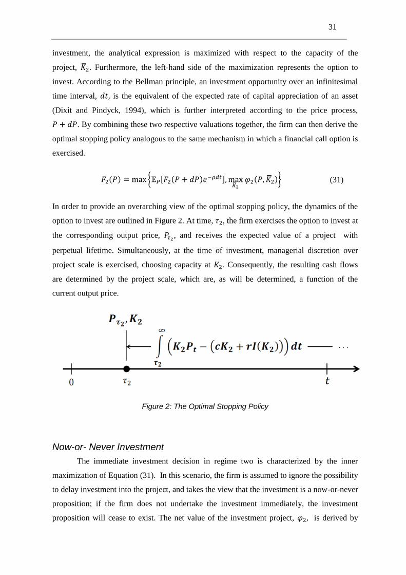
In order to provide an overarching view of the optimal stopping policy, the dynamics of the

option to invest are outlined in Figure 2. At time, , the firm exercises the option to invest at

the corresponding output price, , and receives the expected value of a project with

perpetual lifetime. Simultaneously, at the time of investment, managerial discretion over

project scale is exercised, choosing capacity at . Consequently, the resulting cash flows

are determined by the project scale, which are, as will be determined, a function of the

current output price.

Figure 2: The Optimal Stopping Policy

Now-or- Never Investment

The immediate investment decision in regime two is characterized by the inner

maximization of Equation (31). In this scenario, the firm is assumed to ignore the possibility

to delay investment into the project, and takes the view that the investment is a now-or-never

proposition; if the firm does not undertake the investment immediately, the investment

proposition will cease to exist. The net value of the investment project, is derived by

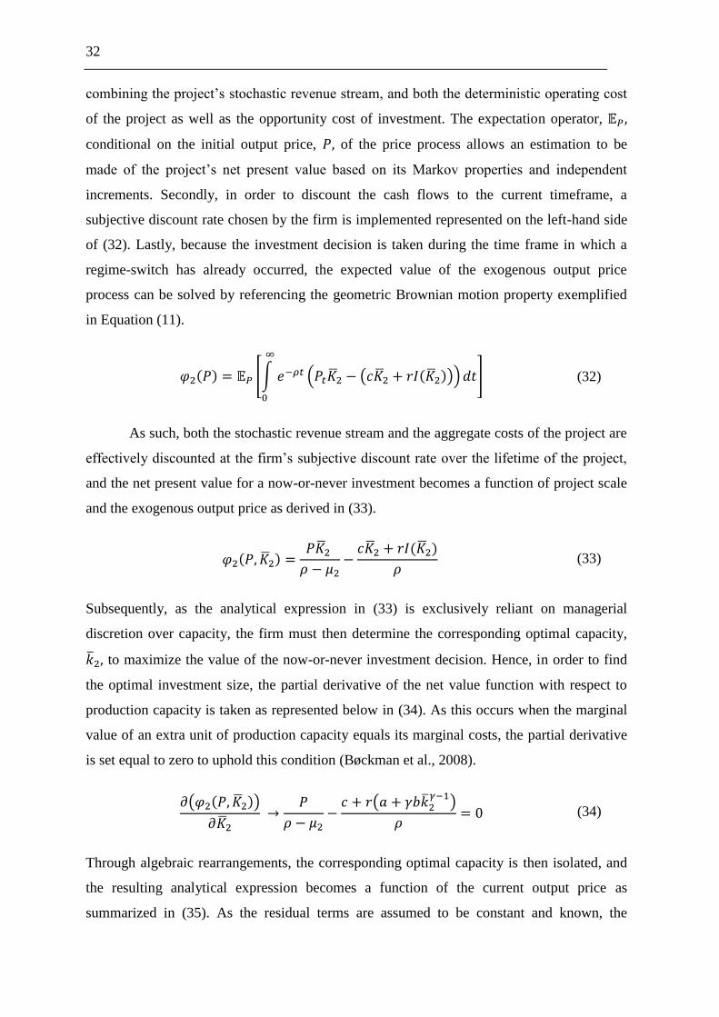
32

combining the project’s stochastic revenue stream, and both the deterministic operating cost

of the project as well as the opportunity cost of investment. The expectation operator,

conditional on the initial output price, of the price process allows an estimation to be

made of the project’s net present value based on its Markov properties and independent

increments. Secondly, in order to discount the cash flows to the current timeframe, a

subjective discount rate chosen by the firm is implemented represented on the left-hand side

of (32). Lastly, because the investment decision is taken during the time frame in which a

regime-switch has already occurred, the expected value of the exogenous output price

process can be solved by referencing the geometric Brownian motion property exemplified

in Equation (11).

(32)

As such, both the stochastic revenue stream and the aggregate costs of the project are

effectively discounted at the firm’s subjective discount rate over the lifetime of the project,

and the net present value for a now-or-never investment becomes a function of project scale

and the exogenous output price as derived in (33).

(33)

Subsequently, as the analytical expression in (33) is exclusively reliant on managerial

discretion over capacity, the firm must then determine the corresponding optimal capacity,

to maximize the value of the now-or-never investment decision. Hence, in order to find

the optimal investment size, the partial derivative of the net value function with respect to

production capacity is taken as represented below in (34). As this occurs when the marginal

value of an extra unit of production capacity equals its marginal costs, the partial derivative

is set equal to zero to uphold this condition (Bøckman et al., 2008).

(34)

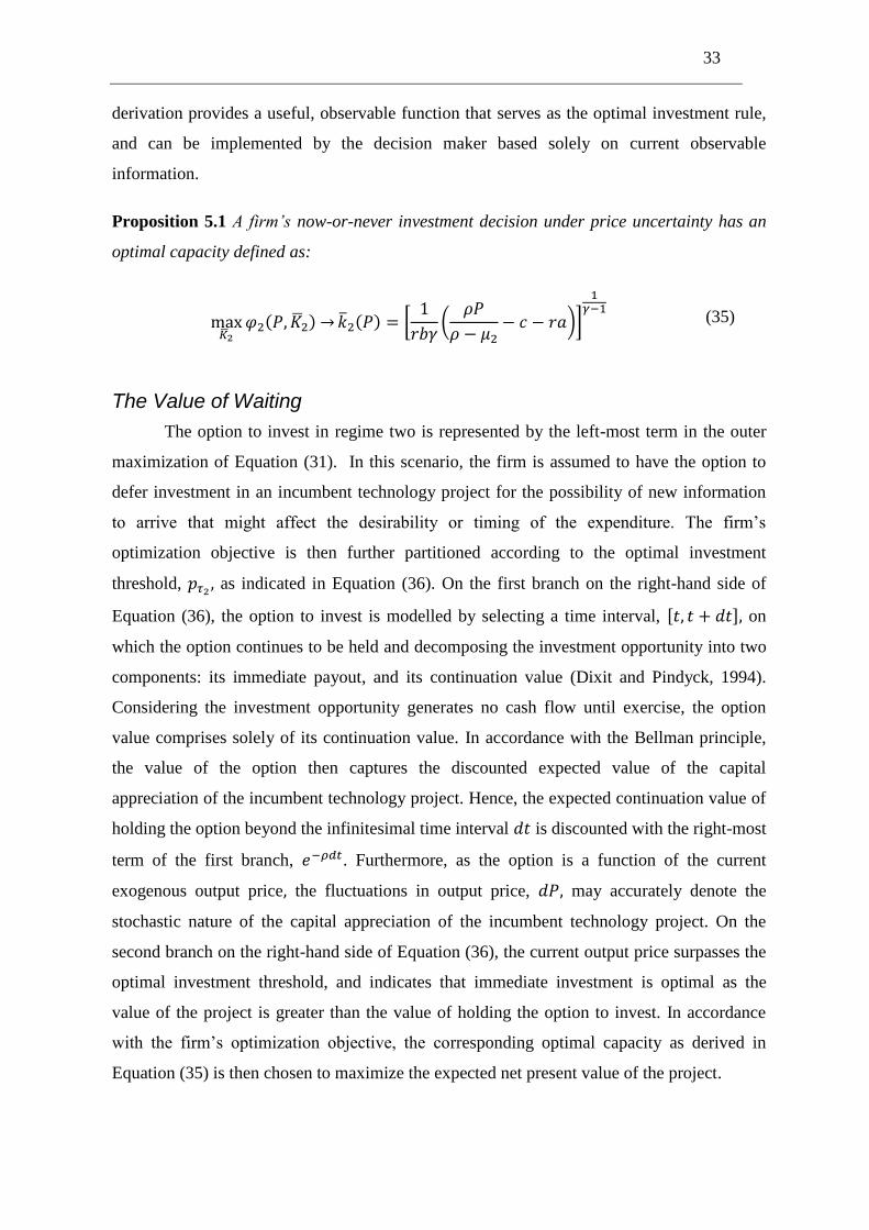
Through algebraic rearrangements, the corresponding optimal capacity is then isolated, and

the resulting analytical expression becomes a function of the current output price as

summarized in (35). As the residual terms are assumed to be constant and known, the

33

derivation provides a useful, observable function that serves as the optimal investment rule,

and can be implemented by the decision maker based solely on current observable

information.

Proposition 5.1 A firm’s now-or-never investment decision under price uncertainty has an

optimal capacity defined as:

(35)

The Value of Waiting

The option to invest in regime two is represented by the left-most term in the outer

maximization of Equation (31). In this scenario, the firm is assumed to have the option to

defer investment in an incumbent technology project for the possibility of new information

to arrive that might affect the desirability or timing of the expenditure. The firm’s

optimization objective is then further partitioned according to the optimal investment

threshold, as indicated in Equation (36). On the first branch on the right-hand side of

Equation (36), the option to invest is modelled by selecting a time interval, on

which the option continues to be held and decomposing the investment opportunity into two

components: its immediate payout, and its continuation value (Dixit and Pindyck, 1994).

Considering the investment opportunity generates no cash flow until exercise, the option

value comprises solely of its continuation value. In accordance with the Bellman principle,

the value of the option then captures the discounted expected value of the capital

appreciation of the incumbent technology project. Hence, the expected continuation value of

holding the option beyond the infinitesimal time interval is discounted with the right-most

term of the first branch, . Furthermore, as the option is a function of the current

exogenous output price the fluctuations in output price, may accurately denote the

stochastic nature of the capital appreciation of the incumbent technology project. On the

second branch on the right-hand side of Equation (36), the current output price surpasses the

optimal investment threshold, and indicates that immediate investment is optimal as the

value of the project is greater than the value of holding the option to invest. In accordance

with the firm’s optimization objective, the corresponding optimal capacity as derived in

Equation (35) is then chosen to maximize the expected net present value of the project.

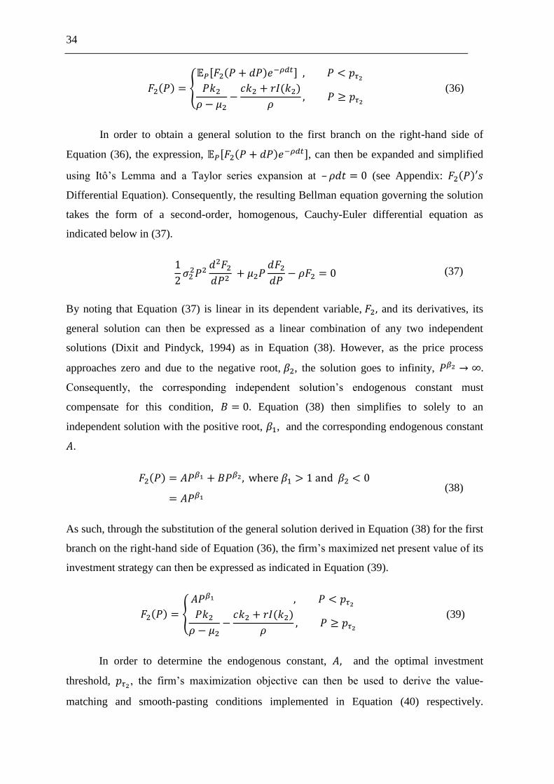
34

(36)

In order to obtain a general solution to the first branch on the right-hand side of

Equation (36), the expression, , can then be expanded and simplified

using Itô’s Lemma and a Taylor series expansion at – (see Appendix:

Differential Equation). Consequently, the resulting Bellman equation governing the solution

takes the form of a second-order, homogenous, Cauchy-Euler differential equation as

indicated below in (37).

(37)

By noting that Equation (37) is linear in its dependent variable, and its derivatives, its

general solution can then be expressed as a linear combination of any two independent

solutions (Dixit and Pindyck, 1994) as in Equation (38). However, as the price process

approaches zero and due to the negative root, , the solution goes to infinity,

Consequently, the corresponding independent solution’s endogenous constant must

compensate for this condition, Equation (38) then simplifies to solely to an

independent solution with the positive root, , and the corresponding endogenous constant

.

(38)

As such, through the substitution of the general solution derived in Equation (38) for the first

branch on the right-hand side of Equation (36), the firm’s maximized net present value of its

investment strategy can then be expressed as indicated in Equation (39).

(39)

In order to determine the endogenous constant, and the optimal investment

threshold, , the firm’s maximization objective can then be used to derive the value-

matching and smooth-pasting conditions implemented in Equation (40) respectively.

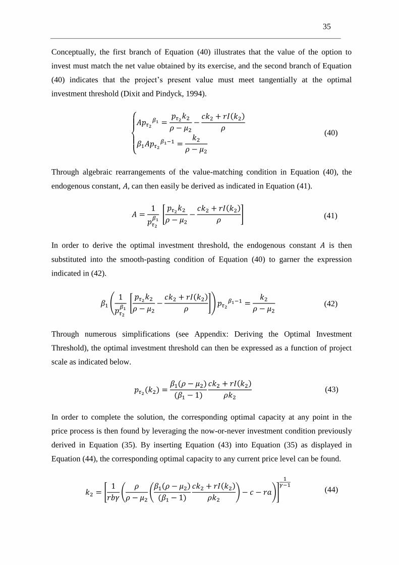
35

Conceptually, the first branch of Equation (40) illustrates that the value of the option to

invest must match the net value obtained by its exercise, and the second branch of Equation

(40) indicates that the project’s present value must meet tangentially at the optimal

investment threshold (Dixit and Pindyck, 1994).

(40)

Through algebraic rearrangements of the value-matching condition in Equation (40), the

endogenous constant, can then easily be derived as indicated in Equation (41).

(41)

In order to derive the optimal investment threshold, the endogenous constant is then

substituted into the smooth-pasting condition of Equation (40) to garner the expression

indicated in (42).

(42)

Through numerous simplifications (see Appendix: Deriving the Optimal Investment

Threshold), the optimal investment threshold can then be expressed as a function of project

scale as indicated below.

(43)

In order to complete the solution, the corresponding optimal capacity at any point in the

price process is then found by leveraging the now-or-never investment condition previously

derived in Equation (35). By inserting Equation (43) into Equation (35) as displayed in

Equation (44), the corresponding optimal capacity to any current price level can be found.

(44)

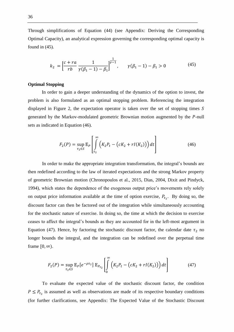
36

Through simplifications of Equation (44) (see Appendix: Deriving the Corresponding

Optimal Capacity), an analytical expression governing the corresponding optimal capacity is

found in (45).

(45)

Optimal Stopping

In order to gain a deeper understanding of the dynamics of the option to invest, the

problem is also formulated as an optimal stopping problem. Referencing the integration

displayed in Figure 2, the expectation operator is taken over the set of stopping times

generated by the Markov-modulated geometric Brownian motion augmented by the -null

sets as indicated in Equation (46).

(46)

In order to make the appropriate integration transformation, the integral’s bounds are

then redefined according to the law of iterated expectations and the strong Markov property

of geometric Brownian motion (Chronopoulos et al., 2015, Dias, 2004, Dixit and Pindyck,

1994), which states the dependence of the exogenous output price’s movements rely solely

on output price information available at the time of option exercise, . By doing so, the

discount factor can then be factored out of the integration while simultaneously accounting

for the stochastic nature of exercise. In doing so, the time at which the decision to exercise

ceases to affect the integral’s bounds as they are accounted for in the left-most argument in

Equation (47). Hence, by factoring the stochastic discount factor, the calendar date no

longer bounds the integral, and the integration can be redefined over the perpetual time

frame .

(47)

To evaluate the expected value of the stochastic discount factor, the condition

is assumed as well as observations are made of its respective boundary conditions

(for further clarifications, see Appendix: The Expected Value of the Stochastic Discount

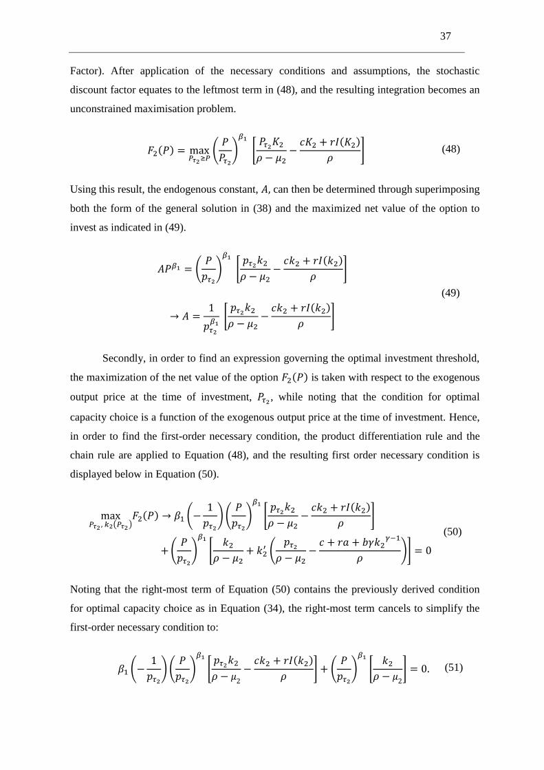
37

Factor). After application of the necessary conditions and assumptions, the stochastic

discount factor equates to the leftmost term in (48), and the resulting integration becomes an

unconstrained maximisation problem.

(48)

Using this result, the endogenous constant, can then be determined through superimposing

both the form of the general solution in (38) and the maximized net value of the option to

invest as indicated in (49).

(49)

Secondly, in order to find an expression governing the optimal investment threshold,

the maximization of the net value of the option is taken with respect to the exogenous

output price at the time of investment, , while noting that the condition for optimal

capacity choice is a function of the exogenous output price at the time of investment. Hence,

in order to find the first-order necessary condition, the product differentiation rule and the

chain rule are applied to Equation (48), and the resulting first order necessary condition is

displayed below in Equation (50).

(50)

Noting that the right-most term of Equation (50) contains the previously derived condition

for optimal capacity choice as in Equation (34), the right-most term cancels to simplify the

first-order necessary condition to:

(51)

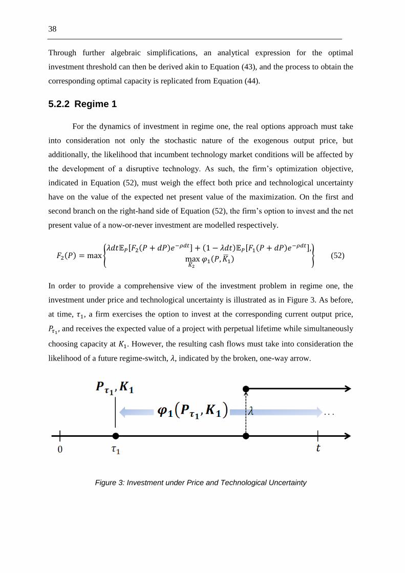
38

Through further algebraic simplifications, an analytical expression for the optimal

investment threshold can then be derived akin to Equation (43), and the process to obtain the

corresponding optimal capacity is replicated from Equation (44).

5.2.2 Regime 1

For the dynamics of investment in regime one, the real options approach must take

into consideration not only the stochastic nature of the exogenous output price, but

additionally, the likelihood that incumbent technology market conditions will be affected by

the development of a disruptive technology. As such, the firm’s optimization objective,

indicated in Equation (52), must weigh the effect both price and technological uncertainty

have on the value of the expected net present value of the maximization. On the first and

second branch on the right-hand side of Equation (52), the firm’s option to invest and the net

present value of a now-or-never investment are modelled respectively.

(52)

In order to provide a comprehensive view of the investment problem in regime one, the

investment under price and technological uncertainty is illustrated as in Figure 3. As before,

at time, , a firm exercises the option to invest at the corresponding current output price,

and receives the expected value of a project with perpetual lifetime while simultaneously

choosing capacity at . However, the resulting cash flows must take into consideration the

likelihood of a future regime-switch, , indicated by the broken, one-way arrow.

Figure 3: Investment under Price and Technological Uncertainty

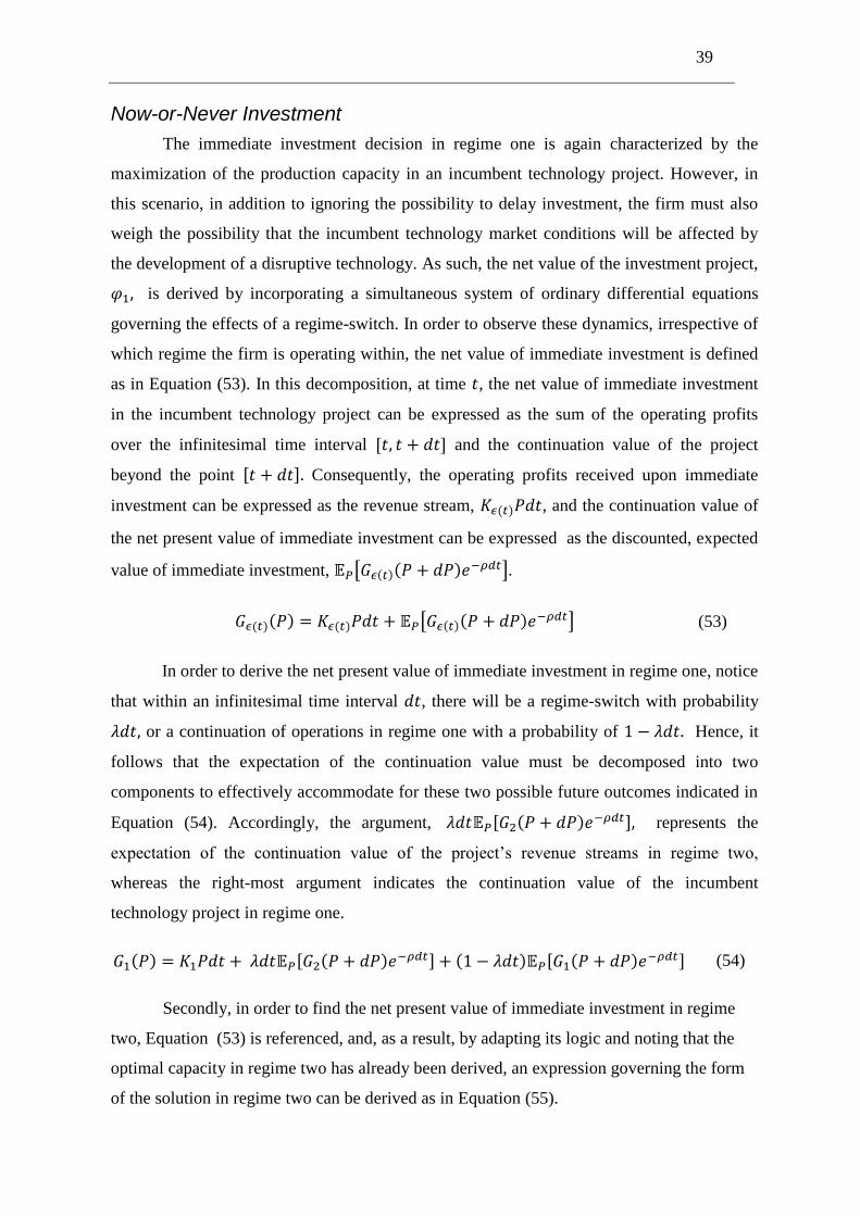
39

Now-or-Never Investment

The immediate investment decision in regime one is again characterized by the

maximization of the production capacity in an incumbent technology project. However, in

this scenario, in addition to ignoring the possibility to delay investment, the firm must also

weigh the possibility that the incumbent technology market conditions will be affected by

the development of a disruptive technology. As such, the net value of the investment project,

is derived by incorporating a simultaneous system of ordinary differential equations

governing the effects of a regime-switch. In order to observe these dynamics, irrespective of

which regime the firm is operating within, the net value of immediate investment is defined

as in Equation (53). In this decomposition, at time , the net value of immediate investment

in the incumbent technology project can be expressed as the sum of the operating profits

over the infinitesimal time interval and the continuation value of the project

beyond the point Consequently, the operating profits received upon immediate

investment can be expressed as the revenue stream, , and the continuation value of

the net present value of immediate investment can be expressed as the discounted, expected

value of immediate investment,

(53)

In order to derive the net present value of immediate investment in regime one, notice

that within an infinitesimal time interval , there will be a regime-switch with probability

or a continuation of operations in regime one with a probability of Hence, it

follows that the expectation of the continuation value must be decomposed into two

components to effectively accommodate for these two possible future outcomes indicated in

Equation (54). Accordingly, the argument, represents the

expectation of the continuation value of the project’s revenue streams in regime two,

whereas the right-most argument indicates the continuation value of the incumbent

technology project in regime one.

(54)

Secondly, in order to find the net present value of immediate investment in regime

two, Equation (53) is referenced, and, as a result, by adapting its logic and noting that the

optimal capacity in regime two has already been derived, an expression governing the form

of the solution in regime two can be derived as in Equation (55).

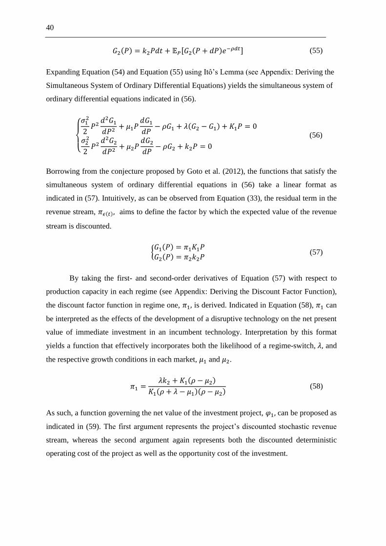
40

(55)

Expanding Equation (54) and Equation (55) using Itô’s Lemma (see Appendix: Deriving the

Simultaneous System of Ordinary Differential Equations) yields the simultaneous system of

ordinary differential equations indicated in (56).

(56)

Borrowing from the conjecture proposed by Goto et al. (2012), the functions that satisfy the

simultaneous system of ordinary differential equations in (56) take a linear format as

indicated in (57). Intuitively, as can be observed from Equation (33), the residual term in the

revenue stream, aims to define the factor by which the expected value of the revenue

stream is discounted.

(57)

By taking the first- and second-order derivatives of Equation (57) with respect to

production capacity in each regime (see Appendix: Deriving the Discount Factor Function),

the discount factor function in regime one, is derived. Indicated in Equation (58), can

be interpreted as the effects of the development of a disruptive technology on the net present

value of immediate investment in an incumbent technology. Interpretation by this format

yields a function that effectively incorporates both the likelihood of a regime-switch, and

the respective growth conditions in each market, and .

(58)

As such, a function governing the net value of the investment project, can be proposed as

indicated in (59). The first argument represents the project’s discounted stochastic revenue

stream, whereas the second argument again represents both the discounted deterministic

operating cost of the project as well as the opportunity cost of the investment.

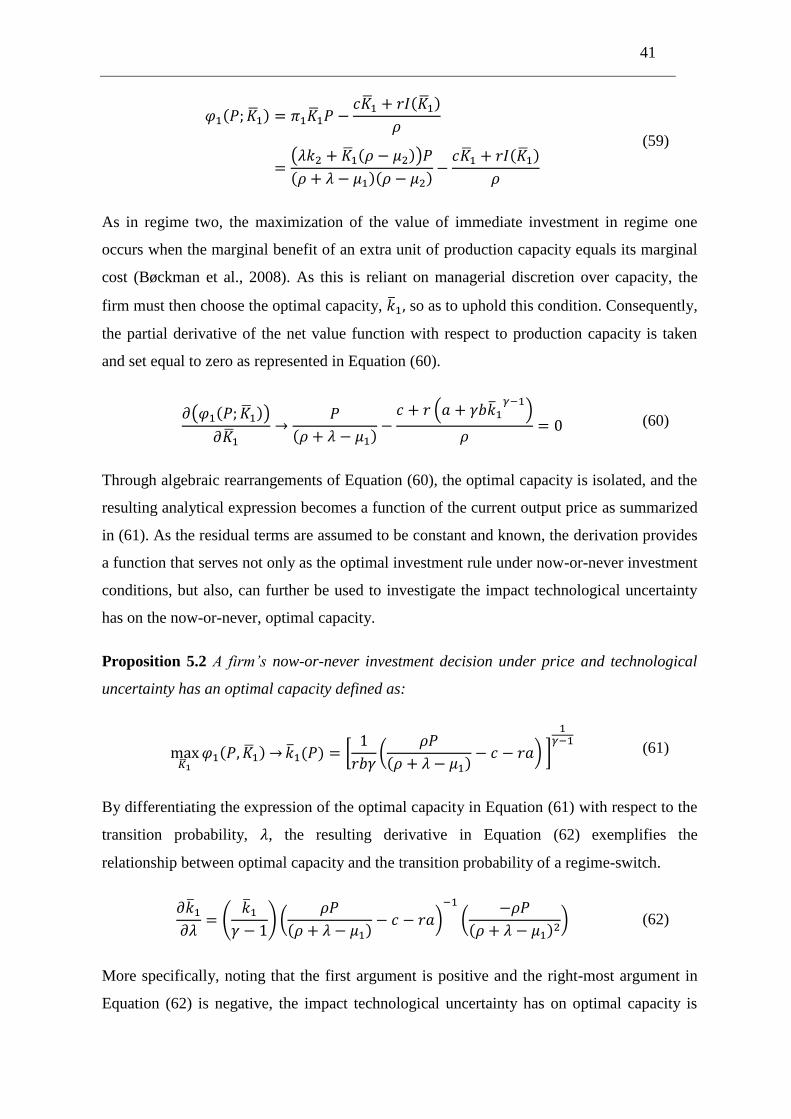
41

(59)

As in regime two, the maximization of the value of immediate investment in regime one

occurs when the marginal benefit of an extra unit of production capacity equals its marginal

cost (Bøckman et al., 2008). As this is reliant on managerial discretion over capacity, the

firm must then choose the optimal capacity, so as to uphold this condition. Consequently,

the partial derivative of the net value function with respect to production capacity is taken

and set equal to zero as represented in Equation (60).

(60)

Through algebraic rearrangements of Equation (60), the optimal capacity is isolated, and the

resulting analytical expression becomes a function of the current output price as summarized

in (61). As the residual terms are assumed to be constant and known, the derivation provides

a function that serves not only as the optimal investment rule under now-or-never investment

conditions, but also, can further be used to investigate the impact technological uncertainty

has on the now-or-never, optimal capacity.

Proposition 5.2 A firm’s now-or-never investment decision under price and technological

uncertainty has an optimal capacity defined as:

(61)

By differentiating the expression of the optimal capacity in Equation (61) with respect to the

transition probability, , the resulting derivative in Equation (62) exemplifies the

relationship between optimal capacity and the transition probability of a regime-switch.

(62)

More specifically, noting that the first argument is positive and the right-most argument in

Equation (62) is negative, the impact technological uncertainty has on optimal capacity is

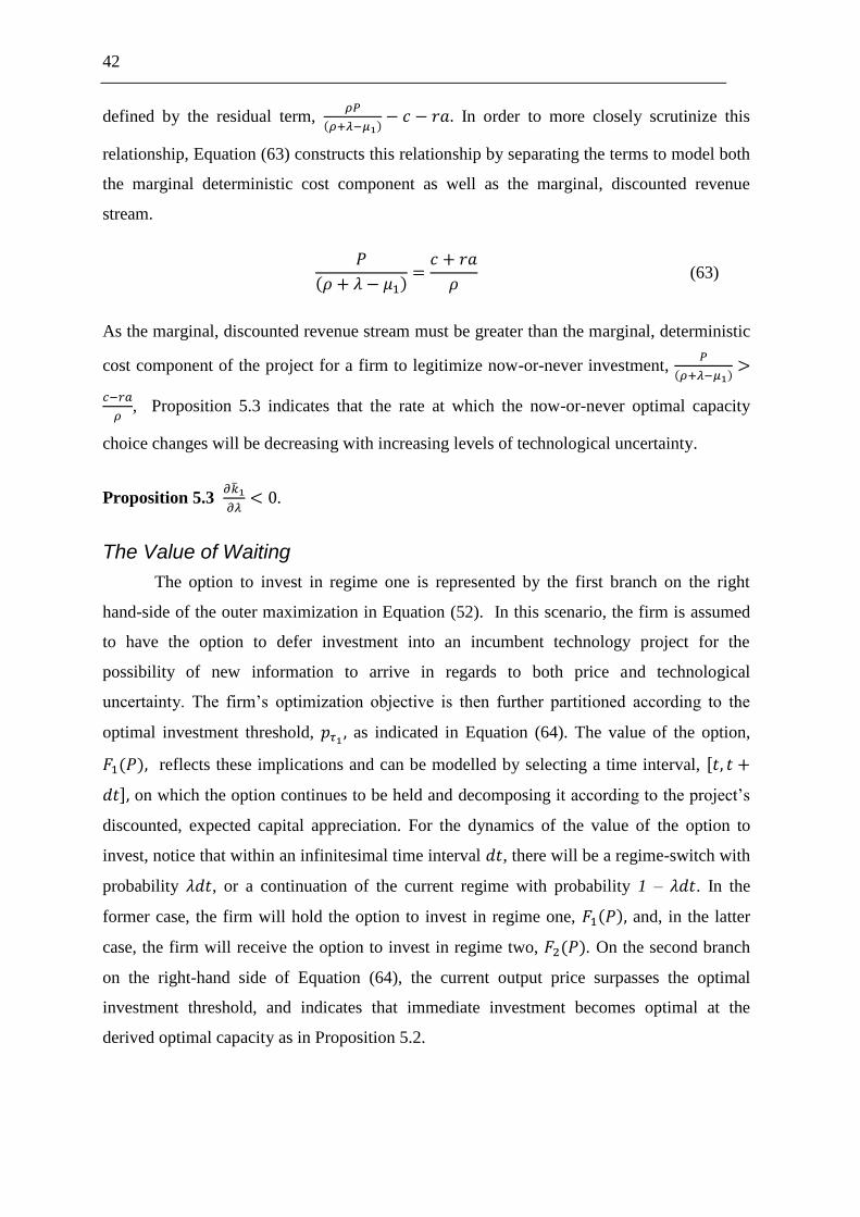
42

defined by the residual term,

In order to more closely scrutinize this

relationship, Equation (63) constructs this relationship by separating the terms to model both

the marginal deterministic cost component as well as the marginal, discounted revenue

stream.

(63)

As the marginal, discounted revenue stream must be greater than the marginal, deterministic

cost component of the project for a firm to legitimize now-or-never investment,

, Proposition 5.3 indicates that the rate at which the now-or-never optimal capacity

choice changes will be decreasing with increasing levels of technological uncertainty.

Proposition 5.3

.

The Value of Waiting

The option to invest in regime one is represented by the first branch on the right

hand-side of the outer maximization in Equation (52). In this scenario, the firm is assumed

to have the option to defer investment into an incumbent technology project for the

possibility of new information to arrive in regards to both price and technological

uncertainty. The firm’s optimization objective is then further partitioned according to the

optimal investment threshold, as indicated in Equation (64). The value of the option,

reflects these implications and can be modelled by selecting a time interval,

on which the option continues to be held and decomposing it according to the project’s

discounted, expected capital appreciation. For the dynamics of the value of the option to

invest, notice that within an infinitesimal time interval , there will be a regime-switch with

probability , or a continuation of the current regime with probability 1 – . In the

former case, the firm will hold the option to invest in regime one, and, in the latter

case, the firm will receive the option to invest in regime two, . On the second branch

on the right-hand side of Equation (64), the current output price surpasses the optimal

investment threshold, and indicates that immediate investment becomes optimal at the

derived optimal capacity as in Proposition 5.2.

43

(64)

Noting that has already been determined in the previous section, the differential

equation in (64) is expanded using both Itô’s Lemma and a Taylor series expansion at

– (see Appendix: Differential Equation), which results in (65).

Consequently, the resulting Bellman equation governing the solution takes the form of a

second-order, non-homogenous, Cauchy-Euler differential equation.

(65)

By noting that the differential equation in (65) must be solved for both its

homogenous and non-homogenous components, a general and a particular solution is

conjectured in Equation (66). From the fundamental quadratic equation, it is known that the

linear combination of independent solutions has both a positive and negative root, indicated

by , respectively. Hence, as aforementioned, the solution becomes

undefined as the exogenous output price approaches zero with regards to the independent

solution with the negative root. As a result, the endogenous component is set equal to zero

to circumvent this limitation, and, consequently, the term, drops out of the form of the

solution. Hence, the remaining linear, independent solution with a positive root, , where

is an endogenous coefficient, constitutes the homogenous component of the solution in

(66). Additionally, the non-homogenous component of the solution stems from the transition

probability of a regime-switch as indicated by the term, As the value of the option to

invest in regime two takes the analogous form of a call option, , it is proposed

using the method of undetermined coefficients that the non-homogenous component of the

solution takes the form .

(66)

Through the conjectured solution in (66), Equation (65) is manipulated to find an analytical

expression for the endogenous constant as indicated in Equation (67) (see Appendix:

Deriving the Endogenous Constant ).

44

(67)

As such, through the substitution of the solution derived in Equation (66) for the first branch

on the right-hand side of Equation (64), the firm’s maximized net present value of its

investment strategy can then be expressed as indicated in Equation (68).

(68)

Due to the mathematical limitations on nonlinear equations, the value-matching and

smooth-pasting conditions cannot be used to solve for an analytical solution. Instead, the

endogenous constant the optimal investment threshold and its corresponding optimal

capacity are determined through iterative, numeric methods using Matlab in the

following section.

However, theoretically, an encompassing investment strategy can be advised to the

firm facing an investment decision under price and technological uncertainty. First off, when

the current output price for an incumbent technology is below the optimal investment

threshold, the firm continues to hold the option as the value of the option surpasses the value

of immediate exercise. Simultaneously, holding the option to invest in an incumbent

technology is a precursor of discovery-driven planning as it implicitly warns the firm of the

incumbent technology’s potential demise. Hence, according to the first and third

organizational laws of disruptive technology, a firm contemplating investment into an

incumbent technology while holding the option to invest should weigh the strategic

implications of discovery-driven planning.

Remark 5.1 As long as the option to invest in an incumbent technology is held under

technological uncertainty, a firm should implement discovery-driven planning in disruptive

technology.

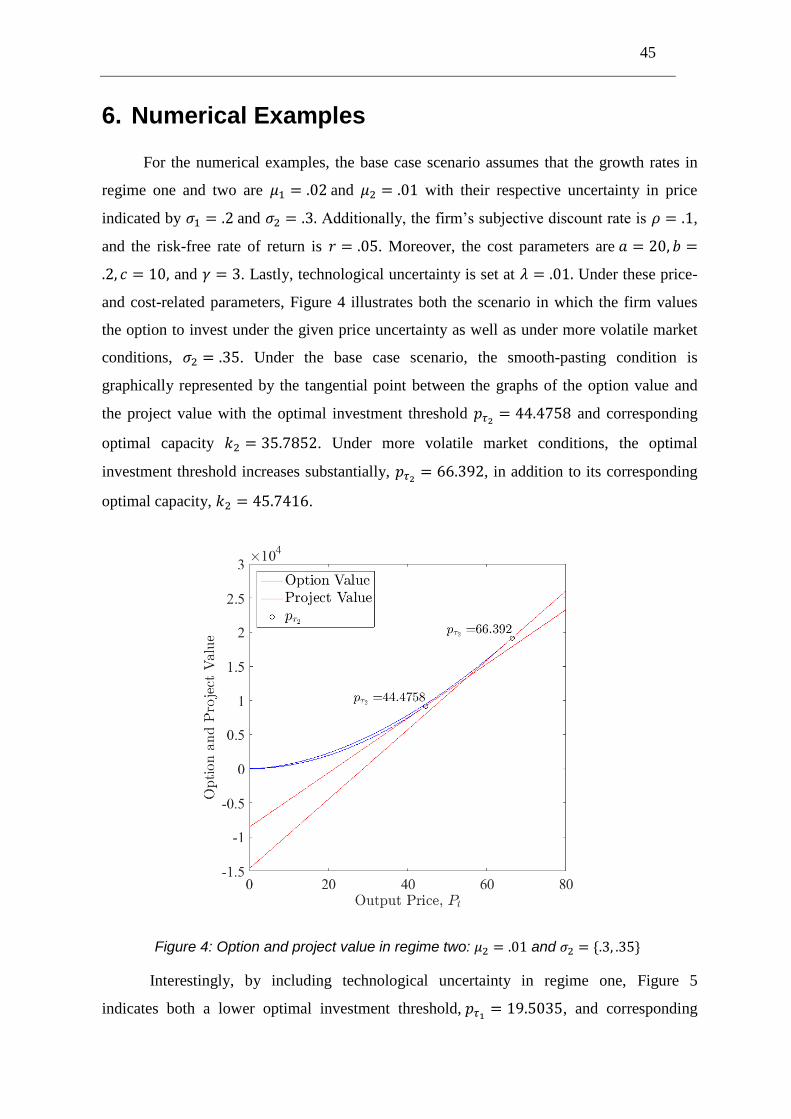
45

6. Numerical Examples

For the numerical examples, the base case scenario assumes that the growth rates in

regime one and two are and with their respective uncertainty in price

indicated by and Additionally, the firm’s subjective discount rate is ,

and the risk-free rate of return is . Moreover, the cost parameters are

and . Lastly, technological uncertainty is set at Under these price-

and cost-related parameters, Figure 4 illustrates both the scenario in which the firm values

the option to invest under the given price uncertainty as well as under more volatile market

conditions, . Under the base case scenario, the smooth-pasting condition is

graphically represented by the tangential point between the graphs of the option value and

the project value with the optimal investment threshold and corresponding

optimal capacity . Under more volatile market conditions, the optimal

investment threshold increases substantially, , in addition to its corresponding

optimal capacity, .

Figure 4: Option and project value in regime two: and

Interestingly, by including technological uncertainty in regime one, Figure 5

indicates both a lower optimal investment threshold, , and corresponding

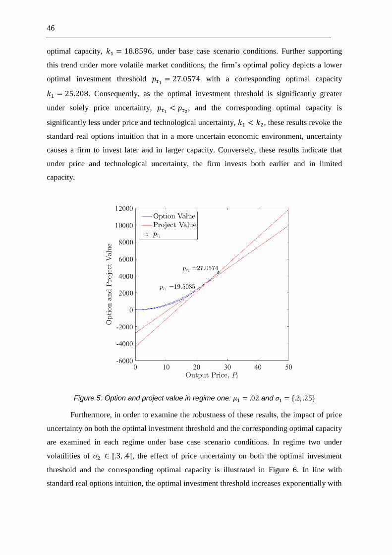
46

optimal capacity, , under base case scenario conditions. Further supporting

this trend under more volatile market conditions, the firm’s optimal policy depicts a lower

optimal investment threshold with a corresponding optimal capacity

. Consequently, as the optimal investment threshold is significantly greater

under solely price uncertainty, , and the corresponding optimal capacity is

significantly less under price and technological uncertainty, , these results revoke the

standard real options intuition that in a more uncertain economic environment, uncertainty

causes a firm to invest later and in larger capacity. Conversely, these results indicate that

under price and technological uncertainty, the firm invests both earlier and in limited

capacity.

Figure 5: Option and project value in regime one: and

Furthermore, in order to examine the robustness of these results, the impact of price

uncertainty on both the optimal investment threshold and the corresponding optimal capacity

are examined in each regime under base case scenario conditions. In regime two under

volatilities of , the effect of price uncertainty on both the optimal investment

threshold and the corresponding optimal capacity is illustrated in Figure 6. In line with

standard real options intuition, the optimal investment threshold increases exponentially with

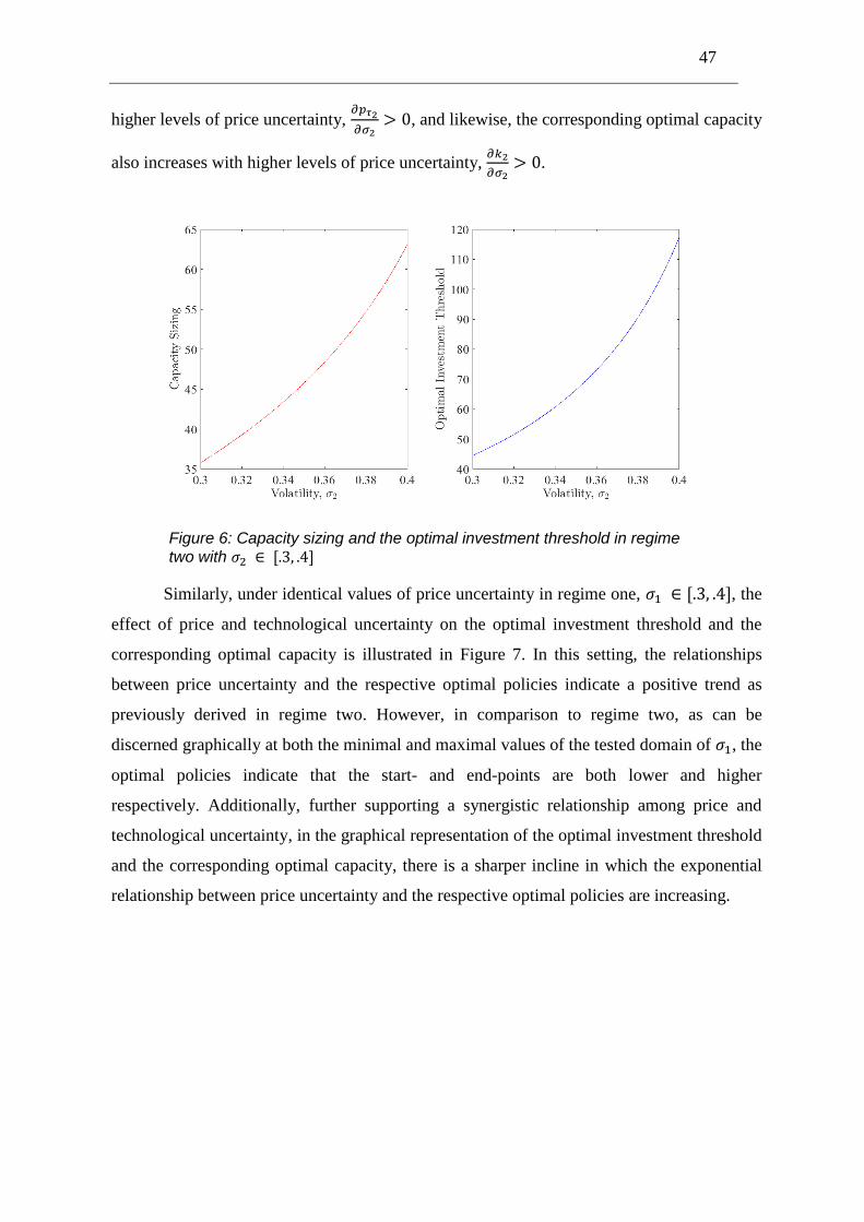
47

higher levels of price uncertainty,

, and likewise, the corresponding optimal capacity

also increases with higher levels of price uncertainty,

.

Figure 6: Capacity sizing and the optimal investment threshold in regime two with

Similarly, under identical values of price uncertainty in regime one, , the

effect of price and technological uncertainty on the optimal investment threshold and the

corresponding optimal capacity is illustrated in Figure 7. In this setting, the relationships

between price uncertainty and the respective optimal policies indicate a positive trend as

previously derived in regime two. However, in comparison to regime two, as can be

discerned graphically at both the minimal and maximal values of the tested domain of , the

optimal policies indicate that the start- and end-points are both lower and higher

respectively. Additionally, further supporting a synergistic relationship among price and

technological uncertainty, in the graphical representation of the optimal investment threshold

and the corresponding optimal capacity, there is a sharper incline in which the exponential

relationship between price uncertainty and the respective optimal policies are increasing.

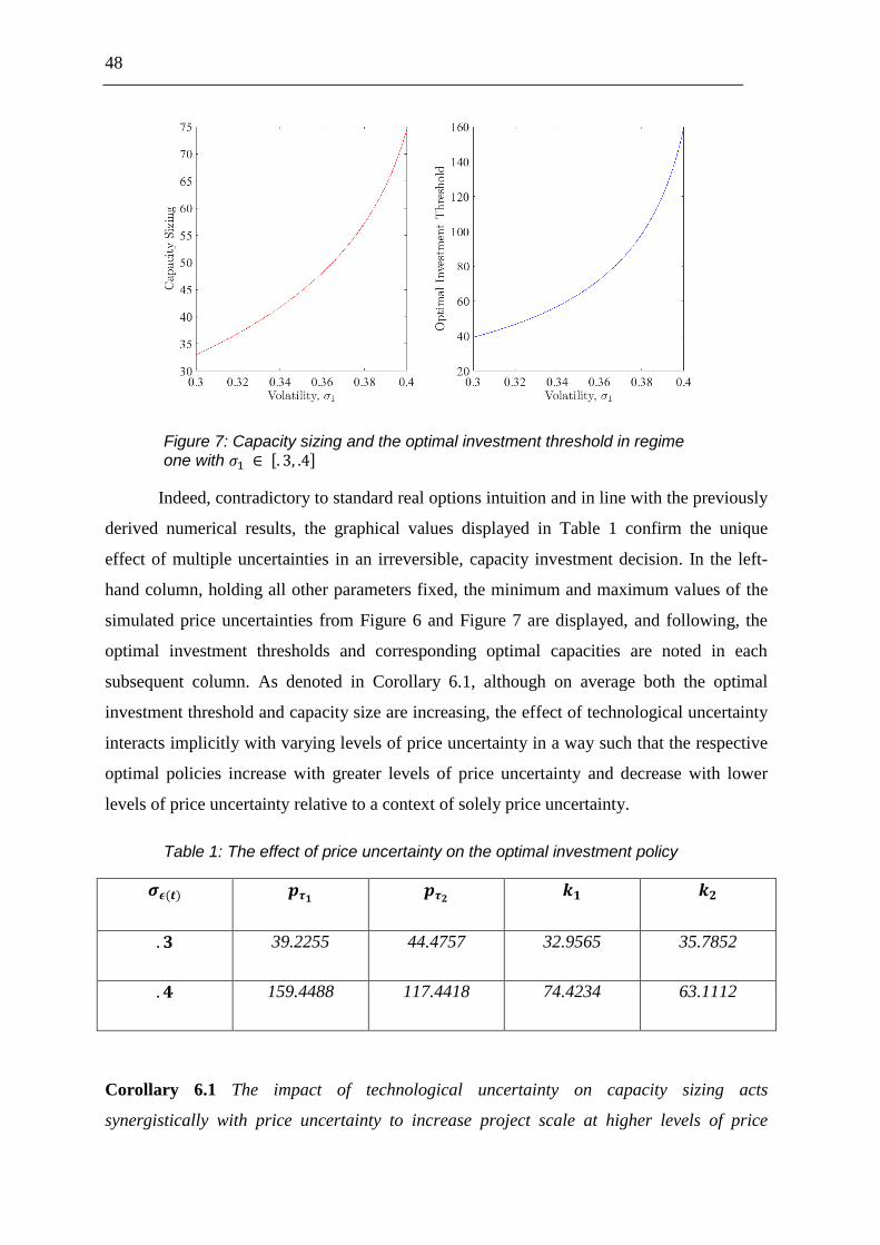
48

Figure 7: Capacity sizing and the optimal investment threshold in regime one with

Indeed, contradictory to standard real options intuition and in line with the previously

derived numerical results, the graphical values displayed in Table 1 confirm the unique

effect of multiple uncertainties in an irreversible, capacity investment decision. In the left-

hand column, holding all other parameters fixed, the minimum and maximum values of the

simulated price uncertainties from Figure 6 and Figure 7 are displayed, and following, the

optimal investment thresholds and corresponding optimal capacities are noted in each

subsequent column. As denoted in Corollary 6.1, although on average both the optimal

investment threshold and capacity size are increasing, the effect of technological uncertainty

interacts implicitly with varying levels of price uncertainty in a way such that the respective

optimal policies increase with greater levels of price uncertainty and decrease with lower

levels of price uncertainty relative to a context of solely price uncertainty.

Table 1: The effect of price uncertainty on the optimal investment policy

39.2255 44.4757 32.9565 35.7852

159.4488 117.4418 74.4234 63.1112

Corollary 6.1 The impact of technological uncertainty on capacity sizing acts

synergistically with price uncertainty to increase project scale at higher levels of price

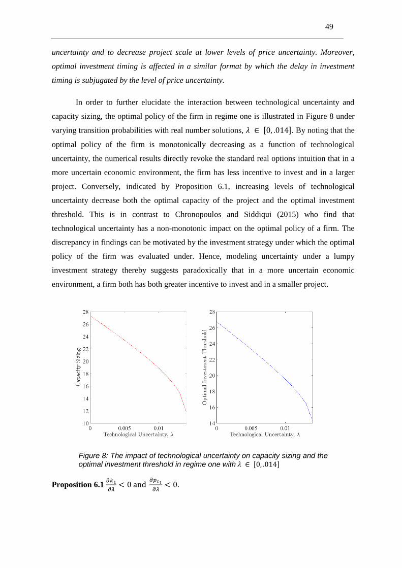
49

uncertainty and to decrease project scale at lower levels of price uncertainty. Moreover,

optimal investment timing is affected in a similar format by which the delay in investment

timing is subjugated by the level of price uncertainty.

In order to further elucidate the interaction between technological uncertainty and

capacity sizing, the optimal policy of the firm in regime one is illustrated in Figure 8 under

varying transition probabilities with real number solutions, . By noting that the

optimal policy of the firm is monotonically decreasing as a function of technological

uncertainty, the numerical results directly revoke the standard real options intuition that in a

more uncertain economic environment, the firm has less incentive to invest and in a larger

project. Conversely, indicated by Proposition 6.1, increasing levels of technological

uncertainty decrease both the optimal capacity of the project and the optimal investment

threshold. This is in contrast to Chronopoulos and Siddiqui (2015) who find that

technological uncertainty has a non-monotonic impact on the optimal policy of a firm. The

discrepancy in findings can be motivated by the investment strategy under which the optimal

policy of the firm was evaluated under. Hence, modeling uncertainty under a lumpy

investment strategy thereby suggests paradoxically that in a more uncertain economic

environment, a firm both has both greater incentive to invest and in a smaller project.

Figure 8: The impact of technological uncertainty on capacity sizing and the optimal investment threshold in regime one with

Proposition 6.1

50

7. Conclusion

This thesis set out to examine a firm’s choice in project scale under both price and

technological uncertainty, and, in order to address the potential disastrous effects of

disruptive technology on a firm operating within an incumbent technology industry,

established an analytical framework combining both regime-switching and real options. In

the context of a continuous time model where investments have a lumpy structure,

managerial insight was provided through the observation of the interactions between price

and technological uncertainty as well as the optimal investment threshold and corresponding

optimal capacity choice for a firm. Under these circumstances, the question of how an

investment decision in capacity sizing is affected by price and technological uncertainty was

scrutinized with the formulation of four propositions, one remark, a corollary, and numerical

results to provide a comprehensive answer.

In further regards to the analytical results, conclusive derivations highlighting insight

on the immediate investment decision were provided by both separately and simultaneously

comparing technological and price uncertainty. Although results were confined by a

nonlinear equation in regime one, the immediate investment decision in both scenarios was

aided by deriving a guiding function where optimal capacity choice could be determined by

the current output price of an incumbent technology. Furthermore, although expected,

managerial insight was quantitatively reinforced by the conclusion that capital investment in

an incumbent technology should decrease with increasing levels of technological

uncertainty. Lastly, leveraging Christensen’s theory of disruptive technology, further

managerial insight was provided to the firm by advising discovery-driven planning when

holding the option to invest under technological uncertainty.

In regards to the numerical results, the synergy between the two uncertainties was

examined as well as their effect on the optimal investment threshold and the corresponding

optimal capacity. Interestingly, although in standard capacity sizing literature it is generally

concluded that uncertainty leads to delayed investment and larger optimal capacity sizing,

this relationship was revoked when capacity sizing was examined under price and

technological uncertainty. Indeed, under solely price uncertainty and managerial discretion

over capacity sizing and timing, the conventional result was confirmed and graphically

proven. However, by taking into consideration technological uncertainty and lower levels of

51

price uncertainty, the optimal investment strategy, numerically derived, showed that a firm

will generally invest earlier and limit capacity investment, whereas at higher levels of price

uncertainty, a firm will invest even later and in larger capacity. Furthermore, revoking

standard real options intuition and in contrast with Chronopoulos and Siddiqui (2015), it was

shown that increasing levels of technological uncertainty directly correlate with a greater

incentive to invest and in limited project scale. Hence, by revoking standard real options

intuition and highlighted by the discrepancy in findings with Chronopoulos and Siddiqui

(2015), this study emphasizes that the relationship between technological uncertainty and

project scale requires further investigation.

As such, it is interesting to note the limitations of the model. Undeniably, although it

is helpful to base managerial insight on an analytical framework with quantitative results, the

complexity of the model poses severe restrictions on its overall applicability and utility. As

the model can only support transition probabilities of as well as a real solution

set under specific parameter settings, it becomes exceedingly difficult to adapt the model for

case-specific applications where a tailored-made solution can be provided for the firm. As

this further limits the model’s micro-level utility, managerial insight can only be broadly

provided to the firm through implicit recommendations based on the aforementioned

numerical results. To circumvent these shortcomings would require the respective

uncertainties to be studied in a more deterministic sense or the firm would have to be willing

to accept a solution with a complex numerical format. However, the consequences of such

actions would severely constrict the managerial implications and insight that the model could

realistically provide. Accordingly, as no simple solution exists, either a simpler model would

need to be constructed to provide a full analytical solution or the trade-off between model

complexity and design would have to be revisited with the firm to realistically decide an

acceptable level of quantitative insight.

Nonetheless, in order to extend these results and to further examine the effect of

technological uncertainty on project scale, there are many different avenues one could

pursue based on this study. In the area of managerial flexibilities, one could additional see

how allowing a firm the flexiblity to choose among differing investment strategies such as in

Chronopoulos and Siddiqui (2015) could change the resulting optimal policy. Additionally,

in order to examine the robustness of these results and further scrutinize flexbility,

loosening of the clearnace assumption via discretion over the production decision as in Kort

52

et al. (2011) could provide invalauble intuition to the firm’s investment decision. Operational

flexibility could also be examined as in Hagspiel et al. (2013) through the introduction of an

abandonment option or, similarly, with the simultaneous relaxation of the clearance

assumption, a suspension and resumption option could be introduced. Moreover, in a flexible

context, game-theoretic considerations could also be considered as in Goto et al. (2012) to

see how competitive analysis affects the firm’s optimal policy. In terms of model

parameters, although it would be expected to produce similar results in the majority of cases,

modeling the output price akin to the inverse demand function used by Dangl (1999) would

provide further interesting insight to capital intensive projects. Likewise, varying the type of

stochastic process implemented in the model such as mean reversion or arithmetic Brownian

motion could provide a means in which to further results as well as to provide the proper

standpoint specific to the subjective, managerial view of output price. Lastly, in the area of

uncertainty, as the model has a particular fit for the renewable energy industry given its

convex investment cost function, environmental policy uncertainty would also be interesting

to study, which could furthermore be extended by switching to a concave cost function to

cover government policy uncertainty based on welfare analysis.

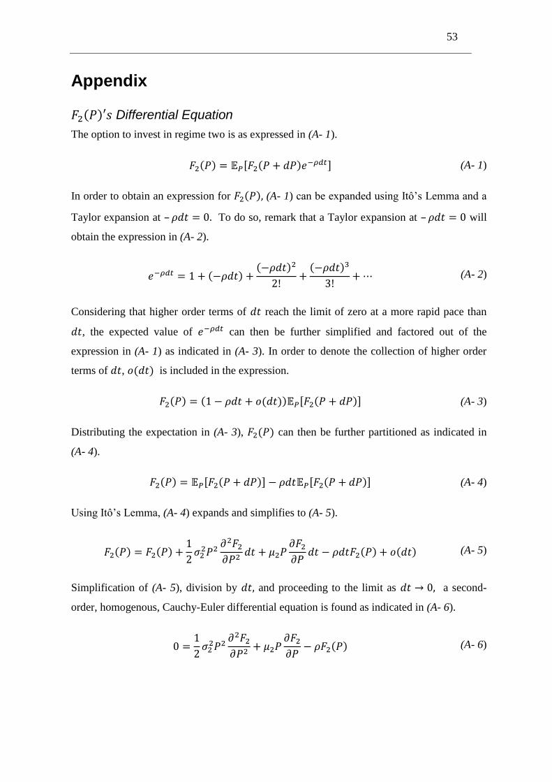
53

Appendix

Differential Equation

The option to invest in regime two is as expressed in (A- 1).

(A- 1)

In order to obtain an expression for (A- 1) can be expanded using Itô’s Lemma and a

Taylor expansion at – To do so, remark that a Taylor expansion at – will

obtain the expression in (A- 2).

(A- 2)

Considering that higher order terms of reach the limit of zero at a more rapid pace than

, the expected value of can then be further simplified and factored out of the

expression in (A- 1) as indicated in (A- 3). In order to denote the collection of higher order

terms of , is included in the expression.

(A- 3)

Distributing the expectation in (A- 3), can then be further partitioned as indicated in

(A- 4).

(A- 4)

Using Itô’s Lemma, (A- 4) expands and simplifies to (A- 5).

(A- 5)

Simplification of (A- 5), division by and proceeding to the limit as a second-

order, homogenous, Cauchy-Euler differential equation is found as indicated in (A- 6).

(A- 6)

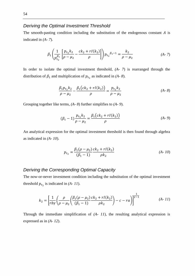
54

Deriving the Optimal Investment Threshold

The smooth-pasting condition including the substitution of the endogenous constant is

indicated in (A- 7).

(A- 7)

In order to isolate the optimal investment threshold, (A- 7) is rearranged through the

distribution of and multiplication of as indicated in (A- 8).

(A- 8)

Grouping together like terms, (A- 8) further simplifies to (A- 9).

(A- 9)

An analytical expression for the optimal investment threshold is then found through algebra

as indicated in (A- 10).

(A- 10)

Deriving the Corresponding Optimal Capacity

The now-or-never investment condition including the substitution of the optimal investment

threshold is indicated in (A- 11).

(A- 11)

Through the immediate simplification of (A- 11), the resulting analytical expression is

expressed as in (A- 12).

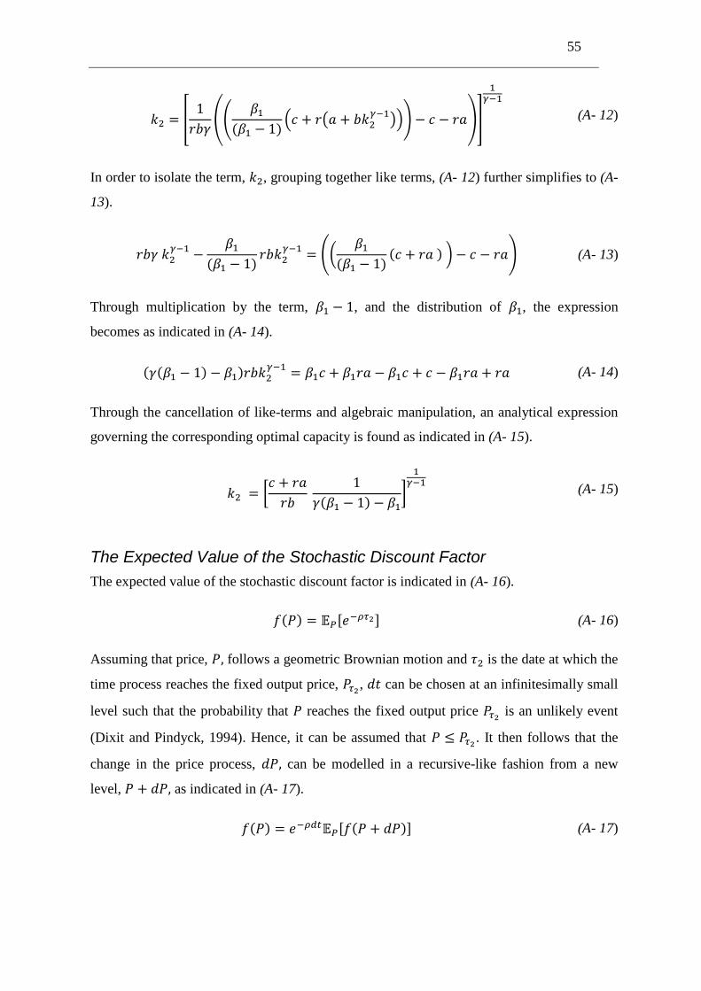
55

(A- 12)

In order to isolate the term, , grouping together like terms, (A- 12) further simplifies to (A-

13).

(A- 13)

Through multiplication by the term, , and the distribution of , the expression

becomes as indicated in (A- 14).

(A- 14)

Through the cancellation of like-terms and algebraic manipulation, an analytical expression

governing the corresponding optimal capacity is found as indicated in (A- 15).

(A- 15)

The Expected Value of the Stochastic Discount Factor

The expected value of the stochastic discount factor is indicated in (A- 16).

(A- 16)

Assuming that price, follows a geometric Brownian motion and is the date at which the

time process reaches the fixed output price, , can be chosen at an infinitesimally small

level such that the probability that reaches the fixed output price is an unlikely event

(Dixit and Pindyck, 1994). Hence, it can be assumed that . It then follows that the

change in the price process, can be modelled in a recursive-like fashion from a new

level, as indicated in (A- 17).

(A- 17)

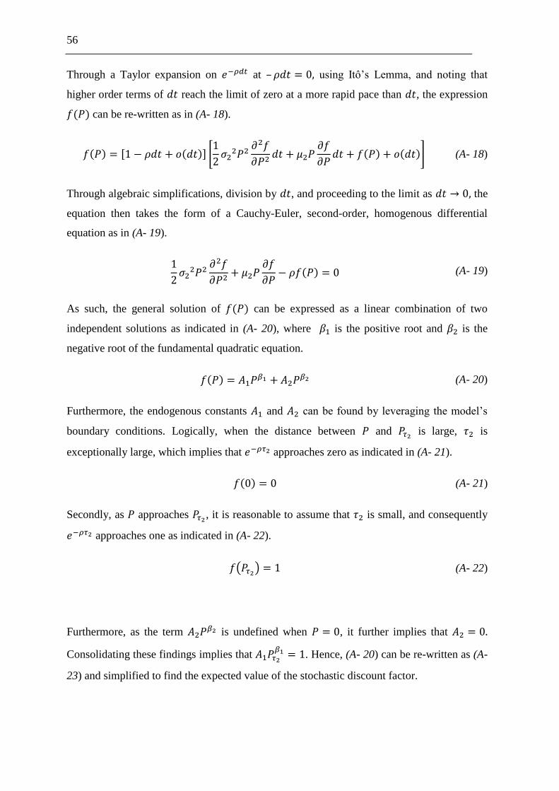
56

Through a Taylor expansion on at – using Itô’s Lemma, and noting that

higher order terms of reach the limit of zero at a more rapid pace than , the expression

can be re-written as in (A- 18).

(A- 18)

Through algebraic simplifications, division by , and proceeding to the limit as the

equation then takes the form of a Cauchy-Euler, second-order, homogenous differential

equation as in (A- 19).

(A- 19)

As such, the general solution of can be expressed as a linear combination of two

independent solutions as indicated in (A- 20), where is the positive root and is the

negative root of the fundamental quadratic equation.

(A- 20)

Furthermore, the endogenous constants and can be found by leveraging the model’s

boundary conditions. Logically, when the distance between and is large, is

exceptionally large, which implies that approaches zero as indicated in (A- 21).

(A- 21)

Secondly, as approaches , it is reasonable to assume that is small, and consequently

approaches one as indicated in (A- 22).

(A- 22)

Furthermore, as the term is undefined when , it further implies that

Consolidating these findings implies that . Hence, (A- 20) can be re-written as (A-

23) and simplified to find the expected value of the stochastic discount factor.

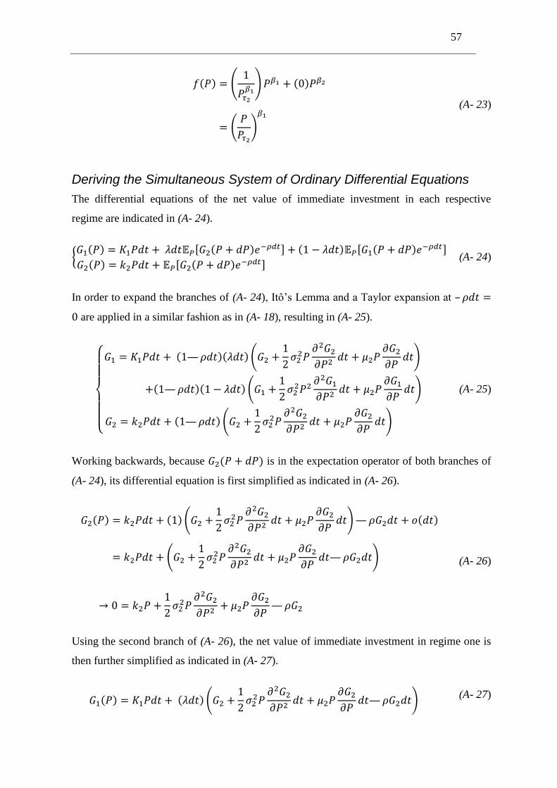
57

(A- 23)

Deriving the Simultaneous System of Ordinary Differential Equations

The differential equations of the net value of immediate investment in each respective

regime are indicated in (A- 24).

(A- 24)

In order to expand the branches of (A- 24), Itô’s Lemma and a Taylor expansion at –

are applied in a similar fashion as in (A- 18), resulting in (A- 25).

(A- 25)

Working backwards, because is in the expectation operator of both branches of

(A- 24), its differential equation is first simplified as indicated in (A- 26).

(A- 26)

Using the second branch of (A- 26), the net value of immediate investment in regime one is

then further simplified as indicated in (A- 27).

(A- 27)

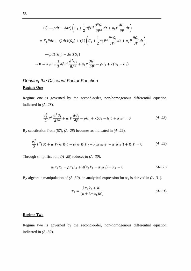
58

Deriving the Discount Factor Function

Regime One

Regime one is governed by the second-order, non-homogenous differential equation

indicated in (A- 28).

(A- 28)

By substitution from (57), (A- 28) becomes as indicated in (A- 29).

(A- 29)

Through simplification, (A- 29) reduces to (A- 30).

(A- 30)

By algebraic manipulation of (A- 30), an analytical expression for is derived in (A- 31).

(A- 31)

Regime Two

Regime two is governed by the second-order, non-homogenous differential equation

indicated in (A- 32).

59

(A- 32)

By substitution, from Equation (57), (A- 32) becomes as indicated in (A- 33).

(A- 33)

Through simplification, (A- 33) reduces to (A- 34).

(A- 34)

By algebraic manipulation of (A- 34), an analytical expression for is derived in (A- 35).

(A- 35)

By inserting (A- 35) into (A- 31) and through further algebraic manipulations, the discount

factor function is derived in (A- 36).

(A- 36)

Differential Equation

The option to invest in regime one is as expressed in (A- 37).

(A- 37)

In order to expand (A- 37), Itô’s Lemma and a Taylor expansion at – are applied in

a similar fashion as in (A- 18), resulting in (A- 38).

(A- 38)

Further simplifications of (A- 38) yield (A- 39).

60

(A- 39)

By combining like-terms, division by and proceeding to the limit as a second-

order, non-homogenous, Cauchy-Euler differential equation is found as indicated in (A- 40).

(A- 40)

Deriving the Endogenous Constant

The form of the particular solution is indicated in (A- 41).

(A- 41)

Noting that insertion of (A- 41) into (A- 40) yields the expression (A- 42).

(A- 42)

By simplification and grouping together like-terms, (A- 42) becomes (A- 43).

(A- 43)

Through algebraic manipulations of (A- 43), an analytical expression for the endogenous

constant is then derived in (A- 44).

(A- 44)

61

List of References

ANG, A. & TIMMERMANN, A. 2012. Regime Changes and Financial Markets. Annual

Review of Financial Economics, 4, 313-337.

BALCER, Y. & LIPPMAN, S. A. 1984. Technological Expectations and Adoption of

Improved Technology. Journal of Economic Theory, 34, 292-318.

BAR-ILAN, A. & STRANGE, W. C. 1999. The Timing and Intensity of Investment.

Journal of Macroeconomics, 21, 57-77.

BELLMAN, R. 1954. The Theory of Dynamic Programming. Annual Summer Meeting of

the American Mathematical Society. Laramie, Wyoming: Rand Corporation Santa

Monica.

BLOOM, N. 2009. The Impact of Uncertainty Shocks. Econometrica, 77, 623-685.

BOTTERUD, A. & KORPÅS, M. 2007. A Stochastic Dynamic Model for Optimal Timing

of Investments in New Generation Capacity in Restructured Power Systems.

International Journal of Electrical Power and Energy Systems, 29, 163-174.

BØCKMAN, T., FLETEN, S.-E., JULIUSSEN, E., LANGHAMMER, H. J. & REVDAL, I.

2008. Investment Timing and Optimal Capacity Choice for Small Hydropower

Projects. European Journal of Operational Research, 190, 255-267.

CAPOZZA, D. R. & SICK, G. A. 1994. The Risk Structure of Land Markets. Journal of

Urban Economics, 35, 297-319.

CHIB, S. 1998. Estimation and Comparison of Multiple Change-Point Models. Journal of

Econometrics, 86, 221-241.

CHOD, J. & RUDI, N. 2005. Resource Flexibility with Responsive Pricing. Operations

Research, 53, 532-548.

CHRISTENSEN, C. M. 2000. The Innovator's Dilemma, New York, HarperBusiness.

CHRONOPOULOS, M., HAGSPIEL, V. & FLETEN, S.-E. 2015. Stepwise Investment and

Capacity Sizing Under Uncertainty. Bergen: Norwegian School of Economics,

Department of Business and Management Science.

CHRONOPOULOS, M. & SIDDIQUI, A. 2015. When Is It Better to Wait for a New

Version?: Optimal Replacement of an Emerging Technology Under Uncertainty.

Annals of Operations Research, 1-25.

CHUNG, K. H. & CHAROENWONG, C. 1991. Investment Options, Assets in Place, and

the Risk of Stocks. Financial Management, 20, 21-33.

CORTAZAR, G. & SCHWARTZ, E. S. 1998. Monte Carlo Evaluation Model of an

Undeveloped Oil Field. Journal of Energy Finance and Development, 3, 73-84.

DANGL, T. 1999. Investment and Capacity Choice Under Uncertain Demand. European

Journal of Operational Research, 117, 415-428.

DELLA SETA, M., GRYGLEWICZ, S. & KORT, P. M. 2012. Optimal Investment in

Learning-Curve Technologies. Journal of Economic Dynamics and Control, 36,

1462-1476.

DIAS, M. A. G. 2004. Valuation of Exploration and Production Assets: An Overview of

Real Options Models. Journal of Petroleum Science and Engineering, 44, 93-114.

DIXIT, A. K. & PINDYCK, R. S. 1994. Investment Under Uncertainty, Princeton, N.J,

Princeton University Press.

DORASZELSKI, U. 2001. The Net Present Value Method Versus the Option Value of

Waiting: A Note on Farzin, Huisman and Kort (1998). Journal of Economic

Dynamics and Control, 25, 1109-1115.

DOUGLAS-WESTWOOD 2010. Offshore Wind Assessment for Norway.

http://www.nve.no: The Research Council of Norway.

62

EKERN, S. 1988. An Option Pricing Approach to Evaluating Petroleum Projects. Energy

Economics, 10, 91-99.

FARZIN, Y. H., HUISMAN, K. J. M. & KORT, P. M. 1998. Optimal Timing of Technology

Adoption. Journal of Economic Dynamics and Control, 22, 779-799.

FISHER, I. 1930. The Theory of Interest: As Determined by Impatience to Spend Income and

Opportunity to Invest It, New York, Macmillan.

GOTO, M., NISHIDE, K. & TAKASHIMA, R. 2012. Irreversible Investment Under

Competition with a Markov Switching Regime. SSRN Working Paper Series.

HAGSPIEL, V., JESUS, P., KORT, P. & NUNES, C. 2013. Technological Change: A

Burden or a Chance. Annual International Real Options Conference.

HUANG, J. & MCELROY, M. B. 2015. A 32- Year Perspective on the Origin of Wind

Energy in a Warming Climate. Renewable Energy, 77, 482-492.

HUBBARD, R. 1994. Investment Under Uncertainty: Keeping One's Options Open. Journal

of Economic Literature, 32, 1828.

HUBERTS, N. D., HUISMAN, K. M., KORT, P. & LAVRUTICH, M. 2015. Capacity

Choice in (Strategic) Real Options Models: A Survey. Dynamic Games and

Applications, 1-16.

HUISMAN, K. J. M. & KORT, P. M. 2004. Strategic Technology Adoption Taking into

Account Future Technological Improvements: A Real Options Approach. European

Journal of Operational Research, 159, 705-728.

INSLEY, M. C. & WIRJANTO, T. S. 2010. Contrasting Two Approaches in Real Options

Valuation: Contingent Claims Versus Dynamic Programming. Journal of Forest

Economics, 16, 157-176.

INTERNATIONAL RENEWABLE ENERGY AGENCY 2012. Wind Power. Renewable

Energy Technologies: Cost Analysis Series. www.irena.org/Publications.

KELLOGG, D. & CHARNES, J. M. 2000. Real-Options Valuation for a Biotechnology

Company. Financial Analysts Journal, 56, 76-84.

KEMNA, A. G. Z. 1993. Case Studies on Real Options. Financial Management, 22, 259-

270.

KESTER, W. 1984. Today's Options for Tomorrow's Growth. Harvard Business Review, 62,

153.

KORT, P., HUISMAN, K. & HAGSPIEL, V. 2011. Production Flexibility and Capacity

Investment Under Demand Uncertainty. Available:

http://www.researchgate.net/publication/266574056.

KULATILAKA, N. & MARKS, S. G. 1988. The Strategic Value of Flexibility: Reducing

the Ability to Compromise. The American Economic Review, 78, 574-580.

LUCAS, H. C. & GOH, J. M. 2009. Disruptive Technology: How Kodak Missed the Digital

Photography Revolution. Journal of Strategic Information Systems, 18, 46-55.

MADAR, D. 2009. Big Steel: Technology, Trade, and Survival in a Global Market, UBC

Press.

MAJD, S. & PINDYCK, R. S. 1987. Time to Build, Option Value, and Investment

Decisions. Journal of Financial Economics, 18, 7-27.

MANNE, A. S. 1961. Capacity Expansion and Probabilistic Growth. Econometrica, 29, 632-

649.

MANYIKA, J., CHUI, M., BUGHIN, J., DOBBS, R., BISSON, P. & MARRS, A. 2013.

Disruptive Technologies: Advances That Will Transform Life, Business, and the

Global Economy. McKinsey Global Institute.

MCDONALD, R. & SIEGEL, D. 1986. The Value of Waiting to Invest. The Quarterly

Journal of Economics, 101, 707-728.

63

MORRIS, P., TEISBERG, E. & KOLBE, A. 1991. When Choosing R&D Projects, Go with

Long Shots. Research Technology Management, 34, 35.

MUI, C. 2012. How Kodak Failed. Available:

http://www.forbes.com/sites/chunkamui/2012/01/18/how-kodak-failed/ [Accessed 15

August 2015].

MYERS, S. C. 1977. Determinants of Corporate Borrowing. Journal of Financial

Economics, 5, 147-175.

PETTENUZZO, D., TIMMERMANN, A. & VALKANOV, R. 2014. Forecasting Stock

Returns Under Economic Constraints. Journal of Financial Economics, 114, 517-

553.

PÁSTOR, Ľ. & STAMBAUGH, R. F. 2001. The Equity Premium and Structural Breaks.

Journal of Finance, 56, 1207-1239.

QUIGG, L. 1993. Empirical Testing of Real Option‐Pricing Models. Journal of Finance, 48,

621-640.

THE ECONOMIST. 2012. The Last Kodak Moment? Available:

http://www.economist.com/node/21542796 [Accessed 14 September 2015].

THE ECONOMIST. 2015. What Disruptive Innovation Means. Available:

http://www.economist.com/blogs/economist-explains/2015/01/economist-explains-

15 [Accessed 12 August 2015].

TITMAN, S. 1985. Urban Land Prices Under Uncertainty. The American Economic Review,

75, 505-514.

TOURINHO, O. A. F. 1979. The Valuation of Reserves of Natural Resources: An Option

Pricing Approach. Doctor of Philosophy in Business Administration, University of

California, Berkeley.

UNITED NATIONS ENVIRONMENT PROGRAMME 2015. Global Trends in Renewable

Energy Investment 2015. In: MCCRONE, A., MOSLENER, U., USHER, E.,

GRUNING, C. & SONNTAG-O'BRIEN, V. (eds.) Global Trends Report. FS-UNEP

Collaborating Centre.

VENETSANOS, K., ANGELOPOULOU, P. & TSOUTSOS, T. 2002. Renewable Energy

Sources Project Appraisal Under Uncertainty: The Case of Wind Energy Exploitation

Within a Changing Energy Market Environment. Energy Policy, 30, 293-307.