Embed Size (px)
Citation preview

NoSQL Data Store Technologies
John Klein, Software Engineering Institute Patrick Donohoe, Software Engineering Institute Neil Ernst, Software Engineering Institute Ian Gorton, Software Engineering Institute Chrisjan Matser, U.S Army Medical Research and Materiel Command (MRMC) Telemedicine and
Advanced Technology Research Center (TATRC) Kim Pham, U.S Army Medical Research and Materiel Command (MRMC) Telemedicine and Advanced
Technology Research Center (TATRC)
September 2014
FINAL REPORT V1.1 TATRC BIG DATA INVESTIGATION FINAL REPORT
http://www.sei.cmu.edu

Report Documentation Page Form ApprovedOMB No. 0704-0188
Public reporting burden for the collection of information is estimated to average 1 hour per response, including the time for reviewing instructions, searching existing data sources, gathering andmaintaining the data needed, and completing and reviewing the collection of information. Send comments regarding this burden estimate or any other aspect of this collection of information,including suggestions for reducing this burden, to Washington Headquarters Services, Directorate for Information Operations and Reports, 1215 Jefferson Davis Highway, Suite 1204, ArlingtonVA 22202-4302. Respondents should be aware that notwithstanding any other provision of law, no person shall be subject to a penalty for failing to comply with a collection of information if itdoes not display a currently valid OMB control number.
1. REPORT DATE 01 SEP 2014
2. REPORT TYPE N/A
3. DATES COVERED
4. TITLE AND SUBTITLE NoSQL Data Store Technologies
5a. CONTRACT NUMBER
5b. GRANT NUMBER
5c. PROGRAM ELEMENT NUMBER
6. AUTHOR(S) John Klein Patrick Donohoe /Neil Ernst, Ian Gorton, Kim Pham,Chrisjan Matser
5d. PROJECT NUMBER
5e. TASK NUMBER
5f. WORK UNIT NUMBER
7. PERFORMING ORGANIZATION NAME(S) AND ADDRESS(ES) Software Engineering Institute Carnegie Mellon University Pittsburgh,PA 15213
8. PERFORMING ORGANIZATIONREPORT NUMBER
9. SPONSORING/MONITORING AGENCY NAME(S) AND ADDRESS(ES) 10. SPONSOR/MONITOR’S ACRONYM(S)
11. SPONSOR/MONITOR’S REPORT NUMBER(S)
12. DISTRIBUTION/AVAILABILITY STATEMENT Approved for public release, distribution unlimited.
13. SUPPLEMENTARY NOTES
14. ABSTRACT
15. SUBJECT TERMS
16. SECURITY CLASSIFICATION OF: 17. LIMITATION OF ABSTRACT
SAR
18. NUMBEROF PAGES
76
19a. NAME OFRESPONSIBLE PERSON
a. REPORT unclassified
b. ABSTRACT unclassified
c. THIS PAGE unclassified
Standard Form 298 (Rev. 8-98) Prescribed by ANSI Std Z39-18

Copyright 2014 Carnegie Mellon University
This material is based upon work funded and supported by the Department of Defense under Contract No. FA8721-05-C-0003 with Carnegie Mellon University for the operation of the Software Engineering Institute, a federally funded research and development center.
Any opinions, findings and conclusions or recommendations expressed in this material are those of the author(s) and do not necessarily reflect the views of the United States Department of Defense.
References herein to any specific commercial product, process, or service by trade name, trade mark, manufacturer, or otherwise, does not necessarily constitute or imply its endorsement, recommendation, or favoring by Carnegie Mellon University or its Software Engineering Institute.
NO WARRANTY. THIS CARNEGIE MELLON UNIVERSITY AND SOFTWARE ENGINEERING INSTITUTE MATERIAL IS FURNISHED ON AN “AS-IS” BASIS. CARNEGIE MELLON UNIVERSITY MAKES NO WARRANTIES OF ANY KIND, EITHER EXPRESSED OR IMPLIED, AS TO ANY MATTER INCLUDING, BUT NOT LIMITED TO, WARRANTY OF FITNESS FOR PURPOSE OR MERCHANTABILITY, EXCLUSIVITY, OR RESULTS OBTAINED FROM USE OF THE MATERIAL. CARNEGIE MELLON UNIVERSITY DOES NOT MAKE ANY WARRANTY OF ANY KIND WITH RESPECT TO FREEDOM FROM PATENT, TRADEMARK, OR COPYRIGHT INFRINGEMENT.
This material has been approved for public release and unlimited distribution except as restricted below.
Internal use:* Permission to reproduce this material and to prepare derivative works from this material for internal use is granted, provided the copyright and “No Warranty” statements are included with all reproductions and derivative works.
External use:* This material may be reproduced in its entirety, without modification, and freely distribut-ed in written or electronic form without requesting formal permission. Permission is required for any other external and/or commercial use. Requests for permission should be directed to the Software En-gineering Institute at [email protected].
* These restrictions do not apply to U.S. government entities.
T-CheckSM
DM-0001676

TATRC BIG DATA INVESTIGATION FINAL REPORT | i
Table of Contents
Abstract x
1 Introduction 1
2 Evaluation Approach/Method 2 2.1 Quality Requirements 2 2.2 Stakeholder Workshop and Development of Evaluation Criteria 2 2.3 Database Selection 4 2.4 Measurement Approach 6
3 Test Environment 7 3.1 Synthetic Data Set 7
3.1.1 Source/Contents 7 3.1.2 Schema 8
3.2 Data Models 17 3.2.1 MongoDB 17 3.2.2 Cassandra 18 3.2.3 Riak 19 3.2.4 Neo4j 20
3.3 Virtual Private Cloud 21 3.4 Bulk Load 22 3.5 Read/Write Testing and Workloads 24
3.5.1 Workload Details 25 3.5.2 Running the Workloads 26
3.6 Measurement Collection and Reporting 26 3.7 Network Partition Simulation 28
4 Results Discussion 30 4.1 Read/Write Performance Evaluation 30 4.2 Partition Tolerance 39 4.3 Bulk Load 42
4.3.1 MongoDB 42 4.3.2 Cassandra 44 4.3.3 Riak 45 4.3.4 Neo4j 46
4.4 Data Model Fit/Mapping 47 4.5 Limitations 48
4.5.1 Environment/Optimization 48 4.5.2 Scope/Coverage of Use Cases 48 4.5.3 Caching 48 4.5.4 Data Set Size 48 4.5.5 Test Client Limits 48 4.5.6 Polyglot Persistence 49
5 Conclusion 50 5.1 Lessons Learned 50
5.1.1 Technology Selection Process 50 5.1.2 Prototyping and Measurement 51
Appendix A – Scenarios Developed in Stakeholder Workshop 53

TATRC BIG DATA INVESTIGATION FINAL REPORT | ii
Appendix B – Data Analysis Workflow 55
References 62

TATRC BIG DATA INVESTIGATION FINAL REPORT | iii

TATRC BIG DATA INVESTIGATION FINAL REPORT | iv
List of Figures
Figure 1: Examples of Major NoSQL data models 5 Figure 2: A vMR-CDS Patient Model 9 Figure 3: A FHIR Patient Model 10 Figure 4: A FHIR Observation Model 10 Figure 5: Example of a FHIR Patient Resource Embedded in a MongoDB Document 11 Figure 6: Example of a FHIR Observation Resource Embedded in a MongoDB Document 12 Figure 7: Example of a FHIR Patient Resource Mapped to Cassandra 13 Figure 8: Example of a FHIR Observation Resource Mapped to Cassandra 14 Figure 9: Example of a FHIR Patient Resource Mapped to Riak 16 Figure 10: Example of a FHIR Observation Resource Mapped to Riak 17 Figure 11: MongoDB Physical Data Model 18 Figure 12: Cassandra Physical Data Model 19 Figure 13: Riak Physical Data Model 20 Figure 14: Neo4j Physical Data Model 21 Figure 15: Throughput, Single Node, Read-only Workload 31 Figure 16: Throughput, Single Node, Write-only Workload 31 Figure 17: Throughput, Single Node, Read/Write Workload 32 Figure 18: Read Latency, Single Node, Read/Write Workload 32 Figure 19: Write Latency, Single Node, Read/Write Workload 33 Figure 20: Throughput, Representative Production Configuration, Read-Only Workload 34 Figure 21: Throughput, Representative Production Configuration, Write-Only Workload 35 Figure 22: Throughput, Representative Production Configuration, Read/Write Workload 35 Figure 23: Read Latency, Representative Production Configuration, Read/Write Workload 36 Figure 24: Write Latency, Representative Production Configuration, Read/Write Workload 36 Figure 25: Read Latency, Representative Production Configuration, Read/Write Workload 37 Figure 26: Write Latency, Representative Production Configuration, Read/Write Workload 37 Figure 27: Cassandra – Comparison of strong consistency and eventual consistency 38 Figure 28: Riak – Comparison of strong consistency and eventual consistency 39 Figure 29: Network configuration for partition testing of MongoDB 39 Figure 30: MongoDB “acknowledged” write concern 40 Figure 31: Impact of partition on MongoDB insert operation latency 41 Figure 32: Impact of network latency on MongoDB insert operation throughput 41 Figure 33: Bulk load latency vs threads 44

TATRC BIG DATA INVESTIGATION FINAL REPORT | v
Figure 34: Bulk load latency vs operations 46

TATRC BIG DATA INVESTIGATION FINAL REPORT | vi

TATRC BIG DATA INVESTIGATION FINAL REPORT | vii
List of Tables
Table 1: Stakeholder Workshop Attendees 3 Table 2: Consolidated Scenarios Related to Core EHR Access Tasks 3 Table 3: Workload definitions for YCSB 25 Table 4: Write and read settings for representative production configuration 34 Table 5: Write and read settings for eventual consistency configuration 38 Table 6: Bulk Write performance for each batch of 400K records. 42 Table 7: Serial Write performance for each batch of 400K records. 43 Table 8: Read performances after inserting each batch of 400K records. 43 Table 9: Read performances after inserting each batch of 400K records. 44 Table 10: Bulk load performances for bucket “Observation” 45

TATRC BIG DATA INVESTIGATION FINAL REPORT | viii

TATRC BIG DATA INVESTIGATION FINAL REPORT | ix

TATRC BIG DATA INVESTIGATION FINAL REPORT | x
Abstract
The Interagency Program Office has been exploring a number of options for interoperation be-tween the electronic health record systems used by DoD and the Veteran’s Health Administration. These have included replacing both systems with a single new Integrated Electronic Health Rec-ord (iEHR) system and federating the information contained in existing systems, among other approaches. In addition, DoD has been exploring caching approaches to improve delivery of elec-tronic health record applications over network links with low quality of service. The Military Health System’s Joint Program Committee funded the Army Telemedicine and Advanced Tech-nology Research Center (TATRC) to work with the SEI to investigate the use of emerging NoSQL database technology to achieve the data storage capabilities needed for these systems.
The SEI conducted a stakeholder workshop with MHS stakeholders to identify architecture driv-ers and quality attribute requirements for these applications. These requirements were then used to create technology evaluation criteria.
The SEI then worked with developers from the TATRC Advanced Concepts Team to conduct a series of technology experiments to assess the suitability of several NoSQL products against the evaluation criteria. One NoSQL product was selected for evaluation from each of the four NoSQL categories: Document Store (MongoDB), Column Family Store (Cassandra), Key-Value Store (Riak), and Graph Store (Neo4J). Each product was installed in a server cluster in the SEI Virtual Private Cloud, and performance measurements were made for each using the YCSB (Yahoo! Cloud Serving Benchmark) test driver. Several workloads were tested, including read-only, write-only, bulk load, and mixed read/write. Testing was also conducted to assess performance of the server cluster when there are network delays or partitions.
The findings included both qualitative and quantitative results. Qualitative results included how well the information model of the electronic health record fit with each of the NoSQL data models and an assessment of ease of software development and integration with the product. Quantitative results were analyzed to identify key “go/no-go” sensitivity points and tradeoffs (e.g., data model, number of servers in the cluster, consistency models, and simultaneous client sessions) that can be used to narrow the solution space to a small number of candidate products, which can then be evaluated in more detail. There was minimal database and server tuning, so the results presented in this report should not be interpreted to represent achievable performance levels for any of the tested products.
This report discusses both qualitative and quantitative results, and includes all data collected dur-ing the conduct of the technology experiments.

TATRC BIG DATA INVESTIGATION FINAL REPORT | xi

TATRC BIG DATA INVESTIGATION FINAL REPORT | 1
1 Introduction
The Interagency Program Office has been exploring a number of options for interoperation be-tween the electronic health record systems used by DoD and the Veteran’s Health Administration. These have included replacing both systems with a single new Integrated Electronic Health Rec-ord (iEHR) system and federating the information contained in existing systems, among other approaches. In addition, DoD has been exploring caching approaches to improve delivery of elec-tronic health record applications over network links with low quality of service. The Military Health System’s Joint Program Committee funded the Army Telemedicine and Advanced Tech-nology Research Center (TATRC) to work with the SEI to investigate the use of emerging NoSQL database technology to achieve the data storage capabilities needed for these systems.
The SEI conducted a stakeholder workshop with MHS stakeholders to identify architecture driv-ers and quality attribute requirements for these applications. These requirements were then used to create technology evaluation criteria. The workshop and criteria development are described in Sections 2.1 and 2.2 below.
The SEI then worked with developers from the TATRC Advanced Concepts Team to conduct a series of technology experiments to assess the suitability of several NoSQL products against the evaluation criteria. This began by selecting one NoSQL product for evaluation from each of the four NoSQL categories: Document Store (MongoDB), Column Family Store (Cassandra), Key-Value Store (Riak), and Graph Store (neo4J). This is described further in Section 2.3 below.
The measurement approach is described in Section 2.4 below. Each product was installed in a server cluster in the SEI Virtual Private Cloud, and performance measurements were made for each using the YCSB (Yahoo! Cloud Serving Benchmark) test driver. Several workloads were tested, including read-only, write-only, bulk load, and mixed read/write. Testing was also con-ducted to assess performance of the server cluster when there are network delays or partitions. Section 3 provides details of the environment used to execute the tests and analyze the results.
The findings include both qualitative and quantitative results, detailed in Section 4. Qualitative results include how well the information model of the electronic health record fit with each of the NoSQL data models and an assessment of ease of software development and integration with the product. Quantitative results identify key “go/no-go” sensitivity points and tradeoffs (e.g., data model, number of servers in the cluster, consistency models, and simultaneous client sessions) that can be used to narrow the solution space to a small number of candidate products, which can then be evaluated in more detail. There was minimal database and server tuning, so the results presented in this report should not be interpreted to represent achievable performance levels for any of the tested products.
This report discusses both overall qualitative and quantitative results. All data collected during the conduct of the technology experiments is provided separately via electronic distribution.

TATRC BIG DATA INVESTIGATION FINAL REPORT | 2
2 Evaluation Approach/Method
2.1 Quality Requirements
This project evaluated big data technologies using a set of quality attribute requirements that are cross-cutting and pervasive in scalable database applications. We used a systematic approach that can be generalized for any project to selecting a NoSQL database that can satisfy its requirements. This approach reduces the risks of needing to migrate to a new database management system downstream by ensuring a thorough evaluation of the solution space is carried out in the minimum of time and with minimum effort.
A key feature of our approach is its NoSQL database feature evaluation criteria. This ready-made set of criteria significantly speeds up a NoSQL database evaluation and acquisition effort. To this end, we have categorized the major characteristics of data management technologies based upon the following areas:
1. Data Model – categorizes core data organization principles provided by a NoSQL database
2. Query Language – characterizes the API and specific data manipulation features supported by a NoSQL database
3. Data Distribution – analyzes the software architecture and mechanisms that are used by a NoSQL database to distribute data
4. Data Replication – determines how a NoSQL database facilitates reliable, high performance data replication to build highly available applications
5. Consistency – categorizes the consistency model(s) that a NoSQL database offers
6. Scalability – captures the core architecture and mechanisms that support scaling a big data application in terms of both data and request load increases
7. Performance – assesses mechanisms used to provide high-performance data access 8. Security – analyzes the features of a technology for providing secure data access
9. Administration and Management – categorizes and describe the tools provided by a NoSQL database to support system administration, monitoring and management
In this report, we will further elaborate on several of these feature categories and evaluate three candidate NoSQL databases that we have worked with to prototype an EHR system use case.
2.2 Stakeholder Workshop and Development of Evaluation Criteria
On 11 Sept 2012, the SEI conducted an architecture stakeholder workshop at the SEI office in Arlington, VA. Attendees were MHS stakeholders from the Interagency Program Office, TATRC, and other organizations gathered to identify driving quality attribute requirements for the iEHR Data Repository architecture. Table 1 lists the workshop attendees and organizations represented.

TATRC BIG DATA INVESTIGATION FINAL REPORT | 3
Table 1: Stakeholder Workshop Attendees
Name Organization
David Calvin IPO/TD Dave Parker Define-IT Nathan Gould IPO/CTO Phillip Keller DHIMS Shaq Datsur Deloitte Mary Ann Wronko Mitre Ollie Gray TATRC Bob Wolfe DHIMS Kim Zirnfus DHIMS CDR Shirley Thompson DHIMS Jason Addis DHIMS Patrick Donohoe SEI Patrick Place SEI John Klein SEI Kim Pham TATRC (by telephone) Chrisjan Matser TATRC (by telephone)
There were 24 quality attribute scenarios [Barbacci 2003] created and discussed during the work-shop. These are detailed in Appendix A below. After the workshop, the scenarios were reviewed and we found that 14 of the scenarios cover core EHR access tasks – locate patient record, access and retrieve patient record, and update patient record. These core scenarios are listed in Table 2.
Table 2: Consolidated Scenarios Related to Core EHR Access Tasks
Scenario IDs (See Appendix A for details)
Comments
1 (5, 8) Implies caching to mitigate poor quality of service on wide-area net-work, related to Scenario 5 (write back) and 8 (pre-fetch).
2 (4, 6) May or may not involve caching. Similar to Scenario 4. Related to Sce-nario 6 (first responder).
3 (16, 17, 23) Updates are immediately visible – this implies event publication. Relat-ed to Scenarios 16, 17, and 23.
10 (7, 11) Disconnected operation. Related to Scenario 7 (field medic uploads “encounter” – extreme case of write back of cached data). Also related to Scenario 11 (humanitarian mission with no write back).
19 Federation of data sources (radiology images).
Based on these 14 scenarios, we identified the following concerns about the architecture and un-derlying database technology:
• How does horizontal sharding approach affect performance?
• How does replication approach affect performance?
• How is the federated healthcare data schema mapped into the physical data store?
• How does the schema mapping impact performance?
• How does data store or WAN availability affect this task?
• How does the data store process record updates?
• How does the data store support merging encounter records?
• Do updates or merges require re-indexing of the data store?

TATRC BIG DATA INVESTIGATION FINAL REPORT | 4
• How is an application informed that a record of interest has been added? Does schema map-ping or federation approach affect this task?
• How does the data store use transactions or other approaches to ensure consistency?
• How is consistency achieved if the data store or WAN is not available?
• Big bulk load of initial data set.
• Backup and restore operations
• Audit trail
• Data typing
• Programming language bindings available
These evaluation concerns were then used to select database technologies and create a prototyping and measurement plan.
2.3 Database Selection
The rise of big data applications has caused significant flux in database technologies. While ma-ture relational database technologies continue to evolve, a spectrum of databases labeled “NoSQL” has emerged in the past decade. The relational model imposes a strict schema, which inhibits data evolution and causes difficulties scaling across clusters. In response, NoSQL data-bases have adopted simpler data models. Common features include schemaless records, allowing data models to evolve dynamically, and horizontal scaling, by sharding and replicating data col-lections across large clusters. Figure 1 illustrates the four most prominent types of NoSQL data-bases, and we summarize their characteristics below. More comprehensive information can be found at http://nosql-database.org/.
• Document databases store collections of objects, typically encoded using Javascript Object Notation (JSON) or Extensible Markup Langauge (XML). Documents have keys, and sec-ondary indexes can be built on non-key fields. Document formats are self-describing, and a collection may include documents with different formats. Leading examples are MongoDB (http://www.mongodb.org/) and CouchDB (http://couchdb.apache.org/).
• Key-value databases implement a distributed hash map. Records can only be accessed through key searches, and the value associated with each key is treated as opaque, requiring reader interpretation. This simple model facilitates sharding and replication to create highly scalable and available systems. Examples are Riak (http://riak.basho.com/) and DynamoDB (http://aws.amazon.com/dynamodb/).
• Column-oriented databases extend the key-value model by organizing keyed records as a collection of columns, where a column is a key-value pair. The key becomes the column name, and the value can be an arbitrary data type such as a JSON document or a binary im-age. A collection may contain records that have different numbers of columns. Examples are HBase (http://hbase.apache.org/) and Cassandra (https://cassandra.apache.org/).
• Graph databases organize data in a highly connected structure, typically some form of di-rected graph. They can provide exceptional performance for problems involving graph tra-versals and sub-graph matching. As efficient graph partitioning is an NP-hard problem, these databases tend to be less concerned with horizontal scaling, and commonly offer ACID

TATRC BIG DATA INVESTIGATION FINAL REPORT | 5
transactions to provide strong consistency. Examples include Neo4j (http://www.neo4j.org/) and GraphBase (http://graphbase.net).
Figure 1: Examples of Major NoSQL data models
NoSQL technologies have many implications for application design. As there is no equivalent of SQL, each technology supports its own specific query mechanism. These typically make the ap-plication programmer responsible for explicitly formulating query executions, rather than relying on query planners that execute queries based on declarative specifications. The ability to combine results from different data collections also becomes the programmer’s responsibility. This lack of the ability to perform JOINs forces extensive denormalization of data models so that JOIN-style queries can be efficiently executed by accessing a single data collection. When databases are sharded and replicated, it further becomes the programmer’s responsibility to manage consistency when concurrent updates occur, and design applications to tolerate stale data due to latency in update replication.
In this project, we have performed detailed evaluations of four databases, namely:
1. MongoDB: document-oriented database
2. Cassandra: column-oriented database
3. Riak: key-value database
4. Neo4J: graph database
The measurements of Neo4J were not completed in time to be included in this report. They are included in the accompanying electronic media containing the data. These results are not relevant to the iEHR analysis, because Neo4J does not provide the powerful sharding capabilities that will be needed in the EHR system context.
“id”: “1” “Name”: “John” “Employer”: “SEI”“id”: “2” “Name”: “Ian” “Employer”: “SEI” “Previous”: “PNNL”
“key”: “1” value { “Name”: “John” “Employer”: “SEI”}“key”: “2” value {“Name”: “Ian” “Employer”: “SEI” “Previous”: “PNNL”}
“row”: “1” , “Employer” “Name”“SEI” “John”
“row”: “2” “Employer” “Name” “Previous”“SEI” “Ian” “PNNL”
Node: Employee“id”: “1” “Name”: “John”“id”: “2” “Name”:”Ian”
Node: Employer“Name”: “SEI”
“Name”:”PNNL”“previously employed by”
“is employed by”
Document Store
Key-‐Value Store
Column Store
Graph Store

TATRC BIG DATA INVESTIGATION FINAL REPORT | 6
2.4 Measurement Approach
Our systematic approach enables us to evaluate many of the key features of NoSQL technologies through a detailed analysis of their documentation. However, a thorough evaluation and compari-son requires prototyping with each technology to reveal the performance and scalability that each technology is capable of providing [Gorton 2003].
To this end, we have carried out a systematic experiment that provides a foundation for an ‘apples to apples’ comparison of the three technologies we have evaluated. The approach we have taken is as follows:
1. Define a use case from the Military Health EHR system. This requires a detailed logical data model and collection of read and write queries that will be performed upon the data. We have leveraged the FHIR standard for modeling the data [FHIR 2014].
2. Define a consistent test environment for evaluating each database. In this project we have used the SEI Virtual Private Cloud (VPC), based on Amazon’s Elastic Compute Cloud (EC2) (http://aws.amazon.com/ec2), and created a set of virtual machine (VM) images which we use to deploy each database and the test clients:
3. Map the logical data model (for patient records) to each database’s physical data model and load the resulting database with a large collection of synthetic test data.
4. Create a load test client that implements the required use case in terms of the defined read and write operations. This client is capable of executing many simultaneous requests on the database so that we analyze how each technology responds in terms of performance and scalability as the request load increases.
5. Define and execute test scripts that exert a specified load on the database using the test cli-ent. These are basically divided into three categories, namely read-only, write-only and a mix of 80% reads and 20% writes (which the workshop stakeholders asserted to be a typical mix for a military health facility). We also execute each test scripts with an increasing load, starting with one client and increasing in defined steps up to a 1000 simultaneous client re-quests.
6. For each defined test case, we have experimented with a number of configurations for each database so we can analyze performance and scalability as each database is sharded and rep-licated. These deployment scenarios range from a single server for baseline testing up to 9 server instances that shard and replicate data.
Based on this approach, we are able to produce a consistent set of test results from experiments that can be used to assess the likely performance and scalability of each database in an EHR sys-tem. These results are discussed in Section 4.

TATRC BIG DATA INVESTIGATION FINAL REPORT | 7
3 Test Environment
3.1 Synthetic Data Set
3.1.1 Source/Contents
The TATRC data set for our tests was derived from a set of ExactData synthetic data files labeled R0.DS2. From the ExactData synthetic data set, the following subsets were used to generate the TATRC data set:
• two enrollment files with a combination of 1,000,067 unique patient records
• two laboratory results files with a total of 2,097,150 unique observation records
• two pharmacy claims files with a total of 2,097,150 unique medication records
The content of the ExactData synthetic data included data elements defined on the Healthcare Information Technology Standards Panel (HITSP) C83 and C80 standards [HITSP 2010a, HITSP 2010b].1
The data files are comma-separated values (CSV) files covering the three categories of patient enrollments, laboratory results, and pharmacy claims. The data elements in each file are repre-sentative of each category of data. For example, enrollment data cover patient demographic in-formation such as name, address, age, date of birth, etc., while lab data contains information such as type of test, date, LOINC code, etc. All of the information can be replicated as needed to pro-vide datasets of a size suitable for our testing.
The TATRC data set comprises
• patient demographics records extracted from the ExactData enrollments data files,
• observation records extracted from the ExactData laboratory results data files and replicated to produce a total of ten millions records for the experiments,
• medication dispense records extracted from the ExactData pharmacy claims data files and replicated to produce a total of ten millions records for the experiments.
The actual dataset used for our experiments had the following characteristics:
• patient data
− approximately 940 bytes per record − a total of 1,000,067 records with patient date of birth ranging from 10/01/1945 to
08/31/1992 • observation data
− approximately 490 bytes per record − a total of ten million (10,000,000) records with the observations in a date range from
10/01/2010 to 09/30/2012 1 HITSP was disbanded in 2010 after its contract with the Department of Health and Human Services concluded
in 2010.

TATRC BIG DATA INVESTIGATION FINAL REPORT | 8
• Observation data distribution characteristics:
− 20% of patients having 3 observations each − 20% of patients having 4 observations each − 20% of patients having 5 observations each − 20% of patients having 6 observations each − 20% of patients having 7 observations each
• medication dispensed data
− approximately 740 bytes per record − a total of ten million (10,000,000) records
We mostly used the patient and lab data in our experiments. These two domains provided suffi-cient content for basic create/read/update/delete operations involving patient records and also met our requirement to be able to deal with the patients’ associated clinical information.
3.1.2 Schema
One of the basic requirements of the test environment was to define the “schema” of the NoSQL data stores and then populate the stores with the actual data. Although NoSQL data stores are touted as being schema-free, they do have underlying structures into which data must be mapped (e.g., MongoDB has the concept of documents and sub-documents, all contained within a collec-tion). The schema definition began with selection of a conceptual data model to represent patient and lab information extracted from the synthetic data files.
For our first round of testing, with MongoDB as the target data store, we mapped the patient and lab data entities of the synthetic data set to a data model based on the Health Level 7 (HL7) stand-ard known as vMR-CDS [VMR 2013]. The Virtual Medical Record (vMR) for Clinical Decision Support (CDS) is based on the HL7 Reference Information Model (RIM) version 3 and is comprehen-sively documented. Figure 2 is a UML diagram showing how a patient is modeled in vMR-CDS.

TATRC BIG DATA INVESTIGATION FINAL REPORT | 9
Figure 2: A vMR-CDS Patient Model
We also mapped the patient and lab data to the newer HL7 Fast Healthcare Interoperability Re-sources (FHIR) data model [FHIR 2014] and re-ran the tests for comparison. The performance differences between the vMR-CDS “flat” model and the FHIR nested model were not significant, especially for the TATRC 80-20 read-write mix, so we elected to use the FHIR data model for all further experimentation. FHIR is gaining traction as a more practical way to achieve interopera-bility without slavishly following the HL7 RIM.2
The FHIR data model is based on modular components called “Resources”. Patient information is modeled as a Patient resource and a lab result is modeled as an Observation resource. Figure 3 describes a FHIR Patient model and Figure 4 describes a FHIR Observation model.
2 The version of FHIR that we used is a draft standard for trial use (DSTU) Release 1.1 that was released in Feb-
ruary, 2014.

TATRC BIG DATA INVESTIGATION FINAL REPORT | 10
Figure 3: A FHIR Patient Model
Figure 4: A FHIR Observation Model
The following sections describe how the FHIR resources for patients and their associated lab re-sults were mapped to the “schema” of the NoSQL data stores under test. Both patient data and lab results data are represented in JavaScript object notation (JSON).
3.1.2.1 MongoDB Mapping – “Patient” and “Observation” Resources
MongoDB organizes data into collections of JSON documents (actually, to a binary form of JSON called BSON). A document can be as simple as a name-value pair, or it can contain multiple em-bedded documents. The document-oriented approach of MongoDB allows for the aggregation and nesting of related data via arrays and subdocuments within a single document, easily accommo-dating the denormalization necessary to eliminate the joins characteristic of relational database

TATRC BIG DATA INVESTIGATION FINAL REPORT | 11
queries. This is the “schema” into which the FHIR data models for patients and their lab results were mapped.
Figure 5 shows how attributes of a FHIR Patient resource (represented here in JSON) were em-bedded in a MongoDB JSON document residing in the “fhir.patient” collection.
Figure 5: Example of a FHIR Patient Resource Embedded in a MongoDB Document
Figure 6 shows how attributes of a FHIR Observation resource were embedded in a MongoDB JSON document residing in the “fhir.labdata” collection. To model the one-to-many relationship between patients and their lab results, the patient ID is embedded in the lab data documents.
{"resourceType" : "Patient","identifier" : [{"use" : "secondary“, "label" : "SSN“, "system" :
"urn:oid:2.16.840.1.113883.4.1“, "value" : "894507044”},
{“use”:"official“,"label”:"MRN“,"system“: "urn:oid:2.16.840.1.113883.3.198“,
“value" : "404074589“,"assigner" : {"display" : "Department of
Defense”}}],"name" : [{"use" : "official“, "text" : "Wyatt, Burke E“,
"family" : ["Wyatt”],"given" : ["Burke“, "E”], "prefix" : ["Mr.”]}],"telecom" : [{"system" : "phone", "value" : "(918) 206-1802“,
"use" : "home”},{"system" : "phone“, "value" : "(918) 206-1802“,
"use" : "work”}],"gender" : {"coding" : [{"system" :
http://hl7.org/fhir/v3/AdministrativeGender,"code" : "M“, "display" : "Male”}]},"birthDate" : "1961-08-21T00:00:00-07:00","address" : [{"use" : "home“,"line" : ["6934 Pettis
Road“,“Apt. 1071”],"city" : "Tulsa“,"state" : "OK“,"zip" : "74137“,"country" : "US”}],"active" : true
}
Document
{"_id": ObjectId("535623a0a586797b9d914a4f"),"_class”:
"dod.tatrc.nosql.mongodb.collection.fhir.Patient","patientId" : "404074589","createdDate" : ISODate("2014-04-22T08:09:04.132Z"),"resource" : {"resourceType" : "Patient","identifier" : [{"use" : "secondary“, "label" : "SSN“, "system" :
"urn:oid:2.16.840.1.113883.4.1“, "value" : "894507044”},{{“use" : "official“, "label" : "MRN“, "system" :
"urn:oid:2.16.840.1.113883.3.198“, “value" : "404074589“, "assigner" : {"display" : "Department of Defense”}}
],"name" : [{"use" : "official“, "text" : "Wyatt, Burke E“,
"family" : ["Wyatt”],"given" : ["Burke“, "E”], "prefix" : ["Mr.”]}
],“telecom" : [{"system" : "phone“,"value" : "(918) 206-1802“,
"use" : "home”},{"system" : "phone“, "value" : "(918) 206-1802“,
"use" : "work”}],"gender" : {"coding" : [{"system" :
http://hl7.org/fhir/v3/AdministrativeGender,"code" : "M“, "display" : "Male”}]
},"birthDate" : "1961-08-21T00:00:00-07:00","address" : [{"use" : "home“,"line" : ["6934 Pettis
Road“,“Apt. 1071”],"city" : "Tulsa“,"state" : "OK“,"zip" : "74137“,"country" : "US”}],
"active" : true}
}
Collection: fhir.patientFHIR Patient JSON Example

TATRC BIG DATA INVESTIGATION FINAL REPORT | 12
Figure 6: Example of a FHIR Observation Resource Embedded in a MongoDB Document
Other attributes are included in the above MongoDB document structures to take advantage of MongoDB indexing capabilities for efficient execution of the queries used in our tests. Without indexes, MongoDB would need to scan every document in each collection to select matching documents.
Single and compound indexes were created on the collection level and every document inserted into that collection has the following fields indexed to support the queries used in the tests:
• A single-field index on field “patientId” of each document in each MongoDB collection. This index is sorted in ascending order.
• A single-field index on field “createdDate” of each document in each MongoDB collection. This index is sorted in ascending order.
• A compound index on fields “patientId” and “createdDate” of each document in each Mon-goDB collection. This index is sorted in a combination of ascending order for field “patien-tId” and descending order for field “createdDate”.
3.1.2.2 Cassandra Mapping – “Patient” Resource
Cassandra organizes data into column families—also called tables in the Cassandra query lan-guage (CQL)—of columns (also called cells in CQL) that consist of name-value pairs. The values in a column in turn can contain name-value pairs.
Figure 7 shows how selected attributes of a FHIR Patient resource are mapped to a column family (CF) in Cassandra.
{"resourceType" : "Observation","name" : {"coding" : [{"system" : "http://loinc.org","code" : "718-7","display" : "Hgb"
}]
},“valueQuantity" : {"value" : 9,"units" : "g/dL","system" : "http://unitsofmeasure.org","code" : "g/dL"
},"issued" : "2011-01-13T00:00:00-08:00","status" : "final","identifier" : {"use" : "official","system" : "urn:oid:2.16.840.1.113883.3.198",“value" : "1294980161326 CH 718-7","assigner" : {"display" : "Department of Defense"
}},"subject" : {"reference" : "Patient/187571512","display" : "Driscoll Frazier"
}}}
Document
{"_id" : ObjectId("53c395a3d733670f3c14546b"),"_class" :
"dod.tatrc.nosql.mongodb.collection.fhir.Observation","patientId" : "187571512","createdDate" : ISODate("2011-01-13T08:00:00Z"),"resource" : {"resourceType" : "Observation","name" : {"coding" : [{"system" : http://loinc.org,"code" : "718-7“,
"display" : "Hgb”}]
},"valueQuantity" : {“value" : 9,"units" : "g/dL“,
"system" : http://unitsofmeasure.org,"code" : "g/dL"},"issued" : "2011-01-13T00:00:00-08:00","status" : "final","identifier" : {"use" : "official","system" : "urn:oid:2.16.840.1.113883.3.198","value" : "1294980161326 CH 718-7","assigner" : {"display" : "Department of Defense"}
},"subject" : {"reference" : "Patient/187571512","display" : "Driscoll Frazier"
}}
}
Collection: fhir.labdataFHIR Observation JSON Example

TATRC BIG DATA INVESTIGATION FINAL REPORT | 13
Figure 7: Example of a FHIR Patient Resource Mapped to Cassandra
The columns in the family are largely fixed and the “dynamic” aspects of having multiple forms of names (e.g., family name, given name) are handled by modeling these columns as collections, specifically using the map collection type. (A map is a name and a pair of typed values.) This is appropriate when the number of variants is bounded.
Here is a portion of the CQL command to create the Patient column family showing the maps for the patient identifier and the patient name:
CREATE TABLE Patient ( "patientId" bigint ... "identifier.official" map<text, varchar>, "identifier.usual" map<text, varchar>, "name.official" map<text, varchar>, "name.maiden" map<text, varchar>, ... PRIMARY KEY (“patientId”) );
This creates a static column family with patientId as the single partition (row) key. The use of a collection type (in this case a map) accommodates the fact that a patient can have more than one name (official, maiden), and more than one address (home, work). This dynamic aspect of an otherwise static column family is achieved by defining the columns in which the data will be stored as collections of the form map<text, varchar>.
In general, our approach has been to match a FHIR data type to the closest Cassandra type: strings to strings, and multi-part or variable elements such as addresses (e.g., home address, work ad-dress) or people’s names (official name, given name) to a collection type.

TATRC BIG DATA INVESTIGATION FINAL REPORT | 14
The map type is one of Cassandra's three collection types. (The other two are the set type and the list type.) Each element of a collection type is stored internally as one Cassandra column. We used the map type because it best preserves the key-value context of the data when returning que-ry results. (List values are returned in insertion order and set values are returned in alphabetical order, neither of which would be helpful, for example, in returning the elements of a patient’s ad-dress.)
3.1.2.3 Cassandra Mapping – “Observation” Resource
FHIR has separate resources for Patient and Observation. In a relational model these would be represented as separate tables linked via a foreign key. In the typical NoSQL denormalized ap-proach some of the fields of one resource are replicated in another resource. This is what the ex-ample below shows. A patient’s glucose level is modeled as a FHIR Observation resource and connected to a patient by including the patient’s ID in the column family representing the pa-tient’s glucose level lab results. Figure 8 shows how selected attributes of a FHIR Observation resource (again represented in JSON) are mapped to a column family (CF) in Cassandra
Figure 8: Example of a FHIR Observation Resource Mapped to Cassandra
Since a patient may have multiple lab results, the elements of the name of the FHIR Observation become a Cassandra map type.
Here is a portion of the CQL command to create the Cassandra Observation column family from the FHIR Observation resource. This extract shows the fields for the actual lab result (valueQuan-tity) and the fields of the compound primary key by which the lab results can be retrieved (the patientID and the identifier.key sub-field of the lab identifier).
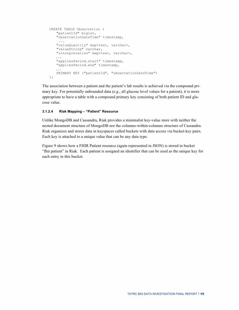
TATRC BIG DATA INVESTIGATION FINAL REPORT | 15
CREATE TABLE Observation ( "patientId" bigint, "observationDateTime" timestamp, ... "valueQuantity" map<text, varchar>, "valueString" varchar, "interpretation" map<text, varchar>, ... "appliesPeriod.start" timestamp, "appliesPeriod.end" timestamp, ... PRIMARY KEY ("patientId", "observationDateTime") );
The association between a patient and the patient’s lab results is achieved via the compound pri-mary key. For potentially unbounded data (e.g., all glucose level values for a patient), it is more appropriate to have a table with a compound primary key consisting of both patient ID and glu-cose value.
3.1.2.4 Riak Mapping – “Patient” Resource
Unlike MongoDB and Cassandra, Riak provides a minimalist key-value store with neither the nested document structure of MongoDB nor the columns-within-columns structure of Cassandra. Riak organizes and stores data in keyspaces called buckets with data access via bucket-key pairs. Each key is attached to a unique value that can be any data type.
Figure 9 shows how a FHIR Patient resource (again represented in JSON) is stored in bucket “fhir.patient” in Riak. Each patient is assigned an identifier that can be used as the unique key for each entry in this bucket.

TATRC BIG DATA INVESTIGATION FINAL REPORT | 16
Figure 9: Example of a FHIR Patient Resource Mapped to Riak
3.1.2.5 Riak Mapping – “Observation” Resource
The one-to-many relationship between patient and lab results proved to be problematic in Riak. We found that the basic key-value pair concept is not sufficient to support the type of queries re-quired by our tests. To resolve this deficiency, we opted to make use of Riak’s secondary indexes (referred to in the Riak documentation as 2i). However, Riak currently returns indexed query re-sults sorted in ascending order, whereas our use case is to retrieve the latest N records. That re-quires returning the entire list, and then pulling off the bottom N entries. Since the list is just the keys, the value for each element is short, but there may be hundreds or thousands of records for a patient. The solution was to combine the patient identifier (used as key in bucket “fhir.patient”) with the observation date and time of each lab result to first sort the secondary indexes by patient, then each set of lab results for that patient.
Figure 10 shows how a FHIR Observation resource is stored in bucket “fhir.observation” in Riak and its associated secondary index(es). The key for each entry key in this bucket is collected from the attribute “identifier.value” of the respective Observation resource.
{"resourceType":"Patient","identifier":[{"use":"secondary“, "label":"SSN“,
"system":"urn:oid:2.16.840.1.113883.4.1“, value":"416489606"},
{"use":"official", "label":"MRN", “system":"urn:oid:2.16.840.1.113883.3.198",
“value":"660896441","assigner":{"display":"Department of Defense"}}
],"name":[{"use":"official", “text":"Sellers, Steven J",
"family":["Sellers"], “given":["Steven","J"], “prefix":["Mr.“]}],"telecom":[{"system":"phone","value":"(269) 849-
2370","use":"home"},{"system":"phone","value":"(269) 849-
2370","use":"work"}],"gender":{
"coding":[{"system":"http://hl7.org/fhir/v3/AdministrativeGender","code":"M","display":"Male“}]},"birthDate":"1958-01-06T00:00:00-08:00","address":[{"use":"home","line":["4907 Lesmer Court","Apt # 85L"],"city":"Hamilton","state":"MI","zip":"49419","country":"US“
}],"active":true}
Key Value
660896441 {"resourceType":"Patient","identifier":[{"use":"secondary","label":"SSN","system":"urn:oid:2.16.840.1.113883.4.1","value":"416489606"},{"use":"official","label":"MRN","system":"urn:oid:2.16.840.1.113883.3.198","value":"660896441","assigner":{"display":"Department of Defense"}}],"name":[{"use":"official","text":"Sellers, Steven J","family":["Sellers"],"given":["Steven","J"],"prefix":["Mr."]}],"telecom":[{"system":"phone","value":"(269) 849-2370","use":"home"},{"system":"phone","value":"(269) 849-2370","use":"work"}],"gender":{"coding":[{"system":"http://hl7.org/fhir/v3/AdministrativeGender","code":"M","display":"Male"}]},"birthDate":"1958-01-06T00:00:00-08:00","address":[{"use":"home","line":["4907 Lesmer Court","Apt # 85L"],"city":"Hamilton","state":"MI","zip":"49419","country":"US"}],"active":true}
Bucket: fhir.patientFHIR Patient JSON Example

TATRC BIG DATA INVESTIGATION FINAL REPORT | 17
Figure 10: Example of a FHIR Observation Resource Mapped to Riak
3.2 Data Models
3.2.1 MongoDB
Figure 11 represents the MongoDB physical data model used in the experiments. It consists of a physical container, the “mongod” instance, at the top level. Within this container, a FHIR data-base was created to maintain a set of collections. Each collection provides storage for its respec-tive JSON documents as defined by the FHIR specification. For example, the “Patient” collection contains all the FHIR Patient resource documents.
{{"resourceType":"Observation","name":{“coding":[{"system":"http://loinc.org","code":"718-
7","display":"Hgb"}]
},"valueQuantity":{“value":9.0,“units":"g/dL","system":"http://unitsofmeasure.org","code":"g/dL“
},"issued":"2011-01-13T00:00:00-08:00","status":"final","identifier":{"use":"official","system":"urn:oid:2.16.840.1.113883.3.198","value":"1294982455907 CH 718-7","assigner":{"display":"Department of Defense"}
},"subject":{"reference":"Patient/187571512","display":"Driscoll Frazier"
}}
Key Value
1294982455907_CH_718-7
{"resourceType":"Observation","name":{"coding":[{"system":"http://loinc.org","code":"718-7","display":"Hgb"}]},"valueQuantity":{"value":9.0,"units":"g/dL","system":"http://unitsofmeasure.org","code":"g/dL"},"issued":"2011-01-13T00:00:00-08:00","status":"final","identifier":{"use":"official","system":"urn:oid:2.16.840.1.113883.3.198","value":"1294982455907 CH 718-7","assigner":{"display":"Department of Defense"}},"subject":{"reference":"Patient/187571512","display":"Driscoll Frazier"}}
Bucket: fhir.observationFHIR Observation JSON Example
2i Name 2i Value
ptid_obsdatetime187571512_2011-01-13T00:00:00-08:00
Secondary Indexes (2i)

TATRC BIG DATA INVESTIGATION FINAL REPORT | 18
Figure 11: MongoDB Physical Data Model
3.2.2 Cassandra
Figure 12 represents the Cassandra physical data model used in the experiments. The keyspace “fhir” is the physical structure holding a set of column families. Each column family (CF) is de-signed to store only data representative of a specific FHIR resource. For example, the “Patient” CF contains all the FHIR Patient resources.
Each row of a column family consists of a unique row key and columns of data of the same re-source type (see Figure 7 and Figure 8).

TATRC BIG DATA INVESTIGATION FINAL REPORT | 19
Figure 12: Cassandra Physical Data Model
3.2.3 Riak
Figure 13 represents the Riak physical data model used in the experiments. Riak has “pluggable” storage backends (e.g., BitCask and LevelDB) that provide flexibility in meeting operational needs. We used LevelDB because of its support for secondary indexes and its ability to accom-modate a large number of keys.
Each Riak Bucket is a container and virtual keyspace for Riak objects representing specific FHIR resource types. For example, all FHIR Patient resource objects are located in a Riak Bucket named “Patient” within keyspace “FHIR”.

TATRC BIG DATA INVESTIGATION FINAL REPORT | 20
Figure 13: Riak Physical Data Model
3.2.4 Neo4j
Figure 14 represents the Neo4j physical data model used in the experiments.

TATRC BIG DATA INVESTIGATION FINAL REPORT | 21
Figure 14: Neo4j Physical Data Model
3.3 Virtual Private Cloud
Testing was performed using virtual machines executing in the SEI’s Virtual Private Cloud (VPC). The VPC is an enclave within Amazon’s public Elastic Compute Cloud (EC2), configured as an extension of the SEI’s internal network. VPC virtual machines were used for both the data-base server instances as well as the YCSB client (described below). Virtual machines running in the VPC had access to the internet through the SEI proxy (i.e. egress), allowing easy download and installation of software packages, but were accessible only from the SEI internal network (i.e. no ingress).
All virtual machine instances used the EC2 “m1.large” instance type3. The characteristics of this instance type are:
• Instance Family: General purpose
• Processor Architecture: 64-bit
• Virtual CPUs: 2
• Memory: 7.5GiB
• Network Performance: Moderate
3 In early 2014, Amazon changed the instance types that they offered and although the m1.large type was desig-
nated “previous generation”, it was still available for use. We were about halfway through our experiments at that point, and continued to use the m1.large type exclusively for all of our instances.

TATRC BIG DATA INVESTIGATION FINAL REPORT | 22
All instances used “EBS (Elastic Block Store)-backed” storage for the root device. This decision was based on configuration of the the publically available Amazon Machine Image (AMI) as our base image.
All database server instances had two additional storage volumes: a 32GB volume used for data-base logs, and a 100GB volume used for database storage. These volumes were standard Amazon EBS volumes, and were not configured to use optimized input/output (Amazon “Provisioned IOPS” feature).
All instances used the CentOS 6.4 distribution.
3.4 Bulk Load
Kim Pham developed the specific bulk loader for each database, and performed the processing and measurement, and can provide additional information if needed.
To load the dataset required for our tests, custom Loader classes were developed for each NoSQL data store. These Java classes are responsible for parsing the respective CSV files and mapping the content of each CSV row into the appropriate vMR and/or FHIR resources. These resources are then inserted into the various NoSQL data stores using the following Java drivers:
• MongoDB: Spring MongoDB 1.1.0.RC1 bundled with MongoDB Java driver 2.7.1 version.
• Cassandra: Native Java driver version 1.0.2
• Riak: Protocol Buffers (Protobuffs) interface version 2.5.0
• Neo4j: Java API v2.1.4
A configuration file, loader.properties, is used in conjunction with the Loader classes to pass to each loader some common properties such as
• location and names of the CSV files,
• the number of client threads to run,
• which host(s) and port(s) to use for each cluster configuration,
• the amount of data to write to each data store, and
• how many times data will be replicated
The following is an example of a loader.properties file for loading lab results into a Riak bucket named fhir.observation:

TATRC BIG DATA INVESTIGATION FINAL REPORT | 23
# Location of CSV files dir_path=C:\\Workspaces\\TATRC\\SyntheticData\\samples\\R0.DS2\\ db_name=fhir db_user=tatrc db_pwd=bigdata # logging debug=true ### Riak host + port #db_host_uri=http://riak01.tatrc.net:8098/riak db_host=10.169.0.115 db_port=8087 ### Riak buckets + settings db_patient_table=fhir.patient db_observation_table=fhir.observation returnbody=false n_val=3 dw=quorum create_bucket=true ### Riak protocol to use, "pcb" or "http" riak_protocol=pcb cluster=true conn_pool_size=0 init_conn_pool_size=5 # connection timeout in millisec conn_ttl_millisec=1000 # idle connection timeout in millisec idle_conn_ttl_millisec=1000 # request timeout in millisec, 0 = no timeout request_ttl_millisec=0 # millisecs to pause between executions exec_wait_time=1 # number of client threads. If value = 0, threads count will be based on the # of cvs files. num_threads=4 # consistency level. 0=ANY, 1=ONE. write_consistency_level=0 # Data type to load load_patients=false load_labs=true load_meds=false load_allergies=false # List of CSV file names csv_files=Middlesex_HMO_Lab_Results_test.csv
When configured to run in multi-threaded mode, each thread will handle a fixed number of data sets based on this formula:
data set size / thread = total number of records in all CSV files / total number of threads
Bash scripts were developed to customize the parameters and execute the appropriate loader.
As an example, here is how the bulk loading of a single Cassandra node was accomplished:
• The bulk loader spawned five concurrent threads with each thread handling the loading of 500K rows of lab records.
• Each thread loaded its records in 50 batches, with 10,000 inserts per batch.
• Each thread paused for ten seconds between batches to prevent saturation of the CPU and memory on the Cassandra server. The pauses mitigated the effects of garbage collection (the delays could probably be fine-tuned to less than ten seconds).

TATRC BIG DATA INVESTIGATION FINAL REPORT | 24
• CPU and memory usage statistics for the server were captured with the pidstat command.
MongoDB data store characteristics:
• FHIR resources mapped to a MongoDB database “fhir” with collections “fhir.patient” and “fhir.labdata” of documents
• 1M MongoDB patient documents; average 1.3 KB per document
• 10M MongoDB lab result documents; average 1.5 KB per document
• 10M MongoDB medication documents; average 1.8 KB per document
• 52KMongoDB allergy data documents; average 1.0 KB per document
Cassandra data store characteristics:
• FHIR resources mapped to a Cassandra keyspace “fhir” with rows of column families “fhir.patient” and “fhir.labdata”
• 1M Cassandra rows of patient data; average 1.9 KB per row, 24 columns per row
• 10M Cassandra rows of lab data; average 1.1 KB per row, 14 columns per row
Riak data store characteristics
• FHIR resources mapped to Riak buckets “fhir.patient” and “fhir.observartion” of key-value pairs
• 1M values of patient data
• 10M values of lab data
Neo4j data store characteristics
• FHIR resources mapped to Neo4j graph nodes “Administrative” and “Clinical”
• 1M values of patient data
• 10M values of lab data
3.5 Read/Write Testing and Workloads
The test client for the read/write tests, and the related workload implementations, were developed by Chrisjan Matser, who can provide additional details if needed.
Our simulations are run using the Yahoo! Cloud Serving Benchmark4. This is a Yahoo! internal research project open-sourced in 2010 for the wider community to use [Cooper 2010]. It includes two main components:
1. a set of client interfaces to numerous popular cloud-based databases, including most of the ones we test in this report
2. a workload-generation and reporting framework.
4 https://github.com/brianfrankcooper/YCSB/

TATRC BIG DATA INVESTIGATION FINAL REPORT | 25
The client interface is specialized with custom code to ensure it correctly parses and loads the schema defined above, knows where the database is and how to login, and implements methods for doing scans (reads), inserts, updates, and deletes. The client code is installed on a machine in the VPC. Experiments consist of calling the YCSB client, passing it the custom data model code (e.g. Java code for loading patient data and querying Cassandra), and the number of threads to run. Thread counts measure concurrent database client sessions. In our tests this varied from 1-1000. This parameter allows us to simulate simultaneous connections (albeit from a single, CPU-limited IP address). Finally, YCSB specifies the type of experiment using a workload5 file. The following table shows some of the possible parameters:
Operation mix The proportion of operations that should be reads, updates, inserts or scans.
Database Parameters For each database, YCSB can (depending on the client interface) configure the DB response. For example, in MongoDB YCSB can ask for the read-preference to be Primary (read from the primary node – see below).
Distribution of records to select Zipfian or uniform; Zipfian is the default distribution Operation count Number of operations to perform. Available Ids A file that lists which Patient IDs to insert.
3.5.1 Workload Details
The main workload types (distinguished by the keyword at the end of the workload name) are shown in Table 3:
Table 3: Workload definitions for YCSB
Workload Name Workload Description readAll Read all records (up to 100) associated with that patient ID. No insert (write) operations. readLimit5Write Read up to 5 records for the given patient id (e.g. five lab results). Insert operations at
5%, reads 95%. readOnly1 No inserts, read only, but return at most one record. readWrite A mix of 95% reads and 5% inserts (writes). readWrite20 Mix is 80% reads, 20% writes.
We tested at most 20% writes. Our stakeholder kickoff meetings had determined a mix of 80% reads and 20% writes to be the more common use case.
Our experiments included the following workloads:
• Workloads run on the lab data:
− tatrc-lab-readAll − tatrc-lab-readLimit5Write − tatrc-lab-readOnly1 − tatrc-lab0readWrite − tatrc-lab-readWrite20 − tatrc-lab-delete
• Workloads on the other data:
− tatrc-pt-readAll-limit1
5 https://github.com/brianfrankcooper/YCSB/wiki/Core-Workloads

TATRC BIG DATA INVESTIGATION FINAL REPORT | 26
− tatrc-pt-readOne − tatrc-rx-readOnly
3.5.2 Running the Workloads
YCSB makes a distinction between the notions of “scan” and “read”.One can configure the pro-portion of operations in each test run with the variables scanproportion, writeproportion and read-proportion. When we started experiments with MongoDB we found two read methods: readOne() and read(). Besides the number of objects returned, they have different behaviour. readOne() will open a cursor, read a single object, close the cursor, return the object. read() will open a cursor and return it. You then have to iterate over the cursor to retrieve the objects. We decided to use the “readproportion” for the readOne() and commandeered the “scanproportion” for the read() tests where we return more than one object. This allowed us to compare the two different meth-ods.
Cassandra doesn't have this distinction, but we kept a similar approach. “read” property will read one object and “scan” will read up to “maxscanlength” objects. We set this to 100 for the “readAll” and 5 for the “readLimit5”. Note that the read/insert/delete operations are de-fined/customized in the YCSB client code.
We needed a reasonable collection of patient identifiers each time we ran the tests (which can in-volve close to a million operations at higher thread counts). We maintain a file of all available patient IDs (1,000,617 of them). This file gets loaded into memory. In order to select (at random) a given patient ID for the operation, we use the YCSB request distribution mode “Zipfian”. A Zipfian distribution is similar to a power-law distribution—the “long-tail”—so certain patient IDs have a higher probability of being selected, with the rest making up the long tail. This matches the expectation that certain patients will tend to make a disproportionate number of medical visits. For doing writes, we would start at "1000617" and increment by one.
In order to ‘prime’ the system, we would run a number of reads until there was reasonably con-sistent throughput. This allowed for the initial start-up effect to be excluded. Then, when doing runs, we would check the values for consistency with the primed system.
Finally, in order to delete the newly added records (synthetic records we no longer needed), we keep in memory a list of patient IDs that had an observation record inserted. At the end of the run, this is appended to a file called “insertedKeys”. When the write run completes, we run a “de-lete” run that pulls in all the insertedKeys, finds the corresponding observation record, and deletes it. We run the delete phase multi-threaded. Each thread will get a different ID to delete, delete it, then get the next ID to delete. The “insertedKeys” file is updated. Deleted IDs will be removed. At the end of a run assuming no errors, the “insertedKeys” file is empty.
3.6 Measurement Collection and Reporting
Detailed performance measurements were collected by the YCSB reporting framework. For each operation, YCSB measures the operation latency, which is the time from when the request is sent to the database until the response is received back from the database. The YCSB reporting framework records the minimum, maximum, and average operation latency separately for read and write operations.

TATRC BIG DATA INVESTIGATION FINAL REPORT | 27
The YCSB reporting framework also aggregates the latency measurements into histogram buck-ets, with separate histograms for read and write operations. There are 1001 buckets: the first bucket counts operations with latency from 0-999 microseconds, the second bucket counts opera-tions with latency from 1000-1999 microseconds, and so on up to bucket 999 which counts opera-tions with latency from 999,000-999,999 microseconds. The final “overflow” bucket counts oper-ations with latency greater than 1,000,000 microseconds (1 second). At the completion of the workload execution, the YCSB reporting framework calculates an approximation to the 95th per-centile and 99th percentile operation latency by scanning the histogram until 95% and 99% of the total operation count is reached, and then reporting the latency corresponding to that bucket where the threshold is crossed. There is no interpolation. If the overflow bucket contains more than 5% of the measurements, then the 95th percentile is reported as “0”, and if the overflow bucket con-tains more than 1% of the measurements, then the 99th percentile is reported as “0”.
We added a customization to the YCSB reporting framework to report Overall Throughput, in operations per second. This measurement was calculated by dividing the total number of opera-tions performed (read plus write) by the workload execution time. The execution time was meas-ured from the start of the first operation to the completion of the last operation in the workload execution, and did not include initial setup and final cleanup times. This execution time was also reported separately as Overall Run Time.
Each workload execution produced a separate output text file containing measurements and metadata. Metadata was produced by customizations to the YCSB reporting framework. The metadata included:
• The number of client threads
• The workload identifier
• The database cluster configuration (number of server nodes and IP addresses)
• Workload configuration parameters used for this execution
• The command line parameters used to invoke this execution
• Basic quality indicators (number of operations performed and number of operations com-pleted successfully).
• The time of day of the start and end of this execution.
The measurements were written by the standard YCSB reporting framework, using Javascript Object Notation (JSON) encoding.
For each database configuration tested, each workload was run three times. For each of these “runs”, the workload execution was repeated for each number of client threads (1, 2, 5, 10, 25, 50, 100, 200, 500, and 1000 client threads). This produced 30 separate output files (3 runs x 10 thread counts) for each workload. A data reduction program was developed to combine the measure-ments by averaging across the three runs for each thread count, and aggregating the results for all thread counts into a single file. The output of the data reduction program was a comma-separated variable (CSV) file that was structured to be easily cut and pasted into a Microsoft Excel spread-sheet template to produce the formatted tables and graphical plots. The details of the data analysis workflow are included below in Appendix B.

TATRC BIG DATA INVESTIGATION FINAL REPORT | 28
3.7 Network Partition Simulation
An important component of the iEHR environment is the presence of nodes (hospitals, clinics, etc) with limited or poor network connectivity. The clinical sites are operating on DoD networks that are a mix of DoD pipes and virtual networks running over the Internet. Some of the sites have as little as T1 bandwidth (1.54 Mbps, while most consumer plans offer 10-15 Mbps), shared for all IT needs, including PACS (Picture Archiving and Communications System, i.e., image trans-fers).
The issues are both throughput and latency—users are very sensitive to delays in reading and writing data using clinical applications like EHRs. We want to understand how NoSQL technolo-gies will work in the presence of network problems, i.e. latency problems, node failures, low bandwidth, and packet loss. There are two key questions. One, is there an effect on the database operations beyond that which is directly attributable to latency changes? Latency here refers sole-ly to network latency, and is not comparable to latency measured in YCSB. Two, are there any data integrity problems in a node-loss scenario? This is an important question, since a common tradeoff in NoSQL is strict consistency for availability. That is, NoSQL databases favor eventual consistency, so that the failure of a single node will not prevent writes from happening. Instead some form of global log is replicated, allowing failed nodes to re-sync with the history of the sys-tem. If a node fails, how much data is lost, and how long does it take the system to return to nor-mal operations?
Using our VPC capability, we constructed a sample network using some of these instances, and set up network simulations to reconstruct such problems. There are a number of tools that can simulate network problems: for example, netem and tc are tools that can force your internet connection into either thin, slow or lossy configurations.
We can perturb at least these variables:
• The client-data center connection or within datacenter. That is, tweak the client-db connec-tion or tweak the network bandwidth between db instances (in a replica).
• The numbers of data center nodes lost (and which). Losing a primary instance might be worse than a secondary, in a replica.
• Length of node loss. How long is the node down? Does it come back, and then need to re-synchronize the node list?
• Packet loss. How many (as a %)?
• Network delay (latency) or bandwidth (simulate with latency). We can add a throttle to make each packet take longer to leave the node (or arrive).
Here’s an example of applying traffic control (tc) and using ping on a VPC machine:

TATRC BIG DATA INVESTIGATION FINAL REPORT | 29
<ping> 8 packets transmitted, 8 received, 0% packet loss, time 7212ms rtt min/avg/max/mdev = 0.517/3.050/20.624/6.642 ms. tc qdisc change dev eth0 root netem delay 100ms 10ms 25% <ping> 25 packets transmitted, 25 received, 0% packet loss, time 24682ms rtt min/avg/max/mdev = 91.254/103.790/199.620/20.311 ms
The bold numbers show the difference after applying a 100ms delay, with 10ms variance 25% of the time: greater than three-fold increase in ping time (RTT).
The other tool we used was IPtables, which is a method for manipulating firewall rules. For example, the command iptables -I INPUT 1 -s 10.128.2.243 -j DROP will add a rule at position 1 on INPUT to drop all packets from the .243 IP. This simulates a node failure on this node. In a replicated database, that might mean messages synchronizing writes between primary and secondary don’t go through. In MongoDB, that triggers a rebalancing.
Results of these tests are presented in 4.2.

TATRC BIG DATA INVESTIGATION FINAL REPORT | 30
4 Results Discussion
We report results of evaluation of Read/Write Performance, Partition Tolerance, and Data Model Mapping for three database products: MongoDB version 2.2, a document store (http://docs.mongodb.org/v2.2/); Cassandra version 2.0, a wide column or column family store (http://www.datastax.com/documentation/cassandra/2.0); and Riak version 1.4, a key-value store (http://docs.basho.com/riak/1.4.10/).
We also tested Neo4J version 2.1.4, a graph database (http://neo4j.com/docs/2.1.4/), but that read/write performance testing was completed too late to be included in this report. The Neo4J scalability and replication for high availability are not sufficient to satisfy the iEHR requirements, so the results of those tests do not affect the conclusions presented below. Results of the Neo4J read/write testing are available from Chrisjan Matser.
4.1 Read/Write Performance Evaluation
Testing and measurement were performed on two database server configurations: Single node server, and a nine-node configuration that was representative of a possible production deploy-ment. The nine-node configuration used a topology that represented a geographically distributed deployment across three data centers. The data set was partitioned (i.e. “sharded”) across three nodes, and then replicated to two additional groups of three nodes each. This was achieved using MongoDB’s primary/secondary feature, and Cassandra’s data-center-aware distribution feature. The Riak features did not allow this “3x3” data distribution approach, and so we used a configura-tion where the data set was sharded across all nine nodes, with three replicas of each shard stored on the same nine nodes. For each configuration, we report results for the three workloads dis-cussed above.
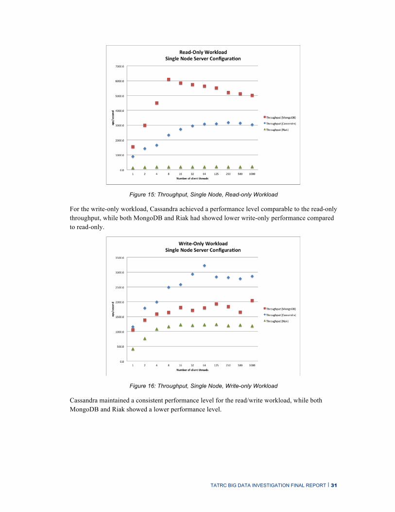
The single node server configuration is not viable for production use: There is only one copy of each record, causing access bottlenecks that limit performance and a single point of failure limit-ing availability. However, this configuration provides some insights into the basic capabilities of each of the products tested. The throughput, in operations per second, is shown for each of the three workloads in Figure 15 - Figure 17: read-only, write-only, and read-write.
For the read-only workload, MongoDB achieved very high performance compared to Cassandra and Riak, due to MongoDB’s indexing features that allowed the most recent observation record to be accessed directly, while Cassandra returned all observations for the selected patient back to the client where the most recent record was selected from the result set. Riak’s relatively poor per-formance is due to an internal architecture that is not intended for deployment on a single node, as multiple instances of the storage backend (in our case, LevelDB) compete for disk I/O.
TATRC BIG DATA INVESTIGATION FINAL REPORT | 31
Figure 15: Throughput, Single Node, Read-only Workload
For the write-only workload, Cassandra achieved a performance level comparable to the read-only throughput, while both MongoDB and Riak had showed lower write-only performance compared to read-only.
Figure 16: Throughput, Single Node, Write-only Workload
Cassandra maintained a consistent performance level for the read/write workload, while both MongoDB and Riak showed a lower performance level.

TATRC BIG DATA INVESTIGATION FINAL REPORT | 32
Figure 17: Throughput, Single Node, Read/Write Workload
For the read/write workload, the average latency and 95th percentile latency is shown in Figure 18 for read operations and in Figure 19 for write operations. In both cases the average latency for both MongoDB and Riak increases as the number of concurrent client sessions increases.
Figure 18: Read Latency, Single Node, Read/Write Workload

TATRC BIG DATA INVESTIGATION FINAL REPORT | 33
Figure 19: Write Latency, Single Node, Read/Write Workload
Our testing varied the number of test client threads (or equivalently, the number of concurrent client sessions) from one up to 1000. Increasing the number of concurrent client sessions stresses the database server in several ways. There is an increase in network I/O and associated resource utilization (i.e. sockets and worker threads). There is also an increase in request rate, which in-creases utilization of memory, disk I/O, and other resources. The results in Figure 15 - Figure 17 show that server throughput increases with increased load, up to a point where I/O or resource utilization becomes saturated, and then performance remains flat as the load is increased further (for example, Cassandra performance at 64 concurrent sessions in Figure 17), or decreases slight-ly, probably due to competition for resources within the server (for example, MongoDB perfor-mance at eight concurrent sessions in Figure 17).
Operating with a large number of concurrent database client sessions is not typical for a NoSQL database. A typical NoSQL reference architecture has clients connecting first to a web server tier and/or an application server tier, which aggregates the client operations on the database using a pool of perhaps 16-64 concurrent sessions. However, our prototyping was in support of the mod-ernization of the AHLTA system that used thick clients with direct database connections, and so the IPO wanted to understand the implications of retaining that thick client architecture.
In the nine-node configuration, we had to make several design decisions to define our representa-tive production configuration. The first decision was how to distribute client connections across the server nodes. MongoDB uses a centralized router node, and all clients connected to the single router node. Cassandra’s data center aware distribution feature created three sub-clusters of three nodes each, and client connections were spread uniformly across the three nodes in one of the sub-clusters. In the case of Riak, client connections were spread uniformly across the full set of nine nodes.
Another design decision was how to achieve strong consistency, which requires defining both write operation settings and read operation settings [Gorton 2014]. Each of the three databases offered slightly different options. The selected options are summarized in Table 4, with the details
TATRC BIG DATA INVESTIGATION FINAL REPORT | 34
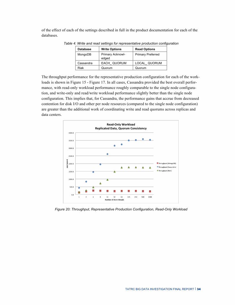
of the effect of each of the settings described in full in the product documentation for each of the databases.
Table 4: Write and read settings for representative production configuration Database Write Options Read Options MongoDB Primary Acknowl-
edged Primary Preferred
Cassandra EACH_ QUORUM LOCAL_ QUORUM Riak Quorum Quorum
The throughput performance for the representative production configuration for each of the work-loads is shown in Figure 15 - Figure 17. In all cases, Cassandra provided the best overall perfor-mance, with read-only workload performance roughly comparable to the single node configura-tion, and write-only and read/write workload performance slightly better than the single node configuration. This implies that, for Cassandra, the performance gains that accrue from decreased contention for disk I/O and other per node resources (compared to the single node configuration) are greater than the additional work of coordinating write and read quorums across replicas and data centers.
Figure 20: Throughput, Representative Production Configuration, Read-Only Workload

TATRC BIG DATA INVESTIGATION FINAL REPORT | 35
Figure 21: Throughput, Representative Production Configuration, Write-Only Workload
Figure 22: Throughput, Representative Production Configuration, Read/Write Workload
Riak performance in this representative production configuration is better than the single node configuration. In test runs using the write-only workload and the read/write workload, our test client had insufficient socket resources to execute the workload for 500 and 1000 concurrent ses-sions. These data points are reported as zero values in Figure 24 and Figure 26. We later deter-mined that this resource exhaustion was due to an ambiguous description of Riak’s internal thread pool configuration parameter, which creates a pool for each client session and not a pool shared by all client sessions. After determining that this did not impact the results for one through 250 concurrent sessions, and given that Riak had qualitative capability gaps with respect to our strong consistency requirements (as discussed below), we decided not to re-execute the tests for those data points.

TATRC BIG DATA INVESTIGATION FINAL REPORT | 36
MongoDB performance is significantly worse here than the single node configuration. Two fac-tors influenced the MongoDB results. First, the representative production configuration is shard-ed, which introduces the router and configuration nodes into the MongoDB deployment architec-ture. The router node directs each request to the appropriate shard, based on key mapping information contained in the configuration node. Our tests ran with a single router node, which became a performance bottleneck. Figure 25 and Figure 26 show read and write operation latency for the read/write workload, with nearly constant average latency for MongoDB as the number of concurrent sessions is increased, which we attribute to saturation of the rapid saturation of the router node.
Figure 23: Read Latency, Representative Production Configuration, Read/Write Workload
Figure 24: Write Latency, Representative Production Configuration, Read/Write Workload

TATRC BIG DATA INVESTIGATION FINAL REPORT | 37
The second factor affecting MongoDB performance is the interaction between the sharding scheme used by MongoDB and the write-only and read/write workloads that we used, which was discovered near the end of our testing. Both Cassandra and Riak use a hash-based sharding scheme, which provides a uniformly distributed mapping from the range of keys onto the physical nodes. In contrast, MongoDB uses a range-based sharding scheme with rebalancing (http://docs.mongodb.org/v2.2/core/sharded-clusters/). Our write-only and read/write workloads generated a monotonically increasing sequential key for new records to be written, which caused all write operations to be directed to the same shard, since all of the write keys mapped into the space stored in that shard. This key generation approach is typical (in fact, many SQL databases have “autoincrement” key types that do this automatically), but in this case, it concentrates the write load for all new records in a single node and thus negatively impacts performance.
Figure 25: Read Latency, Representative Production Configuration, Read/Write Workload
Figure 26: Write Latency, Representative Production Configuration, Read/Write Workload

TATRC BIG DATA INVESTIGATION FINAL REPORT | 38
Finally we report transaction performance results that quantify the performance cost of strong replica consistency. These tests were limited to the Cassandra and Riak databases – the perfor-mance of MongoDB in the representative production configuration was such that no additional characterization of that database was warranted for our application. These tests used a combina-tion of write operation settings and read operation settings that resulted in eventual consistency, rather than the strong consistency settings used in the tests described above. Again, each of the three databases offered slightly different options. The selected options are summarized in Table 5, with the details of the effect of each of the settings described in full in the product documentation for each of the databases.
Table 5: Write and read settings for eventual consistency configuration Database Write Options Read Options Cassandra ONE ONE Riak noquorum noquorum
Figure 27 shows throughput performance for the read/write workload on the Cassandra database, comparing the representative production configuration with the eventual consistency configura-tion. For any particular number of concurrent client sessions, the eventual consistency configura-tion provides higher throughput, and the eventual consistency configuration throughput flattens out at a higher level than strong consistency.
The same comparison is shown for the Riak database, in Figure 28. Here, the difference in throughput between the strong consistency configuration and the eventual consistency configura-tion is much less obvious. As discussed above, test client configuration issues resulted in no data recorded for 500 and 1000 concurrent sessions.
Figure 27: Cassandra – Comparison of strong consistency and eventual consistency
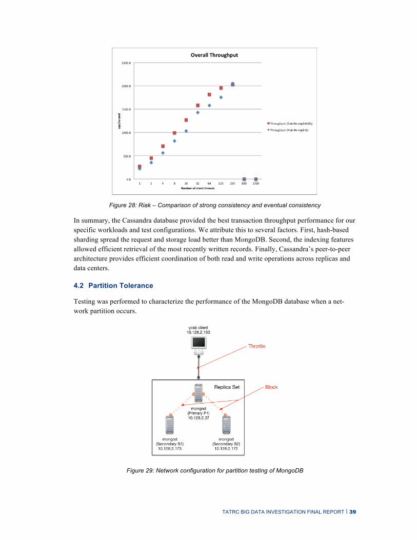
TATRC BIG DATA INVESTIGATION FINAL REPORT | 39
Figure 28: Riak – Comparison of strong consistency and eventual consistency
In summary, the Cassandra database provided the best transaction throughput performance for our specific workloads and test configurations. We attribute this to several factors. First, hash-based sharding spread the request and storage load better than MongoDB. Second, the indexing features allowed efficient retrieval of the most recently written records. Finally, Cassandra’s peer-to-peer architecture provides efficient coordination of both read and write operations across replicas and data centers.
4.2 Partition Tolerance
Testing was performed to characterize the performance of the MongoDB database when a net-work partition occurs.
Figure 29: Network configuration for partition testing of MongoDB

TATRC BIG DATA INVESTIGATION FINAL REPORT | 40
Our network configuration for MongoDB is shown in Figure 29. We can also configure Mon-goDB with different settings for read preference (what node can be read from) and write concern (as described in the MongoDB product documentation), or how important it is that our recent write operation is stored on all nodes in the replica. In these experiments we used read preference of primary and write concerns of both acknowledged (Figure 30) and replica acknowledged6, where the data must first be written to the replica prior to the write being acknowledged to the client.
Figure 30: MongoDB “acknowledged” write concern
We conducted the experiments only on MongoDB, and report here on the read-write scenarios with 80% reads. Our baseline was a series of workloads run with no network perturbations delib-erately introduced, and although Amazon’s network topology is naturally subject to the stochastic changes inherent in the wider Internet, we did not observe any major disturbances. Our second run (no-ack) introduced some node loss at random intervals, and our third run (ack) introduced similar stochastic node loss using a write concern of ‘secondary acknowledged’. We observed obvious short-term spikes in the last two runs, but this is likely due to the Java garbage collector being activated. There was no clear causal relationship between a node failing, and subsequent through-put problems. However, as can be seen in Figure 31, there were clear overhead burdens in moving to this level of consistency guarantee. Furthermore, there are large numbers of exceptions that must be handled because the connection in the Mongo client does not handle them by default, and cannot detect a problem until invoked.7 For example, in the no-ack scenario, we do not have any faults detected doing a write operation, while in the ack scenario, between 17% and 34% of writes would fail, due to the node loss.
6 http://docs.mongodb.org/manual/core/replica-set-write-concern/
7 http://stackoverflow.com/questions/18564607/com-mongodb-dbportpool-goterror-warning-emptying-dbportpool-to-ip27017-b-c-of

TATRC BIG DATA INVESTIGATION FINAL REPORT | 41
Figure 31: Impact of partition on MongoDB insert operation latency
We also examined the results of throttling the bandwidth with respect to a high bandwidth situa-tion. Using the tc tool, we applied throttling to simulate latency on the network of +100 ms 25% autocorrelated with +/- 10% variance. As expected, this also slows down the throughput of our MongoDB client, as shown in Figure 32 (higher is better). By 250 threads, however, the concur-rency of the threads has overwhelmed our network link in both cases, resulting in a very similar performance.
Figure 32: Impact of network latency on MongoDB insert operation throughput
Finally, we investigated the possibility of data loss. If writes are not acknowledged by the repli-cas, there is a chance of records being overwritten when a node that went down is brought back online. We recorded the number of records written on all three nodes, as well as the timestamps of the oplog, the central data structure for ensuring consistency in MongoDB. We could not see any major differences in these values, and in particular, the number of nodes was the same in all three scenarios. For example, a result like:
37: optime=Timestamp(1411011459, 11) records: 5084075 173: optime=Timestamp(1411011459, 18) records: 5084075
tells us that the primary, node 37, has the same number of records as the secondary.
Our conclusions from the latency/consistency experiments in MongoDB was that the database performed as expected, handling node loss gracefully. However, the large number of exceptions generated in a high-consistency (secondary acknowledge) scenario puts a large burden on the pro-grammer to determine correct behavior (likely to re-send the data).

TATRC BIG DATA INVESTIGATION FINAL REPORT | 42
4.3 Bulk Load
4.3.1 MongoDB
4.3.1.1 Insert-Method Performance
MongoDB driver supports two types of write: serial insert and bulk insert where each document is inserted atomically. MongoDB also has two modes of index; foreground (default) and back-ground index operations.
We ran a number of test cases to determine if one method of insert and indexing is better than the other by inserting batches of 400,000 vMR documents.
The test cases were first run without index on the patientId field and then with ascending index on the patientId field using both foreground and background indexing methods. A find operation on the patientId field with consistent # of results was performed after every batch writes.
We found that serial write operations are capable of inserting 1/3 more records per second than the “bulk” write operations regardless of indexing as shown by the metrics collected in Table 6 and
Table 7. Neither method of indexing yielded better results than the other.
Table 6: Bulk Write performance for each batch of 400K records. Collection Count
Bulk Write without index (sec)
Bulk Write with fore-ground indexing (sec)
Bulk Write with background indexing (sec)
400,000 170.6 173.5 177.4 800,000 164.8 163.0 163.0 1,200,000 150.1 157.0 151.6 1,600,000 130.6 167.3 167.7 2,000,000 157.3 174.4 147.8 2,400,000 162.4 171.3 153.9 2,800,000 156.0 165.9 160.4 3,200,000 115.6 157.1 154.0 3,600,000 151.6 156.8 161.9 4,000,000 150.1 160.6 161.5 4,400,000 165.7 160.0 157.3 4,800,000 181.7 170.5 167.9

TATRC BIG DATA INVESTIGATION FINAL REPORT | 43
Table 7: Serial Write performance for each batch of 400K records. Collection Count
Serial Write without in-dex (seconds)
Serial Write with fore-ground indexing (se-conds)
Serial Write with background indexing (seconds)
400,000 111.0 110.6 110.8 800,000 108.0 109.6 109.0 1,200,000 105.0 113.7 117.9 1,600,000 94.0 105.0 106.0 2,000,000 105.7 106.2 108.8 2,400,000 97.1 121.6 112.4 2,800,000 100.6 122.3 120.0 3,200,000 106.8 109.9 103.2 3,600,000 104.5 125.1 113.6 4,000,000 100.4 122.5 115.3 4,400,000 106.1 112.8 109.0 4,800,000 114.3 130.7 122.1
After every insert, update, or delete operation, MongoDB must update every index associated with the collection in addition to the data itself. Therefore, every index on a collection adds some amount of overhead for the performance of write operations. However, looking at the data col-lected in Table 1 that overhead seemed negligible.
4.3.1.2 Effect of Insert Method on Read Performance
The first read request takes more time for both indexed and non-indexed fields as shown below in Table 8 and
Table 9. With indexing, read results can take as low as 8 millisecs to complete while performanc-es of read without indexing degraded as the size of the collection grew. This is because non-indexed queries do a lot of disk reads.
Table 8: Read performances after inserting each batch of 400K records.
Collection Count Non-Index Field Read (millisecs) * Non-Index Field Read (millisecs) ** 400,000 786 775 800,000 1,294 1,420 1,200,000 5,175 2,046 1,600,000 4,928 2,833 2,000,000 2,706 2,850 2,400,000 3,497 5,305 2,800,000 3,283 3,569 3,200,000 4,235 5,387 3,600,000 4,089 6,014 4,000,000 4,852 4,918 4,400,000 5,686 5,706 4,800,000 30,614 25,815

TATRC BIG DATA INVESTIGATION FINAL REPORT | 44
Table 9: Read performances after inserting each batch of 400K records. Collection Count
Foreground Index Field Read (mil-lisecs) *
Foreground Index Field Read (mil-lisecs) **
Background Index Field Read (mil-lisecs) *
Background Index Field Read (millisecs) **
400,000 29 29 32 28 800,000 15 12 21 11 1,200,000 12 13 12 13 1,600,000 15 15 15 12 2,000,000 10 15 13 17 2,400,000 10 8 23 12 2,800,000 8 17 8 13 3,200,000 9 13 8 15 3,600,000 8 14 7 15 4,000,000 11 15 9 12 4,400,000 8 18 8 14 4,800,000 11 14 11 14
Notes:
* after Bulk Write operations
** after Serial Write operations
4.3.2 Cassandra
Figure 33 shows the Cassandra bulk-load performance for batch inserts executed by increasing numbers of threads.
Figure 33: Bulk load latency vs threads

TATRC BIG DATA INVESTIGATION FINAL REPORT | 45
4.3.3 Riak
Initial results of bulk load operations using the Riak HTTP API yielded extremely slow perfor-mances so we switched to the native Protocol Buffers API.
Table 10shows the result of the bulk load of data into the “Observation” bucket. This bucket was configured with the following settings on its properties prior to starting the load process:
• w = 0 (The number of replicas which must reply to a write request, indicating that the write was received.)
• dw = 0 (The number of replicas which must reply to a write request indicating that the write was committed to durable storage for the write to be deemed successful.)
This will effectively throw data into the Riak cluster as fast as possible and not care if the write succeeds.
Table 10: Bulk load performances for bucket “Observation”
# of Threads Avg Latency (sec/thread)
Avg Throughput (ops/sec) # of Ops/Thread Failed Ops
1 4,454 449 1,999,997 0
2 2,450 816 1,000,000 0
4 1,668 1,199 500,000 0
8 1,617 1,237 250,000 0
16 1,548 1,292 125,000 0
32 1,605 1,246 62,500 0
64 1,492 1,340 31,250 0
128 1,494 1,339 15,625 0
256 1,495 1,338 7,813 0
512 1,399 1,430 3,906 0
1024 973 2,055 1,953 80
Figure 34 shows the bulk load performance of Riak.

TATRC BIG DATA INVESTIGATION FINAL REPORT | 46
Figure 34: Bulk load latency vs operations
4.3.4 Neo4j
Initial attempts at inserting data into a Neo4j instance running in server mode used a Neo4j JDBC driver. This driver provides access to standard JDBC interfaces while wrapping the Neo4j REST protocol underneath. This resulted in extremely poor performances due to the overhead incurred with network and transaction management.
We switched to running the Neo4j instance in embedded mode to allow us to use the Neo4j Core API, which has higher performance and no network management overhead. We also confirmed that after data is loaded into an embedded Neo4j data store it can be re-configured to serve as the data store for a stand-alone Neo4j (server mode).
The data model (see Figure 13) designed for our experiments required the load process to look up a “Patient” node in the graph so that a relationship can be created when creating a new Observa-tion node. This functionality, retrieve a node by its property, is only supported when the Neo4j embedded data store is opened in transactional mode. However, transactional mode has inherent performance costs and was found to add as much as 100 msec to the processing of a group of transactions. On a million-node insertion this can translate into an additional 28 hours.
To further optimize the bulk load process, the workflows of the data loader were modified to
• Open the Neo4j embedded data store in non-transactional mode using the Neo4j BatchInserters utility. This utility bypasses transactions and other checks and can only be used on an embedded Neo4j data store as it is not thread safe.

TATRC BIG DATA INVESTIGATION FINAL REPORT | 47
• After each Patient node is created, its Neo4j node id is saved to a temporary file which can then be used during the loading of the Lab Results dataset.
• When creating an Observation node, the relevant Patient node id is retrieved in order to cre-ate the SUBJECT relationship between the new Observation node and the existing Patient node.
Overall, loading and creating 1,000,617 Patient nodes took approximately 7 min 45 sec while the ten million lab results took approx 1 hr 15 min from start to end. On average it took less than 1 msec per node.
4.4 Data Model Fit/Mapping
Throughout the prototype design and development, we developed a set of findings that are quali-tative. Here we report on these qualitative findings in the area of alignment of our data model with the capabilities provided by each database.
The most significant data modeling challenge was the representation of the one-to-many relation from patient to lab results, coupled with the need to efficiently access the most-recently written lab results for a particular patient.
Zola has analyzed the various approaches and tradeoffs of representing the one-to-many relation in MongoDB [Zola 2014]. We used a composite index of (Patient ID, Observation ID) for lab result records, and also indexed by the lab result date-time stamp. This allowed efficient retrieval of the most recent lab result records for a particular patient.
A similar approach was used for Cassandra. Here we used a composite index of (PatientID, lab result date-time stamp). This caused the result set returned by the query to be ordered, making it efficient to find and filter the most recent lab records for a particular patient. Cassandra 2.0, which was released after our testing was completed, offers the ability to iterate over the result set, return-ing only one record at a time to the client, which may provide additional efficiency improvements.
Representing the one-to-many relation in Riak was more complicated. Riak’s basic capability is retrieval of a value, given a unique key. The peer-to-peer gossip protocol ensures that every node in the cluster can map from a record’s key to the node (or nodes, if data is replicated) that holds the record. Riak also provides a “secondary index” capability that allows record retrieval when the key is not known, however each server node in the cluster stores only the indexes for the portion of the records that are managed by the node. When an operation requests all records with a partic-ular secondary index value, the request coordinator must perform a “scatter-gather”, asking stor-age node for records with the desired secondary index value, waiting for all nodes to respond, and then sending the list of keys back to the requester. The requester must then make a second data-base request with the list of keys, in order to retrieve the record values. The latency of the “scat-ter-gather” to locate records, and the need for two request/response round trips had a negative im-pact on Riak’s performance for our data model. Furthermore, there is no mechanism for the server to filter and return only the most recent observations for a patient. All observations must be re-turned to the client, and then sorted and filtered. We attempted to de-normalize further, by intro-ducing a data set where each record contained a list of the most recently written observations for each patient. However, this required an atomic read-modify-write of that list every time a new observation is added for the patient, and that capability was not supported in Riak 1.4.

TATRC BIG DATA INVESTIGATION FINAL REPORT | 48
Objectively, MongoDB and Cassandra both provided a relatively straight-forward data model mapping and both provided the strong consistency needed for our customer’s EHR application. Subjectively, the data model mapping in MongoDB was more transparent than the use of the Cas-sandra Query Language (CQL), and the indexing capabilities of MongoDB were a better fit for this application.
4.5 Limitations
As noted above, the results in this report, although detailed and quantitative, are not intended to be used to make a final technology selection for any system. The results should be used to narrow the solution space to allow focus on analysis and further testing of a small number of candidates. There are a number of specific limitations to generalizing these results that we highlight here.
4.5.1 Environment/Optimization
The prototyping and measurements were performed using virtual machines in a cloud computing environment. Virtualization of computing and storage resources may impact performance differ-ently for different NoSQL products.
In the cases where product documentation provided recommendations for configuration, we fol-lowed those recommendations. We did not perform additional tuning of memory, network and storage I/O, or other virtual machine or operating system parameters.
We used standard EC2 Elastic Block Store (EBS) devices for storage of database data files and log files. We did not use the EC2 Provisioned I/O (i.e. “IOPS”) feature.
4.5.2 Scope/Coverage of Use Cases
The prototyping focused on a limited number of workloads that represented the core EHR use cases. Other workloads corresponding to other use cases may produce different results.
4.5.3 Caching
The workloads that we used did not generally make repeated retrieval of the same records, so most reads required disk access rather than retrieving cached values. Caching would typically im-prove performance.
4.5.4 Data Set Size
Our data set was limited to approximately one million patient records and 10 million observation records. This is a relatively small fraction of the actual MHS EHR workload. The workloads we used performed queries on indexed fields rather than full table scans, so the results presented here should not change with increased data set size. However, as the data set grows, different configu-ration (i.e. sharding configuration) would likely be necessary.
4.5.5 Test Client Limits
We used a single VPC instance running YCSB as our test client. Our results indicate that the measurements were not limited by client performance, however an environment with multiple client systems could certainly produce a higher load on the database, which might change results.

TATRC BIG DATA INVESTIGATION FINAL REPORT | 49
4.5.6 Polyglot Persistence
We used a single database for both patient and observation records. We did not study the use of polyglot persistence, which is a common architecture pattern in NoSQL systems [Sadalage 2012]. Polyglot persistence stores different types of records in different databases, with the database se-lected to match the data model, indexing and query workload, and other quality attribute require-ments of the system. For example, patient records might be stored in a key-value database such as Riak, while observation records might be stored in a document database such as MongoDB.

TATRC BIG DATA INVESTIGATION FINAL REPORT | 50
5 Conclusion
NoSQL database technology offers benefits of scalability and availability through horizontal scal-ing, replication, and simplified data models, but the specific implementation must be chosen early in the architecture design process. We have described a systematic method to perform this tech-nology selection in a context where the solution space is broad and changing fast, and the system requirements may not be fully defined. Our method evaluates the products in the specific context of use, starting with elicitation of quality attribute scenarios to capture key architecture drivers and selection criteria. Next, product documentation is surveyed to identify viable candidate tech-nologies, and finally, rigorous prototyping and measurement is performed on a small number of candidates to collect data to make the final selection.
We described the execution of this method to evaluate NoSQL technologies for an electronic healthcare record system, and presented the results of our measurements of transactional perfor-mance and partition tolerance, along with a qualitative assessment of alignment of the NoSQL data model with system-specific requirements. We presented lessons learned from our application of the selection method, and from our execution of the prototyping and measurements.
We have identified the benefits of having a trusted knowledge base that can be queried to discover the features and capabilities of particular NoSQL products, and accelerate the initial screening to identify viable candidate products for a particular set of quality attribute scenario requirements. This is an area for further research. Additionally, our testing of network partitions required manu-al intervention, and further research to automate the triggering of partitions and measurement col-lection is needed.
5.1 Lessons Learned
We separate our lessons learned into two broad categories. The first category pertains to the over-all technology selection process for the storage layer in a big data system, and the second category pertains to the development and execution of the prototyping and measurement.
5.1.1 Technology Selection Process
In big data systems using NoSQL technology, there is a coupling of concerns between the select-ed storage layer product, the deployment topology, and the application architecture [Gorton 2014]. Technology selection is an architecture decision that must be made early in the design cy-cle, and is difficult and expensive to change. The selection must be made in a setting where the problem space definition may be incomplete, and the solution space is large and rapidly changing as the open source landscape continues to evolve.
We found it helpful to employ a process that considers the candidate technology in the context of use. In the case of NoSQL and big data systems, the context of use includes characterizing the size and growth rate of the data (number of records and record size), the complexity of the data model along with concrete of key relations and navigations, operational environment including system management practices and tools, and user access patterns including operation mix, queries, and number of concurrent users.

TATRC BIG DATA INVESTIGATION FINAL REPORT | 51
We found the use of quality attribute scenarios [Barbacci 2003] to be helpful to assist stakeholders to concretely define selection criteria. After eliciting a number of scenarios of interest to one or more stakeholders, we were able to cluster and prioritize the scenarios to identify “go/no-go” cri-teria – the capabilities that the selected technology must have, or behaviors or features that, if pre-sent in a product, disqualify it from use in the system. These criteria may be quantitative or quali-tative. In the case of quantitative criteria, there may be hard thresholds that must be met, but this type of criterion can be problematic to validate, since there are a large number of infrastructure, operating system, database product, and test client parameters that can be tuned in combination to impact absolute performance (and certainly, a final architecture design must include that tuning). It can be more useful for product selection to frame the criterion in terms of concerns about the shape of the performance curve: for example, does throughput increase linearly with load up to some level where throughput flattens out, and is that point of flattening within our range of inter-est? Understanding the sensitivities and trade offs in a product’s capabilities may be sufficient to make a selection, and also provides valuable information to make downstream architecture design decisions regarding the selected product.
We used this context of use definition to perform a manual survey of product documentation to identify viable candidate products. As this was our first time working with NoSQL technology, the manual survey process was slow and inefficient. We began to collect and aggregate product feature and capability information into a queryable, reusable knowledge base, which included general quality attribute scenarios as templates for concrete scenarios, and linked the quality at-tribute scenarios to particular product implementations and features. This knowledge base was used successfully for later projects, and is an area for further research.
The selection process must balance cost (in time and resources) with fidelity and measurement precision. The solution space is changing rapidly. During the course of our evaluation, each of the candidate products released at least one new version that included changes to relevant features, so a lengthy evaluation process is likely to produce results that are not relevant or valid. Further-more, if a cloud infrastructure is used to support the prototyping and measurement, then changes to that environment can impact results. For example, during our testing process, Amazon changed standard instance types offered in EC2. Our prototypes all used the instance type “m1.large”, which was eliminated as a standard offering during our testing, but we were still able to use it as a “legacy instance type” until completion of our tests. Our recommendation is to perform prototyp-ing and measurement for just two or three products, in order to complete quickly and deliver valid and relevant results.
To maintain urgency and forward progress while defining the selection criteria and performing the prototyping and measurement, we found it useful to ask, “How will knowing the answer to this question change the final selection decision?” In many cases, the answer would be needed to make downstream design decisions of the particular product was to be used in the system, but the answer was not necessary to make a selection decision, and so that measurement was put off until an appropriate time later in the design process.
5.1.2 Prototyping and Measurement
We started our prototyping and measurement using a cloud infrastructure, which proved to be essential for efficient management and execution of the tests. Although our initial test was a sin-gle server and single client, we quickly grew to product configurations with more than 10 servers,

TATRC BIG DATA INVESTIGATION FINAL REPORT | 52
and were frequently executing on more than one product configuration at a time. Our peak utiliza-tion was over 50 concurrently executing server nodes (divided across several product configura-tions), which is more than can be efficiently managed in most physical hardware environments.
We had a continual tension between using manual processes for server deployment and manage-ment, and automating some or all of these processes. Repeating manual tasks conflicts with soft-ware engineering best practices such as “don’t repeat yourself”8, but in retrospect we think that the decision to always make slow forward progress, rather than stopping to automate, was appro-priate. Organizations that already have a proven automation capability and expertise in place may reach a different conclusion. We did develop simple scripts to automate test execution and most of the data collection, processing, and visualization. These tasks were performed frequently, had many steps, and needed to be repeatable.
We started evaluating each product using a single server configuration, which validated the soft-ware installation and configuration, and allowed easier debugging of the test client. Recognize that some NoSQL products (e.g., Riak) are not designed to operate well in this configuration, and so this configuration may not produce any useful test results. We next expanded our configuration to partition (“shard”) the data set across multiple nodes, which allowed us to validate the cluster configuration. Finally, we introduced data replication into the test configuration. We found this sequence to be effective, providing confidence in the validity of the measurements.
Our context of use and workloads required that the database was populated with a complete data set. We found that bulk load is a special type of workload, and each database product had specific recommendations and special APIs for this function. In some cases (i.e. MongoDB), recommen-dations like “pre-splitting” the data set simply improved bulk load performance. In other cases, we found that following the recommendations was necessary to avoid failures due to resource exhaustion in the database server. We recommend that if bulk load is not one of your selection criteria, then take a brute force approach to load the data, and then use database backups, or virtu-al machine or storage volume snapshots to return to the initial state as needed.
All of our tests that performed write operations ended the test by restoring the database to its ini-tial state. We found that deleting records in most NoSQL databases is very slow, taking as much as 10 times longer than a read or write operation. In retrospect, we would consider using snap-shots to restore state, rather than cleaning up using delete operations.
It is critical that you understand your measurement framework. Although YCSB has become the de facto standard for NoSQL database characterization, the 95th and 99th percentile measurements that it reports are only valid under certain latency conditions, as we discussed above. The YCSB implementation could be modified to extend the validity of those measurements to a broader range of latencies, or alternative metrics can be used for selection criteria.
8 http://c2.com/cgi/wiki?DontRepeatYourself

TATRC BIG DATA INVESTIGATION FINAL REPORT | 53
Appendix A – Scenarios Developed in Stakeholder Workshop
The following quality attribute scenarios were discussed during the workshop. Each scenario is expressed in the form of stimulus, environment, response [Barbacci 2003].
1. A patient with a scheduled appointment arrives at an MTF. The MTF has good WAN bandwidth and connectivity. The clinician’s EHR application displays complete patient healthcare information within milliseconds of a request for it.
Notes: “Good WAN bandwidth and connectivity” must be defined to completely specify this sce-nario. “Complete patient healthcare information” for an outpatient encounter includes (at least) all information related to the previous 10 patient encounters.
2. A patient with no scheduled appointment arrives at an MTF with 9 other unscheduled patients. The MTF has good WAN bandwidth and connectivity. The patient check-in initiates a request for the patient’s EHR, and a clinician’s EHR application displays complete patient healthcare information within 5 minutes of the initial request.
3. Several clinicians see a patient during an encounter, and each makes an entry in the patient’s EHR (e.g., a technician takes and records vital signs, a nurse takes problem and history, a physician examines patient and makes diagnosis, etc.). Each clinician may use a different input device or instance of the EHR application. The data entered by one clinician is immediately visible to other clinicians viewing the patient’s EHR.
4. A patient with no scheduled appointment arrives at an MTF. The MTF has good WAN bandwidth and connectivity. A clinician needing to see images from a previous encounter with the patient is able to do so within 5 minutes.
5. On a daily basis, during off-hours, a connected MTF can upload all newly created health record data; all data is uploaded without loss prior to the MTF opening for business.
6. A first responder encountering a patient is able to download minimal healthcare data for a patient (e.g., problems, allergies, immunizations, medications) within X minutes.
7. A medic in the field is treating a patient. The medic has no access to the patient’s EHR. While treating the patient, the medic is able to create an encounter report using a handheld device. The encounter record is uploaded to the patient’s EHR from the handheld device when the device is connected to a suitable network.
8. Overnight requests to pre-fetch health record data (approximately 100kB per patient) for scheduled patient visits (ranging from 20 to 7000 requests depending on the facility) from the approximately 600 facilities will be satisfied prior to needing the data for treatment.
9. An MTF operating in a normally connected environment (i.e. not during a disaster) will not lose WAN connectivity for more than five minutes.
Note: The frequency of disconnection, or total disconnected time per day is needed to completely specify this scenario.
10. A patient with no scheduled appointment arrives at an MTF. The MTF has no WAN connection. Clinicians can create an encounter record for a patient, and create and fulfill

TATRC BIG DATA INVESTIGATION FINAL REPORT | 54
orders. The encounter and order records are uploaded to the patient’s EHR when the WAN connection is restored.
11. A facility providing humanitarian care can create patient records and create and fulfill orders without data coming from or being provided to the VDR at any time.
12. Patient health data stored in the VDR can be sufficiently well tagged that no unauthorized access to sensitive data (records pertaining to VIPs or mental health data) is possible.
13. The data repository has sufficient authentication and auditing to support an application that allows a patient to view which providers have been looking at their health record and when their records were accessed within 24 hours of making the request.
14. A reasonable number of patients are able to simultaneously access their patient health records using some portal to the VDR within a to-be-determined number of minutes.
15. A clinical decision support rules engine can access patient data and flag issues with respect to an order (e.g., for Amoxicillin) prior to selections being made.
16. A provider who has ordered a test is notified (in some fashion, e.g., text message, page, email, application pop-up, etc.) within minutes of the test results being available.
17. A lab result for a patient arrives while a physician is viewing the patient’s record; the new lab result can be displayed by the EHR application in a seamless manner. (See also scenario #3.)
18. Streaming data from smart devices will be incorporated into the existing VDR data for the associated patients but without over-expansion of each patient’s electronic health record.
19. A physician wanting to access large data sets such as radiology images can immediately select the desired images based upon thumbnails and other metadata relating to the images.
Note: This implies that the data repository includes pointers to HAIMS or the DOD PACS.
20. A physician requests data for a patient and receives responses that are not consistent with each other; the physician will be able to discard or ignore inappropriate data easily.
Note: In the case of network partition, availability is a higher priority than consistency.
21. Discovery of a duplicate (for whatever reason) record within the data repository leads to removal of the duplicate by an unknown entity within a “to be determined period” of time.
22. Portions of a patient record are discovered to be erroneous (perhaps because of a mix-up of patient records). The erroneous data can be clearly marked as such within (to be determined) days.
23. During an encounter with a patient, a physician determines the need to consult with a physician in a remote location; all relevant patient data is available to the remote physician in a timely fashion.
24. Response time for a data request is the same, no matter where the data is stored. The storage architecture for the repository (e.g., local caching, regional distribution, or other distribution approach) is transparent to an EHR application developer and to an EHR application user.

TATRC BIG DATA INVESTIGATION FINAL REPORT | 55
Appendix B – Data Analysis Workflow
This Appendix outlines the process to transform YCSB output files into Excel spreadsheets.
Test Execution Overview
For each test configuration (e.g., “single server”, “3-node cluster”, etc.) we produce a relatively large number of output files. Typically, we run up to 6 different workloads:
• “Read 1” – read the first lab result for each randomly selected patient
• “Read All” – read up to 100 lab results for each randomly selected patient
• “Read Limit 5 Write” – mix of 80% read operations and 20% write operations. Each read operations reads up to 5 lab results for each randomly selected patient. Each write adds 1 new lab record for a randomly selected patient.
• “Read Write” - mix of 95% read operations and 5% write operations.
• “Read Write 20” – mix of 80% read operations and 20% write operations.
• “Write Only”
Each workload is repeated 11 times, each using a different number of client threads (concurrent database sessions): 1, 2, 4, 8, 16, 32, 64, 125, 250, 500, and 1000.
The entire sequence is repeated 3 times.
The result is up to (6 x 11 x 3) = 198 files.
YCSB Output File Structure
We try to make as few assumptions as possible about the YCSB output files. Earlier versions of the data processing embedded assumptions that were violated as the YCSB client has evolved and as we have tested new databases.
Currently, we make the following assumptions:
1. The output files are stored in the same directory, and named using the following template: runX-workloadIdentifier-TTTT.out # where X is the run number and TTTT is the zero-padded number of threads for the test.
Our processing discovers the number of runs, and the set of threads used by the workload. If there are more than 11 thread results, then the data processing script will handle the pro-cessing, but the Excel template will not be compatible.
2. The output file contains a line that echoes the command line that invoked the test client. This line is prefixed by the case sensitive string “Command line:”, and there is a parameter on that command line identified by “-threads” that contains the number of client threads used for the test.
3. The output file contains a line that contains the total number of lab records returned by the YCSB SCAN operation. This line is prefixed by the case sensitive string “SCAN results ob-

TATRC BIG DATA INVESTIGATION FINAL REPORT | 56
jects returned =”. We check this because some of the workloads will return a variable num-ber of lab records – each patient may have no associated lab records, or many. The number of records returns should be roughly constant, but if the randomly selected patients in a test have more or fewer records, then it might have a noticeable effect on performance measure-ments.
4. There is a case sensitive marker string “==BEGIN MEASUREMENTS\n” that immediately precedes the JSON documents that contain the YCSB measurements.
5. There are 5 types of JSON-encoded measurements, which are written by the YCSB client library:
− OVERALL measurements include total throughput. We require that this section is pre-sent in the output file.
− CLEANUP measures the YCSB session cleanup, including closing the database connec-tion and releasing associated storage. We ignore these measurements in our data analy-sis.
− INSERT measures write operations. This section is optional (obviously, it is not present for read-only workloads).
− READ measures certain types of read operations (usually those that return a single rec-ord)
− SCAN measures certain types of read operations (usually those can return more than one record)
− These sections are optional (for example, a write-only workload would have neither). We expect either READ or SCAN, but not both in the same output file. If both are pre-sent, the second entry will overwrite the measurements from the first.
6. We make some assumptions about the strings that YCSB uses for the measurement names (e.g., “MaxLatency(us)”). See the data processing script for details. If YCSB ever changes these, our data processing will break.
Prerequisites
The workflow requires three applications and four files, described below. All four files are checked into the “BigData” Subversion repository, in the “data-analysis” directory.
Ruby Interpreter (Application)
The processing script uses the Ruby interpreter. The script was tested using Ruby 1.9.3p426, but should work with any Ruby 1.9 or later version. The script uses the JSON module in the Ruby Standard Library, so earlier Ruby versions will not work (JSON was added to the Ruby Standard Library in version 1.9).
Microsoft Excel (Application)
The data plotting uses Microsoft Excel, and the provenance database is maintained as an Excel file. Any version that reads “.xlsx” files will work.
FTP client (Application)
You need an FTP client to get the test output files from the YCSB client system.
TATRC BIG DATA INVESTIGATION FINAL REPORT | 57
Processing script (File)
The script process-ycsb is written in Ruby. It is described in more detail below.
Provenance “database” (File)
This is a table that stores information about each test configuration. Early in the project, we tried to encode this in directory names and file names, but that became problematic. The use of this file in the workflow is described below.
Microsoft Excel “template” for one data set (File)
This file is not a true Excel template (i.e. it is not a “.xltx” file). We found it less intrusive on the target system, and somewhat easier in terms of workflow, to use a regular “.xlsx” file, with the read-only attribute set on the target file system.
This file has four worksheets. The processed data is pasted into the “Raw Data” worksheet. The other worksheets, including the charts, are automatically computed based on the contents of the “Raw Data” worksheet. Additional design notes for this workbook are noted below.
Microsoft Excel “template” for comparing two data sets (File)
This file is similar to the previous Excel “template”, except that it is set up to produce charts com-paring two data sets.
Setting up your environment for data processing
If you don’t have a Ruby interpreter installed, you can get one from https://www.ruby-lang.org/en/downloads/.
We created a directory (named “Test Results”), and placed the processing script, provenance file, and Excel “template” files in this directory.
Workflow
After the tests are run for a particular configuration, the results are stored on the YCSB client sys-tem. The exact location of the test results has changed throughout our testing – refer to the YCSB Client documentation for details on this.
The following steps are then performed:
Begin recording the data set provenance
Open the provenance database file, and start a row for the new data set. Name the data set, and record the configuration description.
Create a directory to hold the data set
In the “Test Results” directory (described above), create a subdirectory with the same name as you used for the data set in the provenance database.

TATRC BIG DATA INVESTIGATION FINAL REPORT | 58
Get the output files
We do this in a Unix shell.
$ cd <the subdirectory created to hold the data set> $ sftp [email protected] #this is the address of the YCSB client system > cd <the directory where this test set is saved> > get *.out > bye
Finish recording the data set provenance
Record the number of runs in the data set (this is usually “3”, but can vary), and the workloads contained in the data set.
Record the date and time you downloaded the data set. Open the result file for the start of the run (We use run1-tatrc-lab-readOnly1-0001.out) and record the date and time that the test started. Open the result file for the end of the run (We use run3-tatrc-lab-readWrite20-1000.out or run3-tatrc-lab-writeOnly-1000.out), and record the date and time that the test ended.
Note that these date/times are only approximate, but it can be useful to have a rough idea when the tests were run (i.e. which day did we run this?). The download time is helpful in case some-thing gets overwritten on the YCSB client, you will know which data you have.
Process one or more workload results
We do this in a Unix shell.
$ cd <the subdirectory created to hold the data set> $ ../process-ycsb <workloadName>
This assumes that the script is stored in the parent directory of the data set subdirectory – adjust the invocation path accordingly. The script is “shebanged” so you don’t need to explicitly invoke the Ruby interpreter.
If you aren’t using a Unix shell (i.e. on Windows), run the script with something like this (note the .rb extension on the script name):
$ ruby ../process-ycsb.rb <workloadName>
In either case, the processing creates a comma-separated value (CSV) file, named <work-loadName>-results.csv, in the same directory as the source data files.
Cut and paste the workload results into the Excel “template”
Open the CSV file using Microsoft Excel. Be sure to “open” the file, not “import” the file. Select all of the populate cells (including the first row and first column, which contain labels, and “copy” the selected cells.
Open the Excel “template” for one data set. Navigate to the “Raw Data” sheet, click in cell A1 (top left cell), and “paste” the cells you copied, overwriting the dummy data in the template.
In the “Raw Data” worksheet, click in cell M1. This is a dropdown list of workload names. Select the appropriate label for the workload you are processing.

TATRC BIG DATA INVESTIGATION FINAL REPORT | 59
In the “Raw Data” worksheet, click in cell M3, and enter the data set name that will tie this back to the provenance database.
Save this file, with an appropriate name. Selecting an appropriate name has been a challenge, and over time this has drifted among several styles (minimalist, verbose, and points between), and none have been completely satisfying. Note that, before you save the file, if you navigate to the “Charts” worksheet and click anywhere, then when the file is opened (by you or anyone else you send it to), then it will open to the “Charts” worksheet.
Close the CSV file. If you try to close it before pasting the data, you may have to navigate a dia-log about whether to save the data on the clipboard. If you wait until after pasting the data, you can close without any digressions.
Analyze the results
Use the “Charts” and “Formatted Data” worksheets to analyze the results.
The first chart shows some overall metrics to do a “sanity check” on the results. You should see that (roughly) the same number of records was read for each test, and the overall run time should be smooth, with no spikes or gaps where one test is very different from both neighbors.
The next chart shows overall throughput. If the workload includes both read and write operations, then this is a composite of the performance for both.
The next two charts show read latency and write latency. The average and 95th percentile are computed by YCSB. Note that if fewer than 95% of the operations have a latency of less than 1 second (i.e. more than 5% take more than 1 second), then YCSB returns a value of “0” for the 95th percentile. This typically happens when we run a large number of threads, overloading the data-base and slowing down responses.
process-ycsb script
Design rationale
This section highlights some of the decisions reflected in the design of this script, and extends the comments in the script code.
The script was developed independently of our custom YCSB client – at the start of the project, we were pathfinding in both the client development and data analysis process, and decoupling the two was preferable.
First, the choice of Ruby was based on familiarity with the language, the ability to code in such a way that a non-Rubyist could understand the processing, and the availability of support for pars-ing JSON. Perl or Java would have worked as well.
For simplicity, the script takes just one argument that describes the desired input workload, and is also used to construct the output file name. Remember that we are running this against a directory that may contain nearly 100 files, and we need a way to easily pick out the ones that represent the tests for a particular workload.

TATRC BIG DATA INVESTIGATION FINAL REPORT | 60
We made an arbitrary decision to extract the number of threads from the command line echoed in the output file. We could just as well parsed the file name to extract the thread count.
In the original design, we processed the JSON measurements as they were read, and only saved those of interest to the run hash. That turned out to be a problematic decision, since we have to read and parse the JSON to know what it means, making it a challenge to process the first record in a section…the first record in a section was read by the loop processing the previous section, which means that we would need a special case to process the first record in each section before starting the loop to process the rest of the records. This was also problematic because sometimes a section was missing, and sometimes the order of sections was different, making the transition from one section to the next fragile. We ended up reading all measurements into the all_measurements hash, and the plucking out the ones we were interested in. In parallel, We saved the names of each section we found in a separate hash, so we can easily decide which measure-ments to extract later.
We decided to keep the data for all runs separate until we were finished processing all the input files. This seemed simpler than trying to compute it on the fly, and was easier to debug since you can dump the entire structure of everything you saved.
We tried to keep overall execution structure simple, the coding style obvious, and avoid depend-encies on anything except standard library modules.
Potential improvements
First, as noted above, the script was developed independently of our custom YCSB client. Given what we now know about both, there may be ways to produce data that would be easier to parse and process.
The variable naming may be confusing…results, run, etc. Also, the same concept may be named differently in different parts of the code. There is room for improvement.
There is some redundancy in listing the names of the measurements we are interested in – we do this when plucking the measurements of interest out of all measurements, and then list them again when we are writing things out. This could be consolidated.
The error handling, especially regarding input validation, is almost non-existent. The user-friendliness could be improved.
We thought that we might be able to use the Ruby “Spreadsheet” gem9 to write the data directly into a copy of the Excel “template” file, and avoid the cut and paste step in the workflow. Howev-er, the current version of the spreadsheet gem could not handle the charts in the Excel file (The gem reads in the entire Excel file into a Ruby data structure, which you manipulate in-memory, and then write back out. The gem doesn't know how to handle the chart data, and the output is corrupted and unreadable.) If that changes in the future, we can revisit this feature.
9 Ruby calls external library packages “gems”.

TATRC BIG DATA INVESTIGATION FINAL REPORT | 61
Design notes for the Excel “Template” files
These workbooks are built using the design patterns “keep imported or copied data separate” and “keep computations and presentation separate”. You should only touch the “Raw Data” work-sheet, which is formatted to exactly match the CSV file to make cutting and pasting fast and easy.
All of the other worksheets are based on the contents of the “Raw Data” sheet. The “Data to Plot” sheet does some minimal data cleanup (e.g., 95th percentile latency is in milliseconds in the raw data, but we need to convert to microseconds to plot it with the average latency, and we clean up data set labels). During data analysis, you should only look at the “Charts” and “Formatted Data” worksheets (the “presentation”).
All of the charts have dynamically-created chart titles, based on the workload and data set name that you entered on the “Raw Data” worksheet. Unfortunately, Excel only allows references to other cells in dynamic chart titles, and does not allow formulas, so the chart titles are built in col-umn L, and referenced in the chart. We considered hiding column L, but it seemed clearer to leave it visible in case someone wants to adjust the title.
All of the charts have an auto-scaled vertical axis – Excel chooses the maximum and tick spacing based on the data set. This seemed easiest, since the data varies widely from configuration to con-figuration.
We found it easiest to leave these workbooks as write-protected normal Excel files, and not Excel templates. As mentioned above, installing an Excel template is intrusive and may require adminis-trator permissions, and storing the file near where We wanted to save the results made it easier and faster to navigate the “Save” dialog. (When you save a file created by opening a template, Excel brings you to your “default” save location, which may be far away from where you want to save this data.)

TATRC BIG DATA INVESTIGATION FINAL REPORT | 62
References
[Barbacci 2003] Barbacci, Mario; Ellison, Robert; Lattanze, Anthony; Stafford, Judith; Weinstock, Charles; & Wood, William. Quality Attribute Workshops (QAWs), Third Edition (CMU/SEI-2003-TR-016). Software Engineering Institute, Carnegie Mellon University, 2003. http://www.sei.cmu.edu/library/abstracts/reports/03tr016.cfm
[Cooper 2010] Cooper, Brian F., Silberstein, Adam, Tam, Erwin, Ramakrishnan, Raghu, & Sears, Russell. “Benchmarking Cloud Serving Systems with YCSB,” 143-154, Proceedings of 1st ACM Sympo-sium on Cloud Computing (SoCC '10), 2010, doi: 10.1145/1807128.1807152.
[FHIR 2014] Health Level 7. Fast Healthcare Interoperability Resources (FHIR) Specification, Draft Standard for Trial Use (DSTU), version 0.80-2325, 3 April 2014. http://www.hl7.org/implement/standards/fhir/
[Gorton 2003] Gorton, Ian, Liu, Anna, & Brebner, Paul. “Rigorous evaluation of COTS middleware technolo-gy.” Computer 36, 3 : 50-55.
[Gorton 2014] Gorton, Ian & Klein, John. “Distribution, Data, Deployment: Software Architecture Convergence in Big Data Systems.” IEEE Software PP, 99 (pre-print).
[HITSP 2009] Healthcare Information Technology Standards Panel. C 32 - HITSP Summary Documents Using HL7 Continuity of Care Document (CCD) Component, version 2.5, May 2009. http://www.hitsp.org/ConstructSet_Details.aspx?&PrefixAlpha=4&PrefixNumeric=32
[HITSP 2010a] Healthcare Information Technology Standards Panel. HITSP CDA Content Modules Component, HITSP/C83, version 2.0.1, January 2010. http://www.hitsp.org/ConstructSet_Details.aspx?&PrefixAlpha=4&PrefixNumeric=83
[HITSP 2010b] Healthcare Information Technology Standards Panel. HITSP Clinical Document and Message Terminology Component, HITSP/C80, version 2.0.1, January 2010. http://www.hitsp.org/ConstructSet_Details.aspx?&PrefixAlpha=4&PrefixNumeric=80
[JSON] Javascript Object Notation. http://www.json.org
[Sadalage 2012] Sadalage, Pramod J. & Fowler, Martin. NoSQL Distilled. Addison-Wesley Professional, 2012.

TATRC BIG DATA INVESTIGATION FINAL REPORT | 63
[VMR 2013] Health Level 7. HL7 Version 3 Domain Analysis Model: Virtual Medical Record for Clinical De-cision Support (vMR-CDS), Release 2, May 2013. http://wiki.hl7.org/index.php?title=File:V3_DAM_CDS_VMR_R2_I1_2013MAY.pdf
[Zola:2014] Zola, William. 6 Rules of Thumb for MongoDB Schema Design: Part 1. http://blog.mongodb.org/post/87200945828/6-rules-of-thumb-for-mongodb-schema-design-part-1 (Accessed 18 Sep 2014).