Not All Oil Price Shocks Are Alike:

Disentangling Demand and Supply Shocks

in the Crude Oil Market

Lutz Kilian University of Michigan and CEPR

June 13, 2008 Abstract: Using a newly developed measure of global real economic activity, a structural decomposition of the real price of crude oil into three components is proposed: crude oil supply shocks; shocks to the global demand for all industrial commodities; and demand shocks that are specific to the crude oil market. The latter shock is designed to capture shifts in the price of oil driven by higher precautionary demand associated with concerns about future oil supply shortfalls. The paper estimates the dynamic effects of these shocks on the real price of oil. A historical decomposition sheds light on the causes of the major oil price shocks since 1975. The implications of higher oil prices for U.S. real GDP and CPI inflation are shown to depend on the cause of the oil price increase. Changes in the composition of shocks help explain why regressions of macroeconomic aggregates on oil prices tend to be unstable. Evidence that the recent increase in crude oil prices was driven primarily by global aggregate demand shocks helps explain why this oil price shock so far has failed to cause a major recession in the U.S. Key words: Oil price; oil demand shocks; oil supply shocks; dynamic effects.

JEL: E31, E32, Q43 Acknowledgements: I thank Luca Guerrieri, Ana María Herrera, Eric Sims, three anonymous

referees and the editor for helpful comments.

1

1. Introduction

A common approach in both empirical and theoretical work on oil price shocks is to evaluate the

response of macroeconomic aggregates to exogenous changes in the price of oil. Implicit in this

approach is a thought experiment in which one varies the price of oil, while holding all other

variables constant. This thought experiment is not well defined for two reasons. First, reverse

causality from macro aggregates to oil prices means that cause and effect are no longer well

defined when relating changes in the real price of oil to macroeconomic outcomes (see Barsky

and Kilian 2002). Second, the price of oil (like the price of any other commodity) is driven by

distinct demand and supply shocks. Not only does each of these shocks have different dynamic

effects on the real price of oil and hence on the U.S. economy, but global demand shocks, in

particular, may have direct effects on the U.S. economy as well as an indirect effect working

through the price of oil (and the prices of other industrial commodities). This fact immediately

invalidates the ceteris paribus assumption, even controlling for reverse causality.

This paper proposes a structural VAR model of the global crude oil market that jointly

addresses these two issues. The first objective is to identify the underlying demand and supply

shocks in the global crude oil market. The identification of these shocks is important not just for

explaining fluctuations in the real price of oil, but also for understanding the response of the U.S.

economy associated with oil price fluctuations. Using a newly developed measure of monthly

global real economic activity in industrial commodity markets, a structural decomposition of the

real price of crude oil into three components is proposed: crude oil supply shocks; shocks to the

global demand for all industrial commodities; and demand shocks that are specific to the global

crude oil market. The latter shock is designed to capture shifts in the price of oil driven by higher

precautionary demand associated with market concerns about the availability of future oil

supplies. The paper provides estimates of the dynamic effects of these shocks on the real price of

oil and estimates of how much each of these shocks contributed to the evolution of the real price

of oil during 1975-2007.

The central message of this paper is that oil price increases may have very different

effects on the real price of oil, depending on the underlying cause of the price increase. For

example, an increase in precautionary demand for crude oil causes an immediate, persistent and

large increase in the real price of crude oil, an increase in aggregate demand for all industrial

commodities causes a somewhat delayed, but sustained increase in the real price of oil that is

2

also substantial; crude oil production disruptions cause a small and transitory increase in the real

price of oil within the first year.

Historical decompositions of fluctuations in the real price of oil show that oil price

shocks historically have been driven mainly by a combination of global aggregate demand

shocks and precautionary demand shocks, rather than oil supply shocks, as is commonly

believed. For example, the surge in the price of oil after 2003 was driven primarily by the

cumulative effects of positive global demand shocks. Likewise, the increase in the real price of

oil after 1979 was driven by the superimposition of strong global demand driven by a booming

world economy and a sharp increase in precautionary demand. Typically, disruptions of crude oil

production play a less important role, suggesting that the traditional approach of linking major

oil price increases to exogenous shortfalls in crude oil production must be re-thought. When

exogenous political events do affect oil prices, as happened after the Iranian Revolution or

during the Persian Gulf War, my analysis suggests that it is less the physical supply disruptions

than the increased precautionary demand for oil triggered by increased uncertainty about future

oil supply shortfalls that is driving the price of oil.

These findings also help us assess the macroeconomic implications of oil price shocks for

the U.S. economy. An oil price change driven by an unanticipated global aggregate demand

shock, for example, will have a very different effect than an oil price change caused by an

unanticipated increase in precautionary demand driven by fears about future oil supply shortfalls.

Hence, it is important that we understand the extent to which increases in the real price of oil are

driven by one shock or another, before formulating appropriate policy responses. My analysis

helps explain the puzzle that the sharp increase in crude oil prices since 2003 has not been

followed by a major U.S. recession so far. This increase failed to cause a major recession so far

since it was driven primarily by sustained strong demand for crude oil fueled by a booming

world economy rather than oil supply disruptions or unanticipated increases in the precautionary

demand for oil.

The remainder of the paper is organized as follows. In Section 2, I introduce a new

measure of monthly global real economic activity in industrial commodity markets based on data

for dry cargo bulk freight rates. This measure is used in disentangling demand and supply shocks

in the global crude oil market. Section 3 focuses on the identification of the structural shocks that

drive the real price of oil. I quantify these shocks and estimate their dynamic effects on the real

3

price of oil. I also quantify their historical contribution to the real price of oil. Section 4

investigates the impact of the shocks identified in section 3 on U.S. macroeconomic aggregates.

The concluding remarks are in section 5.

2. Modeling the Global Crude Oil Market

The price of crude oil is determined in global markets. A useful approach to classifying the key

determinants of the real price of oil, building on the work of Barsky and Kilian (2002, 2004),

distinguishes three demand and supply shocks: (1) shocks to the current physical availability of

crude oil (“oil supply shocks”), (2) shocks to the current demand for crude oil driven by

fluctuations in the global business cycle (“aggregate demand shocks”); and (3) shocks driven by

shifts in the precautionary demand for oil (“precautionary demand shocks”). Precautionary

demand arises from the uncertainty about shortfalls of expected supply relative to expected

demand. It reflects the convenience yield from having access to inventory holdings of oil that can

serve as insurance against an interruption of oil supplies (see Alquist and Kilian (2007) for a

formal analysis). Such an interruption could arise because of concerns over unexpected growth

of demand, over unexpected declines of supply or over both. One can interpret precautionary

demand shocks as arising from a shift in the conditional variance, as opposed to the conditional

mean, of oil supply shortfalls. Such shifts in uncertainty may arise even controlling for the global

business cycle and the global supply of crude oil.

Of these three shocks, oil supply shocks have been studied extensively based on data on

global crude oil production (see, e.g., Hamilton 2003, Kilian 2008a,b). Recent research has

documented that these oil supply shock measures alone do not explain the bulk of oil price

fluctuations (Kilian 2008a). While it is evident from informal evidence that demand shocks play

an important role in the crude oil market, the problem of quantifying these demand shocks so far

has proved elusive. One difficulty is that there are no readily available indices that capture shifts

in the demand for industrial commodities driven by the global business cycle. An additional

difficulty is that the expectation shifts underlying the precautionary demand shock are not

observable. Even if one could identify the observables that are driving these expectations, the

link from observables to shifts in the uncertainty about future oil supply shortfalls is highly

nonlinear and there is little hope of being able to estimate this link from the data available.

Rather than modeling expectations directly, this paper pursues an alternative strategy. I

devise an explicit measure of the changes in global real activity that affect the demand for all

4

industrial commodities. Having controlled for both oil supply shocks and shocks to the business-

cycle driven demand for all industrial commodities, I allow a structural dynamic simultaneous

equations model to pin down the oil-market specific component of demand as the residual.

This oil-market specific demand shock could in principle capture any number of omitted

factors, but, whatever these factors are, the model ensures that they must be orthogonal to crude

oil supply shocks and to world demand for industrial commodities. In section 3.1, I discuss a

number of alternative interpretations of the oil-market specific demand shock (including

preference shocks abroad and weather shocks) and provide evidence that this residual effectively

represents a precautionary demand shock. This interpretation also is consistent with related

evidence in Alquist and Kilian (2007) based on data from oil futures markets. While my analysis

does not rule out the existence of additional, complementary explanations, any alternative

interpretation must satisfy the conditional facts developed in this paper.

2.1. A Monthly Measure of Global Real Economic Activity

The objective of constructing a monthly index of global real economic activity in this paper is

not to obtain a proxy for global real value added, but rather a measure of the component of

worldwide real economic activity that drives demand for industrial commodities in global

industrial commodity markets. The index developed in this section is based on dry cargo single

voyage ocean freight rates and is explicitly designed to capture shifts in the demand for industrial

commodities driven by the global business cycle.1

It is widely accepted that world economic activity is by far the most important

determinant of the demand for transport services (see, e.g., Klovland 2004). As documented by

Stopford (1997), at low levels of freight volumes the supply curve of shipping is relatively flat in

the short and intermediate run, as idle ships may be reactivated or active ships may simply cut

short layovers and run faster. As the demand schedule for shipping services shifts out due to

increased economic activity, the slope of the supply curve becomes increasingly steeper and

freight rates increase. At full capacity the supply curve becomes effectively vertical, as all

available ships are operational and running at full speed. Only in the long-run will additional

1 This approach to measuring real economic activity is not without precedence. Economists have long observed a positive correlation between ocean freight rates and economic activity (see, e.g., Isserlis 1938, Tinbergen 1959, Stopford 1997, Klovand 2004). Similar techniques have been used by economic historians to measure business cycles. Shipping rate indices such as the Baltic Exchange Dry Index are also being used by market practitioners in assessing global demand pressures.

5

ship-building lower freight rates, often at a time when the initial high levels of economic activity

have already subsided. Following a global business cycle upswing there is likely to be a rather

drawn out trough period in the shipping market, as new ships are still being launched long after

the business cycle peak has passed and excess capacity of shipping prevails. Only gradually

scrapping of older ships and rising demand due to the business cycle will offset this depression in

the shipping market.

This line of reasoning suggests that increases in freight rates may be used as indicators of

strong cumulative global demand pressures. I will use this insight to identify periods of high and

low real economic activity. The proposed index is measured at monthly frequency and can be

constructed as far back as January 1968. While an index of real economic activity based on

global dry cargo freight rates offers clear advantages compared to, for example, measures of

global industrial production, it is not free of drawbacks. In particular, the presence of a ship-

building and scrapping cycle may weaken the link between real economic activity and the freight

rate index. Given the pro-cyclicality of ship-building, one would expect the real freight rate

index to lag increases in real economic activity (as spare capacity in shipping cushions the

impact of higher demand on freight rates) and to lead decreases in real economic activity (as the

arrival of new ships depresses freight rates), thus accentuating upswings in real economic

activity. On the other hand, the proposed index is a direct measure of global economic activity

that does not require exchange-rate weighting, that automatically aggregates real economic

activity in all countries, and that already incorporates shifting country weights, changes in the

composition of real output, and changes in the propensity to import industrial commodities for a

given unit of real output.

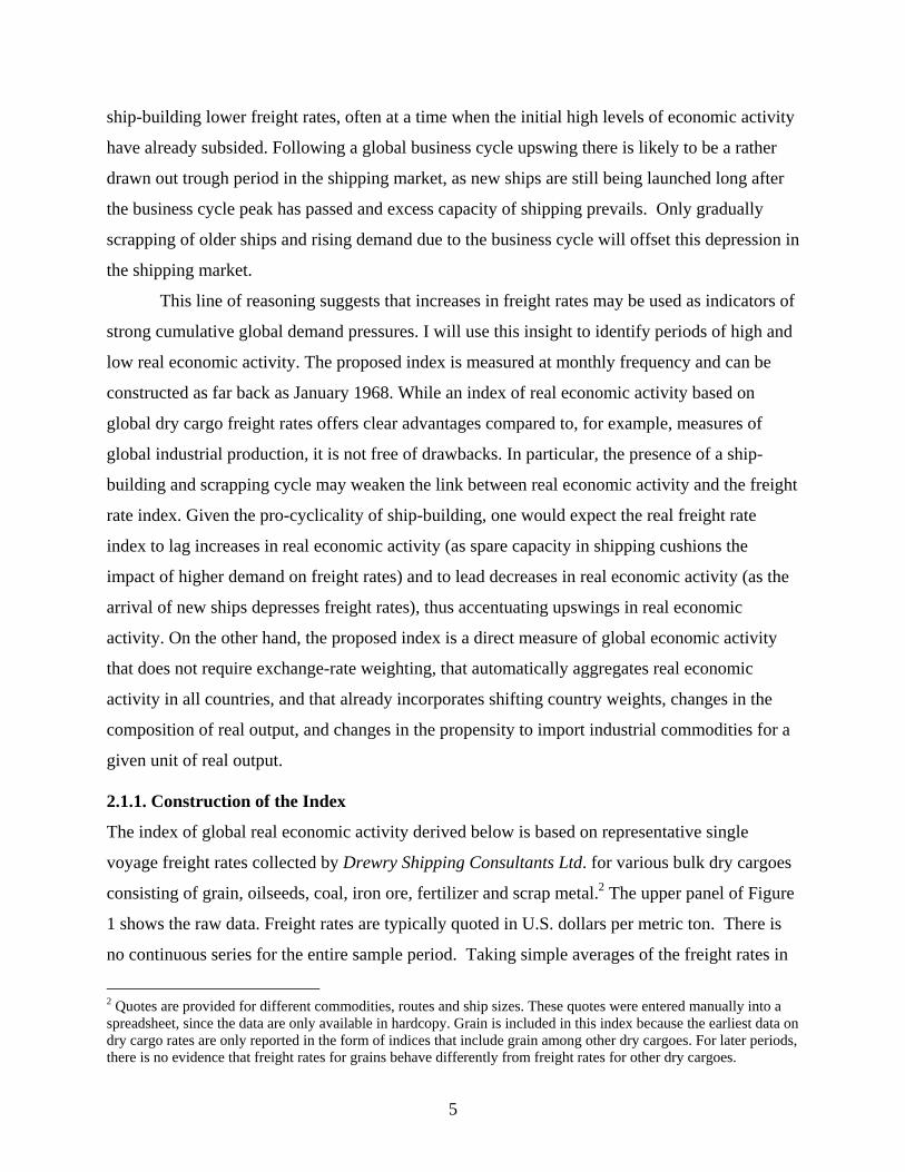
2.1.1. Construction of the Index

The index of global real economic activity derived below is based on representative single

voyage freight rates collected by Drewry Shipping Consultants Ltd. for various bulk dry cargoes

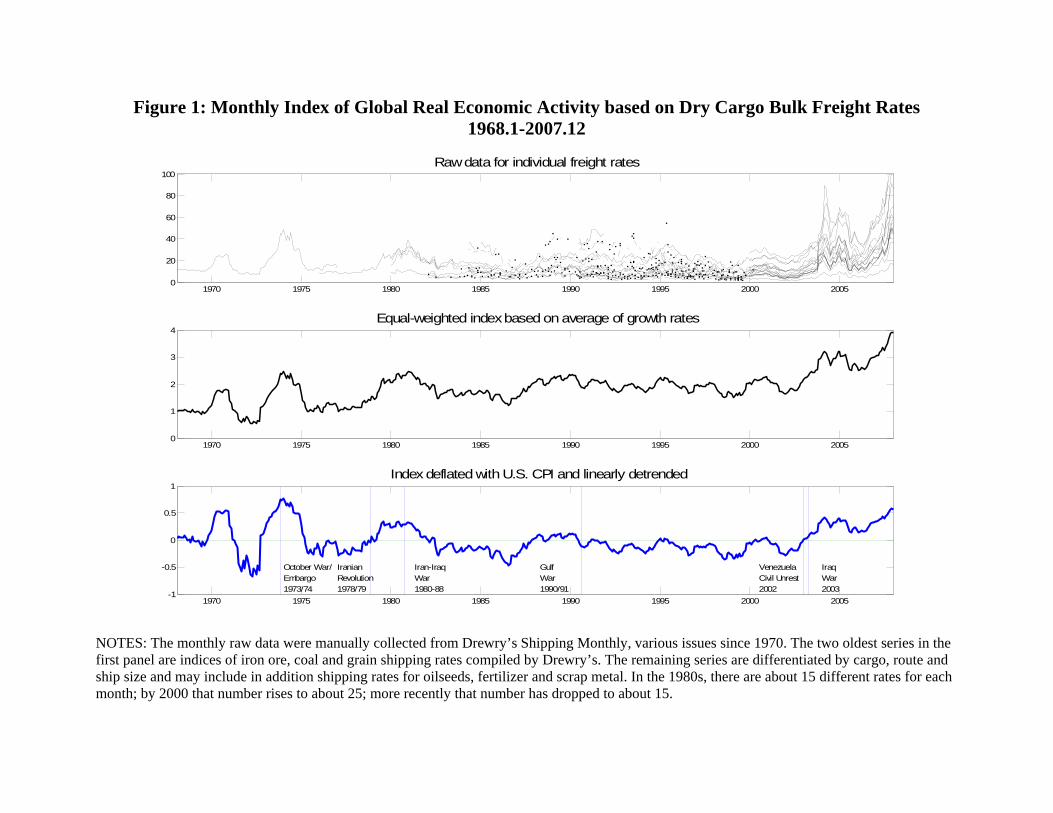
consisting of grain, oilseeds, coal, iron ore, fertilizer and scrap metal.2 The upper panel of Figure

1 shows the raw data. Freight rates are typically quoted in U.S. dollars per metric ton. There is

no continuous series for the entire sample period. Taking simple averages of the freight rates in

2 Quotes are provided for different commodities, routes and ship sizes. These quotes were entered manually into a spreadsheet, since the data are only available in hardcopy. Grain is included in this index because the earliest data on dry cargo rates are only reported in the form of indices that include grain among other dry cargoes. For later periods, there is no evidence that freight rates for grains behave differently from freight rates for other dry cargoes.

6

the upper panel would ignore the existence of fixed effects for different routes, commodities and

ship sizes. In constructing an index of dry bulk cargo freight rates I eliminate these fixed effects

as follows: I first compute the period-to-period growth rates for each series in the first panel of

Figure 1, as far as the data are available. I then take the equal-weighted average of these growth

rates, and cumulate the average growth rate, having normalized January of 1968 to unity. The

resulting index is shown in the second panel of Figure 1.3 The next step is to deflate this series

with the U.S. CPI. Finally, the real index must be detrended. As is well known, the cost of

shipping dry cargo has fallen dramatically in real terms over the decades. That trend reflects

technological advances in ship-building. It may also be related to long-run trends in the demand

for sea transport. As my interest in this paper centers on cyclical variation in ocean freight rates

rather than on long-term trends, I linearly detrend the real freight rate index. The deviations of

the real freight rates from their long-run trend are shown in the last panel of Figure 1. The linear

regression analysis in section 3 is based on the assumption that the level of global real economic

activity as it relates to industrial commodity markets is proportionate to this index.

An obvious concern is that that dry cargo freight rates may increase during oil price

shocks not because both are driven by higher demand for commodities, but because the provision

of shipping services uses bunker fuel oil as an input. In the econometric analysis below I

therefore allow for feedback from crude oil prices to shipping freight rates. The only restriction I

impose is that innovations to the shipping rates (and hence to the real activity index) will not

respond to changes in the price of crude oil within the same month. This assumption is fully

consistent with the fact that the contemporaneous correlation between shipping rates and bunker

fuel prices is essentially zero. Moreover, records in the Oil and Gas Journal indicate that during

1970-1973 the real price of bunker fuel changed very little, yet the index of real economic

activity underwent major fluctuations not unlike those in later periods.

2.1.2. The Global Business Cycle in Industrial Commodity Markets

There is little direct evidence on how the global business cycle affects industrial commodity

markets, but some anecdotal evidence. Many researchers have noted that the 1972-74 period was

characterized by a global boom, as was to a lesser extent the 1978-80 period (see, e.g.,

3 Ideally, one would like to apply different weights for different growth rates, but such weights are not provided by Drewry’s Shipping Consultants. For the same reason, equal weights are routinely used in the construction of commodity price indices.

7

Darmstadter and Landsberg 1976). We also know that the mid-1970s and the early 1980s were

characterized by worldwide recessions. Finally, we know that there has been a global boom in

commodity markets since the early 2000s driven by strong economic growth worldwide, but

particularly in Asia. Figure 1 is fully consistent with the anecdotal evidence on the relative

importance and timing of these fluctuations in global real economic activity. The two periods of

highest real activity are between late 1970 and early 1971 and between late 1972 and early 1975

with additional periods of sustained high real activity between late 1978 and late 1981 and after

late 2002. There also is a much smaller sustained expansion between early 1988 and early 1990.

The sustained high levels of real activity since 2002 are very much reminiscent of those observed

after 1979, but have been more persistent. The vertical lines in the last panel of Figure 1

correspond to major political events in oil markets. Many of these events coincided with periods

of high real economic activity and hence strong demand for industrial commodities. Thus, one

would want to be careful about associating the concurrent increases in the real price of oil with

these events. This evidence underscores the importance of disentangling the effects of demand

shocks and supply shocks on the real price of oil.

3. Decomposing the Real Price of Oil

Numerous empirical and theoretical studies have investigated the response of macroeconomic

aggregates to changes in the price of oil. Implicit in this literature is the thought experiment that

one can change the price of oil, while holding everything else constant, as would be the case if

the price of oil were exogenous. To the extent that the price of oil is actually endogenous with

respect to the macroeconomic aggregates of interest, this thought experiment is violated. If there

is no well defined cause, it becomes impossible to estimate its effect. This general principle has

been recognized dating back to the Cowles Commission. As Cooley and LeRoy (1985, p. 295)

summarize, it is inadmissible to inquire about the effect of a change in one endogenous variable

on another, when the underlying experiment that led to the assumed variation in the endogenous

variable is ambiguous.

This problem has not completely escaped attention. Implicitly or explicitly, many

researchers have assumed that at least the major increases in the price of oil can be treated as

exogenous. Recent research has demonstrated that this interpretation, which seemed reasonable

at the time, does not hold up to scrutiny (see, e.g., Kilian 2008a). This means that without

knowing what drove up the price of oil in the first place, it will be impossible to predict

8

accurately the implications of higher oil prices. In this section, I present a methodology for

decomposing unpredictable changes in the real price of oil into mutually orthogonal components

with structural economic interpretation. This decomposition has immediate implications for how

macroeconomists and policymakers should think about oil price fluctuations.

3.1. The Structural VAR Model

Consider a VAR model based on monthly data for ( ), , ,t t t tz prod rea rpo ′= Δ where tprodΔ is

the percent change in global crude oil production, trea denotes the index of real economic

activity constructed in section 2, and trpo defers to the real price of oil. The trea and trpo series

are expressed in logs. The sample period is 1973.1-2006.10.4 The structural VAR representation

is

(1) 24

01

t i t i ti

A z A zα ε−=

= + +∑ ,

where tε denotes the vector of serially and mutually uncorrelated structural innovations. I

postulate that 10A− has a recursive structure such that the reduced form errors te can be

decomposed according to 10t te A ε−= .

supply11

21 22

31 32 33

0 00

prod oil shockt t

rea aggregate demand shockt t t

rpo oil specific demand shockt t

e ae e a a

e a a a

εεε

Δ

−

⎛ ⎞ ⎛ ⎞⎡ ⎤⎜ ⎟ ⎜ ⎟⎢ ⎥≡ =⎜ ⎟ ⎜ ⎟⎢ ⎥⎜ ⎟ ⎜ ⎟⎢ ⎥⎣ ⎦⎝ ⎠ ⎝ ⎠

This model postulates a vertical short-run supply curve of crude oil. Shifts of the demand curve

driven by either of the two oil demand shocks result in an instantaneous change in the real price

of oil, as do unanticipated oil supply shocks that shift the vertical supply curve. The restrictions

on 10A− may be motivated as follows: Crude oil supply shocks (referred to as oil supply shocks

4 The starting date is dictated by the availability of the oil production data from the U.S. Department of Energy. I compute the log differences of world crude oil production in millions of barrels pumped per day (averaged by month). The real oil price series is obtained based on the refiner acquisition cost of imported crude oil, as provided by the U.S. Department of Energy since 1974.1 and extended backward as in Barsky and Kilian (2002). The nominal oil price has been deflated by the U.S. CPI.

9

for short) are defined as unpredictable innovations to global oil production.5 Crude oil supply is

assumed not to respond to innovations to the demand for oil within the same month. That

exclusion restriction is plausible because, in practice, oil-producing countries will be slow to

respond to demand shocks, given the costs of adjusting oil production and the uncertainty about

the state of the crude oil market.6

Innovations to global real economic activity that cannot be explained based on crude oil

supply shocks will be referred to as shocks to the global demand for industrial commodities (or

aggregate demand shocks for short).7 The model imposes the exclusion restriction that increases

in the real price of oil driven by shocks that are specific to the oil market will not lower global

real economic activity immediately, but with a delay of at least a month. This restriction is

consistent with the sluggish behavior of global real economic activity after each of the major oil

price increases in the sample.

Finally, innovations to the real price of oil that cannot be explained based on oil supply

shocks or aggregate demand shocks by construction will reflect changes in the demand for oil as

opposed to changes in the demand for all industrial commodities (referred to as oil-specific

demand shocks for short). The latter structural shock will reflect in particular fluctuations in

precautionary demand for oil driven by uncertainty about the availability of future oil supplies.

Whereas it potentially could also reflect other oil-market specific demand shocks, as documented

below, there are strong reasons to believe that this shock effectively represents exogenous shifts

in precautionary demand.

First, there are no other plausible candidates for exogenous oil-market specific demand

shocks. For example, while it may seem plausible that the surge in the real price of oil since 2003

was driven by an increased preference of Asian consumers for energy-using durables such as

5 In an earlier version of this paper, I further decomposed changes in the production of crude oil into crude oil supply shocks driven by exogenous political events in the Middle East, building on recent work in Kilian (2008a,b), and other crude oil supply shocks. This distinction does not change the main results of this paper. 6 If changing oil production is costly, oil producers set production based on expected trend growth in demand, and do not revise the production level in response to high-frequency variation in demand. Changes in the trend growth of demand are difficult to detect at high frequency. It takes a long time span of data to detect such a change, which suggests that production plans will be changed only infrequently. This view is consistent with evidence from interviews of Saudi officials in the early 1980s (see Yergin 1992). It is also consistent with the fact that the state-owned Saudi oil company produces forecasts of oil demand only once a year. 7 The term aggregate demand in this context does not refer to the demand for all goods and services, as in introductory macroeconomic models, but rather to the demand for all industrial commodities. I abstract from idiosyncratic shocks to the demand or supply of dry cargoes. These shocks are presumed to average out in the construction of the index of real economic activity.

10

automobiles, as I will show below, the observed increase in the real price of oil is not associated

with an increase in oil-specific demand, allowing us to rule out that interpretation. Likewise,

there is no evidence that the observed oil-specific demand shocks are associated with

unexpectedly cold winters or other weather shocks. Indeed, one would expect such shocks to

average out on a global scale. Second, the large impact effect of oil-market specific shocks

documented in section 3.2 is difficult to reconcile with shocks not driven by expectation shifts.

Third, the timing of these shocks and the direction of their effects is consistent with the timing of

exogenous events such as the outbreak of the Persian Gulf War that would be expected to affect

uncertainty about future oil supply shortfalls on a priori grounds. Fourth, the overshooting of the

price of oil in response to oil-market specific demand shocks documented in section 3.2

coincides with the predictions of theoretical models of precautionary demand shocks driven by

increased uncertainty about future oil supply shortfalls (see Alquist and Kilian 2007). Finally, the

movements in the real price of oil induced by this shock are highly correlated with independent

measures of the precautionary demand component of the real price of oil based on futures prices.

Using oil futures market data since 1989, Alquist and Kilian (2007) show that this correlation

may be as high as 80% notwithstanding the use of a completely different data set and

methodology.

Despite its simplicity, the identification scheme used in this paper allows for the

possibility that the high real price of oil in recent years as well as in the 1970s was driven in part

by unusually low U.S. interest rates reflecting the low opportunity cost of holding oil inventories

as well the weakening dollar (also see Barsky and Kilian 2002). Since lower interest rates all else

equal tend to stimulate global demand for all industrial commodities, such demand will be

reflected in the measure of aggregate demand for industrial commodities by construction. The

identification scheme also allows for the possibility that OPEC may have acted as a cartel during

part of the estimation sample. OPEC has historically tended to restrict supply in order to prop up

the price of oil. Such reductions in the supply of oil will be captured by the oil supply shock in

the model. In any event, there is little evidence that cartel activities mattered for the sample

period in question, making this point largely moot (see, e.g., Skeet 1988, Almoguera and Herrera

2007).

3.2. Empirical Results

The reduced form VAR model is consistently estimated by the least-squares method. The

11

resulting estimates are used to construct the structural VAR representation of the model.

Inference is based on a recursive-design wild bootstrap with 2,000 replications (see Gonçalves

and Kilian 2004).

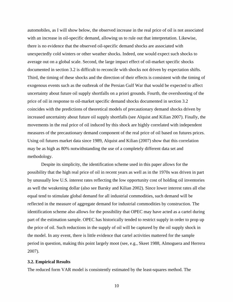
3.2.1. Quantifying the Evolution of the Oil-Demand and Oil-Supply Shocks

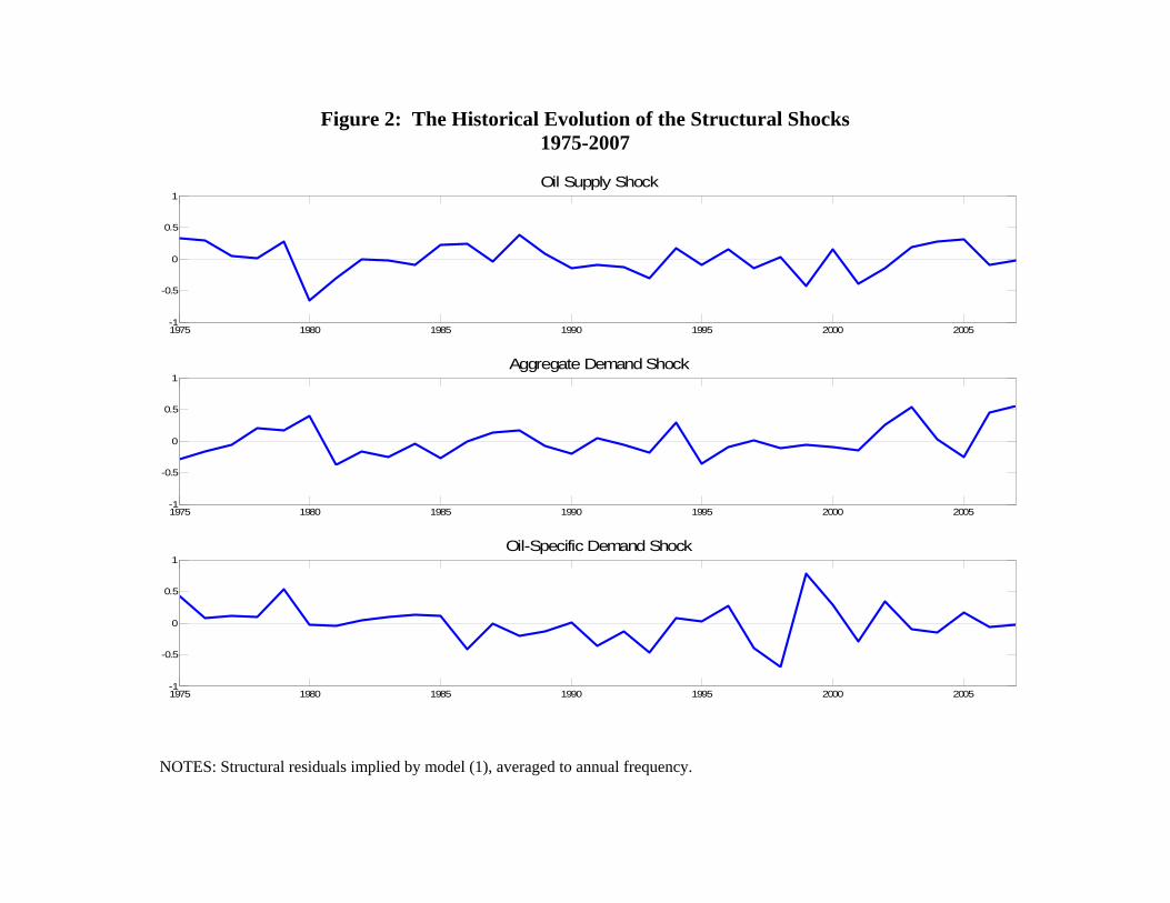
Figure 2 plots the time path of the structural shocks implied by the model (expressed as annual

averages to improve the readability of the plot). Figure 2 shows that at any point in time, the real

price of oil responds to a multitude of shocks, the composition of which evolves over time. A

case in point is the oil price shock of 1979/80. There is no evidence of a global oil supply

disruption in 1978 or 1979 (despite the cutbacks associated with the Iranian revolution which

were more than offset by increased oil production elsewhere), but there was a disruption in 1980

associated with the outbreak of the Iran-Iraq War. The years 1978, 1979, and 1980 were

characterized by repeated large positive shocks to global aggregate demand. There also was a

large unanticipated increase in oil-specific demand in 1979 (but not in 1978 or 1980), consistent

with the fact that the Iranian Revolution, the Iranian hostage crisis and the Soviet invasion of

Afghanistan all raised concerns about the future availability of oil supplies from the Middle East

in 1979. This account of what happened in 1979/80 is fully consistent with the discussion of this

episode in Barsky and Kilian (2002, 2004), but, unlike that earlier line of work, we now can

assess the quantitative importance of each of these factors.

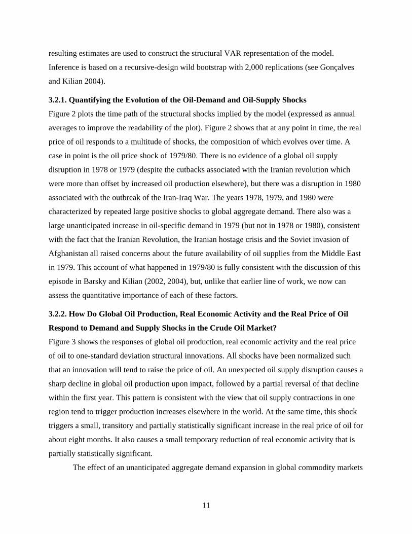
3.2.2. How Do Global Oil Production, Real Economic Activity and the Real Price of Oil

Respond to Demand and Supply Shocks in the Crude Oil Market?

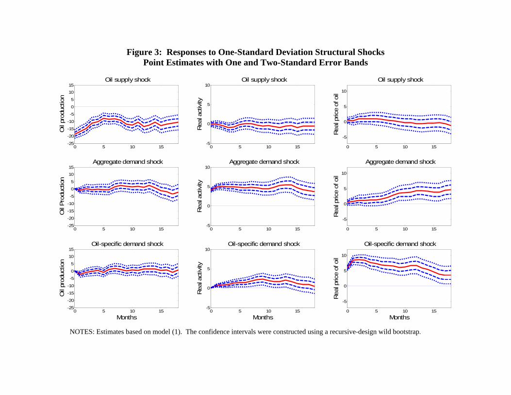
Figure 3 shows the responses of global oil production, real economic activity and the real price

of oil to one-standard deviation structural innovations. All shocks have been normalized such

that an innovation will tend to raise the price of oil. An unexpected oil supply disruption causes a

sharp decline in global oil production upon impact, followed by a partial reversal of that decline

within the first year. This pattern is consistent with the view that oil supply contractions in one

region tend to trigger production increases elsewhere in the world. At the same time, this shock

triggers a small, transitory and partially statistically significant increase in the real price of oil for

about eight months. It also causes a small temporary reduction of real economic activity that is

partially statistically significant.

The effect of an unanticipated aggregate demand expansion in global commodity markets

12

on global real economic activity is very persistent and highly significant. It begins to decline

only after 15 months. Unanticipated aggregate demand expansions temporarily increase global

oil production with a delay of half a year. There is some indication that this increase in crude oil

production is subsequently offset by production decreases. Aggregate demand expansions also

cause a large, persistent and statistically significant increase in the real price of oil. Much of the

increase in the price of oil triggered by this shock is delayed by half a year.

Unanticipated oil-market specific demand increases have an immediate, large and

persistent positive effect on the real price of oil that is highly statistically significant. There is

clear evidence of overshooting in the response as predicted by theoretical models of

precautionary demand (see Alquist and Kilian 2007). These shocks also are associated with a

temporary increase in real economic activity and a very short-run decline in oil production. Oil-

market specific demand increases do not cause an increase in global oil production.

Perhaps the most striking result in Figure 3 is the fact that unanticipated oil supply

disruptions have only a small positive effect on the real price of oil. Part of the explanation is

that oil supply disruptions in one region countries tend to trigger endogenous expansions of

crude oil production elsewhere in the world that help offset the initial production shortfall. The

small response of the real price of oil also is consistent with related evidence that oil supply

shocks have little systematic predictive power for the changes in the real price of oil (see Kilian

2008a); yet it raises the question of what – if not crude oil supply disruptions – accounts for the

apparent large increases in the real price of oil following major exogenous political events in the

Middle East. Figure 3 suggests that the answer lies in sharp increases in precautionary demand.

As shifts in precautionary demand are ultimately driven by expectations about the availability of

future oil supplies and such expectations can change almost instantaneously in response to

exogenous political events, such shocks tend to trigger an immediate and sharp increase in the

real price of oil. This explanation will be explored further in the next subsection using historical

decompositions of the real price of oil.

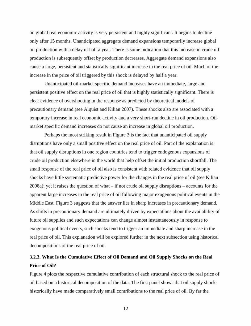
3.2.3. What Is the Cumulative Effect of Oil Demand and Oil Supply Shocks on the Real

Price of Oil?

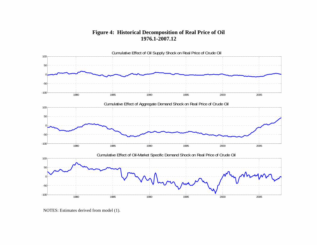
Figure 4 plots the respective cumulative contribution of each structural shock to the real price of

oil based on a historical decomposition of the data. The first panel shows that oil supply shocks

historically have made comparatively small contributions to the real price of oil. By far the

13

biggest contributions are due to the aggregate demand shock and the oil-market specific demand

shock. Whereas the aggregate demand shock caused long swings in the real price of oil, the oil-

market specific demand shock is responsible for fairly sharply defined increases and decreases in

the price of oil. This fact is consistent with the view that precautionary demand shocks may

reflect rapid shifts in the market’s assessment of the uncertainty about future oil supply

shortfalls.

It is instructive to focus on specific episodes. For example, the rapid rise in the real price

of oil in late 1979 and 1980 after the Iranian Revolution appears to be driven mainly by the

superimposition of a sharp increase in precautionary demand in 1979 on a slower-moving strong

increase in real economic activity that started two years earlier. While the cumulative effect of

oil-market specific demand peaked prior to the outbreak of the Iran-Iraq war and slowly subsided

in the early 1980s, real economic activity continued to sustain the real price of oil well into the

early 1980s. Throughout this period, oil supply shocks only served to amplify some of the short-

run dynamics of the real price of oil, sometimes raising the price of oil and lowering it at other

times. The increased importance of oil-market specific demand shocks starting in 1979 is

consistent with an increase in precautionary demand. 1979 not only was the year of Khomeini’s

arrival in Iran, but of the Iranian hostage crisis and of the Soviet invasion of Afghanistan, all of

which raised persistent fears of a regional war and the destruction of oil fields in Iran and Saudi

Arabia.

The sharp fall in the real price of oil following the collapse of the OPEC cartel in late

1985 appears to be due more to a decline in oil-market specific demand than the direct effect of

the increase in Saudi oil production in the first panel or the fall in real economic activity in the

second panel. The initial perception that the breakdown of OPEC was irreversible is likely to

have sharply lowered precautionary demand at this point. This sharp drop was partially reversed

in 1987, amid attempts by OPEC to reunite. Similarly, the sharp spike in the real price of oil in

1990/91 after the invasion of Kuwait is almost entirely due to an increase in precautionary

demand.8 Oil supply disruptions had some effect on the real price of oil in the early 1990s, but

that effect was small. The disproportionate reduction in oil-market specific demand following the

Asian crisis of 1997/98, when the real price of oil fell to an all-time low, suggests that at this

8 Kilian (2008a) arrives at the same conclusion using a different methodology.

14

point precautionary demand all but vanished.9 This effect was gradually reversed after oil prices

recovered starting in 1999. There also is clear evidence of a fall in precautionary demand

associated with 9/11. Most interestingly, the sharp rise in the real price of oil after 2000 is not

driven by global aggregate demand or by the efforts of OPEC to coordinate production, but again

by factors specific to the demand for crude oil. The most striking observation in Figure 4 is that

the rise in the real price of oil since early 2002 is almost entirely due to a surge in real economic

activity that started around 2001. There is no evidence that this price increase is driven either by

precautionary demand or by oil supply shocks.

The evidence in Figure 4 shows that not all oil price shocks are alike. There are important

differences in the relative contribution of the three structural shocks to the real price of oil

between the Iran-Iraq War and the Iranian Revolution, for example, or between the Persian Gulf

War and the period following the Iraq War and the civil unrest in Venezuela. Nevertheless, there

are some regularities in that all major oil price increases appear driven primarily by demand

shocks in the oil market. This is true even during episodes commonly associated with oil supply

shocks in the Middle East. My results paint a very different picture of how exogenous political

events in the Middle East affect the real price of oil than postulated in the existing literature. The

traditional approach has been to quantify exogenous variation in actual crude oil production in

OPEC countries and to relate this variation to changes in the price of crude oil (see, e.g.,

Hamilton 2003; Kilian 2008a). That approach fails to capture shifts in market expectations that

are not reflected in observed changes to crude oil production. Not surprisingly, as has been

documented in Barsky and Kilian (2002, 2004) and Kilian (2008a), production-based accounts of

oil price shocks do not match up well with the timing of oil price changes and with historical

accounts of the crude oil market during oil crises such as the Iranian Revolution. The results of

this section, in contrast, suggest that the most important channel by which exogenous events such

as wars or revolutions affect the real price of oil is through their effect on precautionary demand

for oil. The latter channel can produce immediate and potentially large effects on the real price of

oil through shifts in the uncertainty about future oil supply shortfalls, even when crude oil

production has not changed. This point has been recognized for a long time, but it has never been

quantified before, the fundamental difficulty being that expectations shifts related to uncertainty

9 It can be shown that this drop in oil-market specific demand pre-dates the sharp drop in oil inventories in 1999/2000 and hence is unlikely to be driven by inventory adjustments. Rather inventory policies seem to have changed in response to falling oil prices.

15

about future oil supply shortfalls are not observable and not linearly related to observables.

3.2.4. Sensitivity analysis

The approach to identifying structural shocks to the real price of oil adopted in this paper heavily

relies on delay restrictions that are economically plausible only at the monthly frequency.

Measuring shifts in the demand for industrial commodities driven by global real economic

activity is a challenge, especially at monthly frequency. An alternative measure of monthly

global real economic activity would be world industrial production. Even for indices of industrial

production, however, the problems of exchange rate weighting remain and technological changes

over time may affect the link from rising production to the global demand for industrial

commodities. Moreover, suitable monthly data on world industrial production do not exist. The

closest available proxy is an index of OECD industrial production that excludes emerging

economies in Asia such as China and India, whose demand for industrial raw materials is thought

to be fueling the surge in industrial commodity and oil prices especially since 2002. Linearly

detrended OECD industrial production exhibits the same patterns during the 1970s and early

1980s, as the index based on shipping rates, but fails to capture the boom since 2002. Using this

index as a measure of real activity in the VAR model of section 3 results in very similar

estimates of the responses to oil supply shocks and to oil-specific demand shocks. It also

produces a statistically significant and positive response to aggregate demand shocks, but,

predictably, that response is smaller than in the baseline model. The model by construction

attributes much of the recent build-up in oil prices to the precautionary demand shock rather than

the aggregate demand shock, because OECD industrial production data do not reflect the growth

of industrial production in Asia at the end of the sample. This sensitivity analysis highlights the

importance of using a truly global measure of real activity.

4. Understanding the Effects of Oil Price Disturbances on the U.S. Economy

4.1. Regression Model

A question of considerable interest is how the structural innovations in model (1) relate to U.S.

macroeconomic aggregates such as CPI inflation or real GDP growth. The main problem in

answering this question is that the latter aggregate is not available at monthly frequency.10 While

10 I do not use interpolated real GDP growth data. One reason is that interpolation is known to cause spurious dynamics in general. In this case, in particular, there also is a second reason not to use interpolation. Standard interpolation methods use monthly data on industrial production to infer movements in real GDP within the quarter.

16

one could construct an analogous structural VAR model (1) on data aggregated to quarterly

frequency, at that frequency the identifying assumptions would no longer be credible. Instead I

construct measures of the quarterly shocks by averaging the monthly structural innovations for

each quarter: 3

, ,1

1ˆ ˆ , 1,2,33jt j t i

i

jζ ε=

= =∑ ,

where , ,ˆ j t iε refers to the estimated residual for the jth structural shock in the ith month of the tth

quarter of the sample.11 Under the identifying assumption that within a given quarter there is no

feedback from tyΔ and tπ to ˆjtζ , 1,2,3,j = these shocks can be treated as predetermined and we

can examine their effects on U.S. macroeconomic aggregates based on the regressions:

(2) 12

0

ˆ , 1,2,3t j ji jt i jti

y u jα φ ζ −=

Δ = + + =∑

and

(3) 12

0

ˆ , 1,2,3t j ji jt i jti

v jπ δ ψ ζ −=

= + + =∑

where jtu and jtv are potentially serially correlated errors. In this regression model the impulse

response coefficients at horizon h correspond to jhφ and jhψ , respectively. Thus, the number of

lags is determined by the maximum horizon of the impulse response function, which is set to 12

quarters. In conducting inference on the response estimates implied by models (2) and (3), the

presence of serial correlation in the error term is dealt with by using block bootstrap methods.12

The assumption that ˆ ,jtζ 1,2,3,j = is predetermined with respect to U.S. real GDP growth is

not testable, but may be defended as follows: First, consider 1̂ .tζ To the extent that an

unanticipated reduction (expansion) in crude oil supply would be associated with a decline

(increase) in real GDP growth within the quarter, the correlation of the innovations should be

Since industrial production is a measure of gross output that may behave very differently from real GDP (a measure of value added) in response to oil shocks, as discussed in Barsky and Kilian (2002), the concern is that interpolated “monthly” real GDP data will behave like industrial production, thus invalidating the analysis. 11 Although these quarterly averages will not be exactly uncorrelated, their empirical correlation is so low, that little is lost by treating them as uncorrelated. 12 All results shown below are for block size 4 and 20,000 bootstrap replications. Results based on block size 8 are very similar. It is important to note that these confidence intervals do not account for the fact that the residuals used in the regressor matrix are generated regressors. Controlling for this problem is complicated by the fact that the regression procedure involves data at both monthly and quarterly frequency.

17

positive. To the extent that an unanticipated increase in U.S. real GDP growth would tend to call

forth within the quarter an increase in global crude oil production, the correlation of real GDP

innovations with the global oil supply shock should also be positive. Since the empirical

correlation is very low, as can be verified by computing the autoregressive residuals of U.S. real

GDP growth and correlating them with 1̂ ,tζ we know that neither direction of causality matters

much at quarterly frequency, and that the global oil supply shock can be treated as predetermined

with respect to U.S. real GDP growth.

Next consider 2ˆ .tζ If the intuition were right that positive innovations to U.S. real GDP

growth stimulate global demand for industrial commodities, we would expect the correlation

between innovations to U.S. real GDP growth and global aggregate demand shocks to be

positive. To the extent that causation runs the other way from global demand shocks for

industrial commodities to innovations to U.S. real GDP growth, that correlation should also be

positive. The fact that the contemporaneous correlation of these innovations, computed as

discussed before, is essentially zero in the data implies that neither causal link is quantitatively

important at the quarterly frequency. Hence, we may treat global aggregate demand shocks as

predetermined with respect to U.S. real GDP growth.

Finally, consider 3̂ .tζ Positive innovations to U.S. real GDP growth may raise precautionary

demand; yet unanticipated increases in precautionary demand will increase the price of oil and

hence may lower U.S. real GDP growth on impact. Since it is conceivable that these two effects

may offset one another at least in part, we cannot use the low empirical correlation of these

innovations to argue that there is no feedback from U.S. real GDP innovations to the

precautionary demand shock. Nevertheless, a plausibility check helps defend the assumption that

3̂tζ is predetermined. Precautionary demand reflects uncertainty about the shortfall of future oil

supply relative to expected demand for oil at medium-term or long-term horizons. An innovation

to quarterly U.S. real GDP growth will have negligible effects on the estimate of that trend

component under any conceivable model of trend growth in demand, and hence negligible

effects on precautionary demand.

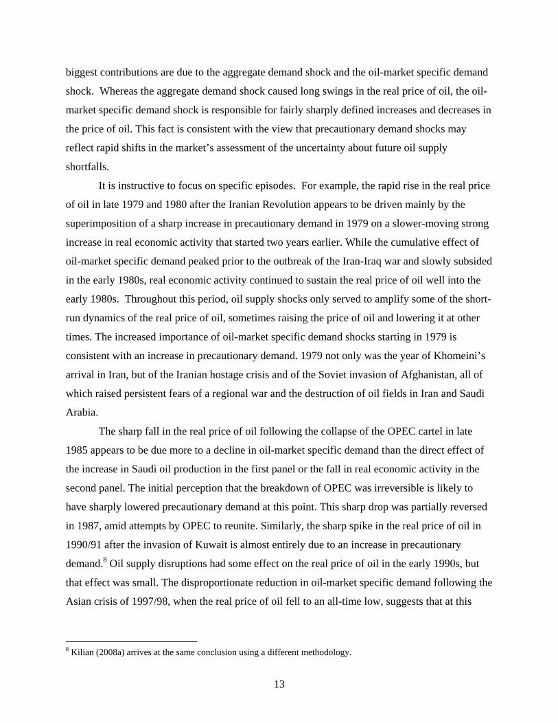
4.2. Does it Matter for U.S. Macroeconomic Performance Why the Price of Oil Increased?

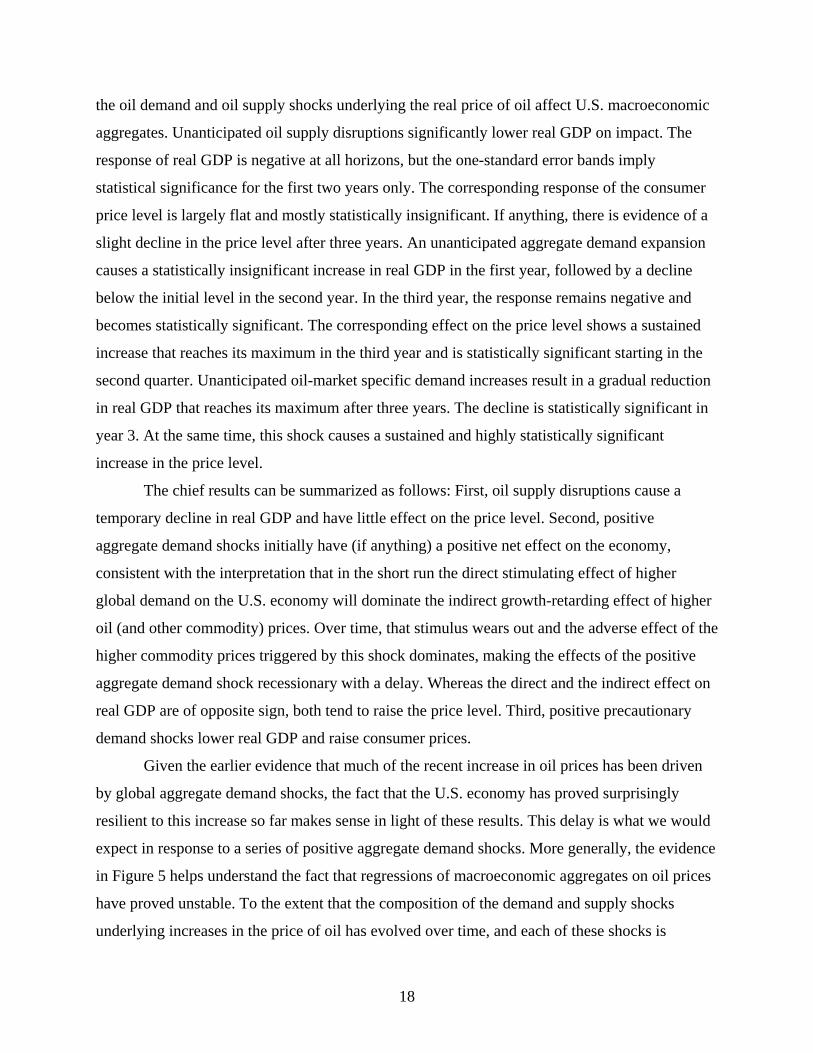
Figure 5 summarizes the responses of the level of U.S. real GDP and the level of the CPI to each

of the three shocks defined earlier. The results in Figure 5 illustrate important differences in how

18

the oil demand and oil supply shocks underlying the real price of oil affect U.S. macroeconomic

aggregates. Unanticipated oil supply disruptions significantly lower real GDP on impact. The

response of real GDP is negative at all horizons, but the one-standard error bands imply

statistical significance for the first two years only. The corresponding response of the consumer

price level is largely flat and mostly statistically insignificant. If anything, there is evidence of a

slight decline in the price level after three years. An unanticipated aggregate demand expansion

causes a statistically insignificant increase in real GDP in the first year, followed by a decline

below the initial level in the second year. In the third year, the response remains negative and

becomes statistically significant. The corresponding effect on the price level shows a sustained

increase that reaches its maximum in the third year and is statistically significant starting in the

second quarter. Unanticipated oil-market specific demand increases result in a gradual reduction

in real GDP that reaches its maximum after three years. The decline is statistically significant in

year 3. At the same time, this shock causes a sustained and highly statistically significant

increase in the price level.

The chief results can be summarized as follows: First, oil supply disruptions cause a

temporary decline in real GDP and have little effect on the price level. Second, positive

aggregate demand shocks initially have (if anything) a positive net effect on the economy,

consistent with the interpretation that in the short run the direct stimulating effect of higher

global demand on the U.S. economy will dominate the indirect growth-retarding effect of higher

oil (and other commodity) prices. Over time, that stimulus wears out and the adverse effect of the

higher commodity prices triggered by this shock dominates, making the effects of the positive

aggregate demand shock recessionary with a delay. Whereas the direct and the indirect effect on

real GDP are of opposite sign, both tend to raise the price level. Third, positive precautionary

demand shocks lower real GDP and raise consumer prices.

Given the earlier evidence that much of the recent increase in oil prices has been driven

by global aggregate demand shocks, the fact that the U.S. economy has proved surprisingly

resilient to this increase so far makes sense in light of these results. This delay is what we would

expect in response to a series of positive aggregate demand shocks. More generally, the evidence

in Figure 5 helps understand the fact that regressions of macroeconomic aggregates on oil prices

have proved unstable. To the extent that the composition of the demand and supply shocks

underlying increases in the price of oil has evolved over time, and each of these shocks is

19

associated with a distinct response pattern, this outcome is exactly what we would expect.

5. Conclusion

A recurring question in theoretical, empirical and policy work is what the effects of higher oil

prices are on U.S. macroeconomic aggregates. The main point of the paper has been that the

traditional thought experiment that this literature appeals to in answering this question is not well

defined because it implicitly presumes that one can hold everything else fixed, while varying the

price of oil. There are two reasons why this ceteris paribus assumption is inappropriate. One is

the existence of reverse causality from macroeconomic aggregates to oil prices (see, e.g., Barsky

and Kilian 2002). The second reason is that oil prices are driven by structural demand and supply

shocks which may have direct effects on the U.S. economy as well as indirect effects operating

through the price of oil. For example, an innovation to the global business cycle (that is

orthogonal to innovations to the U.S. economy) will stimulate the U.S. economy directly, but it

will also drive up the price of oil and other imported commodities, thereby slowing U.S.

domestic growth. Thus, by construction, we cannot think of varying the price of oil without

varying other variables.

This second point, while seemingly self-evident if we were discussing any other

commodity market, is new and has powerful implications. For example, it helps explain the

instability of regressions based on oil prices and, in particular, why higher oil prices seem to

matter less today than in the 1970s and early 1980s (this point has been discussed at length in

Kilian 2008c). It also helps us understand how strong growth and booming stock markets can

coexist with rising oil prices, and why there has not been a major recession in the U.S. yet

despite the surge in oil prices in recent years (also see Kilian and Park 2007).

More generally, my analysis implies that existing approaches to modeling oil price

shocks must be rethought. First, it suggests that macroeconomic models built on the assumption

of exogenous oil prices are potentially misleading and their usefulness for applied work is

unclear. Understanding the transmission of oil price shocks to the U.S. economy will require an

entirely new class of theoretical models that endogenizes the price of oil rather than relying on

the assumption of exogenously given oil prices. A recent example of such a model is Bodenstein,

Erceg, and Guerrieri (2007).

Second, models of endogenous oil prices should focus on the demand side of the oil

market. My analysis showed that the traditional emphasis on physical oil supply shocks in

20

explaining oil price shocks is misplaced. Instead, expectation shifts deserve a much greater role

in models of the oil price. A recent example of such a model is Alquist and Kilian (2007).

Likewise, the impact of the global business cycle on the demand for oil (including structural

shifts in the demand for oil related to the emergence of new economies) requires explicit

modeling. The work by Bodenstein et al. (2007) is a first step in this direction.

Third, my analysis sheds light on the interpretation of macroeconomic VAR models that

include the price of oil. To the extent that each of the demand and supply shocks in the crude oil

market is predetermined, the innovation to the real price of oil will also be predetermined,

because it can be written as a weighted average of these structural shocks. This fact allows one to

estimate the effect of an average oil price innovation on macroeconomic aggregates from

recursively identified vector autoregressions in which the percent change in the real price of oil

is ordered first. Under standard assumptions, the resulting response estimates will be

asymptotically valid as a measure of the expected response to this shock (see Kilian 2008c).

Nevertheless, since this expectation by construction reflects the average composition of oil

demand and oil supply shocks in the sample period, these estimates may be misleading, when it

comes to judging the macroeconomic effects of a specific oil price shock.

Fourth, empirical models of the monetary policy response to oil prices in the tradition of

Bernanke, Gertler and Watson (1997) may provide an approximation to the actual policy

behavior of the Federal Reserve during certain historical episodes, but they are fundamentally

misspecified in that they postulate the same response to oil price innovations regardless of the

composition of that shock. There is no compelling economic reason for the Federal Reserve to

respond to oil price innovations in general, once the price of oil is treated as endogenous. Rather

the Fed must focus on the underlying determinants of the price of oil. This point has recently

been illustrated in the context of a specific example by Nakov and Pescatori (2007).

References

Almoguera, P.A., and A.M. Herrera (2007), “Testing for the Cartel in OPEC: Noncooperative Collusion or just Noncooperative?” mimeo, Department of Economics, Michigan State University. Alquist, R., and L. Kilian (2007), “What Do We Learn from the Price of Crude Oil Futures?” mimeo, Department of Economics, University of Michigan.

21

Barsky, R.B., and L. Kilian (2002), “Do We Really Know that Oil Caused the Great Stagflation? A Monetary Alternative,” in: NBER Macroeconomics Annual 2001, B.S. Bernanke and K. Rogoff (eds.), MIT Press: Cambridge, MA, 137-183. Barsky, R.B., and L. Kilian (2004), “Oil and the Macroeconomy Since the 1970s,” Journal of Economic Perspectives, 18(4), 115-134. Bernanke, B.S., M. Gertler, and M. Watson (1997), “Systematic Monetary Policy and the Effects of Oil Price Shocks,” Brookings Papers on Economic Activity, 1, 91-142. Bodenstein, M., C.J. Erceg, and L. Guerrieri (2007), “Oil Shocks and External Adjustment,”

mimeo, Federal Reserve Board.

Cooley, T.F., and S. LeRoy (1985), “Atheoretical Macroeconometrics: A Critique,”, Journal of Monetary Economics, 16, 283-308. Darmstadter, J., and H.H. Landsberg (1976), “The Economic Background,” in R. Vernon (ed.), The Oil Crisis, Norton: New York. Drewry Shipping Consultants Ltd, Shipping Statistics and Economics, monthly, various issues since 1970. Gonçalves, S., and L. Kilian (2004), “Bootstrapping Autoregressions with Conditional Heteroskedasticity of Unknown Form,” Journal of Econometrics, 123, 89-120. Hamilton, J.D. (2003), “What is an Oil Shock?” Journal of Econometrics, 113, 363-398. Isserlis, L. (1938), “Tramp Shipping Cargoes and Freights,” Journal of the Royal Statistical Society, 101, 53-134. Kilian, L. (2008a), “Exogenous Oil Supply Shocks: How Big Are They and How Much Do They Matter for the U.S. Economy?” Review of Economics and Statistics, 90, 216- 240. Kilian, L. (2008b), “A Comparison of the Effects of Exogenous Oil Supply Shocks on Output and Inflation in the G7 Countries,” Journal of the European Economic Association, 6, 78-121. Kilian, L. (2008c), “The Economic Effects of Energy Price Shocks,” in preparation for the Journal of Economic Literature. Kilian, L., and C. Park (2007), “The Impact of Oil Price Shocks on the U.S. Stock Market,” CEPR Discussion Paper No. 6166, March 2007.

22

Klovland, J.T. (2004), “Business Cycles, Commodity Prices and Shipping Freight Rates: Some Evidence from the pre-WWI Period,” paper presented at the Workshop on Market Performance and the Welfare Gains of Market Integration in History, European University Institute, Florence, Italy, July 1-4, 2004. Nakov, A., and A. Pescatori (2007), “Inflation-Output Gap Trade-off with a Dominant Oil

Supplier,” mimeo, Federal Reserve Bank of Cleveland. Oil and Gas Journal, various issues since 1970. Skeet, I. (1988), OPEC: Twenty-Five Years of Prices and Politics, Cambridge University Press: Cambridge, UK. Stopford, M. (1997), Maritime Economics. 2nd ed., Routledge: London, U.K. Tinbergen, J. (1959), “Tonnage and Freight,” in Jan Tinbergen Selected Papers, North Holland: Amsterdam, 93-111. Yergin, D. (1992), The Prize. The Epic Quest for Oil, Money, and Power. Simon and Schuster: New York.

1970 1975 1980 1985 1990 1995 2000 20050

20

40

60

80

100Raw data for individual freight rates

1970 1975 1980 1985 1990 1995 2000 20050

1

2

3

4Equal-weighted index based on average of growth rates

1970 1975 1980 1985 1990 1995 2000 2005-1

-0.5

0

0.5

1

October War/Embargo1973/74

IranianRevolution1978/79

Iran-IraqWar1980-88

GulfWar1990/91

VenezuelaCivil Unrest2002

IraqWar2003

Index deflated with U.S. CPI and linearly detrended

Figure 1: Monthly Index of Global Real Economic Activity based on Dry Cargo Bulk Freight Rates 1968.1-2007.12

NOTES: The monthly raw data were manually collected from Drewry’s Shipping Monthly, various issues since 1970. The two oldest series in the first panel are indices of iron ore, coal and grain shipping rates compiled by Drewry’s. The remaining series are differentiated by cargo, route and ship size and may include in addition shipping rates for oilseeds, fertilizer and scrap metal. In the 1980s, there are about 15 different rates for each month; by 2000 that number rises to about 25; more recently that number has dropped to about 15.

1975 1980 1985 1990 1995 2000 2005-1

-0.5

0

0.5

1Oil Supply Shock

1975 1980 1985 1990 1995 2000 2005-1

-0.5

0

0.5

1Aggregate Demand Shock

1975 1980 1985 1990 1995 2000 2005-1

-0.5

0

0.5

1Oil-Specific Demand Shock

Figure 2: The Historical Evolution of the Structural Shocks 1975-2007

NOTES: Structural residuals implied by model (1), averaged to annual frequency.

0 5 10 15-25

-20

-15

-10

-5

0

5

10

15Oil supply shock

Oil

prod

uctio

n

0 5 10 15-5

0

5

10Oil supply shock

Rea

l act

ivity

0 5 10 15

-5

0

5

10

Oil supply shock

Rea

l pric

e of

oil

0 5 10 15-25

-20

-15

-10

-5

0

5

10

15Aggregate demand shock

Oil

Prod

uctio

n

0 5 10 15-5

0

5

10Aggregate demand shock

Rea

l act

ivity

0 5 10 15

-5

0

5

10

Aggregate demand shock

Rea

l pric

e of

oil

0 5 10 15-25

-20

-15

-10

-5

0

5

10

15Oil-specific demand shock

Oil

prod

uctio

n

Months0 5 10 15

-5

0

5

10Oil-specific demand shock

Rea

l act

ivity

Months0 5 10 15

-5

0

5

10

Oil-specific demand shock

Rea

l pric

e of

oil

Months

Figure 3: Responses to One-Standard Deviation Structural Shocks Point Estimates with One and Two-Standard Error Bands

NOTES: Estimates based on model (1). The confidence intervals were constructed using a recursive-design wild bootstrap.

1980 1985 1990 1995 2000 2005-100

-50

0

50

100Cumulative Effect of Oil Supply Shock on Real Price of Crude Oil

1980 1985 1990 1995 2000 2005-100

-50

0

50

100Cumulative Effect of Aggregate Demand Shock on Real Price of Crude Oil

1980 1985 1990 1995 2000 2005-100

-50

0

50

100Cumulative Effect of Oil-Market Specific Demand Shock on Real Price of Crude Oil

Figure 4: Historical Decomposition of Real Price of Oil 1976.1-2007.12

NOTES: Estimates derived from model (1).

0 2 4 6 8 10 12-15

-10

-5

0

5

10

Rea

l GD

P

Crude Oil Supply Shock

0 2 4 6 8 10 12-15

-10

-5

0

5

10

Rea

l GD

P

Aggregate Demand Shock

0 2 4 6 8 10 12-15

-10

-5

0

5

10

Rea

l GD

P

Oil-Market Specific Demand Shock

Quarters

0 2 4 6 8 10 12-20

-10

0

10

20

30

CP

I

Crude Oil Supply Shock

0 2 4 6 8 10 12-20

-10

0

10

20

30

CP

I

Aggregate Demand Shock

0 2 4 6 8 10 12-20

-10

0

10

20

30

CP

I

Oil-Market Specific Demand Shock

Quarters

Figure 5: Responses of U.S. Real GDP and CPI Level to Each Structural Shock Point Estimates with One and Two-Standard Error Bands

NOTES: The plots show the cumulated responses estimated from models (2) and (3).