Embed Size (px)
Citation preview
Note Detection and Multiple Fundamental Frequency Estimation inPiano Recordings
by
Matthew Thompson
A thesis submitted to the Graduate Faculty ofAuburn University
in partial fulfillment of therequirements for the Degree of
Master of Science
Auburn, AlabamaDecember 12, 2015
Keywords: automatic music transcription, note onset detection, multiplefundamental frequency estimation
Copyright 2015 by Matthew Thompson
Approved by
Lloyd Riggs, Chair, Professor of Electrical and Computer EngineeringStanley Reeves, Professor of Electrical and Computer Engineering
Myoung An, Associate Research Professor of Computer Science and SoftwareEngineering
Abstract
Automatic music transcription (AMT) is a difficult signal processing problem,
which has, in the past decade or two, begun to receive proper treatment. An overview
of the problem with a focus on the nature of music signals is given, and two significant
AMT challenges are addressed in detail—note onset detection and multiple funda-
mental frequency estimation. Recent work on these problems is summarized, and
an algorithm considering both challenges in the context of piano audio transcription
is proposed. A portion of the algorithm concerning multiple fundamental frequency
estimation is, to the knowledge of this author, unique. The algorithm is tested, and
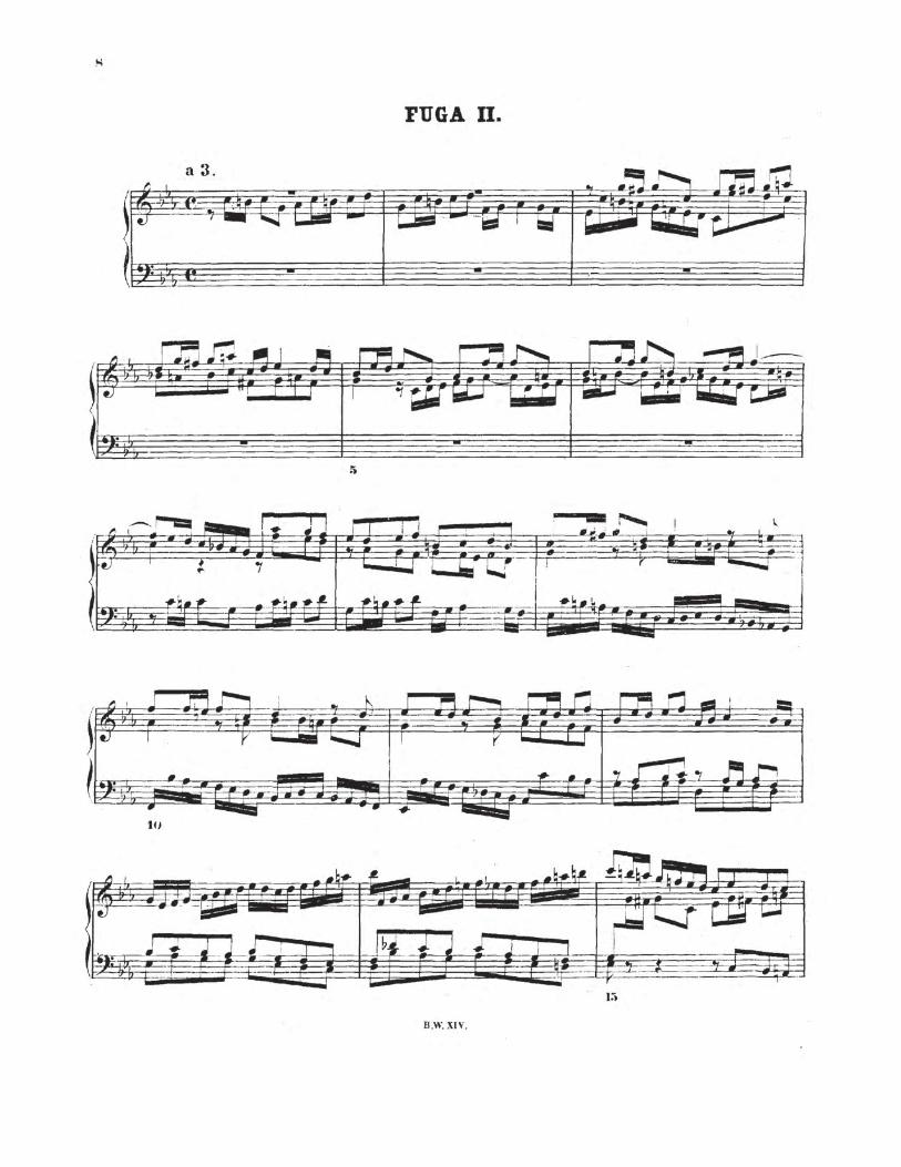
results are shown for a recording of Bach’s BWV 847 fugue.
ii
Acknowledgments
The author would like to thank Dr. Lloyd Riggs, Dr. Stanley Reeves, Dr.
Myoung An, and Dr. Shumin Wang for their support of his interest in this problem
and for their most helpful input and discussion. In particular, appreciation is due to
Dr. An for her extraordinary support and encouragement of the author’s education,
making this endeavor possible. Also, thanks is offered to each who read the draft
and provided feedback. Finally, the author would like to thank his parents, without
whose loving encouragement he would not be where he is now.
iii
Table of Contents
Abstract . . . . . . . . . . . . . . . . . . . . . . . . . . . . . . . . . . . . . . . ii
Acknowledgments . . . . . . . . . . . . . . . . . . . . . . . . . . . . . . . . . . iii
List of Figures . . . . . . . . . . . . . . . . . . . . . . . . . . . . . . . . . . . vi
List of Tables . . . . . . . . . . . . . . . . . . . . . . . . . . . . . . . . . . . . viii
1 Introduction . . . . . . . . . . . . . . . . . . . . . . . . . . . . . . . . . . 1
2 Overview of Automatic Music Transcription . . . . . . . . . . . . . . . . 4
2.1 Digital Audio Files . . . . . . . . . . . . . . . . . . . . . . . . . . . . 5
2.2 Considerations on the Nature of Musical Signals . . . . . . . . . . . . 6
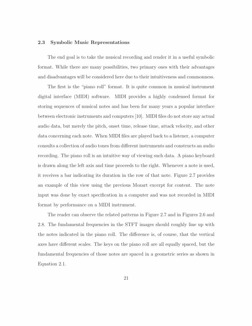
2.3 Symbolic Music Representations . . . . . . . . . . . . . . . . . . . . . 21
3 Problem Considered in This Thesis . . . . . . . . . . . . . . . . . . . . . 24
4 Note Onset Detection . . . . . . . . . . . . . . . . . . . . . . . . . . . . . 26
4.1 Review of Approaches . . . . . . . . . . . . . . . . . . . . . . . . . . 26
4.2 Suggested Approach . . . . . . . . . . . . . . . . . . . . . . . . . . . 28
5 Multiple Fundamental Frequency Estimation . . . . . . . . . . . . . . . . 30
5.1 Review of Approaches . . . . . . . . . . . . . . . . . . . . . . . . . . 30
5.2 Suggested Approach . . . . . . . . . . . . . . . . . . . . . . . . . . . 33
6 Algorithm Description and Results . . . . . . . . . . . . . . . . . . . . . 39
6.1 Note Onset Detection . . . . . . . . . . . . . . . . . . . . . . . . . . . 39
6.2 Calibration Signal . . . . . . . . . . . . . . . . . . . . . . . . . . . . . 44
iv

6.3 Multiple Fundamental Frequency Estimation . . . . . . . . . . . . . . 44
6.4 Transcription Results . . . . . . . . . . . . . . . . . . . . . . . . . . . 47
7 Conclusions and Future Work . . . . . . . . . . . . . . . . . . . . . . . . 54
Bibliography . . . . . . . . . . . . . . . . . . . . . . . . . . . . . . . . . . . . 55
Appendices . . . . . . . . . . . . . . . . . . . . . . . . . . . . . . . . . . . . . 58
A Bach BWV 847 Score . . . . . . . . . . . . . . . . . . . . . . . . . . . . . 59
v
List of Figures
2.1 Time sampling of middle C played on a piano . . . . . . . . . . . . . . . 7
2.2 Spectrum of middle C played on a piano . . . . . . . . . . . . . . . . . . 8
2.3 Spectrum of A0 played on a piano . . . . . . . . . . . . . . . . . . . . . . 15
2.4 Times series of Mozart piano sonata K.545, measures 1-4 . . . . . . . . . 17
2.5 Spectrum of Mozart piano sonata K.545, measures 1-4 . . . . . . . . . . 18
2.6 STFT of Mozart piano sonata K.545, measures 1-4, left channel . . . . . 19
2.7 Piano roll view of Mozart piano sonata K.545, measures 1-4 . . . . . . . 19
2.8 STFT of Mozart piano sonata K.545, measures 1-4, right channel . . . . 20
2.9 Sheet music view of Mozart piano sonata K.545, measures 1-4 . . . . . . 20
5.1 Test chord, power spectral summing, left channel . . . . . . . . . . . . . 36
5.2 Test chord, magnitude summing and maximum, left channel . . . . . . . 37
6.1 Onset-finding intermediate of Mozart piano sonata K.545, measures 1-4 . 41
vi
6.2 Onset detection of Mozart piano sonata K.545, measures 1-4 . . . . . . . 42
6.3 Onset detection of trill in Mozart piano sonata K.576 . . . . . . . . . . . 43
6.4 Onset detection of typical calibration signal . . . . . . . . . . . . . . . . 45
6.5 Piano roll view of Mozart piano sonata K.545, measures 1-4 . . . . . . . 49
6.6 Transcription of Mozart piano sonata K.545, measures 1-4 . . . . . . . . 49
6.7 Transcription of Mozart piano sonata K.545, measures 1-4, hard threshold 50
6.8 Piano roll view of Bach fugue BWV 847, measures 1-17 . . . . . . . . . . 51
6.9 Transcription of Bach fugue BWV 847, measures 1-17 . . . . . . . . . . . 51
6.10 Piano roll view of Bach fugue BWV 847, measures 15-31 . . . . . . . . . 52
6.11 Transcription of Bach fugue BWV 847, measures 15-31 . . . . . . . . . . 52
6.12 Transcription of Bach fugue BWV 847, measures 1-17, hard threshold . . 53
6.13 Transcription of Bach fugue BWV 847, measures 15-31, hard threshold . 53
vii
List of Tables
2.1 Piano key fundamental frequencies in equal temperament . . . . . . . . . 10
viii
Endlich soll auch der Finis oder End-Ursache aller Music
und also auch des General-Basses seyn
nichts als nur GOttes Ehre und Recreation des Gemuhts.
—Friderich Erhard Niedtens, Musicalische Handleitung
Chapter 1
Introduction
Among the myriad signals receiving the attention of the signal processing com-
munity, musical signals comprise a diverse and complex collection which is only
recently beginning to receive the focus it is due. The art of music has accompanied
human culture for thousands of years, and many authors have commented on its
mysterious power of expression. This expression has taken shape in so many styles,
with so many instruments, voices, and combinations thereof, conveying so many
emotions, that to fathom what is compassed by the single word music seems akin to
fathoming the size of a galaxy.
Many types of signals like sonar, radar, and communications signals are designed
specifically with automatic signal processing in mind. Musical signals differ and,
along with speech signals, have throughout their history been designed chiefly with
the human ear in mind. This immediately introduces potential challenges as the
brain has remarkable abilities in pattern recognition and consideration of context.
To draw distinction between speech and music, speech is first a conveyance of factual
information, notwithstanding the large volume of literary art, while music seems to
be foremost an aesthetic medium. Notable exceptions would be musical lines used
practically in the military, for instance, where a bugle might signal a muster, a
charge, or a retreat, and a drum might facilitate the organized march of a unit.
1
Science fiction enthusiasts will be quick to call attention to the five-note motif which
is instrumental in communication with the extra-terrestrials in Close Encounters of
the Third Kind. Again, though, these are the exceptions. Suppose one wishes to use a
search algorithm to find speech recordings on a particular subject. The goal, at least,
is rather straightforward; determine the spoken words and analyze the ordering of
words for meaning. An analogous search for music is not so straightforward. Indeed,
we would resolve notes and rhythms in a recording, but then how would one search
a musical database for mournful, or frightening, or joyous music? This is a more
complex task. Perhaps because of demand and because of the comparative simplicity
of speech signals to music signals, speech processing is the more mature, and one
can from today’s software expect reasonably good speech transcriptions. However,
today’s music processing algorithms will be hard-pressed to accurately reproduce the
score of a symphony from an audio recording.
While it is unlikely that any computer-driven, automatic technique will rival
the capacities of the human mind and soul in the generation and appreciation of
music, there is considerable opportunity for such algorithms to aid in smaller tasks
and improve the path from musical idea to composition to performance to audience.
Imagine software capturing the musical ideas from any instrument or ensemble and
rendering it as traditional sheet music. Jazz, for instance, is highly improvisatory,
and writing sheet music by hand to preserve a good improvised solo can be tedious
and difficult, particularly for someone untrained. Imagine teaching-software that
could analyze every second of a student’s practice away from his teacher. It might
not only notice his wrong notes, but also notice an inefficient technique or point out a
2
bad habit and make suggestions for improvement. Imagine music search algorithms
that do not merely look at predefined keywords for a recording but actually examine
the audio content to make musical listening suggestions for consumers. These meth-
ods fall under the category of music information retrieval (MIR), and this category
is as broad as its name suggests. The International Society of Music Information
Retrieval gives a non-exhaustive list of disciplines involved in MIR endeavors, in-
cluding “music theory, computer science, psychology, neuroscience, library science,
electrical engineering, and machine learning” [1]. What kinds of information are
to be retrieved? These include items necessary for Automatic Music Transcription
(AMT) such as pitch, note onset times, note durations, beat patterns, instrument
and voice types, lyrics, tempo, and dynamics [2]. While AMT is the focus of this
thesis, MIR considers additional items such as chord analysis, melody identification,
and even less-quantifiable things like emotional content.
Chapter 2 offers an overview of AMT. Following in Chapter 3 is a description of
the restricted problem considered in this thesis. Chapter 4 provides a brief description
of note onset detection and the approach taken by the author. Chapter 5 provides a
look at multiple fundamental frequency estimation and the author’s approach. The
suggested algorithm in this thesis is described in detail in Chapter 6, and the last
chapter offers conclusions and ideas for future work.
3
Chapter 2
Overview of Automatic Music Transcription
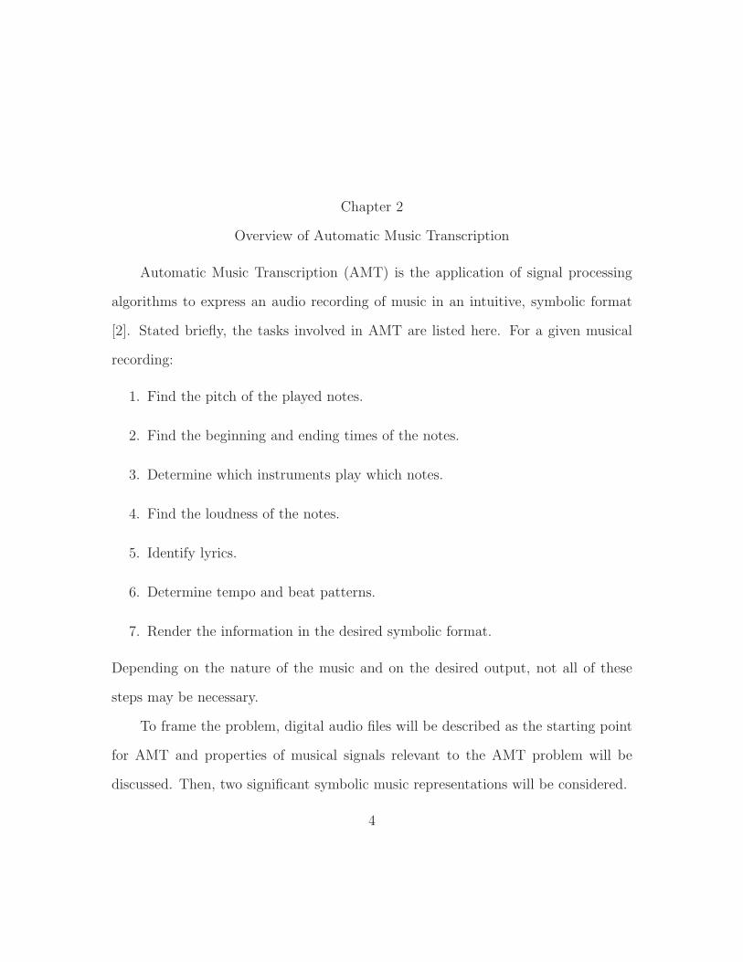
Automatic Music Transcription (AMT) is the application of signal processing
algorithms to express an audio recording of music in an intuitive, symbolic format
[2]. Stated briefly, the tasks involved in AMT are listed here. For a given musical
recording:
1. Find the pitch of the played notes.
2. Find the beginning and ending times of the notes.
3. Determine which instruments play which notes.
4. Find the loudness of the notes.
5. Identify lyrics.
6. Determine tempo and beat patterns.
7. Render the information in the desired symbolic format.
Depending on the nature of the music and on the desired output, not all of these
steps may be necessary.
To frame the problem, digital audio files will be described as the starting point
for AMT and properties of musical signals relevant to the AMT problem will be
discussed. Then, two significant symbolic music representations will be considered.
4
2.1 Digital Audio Files
AMT begins with a digital audio recording of music, which in its most common
forms is nothing more than the data recorded on an audio compact disc (CD) or,
more recently, the data downloaded from various online stores in compressed formats
(e.g., MP3, AAC, and WMA). These files document the movements of a microphone
diaphragm excited by sound pressure waves produced during a musical performance.
Since the changes in diaphragm position are recorded over time, this is naturally a
time domain format. The recorded movements are later reproduced in headphones
and car stereos for the enjoyment of the listener.
CD quality audio is a standard, uncompressed format using pulse-code modu-
lated (PCM) data sampled at a rate of 44.1 kHz with 16 bits used for each sample.
Two channels are recorded to mimic the binaural nature of human hearing. The 44.1
kHz offers a Nyquist frequency of 22.05 kHz, more than satisfying the demands of
the human ear, which responds to tones from roughly 20 Hz to 20 kHz, and 16 bits
afford a considerable dynamic range. Compressed formats take steps to reduce file
sizes by encoding only the more important elements in the musical signal. Generally,
this importance is determined by psychoacoustics, or the study of humans’ percep-
tion of sound. Compressed formats can vary widely in quality, depending on the
amount of compression and the techniques used. MP3 at a constant bit rate of 64
kbps will exhibit noticeable distortion in comparison with an uncompressed original.
Mostly, however, modern compression schemes are quite good, and MP3 at 320 kbps
can be difficult, if not impossible, to distinguish from CD quality, especially without
good stereo equipment. Further information on audio coding practices can be found
5
in [3]. In this thesis, all data examples are recorded at CD quality, but a point of
concern for AMT is that if an AMT algorithm is reliant on information which a given
compression scheme deems unimportant to the human ear, such an algorithm may
suffer when operating on compressed data.
2.2 Considerations on the Nature of Musical Signals
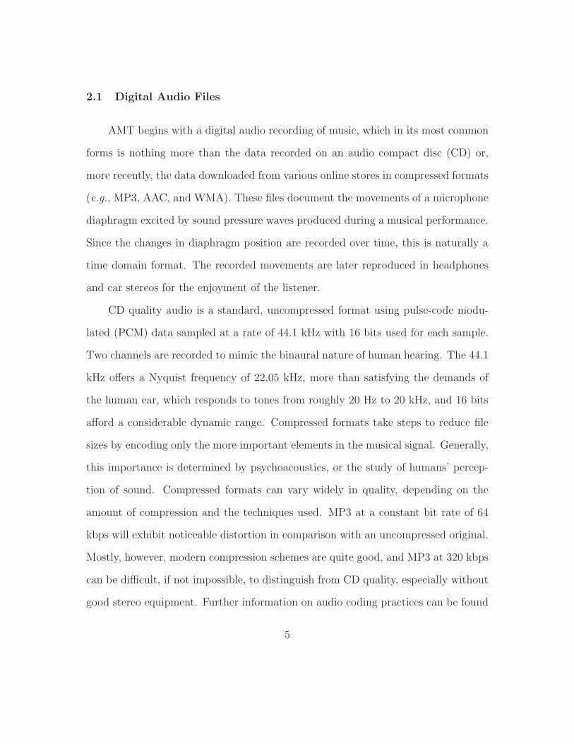
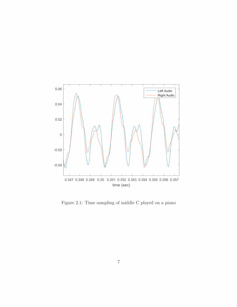
Figure 2.1 shows a small fraction of the audio samples recorded upon striking
the middle C piano key (C4 in scientific notation with a fundamental frequency of
approximately 261.6 Hz). Evident is the complex nature of the tone, with visible
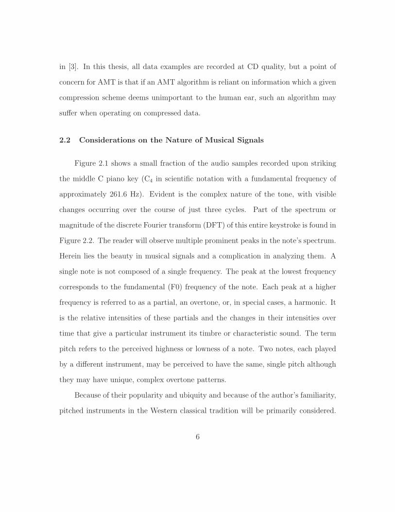
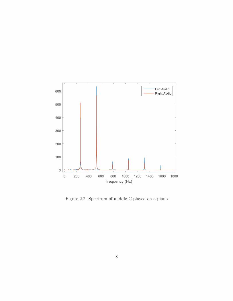
changes occurring over the course of just three cycles. Part of the spectrum or
magnitude of the discrete Fourier transform (DFT) of this entire keystroke is found in
Figure 2.2. The reader will observe multiple prominent peaks in the note’s spectrum.
Herein lies the beauty in musical signals and a complication in analyzing them. A
single note is not composed of a single frequency. The peak at the lowest frequency
corresponds to the fundamental (F0) frequency of the note. Each peak at a higher
frequency is referred to as a partial, an overtone, or, in special cases, a harmonic. It
is the relative intensities of these partials and the changes in their intensities over
time that give a particular instrument its timbre or characteristic sound. The term
pitch refers to the perceived highness or lowness of a note. Two notes, each played
by a different instrument, may be perceived to have the same, single pitch although
they may have unique, complex overtone patterns.
Because of their popularity and ubiquity and because of the author’s familiarity,
pitched instruments in the Western classical tradition will be primarily considered.
6
0.347 0.348 0.349 0.35 0.351 0.352 0.353 0.354 0.355 0.356 0.357time (sec)
-0.04
-0.02
0
0.02
0.04
0.06 Left AudioRight Audio
Figure 2.1: Time sampling of middle C played on a piano
7
0 200 400 600 800 1000 1200 1400 1600 1800frequency (Hz)
0
100
200
300
400
500
600Left AudioRight Audio
Figure 2.2: Spectrum of middle C played on a piano
8
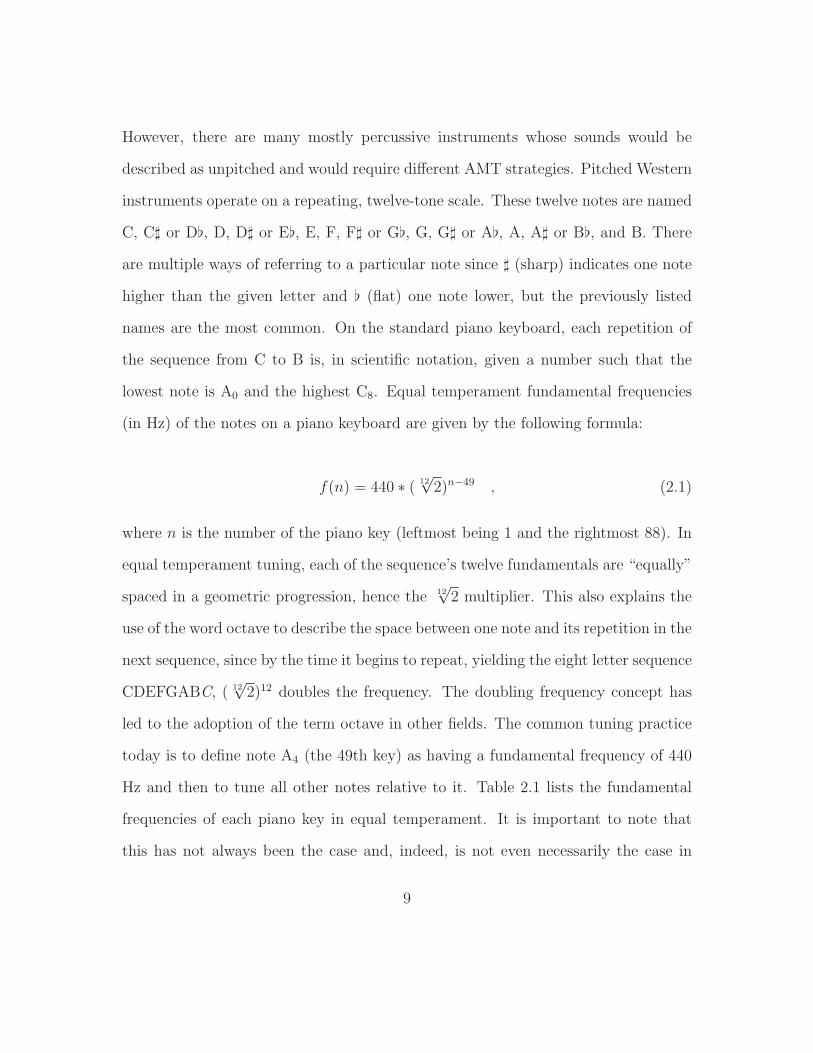
However, there are many mostly percussive instruments whose sounds would be
described as unpitched and would require different AMT strategies. Pitched Western
instruments operate on a repeating, twelve-tone scale. These twelve notes are named
C, C� or D�, D, D� or E�, E, F, F� or G�, G, G� or A�, A, A� or B�, and B. There
are multiple ways of referring to a particular note since � (sharp) indicates one note
higher than the given letter and � (flat) one note lower, but the previously listed
names are the most common. On the standard piano keyboard, each repetition of
the sequence from C to B is, in scientific notation, given a number such that the
lowest note is A0 and the highest C8. Equal temperament fundamental frequencies
(in Hz) of the notes on a piano keyboard are given by the following formula:
f(n) = 440 ∗ ( 12√2)n−49 , (2.1)
where n is the number of the piano key (leftmost being 1 and the rightmost 88). In
equal temperament tuning, each of the sequence’s twelve fundamentals are “equally”
spaced in a geometric progression, hence the 12√2 multiplier. This also explains the
use of the word octave to describe the space between one note and its repetition in the
next sequence, since by the time it begins to repeat, yielding the eight letter sequence
CDEFGABC, ( 12√2)12 doubles the frequency. The doubling frequency concept has
led to the adoption of the term octave in other fields. The common tuning practice
today is to define note A4 (the 49th key) as having a fundamental frequency of 440
Hz and then to tune all other notes relative to it. Table 2.1 lists the fundamental
frequencies of each piano key in equal temperament. It is important to note that
this has not always been the case and, indeed, is not even necessarily the case in
9
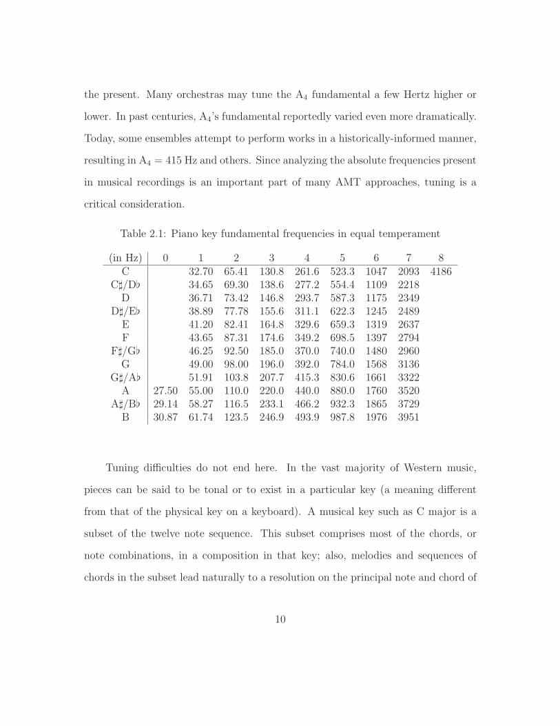
the present. Many orchestras may tune the A4 fundamental a few Hertz higher or
lower. In past centuries, A4’s fundamental reportedly varied even more dramatically.
Today, some ensembles attempt to perform works in a historically-informed manner,
resulting in A4 = 415 Hz and others. Since analyzing the absolute frequencies present
in musical recordings is an important part of many AMT approaches, tuning is a
critical consideration.
Table 2.1: Piano key fundamental frequencies in equal temperament
(in Hz) 0 1 2 3 4 5 6 7 8C 32.70 65.41 130.8 261.6 523.3 1047 2093 4186
C�/D� 34.65 69.30 138.6 277.2 554.4 1109 2218D 36.71 73.42 146.8 293.7 587.3 1175 2349
D�/E� 38.89 77.78 155.6 311.1 622.3 1245 2489E 41.20 82.41 164.8 329.6 659.3 1319 2637F 43.65 87.31 174.6 349.2 698.5 1397 2794
F�/G� 46.25 92.50 185.0 370.0 740.0 1480 2960G 49.00 98.00 196.0 392.0 784.0 1568 3136
G�/A� 51.91 103.8 207.7 415.3 830.6 1661 3322A 27.50 55.00 110.0 220.0 440.0 880.0 1760 3520
A�/B� 29.14 58.27 116.5 233.1 466.2 932.3 1865 3729B 30.87 61.74 123.5 246.9 493.9 987.8 1976 3951
Tuning difficulties do not end here. In the vast majority of Western music,
pieces can be said to be tonal or to exist in a particular key (a meaning different
from that of the physical key on a keyboard). A musical key such as C major is a
subset of the twelve note sequence. This subset comprises most of the chords, or
note combinations, in a composition in that key; also, melodies and sequences of
chords in the subset lead naturally to a resolution on the principal note and chord of
10
the key. The aesthetically pleasing consonances of these chords and their sequences
led to the conventional recognition of keys in music theory. The rub lies in the fact
that equal temperament tuning does not produce the highest degree of consonance
in the chords of a particular key. Equal temperament tuning is a compromise which
permits reasonable approximations to ideal consonance to be produced in all possible
musical keys. This practice dramatically increases the musical flexibility of keyboard
instruments such as the piano, which if tuned to achieve ideal consonance in a par-
ticular key, could not (at least with blessing from the audience) employ certain keys
or certain types of chords. Tuning a piano is time-consuming and certainly could not
be done mid-performance. Where this impacts AMT is not with pianos, but other
instruments. While the pianist does not have real-time control over his instrument’s
tuning, all brass, woodwind, and most string instrumentalists do, with some having a
greater extent of control than others. For this reason, orchestras and other ensembles
using only such instruments will many times alter the tuning of individual notes in
pursuit of the ideal consonance as the chords progress and the key changes within a
given piece. In short, the “best” (ideal consonance) tuning of E4, for instance, is not
the same in all chords; musicians regard this fact and adjust accordingly if context
permits.
This naturally leads to the subject of variation among instrumental sounds.
A pianist is somewhat limited in the sounds he can produce on a single instrument
(though one piano can sound quite different from another). When the hammer strikes
the string, there is a rapid onset of the string’s vibration which then slowly dies away.
The pianist can either wait, re-strike the note, or end its vibration prematurely.
11
Apart from what control the initial velocity of the hammer provides, the string
vibrates as it will. This is quite different from other instruments whose notes are
produced and sustained only by the musician’s continued effort. Brass, woodwind,
and orchestral string instruments have the power to begin notes quite softly and
increase their volumes over their durations. In addition to this, these musicians
can alter the timbres of their instruments considerably. The violinist can produce
a sweet, melodic sound or a rougher, more aggressive sound by an alteration of
the bowing technique. Also, the orchestral strings are routinely plucked, producing
yet a different sound. They can also, along with trombones, employ a glissando—a
perfectly smooth bending of the pitch from one note to another, often across many
notes. In this technique, the discrete nature of the intervening notes is completely
ignored. Varying styles also prompt varying sounds. A lead trumpet player in a
jazz ensemble will produce quite a different sound from an orchestral trumpeter.
Depending on the scope of the problem, AMT algorithms will have to account for
such things. [4] provides an excellent reference on a wide range of instruments from
a physics standpoint.
Since the piano is prominent in this thesis, another note on piano tuning will
be considered. The reader may have noticed the apparently even spacing of the
peaks in the spectrum of the piano tone. In this special case, the fundamental and
partials are referred to as harmonics. Each peak is located at a frequency which is
an integer multiple of the fundamental frequency. This results due to the physics
of a vibrating string—at least, of an ideal string. Piano strings are made of steel
(with bass strings wound with copper to increase mass) and have a certain amount
12
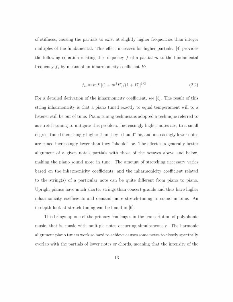
of stiffness, causing the partials to exist at slightly higher frequencies than integer
multiples of the fundamental. This effect increases for higher partials. [4] provides
the following equation relating the frequency f of a partial m to the fundamental
frequency f1 by means of an inharmonicity coefficient B:
fm ≈ mf1[(1 +m2B)/(1 + B)]1/2 . (2.2)
For a detailed derivation of the inharmonicity coefficient, see [5]. The result of this
string inharmonicity is that a piano tuned exactly to equal temperament will to a
listener still be out of tune. Piano tuning technicians adopted a technique referred to
as stretch-tuning to mitigate this problem. Increasingly higher notes are, to a small
degree, tuned increasingly higher than they “should” be, and increasingly lower notes
are tuned increasingly lower than they “should” be. The effect is a generally better
alignment of a given note’s partials with those of the octaves above and below,
making the piano sound more in tune. The amount of stretching necessary varies
based on the inharmonicity coefficients, and the inharmonicity coefficient related
to the string(s) of a particular note can be quite different from piano to piano.
Upright pianos have much shorter strings than concert grands and thus have higher
inharmonicity coefficients and demand more stretch-tuning to sound in tune. An
in-depth look at stretch-tuning can be found in [6].
This brings up one of the primary challenges in the transcription of polyphonic
music, that is, music with multiple notes occurring simultaneously. The harmonic
alignment piano tuners work so hard to achieve causes some notes to closely spectrally
overlap with the partials of lower notes or chords, meaning that the intensity of the
13
partials in the frequency domain, rather than their mere presence, may be the only
clue that those notes are being played. For more on this, see Chapter 5.
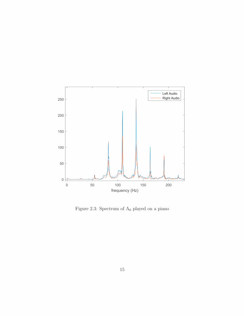
A further curiosity of pianos can be found in the spectra of the extremely low
notes. The fundamentals of these notes have surprisingly little presence in their
spectra in comparison with the higher-frequency partials, yet humans still perceive
the pitches of these notes to correspond with their fundamental frequencies. See
Figure 2.3 for the spectrum of piano note A0; the fundamental at approximately 27.5
Hz (this piano is stretch-tuned) is only barely visible next to the far more prominent
higher-frequency partials. For a detailed look at piano physics which includes a good
introductory treatment of the missing fundamental, see [7].
The importance of piano string inharmonicity, stretch-tuning, and missing fun-
damentals to AMT is that while the piano on its face may seem tame for spectral
analysis purposes with nicely predetermined, unchanging frequencies and limited tim-
bral variation, creating an algorithm to account for the tuning and partial-presence
variations of pianos in general is no mean feat. While the brain is quite good at
recognizing that a cheap upright piano and a world-class concert grand are still both
in fact pianos, their spectral properties will differ markedly.
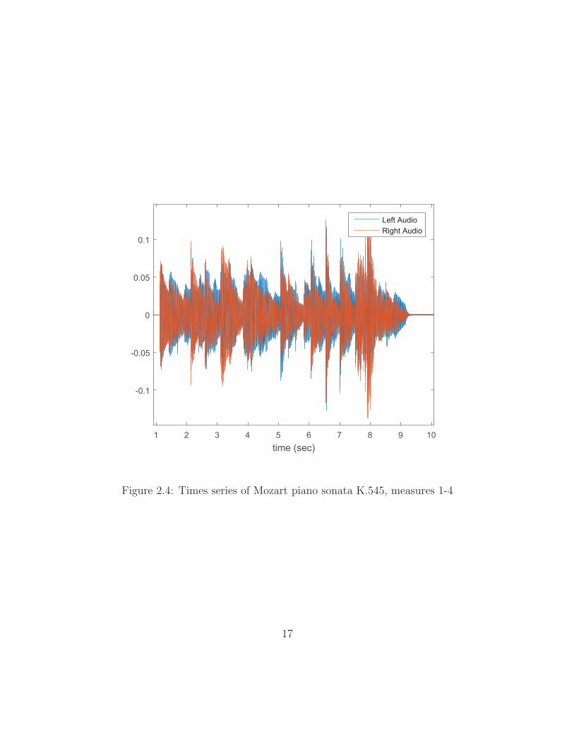
To provide better visualization of a musical signal in context, the beginning of
Mozart’s Piano Sonata K.545 will be considered. Figure 2.4 shows the left and right
audio channels for the first 10 seconds of the piece. The look is characteristic of
piano recordings because of the sudden increases in energy as notes are struck and
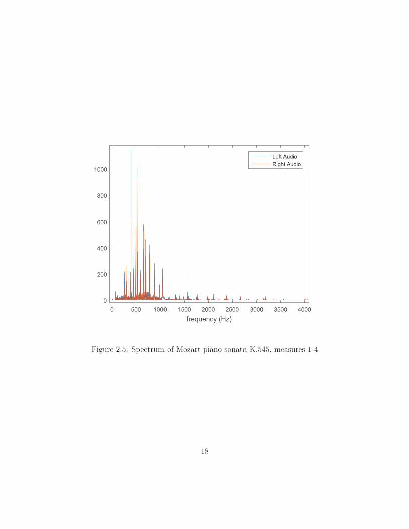
gradual decreases as the notes decay. Figure 2.5 shows the spectrum of the same
10 seconds of recording. Since the time information is not clearly discernible in this
14
0 50 100 150 200frequency (Hz)
0
50
100
150
200
250Left AudioRight Audio
Figure 2.3: Spectrum of A0 played on a piano
15
domain, all the notes’ spectra are overlapping in this figure, regardless of when the
notes occur. For this reason, the short-time Fourier transform (STFT) provides a
good means of envisioning musical signals, which have changes of interest occurring
in both the time and frequency domains. It amounts to merely calculating a series of
short DFTs on windowed portions of the entire signal with the goal of highlighting
the change in the spectrum over time. [8] provides the following definition for the
STFT of a signal x[n]:
XSTFT [k, lL] = XSTFT (ej2πk/N , lL) =
R−1∑m=0
x[lL−m]w[m]e−j2πkm/N , (2.3)
where l is an integer such that −∞ < l < ∞ and k is an integer such that 0 ≤ k ≤N − 1. L is the number of samples that the length-R window function w[n] shifts
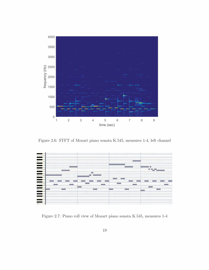
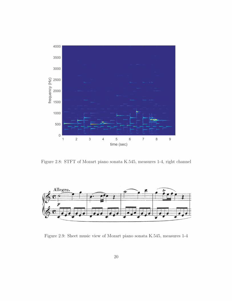
for each DFT of N frequency samples. Figure 2.6 contains an STFT of the Mozart
recording’s left audio channel, and Figure 2.8 contains the right. These STFTs
use a step size of L = 300 samples (≈ 6.8 ms) and a Hanning window of length
R = 5000 samples (≈ 0.11 s). This proves an excellent starting point for visualizing
musical signals. [9] treats the STFT at length, considering different windows, with
applications tailored to audio signal processing.
16
1 2 3 4 5 6 7 8 9 10time (sec)
-0.1
-0.05
0
0.05
0.1
Left AudioRight Audio
Figure 2.4: Times series of Mozart piano sonata K.545, measures 1-4
17
0 500 1000 1500 2000 2500 3000 3500 4000frequency (Hz)
0
200
400
600
800
1000
Left AudioRight Audio
Figure 2.5: Spectrum of Mozart piano sonata K.545, measures 1-4
18
1 2 3 4 5 6 7 8 9time (sec)
0
500
1000
1500
2000
2500
3000
3500
4000
frequ
ency
(Hz)
Figure 2.6: STFT of Mozart piano sonata K.545, measures 1-4, left channel
Figure 2.7: Piano roll view of Mozart piano sonata K.545, measures 1-4
19
1 2 3 4 5 6 7 8 9time (sec)
0
500
1000
1500
2000
2500
3000
3500
4000fre
quen
cy (H
z)
Figure 2.8: STFT of Mozart piano sonata K.545, measures 1-4, right channel
Figure 2.9: Sheet music view of Mozart piano sonata K.545, measures 1-4
20
2.3 Symbolic Music Representations
The end goal is to take the musical recording and render it in a useful symbolic
format. While there are many possibilities, two primary ones with their advantages
and disadvantages will be considered here due to their intuitiveness and commonness.
The first is the “piano roll” format. It is quite common in musical instrument
digital interface (MIDI) software. MIDI provides a highly condensed format for
storing sequences of musical notes and has been for many years a popular interface
between electronic instruments and computers [10]. MIDI files do not store any actual
audio data, but merely the pitch, onset time, release time, attack velocity, and other
data concerning each note. When MIDI files are played back to a listener, a computer
consults a collection of audio tones from different instruments and constructs an audio
recording. The piano roll is an intuitive way of viewing such data. A piano keyboard
is drawn along the left axis and time proceeds to the right. Whenever a note is used,
it receives a bar indicating its duration in the row of that note. Figure 2.7 provides
an example of this view using the previous Mozart excerpt for content. The note
input was done by exact specification in a computer and was not recorded in MIDI
format by performance on a MIDI instrument.
The reader can observe the related patterns in Figure 2.7 and in Figures 2.6 and
2.8. The fundamental frequencies in the STFT images should roughly line up with
the notes indicated in the piano roll. The difference is, of course, that the vertical
axes have different scales. The keys on the piano roll are all equally spaced, but the
fundamental frequencies of those notes are spaced in a geometric series as shown in
Equation 2.1.
21
The advantage of the piano roll format is that the human element introduced by
a musical performance need not be removed. The human element in consideration
here is probably best captured by the musical term rubato, which refers to expressive
quickening and slowing of the tempo at the discretion of the performer. Many types
of music employ this element liberally. The result of this is that the times which the
notes occur are not readily aligned in the structured pattern of beats necessary in
the next symbolic format, namely sheet music. Figure 2.9 shows the same collection
of notes rendered in standard musical notation [11]. The same pattern of content is
visible in this figure.
Musical notation documents a series of music notes by casting them on and
between horizontal lines. Time progresses to the right until the page ends, and then
a new set of lines is begun. Pitch is denoted by vertical position on the lines. Notes
are represented by ovals and their durations are shown by whether they are filled in
and by the number of tails or bars they have. The vertical lines separate measures
(collections of beats in the piece), and each measure has a strictly set number of
beats which progress at a speed indicated at the outset—in this case, allegro (fast).
Rubato causes beats not to occur at always the same intervals of time, meaning one
measure may be longer in seconds than another. Finding the onset time of a note in
seconds from the beginning of the recording is one thing, but determining the beat
and measure in which it occurs is a different matter entirely, since the progression of
beats may have no correlation to the progression of seconds. To achieve a sensible
representation of a recording in musical notation, extra steps must be performed
such as beat tracking and quantization of note onset times to particular beats. Also,
22
a sensible decision (likely informed by music theory) must be made concerning the
grouping of beats into measures. A musician will say these groupings are arbitrary
to an extent, but taste must be exercised to produce a readable musical score.
The reader may have noticed that the piano roll also indicates measure divisions,
and indeed, MIDI records beats and measures. However, a user can easily ignore
MIDI’s beat and measure structure and operate solely in terms of seconds with little
ill effect on the piano roll visualization. The result of a similar disregard in musical
notation is difficult to interpret and not generally useful. In short, the piano roll is a
reasonable way of looking at an AMT result but is not easily readable by a musician
for re-performance. Musical notation is far more accessible to the musician, but
creating such a score requires removing the human element in the recording, which
is no easy task. [12] can be consulted as an introduction to musical notation and
music theory in general.
23
Chapter 3
Problem Considered in This Thesis
To keep the problem of AMT tractable for the purposes of this thesis, several
restrictions are imposed. First, only recordings of pianos will be used as input data.
This removes the need to differentiate between various instruments. This also simpli-
fies the problem of note onset detection since piano notes all have a decisive beginning
with the hammer striking the string. Originally, the proposed algorithm was going
to attempt modeling pianos in general, allowing a recording of any piano to be an-
alyzed. The significant variability (detailed in Section 2.2) of tuning and partials
among pianos makes far more extensive research and mathematical efforts necessary
to achieve an acceptable result. As a compromise, the algorithm will be permitted a
calibration signal—simply a recording of the playing of every key in order, one at a
time, from A0 to C8. Ideally, each note of this signal will be approximately 2 seconds
long, and notes will be separated by silence. For the best results, the calibration
signal should be updated if the music to be transcribed is played on a different piano
or if the recording equipment or setup changes. The algorithm will create a library of
spectral data which it will consult when performing multiple fundamental frequency
estimation.
Unless otherwise stated, the data depicted in this thesis is a recording of a
Roland RD-700GX digital stage piano on the Expressive Grand setting, and the
24
recordings were collected using a Sony PCM-M10 Portable Linear PCM Recorder.
A stereo cable connected the digital keyboard directly to the recorder, avoiding
ambient noise. Ground truth was collected by simultaneously recording the sequence
of piano keystrokes in MIDI format. The designers of this keyboard seem to have
taken considerable pains to realistically reproduce the sound of a grand piano. The
notes are sampled from a real piano, and even such subtleties as damper noise and
sympathetic vibration of strings have been taken into account.
The two questions primarily considered for a given recording are:
• When does each note begin?
• What is the pitch of each note?
The removal of the human element (described in Section 2.3) and the production
of a transcription in musical notation is not attempted. The determination of the
volume of each note is treated only indirectly as a consequence of note detection.
The product of the suggested algorithm will mimic the piano roll visualization for
easy comparison with the ground truth.
25
Chapter 4
Note Onset Detection
Note onset detection is the problem of pinpointing the beginnings of notes in
musical recordings. More generally, onset detection may be applied to unpitched or
percussive sounds in music which might not be strictly considered notes. The im-
portance is straightforward. If an algorithm can identify the instants in time when
new spectral content is appearing in a medium like music, which is fundamentally
time-frequency based, a significant step has been made in breaking down the struc-
ture of the recording. First, a brief review of note onset detection approaches will be
conducted, then the specific strategy applied in this thesis will be described.
4.1 Review of Approaches
One of the simpler approaches to onset detection focuses on the occurrence of
transient events at the beginning of unpitched percussive sounds and some pitched
sounds like those of the piano, guitar, and percussion instruments like chimes, marim-
bas, or timpani. These transient events are characterized by sudden increases in
spectral energy and can be highlighted by merely summing energy in each step of
the STFT as described in [2].
E(n) =∑k
|XSTFT (k, n)|2 . (4.1)
26
Looking for peaks in E or rapid changes in E will help find the peak power of the
transients or their beginnings and thus the note onsets associated with them. Such
a method works tolerably for pianos since transients accompany their notes, but
improvements can be made that capitalize on the piano as a pitched instrument.
[13] describes finding vector distances between successive spectral frames of the
STFT for a subtler observation of the spectral change. The authors of that paper list
a few ways of calculating such a vector distance, beginning with a simple Euclidean
distance, and propose the modified Kullback-Liebler distance dn(k) as the best.
dn(k) = log2
( |XSTFT (k, n)||XSTFT (k, n− 1)|
). (4.2)
At this point, summing dn over k and looking for changes in the resulting function
will produce better results than Equation 4.1, since a change in frequency content—
even in the absence of a change in total energy—will be visible. In fact, this was
the primary motivation for this step. Many instruments, including the human voice,
can employ a soft onset and smooth changes without any hint of a transient rise
in energy. Note changes in choirs and string quartets are thus far more difficult to
detect. A further improvement is to sum only the positive elements of dn since the
addition, rather than the departure, of spectral energy is of interest. Also, [14], [15],
and others suggest weighting certain frequency bands more heavily or considering
only certain bands based on the content sought.
A good overview and comparison of note onset detection methods, including
wavelet and phase-based approaches, can be found in [16]. These authors point out
that accounting for the imaginary part of the spectrum, too, rather than merely
27
the magnitude is important because of the time information encoded in the phase.
Wavelet methods show the potential for providing a precise onset estimation. More
recently, [17] uses the L2-norm to calculate distances between spectral vectors and
adds a subsequent time-domain process to refine the onset estimation of percussive
sounds. [18] makes a good observation about the false alarms caused by musical
techniques such as vibrato—a small, repeated fluctuation in the pitch and intensity
of a note—and suggests a pitch salience function which is then smoothed to reduce
the effect of such fluctuations. Attempts are being made to treat both pitched and
unpitched sounds with the same algorithm as in [19]. Finally, [20] offers a neural
network approach operating only on causal audio information.
4.2 Suggested Approach
Many of the authors in the previous section analyzed recordings with multiple
instruments prompting more complex approaches. For the comparatively simpler
problem of piano-only onset detection, this author has found a spectral change func-
tion using a mere vector difference (also used in [21]), rather than the more sophisti-
cated L2-norm or modified Kullback-Liebler distance, to be computationally fast and
effective. This is followed by a heuristically-tailored peak-picking step to pinpoint
onsets. The equations describing the operation of the algorithm are:
dn(k) = |XSTFT (k, n)| − |XSTFT (k, n− 1)| , (4.3)
and
28
Ds(n) =∑
k,dn>0
dn(k) . (4.4)
This spectral rise function Ds is calculated for both the left and right audio
channels in the recording, and the results are fused using a point-wise average, i.e.,
Ds,total(n) =Ds,left(n) +Ds,right(n)
2. (4.5)
Now, peak-finding is applied to resolve note onsets, and several steps are taken as
mentioned in [2] to remove false alarms. Particularly strong onsets, usually indicative
of large, loud chords, often have fluctuations in spectral energy as the transient dies
away, resulting in low-scoring, false alarm onsets. Heuristic thresholds are set to
minimize such issues. See Section 6.1 for a more detailed description with example
figures.
29

Chapter 5
Multiple Fundamental Frequency Estimation
Multiple fundamental frequency estimation is a critical part of AMT since a
very large portion of music today is polyphonic. This results in entwined spectral
content in analysis windows of multiple notes, and many times, in the case of oc-
taves and other particular intervals, the partials of the notes will overlap to a high
extent. Identifying each of the simultaneous notes is necessary to producing an ac-
curate transcription. If an algorithm can estimate which spectral components are
the fundamentals when presented with a signal composed of multiple overtones and
fundamentals, then it will have identified the pitches in the signal. Following is a
review of current approaches and then a description of the method applied to the
problem at hand.
5.1 Review of Approaches
Many different methods have been proposed for solving the multiple fundamental
estimation problem. [2] divides the approaches into three large groups and provides a
good overview of the progress up to the publication in 2006. The first main category
the authors treat is one based on generative models, which are then subjected to
a probabilistic analysis. The models are designed to reflect the nature of the pro-
duction of polyphonic music. A piano, for instance, has equations which attempt to
30
describe the frequencies of the fundamentals of each note and the frequencies of the
overtones (see Section 2.2). Since not all pianos will be tuned the same way or have
the same spectral properties, estimations may be made ahead of time concerning the
distribution of such values for pianos in general, e.g., picking the most likely tuning
of a piano and applying a Gaussian distribution to allow for variation. A probabilis-
tic estimation, such as minimizing the mean squared error, then suggests the most
likely model parameters to explain the given waveform. These models can become
quite complicated, but a relatively simple example is the sum-of-sines model—not
unreasonable for music signals, considering the nicely discrete spikes in the spectra.
This model is given in [2] by
x(n) =M∑
m=1
αs sin(2πmk1n) + αc cos(2πmk1n) , (5.1)
where m is the partial number and αs, αc, and k1 are estimated to match a given
input signal. Approaches like these are attractive since they offer the possibility of
accounting for much of the physics involved in the production of music. The result
will only be as good as the model, however, and such approaches can quickly become
computationally expensive.
More recently, [21] proposes a genetic algorithm using a model that adapts the
spectral envelopes of previously recorded piano samples. A method is suggested in
[22] to deal with the octave partials overlap problem by a different spectral model
considering even and odd partials separately. [23] considers a piano-specific gener-
ative model for the transcription problem. As an aside, it is worth noting that the
31
term source separation is sometimes used to describe the multiple fundamental fre-
quency problem. Though source separation is perhaps first motivated by identifying
the contributions of two or more different sources of sound (e.g., different instruments
in music or voices in speech) in a recording, the issues involved are essentially the
same as those in identifying the contributions of two or more different strings in a
single piano.
The second major category involves an extension of monophonic fundamental
estimation techniques. These operate intuitively by attempting to gauge the peri-
odicity of the music signal in either the time domain or the frequency domain with
an autocorrelation or similar function. The extension involves merely a repetition of
the monophonic method. Either a signal is repeatedly built up with tones until it
matches the input signal, or tones are subtracted repeatedly from the input signal
until it is fully explained (see [24]). With the latter, care must be taken to prevent
spoiling of tones which may have spectral content overlapping that of a subtracted
tone. [2] highlights the addition of models based on the human auditory system to
enhance these techniques. Since the goal is to determine the way a complex spectrum
maps to pitch and timbre, it may be useful to consider the human brain’s tactics,
as it accomplishes the task quite readily. A nice introduction to auditory perception
can be found in [25], and [26] offers more details about the application of such a
model to the AMT problem.
Several later efforts have focused on this second category. [27] takes an approach
of a weighted summing of narrowband spectra which are adapted based on the spec-
tral envelopes of various instruments. [28] focuses on the piano and assumes that the
32
spectral magnitude of a polyphonic signal can be described as a linear combination
of the spectral magnitudes of a dictionary of piano tones. The authors take note
of different types of piano spectra—those where the fundamental is the strongest
spectral peak and those where an overtone is more intense than the fundamental.
Both [28] and [29] rely on sparsity in formulating their solutions. [30] proposes the
utilization of the note temporal evolution in a consulted dictionary of piano notes
and proposes a new psychoacoustic measure.
The final large category is that of unsupervised learning methods. The idea is
that when fed a great deal of data, an algorithm may be able to perform source
separation by recognizing patterns which are not readily apparent. Some recent
publications using unsupervised approaches include [31], [32], and [33].
5.2 Suggested Approach
The approach taken in this thesis attempts to combine a set of piano tones from
a pre-recorded dictionary (the calibration signal described in Chapter 3) to match a
given spectrum of interest. Virtanen observes in Chapter 9 of [2] that when multiple
sources simultaneously sound, their individual acoustic waveforms add linearly. Since
the DFT is a linear operation, the DFTs of such individual acoustic waveforms will
add linearly. That is, if
x(n) → X(k) , (5.2)
ym(n) → Ym(k) , (5.3)
33
where X(k) and Ym(k) are the respective DFTs of a polyphonic time signal x(n) and
its monophonic components ym(n), then
x(n) =∑m
ym(n) , (5.4)
X(k) =∑m
Ym(k) . (5.5)
However, X(k) and Ym(k) are complex and
|X(k)| �=∑m
|Ym(k)| . (5.6)
This seems problematic, since the magnitude of the DFT is a common and useful way
of dealing with spectral information. For this application in particular, one would
have to be concerned with the phase information in the dictionary matching the
phase information in the input data when combining dictionary tones—an unlikely
situation. Virtanen points out, however, that, assuming the phases of Ya(k) and
Yb(k) are uniformly distributed and independent of each other for a �= b,
E{|X(k)|2} =∑m
|Ym(k)|2 , (5.7)
where E{·} is an expected value.
He writes that in spite of the consequence in Equation 5.6, the magnitude rep-
resentation has been used (as in [28]) and often with good results though a good
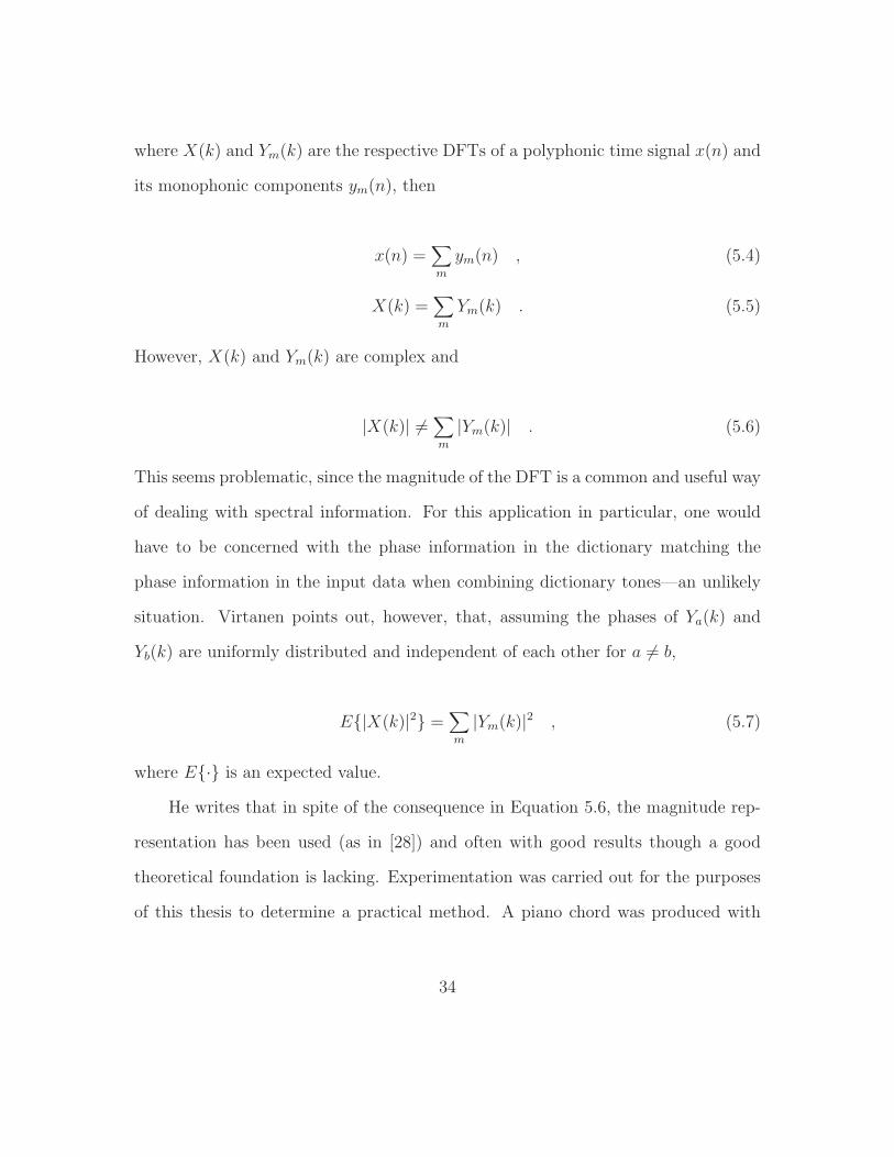
theoretical foundation is lacking. Experimentation was carried out for the purposes
of this thesis to determine a practical method. A piano chord was produced with
34
the notes A1, A2, E3, A3, C�4, E4, G4, and A4, which have a large percentage of
overlapping partials. The recording was produced with all notes being activated
with equal MIDI velocities, and subsequently each individual note of the chord was
played separately. The individual note spectra were then combined in three different
ways in an attempt to match the spectrum of the recorded entire chord. The first
utilizes Equation 5.7, the second sums directly (i.e., ignores Equation 5.6), and the
third takes the maximum spectral component of all the individual notes for any given
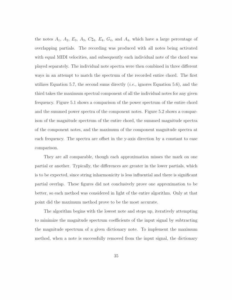
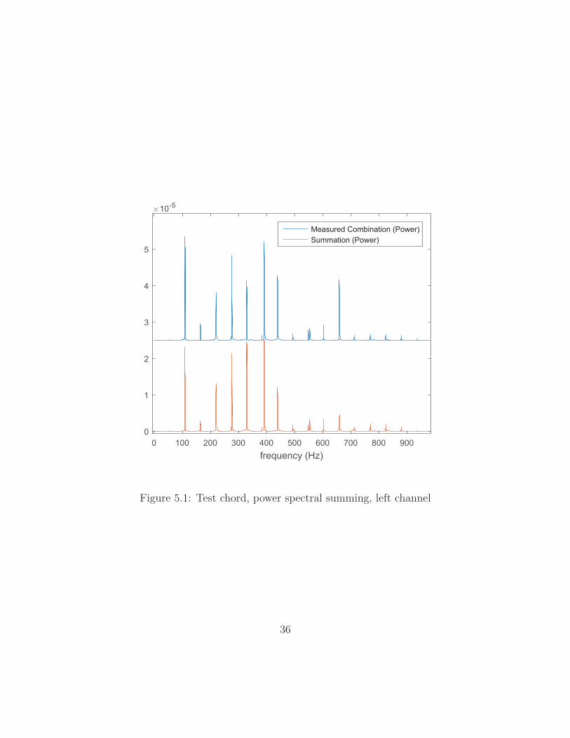
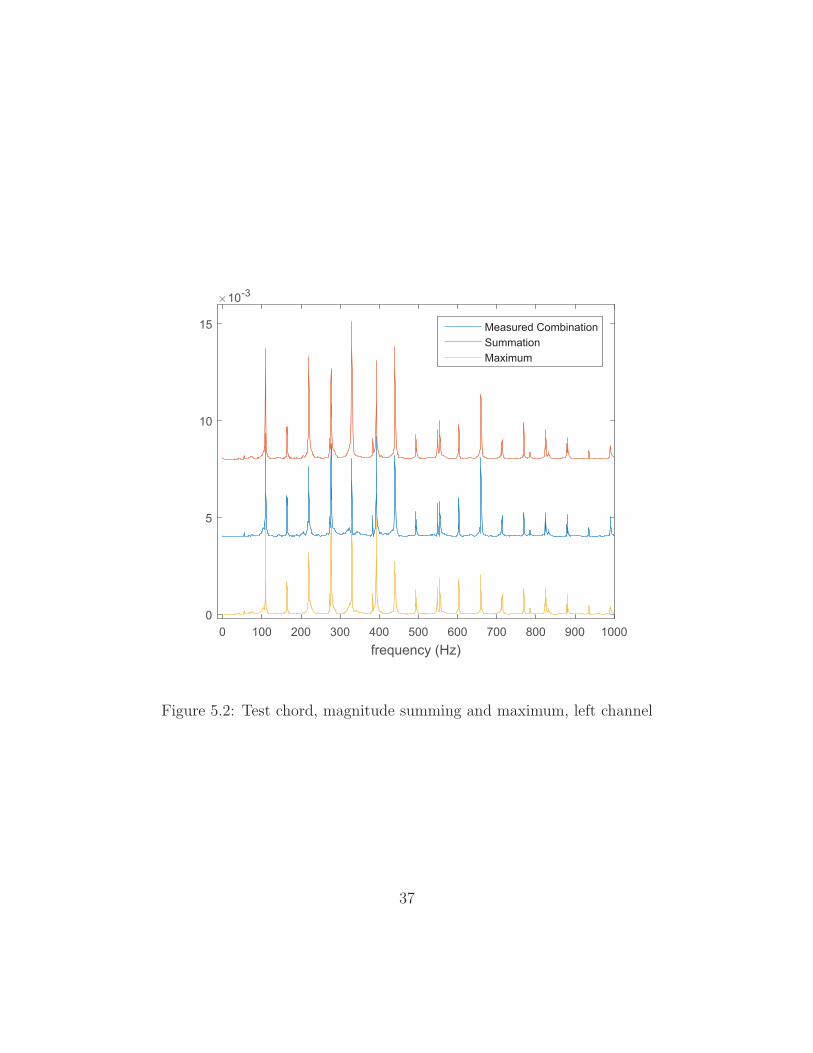
frequency. Figure 5.1 shows a comparison of the power spectrum of the entire chord
and the summed power spectra of the component notes. Figure 5.2 shows a compar-
ison of the magnitude spectrum of the entire chord, the summed magnitude spectra
of the component notes, and the maximum of the component magnitude spectra at
each frequency. The spectra are offset in the y-axis direction by a constant to ease
comparison.
They are all comparable, though each approximation misses the mark on one
partial or another. Typically, the differences are greater in the lower partials, which
is to be expected, since string inharmonicity is less influential and there is significant
partial overlap. These figures did not conclusively prove one approximation to be
better, so each method was considered in light of the entire algorithm. Only at that
point did the maximum method prove to be the most accurate.
The algorithm begins with the lowest note and steps up, iteratively attempting
to minimize the magnitude spectrum coefficients of the input signal by subtracting
the magnitude spectrum of a given dictionary note. To implement the maximum
method, when a note is successfully removed from the input signal, the dictionary
35
0 100 200 300 400 500 600 700 800 900frequency (Hz)
0
1
2
3
4
5
10-5
Measured Combination (Power)Summation (Power)
Figure 5.1: Test chord, power spectral summing, left channel
36
0 100 200 300 400 500 600 700 800 900 1000frequency (Hz)
0
5
10
15
10-3
Measured CombinationSummationMaximum
Figure 5.2: Test chord, magnitude summing and maximum, left channel
37
spectra of all higher notes must also undergo the removal of that note. This allows
the modified dictionary spectra to reflect the expected remaining spectrum in the
input signal. The result of this is a more conservative subtraction of spectral content
than would occur in the summed magnitude approach. This author believes that
this more careful removal of information explains the better performance.
38

Chapter 6
Algorithm Description and Results
This section describes the function of the proposed algorithm in detail. The
algorithm can be roughly divided into two portions. The first performs note onset
detection with the goal of dividing the input signal into windows of time when no
note changes occur. The second portion takes the windows and performs multiple
fundamental frequency estimation to identify the notes occurring in that window. A
piano roll visualization is then produced. The input signal will be given by xl[n] and
xr[n], which will denote the left and right channels, respectively, of a time-series of
recorded piano music, sampled at 44.1 kHz with a 16-bit depth.
6.1 Note Onset Detection
First, an STFT is performed on each audio channel separately, resulting in
Xl[k, hL] and Xr[k, hL] (Equation 2.3). The step size L is 300 samples (≈ 6.8 ms),
and the Hanning window used in the STFT has length of 5000 samples (≈ 0.11
s). Other parameters were tested, but these seem to provide a good balance of
performance and execution speed. The magnitude of these STFTs are calculated,
then the first-order differences dl,h[k] and dr,h[k] are found along the time direction
(Equation 4.3). All negative differences are made zero since the interest is in the
addition of spectral energy, and the remaining positive differences are summed over
39
k or along the frequency dimension, producingDl[h] andDr[h] (Equation 4.4). These
are averaged point-wise, giving Dtotal[h] (Equation 4.5).
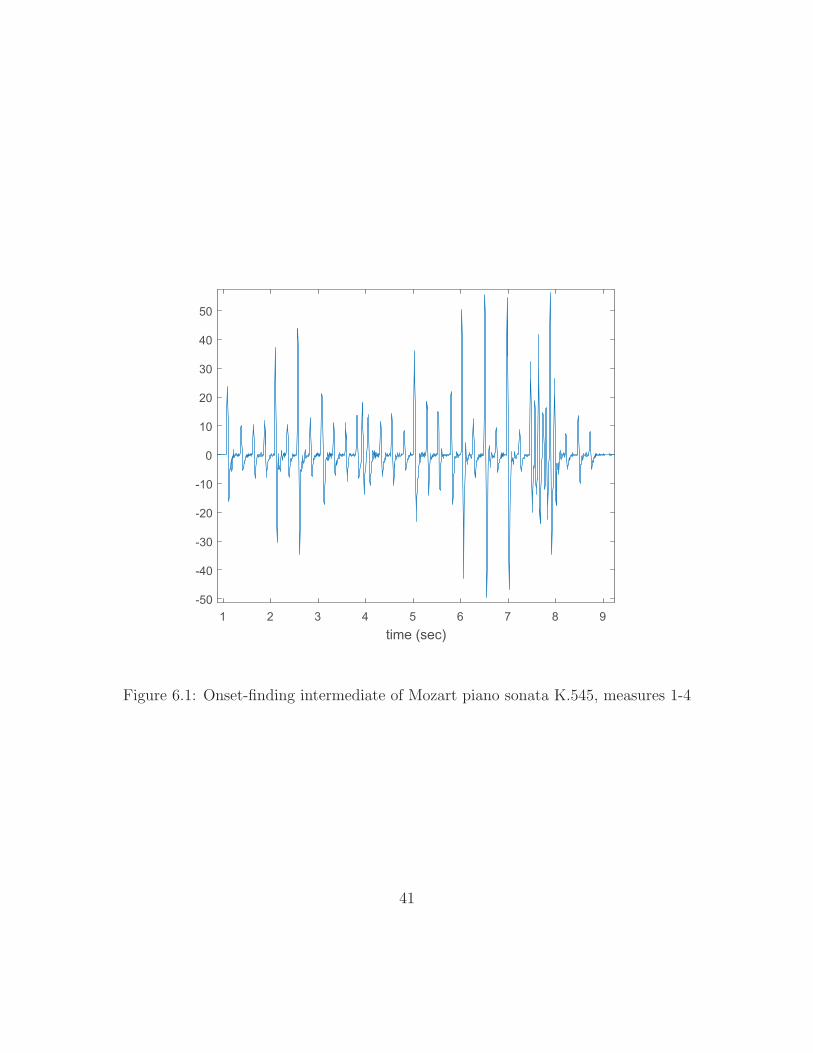
Now, a peak-finding step is used to pick out the times with the most rapid rises
in spectral energy, i.e., the percussive piano note onsets. The peak-finding operates
by finding the first order difference of Dtotal[h] and applying a score to every zero
crossing from positive to negative. The score is determined by the number and values
of consecutive positive differences immediately prior to the crossing and the number
and values of consecutive negative differences subsequent to the crossing. Figure 6.1
shows a plot of these differences using the Mozart sonata example from the earlier
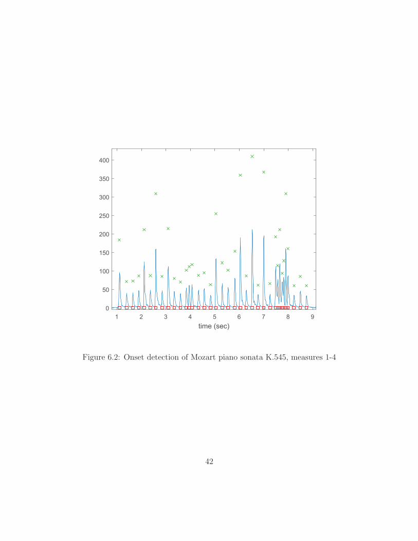
chapters. A filtering step then compares the relative scores and relative occurrence
times of the zero crossings and removes a weak score if it follows a high score too
closely. Large onsets tend to have fluctuations in the spectral energy as the attack
transient dies away; they can cause false alarms in onset detection. Figure 6.2 plots
Dtotal[h] for the Mozart example. Detected onsets are indicated by red squares and
the corresponding score of each is indicated by the vertical position of the green ‘x’
above the onset.
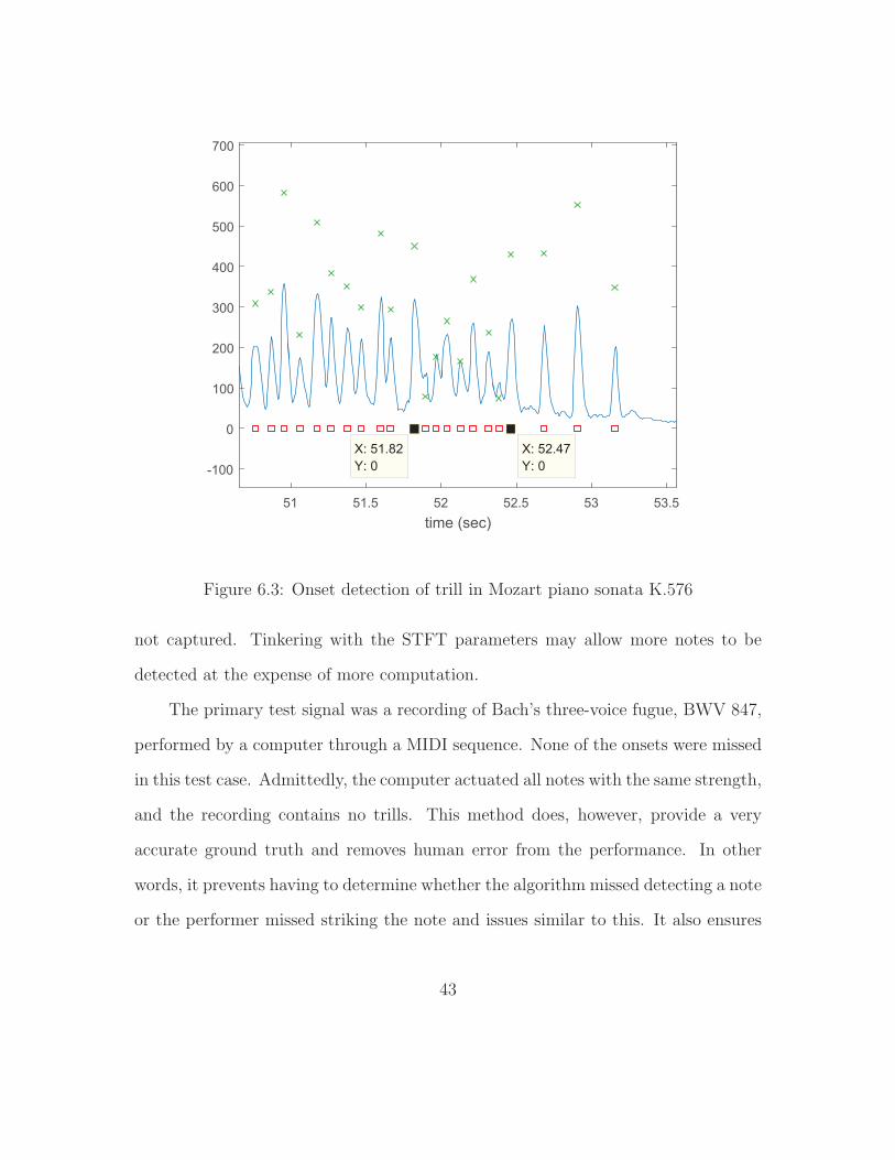
In the Mozart excerpt, it happens that all onsets are accurately detected. How-
ever, some musical excerpts do prove difficult, particularly tremolos and trills—
techniques involving rapid oscillation between notes. Figure 6.3 shows onset detec-
tion of a trill in the Allegro movement of Mozart’s K.576 sonata. The trill occurs
between the two marked onsets in the figure, and several onsets are missed. There
is a dramatic increase in the rate of notes at the beginning of the trill, but this is
40
1 2 3 4 5 6 7 8 9time (sec)
-50
-40
-30
-20
-10
0
10
20
30
40
50
Figure 6.1: Onset-finding intermediate of Mozart piano sonata K.545, measures 1-4
41
1 2 3 4 5 6 7 8 9time (sec)
0
50
100
150
200
250
300
350
400
Figure 6.2: Onset detection of Mozart piano sonata K.545, measures 1-4
42
51 51.5 52 52.5 53 53.5time (sec)
-100
0
100
200
300
400
500
600
700
X: 51.82Y: 0
X: 52.47Y: 0
Figure 6.3: Onset detection of trill in Mozart piano sonata K.576
not captured. Tinkering with the STFT parameters may allow more notes to be
detected at the expense of more computation.
The primary test signal was a recording of Bach’s three-voice fugue, BWV 847,
performed by a computer through a MIDI sequence. None of the onsets were missed
in this test case. Admittedly, the computer actuated all notes with the same strength,
and the recording contains no trills. This method does, however, provide a very
accurate ground truth and removes human error from the performance. In other
words, it prevents having to determine whether the algorithm missed detecting a note
or the performer missed striking the note and issues similar to this. It also ensures
43
highly accurate rhythmic execution. For these reasons, computer performance was
primarily considered.
6.2 Calibration Signal
The algorithm requires a calibration signal to create a dictionary of spectra—a
left and right spectrum for each note—which will be used to estimate the notes played
on that instrument in another recording. The signal is composed of the successive
individual playing of each note on the piano keyboard beginning with the lowest.
Onset detection is performed on this signal and the highest 88 onset scores are
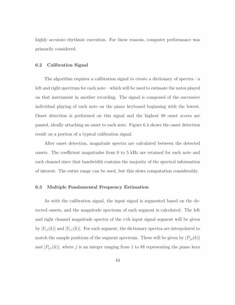
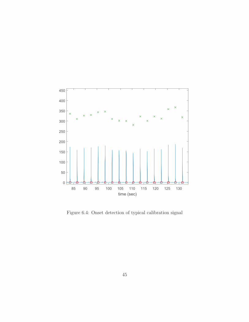
passed, ideally attaching an onset to each note. Figure 6.4 shows the onset detection
result on a portion of a typical calibration signal.
After onset detection, magnitude spectra are calculated between the detected
onsets. The coefficient magnitudes from 0 to 5 kHz are retained for each note and
each channel since that bandwidth contains the majority of the spectral information
of interest. The entire range can be used, but this slows computation considerably.
6.3 Multiple Fundamental Frequency Estimation
As with the calibration signal, the input signal is segmented based on the de-
tected onsets, and the magnitude spectrum of each segment is calculated. The left
and right channel magnitude spectra of the i-th input signal segment will be given
by |Yi,l(k)| and |Yi,r(k)|. For each segment, the dictionary spectra are interpolated to
match the sample positions of the segment spectrum. These will be given by |Pj,l(k)|and |Pj,r(k)|, where j is an integer ranging from 1 to 88 representing the piano keys
44
85 90 95 100 105 110 115 120 125 130time (sec)
0
50
100
150
200
250
300
350
400
450
Figure 6.4: Onset detection of typical calibration signal
45
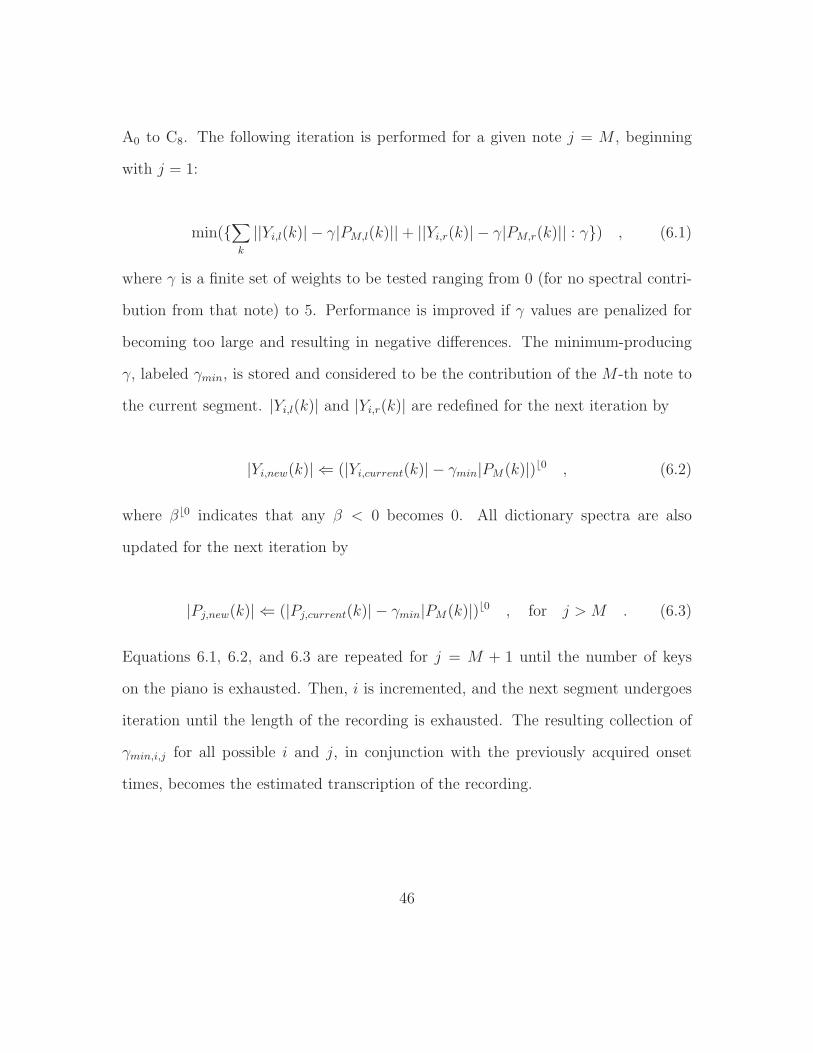
A0 to C8. The following iteration is performed for a given note j = M , beginning
with j = 1:
min({∑k
||Yi,l(k)| − γ|PM,l(k)||+ ||Yi,r(k)| − γ|PM,r(k)|| : γ}) , (6.1)
where γ is a finite set of weights to be tested ranging from 0 (for no spectral contri-
bution from that note) to 5. Performance is improved if γ values are penalized for
becoming too large and resulting in negative differences. The minimum-producing
γ, labeled γmin, is stored and considered to be the contribution of the M -th note to
the current segment. |Yi,l(k)| and |Yi,r(k)| are redefined for the next iteration by
|Yi,new(k)| ⇐ (|Yi,current(k)| − γmin|PM(k)|)�0 , (6.2)
where β�0 indicates that any β < 0 becomes 0. All dictionary spectra are also
updated for the next iteration by
|Pj,new(k)| ⇐ (|Pj,current(k)| − γmin|PM(k)|)�0 , for j > M . (6.3)
Equations 6.1, 6.2, and 6.3 are repeated for j = M + 1 until the number of keys
on the piano is exhausted. Then, i is incremented, and the next segment undergoes
iteration until the length of the recording is exhausted. The resulting collection of
γmin,i,j for all possible i and j, in conjunction with the previously acquired onset
times, becomes the estimated transcription of the recording.
46
6.4 Transcription Results
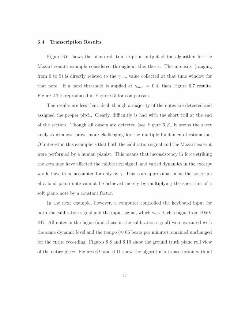
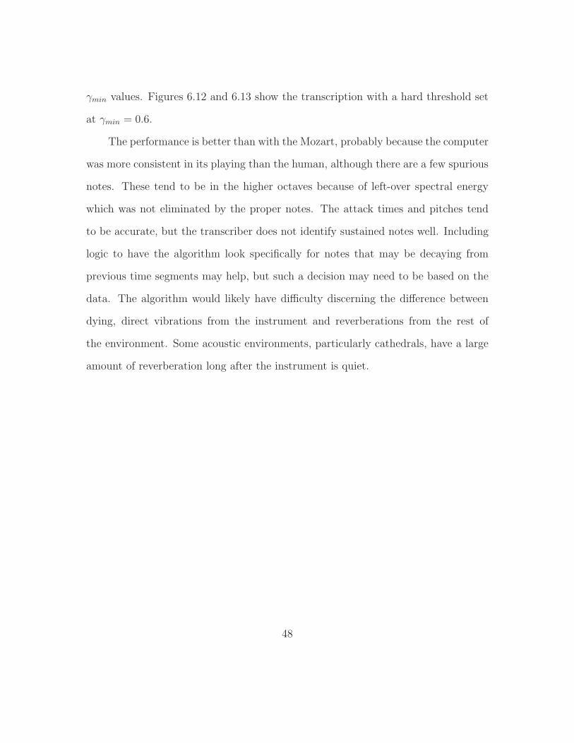
Figure 6.6 shows the piano roll transcription output of the algorithm for the
Mozart sonata example considered throughout this thesis. The intensity (ranging
from 0 to 5) is directly related to the γmin value collected at that time window for
that note. If a hard threshold is applied at γmin = 0.4, then Figure 6.7 results.
Figure 2.7 is reproduced in Figure 6.5 for comparison.
The results are less than ideal, though a majority of the notes are detected and
assigned the proper pitch. Clearly, difficultly is had with the short trill at the end
of the section. Though all onsets are detected (see Figure 6.2), it seems the short
analysis windows prove more challenging for the multiple fundamental estimation.
Of interest in this example is that both the calibration signal and the Mozart excerpt
were performed by a human pianist. This means that inconsistency in force striking
the keys may have affected the calibration signal, and varied dynamics in the excerpt
would have to be accounted for only by γ. This is an approximation as the spectrum
of a loud piano note cannot be achieved merely by multiplying the spectrum of a
soft piano note by a constant factor.
In the next example, however, a computer controlled the keyboard input for
both the calibration signal and the input signal, which was Bach’s fugue from BWV
847. All notes in the fugue (and those in the calibration signal) were executed with
the same dynamic level and the tempo (≈ 66 beats per minute) remained unchanged
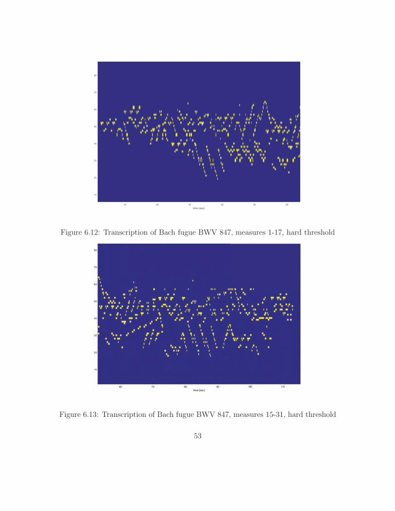
for the entire recording. Figures 6.8 and 6.10 show the ground truth piano roll view
of the entire piece. Figures 6.9 and 6.11 show the algorithm’s transcription with all
47
γmin values. Figures 6.12 and 6.13 show the transcription with a hard threshold set
at γmin = 0.6.
The performance is better than with the Mozart, probably because the computer
was more consistent in its playing than the human, although there are a few spurious
notes. These tend to be in the higher octaves because of left-over spectral energy
which was not eliminated by the proper notes. The attack times and pitches tend
to be accurate, but the transcriber does not identify sustained notes well. Including
logic to have the algorithm look specifically for notes that may be decaying from
previous time segments may help, but such a decision may need to be based on the
data. The algorithm would likely have difficulty discerning the difference between
dying, direct vibrations from the instrument and reverberations from the rest of
the environment. Some acoustic environments, particularly cathedrals, have a large
amount of reverberation long after the instrument is quiet.
48
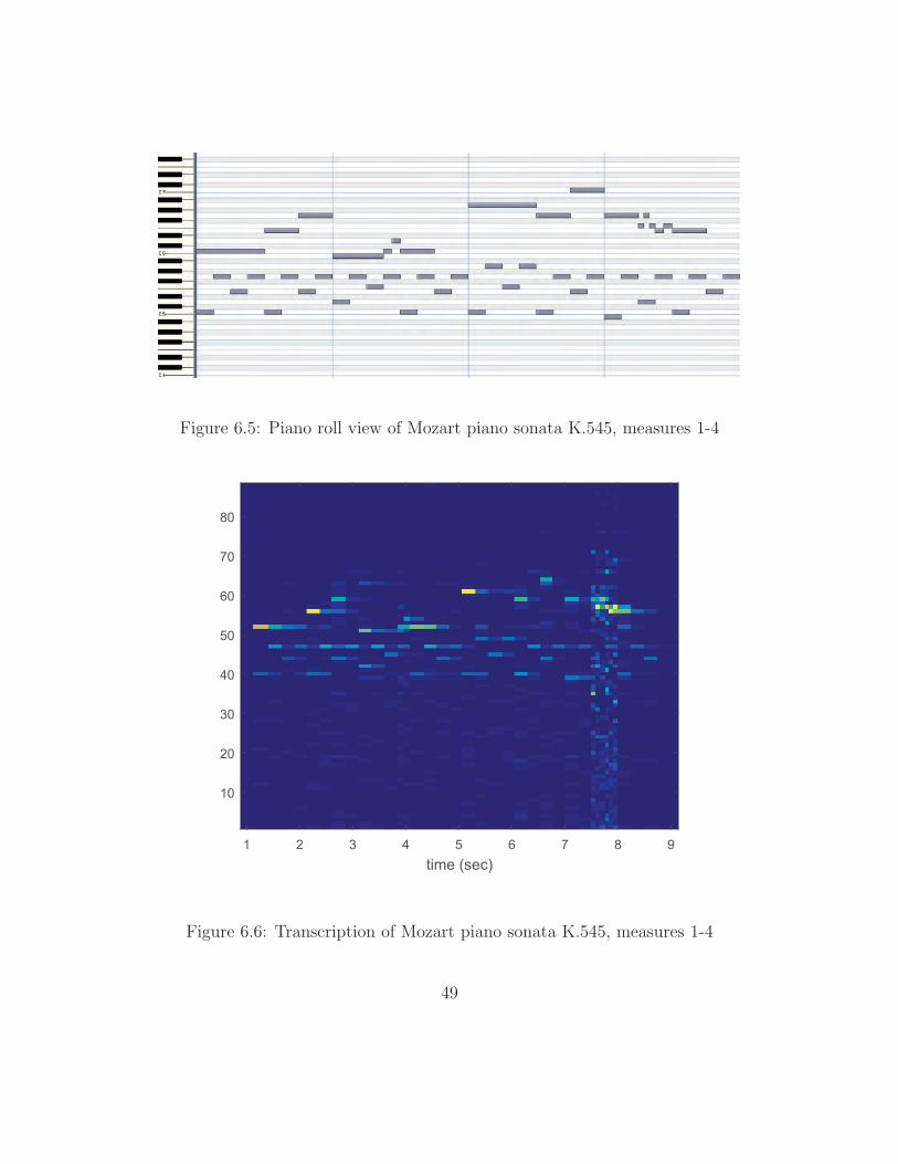
Figure 6.5: Piano roll view of Mozart piano sonata K.545, measures 1-4
1 2 3 4 5 6 7 8 9time (sec)
10
20
30
40
50
60
70
80
Figure 6.6: Transcription of Mozart piano sonata K.545, measures 1-4
49
1 2 3 4 5 6 7 8time (sec)
10
20
30
40
50
60
70
80
Figure 6.7: Transcription of Mozart piano sonata K.545, measures 1-4, hard threshold
50
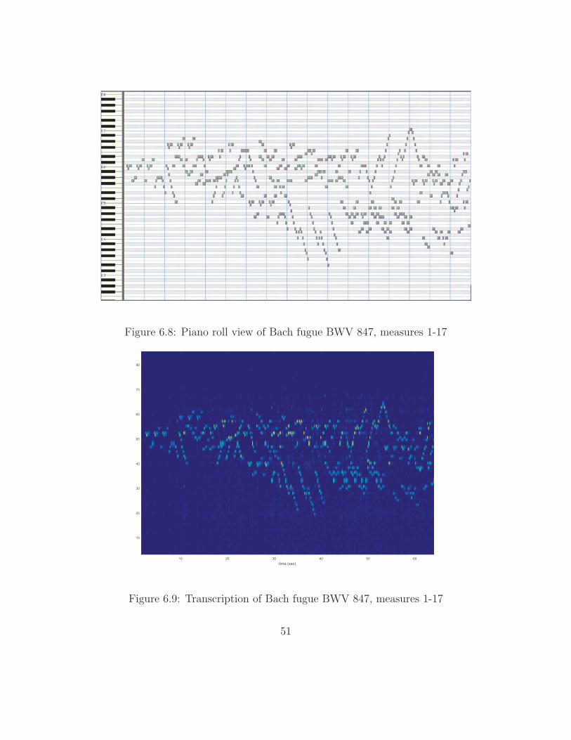
Figure 6.8: Piano roll view of Bach fugue BWV 847, measures 1-17
10 20 30 40 50 60time (sec)
10
20
30
40
50
60
70
80
Figure 6.9: Transcription of Bach fugue BWV 847, measures 1-17
51
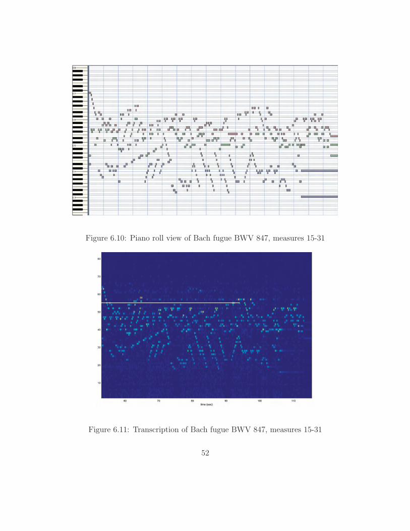
Figure 6.10: Piano roll view of Bach fugue BWV 847, measures 15-31
Figure 6.11: Transcription of Bach fugue BWV 847, measures 15-31
52
10 20 30 40 50 60time (sec)
10
20
30
40
50
60
70
80
Figure 6.12: Transcription of Bach fugue BWV 847, measures 1-17, hard threshold
Figure 6.13: Transcription of Bach fugue BWV 847, measures 15-31, hard threshold
53
Chapter 7
Conclusions and Future Work
An AMT algorithm has been described which works to transcribe piano record-
ings with reasonable accuracy, provided it has the benefit of a good calibration signal.
While the note onset detection system has seen prior use, this author is not aware
of previous use of the maximum frequency coefficient model for multiple fundamen-
tal frequency estimation. The AMT problem is a difficult one to solve, particularly
when operating in general, with little prior knowledge concerning the spectra of the
instruments involved.
In the future, perhaps the most obvious step is to attempt to remove the need
for a calibration signal. To achieve the same level of algorithm performance seen
here across various pianos without calibration would be a significant improvement.
Of course, there is always the interesting task of proceeding from the piano roll vi-
sualization to musical notation, though the subject did not receive much treatment
here. Expansion of the dataset would certainly lend insight into the algorithm per-
formance. Also, it is worth noting that this implementation is not strictly limited to
pianos. In theory, one could calibrate many different instruments or combinations
of instruments to function within the same framework. Adding multiple dictionary
entries for a single piano key, using varying dynamics, would likely improve perfor-
mance.
54
Bibliography
[1] The International Society of Music Information Retrieval. (2015). About theSociety [Online]. Available: www.ismir.net/society.html
[2] A. Klapuri and M. Davy, Eds., Signal Processing Methods for Music Transcrip-tion. New York: Springer, 2006.
[3] A. Spanias, T. Painter and V. Atti, Audio Signal Processing and Coding. Hobo-ken, NJ: John Wiley and Sons, Inc., 2007.
[4] N. Fletcher and T. Rossing, The Physics of Musical Instruments. 2nd ed. NewYork: Springer, 1998.
[5] H. Fletcher, “Normal Vibration Frequencies of a Stiff Piano String,” J. Acoust.Soc. Am., vol. 36, no. 1, pp. 203-209, Jan. 1964.
[6] N. Giordano, “Explaining the Railsback stretch in terms of the inharmonicityof piano tones and sensory dissonance,” J. Acoust. Soc. Am., vol. 138, no. 4, pp.2359-2366, Oct. 2015.
[7] N. Giordano, Physics of the Piano. New York: Oxford University Press, 2010.
[8] S. Mitra, Digital Signal Processing: A Computer-Based Approach. 4th ed. NewYork: McGraw-Hill, 2011.
[9] J. Smith, Spectral Audio Signal Processing. USA: W3K Publishing, 2011.
[10] D. Huber, The MIDI Manual: A Practical Guide to MIDI in the Project Studio.3rd ed. Burlington, MA: Focal Press, 2007.
[11] W. Mozart, “Sonate No. 15 fur das Pianoforte,” Wolfgang Amadeus MozartsWerke, Serie 20, no. 15, pp. 2-9 (174-181), Leipzig: Breitkopf & Hartel, 1878.
[12] J. Harnum, Basic Music Theory: How to Read, Write, and Understand WrittenMusic. 4th ed. Chicago: Sol Ut Press, 2013.
55
[13] S. Hainsworth and M. MacLeod, “Onset Detection in Musical Audio Signals,”Int. Comput. Music Conf., Singapore, 2003.
[14] A. Klapuri, A. Eronen and J. Astola, “Analysis of the Meter of Acoustic MusicalSignals,” IEEE Trans. Audio, Speech, and Lang. Process., vol. 14, no. 1, pp. 342-355, Jan. 2006.
[15] P. Masri and A. Bateman, “Improved Modelling of Attack Transients in Mu-sic Analysis-Resynthesis,” Int. Comput. Music Conf., pp. 100-103, Hong Kong,China, Aug. 1996.
[16] J. Bello, L. Daudet, S. Abdallah, et al., “A Tutorial on Onset Detection in MusicSignals,” IEEE Trans. Speech Audio Process., vol. 13, no. 5, Sept. 2005.
[17] B. Scherrer and P. Depalle, “Onset Time Estimation for the ExponentiallyDamped Sinusoids Analysis of Percussive Sounds,” Proc. 17th Int. Conf. DigitalAudio Effects, Erlangen, Germany, Sept. 2014.
[18] E. Benetos and S. Dixon, “Polyphonic Music Transcription Using Note Onsetand Offset Detection,” IEEE Int. Conf. Acoust., Speech and Signal Proc., pp.37-40, 2011.
[19] E. Benetos, S. Ewert and T. Weyde, “Automatic Transcription of Pitched andUnpitched Sounds from Polyphonic Music,” IEEE Int. Conf. Acoust., Speechand Signal Proc., pp. 3107-3111, 2014.
[20] S. Bock, A. Arzt, F. Krebs, et al., “Online Real-Time Onset Detection withRecurrent Neural Networks,” Proc. 15th Int. Conf. Digital Audio Effects, York,United Kingdom, Sept. 2012.
[21] G. Reis, F. Fernandez de Vega and A. Ferreira, “Automatic Transcription ofPolyphonic Piano Music Using Genetic Algorithms, Adaptive Spectral EnvelopeModeling, and Dynamic Noise Level Estimation,” IEEE Trans. Audio, Speech,and Lang. Proc., vol. 20, no. 8, Oct. 2012.
[22] A. Schutz and D. Slock, “Periodic Signal Modeling for the Octave Problem inMusic Transcription,” Int. Conf. on Digital Signal Proc., Santorini-Hellas, 2009.
[23] W. Szeto and K. Wong, “Source Separation and Analysis of Piano Music Sig-nals Using Instrument-Specific Sinusoidal Model,” Proc. 16th Int. Conf. DigitalAudio Effects, Maynooth, Ireland, Sept. 2013.
56
[24] A. Klapuri, “Multiple Fundamental Frequency Estimation by Summing Har-monic Amplitudes,” Proc. Int. Soc. Music Inform. Retrieval, Victoria, Canada,2006.
[25] C. Plack, A. Oxenham, R. Fay, et al., Eds., Pitch: Neural Coding and Perception.New York: Springer, 2005.
[26] A. Klapuri, “Signal Processing Methods for the Automatic Transcription ofMusic,” Ph.D. dissertation, Tampere Univ. of Tech., Tampere, Finland, 2004.
[27] E. Vincent, N. Bertin and R. Badeau, “Adaptive Harmonic Spectral Decompo-sition for Multiple Pitch Estimation,” IEEE Trans. Audio, Speech, and Lang.Proc., vol. 18, no. 3, Mar. 2010.
[28] C. Lee, Y. Yang and H. Chen, “Automatic Transcription of Piano Music bySparse Representation of Magnitude Spectra,” IEEE Int. Conf. Multimedia andExpo, Barcelona, Spain, Jul. 2011.
[29] N. Keriven, K. O’Hanlon and M. Plumbley, “Structured Sparsity Using Back-wards Elimination for Automatic Music Transcription,” IEEE Int. WorkshopMach. Learning for Signal Proc., Southampton, United Kingdom, Sept. 2013.
[30] A. Cogliati and Z. Duan, “Piano Music Transcription Modeling Note TemporalEvolution,” IEEE Int. Conf. Acoust., Speech and Signal Proc., pp. 429-433,South Brisbane, Queensland, Apr. 2015.
[31] V. Arora and L. Behera, “Multiple F0 Estimation and Source Clustering ofPolyphonic Music Audio Using PLCA and HMRFs,” IEEE/ACM Trans. Audio,Speech, and Lang. Proc., vol. 23, no. 2, Feb. 2015.
[32] K. O’Hanlon and M. Plumbley, “Polyphonic Piano Transcription Using Non-Negative Matrix Factorisation with Group Sparsity,” IEEE Int. Conf. Acoust.,Speech and Signal Proc., Florence, Italy, May 2014.
[33] L. Su and Y. Yang, “Combining Spectral and Temporal Representations forMultipitch Estimation of Polyphonic Music,” IEEE/ACM Trans. Audio, Speech,and Lang. Proc., vol. 23, no. 10, Oct. 2015.
[34] J. Bach and F. Kroll, Ed., “Prelude and Fugue in C minor, BWV 847,” Bach-Gesellschaft Ausgabe, Band 14, pp. 6-9, Leipzig: Breitkopf & Hartel, 1866.
57

Appendices
58
Appendix A
Bach BWV 847 Score
Following is the musical notation for the test signal using Bach’s three-voice
fugue, BWV 847. This edition is in the public domain and acquired from [34].
59