Embed Size (px)
Citation preview
Code_Aster Version v14
Titre : Notice d'utilisation du modèle THM Date : 25/11/2019 Page : 1/56Responsable : GRANET Sylvie Clé : U2.04.05 Révision :
6f5d72dfca70
Note of use of model THM
Summary:
Modelings THM exclusively treat evolution of the behaviors Thermo-Hydro-Mechanics of the saturated porousenvironments, or not, by one or two fluids. The digital and physical description as of these modelings inCode_Aster is detailed in [R7.01.10] and [R7.01.11].
One details in this documentation the procedure to be followed to carry out simulations in the context ofmodelings THM. One describes in the first part the various stages of calculations within the framework generalof continuous the mediums known as “generalized” (cf [R7.01.10]). In this part, one will not detail what relatesto the mechanical models described elsewhere. One restricts in the second part the application of thesemodelings to treat the porous environments which undergo a degradation of their mechanical properties perdamage of the ground or the rocks for example. For that, one extends modelings THM to the mediumswith microstructure by taking of account the effects second gradient (cf [R5.04.03]). The objective is to correctthe dependence with the space discretization of the solutions when the mechanical law of behavior consideredis of lenitive type – what is the case for any fragile material, and thus the grounds in particular.
Warning : The translation process used on this website is a "Machine Translation". It may be imprecise and inaccurate in whole or in part and isprovided as a convenience.Copyright 2021 EDF R&D - Licensed under the terms of the GNU FDL (http://www.gnu.org/copyleft/fdl.html)
Code_Aster Version v14
Titre : Notice d'utilisation du modèle THM Date : 25/11/2019 Page : 2/56Responsable : GRANET Sylvie Clé : U2.04.05 Révision :
6f5d72dfca70
Contents1 Broad outlines ....................................................................................................................................... 4
1.1 Context of studies THM ................................................................................................................. 4
1.2 General information ....................................................................................................................... 4
1.3 Stages of calculations .................................................................................................................... 5
2 Various stages of a calculation THM .................................................................................................... 5
2.1 Choice of the model ....................................................................................................................... 5
2.2 Definition of material ...................................................................................................................... 9
2.2.1 Simple keyword COMP_THM ............................................................................................. 10
2.2.2 Keyword factor THM_INIT .................................................................................................. 12
2.2.3 Keyword factor THM_LIQU ................................................................................................. 14
2.2.4 Keyword factor THM_GAZ .................................................................................................. 15
2.2.5 Keyword factor THM_VAPE_GAZ ...................................................................................... 16
2.2.6 Keyword factor THM_AIR_DISS ......................................................................................... 16
2.2.7 Keyword factor THM_DIFFU ............................................................................................... 17
2.2.8 Summary of the functions of couplings and their dependence ........................................... 24
Keyword factor THM_DIFFU ............................................................................................. 25
2.3 Initialization of calculation ............................................................................................................ 28
2.4 Loadings and boundary conditions ............................................................................................... 30
2.5 Nonlinear calculation .................................................................................................................... 33
2.5.1 Resolution by coupling ........................................................................................................ 33
2.5.2 Resolution by chaining ........................................................................................................ 34
2.5.3 General advices of use ....................................................................................................... 36
2.6 Postprocessing ............................................................................................................................. 41
2.6.1 General information ............................................................................................................ 41
2.6.2 Internal variables ................................................................................................................ 42
2.6.3 Isovaleurs ........................................................................................................................... 44
2.7 Some cases tests ......................................................................................................................... 45
3 Modelings THM by an approach second gradient ............................................................................... 46
3.1 Definition of the patch .................................................................................................................. 46
3.1.1 Stage 1. Definition of the grid of the structure .................................................................... 47
3.1.2 Stage 2. Duplication of the grid to define the patch ............................................................ 47
3.1.3 Stage 3. Modification (possible) of the grid of the patch .................................................... 47
3.2 Choice of the model ..................................................................................................................... 47
3.3 Definition of material .................................................................................................................... 48
3.4 Impact on the boundary conditions .............................................................................................. 49
3.5 Resolution DU problem ................................................................................................................ 49
Annexe 1 Generalized constraints and internal variables ..................................................................... 50
Annexe 2 Additional elements on the boundary conditions in THM ....................................................... 52
Warning : The translation process used on this website is a "Machine Translation". It may be imprecise and inaccurate in whole or in part and isprovided as a convenience.Copyright 2021 EDF R&D - Licensed under the terms of the GNU FDL (http://www.gnu.org/copyleft/fdl.html)
Code_Aster Version v14
Titre : Notice d'utilisation du modèle THM Date : 25/11/2019 Page : 3/56Responsable : GRANET Sylvie Clé : U2.04.05 Révision :
6f5d72dfca70
Warning : The translation process used on this website is a "Machine Translation". It may be imprecise and inaccurate in whole or in part and isprovided as a convenience.Copyright 2021 EDF R&D - Licensed under the terms of the GNU FDL (http://www.gnu.org/copyleft/fdl.html)
Code_Aster Version v14
Titre : Notice d'utilisation du modèle THM Date : 25/11/2019 Page : 4/56Responsable : GRANET Sylvie Clé : U2.04.05 Révision :
6f5d72dfca70
1 Broad outlines
1.1 Context of studies THMFirst of all, it is advisable to define the quite precise framework of calculations Thermo-Hydro-Mechanics. Those have as an exclusive application the study of the porous environments. Knowingthat, modeling THM covers the mechanical evolution of these mediums and the flows in their centre.The latter relate to one or two fluids and are governed by the laws of Darcy (fluid darcéens). Theproblem of complete THM thus treats flow of or fluid (S), mechanics of the skeleton, as well asthermics: the resolution is very often entirely coupled. It can also be chained whenever thephenomena hydraulics and mechanics are slightly coupled.
Note:
In the expression of the laws of Darcy which is retained here, one neglects the differentialacceleration of water. In the case of very permeable and very porous mediums subjected toa seismic loading, that can constitute a limit.
1.2 General informationCalculations are based on families of laws of behavior THM for the saturated and unsaturated porousenvironments. The mechanics of the porous environments gathers a very exhaustive collection ofphysical phenomena concerning to the solids and the fluids. It makes the assumption of a couplingbetween the mechanical evolutions of the solids and the fluids, seen like continuous mediums, withthe hydraulic evolutions, which solve the problems of diffusion of fluids within walls or volumes, andthe thermal evolutions. The formulation of modeling Thermo-hydro-mechanics (THM) in porousenvironment such as it is made in Code_Aster is detailed in [R7.01.11] and [R7.01.10]. All thenotations employed here thus refer to it. One points out some essential notations however thereafter:
Concerning the fluids, one considers (the most complete case) two phases (liquid and gas) and twocomponents called by convenience water and air. The following indices then are used:
w for liquid waterad for the dissolved air
as for the dry airvp for the steam
The thermodynamic variables are: • pressures of the components: pw x , t , pad x ,t , pvp x ,t , pas x , t ,
• the temperature of the medium T x , t .
These various variables are not completely independent. Indeed, if only one component is considered,thermodynamic balance between its phases imposes a relation between the steam pressure and thepressure of the liquid of this component. Finally, there is only one independent pressure percomponent, just as there is only one conservation equation of the mass. The number of independentpressures is thus equal to the number of independent components. The choice of these pressuresvaries according to the laws of behaviors.
For the case known as saturated (only one component air or water), we chose the pressure of thissingle constituting.For the case says unsaturated (presence of air and water), we chose like independent variables:
• total pressure of gas p gz x ,t = pvp pas ,
• capillary pressure pc x , t = pgz− plq= pgz−pw− pad .
We will see thereafter the terminology Aster for these variables.
Warning : The translation process used on this website is a "Machine Translation". It may be imprecise and inaccurate in whole or in part and isprovided as a convenience.Copyright 2021 EDF R&D - Licensed under the terms of the GNU FDL (http://www.gnu.org/copyleft/fdl.html)
Code_Aster Version v14
Titre : Notice d'utilisation du modèle THM Date : 25/11/2019 Page : 5/56Responsable : GRANET Sylvie Clé : U2.04.05 Révision :
6f5d72dfca70
1.3 Stages of calculations
For the stages necessary to the implementation of a calculation Aster, independently of aspectspurely THM, one will refer to the documentation of each order used.
In any calculation Aster, several key stages must be carried out:
• Choice of modeling• Data materials• Initialization• Calculation• Postprocessing
These points are detailed in the following chapter.
2 Various stages of a calculation THM
2.1 Choice of the model
The digital processing in THM requires a quadratic grid since the elements are of type P2 indisplacement and P1 in pressure and temperature in order to avoid problems of oscillations.
The choice is done by the use of the order AFFE_MODELE as in example Ci - below:
MODELE=AFFE_MODELE (MAILLAGE=MAIL, AFFE=_F (TOUT=' OUI', PHENOMENE=' MECANIQUE', MODELISATION=' AXIS_THH2MD',),)
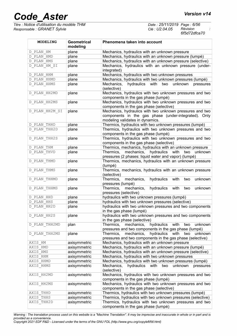
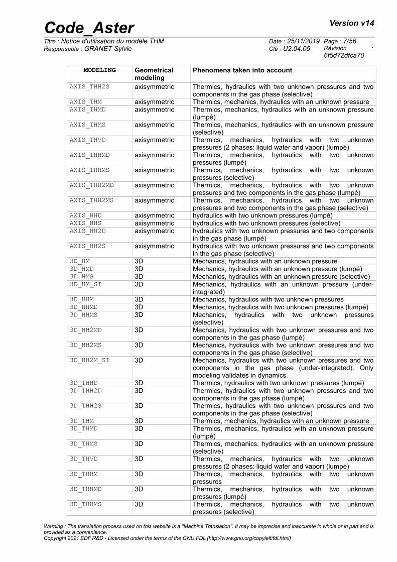
In all the cases, the phenomenon is ‘MECHANICAL’ (even if modeling does not contain mechanics).The user must then inform in an obligatory way the keyword MODELING. This keyword makes itpossible to define the type of affected element in a kind of mesh. Modelings available in THM areindicated in the table 2.1-1.
Notice concerning the digital processing (keyword ending in D or S):
Modelings ending in the letter D indicate that one makes a treatment allowing of diagonaliser(“lumper”) the matrix in order to avoid the oscillations for the hydraulic problems. For that the points ofintegration are taken at the tops of the elements. This treatment being adapted little to mechanics, onealso has a modeling known as “selective”. In this case, the capacitive terms are integrated into thetops whereas the diffusive terms are integrated into the points of Gauss. These modelings end in S.other modelings integrate all into the point of Gauss.
One highly advises with the user to use modelings D or S in the cases without mechanics and to usemodeling S and for modelings with mechanics.
“Classical” modelings (without D nor S) are brought to be reabsorbed and are disadvised.
Warning : The translation process used on this website is a "Machine Translation". It may be imprecise and inaccurate in whole or in part and isprovided as a convenience.Copyright 2021 EDF R&D - Licensed under the terms of the GNU FDL (http://www.gnu.org/copyleft/fdl.html)
Code_Aster Version v14
Titre : Notice d'utilisation du modèle THM Date : 25/11/2019 Page : 6/56Responsable : GRANET Sylvie Clé : U2.04.05 Révision :
6f5d72dfca70
MODELING Geometricalmodeling
Phenomena taken into account
D_PLAN_HM plane Mechanics, hydraulics with an unknown pressureD_PLAN_HMD plane Mechanics, hydraulics with an unknown pressure (lumpé)D_PLAN_HMS plane Mechanics, hydraulics with an unknown pressure (selective)D_PLAN_HM_SI plane Mechanics, hydraulics with an unknown pressure (under-
integrated)D_PLAN_HHM plane Mechanics, hydraulics with two unknown pressuresD_PLAN_HHMD plane Mechanics, hydraulics with two unknown pressures (lumpé)D_PLAN_HHMS plane Mechanics, hydraulics with two unknown pressures
(selective)D_PLAN_HH2MD plane Mechanics, hydraulics with two unknown pressures and two
components in the gas phase (lumpé)D_PLAN_HH2MS plane Mechanics, hydraulics with two unknown pressures and two
components in the gas phase (selective)D_PLAN_HH2M_SI plane Mechanics, hydraulics with two unknown pressures and two
components in the gas phase (under-integrated). Onlymodeling validates in dynamics.
D_PLAN_THHD plane Thermics, hydraulics with two unknown pressures (lumpé)D_PLAN_THH2D plane Thermics, hydraulics with two unknown pressures and two
components in the gas phase (lumpé)D_PLAN_THH2S plane Thermics, hydraulics with two unknown pressures and two
components in the gas phase (selective)D_PLAN_THM plane Thermics, mechanics, hydraulics with an unknown pressureD_PLAN_THVD plane Thermics, mechanics, hydraulics with two unknown
pressures (2 phases: liquid water and vapor) (lumpé)D_PLAN_THMD plane Thermics, mechanics, hydraulics with an unknown pressure
(lumpé)D_PLAN_THMS plane Thermics, mechanics, hydraulics with an unknown pressure
(selective)D_PLAN_THHMD plane Thermics, mechanics, hydraulics with two unknown
pressures (lumpé)D_PLAN_THHMS plane Thermics, mechanics, hydraulics with two unknown
pressures (selective)D_PLAN_HHD plane hydraulics with two unknown pressures (lumpé)D_PLAN_HHS plane hydraulics with two unknown pressures (selective)D_PLAN_HH2D plane hydraulics with two unknown pressures and two components
in the gas phase (lumpé)D_PLAN_HH2S plane hydraulics with two unknown pressures and two components
in the gas phase (selective)D_PLAN_THH2MD plan Thermics, mechanics, hydraulics with two unknown
pressures and two components in the gas phase (lumpé)D_PLAN_THH2MS plane Thermics, mechanics, hydraulics with two unknown
pressures and two components in the gas phase (selective)AXIS_HM axisymmetric Mechanics, hydraulics with an unknown pressureAXIS_HMD axisymmetric Mechanics, hydraulics with an unknown pressure (lumpé)AXIS_HMS axisymmetric Mechanics, hydraulics with an unknown pressure (selective)AXIS_HHM axisymmetric Mechanics, hydraulics with two unknown pressuresAXIS_HHMD axisymmetric Mechanics, hydraulics with two unknown pressures (lumpé)AXIS_HHMS axisymmetric Mechanics, hydraulics with two unknown pressures
(selective)AXIS_HH2MD axisymmetric Mechanics, hydraulics with two unknown pressures and two
components in the gas phase (lumpé)AXIS_HH2MS axisymmetric Mechanics, hydraulics with two unknown pressures and two
components in the gas phase (selective)AXIS_THHD axisymmetric Thermics, hydraulics with two unknown pressures (lumpé)AXIS_THHS axisymmetric Thermics, hydraulics with two unknown pressures (selective)AXIS_THH2D axisymmetric Thermics, hydraulics with two unknown pressures and two
components in the gas phase (lumpé)
Warning : The translation process used on this website is a "Machine Translation". It may be imprecise and inaccurate in whole or in part and isprovided as a convenience.Copyright 2021 EDF R&D - Licensed under the terms of the GNU FDL (http://www.gnu.org/copyleft/fdl.html)
Code_Aster Version v14
Titre : Notice d'utilisation du modèle THM Date : 25/11/2019 Page : 7/56Responsable : GRANET Sylvie Clé : U2.04.05 Révision :
6f5d72dfca70
MODELING Geometricalmodeling
Phenomena taken into account
AXIS_THH2S axisymmetric Thermics, hydraulics with two unknown pressures and twocomponents in the gas phase (selective)
AXIS_THM axisymmetric Thermics, mechanics, hydraulics with an unknown pressureAXIS_THMD axisymmetric Thermics, mechanics, hydraulics with an unknown pressure
(lumpé)AXIS_THMS axisymmetric Thermics, mechanics, hydraulics with an unknown pressure
(selective)AXIS_THVD axisymmetric Thermics, mechanics, hydraulics with two unknown
pressures (2 phases: liquid water and vapor) (lumpé)AXIS_THHMD axisymmetric Thermics, mechanics, hydraulics with two unknown
pressures (lumpé)AXIS_THHMS axisymmetric Thermics, mechanics, hydraulics with two unknown
pressures (selective)AXIS_THH2MD axisymmetric Thermics, mechanics, hydraulics with two unknown
pressures and two components in the gas phase (lumpé)AXIS_THH2MS axisymmetric Thermics, mechanics, hydraulics with two unknown
pressures and two components in the gas phase (selective)AXIS_HHD axisymmetric hydraulics with two unknown pressures (lumpé)AXIS_HHS axisymmetric hydraulics with two unknown pressures (selective)AXIS_HH2D axisymmetric hydraulics with two unknown pressures and two components
in the gas phase (lumpé)AXIS_HH2S axisymmetric hydraulics with two unknown pressures and two components
in the gas phase (selective)3D_HM 3D Mechanics, hydraulics with an unknown pressure3D_HMD 3D Mechanics, hydraulics with an unknown pressure (lumpé)3D_HMS 3D Mechanics, hydraulics with an unknown pressure (selective)3D_HM_SI 3D Mechanics, hydraulics with an unknown pressure (under-
integrated)3D_HHM 3D Mechanics, hydraulics with two unknown pressures3D_HHMD 3D Mechanics, hydraulics with two unknown pressures (lumpé)3D_HHMS 3D Mechanics, hydraulics with two unknown pressures
(selective)3D_HH2MD 3D Mechanics, hydraulics with two unknown pressures and two
components in the gas phase (lumpé)3D_HH2MS 3D Mechanics, hydraulics with two unknown pressures and two
components in the gas phase (selective)3D_HH2M_SI 3D Mechanics, hydraulics with two unknown pressures and two
components in the gas phase (under-integrated). Onlymodeling validates in dynamics.
3D_THHD 3D Thermics, hydraulics with two unknown pressures (lumpé)3D_THH2D 3D Thermics, hydraulics with two unknown pressures and two
components in the gas phase (lumpé)3D_THH2S 3D Thermics, hydraulics with two unknown pressures and two
components in the gas phase (selective)3D_THM 3D Thermics, mechanics, hydraulics with an unknown pressure3D_THMD 3D Thermics, mechanics, hydraulics with an unknown pressure
(lumpé)3D_THMS 3D Thermics, mechanics, hydraulics with an unknown pressure
(selective)3D_THVD 3D Thermics, mechanics, hydraulics with two unknown
pressures (2 phases: liquid water and vapor) (lumpé)3D_THHM 3D Thermics, mechanics, hydraulics with two unknown
pressures3D_THHMD 3D Thermics, mechanics, hydraulics with two unknown
pressures (lumpé)3D_THHMS 3D Thermics, mechanics, hydraulics with two unknown
pressures (selective)
Warning : The translation process used on this website is a "Machine Translation". It may be imprecise and inaccurate in whole or in part and isprovided as a convenience.Copyright 2021 EDF R&D - Licensed under the terms of the GNU FDL (http://www.gnu.org/copyleft/fdl.html)
Code_Aster Version v14
Titre : Notice d'utilisation du modèle THM Date : 25/11/2019 Page : 8/56Responsable : GRANET Sylvie Clé : U2.04.05 Révision :
6f5d72dfca70
MODELING Geometricalmodeling
Phenomena taken into account
3D_THH2MD 3D Thermics, mechanics, hydraulics with two unknownpressures and two components in the gas phase (lumpé)
3D_THH2MS 3D Thermics, mechanics, hydraulics with two unknownpressures and two components in the gas phase (selective)
3D_HHD 3D hydraulics with two unknown pressures (lumpé)3D_HHS 3D hydraulics with two unknown pressures (selective)3D_HH2D 3D hydraulics with two unknown pressures and two components
in the gas phase (lumpé)3D_HH2S 3D hydraulics with two unknown pressures and two components
in the gas phase (selective)
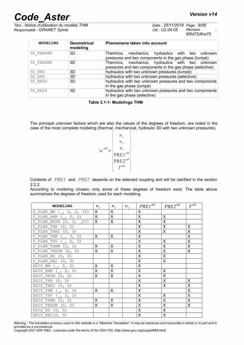
Table 2.1-1: Modelings THM
The principal unknown factors which are also the values of the degrees of freedom, are noted in thecase of the most complete modeling (thermal, mechanical, hydraulic 3D with two unknown pressures).
{u }ddl={
ux
u y
uz
PRE1ddl
PRE2ddl
T ddl}
Contents of PRE1 and PRE2 depends on the selected coupling and will be clarified in the section2.2.2. According to modeling chosen, only some of these degrees of freedom exist. The table abovesummarizes the degrees of freedom used for each modeling.
MODELING ux u y uz PRE1ddl PRE2ddl T ddl D_PLAN_HM (_, S, D, IF) X X XD_PLAN_HHM (_, S, D) X X X XD_PLAN_HH2M (S, D, _SI) X X X XD_PLAN_THH (S, D) X X XD_PLAN_THH2 (S, D) X X XD_PLAN_THM (_, S, D) X X X XD_PLAN_THV (_, S, D) X X XD_PLAN_THHM (S, D) X X X X XD_PLAN_THH2M (S, D) X X X X XD_PLAN_HH (S, D) X XD_PLAN_HH2 (S, D) X XAXIS_HM (_, S, D) X X XAXIS_HHM (_, S, D) X X X XAXIS_HH2M (S, D) X X X XAXIS_THH (S, D) X X XAXIS_THH2 (S, D) X X XAXIS_THM (_, S, D) X X X XAXIS_THV (_, S, D) X X XAXIS_THHM (S, D) X X X X XAXIS_THH2M (S, D) X X X X XAXIS_HH (S, D) X XAXIS_HH2(S, D) X X
Warning : The translation process used on this website is a "Machine Translation". It may be imprecise and inaccurate in whole or in part and isprovided as a convenience.Copyright 2021 EDF R&D - Licensed under the terms of the GNU FDL (http://www.gnu.org/copyleft/fdl.html)
Code_Aster Version v14
Titre : Notice d'utilisation du modèle THM Date : 25/11/2019 Page : 9/56Responsable : GRANET Sylvie Clé : U2.04.05 Révision :
6f5d72dfca70
MODELING ux u y uz PRE1ddl PRE2ddl T ddl 3D_HM(_, S, D, IF) X X X X3D_HHM(_, S, D) X X X X X3D_HH2M(S, D, _SI) X X X X X3D_THH (S, D) X X X3D_THH2D X X X3D_THM (_, S, D) X X X X X3D_THVD (_, S, D) X X X3D_THHM(_, S, D) X X X X X X3D_THH2M (S, D) X X X X X X3D_HH(S, D) X X3D_HH2 (S, D) X X
The generalized constraints and the internal variables all are indicated in [§Annexe 1]. The notationsused are those defined in [R7.01.11].
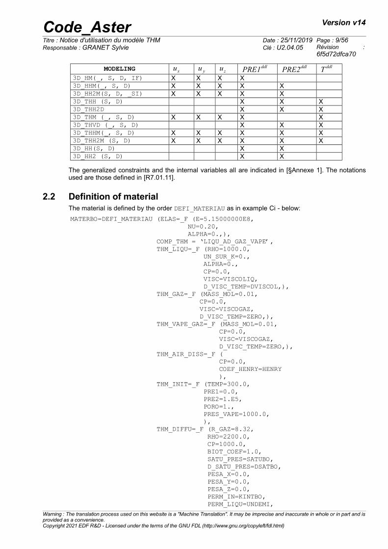
2.2 Definition of materialThe material is defined by the order DEFI_MATERIAU as in example Ci - below:
MATERBO=DEFI_MATERIAU (ELAS=_F (E=5.15000000E8, NU=0.20, ALPHA=0.,), COMP_THM = ‘LIQU_AD_GAZ_VAPE’, THM_LIQU=_F (RHO=1000.0, UN_SUR_K=0., ALPHA=0., CP=0.0, VISC=VISCOLIQ, D_VISC_TEMP=DVISCOL,), THM_GAZ=_F (MASS_MOL=0.01, CP=0.0, VISC=VISCOGAZ, D_VISC_TEMP=ZERO,), THM_VAPE_GAZ=_F (MASS_MOL=0.01, CP=0.0, VISC=VISCOGAZ, D_VISC_TEMP=ZERO,), THM_AIR_DISS=_F ( CP=0.0, COEF_HENRY=HENRY ), THM_INIT=_F (TEMP=300.0, PRE1=0.0, PRE2=1.E5, PORO=1., PRES_VAPE=1000.0, ), THM_DIFFU=_F (R_GAZ=8.32, RHO=2200.0, CP=1000.0, BIOT_COEF=1.0, SATU_PRES=SATUBO, D_SATU_PRES=DSATBO, PESA_X=0.0, PESA_Y=0.0, PESA_Z=0.0, PERM_IN=KINTBO, PERM_LIQU=UNDEMI,
Warning : The translation process used on this website is a "Machine Translation". It may be imprecise and inaccurate in whole or in part and isprovided as a convenience.Copyright 2021 EDF R&D - Licensed under the terms of the GNU FDL (http://www.gnu.org/copyleft/fdl.html)
Code_Aster Version v14
Titre : Notice d'utilisation du modèle THM Date : 25/11/2019 Page : 10/56Responsable : GRANET Sylvie Clé : U2.04.05 Révision :
6f5d72dfca70
D_PERM_LIQU_SATU=ZERO, PERM_GAZ=UNDEMI, D_PERM_SATU_GAZ=ZERO, D_PERM_PRES_GAZ=ZERO, FICKV_T=ZERO, FICKA_T=FICK, LAMB_T=ZERO, ),); We now will detail each keywords. We will not stick here to the mechanical part – so mechanical thereis - which depends on the selected law of behavior. One will refer for that to the documentation ofDEFI_MATERIAU (U4.43.01).
2.2.1 Simple keyword COMP_THM
Allows to select as of the definition of material the mixing rate THM. The possible laws are
♦ COMP_THM = / ‘LIQU_SATU ‘ , / ‘LIQU_GAZ ‘ , / ‘GAS ‘ , / ‘LIQU_GAZ_ATM ‘ , / ‘LIQU_AD_GAZ ‘ , / ‘LIQU_VAPE_GAZ ‘, / ‘LIQU_AD_GAZ_VAPE ‘, / ‘LIQU_VAPE ‘ ,/ ‘GAS’
Law of reaction of a perfect gas i.e. checking the relation P /=RT /Mv where P is the
pressure, density, Mv molar mass, R the constant of perfect gases and T the temperature(confer [R7.01.11] for more details). For an only saturated medium. The data necessary of thefield material are provided in the operator DEFI_MATERIAU, under the keyword THM_GAZ.
/ ‘LIQU_SATU’
Law of behavior for porous environments saturated by only one liquid (cf [R7.01.11] for moredetails). The data necessary of the field material are provided in the operator DEFI_MATERIAU,under the keyword THM_LIQU.
/ ‘LIQU_GAZ_ATM’
Law of behavior for a porous environment unsaturated with a liquid and gas with atmosphericpressure (confer [R7.01.11] for more details). The data necessary of the field material areprovided in the operator DEFI_MATERIAU, under the keywords THM_LIQU and THM_GAZ.
/ ‘LIQU_VAPE_GAZ’
Law of behavior for a porous environment unsaturated water/vapor/dry air with phase shift (confer[R7.01.11] for more details). The data necessary of the field material are provided in the operatorDEFI_MATERIAU, under the keywords THM_LIQU, THM_VAPE and THM_GAZ.
/ ‘LIQU_AD_GAZ_VAPE’
Law of behavior for a porous environment unsaturated water/vapor/dry air/air dissolved withphase shift (confer [R7.01.11] for more details). The data necessary of the field material areprovided in the operator DEFI_MATERIAU, under the keywords THM_LIQU, THM_VAPE, THM_GAZand THM_AIR_DISS.
/ ‘LIQU_AD_GAZ’
Law of behavior for a porous environment unsaturated water/dry air/air dissolved with phase shift(confer [R7.01.11] for more details). The data necessary of the field material are provided in theoperator DEFI_MATERIAU, under the keywords THM_LIQU, THM_GAZ and THM_AIR_DISS.
Warning : The translation process used on this website is a "Machine Translation". It may be imprecise and inaccurate in whole or in part and isprovided as a convenience.Copyright 2021 EDF R&D - Licensed under the terms of the GNU FDL (http://www.gnu.org/copyleft/fdl.html)
Code_Aster Version v14
Titre : Notice d'utilisation du modèle THM Date : 25/11/2019 Page : 11/56Responsable : GRANET Sylvie Clé : U2.04.05 Révision :
6f5d72dfca70
/ ‘LIQU_VAPE’
Law of behavior for porous environments saturated by a component present in liquid form orvapor with phase shift (confer [R7.01.11] for more details). The data necessary of the fieldmaterial are provided in the operator DEFI_MATERIAU, under the keywords THM_LIQU andTHM_VAPE. This law is valid only for modelings of the type THVD.
/ ‘LIQU_GAZ’
Law of behavior for a porous environment unsaturated liquid/gas without phase shift (confer[R7.01.11] for more details). The data necessary of the field material are provided in the operatorDEFI_MATERIAU, under the keywords THM_LIQU and THM_GAZ.
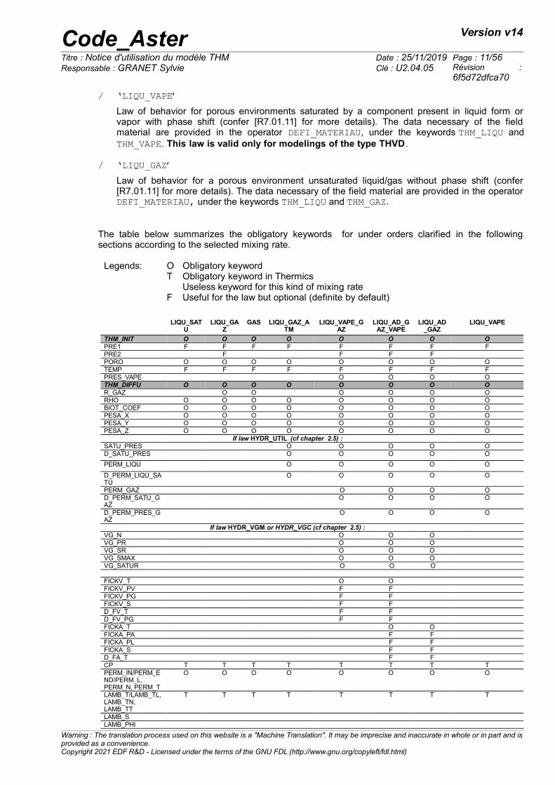
The table below summarizes the obligatory keywords for under orders clarified in the followingsections according to the selected mixing rate.
Legends: O Obligatory keywordT Obligatory keyword in Thermics
Useless keyword for this kind of mixing rateF Useful for the law but optional (definite by default)
LIQU_SATU
LIQU_GAZ
GAS LIQU_GAZ_ATM
LIQU_VAPE_GAZ
LIQU_AD_GAZ_VAPE
LIQU_AD_GAZ
LIQU_VAPE
THM_INIT O O O O O O O OPRE1 F F F F F F F FPRE2 F F F F PORO O O O O O O O OTEMP F F F F F F F FPRES_VAPE O O O OTHM_DIFFU O O O O O O O OR_GAZ O O O O O ORHO O O O O O O O OBIOT_COEF O O O O O O O OPESA_X O O O O O O O OPESA_Y O O O O O O O OPESA_Z O O O O O O O O
If law HYDR_UTIL (cf chapter 2.5) :SATU_PRES O O O O OD_SATU_PRES O O O O O
PERM_LIQU O O O O O
D_PERM_LIQU_SATU
O O O O O
PERM_GAZ O O O OD_PERM_SATU_GAZ
O O O O
D_PERM_PRES_GAZ
O O O O
If law HYDR_VGM or HYDR_VGC (cf chapter 2.5) :VG_N O O OVG_PR O O OVG_SR O O OVG_SMAX O O OVG_SATUR O O O
FICKV_T O O FICKV_PV F FFICKV_PG F FFICKV_S F FD_FV_T F FD_FV_PG F F FICKA_T O OFICKA_PA F FFICKA_PL F FFICKA_S F FD_FA_T F FCP T T T T T T T TPERM_IN/PERM_END/PERM_L,PERM_N, PERM_T
O O O O O O O O
LAMB_T/LAMB_TL,LAMB_TN,LAMB_TT
T T T T T T T T
LAMB_SLAMB_PHI
Warning : The translation process used on this website is a "Machine Translation". It may be imprecise and inaccurate in whole or in part and isprovided as a convenience.Copyright 2021 EDF R&D - Licensed under the terms of the GNU FDL (http://www.gnu.org/copyleft/fdl.html)
Code_Aster Version v14
Titre : Notice d'utilisation du modèle THM Date : 25/11/2019 Page : 12/56Responsable : GRANET Sylvie Clé : U2.04.05 Révision :
6f5d72dfca70
LAMB_CT/LAMB_C_L, LAMB_C_N,LAMB_C_TD_LB_T/D_LB_TOUT, D_LB_TL,D_LB_T,D_LB_SD_LB_PHITHM_LIQU O O O O O O ORHO O O O O O O OUN_SUR_K O O O O O O OVISC O O O O O O OD_VISC_TEMP O O O O O O OALPHA T T T T T T TCP T T T T T T TTHM_GAZ O O O O O OMASS_MOL O O O O O OVISC O O O O O OD_VISC_TEMP O O O O O OCP T T T T T TTHM_VAPE_GAZ O O OMASS_MOL O O OCP O O OVISC O O OD_VISC_TEMP O O OTHM_AIR_DISS O OCP O OCOEF_HENRY O O
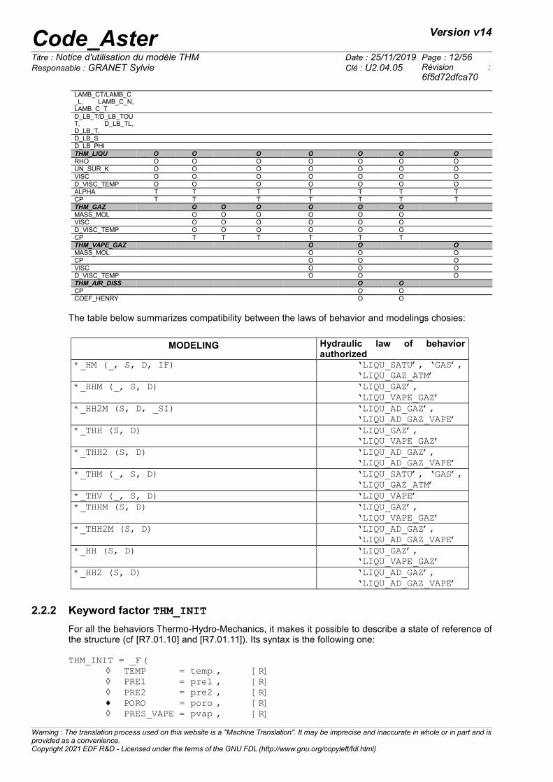
The table below summarizes compatibility between the laws of behavior and modelings chosies:
MODELING Hydraulic law of behavior
authorized *_HM (_, S, D, IF) ‘LIQU_SATU’, ‘GAS’,
‘LIQU_GAZ_ATM’*_HHM (_, S, D) ‘LIQU_GAZ’,
‘LIQU_VAPE_GAZ’*_HH2M (S, D, _SI) ‘LIQU_AD_GAZ’,
‘LIQU_AD_GAZ_VAPE’*_THH (S, D) ‘LIQU_GAZ’,
‘LIQU_VAPE_GAZ’*_THH2 (S, D) ‘LIQU_AD_GAZ’,
‘LIQU_AD_GAZ_VAPE’*_THM (_, S, D) ‘LIQU_SATU’, ‘GAS’,
‘LIQU_GAZ_ATM’*_THV (_, S, D) ‘LIQU_VAPE’*_THHM (S, D) ‘LIQU_GAZ’,
‘LIQU_VAPE_GAZ’*_THH2M (S, D) ‘LIQU_AD_GAZ’,
‘LIQU_AD_GAZ_VAPE’*_HH (S, D) ‘LIQU_GAZ’,
‘LIQU_VAPE_GAZ’*_HH2 (S, D) ‘LIQU_AD_GAZ’,
‘LIQU_AD_GAZ_VAPE’
2.2.2 Keyword factor THM_INIT
For all the behaviors Thermo-Hydro-Mechanics, it makes it possible to describe a state of reference ofthe structure (cf [R7.01.10] and [R7.01.11]). Its syntax is the following one:
THM_INIT = _F(◊ TEMP = temp , [R]◊ PRE1 = pre1 , [R]◊ PRE2 = pre2 , [R]♦ PORO = poro , [R]◊ PRES_VAPE = pvap , [R]
Warning : The translation process used on this website is a "Machine Translation". It may be imprecise and inaccurate in whole or in part and isprovided as a convenience.Copyright 2021 EDF R&D - Licensed under the terms of the GNU FDL (http://www.gnu.org/copyleft/fdl.html)
Code_Aster Version v14
Titre : Notice d'utilisation du modèle THM Date : 25/11/2019 Page : 13/56Responsable : GRANET Sylvie Clé : U2.04.05 Révision :
6f5d72dfca70
)
Under this keyword, there are three sizes corresponding to degrees of freedom. For understandingthese data well, it is necessary then to distinguish the unknown factors with the nodes, which we call
{u }ddl and values defined under the keyword THM_INIT that us appelonS p
ref and T ref
{u }ddl= {
ux
uy
uz
PRE1ddl
PRE2ddl
T ddl}
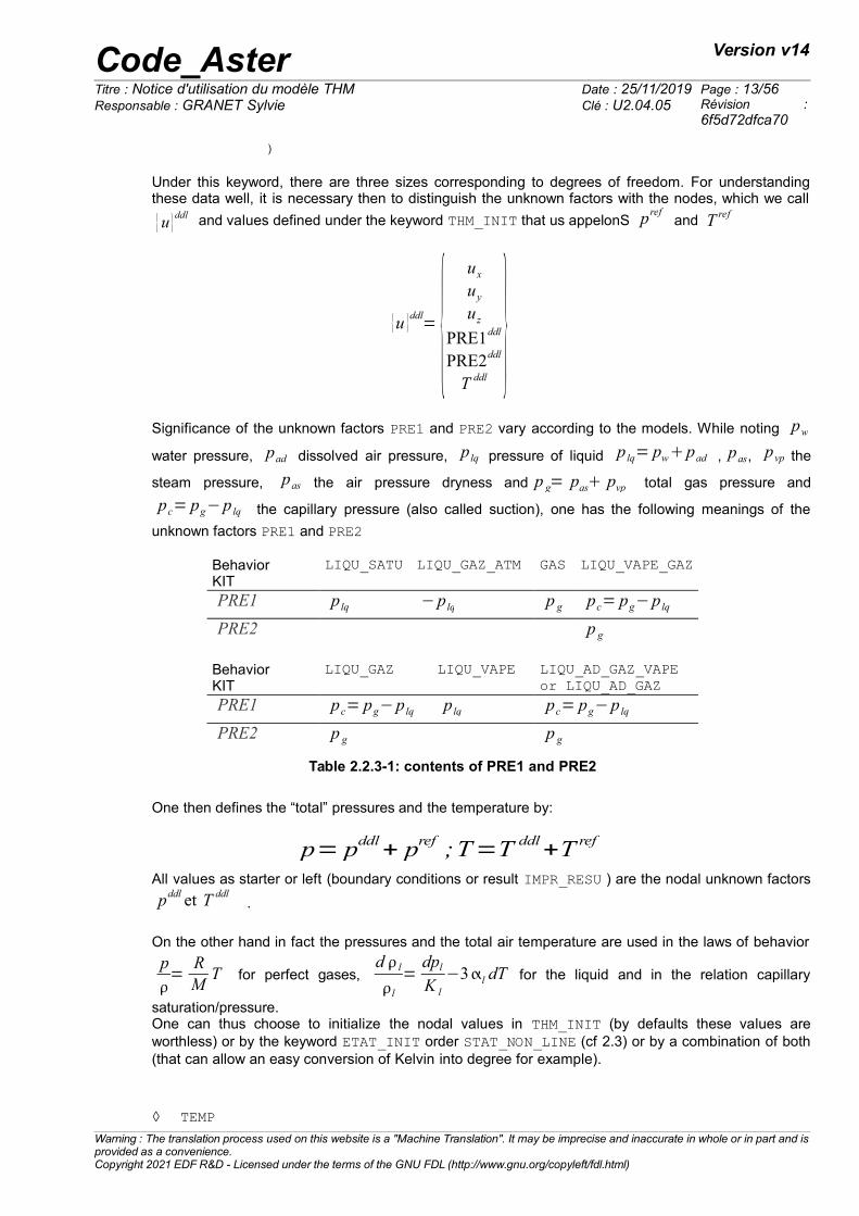
Significance of the unknown factors PRE1 and PRE2 vary according to the models. While noting pw
water pressure, pad dissolved air pressure, p lq pressure of liquid p lq= pwpad , pas, pvp the
steam pressure, pas the air pressure dryness and p g= pas pvp total gas pressure and
pc= pg−p lq the capillary pressure (also called suction), one has the following meanings of the
unknown factors PRE1 and PRE2
BehaviorKIT
LIQU_SATU LIQU_GAZ_ATM GAS LIQU_VAPE_GAZ
PRE1 p lq −p lq p g pc= pg−p lq
PRE2 p g
BehaviorKIT
LIQU_GAZ LIQU_VAPE LIQU_AD_GAZ_VAPEor LIQU_AD_GAZ
PRE1 pc= pg−p lq p lq pc= pg−p lq
PRE2 p g p g
Table 2.2.3-1: contents of PRE1 and PRE2
One then defines the “total” pressures and the temperature by:
p= pddl+ pref ;T=T ddl
+T ref
All values as starter or left (boundary conditions or result IMPR_RESU ) are the nodal unknown factors
pddl et T ddl .
On the other hand in fact the pressures and the total air temperature are used in the laws of behavior
p=
RM
T for perfect gases, d l
l
=dpl
K l
−3l dT for the liquid and in the relation capillary
saturation/pressure. One can thus choose to initialize the nodal values in THM_INIT (by defaults these values areworthless) or by the keyword ETAT_INIT order STAT_NON_LINE (cf 2.3) or by a combination of both(that can allow an easy conversion of Kelvin into degree for example).
◊ TEMP
Warning : The translation process used on this website is a "Machine Translation". It may be imprecise and inaccurate in whole or in part and isprovided as a convenience.Copyright 2021 EDF R&D - Licensed under the terms of the GNU FDL (http://www.gnu.org/copyleft/fdl.html)
Code_Aster Version v14
Titre : Notice d'utilisation du modèle THM Date : 25/11/2019 Page : 14/56Responsable : GRANET Sylvie Clé : U2.04.05 Révision :
6f5d72dfca70
Temperature of reference T ref . By default it is taken equalizes to zero. Attention the value of the
temperature initial T=T ddl+T ref must be strictly higher than zero.
◊ PRE1
By default it is taken equalizes to zero. As seen in table 1: For the behaviors LIQU_SATU , and LIQU_VAPE pressure of liquid of reference. For the behavior GAS gas pressure of ref.érence. In this case pressure initial gas
p= pddl+ pref must be nonworthless.
For the behavior LIQU_GAZ_ATM pressure of liquid of changed reference of sign. For the behaviors LIQU_VAPE_GAZ , LIQU_AD_GAZ, LIQU_AD_GAZ_VAPE and LIQU_GAZcapillary pressure of reference.
◊ PRE2
By default it is taken equalizes to zero. For the behaviors LIQU_VAPE_GAZ, LIQU_AD_GAZ,LIQU_AD_GAZ_VAPE and LIQU_GAZ standard gas pressure. pressure initial gas
p= pddl+ pref must be nonworthless.
♦ PORO
Initial porosity.♦ PRES_VAPE
Steam pressure of reference for the behaviors: LIQU_VAPE_GAZ, LIQU_AD_GAZ_VAPE andLIQU_VAPE.
Note:
The initial vapor pressure must be taken in coherence with other data. Very often, oneleaves the knowledge of an initial state of hygroscopy. The relative humidity is therelationship between the steam pressure and the steam pressure saturating at thetemperature considered. One then uses the law of Kelvin which gives the pressure of theliquid according to the steam pressure, of the temperature and the saturating steam
pressure:pw− pw
ref
w
=R
M vpol T ln pvp
pvpsatT . This relation is valid only for isothermal
evolutions. It is stressed that pwref
corresponds in a state of ‘balance to which
corresponds p pvsat
, this state of balance corresponds in fact to pw0= pgz
0=1atm . For
evolutions with temperature variation, knowing a law giving the steam pressure
saturating to the temperature T 0 , for example: p pvsatT 0=10
2.7858T0−273.5
31.5590.1354T0−273.5 , and a degree of hygroscopy HR , one from of deduced the steam pressure thanks to
p pv T 0=HR p pvsatT 0 .
Moreover, one never should take a value of PRES_VAPE equalize to zero.
2.2.3 Keyword factor THM_LIQU
This keyword relates to all behaviors THM utilizing a liquid (confer [R7.01.11]). Its syntax is thefollowing one:
THM_LIQU = _F( ♦ RHO = rho , [R]
Warning : The translation process used on this website is a "Machine Translation". It may be imprecise and inaccurate in whole or in part and isprovided as a convenience.Copyright 2021 EDF R&D - Licensed under the terms of the GNU FDL (http://www.gnu.org/copyleft/fdl.html)
Code_Aster Version v14
Titre : Notice d'utilisation du modèle THM Date : 25/11/2019 Page : 15/56Responsable : GRANET Sylvie Clé : U2.04.05 Révision :
6f5d72dfca70
♦ UN_SUR_K = usk , [R]♦ VISC = VI , [function **]♦ D_VISC_TEMP = dvi , [function **]◊ ALPHA = alp , [R]◊ CP = CP , [R])
♦ RHO
Density initial liquidE.
♦ UN_SUR_K
Opposite of the compressibility of the liquid: K l .♦ VISC [function **]
Viscosity of the liquid. Function of the temperature.
♦ D_VISC_TEMP [function **]
Derived from the viscosity of the liquid compared to the temperature. Function of thetemperature. The user must ensure coherence with the function associated with VISC.
◊ ALPHA
Dilation coefficient (linear) of the liquid l
If p l indicate the pressure of the liquid, l its density and T the temperature, the behavior of
the liquid is: dρl
l
=dpl
K l
−3ldT
◊ CP
Specific heat with constant pressure of the liquid.
2.2.4 Keyword factor THM_GAZ
This keyword factor relates to all behaviors THM utilizing a gas (cf [R7.01.11]). For the behaviorsutilizing at the same time a liquid and a gas, and when one takes into account the evaporation of theliquid, the coefficients indicated here relate to dry gas. The properties of the vapor will be indicatedunder the keyword THM_VAPE_GAZ. Its syntax is the following one:
THM_GAZ = _F (
♦ MASS_MOL = Mgs , [R] ♦ CP = CP , [R]♦ VISC = VI , [function **]♦ D_VISC_TEMP = dvi , [function **]
)
♦ MASS_MOL
Molar mass of dry gas. M gs
If p gs indicate the pressure of dry gas, gs its density, R the constant of perfect gases and T
the temperature, the reaction of dry gas is: pgs
gs
=RTM gs
.
♦ CP
Specific heat with constant pressure of dry gas.
Warning : The translation process used on this website is a "Machine Translation". It may be imprecise and inaccurate in whole or in part and isprovided as a convenience.Copyright 2021 EDF R&D - Licensed under the terms of the GNU FDL (http://www.gnu.org/copyleft/fdl.html)
Code_Aster Version v14
Titre : Notice d'utilisation du modèle THM Date : 25/11/2019 Page : 16/56Responsable : GRANET Sylvie Clé : U2.04.05 Révision :
6f5d72dfca70
♦ VISC [function **]
Viscosity of dry gas. Function of the temperature.
♦ D_VISC_TEMP [function **]
Derived compared to the temperature from viscosity from dry gas. Function of the temperature.The user must ensure coherence with the function associated with VISC.
2.2.5 Keyword factor THM_VAPE_GAZ
This keyword factor relates to all behaviors THM utilizing at the same time a liquid and a gas, andfascinating of account the evaporation of the liquid (cf [R7.01.11]). The coefficients indicated hererelate to the vapor. Syntax is the following one:
THM_VAPE_GAZ = _F (
♦ MASS_MOL = m , [R] ♦ CP = CP , [R]♦ VISC = VI , [function **]♦ D_VISC_TEMP = dvi , [function **]
)♦ MASS_MOL
Molar mass of the vapor. M vp
♦ CP
Specific heat with constant pressure of the vapor.
♦ VISC [function **]
Viscosity of the vapor. Function of the temperature.
♦ D_VISC_TEMP [function **]
Derived compared to the temperature from viscosity from the vapor. Function of the temperature.The user must ensure coherence with the function associated with VISC.
2.2.6 Keyword factor THM_AIR_DISS
This keyword factor relates to behavior THM THM_AIR_DISS taking into account the dissolution of theair in the liquid (cf [R7.01.11]). The coefficients indicated here relate to the dissolved air. Syntax is thefollowing one:
THM_AIR_DISS = _F (
♦ CP = CP , [R] ♦ COEF_HENRY = KH , [function **]
)
♦ CP
Specific heat with constant pressure of the dissolved air.
♦ COEF_HENRY
Constant of Henry K H , allowing to connect the molar concentration of dissolved air Cadol
(
moles /m3 ) with the air pressure dryness:
Cadol=
pas
K H
Note:Warning : The translation process used on this website is a "Machine Translation". It may be imprecise and inaccurate in whole or in part and isprovided as a convenience.Copyright 2021 EDF R&D - Licensed under the terms of the GNU FDL (http://www.gnu.org/copyleft/fdl.html)
Code_Aster Version v14
Titre : Notice d'utilisation du modèle THM Date : 25/11/2019 Page : 17/56Responsable : GRANET Sylvie Clé : U2.04.05 Révision :
6f5d72dfca70
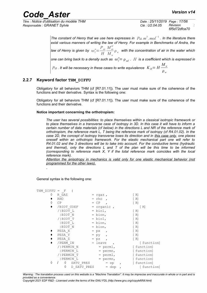
The constant of Henry that we use here expresses in Pa.m3 .mol−1 . In the literature thereexist various manners of writing the law of Henry. For example in Benchmarks of Andra, the
law of Henry is given by la=
Pas
H
M asol
M w
w with the concentration of air in the water which
one can bring back to a density such as la= ad . H is a coefficient which is expressed in
Pa . It will be necessary in these cases to write equivalence K H= HM w
w
2.2.7 Keyword factor THM_DIFFU
Obligatory for all behaviors THM (cf [R7.01.11]). The user must make sure of the coherence of thefunctions and their derivative. Syntax is the following one:
Obligatory for all behaviors THM (cf [R7.01.11]). The user must make sure of the coherence of thefunctions and their derivative.
Notice important concerning the orthotropism:
The user has several possibilities: to place themselves within a classical isotropic framework orto place themselves in a transverse case of isotropy in 3D. In this case it will have to inform acertain number of data materials (cf below) in the directions L and NR of the reference mark oforthotropism, the reference mark L, T being the reference mark of isotropy (cf R4.01.02). In thecase 2D, the concept of isotropy transverse loses its direction and in this case only, one placesoneself within an orthotropic framework. For the elastic mechanical part one will refer toR4.01.02 and the 3 directions will be to take into account. For the conductive terms (hydraulicand thermal), only the directions L and T of the plan will be this time to be informed(corresponding to reference mark X, Y if the total reference mark coincides with the localreference mark).Attention the anisotropy in mechanics is valid only for one elastic mechanical behavior (notprogrammed for the other laws).
General syntax is the following one:
THM_DIFFU = _F ( ◊ R_GAZ = rgaz , [R] ♦ RHO = rho , [R] ◊ CP = CP , [R] ♦ /BIOT_COEF = organic , [R]
/|BIOT_L = biol, [R] |BIOT_N = bion, [R]
/|BIOT_T = biol, [R] |BIOT_L = bion, [R] |BIOT_N = bion, [R]
♦ PESA_X = px , [R]♦ PESA_Y = py , [R]♦ PESA_Z = pz , [R]
♦ /PERM_IN = leave , [function] /|PERMIN_N = perml, [function]
|PERMIN_L = permn, [function] /|PERMIN_T = perml, [function]
|PERMIN_L = permn, [function]◊ / ◊ SATU_PRES = sp , [function]
◊ D_SATU_PRES = dsp , [function]
Warning : The translation process used on this website is a "Machine Translation". It may be imprecise and inaccurate in whole or in part and isprovided as a convenience.Copyright 2021 EDF R&D - Licensed under the terms of the GNU FDL (http://www.gnu.org/copyleft/fdl.html)
Code_Aster Version v14
Titre : Notice d'utilisation du modèle THM Date : 25/11/2019 Page : 18/56Responsable : GRANET Sylvie Clé : U2.04.05 Révision :
6f5d72dfca70
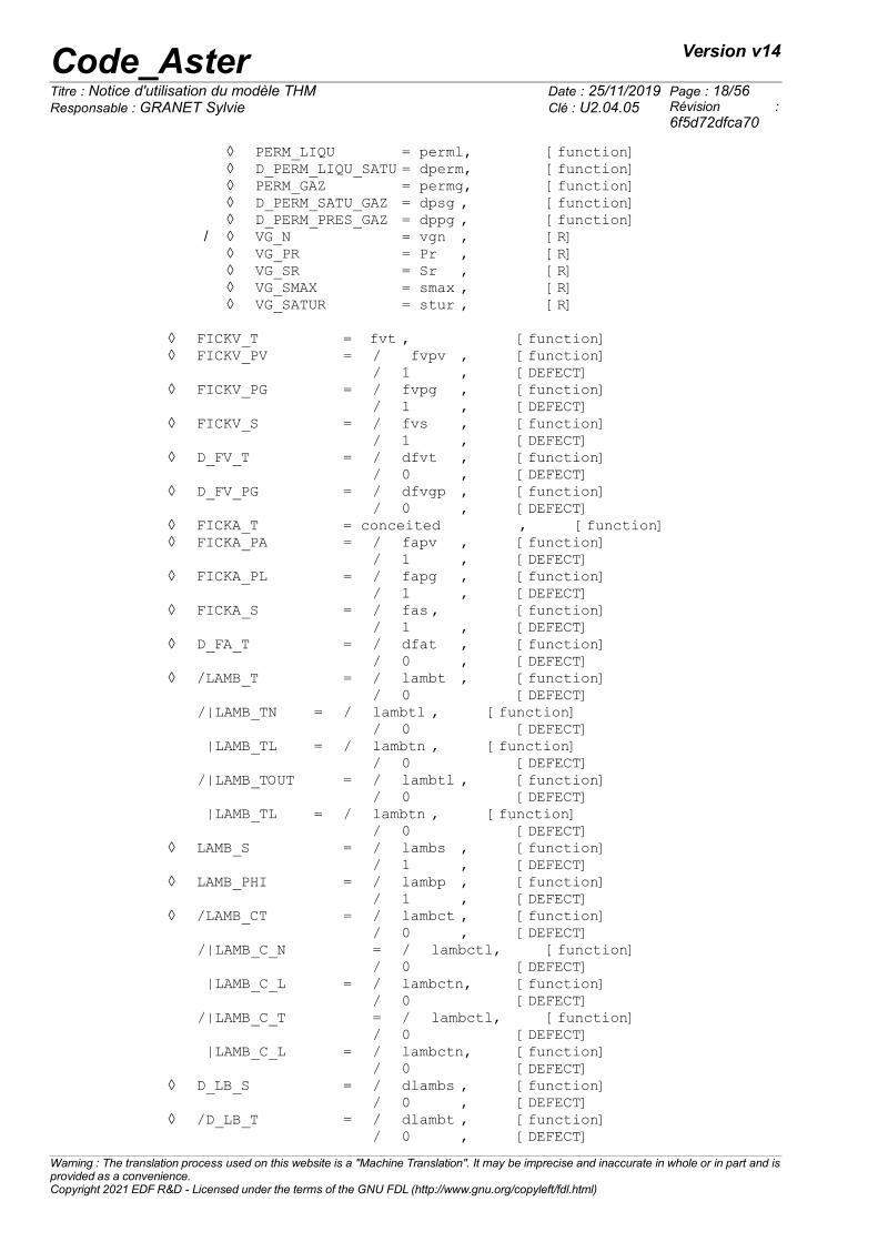
◊ PERM_LIQU = perml, [function]◊ D_PERM_LIQU_SATU = dperm, [function]◊ PERM_GAZ = permg, [function]◊ D_PERM_SATU_GAZ = dpsg , [function]◊ D_PERM_PRES_GAZ = dppg , [function]
/ ◊ VG_N = vgn , [R] ◊ VG_PR = Pr , [R] ◊ VG_SR = Sr , [R] ◊ VG_SMAX = smax , [R] ◊ VG_SATUR = stur , [R]
◊ FICKV_T = fvt , [function]◊ FICKV_PV = / fvpv , [function]
/ 1 , [DEFECT]◊ FICKV_PG = / fvpg , [function]
/ 1 , [DEFECT]◊ FICKV_S = / fvs , [function]
/ 1 , [DEFECT]◊ D_FV_T = / dfvt , [function]
/ 0 , [DEFECT]◊ D_FV_PG = / dfvgp , [function]
/ 0 , [DEFECT]◊ FICKA_T = conceited , [function]◊ FICKA_PA = / fapv , [function]
/ 1 , [DEFECT]◊ FICKA_PL = / fapg , [function]
/ 1 , [DEFECT]◊ FICKA_S = / fas , [function]
/ 1 , [DEFECT]◊ D_FA_T = / dfat , [function]
/ 0 , [DEFECT]◊ /LAMB_T = / lambt , [function]
/ 0 [DEFECT] /|LAMB_TN = / lambtl , [function]
/ 0 [DEFECT] |LAMB_TL = / lambtn , [function]
/ 0 [DEFECT] /|LAMB_TOUT = / lambtl , [function]
/ 0 [DEFECT] |LAMB_TL = / lambtn , [function]
/ 0 [DEFECT]◊ LAMB_S = / lambs , [function]
/ 1 , [DEFECT]◊ LAMB_PHI = / lambp , [function]
/ 1 , [DEFECT]◊ /LAMB_CT = / lambct , [function]
/ 0 , [DEFECT] /|LAMB_C_N = / lambctl, [function]
/ 0 [DEFECT] |LAMB_C_L = / lambctn, [function]
/ 0 [DEFECT] /|LAMB_C_T = / lambctl, [function]
/ 0 [DEFECT] |LAMB_C_L = / lambctn, [function]
/ 0 [DEFECT]◊ D_LB_S = / dlambs , [function]
/ 0 , [DEFECT]◊ /D_LB_T = / dlambt , [function]
/ 0 , [DEFECT]
Warning : The translation process used on this website is a "Machine Translation". It may be imprecise and inaccurate in whole or in part and isprovided as a convenience.Copyright 2021 EDF R&D - Licensed under the terms of the GNU FDL (http://www.gnu.org/copyleft/fdl.html)
Code_Aster Version v14
Titre : Notice d'utilisation du modèle THM Date : 25/11/2019 Page : 19/56Responsable : GRANET Sylvie Clé : U2.04.05 Révision :
6f5d72dfca70
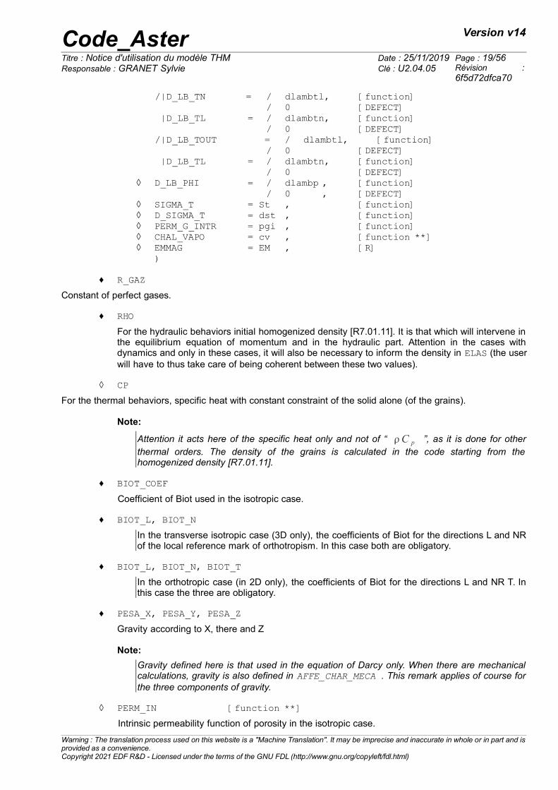
/|D_LB_TN = / dlambtl, [function]/ 0 [DEFECT]
|D_LB_TL = / dlambtn, [function]/ 0 [DEFECT]
/|D_LB_TOUT = / dlambtl, [function]/ 0 [DEFECT]
|D_LB_TL = / dlambtn, [function]/ 0 [DEFECT]
◊ D_LB_PHI = / dlambp , [function]/ 0 , [DEFECT]
◊ SIGMA_T = St , [function]◊ D_SIGMA_T = dst , [function]◊ PERM_G_INTR = pgi , [function]◊ CHAL_VAPO = cv , [function **]◊ EMMAG = EM , [R]
)
♦ R_GAZ
Constant of perfect gases.
♦ RHO
For the hydraulic behaviors initial homogenized density [R7.01.11]. It is that which will intervene inthe equilibrium equation of momentum and in the hydraulic part. Attention in the cases withdynamics and only in these cases, it will also be necessary to inform the density in ELAS (the userwill have to thus take care of being coherent between these two values).
◊ CP
For the thermal behaviors, specific heat with constant constraint of the solid alone (of the grains).
Note:
Attention it acts here of the specific heat only and not of “ C p ”, as it is done for otherthermal orders. The density of the grains is calculated in the code starting from thehomogenized density [R7.01.11].
♦ BIOT_COEF
Coefficient of Biot used in the isotropic case.
♦ BIOT_L, BIOT_N
In the transverse isotropic case (3D only), the coefficients of Biot for the directions L and NRof the local reference mark of orthotropism. In this case both are obligatory.
♦ BIOT_L, BIOT_N, BIOT_T
In the orthotropic case (in 2D only), the coefficients of Biot for the directions L and NR T. Inthis case the three are obligatory.
♦ PESA_X, PESA_Y, PESA_Z
Gravity according to X, there and Z
Note:
Gravity defined here is that used in the equation of Darcy only. When there are mechanicalcalculations, gravity is also defined in AFFE_CHAR_MECA . This remark applies of course forthe three components of gravity.
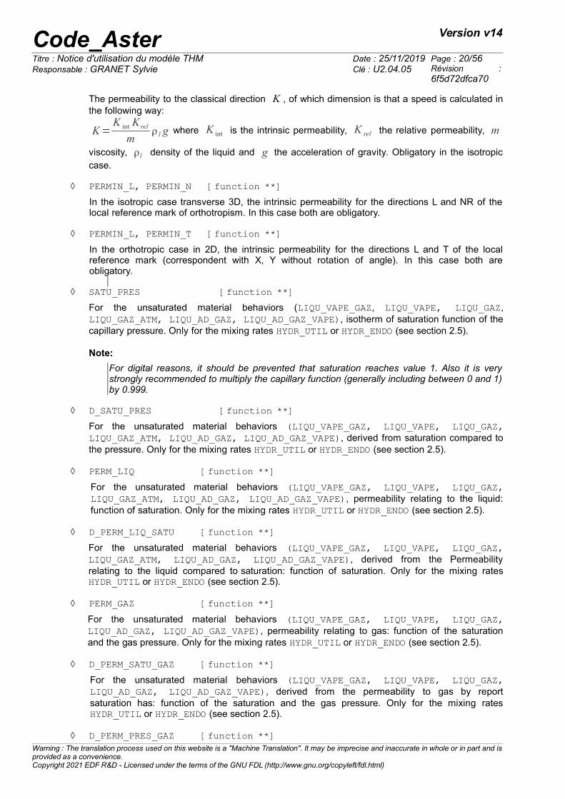
◊ PERM_IN [function **]
Intrinsic permeability function of porosity in the isotropic case.
Warning : The translation process used on this website is a "Machine Translation". It may be imprecise and inaccurate in whole or in part and isprovided as a convenience.Copyright 2021 EDF R&D - Licensed under the terms of the GNU FDL (http://www.gnu.org/copyleft/fdl.html)
Code_Aster Version v14
Titre : Notice d'utilisation du modèle THM Date : 25/11/2019 Page : 20/56Responsable : GRANET Sylvie Clé : U2.04.05 Révision :
6f5d72dfca70
The permeability to the classical direction K , of which dimension is that a speed is calculated inthe following way:
K=K int K rel
m l g where K int is the intrinsic permeability, K rel the relative permeability, m
viscosity, l density of the liquid and g the acceleration of gravity. Obligatory in the isotropiccase.
◊ PERMIN_L, PERMIN_N [function **]
In the isotropic case transverse 3D, the intrinsic permeability for the directions L and NR of thelocal reference mark of orthotropism. In this case both are obligatory.
◊ PERMIN_L, PERMIN_T [function **]
In the orthotropic case in 2D, the intrinsic permeability for the directions L and T of the localreference mark (correspondent with X, Y without rotation of angle). In this case both areobligatory.
◊ SATU_PRES [function **]
For the unsaturated material behaviors (LIQU_VAPE_GAZ, LIQU_VAPE, LIQU_GAZ,LIQU_GAZ_ATM, LIQU_AD_GAZ, LIQU_AD_GAZ_VAPE), isotherm of saturation function of thecapillary pressure. Only for the mixing rates HYDR_UTIL or HYDR_ENDO (see section 2.5).
Note:
For digital reasons, it should be prevented that saturation reaches value 1. Also it is verystrongly recommended to multiply the capillary function (generally including between 0 and 1)by 0.999.
◊ D_SATU_PRES [function **]
For the unsaturated material behaviors (LIQU_VAPE_GAZ, LIQU_VAPE, LIQU_GAZ,LIQU_GAZ_ATM, LIQU_AD_GAZ, LIQU_AD_GAZ_VAPE), derived from saturation compared tothe pressure. Only for the mixing rates HYDR_UTIL or HYDR_ENDO (see section 2.5).
◊ PERM_LIQ [function **]
For the unsaturated material behaviors (LIQU_VAPE_GAZ, LIQU_VAPE, LIQU_GAZ,LIQU_GAZ_ATM, LIQU_AD_GAZ, LIQU_AD_GAZ_VAPE), permeability relating to the liquid:function of saturation. Only for the mixing rates HYDR_UTIL or HYDR_ENDO (see section 2.5).
◊ D_PERM_LIQ_SATU [function **]
For the unsaturated material behaviors (LIQU_VAPE_GAZ, LIQU_VAPE, LIQU_GAZ,LIQU_GAZ_ATM, LIQU_AD_GAZ, LIQU_AD_GAZ_VAPE), derived from the Permeabilityrelating to the liquid compared to saturation: function of saturation. Only for the mixing ratesHYDR_UTIL or HYDR_ENDO (see section 2.5).
◊ PERM_GAZ [function **]
For the unsaturated material behaviors (LIQU_VAPE_GAZ, LIQU_VAPE, LIQU_GAZ,LIQU_AD_GAZ, LIQU_AD_GAZ_VAPE), permeability relating to gas: function of the saturationand the gas pressure. Only for the mixing rates HYDR_UTIL or HYDR_ENDO (see section 2.5).
◊ D_PERM_SATU_GAZ [function **]
For the unsaturated material behaviors (LIQU_VAPE_GAZ, LIQU_VAPE, LIQU_GAZ,LIQU_AD_GAZ, LIQU_AD_GAZ_VAPE), derived from the permeability to gas by reportsaturation has: function of the saturation and the gas pressure. Only for the mixing ratesHYDR_UTIL or HYDR_ENDO (see section 2.5).
◊ D_PERM_PRES_GAZ [function **]Warning : The translation process used on this website is a "Machine Translation". It may be imprecise and inaccurate in whole or in part and isprovided as a convenience.Copyright 2021 EDF R&D - Licensed under the terms of the GNU FDL (http://www.gnu.org/copyleft/fdl.html)
Code_Aster Version v14
Titre : Notice d'utilisation du modèle THM Date : 25/11/2019 Page : 21/56Responsable : GRANET Sylvie Clé : U2.04.05 Révision :
6f5d72dfca70
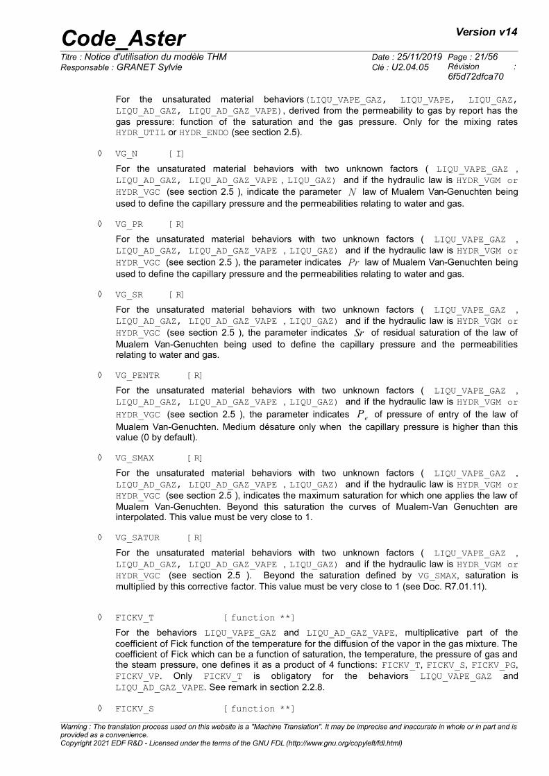
For the unsaturated material behaviors(LIQU_VAPE_GAZ, LIQU_VAPE, LIQU_GAZ,LIQU_AD_GAZ, LIQU_AD_GAZ_VAPE), derived from the permeability to gas by report has thegas pressure: function of the saturation and the gas pressure. Only for the mixing ratesHYDR_UTIL or HYDR_ENDO (see section 2.5).
◊ VG_N [I]
For the unsaturated material behaviors with two unknown factors ( LIQU_VAPE_GAZ ,LIQU_AD_GAZ, LIQU_AD_GAZ_VAPE , LIQU_GAZ) and if the hydraulic law is HYDR_VGM orHYDR_VGC (see section 2.5 ), indicate the parameter N law of Mualem Van-Genuchten beingused to define the capillary pressure and the permeabilities relating to water and gas.
◊ VG_PR [R]
For the unsaturated material behaviors with two unknown factors ( LIQU_VAPE_GAZ ,LIQU_AD_GAZ, LIQU_AD_GAZ_VAPE , LIQU_GAZ) and if the hydraulic law is HYDR_VGM orHYDR_VGC (see section 2.5 ), the parameter indicates Pr law of Mualem Van-Genuchten beingused to define the capillary pressure and the permeabilities relating to water and gas.
◊ VG_SR [R]
For the unsaturated material behaviors with two unknown factors ( LIQU_VAPE_GAZ ,LIQU_AD_GAZ, LIQU_AD_GAZ_VAPE , LIQU_GAZ) and if the hydraulic law is HYDR_VGM orHYDR_VGC (see section 2.5 ), the parameter indicates Sr of residual saturation of the law ofMualem Van-Genuchten being used to define the capillary pressure and the permeabilitiesrelating to water and gas.
◊ VG_PENTR [R]
For the unsaturated material behaviors with two unknown factors ( LIQU_VAPE_GAZ ,LIQU_AD_GAZ, LIQU_AD_GAZ_VAPE , LIQU_GAZ) and if the hydraulic law is HYDR_VGM orHYDR_VGC (see section 2.5 ), the parameter indicates P e of pressure of entry of the law ofMualem Van-Genuchten. Medium désature only when the capillary pressure is higher than thisvalue (0 by default).
◊ VG_SMAX [R]
For the unsaturated material behaviors with two unknown factors ( LIQU_VAPE_GAZ ,LIQU_AD_GAZ, LIQU_AD_GAZ_VAPE , LIQU_GAZ) and if the hydraulic law is HYDR_VGM orHYDR_VGC (see section 2.5 ), indicates the maximum saturation for which one applies the law ofMualem Van-Genuchten. Beyond this saturation the curves of Mualem-Van Genuchten areinterpolated. This value must be very close to 1.
◊ VG_SATUR [R]
For the unsaturated material behaviors with two unknown factors ( LIQU_VAPE_GAZ ,LIQU_AD_GAZ, LIQU_AD_GAZ_VAPE , LIQU_GAZ) and if the hydraulic law is HYDR_VGM orHYDR_VGC (see section 2.5 ). Beyond the saturation defined by VG_SMAX, saturation ismultiplied by this corrective factor. This value must be very close to 1 (see Doc. R7.01.11).
◊ FICKV_T [function **]
For the behaviors LIQU_VAPE_GAZ and LIQU_AD_GAZ_VAPE, multiplicative part of thecoefficient of Fick function of the temperature for the diffusion of the vapor in the gas mixture. Thecoefficient of Fick which can be a function of saturation, the temperature, the pressure of gas andthe steam pressure, one defines it as a product of 4 functions: FICKV_T, FICKV_S, FICKV_PG,FICKV_VP. Only FICKV_T is obligatory for the behaviors LIQU_VAPE_GAZ andLIQU_AD_GAZ_VAPE. See remark in section 2.2.8.
◊ FICKV_S [function **]
Warning : The translation process used on this website is a "Machine Translation". It may be imprecise and inaccurate in whole or in part and isprovided as a convenience.Copyright 2021 EDF R&D - Licensed under the terms of the GNU FDL (http://www.gnu.org/copyleft/fdl.html)
Code_Aster Version v14
Titre : Notice d'utilisation du modèle THM Date : 25/11/2019 Page : 22/56Responsable : GRANET Sylvie Clé : U2.04.05 Révision :
6f5d72dfca70
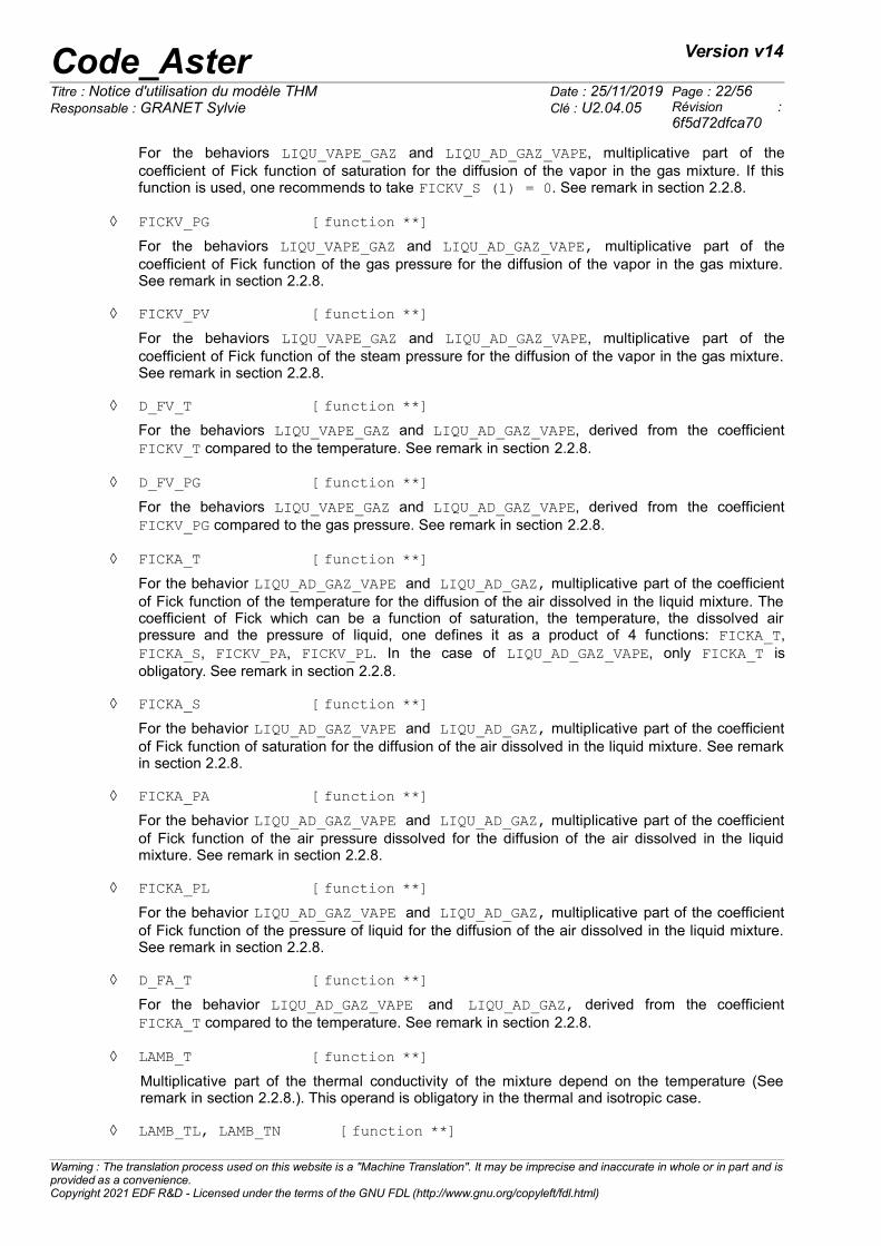
For the behaviors LIQU_VAPE_GAZ and LIQU_AD_GAZ_VAPE, multiplicative part of thecoefficient of Fick function of saturation for the diffusion of the vapor in the gas mixture. If thisfunction is used, one recommends to take FICKV_S (1) = 0. See remark in section 2.2.8.
◊ FICKV_PG [function **]
For the behaviors LIQU_VAPE_GAZ and LIQU_AD_GAZ_VAPE, multiplicative part of thecoefficient of Fick function of the gas pressure for the diffusion of the vapor in the gas mixture.See remark in section 2.2.8.
◊ FICKV_PV [function **]
For the behaviors LIQU_VAPE_GAZ and LIQU_AD_GAZ_VAPE, multiplicative part of thecoefficient of Fick function of the steam pressure for the diffusion of the vapor in the gas mixture.See remark in section 2.2.8.
◊ D_FV_T [function **]
For the behaviors LIQU_VAPE_GAZ and LIQU_AD_GAZ_VAPE, derived from the coefficientFICKV_T compared to the temperature. See remark in section 2.2.8.
◊ D_FV_PG [function **]
For the behaviors LIQU_VAPE_GAZ and LIQU_AD_GAZ_VAPE, derived from the coefficientFICKV_PG compared to the gas pressure. See remark in section 2.2.8.
◊ FICKA_T [function **]
For the behavior LIQU_AD_GAZ_VAPE and LIQU_AD_GAZ, multiplicative part of the coefficientof Fick function of the temperature for the diffusion of the air dissolved in the liquid mixture. Thecoefficient of Fick which can be a function of saturation, the temperature, the dissolved airpressure and the pressure of liquid, one defines it as a product of 4 functions: FICKA_T,FICKA_S, FICKV_PA, FICKV_PL. In the case of LIQU_AD_GAZ_VAPE, only FICKA_T isobligatory. See remark in section 2.2.8.
◊ FICKA_S [function **]
For the behavior LIQU_AD_GAZ_VAPE and LIQU_AD_GAZ, multiplicative part of the coefficientof Fick function of saturation for the diffusion of the air dissolved in the liquid mixture. See remarkin section 2.2.8.
◊ FICKA_PA [function **]
For the behavior LIQU_AD_GAZ_VAPE and LIQU_AD_GAZ, multiplicative part of the coefficientof Fick function of the air pressure dissolved for the diffusion of the air dissolved in the liquidmixture. See remark in section 2.2.8.
◊ FICKA_PL [function **]
For the behavior LIQU_AD_GAZ_VAPE and LIQU_AD_GAZ, multiplicative part of the coefficientof Fick function of the pressure of liquid for the diffusion of the air dissolved in the liquid mixture.See remark in section 2.2.8.
◊ D_FA_T [function **]
For the behavior LIQU_AD_GAZ_VAPE and LIQU_AD_GAZ, derived from the coefficientFICKA_T compared to the temperature. See remark in section 2.2.8.
◊ LAMB_T [function **]
Multiplicative part of the thermal conductivity of the mixture depend on the temperature (Seeremark in section 2.2.8.). This operand is obligatory in the thermal and isotropic case.
◊ LAMB_TL, LAMB_TN [function **]
Warning : The translation process used on this website is a "Machine Translation". It may be imprecise and inaccurate in whole or in part and isprovided as a convenience.Copyright 2021 EDF R&D - Licensed under the terms of the GNU FDL (http://www.gnu.org/copyleft/fdl.html)
Code_Aster Version v14
Titre : Notice d'utilisation du modèle THM Date : 25/11/2019 Page : 23/56Responsable : GRANET Sylvie Clé : U2.04.05 Révision :
6f5d72dfca70
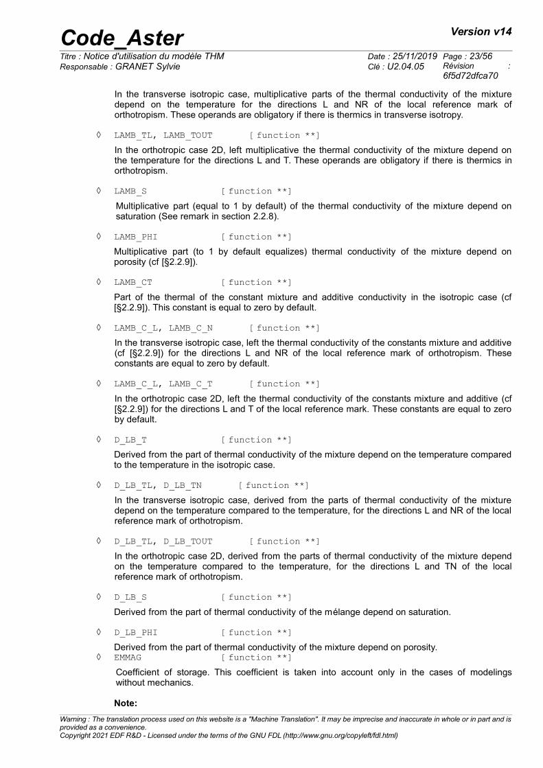
In the transverse isotropic case, multiplicative parts of the thermal conductivity of the mixturedepend on the temperature for the directions L and NR of the local reference mark oforthotropism. These operands are obligatory if there is thermics in transverse isotropy.
◊ LAMB_TL, LAMB_TOUT [function **]
In the orthotropic case 2D, left multiplicative the thermal conductivity of the mixture depend onthe temperature for the directions L and T. These operands are obligatory if there is thermics inorthotropism.
◊ LAMB_S [function **]
Multiplicative part (equal to 1 by default) of the thermal conductivity of the mixture depend onsaturation (See remark in section 2.2.8).
◊ LAMB_PHI [function **]
Multiplicative part (to 1 by default equalizes) thermal conductivity of the mixture depend onporosity (cf [§2.2.9]).
◊ LAMB_CT [function **]
Part of the thermal of the constant mixture and additive conductivity in the isotropic case (cf[§2.2.9]). This constant is equal to zero by default.
◊ LAMB_C_L, LAMB_C_N [function **]
In the transverse isotropic case, left the thermal conductivity of the constants mixture and additive(cf [§2.2.9]) for the directions L and NR of the local reference mark of orthotropism. Theseconstants are equal to zero by default.
◊ LAMB_C_L, LAMB_C_T [function **]
In the orthotropic case 2D, left the thermal conductivity of the constants mixture and additive (cf[§2.2.9]) for the directions L and T of the local reference mark. These constants are equal to zeroby default.
◊ D_LB_T [function **]
Derived from the part of thermal conductivity of the mixture depend on the temperature comparedto the temperature in the isotropic case.
◊ D_LB_TL, D_LB_TN [function **]
In the transverse isotropic case, derived from the parts of thermal conductivity of the mixturedepend on the temperature compared to the temperature, for the directions L and NR of the localreference mark of orthotropism.
◊ D_LB_TL, D_LB_TOUT [function **]
In the orthotropic case 2D, derived from the parts of thermal conductivity of the mixture dependon the temperature compared to the temperature, for the directions L and TN of the localreference mark of orthotropism.
◊ D_LB_S [function **]
Derived from the part of thermal conductivity of the mélange depend on saturation.
◊ D_LB_PHI [function **]
Derived from the part of thermal conductivity of the mixture depend on porosity.◊ EMMAG [function **]
Coefficient of storage. This coefficient is taken into account only in the cases of modelingswithout mechanics.
Note:
Warning : The translation process used on this website is a "Machine Translation". It may be imprecise and inaccurate in whole or in part and isprovided as a convenience.Copyright 2021 EDF R&D - Licensed under the terms of the GNU FDL (http://www.gnu.org/copyleft/fdl.html)
Code_Aster Version v14
Titre : Notice d'utilisation du modèle THM Date : 25/11/2019 Page : 24/56Responsable : GRANET Sylvie Clé : U2.04.05 Révision :
6f5d72dfca70
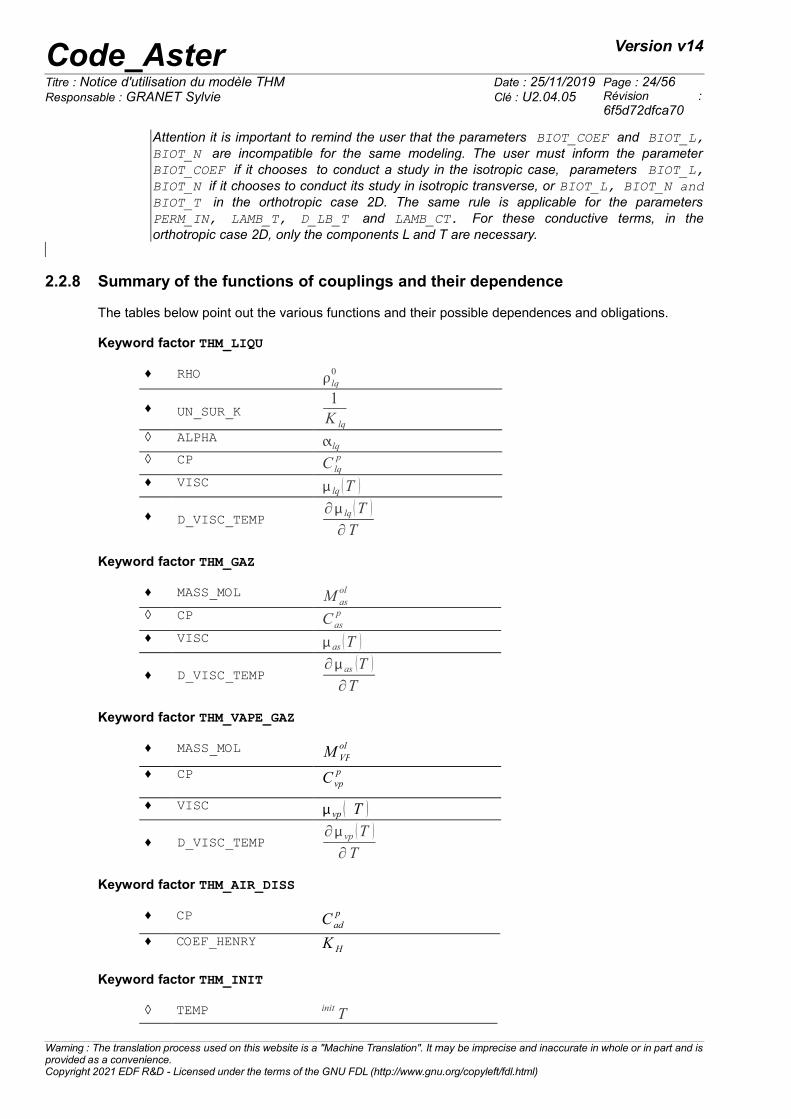
Attention it is important to remind the user that the parameters BIOT_COEF and BIOT_L,BIOT_N are incompatible for the same modeling. The user must inform the parameterBIOT_COEF if it chooses to conduct a study in the isotropic case, parameters BIOT_L,BIOT_N if it chooses to conduct its study in isotropic transverse, or BIOT_L, BIOT_N andBIOT_T in the orthotropic case 2D. The same rule is applicable for the parametersPERM_IN, LAMB_T, D_LB_T and LAMB_CT. For these conductive terms, in theorthotropic case 2D, only the components L and T are necessary.
2.2.8 Summary of the functions of couplings and their dependence
The tables below point out the various functions and their possible dependences and obligations.
Keyword factor THM_LIQU
♦ RHO lq0
♦ UN_SUR_K1K lq
◊ ALPHA lq ◊ CP C lq
p
♦ VISC lq T
♦ D_VISC_TEMP∂ lq T ∂T
Keyword factor THM_GAZ
♦ MASS_MOL M asol
◊ CP Cas
p
♦ VISC as T
♦ D_VISC_TEMP∂as T ∂T
Keyword factor THM_VAPE_GAZ
♦ MASS_MOL M VPol
♦ CP C vpp
♦ VISC vp T
♦ D_VISC_TEMP∂ vp T ∂T
Keyword factor THM_AIR_DISS
♦ CP Cadp
♦ COEF_HENRY K H
Keyword factor THM_INIT
◊ TEMP init T
Warning : The translation process used on this website is a "Machine Translation". It may be imprecise and inaccurate in whole or in part and isprovided as a convenience.Copyright 2021 EDF R&D - Licensed under the terms of the GNU FDL (http://www.gnu.org/copyleft/fdl.html)
Code_Aster Version v14
Titre : Notice d'utilisation du modèle THM Date : 25/11/2019 Page : 25/56Responsable : GRANET Sylvie Clé : U2.04.05 Révision :
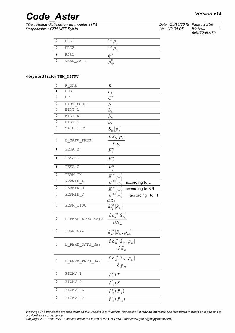
6f5d72dfca70
◊ PRE1 init P1 ◊ PRE2 init P2 ♦ PORO
0 ◊ NEAR_VAPE pvp
0
•Keyword factor THM_DIFFU
◊ R_GAZ R ♦ RHO r 0 ◊ CP C
s
◊ BIOT_COEF b ◊ BIOT_L bL ◊ BIOT_N bN ◊ BIOT_T bT ◊ SATU_PRES S lq pc
◊ D_SATU_PRES∂ S lq pc ∂ pc
♦ PESA_X F xm
♦ PESA_Y F ym
♦ PESA_Z F zm
◊ PERM_IN K int ◊ PERMIN_L K int according to L◊ PERMIN_N K int according to NR◊ PERMIN_T K int according to T
(2D)◊ PERM_LIQU k lq
rel S lq
◊ D_PERM_LIQU_SATU∂ k lq
rel S lq ∂ S lq
◊ PERM_GAZ k gzrel S lq , pgz
◊ D_PERM_SATU_GAZ∂ k gz
rel S lq , pgz ∂ S lq
◊ D_PERM_PRES_GAZ∂ k gz
rel S lq , pgz ∂ pgz
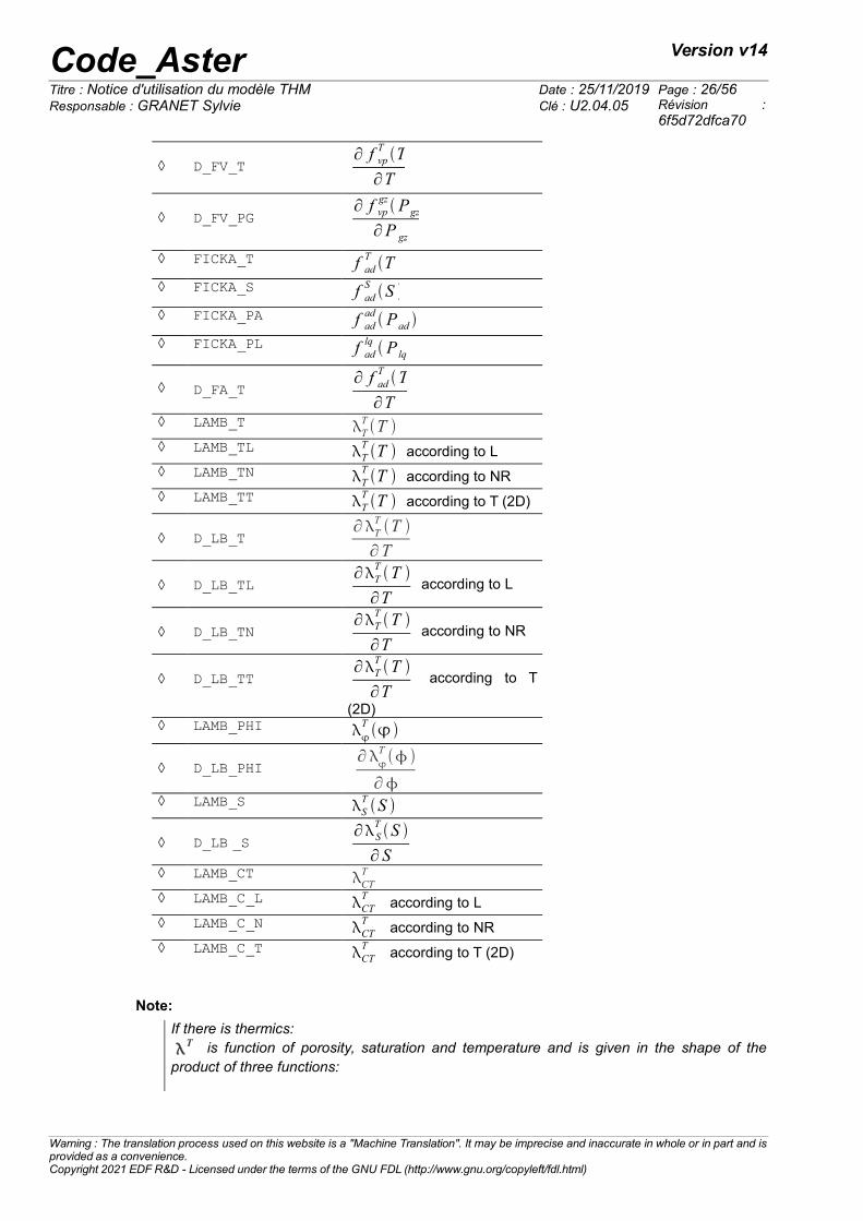
◊ FICKV_T f vpTT
◊ FICKV_S f vpSS
◊ FICKV_PG f vpgz Pg
◊ FICKV_PV f vpvp P vp
Warning : The translation process used on this website is a "Machine Translation". It may be imprecise and inaccurate in whole or in part and isprovided as a convenience.Copyright 2021 EDF R&D - Licensed under the terms of the GNU FDL (http://www.gnu.org/copyleft/fdl.html)
Code_Aster Version v14
Titre : Notice d'utilisation du modèle THM Date : 25/11/2019 Page : 26/56Responsable : GRANET Sylvie Clé : U2.04.05 Révision :
6f5d72dfca70
◊ D_FV_T∂ f vp
TT
∂T
◊ D_FV_PG∂ f vp
gz Pgz
∂P gz
◊ FICKA_T f adTT
◊ FICKA_S f adSS
◊ FICKA_PA f adad Pad
◊ FICKA_PL f adlq P lq
◊ D_FA_T∂ f ad
TT
∂T
◊ LAMB_T TT T
◊ LAMB_TL TTT according to L
◊ LAMB_TN TTT according to NR
◊ LAMB_TT TTT according to T (2D)
◊ D_LB_T∂T
T T
∂T
◊ D_LB_TL∂T
TT
∂T according to L
◊ D_LB_TN∂T
TT
∂T according to NR
◊ D_LB_TT∂T
TT
∂T according to T
(2D)◊ LAMB_PHI
T
◊ D_LB_PHI ∂
T
∂
◊ LAMB_S STS
◊ D_LB _S ∂S
TS
∂ S
◊ LAMB_CT CTT
◊ LAMB_C_L CTT
according to L◊ LAMB_C_N CT
T according to NR
◊ LAMB_C_T CTT
according to T (2D)
Note:
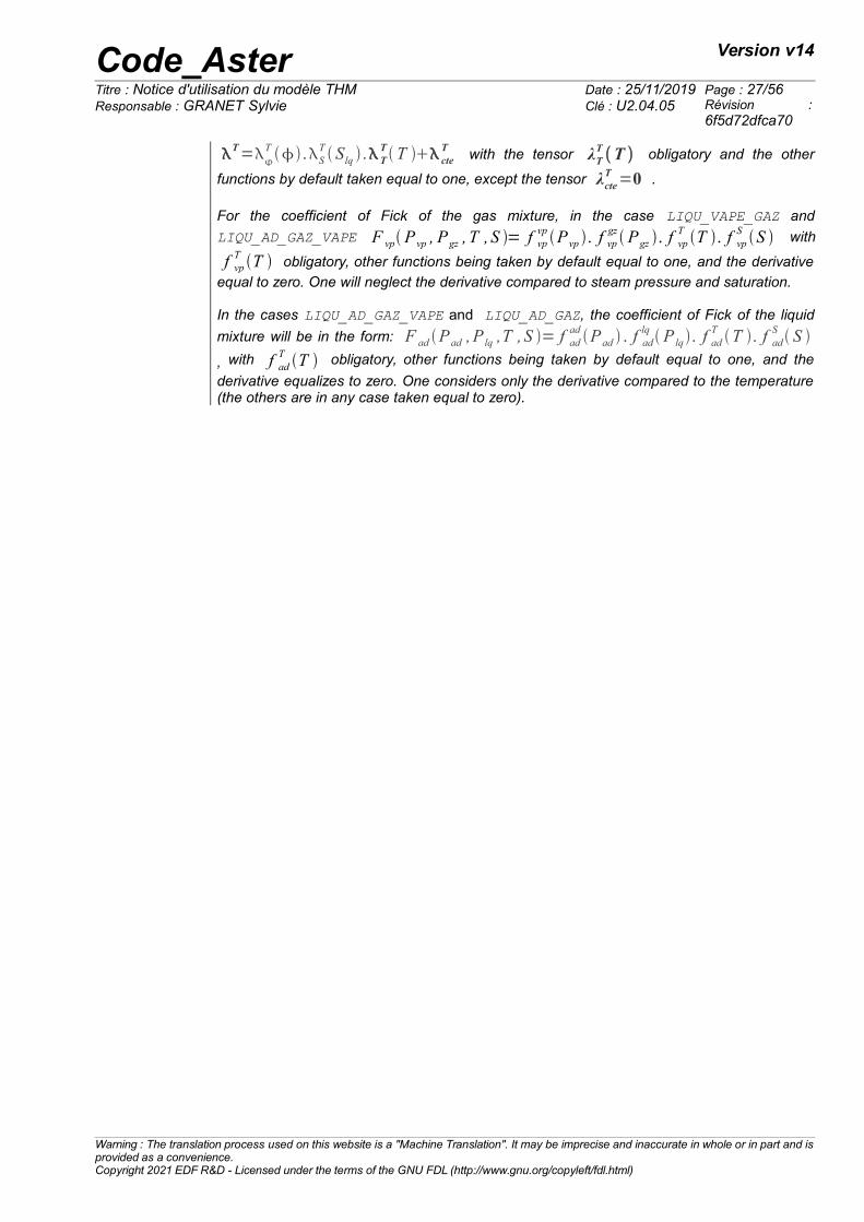
If there is thermics:
T is function of porosity, saturation and temperature and is given in the shape of theproduct of three functions:
Warning : The translation process used on this website is a "Machine Translation". It may be imprecise and inaccurate in whole or in part and isprovided as a convenience.Copyright 2021 EDF R&D - Licensed under the terms of the GNU FDL (http://www.gnu.org/copyleft/fdl.html)
Code_Aster Version v14
Titre : Notice d'utilisation du modèle THM Date : 25/11/2019 Page : 27/56Responsable : GRANET Sylvie Clé : U2.04.05 Révision :
6f5d72dfca70
T=
T .ST Slq . T
T T cteT
with the tensor λTT T obligatory and the other
functions by default taken equal to one, except the tensor λcteT =0 .
For the coefficient of Fick of the gas mixture, in the case LIQU_VAPE_GAZ and
LIQU_AD_GAZ_VAPE F vp P vp , Pgz , T , S = f vpvpPvp . f vp
gz Pgz . f vp
TT . f vp
SS with
f vpTT obligatory, other functions being taken by default equal to one, and the derivative
equal to zero. One will neglect the derivative compared to steam pressure and saturation. In the cases LIQU_AD_GAZ_VAPE and LIQU_AD_GAZ, the coefficient of Fick of the liquid
mixture will be in the form: F ad Pad ,P lq ,T , S = f adadPad . f ad
lq P lq. f ad
TT . f ad
S S
, with f adTT obligatory, other functions being taken by default equal to one, and the
derivative equalizes to zero. One considers only the derivative compared to the temperature(the others are in any case taken equal to zero).
Warning : The translation process used on this website is a "Machine Translation". It may be imprecise and inaccurate in whole or in part and isprovided as a convenience.Copyright 2021 EDF R&D - Licensed under the terms of the GNU FDL (http://www.gnu.org/copyleft/fdl.html)
Code_Aster Version v14
Titre : Notice d'utilisation du modèle THM Date : 25/11/2019 Page : 28/56Responsable : GRANET Sylvie Clé : U2.04.05 Révision :
6f5d72dfca70
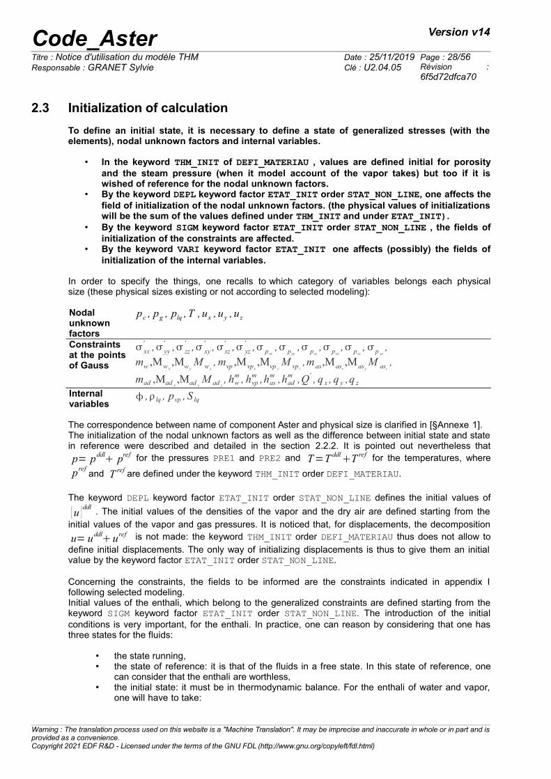
2.3 Initialization of calculation
To define an initial state, it is necessary to define a state of generalized stresses (with theelements), nodal unknown factors and internal variables.
• In the keyword THM_INIT of DEFI_MATERIAU , values are defined initial for porosityand the steam pressure (when it model account of the vapor takes) but too if it iswished of reference for the nodal unknown factors.
• By the keyword DEPL keyword factor ETAT_INIT order STAT_NON_LINE, one affects thefield of initialization of the nodal unknown factors. (the physical values of initializationswill be the sum of the values defined under THM_INIT and under ETAT_INIT).
• By the keyword SIGM keyword factor ETAT_INIT order STAT_NON_LINE , the fields ofinitialization of the constraints are affected.
• By the keyword VARI keyword factor ETAT_INIT one affects (possibly) the fields ofinitialization of the internal variables.
In order to specify the things, one recalls to which category of variables belongs each physicalsize (these physical sizes existing or not according to selected modeling):
Nodalunknownfactors
pc , pg , plq , T , ux , uy , uz
Constraintsat the pointsof Gauss
xx' , yy
' , zz' , xy
' , xz' , yz
' , pxx, pyy
, pzz, pxy
, pxz, p yz
,
mw ,Mw x,Mw y
M w z, mvp ,Mvpx
,Mvp yM vp z
,m as,Masx,Mas y
M asz,
mad ,Mad x,Mad y
M ad z, hw
m , hvpm ,has
m ,hadm ,Q' , q x , q y ,q z
Internalvariables
,lq , pvp , S lq
The correspondence between name of component Aster and physical size is clarified in [§Annexe 1].The initialization of the nodal unknown factors as well as the difference between initial state and statein reference were described and detailed in the section 2.2.2. It is pointed out nevertheless that
p= pddl pref for the pressures PRE1 and PRE2 and T=T ddl
T ref for the temperatures, where
prefand T ref are defined under the keyword THM_INIT order DEFI_MATERIAU.
The keyword DEPL keyword factor ETAT_INIT order STAT_NON_LINE defines the initial values of
{u }ddl
. The initial values of the densities of the vapor and the dry air are defined starting from the
initial values of the vapor and gas pressures. It is noticed that, for displacements, the decomposition
u= uddluref
is not made: the keyword THM_INIT order DEFI_MATERIAU thus does not allow to
define initial displacements. The only way of initializing displacements is thus to give them an initialvalue by the keyword factor ETAT_INIT order STAT_NON_LINE.
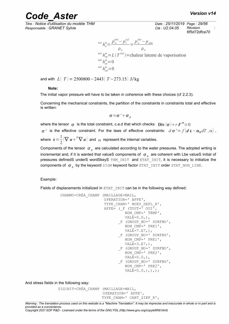
Concerning the constraints, the fields to be informed are the constraints indicated in appendix Ifollowing selected modeling.Initial values of the enthali, which belong to the generalized constraints are defined starting from thekeyword SIGM keyword factor ETAT_INIT order STAT_NON_LINE. The introduction of the initialconditions is very important, for the enthali. In practice, one can reason by considering that one hasthree states for the fluids:
• the state running,• the state of reference: it is that of the fluids in a free state. In this state of reference, one
can consider that the enthali are worthless,• the initial state: it must be in thermodynamic balance. For the enthali of water and vapor,
one will have to take:
Warning : The translation process used on this website is a "Machine Translation". It may be imprecise and inaccurate in whole or in part and isprovided as a convenience.Copyright 2021 EDF R&D - Licensed under the terms of the GNU FDL (http://www.gnu.org/copyleft/fdl.html)
Code_Aster Version v14
Titre : Notice d'utilisation du modèle THM Date : 25/11/2019 Page : 29/56Responsable : GRANET Sylvie Clé : U2.04.05 Révision :
6f5d72dfca70
init hwm=
pwinit− p l
ref
w
=pwinit−patm
winit hvp
m=L T init
=chaleur latente de vaporisationinit has
m=0
init hadm=0
and with L T = 2500800−2443 T−273.15 J / kg
Note:
The initial vapor pressure will have to be taken in coherence with these choices (cf 2.2.3).
Concerning the mechanical constraints, the partition of the constraints in constraints total and effectiveis written:
= ' p
where the tensor is the total constraint, c.a.d that which checks: Div r F m=0
' is the effective constraint. For the laws of effective constraints: d '= f d −0dT , ,
where =12
∇ u ∇ uT and represent the internal variables.
Components of the tensor p are calculated according to the water pressures. The adopted writing is
incremental and, if it is wanted that valueS components of p are coherent with Lbe valueS initial ofpressures definedS underS wordSkeyS THM_INIT and ETAT_INIT, it is necessary to initialize the
components of p by the keyword SIGM keyword factor ETAT_INIT order STAT_NON_LINE.
Example:
Fields of displacements initialized in ETAT_INIT can be in the following way defined:
CHAMNO=CRÉA_CHAMP (MAILLAGE=MAIL, OPERATION=' AFFE', TYPE_CHAM=' NOEU_DEPL_R', AFFE= (_F (TOUT=' OUI', NOM_CMP=' TEMP', VALE=0.0,), _F (GROUP_NO=' SURFBO', NOM_CMP=' PRE1', VALE=7.E7,), _F (GROUP_NO=' SURFBG', NOM_CMP=' PRE1', VALE=3.E7,), _F (GROUP_NO=' SURFBO', NOM_CMP=' PRE2', VALE=0.0,), _F (GROUP_NO=' SURFBG', NOM_CMP=' PRE2', VALE=0.0,),),);
And stress fields in the following way:
SIGINIT=CRÉA_CHAMP (MAILLAGE=MAIL, OPERATION=' AFFE', TYPE_CHAM=' CART_SIEF_R',
Warning : The translation process used on this website is a "Machine Translation". It may be imprecise and inaccurate in whole or in part and isprovided as a convenience.Copyright 2021 EDF R&D - Licensed under the terms of the GNU FDL (http://www.gnu.org/copyleft/fdl.html)
Code_Aster Version v14
Titre : Notice d'utilisation du modèle THM Date : 25/11/2019 Page : 30/56Responsable : GRANET Sylvie Clé : U2.04.05 Révision :
6f5d72dfca70
AFFE= (_F (GROUP_MA=' BO', NOM_CMP= (‘SIXX’, ‘SIYY’, ‘SIZZ’, ‘SIXY’, ‘SIXZ’, ‘SIYZ’, ‘SIPXX’, ‘SIPYY’, ‘SIPZZ’, ‘SIPXY’, ‘SIPXZ’, ‘SIPYZ’, ‘M11’, ‘FH11X’, ‘FH11Y’, ‘ENT11’, ‘M12’, ‘FH12X’, ‘FH12Y’, ‘ENT12’, ‘QPRIM’, ‘FHTX’, ‘FHTY’, ‘M21’, ‘FH21X’, ‘FH21Y’, ‘ENT21’, ‘M22’, ‘FH22X’, ‘FH22Y’, ‘ENT22’,), VALE= (0.0, 0.0, 0.0, 0.0, 0.0, 0.0,0.0, 0.0, 0.0, 0.0, 0.0,0.0, 0.0,0.0, 0.0, 0.0, 0.0,0.0, 0.0, 2500000.0, 0.0,0.0, 0.0, 0.0, 0.0, 0.0, 0.0, 0. , 0. , 0. , 0.),),),);
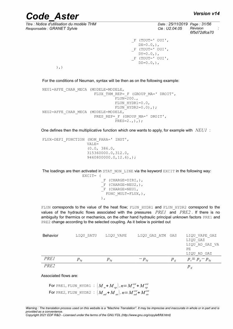
2.4 Loadings and boundary conditions
All the boundary conditions or loading are affected via the order AFFE_CHAR_MECA [U4.44.01]. Theloadings are then activated by the keyword factor EXCIT order STAT_NON_LINE.
In a classical way, three types of boundary conditions are possible:
• Conditions of the Dirichlet type which consist in imposing on part of border of the values fixed
for principal unknown factors belonging to {u }ddl
(and not u= uddluinit ) for that one uses
the keyword factor DDL_IMPO or FACE_IMPO of AFFE_CHAR_MECA.• Conditions of the Neumann type which consist in imposing values on the “dual quantities”,
either by not saying anything (worthless flows in hydraulics and thermics), or in their giving avalue via the keywords FLUN, FLUN_HYDR1 and FLUN_HYDR2 keyword factor FLUX_THM_REPorder AFFE_CHAR_MECA. This flow is then multiplied by a function of time (by defaultequalizes to 1) called by FONC_MULT under keyword EXCIT order STAT_NON_LINE. FLUN,FLUN_HYDR1 and FLUN_HYDR2 the heat fluxes, water flows and flows of gas componentrepresent respectively (cf, end of the paragraph).
• Conditions of the type mixed (or “of exchange”) who consist – in unsaturated - to impose an“external” condition for each principal unknown factor of hydraulics ( pc , pg ) as well as thecoefficients of corresponding exchange. In fine that consists in imposing a value on the “dualquantities” function of the external pressures and coefficients of exchange (in a linear way).The external pressures and the coefficients of exchanges are respectively indicated by thekeywords PRE1_EXT and PRE2_EXT and COEF_11, COEF_12, COEF_21, COEF_22, by usingthe keyword factor ECHANGE_THM order AFFE_CHAR_MECA.
• Mechanical conditions in total constraints .n are they given via PRES_REP orderAFFE_CHAR_MECA. One will refer to the documentation of this order to know the possibilitiesof them.
From a syntactic point of view the conditions of Dirichlet thus apply as to the following example
DIRI=AFFE_CHAR_MECA (MODELE=MODELE, DDL_IMPO= (_F (GROUP_NO=' GAUCHE', TEMP=0.0,), _F (TOUT=' OUI', PRE2=0.0,), _F (GROUP_NO=' GAUCHE', PRE1=0.0,),
Warning : The translation process used on this website is a "Machine Translation". It may be imprecise and inaccurate in whole or in part and isprovided as a convenience.Copyright 2021 EDF R&D - Licensed under the terms of the GNU FDL (http://www.gnu.org/copyleft/fdl.html)
Code_Aster Version v14
Titre : Notice d'utilisation du modèle THM Date : 25/11/2019 Page : 31/56Responsable : GRANET Sylvie Clé : U2.04.05 Révision :
6f5d72dfca70
_F (TOUT=' OUI', DX=0.0,), _F (TOUT=' OUI', DY=0.0,), _F (TOUT=' OUI', DZ=0.0,),),)
For the conditions of Neuman, syntax will be then as on the following example:
NEU1=AFFE_CHAR_MECA (MODELE=MODELE, FLUX_THM_REP=_F (GROUP_MA=' DROIT',
FLUN=200., FLUN_HYDR1=0.0, FLUN_HYDR2=0.0),);
NEU2=AFFE_CHAR_MECA (MODELE=MODELE, PRES_REP=_F (GROUP_MA=' DROIT',
PRES=2.,),);
One defines then the multiplicative function which one wants to apply, for example with NEU1 :
FLUX=DEFI_FONCTION (NOM_PARA=' INST', VALE= (0.0, 386.0, 315360000.0,312.0, 9460800000.0,12.6),);
The loadings are then activated in STAT_NON_LINE via the keyword EXCIT in the following way: EXCIT= ( _F (CHARGE=DIRI,), _F (CHARGE=NEU2,), _F (CHARGE=NEU1, FONC_MULT=FLUX,), ),
FLUN corresponds to the value of the heat flow; FLUN_HYDR1 and FLUN_HYDR2 correspond to thevalues of the hydraulic flows associated with the pressures PRE1 and PRE2 . If there is noambiguity for thermics or mechanics, on the other hand hydraulic principal unknown factors PRE1 andPRE2 change according to the selected coupling. As it below is pointed out
Behavior LIQU_SATU LIQU_VAPE LIQU_GAZ_ATM GAS LIQU_VAPE_GAZLIQU_GAZLIQU_AD_GAZ_VAPELIQU_AD_GAZ
PRE1 p lq p lq −p lq p g pc= pg− p lq
PRE2 p g
Associated flows are:
For PRE1, FLUN_HYDR1 : (M w+M vp ) .n=M wext+M vp
ext
For PRE2, FLUN_HYDR2 : (M ad+M as ). n=M adext+M as
ext
Warning : The translation process used on this website is a "Machine Translation". It may be imprecise and inaccurate in whole or in part and isprovided as a convenience.Copyright 2021 EDF R&D - Licensed under the terms of the GNU FDL (http://www.gnu.org/copyleft/fdl.html)
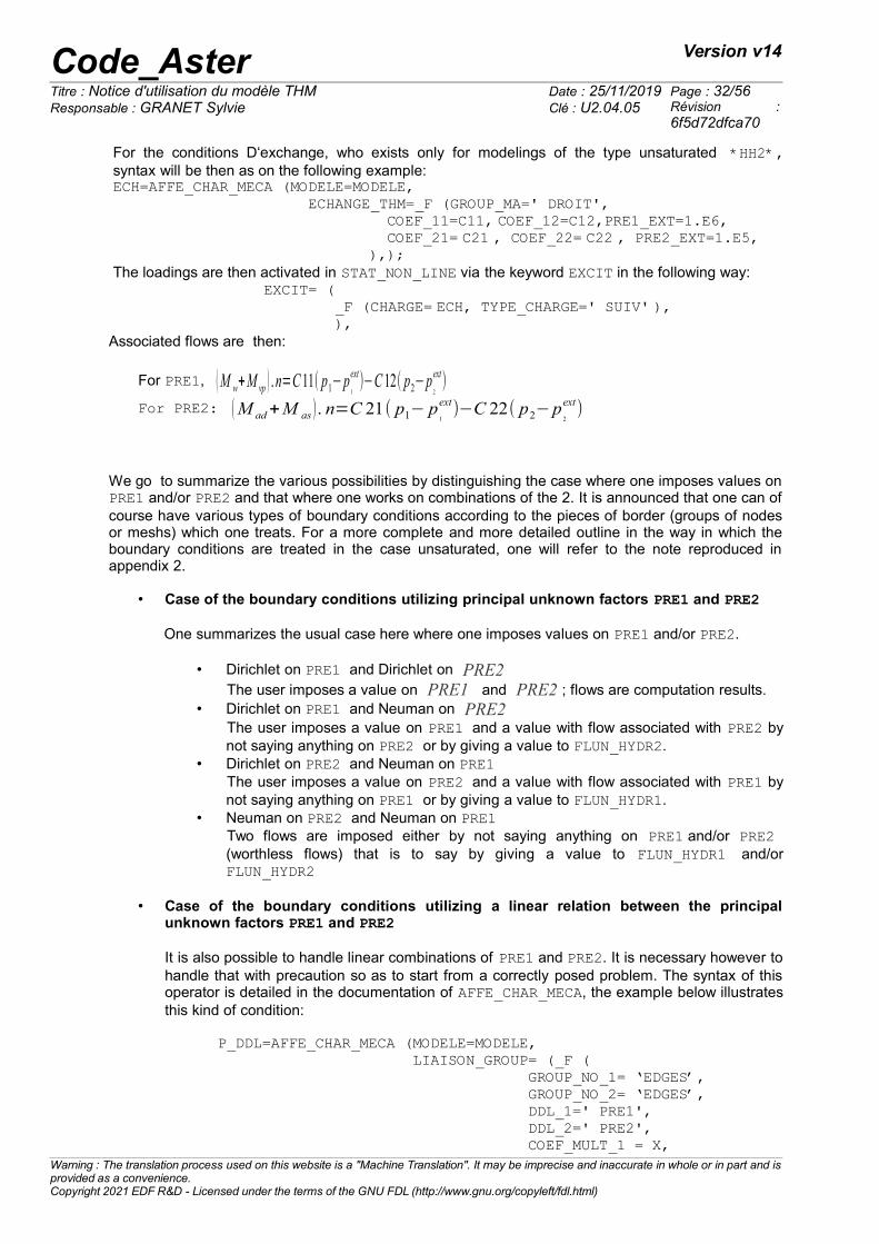
Code_Aster Version v14
Titre : Notice d'utilisation du modèle THM Date : 25/11/2019 Page : 32/56Responsable : GRANET Sylvie Clé : U2.04.05 Révision :
6f5d72dfca70
For the conditions D‘exchange, who exists only for modelings of the type unsaturated *HH2*,syntax will be then as on the following example:ECH=AFFE_CHAR_MECA (MODELE=MODELE, ECHANGE_THM=_F (GROUP_MA=' DROIT',
COEF_11=C11, COEF_12=C12,PRE1_EXT=1.E6, COEF_21= C21 , COEF_22= C22 , PRE2_EXT=1.E5, ),);
The loadings are then activated in STAT_NON_LINE via the keyword EXCIT in the following way: EXCIT= ( _F (CHARGE= ECH, TYPE_CHARGE=' SUIV' ), ),
Associated flows are then:
For PRE1, (M w+M vp ) .n=C11( p1− p1
ext)−C12( p2−p2
ext)
For PRE2: (M ad+M as ). n=C 21( p1− p1
ext)−C 22( p2−p2
ext)
We go to summarize the various possibilities by distinguishing the case where one imposes values onPRE1 and/or PRE2 and that where one works on combinations of the 2. It is announced that one can ofcourse have various types of boundary conditions according to the pieces of border (groups of nodesor meshs) which one treats. For a more complete and more detailed outline in the way in which theboundary conditions are treated in the case unsaturated, one will refer to the note reproduced inappendix 2.
• Case of the boundary conditions utilizing principal unknown factors PRE1 and PRE2
One summarizes the usual case here where one imposes values on PRE1 and/or PRE2.
• Dirichlet on PRE1 and Dirichlet on PRE2The user imposes a value on PRE1 and PRE2 ; flows are computation results.
• Dirichlet on PRE1 and Neuman on PRE2The user imposes a value on PRE1 and a value with flow associated with PRE2 bynot saying anything on PRE2 or by giving a value to FLUN_HYDR2.
• Dirichlet on PRE2 and Neuman on PRE1 The user imposes a value on PRE2 and a value with flow associated with PRE1 bynot saying anything on PRE1 or by giving a value to FLUN_HYDR1.
• Neuman on PRE2 and Neuman on PRE1Two flows are imposed either by not saying anything on PRE1 and/or PRE2 (worthless flows) that is to say by giving a value to FLUN_HYDR1 and/orFLUN_HYDR2
• Case of the boundary conditions utilizing a linear relation between the principalunknown factors PRE1 and PRE2
It is also possible to handle linear combinations of PRE1 and PRE2. It is necessary however tohandle that with precaution so as to start from a correctly posed problem. The syntax of thisoperator is detailed in the documentation of AFFE_CHAR_MECA, the example below illustratesthis kind of condition:
P_DDL=AFFE_CHAR_MECA (MODELE=MODELE, LIAISON_GROUP= (_F ( GROUP_NO_1= ‘EDGES’, GROUP_NO_2= ‘EDGES’, DDL_1=' PRE1', DDL_2=' PRE2', COEF_MULT_1 = X,
Warning : The translation process used on this website is a "Machine Translation". It may be imprecise and inaccurate in whole or in part and isprovided as a convenience.Copyright 2021 EDF R&D - Licensed under the terms of the GNU FDL (http://www.gnu.org/copyleft/fdl.html)
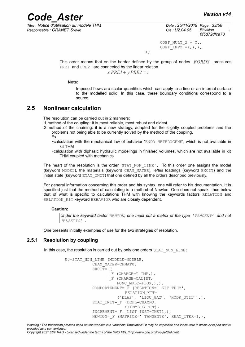
Code_Aster Version v14
Titre : Notice d'utilisation du modèle THM Date : 25/11/2019 Page : 33/56Responsable : GRANET Sylvie Clé : U2.04.05 Révision :
6f5d72dfca70
COEF_MULT_2 = Y., COEF_IMPO =z,),), );
This order means that on the border defined by the group of nodes BORDS , pressuresPRE1 and PRE2 are connected by the linear relation
x PRE1 y PRE2= z
Note:
Imposed flows are scalar quantities which can apply to a line or an internal surfaceto the modelled solid. In this case, these boundary conditions correspond to asource.
2.5 Nonlinear calculation
The resolution can be carried out in 2 manners:1.method of the coupling: it is most reliable, most robust and oldest2.method of the chaining: it is a new strategy, adapted for the slightly coupled problems and the
problems not being able to be currently solved by the method of the coupling.Ex: •calculation with the mechanical law of behavior ‘ENDO_HETEROGENE‘, which is not available in
kit THM•calculation with diphasic hydraulic modelings in finished volumes, which are not available in kit
THM coupled with mechanics
The heart of the resolution is the order ‘STAT_NON_LINE'. To this order one assigns the model(keyword MODEL), the materials (keyword CHAM_MATER), le/les loadings (keyword EXCIT) and theinitial state (keyword ETAT_INIT) that one defined by all the orders described previously.
For general information concerning this order and his syntax, one will refer to his documentation. It isspecified just that the method of calculating is a method of Newton. One does not speak thus belowthat of what is specific to calculations THM with knowing the keywords factors RELATION andRELATION_KIT keyword BEHAVIOR who are closely dependent.
Caution:
Under the keyword factor NEWTON, one must put a matrix of the type ‘TANGENT’ and not‘ELASTIC’ .
One presents initially examples of use for the two strategies of resolution.
2.5.1 Resolution by coupling
In this case, the resolution is carried out by only one orders STAT_NON_LINE:
U0=STAT_NON_LINE (MODELE=MODELE,CHAM_MATER=CHMAT0, EXCIT= (
_F (CHARGE=T_IMP,),_F (CHARGE=CALINT,
FONC_MULT=FLUX,),),COMPORTEMENT=_F (RELATION=' KIT_THHM',
RELATION_KIT=(‘ELAS’, ‘LIQU_GAZ’, ‘HYDR_UTIL’),),
ETAT_INIT=_F (DEPL=CHAMNO,SIGM=SIGINIT),
INCREMENT=_F (LIST_INST=INST1,),NEWTON=_F (MATRICE=' TANGENTE', REAC_ITER=1,),
Warning : The translation process used on this website is a "Machine Translation". It may be imprecise and inaccurate in whole or in part and isprovided as a convenience.Copyright 2021 EDF R&D - Licensed under the terms of the GNU FDL (http://www.gnu.org/copyleft/fdl.html)
Code_Aster Version v14
Titre : Notice d'utilisation du modèle THM Date : 25/11/2019 Page : 34/56Responsable : GRANET Sylvie Clé : U2.04.05 Révision :
6f5d72dfca70
CONVERGENCE=_F (RESI_GLOB_RELA=1.E-06,ITER_GLOB_MAXI=15,ITER_INTE_MAXI=5,),
ARCHIVAGE=_F (PAS_ARCH=1,),);
2.5.2 Resolution by chaining
The resolution by chaining currently applies to the only saturated Hydro-mechanical problems. Onepoints out initially the equations of this problem:
−∇⋅'ub∇ p=0
∂t∇⋅M lq=0
where porosity the law of behavior follows d=bd ∇⋅ub−
K s
dp .
Within the framework of the chaining, one solves separately the problems mechanics and hydraulics.The communication between two calculations is carried out via variables of order (‘PTOT’ and‘DIVU’). For the mechanical problem, the variable of order ‘PTOT’ play the part of the data ofpressure. For the hydraulic problem, the variable of order ‘DIVU’ play the part of the voluminal dataof deformation.These variables of order are calculated by the order CHAINAGE_THM.
The method illustrated below is a basic algorithm of pure chaining of calculations (hydraulic resolutionat moment 1, mechanical resolution at moment 1, hydraulic resolution at moment 2, mechanicalresolution at moment 2, etc…). One could consider more complicated algorithms (of type not fixes ornonlinear combined gradient) but that complexes of as much the setting in data in the command file.The question of the convergence of such algorithms is not either whole not acquired!The final mechanical solution is DEPLA and hydraulic solution is PRELIQ.
# buckles on the steps of timefor K in arranges (1, lenlinst):
UNPAS=DEFI_LISTE_REEL (DEBUT=listinst [k-1], INTERVALLE=_F (JUSQU_A=listinst [K],
NOMBRE=1,),);
UNPASSUB =DEFI_LISTE_INST (DEFI_LIST=_F (LIST_INST =UNPAS), ECHEC=_F ( SUBD_METHODE=' MANUEL', SUBD_PAS = 4, SUBD_NIVEAU=5,),);
yew (k>1):
DEFVHY=CHAINAGE_THM (RESULTAT=DEPLA, INFO=1, MODELE=MODHYD, MATR_PROJECTION=MATPROJ, TYPE_CHAINAGE=' MECA_HYDR', INST=listinst [K],);
MATEHY=AFFE_MATERIAU (MAILLAGE=MAIL, AFFE=_F (TOUT=' OUI', MATER=MATERIAU,), AFFE_VARC=_F (NOM_VARC=' DIVU',
Warning : The translation process used on this website is a "Machine Translation". It may be imprecise and inaccurate in whole or in part and isprovided as a convenience.Copyright 2021 EDF R&D - Licensed under the terms of the GNU FDL (http://www.gnu.org/copyleft/fdl.html)
Code_Aster Version v14
Titre : Notice d'utilisation du modèle THM Date : 25/11/2019 Page : 35/56Responsable : GRANET Sylvie Clé : U2.04.05 Révision :
6f5d72dfca70
EVOL=DEFVHY,),);
else:
MATEHY=AFFE_MATERIAU (MAILLAGE=MAIL, AFFE=_F (TOUT=' OUI', MATER=MATERIAU,),);
yew (k==1):
PRELIQ=STAT_NON_LINE (MODELE=MODHYD, CHAM_MATER=MATEHY, EXCIT=_F (CHARGE=CHARHYD,), SOLVEUR=_F (METHODE=' MUMPS', PCENT_PIVOT=100,), CONVERGENCE=_F (ITER_GLOB_MAXI=50,), ARCHIVAGE=_F (LIST_INST=UNPAS,), COMPORTEMENT=_F (RELATION=' KIT_H', RELATION_KIT= (‘LIQU_SATU’,‘HYDR_UTIL’,),), INCREMENT=_F (LIST_INST=UNPASSUB,),);
else:
PRELIQ=STAT_NON_LINE (reuse=PRELIQ, MODELE=MODHYD, CHAM_MATER=MATEHY, EXCIT=_F (CHARGE=CHARHYD,), SOLVEUR=_F (METHODE=' MUMPS', PCENT_PIVOT=100,), ARCHIVAGE=_F (LIST_INST=UNPAS,), ETAT_INIT=_F (EVOL_NOLI=PRELIQ, INST=listinst [k-1]), CONVERGENCE=_F (ITER_GLOB_MAXI=50,), COMPORTEMENT=_F (RELATION=' KIT_H', RELATION_KIT= (‘LIQU_SATU’,‘HYDR_UTIL’,),), INCREMENT=_F (LIST_INST=UNPASSUB,),);
yew (k>1):TO DESTROY (INFO=1, CONCEPT=_F (NOM= (REPTOT, MATEME,),),);
REPTOT=CHAINAGE_THM (RESULTAT=PRELIQ,
MODELE=MODMEC, TYPE_CHAINAGE=' HYDR_MECA', TYPE_RESU=' EVOL_VARC', INST=listinst [K],);
MATEME=AFFE_MATERIAU (MAILLAGE=MAIL, AFFE=_F (TOUT=' OUI', MATER=MATERIAU,), AFFE_VARC=_F (TOUT=' OUI', EVOL=REPTOT, NOM_VARC=' PTOT',),);
yew (k==1):
DEPLA=STAT_NON_LINE (MODELE=MODMEC, CHAM_MATER=MATEME, EXCIT=_F (CHARGE=CHARMEC,), COMPORTEMENT=_F (RELATION=' ELAS',),
Warning : The translation process used on this website is a "Machine Translation". It may be imprecise and inaccurate in whole or in part and isprovided as a convenience.Copyright 2021 EDF R&D - Licensed under the terms of the GNU FDL (http://www.gnu.org/copyleft/fdl.html)
Code_Aster Version v14
Titre : Notice d'utilisation du modèle THM Date : 25/11/2019 Page : 36/56Responsable : GRANET Sylvie Clé : U2.04.05 Révision :
6f5d72dfca70
INCREMENT=_F (LIST_INST=UNPASSUB,), ARCHIVAGE=_F (LIST_INST=UNPAS,), NEWTON=_F (MATRICE=' TANGENTE', REAC_ITER=10,), CONVERGENCE=_F (ITER_GLOB_MAXI=10,), SOLVEUR=_F (METHODE=' MUMPS',PCENT_PIVOT=100,),);
else:
DEPLA=STAT_NON_LINE (reuse=DEPLA, MODELE=MODMEC, CHAM_MATER=MATEME, EXCIT=_F (CHARGE=CHARMEC,), ARCHIVAGE=_F (LIST_INST=UNPAS,), COMPORTEMENT=_F (RELATION=' ELAS',), ETAT_INIT=_F (EVOL_NOLI=DEPLA, INST=listinst [k-1]), INCREMENT=_F (LIST_INST=UNPASSUB,), NEWTON=_F (MATRICE=' TANGENTE', REAC_ITER=10,), CONVERGENCE=_F (ITER_GLOB_MAXI=10,), SOLVEUR=_F (METHODE=' MUMPS',PCENT_PIVOT=100,),);
yew (k>1):TO DESTROY (INFO=1, CONCEPT=_F (NOM= (DEFVHY,),),);TO DESTROY (INFO=1, CONCEPT=_F (NOM= (UNPAS, UNPASSUB, MATEHY,),),);
2.5.3 General advices of use
RELATION is informed by relations of the types KIT_XXXX who allow to solve simultaneously from twoto four equilibrium equations. The equations considered depend on the suffix XXXX with the followingrule:
M indicate the mechanical equilibrium equation, T indicate the thermal equilibrium equation,H indicate a hydraulic equilibrium equation,V indicate the presence of a phase in form vapor (besides the liquid).
Only one letter H mean that the porous environment is saturated (only one variable with pressure p), for example either of gas, or of liquid, or of a liquid mixture/gas (of which the pressure of gas isconstant).Two letters H mean that the porous environment is not saturated (two variables with pressure p ),for example a liquid mixture/vapor/gas.The presence of the two letters HV mean that the porous environment is saturated by a component(in practice of water), but that this component can be in liquid form or vapor. There is not whereas anequation of conservation of this component, therefore only one degree of freedom pressure, but thereare a liquid flow and a flow vapor. The possible relations are then the following ones:
/ ‘KIT_HM’/ ‘KIT_THM’/ ‘KIT_HHM’/ ‘KIT_THH’/ ‘KIT_THV’/ ‘KIT_THHM’/ ‘KIT_HH’
Warning : The translation process used on this website is a "Machine Translation". It may be imprecise and inaccurate in whole or in part and isprovided as a convenience.Copyright 2021 EDF R&D - Licensed under the terms of the GNU FDL (http://www.gnu.org/copyleft/fdl.html)
Code_Aster Version v14
Titre : Notice d'utilisation du modèle THM Date : 25/11/2019 Page : 37/56Responsable : GRANET Sylvie Clé : U2.04.05 Révision :
6f5d72dfca70
The table below summarizes to which kit each modeling corresponds:
KIT_HM D_PLAN_HM, D_PLAN_HMD, D_PLAN_HMS, D_PLAN_HM_SI, AXIS_HM,AXIS_HMD, AXIS_HMS, 3D_HM, 3D_HMD, 3D_HMS, 3D_HM_SI
KIT_THM D_PLAN_THM, D_PLAN_THMD, D_PLAN_THMS, AXIS_THM, AXIS_THMD,AXIS_THMS, 3D_THM, 3D_THMD, 3D_THMS
KIT_HHM D_PLAN_HHM, D_PLAN_HHMD, D_PLAN_HHMS, AXIS_HHM, AXIS_HHMD,AXIS_HHMS, 3D_HHM, 3D_HHMD, 3D_HHMS, D_PLAN_HH2MD,AXIS_HH2MD, 3D_HH2MD, D_PLAN_HH2MS, AXIS_HH2MS, 3D_HH2MS,D_PLAN_HH2M_SI, 3D_HH2M_SI
KIT_THH D_PLAN_THHD, D_PLAN_THHS, AXIS_THHD, AXIS_THHS, 3D_THHD,3D_THHS, D_PLAN_THH2D, AXIS_THH2D, 3D_THH2D, D_PLAN_THH2S,AXIS_THH2S, 3D_THH2S
KIT_THV D_PLAN_THVD, AXIS_THVD, 3D_THVDKIT_THHM D_PLAN_THHMD, D_PLAN_THHMS, AXIS_THHMD, AXIS_THHMS, 3D_THHM,
3D_THHMD, 3D_THHMS, D_PLAN_THH2MD, AXIS_THH2MD, 3D_THH2MD,D_PLAN_THH2MS, AXIS_THH2MS, 3D_THH2MS
KIT_HH D_PLAN_HHD, AXIS_HHD, 3D_HHD, D_PLAN_HH2D, AXIS_HH2D,3D_HH2D,D_PLAN_HHS, AXIS_HHS, 3D_HHS, D_PLAN_HH2S, AXIS_HH2S,3D_HH2S
For each modelled phenomenon (hydraulic and/or mechanical), one must specify in RELATION_KIT :
• The mechanical model of behavior of the skeleton if there is mechanical modeling (M),
/ ‘ELAS’/ ‘MOHR_COULOMB’/ ‘CJS’/ ‘HUJEUX’/ ‘CAM_CLAY’/ ‘BARCELONA’/ ‘LAIGLE’/ ‘LETK’/ ‘DRUCK_PRAGER’/ ‘DRUCK_PRAG_N_A‘/ ‘VISC_DRUCK_PRAG’/ ‘GONF_ELAS‘/ ‘HOEK_BROWN_TOT’/ ‘HOEK_BROWN_EFF’/ ‘MAZARS’/ ‘ENDO_ISOT_BETON’
• The gas/liquid reaction of, (the same one as that indicated in COMP_THM underDEFI_MATERIAU, cf [§2.2.2])
/ ‘LIQU_SATU’/ ‘LIQU_GAZ’/ ‘GAS’/ ‘LIQU_GAZ_ATM’/ ‘LIQU_VAPE_GAZ’/ ‘LIQU_AD_GAZ_VAPE’/ ‘LIQU_AD_GAZ’/ ‘LIQU_VAPE’
Warning : The translation process used on this website is a "Machine Translation". It may be imprecise and inaccurate in whole or in part and isprovided as a convenience.Copyright 2021 EDF R&D - Licensed under the terms of the GNU FDL (http://www.gnu.org/copyleft/fdl.html)
Code_Aster Version v14
Titre : Notice d'utilisation du modèle THM Date : 25/11/2019 Page : 38/56Responsable : GRANET Sylvie Clé : U2.04.05 Révision :
6f5d72dfca70
• Concerning the hydraulic behavior, the user currently has 4 choices:
/ ‘HYDR_UTIL’/ ‘HYDR_ENDO’/ ‘HYDR_VGM’/ ‘HYDR_VGC’
• Either it chooses HYDR_UTIL : this keyword then makes it possible to inform the curveof saturation and its derivative according to the capillary pressure as well as therelative permeability and its derivative according to saturation. The user returnsthese curves via a series of formulas then called by DEFI_MATERIAU (cf 2.2.7).
• Either it chooses HYDR_ENDO : it is the same thing but allows the use of the laws withdamage ‘MAZARS‘and’ENDO_ISOT_BETON‘(the permeability is then coupled with thedamage).
• Either it chooses HYDR_VGM or HYDR_VGC what means that the laws of capillarity andpermeabilities will obey the model of preset Mualem-Van-Genuchten in the code, in otherwords, the capillarity is given by a law of Van Genuchten:
Swe=S−Swr
1−S wr
and m=1−1n
S we =1
[1+( Pc−Pe
P r)n
]m
The permeability relating to water is expressed then by integrating the model of predictionproposed by Mualem (1976) in the model of capillarity of Van-Genuchten:
k rw=S we 1−1−S we
1/m m
2
The permeability to gas is formulated in a similar way by a law of Parker for HYDR_VGM :
k rgz=1−S we 1−S we
1 /m 2m
or by a cubic law for HYDR_VGC:
k rgz=1−S 3
with in all the cases parameters n , Pr , Pe , Swr , Smax defined inDEFI_MATERIAU :
n corresponds to the parameter VG_NPr corresponds to the parameter VG_PR
• Pe corresponds to the parameter VG_P ENTR (0 by default)
Swr corresponds to the parameter VG_SR
With that must be added two additional parameters corresponding to a treatment whichone carries out on these curves:
Smax who corresponds to the parameter VG_SMAXCSAT who corresponds to the parameter VG_SATUR
We now will clarify what is this treatment and what are CSAT and Smax . ForSSmax , these curves are interpolated by a polynomial of degree 2, C1 in Smax , so
as to avoid having to treat derivative of infinite values. Indeed, for S=1 :Warning : The translation process used on this website is a "Machine Translation". It may be imprecise and inaccurate in whole or in part and isprovided as a convenience.Copyright 2021 EDF R&D - Licensed under the terms of the GNU FDL (http://www.gnu.org/copyleft/fdl.html)
Code_Aster Version v14
Titre : Notice d'utilisation du modèle THM Date : 25/11/2019 Page : 39/56Responsable : GRANET Sylvie Clé : U2.04.05 Révision :
6f5d72dfca70
∂ krwS
∂ S=∞
and in the case of HYDR_VGM:
∂ kr
gzS
∂ S=∞
To avoid having to deal with this problem (which does not have a priori physical meaning) onereplaces these functions starting from a saturation Smax by a polynomial of the second order C1 inthis point.
What gives for the function k rw S :
For S=Smax , the polynomial is determined PLS such as
{PLSmax =k r
wSmax
PL' Smax=∂ k r
w
∂ SS max
and PL1=0
For SSmax , k rw S is replaced by PLS .
And, in the case of HYDR_VGM, for k rgzS :
For S=Smax , the polynomial is determined PG S such as
{PG Smax=kr
gzSmax
PG ' Smax=∂ k r
gz
∂ SSmax
and PG 0=1
For SSmax , k rgzS is replaced by PG S like the example Figure 2.5.3-a. In the
case of a cubic law, no special treatment is necessary.
Warning : The translation process used on this website is a "Machine Translation". It may be imprecise and inaccurate in whole or in part and isprovided as a convenience.Copyright 2021 EDF R&D - Licensed under the terms of the GNU FDL (http://www.gnu.org/copyleft/fdl.html)
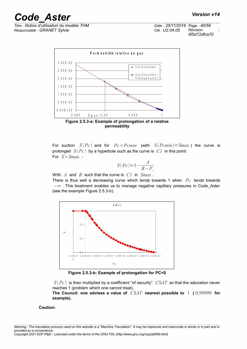
Code_Aster Version v14
Titre : Notice d'utilisation du modèle THM Date : 25/11/2019 Page : 40/56Responsable : GRANET Sylvie Clé : U2.04.05 Révision :
6f5d72dfca70
For suction S Pc and for PcPcmin (with S Pcmin=Smax ) the curve isprolonged S Pc by a hyperbole such as the curve is C1 in this point: For SSmax :
S Pc =1−A
B−P c
With A and B such that the curve is C1 in Smax . There is thus well a decreasing curve which tends towards 1 when Pc tends towards−∞ . This treatment enables us to manage negative capillary pressures in Code_Aster
(see the example Figure 2.5.3-b).
S Pc is then multiplied by a coefficient “of security” CSAT so that the saturation never
reaches 1 (problem which one cannot treat).The Council: one advises a value of CSAT nearest possible to 1 ( 0,99999 forexample).
Caution:
Warning : The translation process used on this website is a "Machine Translation". It may be imprecise and inaccurate in whole or in part and isprovided as a convenience.Copyright 2021 EDF R&D - Licensed under the terms of the GNU FDL (http://www.gnu.org/copyleft/fdl.html)
Figure 2.5.3-a: Example of prolongation of a relativepermeability
P e r m é a b i l i t é r e l a t i v e a u g a z
0 , 0 0 E + 0 0
5 , 0 0 E - 0 3
1 , 0 0 E - 0 2
1 , 5 0 E - 0 2
2 , 0 0 E - 0 2
2 , 5 0 E - 0 2
3 , 0 0 E - 0 2
0 , 9 8 5 0 , 9 9 0 , 9 9 5 1
V a n - G e n u c h t e n
V a n - G e n u c h t e n +P r o l o n g e m e n t C 1
S m a x =
P e r m é a b i l i t é r e l a t i v e a u g a z
0 , 0 0 E + 0 0
5 , 0 0 E - 0 3
1 , 0 0 E - 0 2
1 , 5 0 E - 0 2
2 , 0 0 E - 0 2
2 , 5 0 E - 0 2
3 , 0 0 E - 0 2
0 , 9 8 5 0 , 9 9 0 , 9 9 5 1
V a n - G e n u c h t e n
V a n - G e n u c h t e n +P r o l o n g e m e n t C 1
S m a x =
Figure 2.5.3-b: Example of prolongation for PC<0
S ( P c )
0 , 4
0 , 6
0 , 8
1
- 5 , 0 0 E + 06
0 , 0 0 E + 0 0 5 , 0 0 E + 0 6 1 , 0 0 E + 0 7 1 , 5 0 E + 0 7 2 , 0 0 E + 0 7 2 , 5 0 E + 0 7 3 , 0 0 E + 0 7
P c
S
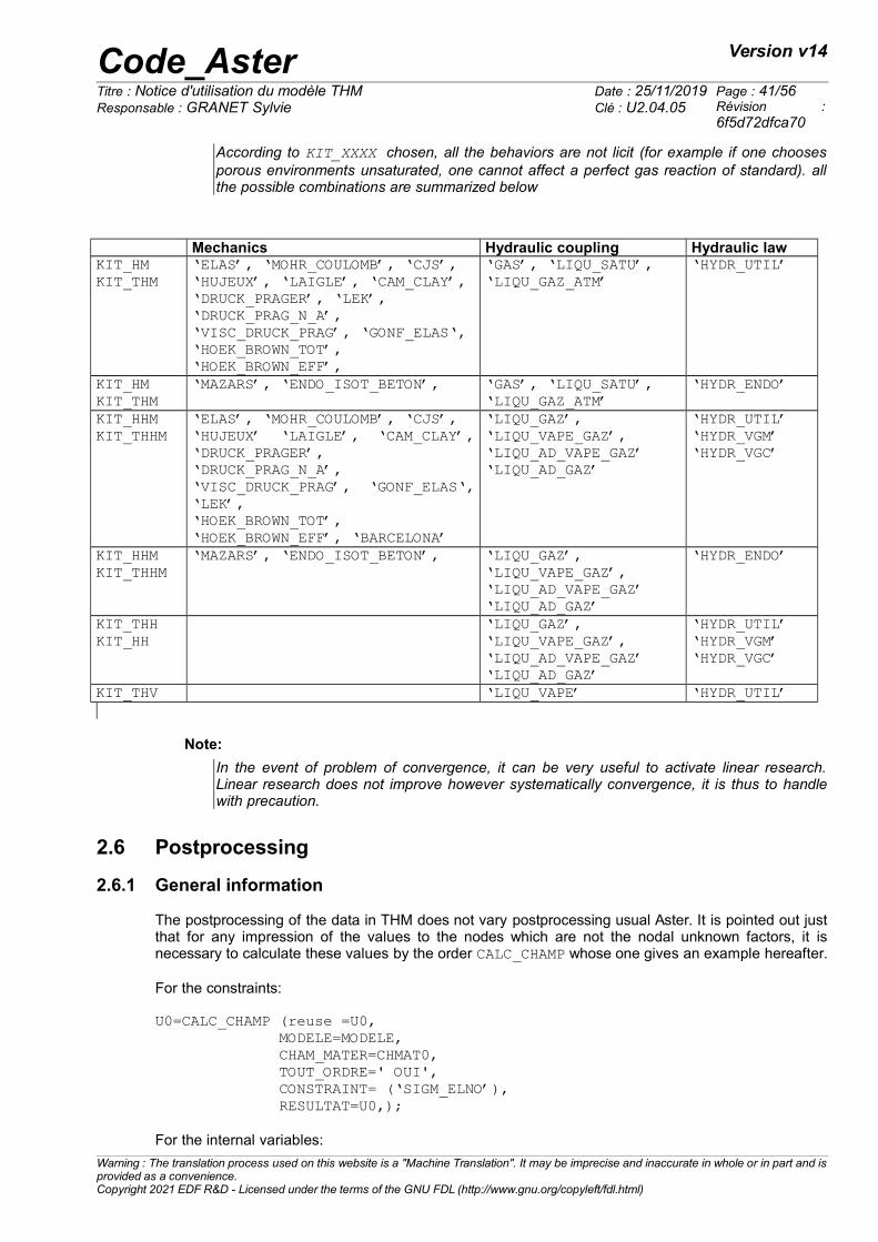
Code_Aster Version v14
Titre : Notice d'utilisation du modèle THM Date : 25/11/2019 Page : 41/56Responsable : GRANET Sylvie Clé : U2.04.05 Révision :
6f5d72dfca70
According to KIT_XXXX chosen, all the behaviors are not licit (for example if one choosesporous environments unsaturated, one cannot affect a perfect gas reaction of standard). allthe possible combinations are summarized below
Mechanics Hydraulic coupling Hydraulic lawKIT_HMKIT_THM
‘ELAS’, ‘MOHR_COULOMB’, ‘CJS’,‘HUJEUX’, ‘LAIGLE’, ‘CAM_CLAY’,‘DRUCK_PRAGER’, ‘LEK’,‘DRUCK_PRAG_N_A’,‘VISC_DRUCK_PRAG’, ‘GONF_ELAS‘,‘HOEK_BROWN_TOT’,‘HOEK_BROWN_EFF’,
‘GAS’, ‘LIQU_SATU’,‘LIQU_GAZ_ATM’
‘HYDR_UTIL’
KIT_HMKIT_THM
‘MAZARS’, ‘ENDO_ISOT_BETON’, ‘GAS’, ‘LIQU_SATU’,‘LIQU_GAZ_ATM’
‘HYDR_ENDO’
KIT_HHMKIT_THHM
‘ELAS’, ‘MOHR_COULOMB’, ‘CJS’,‘HUJEUX’ ‘LAIGLE’, ‘CAM_CLAY’,‘DRUCK_PRAGER’,‘DRUCK_PRAG_N_A’,‘VISC_DRUCK_PRAG’, ‘GONF_ELAS‘,‘LEK’,‘HOEK_BROWN_TOT’,‘HOEK_BROWN_EFF’, ‘BARCELONA’
‘LIQU_GAZ’,‘LIQU_VAPE_GAZ’,‘LIQU_AD_VAPE_GAZ’‘LIQU_AD_GAZ’
‘HYDR_UTIL’‘HYDR_VGM’‘HYDR_VGC’
KIT_HHMKIT_THHM
‘MAZARS’, ‘ENDO_ISOT_BETON’, ‘LIQU_GAZ’,‘LIQU_VAPE_GAZ’,‘LIQU_AD_VAPE_GAZ’‘LIQU_AD_GAZ’
‘HYDR_ENDO’
KIT_THHKIT_HH
‘LIQU_GAZ’,‘LIQU_VAPE_GAZ’,‘LIQU_AD_VAPE_GAZ’‘LIQU_AD_GAZ’
‘HYDR_UTIL’‘HYDR_VGM’‘HYDR_VGC’
KIT_THV ‘LIQU_VAPE’ ‘HYDR_UTIL’
Note:
In the event of problem of convergence, it can be very useful to activate linear research.Linear research does not improve however systematically convergence, it is thus to handlewith precaution.
2.6 Postprocessing
2.6.1 General information
The postprocessing of the data in THM does not vary postprocessing usual Aster. It is pointed out justthat for any impression of the values to the nodes which are not the nodal unknown factors, it isnecessary to calculate these values by the order CALC_CHAMP whose one gives an example hereafter.
For the constraints:
U0=CALC_CHAMP (reuse =U0, MODELE=MODELE, CHAM_MATER=CHMAT0, TOUT_ORDRE=' OUI', CONSTRAINT= (‘SIGM_ELNO’), RESULTAT=U0,);
For the internal variables:
Warning : The translation process used on this website is a "Machine Translation". It may be imprecise and inaccurate in whole or in part and isprovided as a convenience.Copyright 2021 EDF R&D - Licensed under the terms of the GNU FDL (http://www.gnu.org/copyleft/fdl.html)
Code_Aster Version v14
Titre : Notice d'utilisation du modèle THM Date : 25/11/2019 Page : 42/56Responsable : GRANET Sylvie Clé : U2.04.05 Révision :
6f5d72dfca70
U0=CALC_CHAMP (reuse =U0, MODELE=MODELE, CHAM_MATER=CHMAT0, TOUT_ORDRE=' OUI', VARI_INTERNE= (‘VARI_ELNO’), RESULTAT=U0,);
It should however be recalled that all the values of displacements at exits correspond to uddl and not
u=uddluref
.
It is also important to know the name of the constraints and the numbers of the internal variables. Allthat is consigned in appendix I.Thus the following example makes it possible to print the liquid water mass on the group of nodesHAUT at every moment.
TAB1=POST_RELEVE_T (ACTION=_F (INTITULE=' CONT', GROUP_NO= (‘HIGH’), RESULTAT=U0, NOM_CHAM=' SIEF_ELNO', TOUT_ORDRE=' OUI', NOM_CMP= (‘M11’), OPERATION=' EXTRACTION',),);
IMPR_TABLE (TABLE=TAB1, FICHIER=' RESULTAT', FORMAT=' AGRAF', PAGINATION=' INST', NOM_PARA= (‘INST’, ‘COOR_X’, ‘M11’),);
The following example makes it possible to print the values of porosity to node 1 and the first moment.
TAB2=POST_RELEVE_T (ACTION=_F (INTITULE=' DEPL', NOEUD=' NO1', RESULTAT=U0, NOM_CHAM=' VARI_ELNO', NUME_ORDRE=1, NOM_CMP= (‘V2’), OPERATION=' EXTRACTION',),);IMPR_TABLE (TABLE=TAB2, FICHIER=' RESULTAT', FORMAT=' AGRAF', PAGINATION=' INST', NOM_PARA= (‘INST’, ‘COOR_X’, ‘V2’),);
2.6.2 Internal variables
In addition to the general information suggested above, there exists from now on a means moreconvivial D '' of extracting the internal variables (cf Doc. U4.81.01). For that of the fields were createdfrom which the principle is to extract from the field VARI_ELGA (or VARI_ELNO for fields calculatedwith the nodes) the internal variable which interests us via a keyword more speaking that V1 , V2 ,…
As a postprocessing these fields are calculated by CALC_CHAMP. Syntax to be used is the followingone:
• for a field with the elements cham_elem
Warning : The translation process used on this website is a "Machine Translation". It may be imprecise and inaccurate in whole or in part and isprovided as a convenience.Copyright 2021 EDF R&D - Licensed under the terms of the GNU FDL (http://www.gnu.org/copyleft/fdl.html)
Code_Aster Version v14
Titre : Notice d'utilisation du modèle THM Date : 25/11/2019 Page : 43/56Responsable : GRANET Sylvie Clé : U2.04.05 Révision :
6f5d72dfca70
GAMP=CALC_CHAMP (RESULTAT=U0,OPTION=' VAEX_ELNO',NOM_VARI=' GAMP');
• for a field with the nodes cham_no :
GAMP=CALC_CHAMP (reuse=GAMP,RESULTAT=GAMP,VARI_INTERNE=' VAEX_NOEU');
Since it is just a question of extracting one (and only one!!) variable intern, them cham_elemcorrespondents must be calculated as a preliminary:U0=CALC_CHAMP (reuse =U0, MODELE=MODELE, CHAM_MATER=CHMAT0, TOUT_ORDRE=' OUI', VARI_INTERNE= (‘VARI_ELNO’), RESULTAT=U0,);
The list of the various reference symbols of the internal variables is:
“DPORO” variation of the porosity of material“DRHOLQ” variation of the density of material“DPVP” variation of the steam pressure“SATLIQ” saturation of the liquid“EVP” cumulated voluminal plastic deformation“IND_ETA” Mechanical indicator of state“D” Value of the damage“IND_END” Indicator of damage“TEMP_MAX” Maximum temperature“GAMP” Plastic deformation déviatoire cumulated“PCR” Critical pressure“SEUIL_HYD” Hydrous threshold“IND_HYD” Hydrous indicator of irreversibility“PCOHE” Pressure of cohesion“COMP_ROC” Behavior of the rock“SEUIL_ISO” Isotropic threshold“ANG_DEV” Angle of the threshold déviatoire“X11” Components of the kinematic tensor of work hardening“X22” Components of the kinematic tensor of work hardening“X33” Components of the kinematic tensor of work hardening“X12” Components of the kinematic tensor of work hardening“X13” Components of the kinematic tensor of work hardening“X23” Components of the kinematic tensor of work hardening“DIST_DEV” Distance standardized with the threshold déviatoire“DEV_SUR_CRIT” Relationship between the threshold déviatoire and the critical
threshold deviatoric“DIST_ISO” Distance standardized with the isotropic threshold“NB_ITER” Iteration count internal“STOP” Value of the local test of stop of the iterative process“NB_REDE” Number of local recutting of the step of time“SIGN” Sign of the contracted product of the deviatoric constraint by
the deviatoric plastic deformation
Note:
When the variable to be extracted is not part of the internal variables of the laws concerned,an alarm is emitted but the field is affected all the same with R8VIDE ().
Warning : The translation process used on this website is a "Machine Translation". It may be imprecise and inaccurate in whole or in part and isprovided as a convenience.Copyright 2021 EDF R&D - Licensed under the terms of the GNU FDL (http://www.gnu.org/copyleft/fdl.html)
Code_Aster Version v14
Titre : Notice d'utilisation du modèle THM Date : 25/11/2019 Page : 44/56Responsable : GRANET Sylvie Clé : U2.04.05 Révision :
6f5d72dfca70
2.6.3 Isovaleurs
Caution: linear distinction resolution and quadratic grid
One recalls that for any problem THM and in order to avoid any ambiguity for the user, the grid used isalways quadratic. On the other hand the resolution of the hydraulic and thermal problem is linear:unknown factors PRE1 , PRE2 and TEMP thus exist only on the nodes tops of the grid.
At the conclusion of calculation, one gets a result in this form:•Pressures PRE1 , PRE2 and temperatures TEMP are on the nodes tops of the elements.•The internal variables, the constraints are on the points of gauss and/or the nodes of the quadratic
grid (according to whether one into selective or in is lumpé) and displacements mechanical are onthe tops and the nodes mediums.
There is thus a conflict between the quadratic grids and linear calculations what will pose a problemfor example to trace isovaleurs.
There then exists a manner simple to be freed from this problem by projecting the whole of the resultson the linear grid resulting from the quadratic grid. Thus all the results will be defined at the sameplace (on the tops). For TEMP , PRE1 and PRE2 , it is enough to project as on the following example:
## projection of the quadratic grid on the linear grid:
MAILQ4 = CREA_MAILLAGE ( GRID = E-MAIL, QUAD_LINE = _F (ALL = ‘YES’), )
## assignment of the model corresponding:
MODELQ4=AFFE_MODELE (MAILLAGE=MAILQ4, AFFE=_F (TOUT=' OUI', PHENOMENE=' MECANIQUE', MODELISATION=' D_PLAN',),);
## projection of the result on this new model:
RESULIN = PROJ_CHAMP ( METHODE=' ELEM', RESULTAT=resu, MODELE_1=MODELQ8, MODELE_2=MODELQ4, NOM_CHAM = ' DEPL', TOUT_ORDRE=' OUI')
## usual postprocessing but on the linear grid:
IMPR_RESU (FORMAT=' MED', RESU=_F ( RESULTAT=RESULIN, NUME_ORDRE= (1,10,20,),
NOM_CMP = (‘PRE1’, ‘PRE2’,), MAILLAGE=MAILQ4,),);
Warning : The translation process used on this website is a "Machine Translation". It may be imprecise and inaccurate in whole or in part and isprovided as a convenience.Copyright 2021 EDF R&D - Licensed under the terms of the GNU FDL (http://www.gnu.org/copyleft/fdl.html)
Code_Aster Version v14
Titre : Notice d'utilisation du modèle THM Date : 25/11/2019 Page : 45/56Responsable : GRANET Sylvie Clé : U2.04.05 Révision :
6f5d72dfca70
There exists an alternative method, which can prove faster for the large industrial studies. Thismethod uses MACR_ADAP_MAIL. It is supposed that resu is composed of nbinst momentsstored in the list linst. Preceding postprocessing can also be done in the following way:
PRE = [Nun] *nbinst;PREB = [Nun] *nbinst; for K in arranges (nbinst): PRE [K] =CRÉA_CHAMP (TYPE_CHAM=' NOEU_DEPL_R', OPERATION=' EXTR', RESULTAT=resu, NOM_CHAM=' DEPL', INST=linst [K],);
motcle1= {}motcle2= {}
motcle1 [‘MAJ_CHAM’] = []motcle2 [‘AFFE’] = []
for K in arranges (nbinst):
PREB [K] =CO (‘PREB_%d' % (K)) motcle1 [‘MAJ_CHAM’] .append ( _F (TYPE_CHAM=' NOEU_DEPL_R', CHAM_GD = PRE [K], CHAM_MAJ = PREB [K],),);
motcle2 [‘AFFE’] .append ( _F (CHAM_GD=PREB [K], INST=linst [K],),);
MACR_ADAP_MAIL (ADAPTATION=' MODIFICATION', DEGRE=' OUI', MAILLAGE_N = MAILQ8, MAILLAGE_NP1 = CO (‘MAILQ4’), ** motcle1);
RESULINB=CRÉA_RESU (OPERATION=' AFFE', TYPE_RESU=' EVOL_NOLI', NOM_CHAM='DEPL', ** motcle2);
2.7 Some cases tests
On a purely informative basis, one recapitulates here some cases tests available in the base of Code_Aster.This list is absolutely not exhaustive but gives access directly a certain number of representative examples.
Name ofCAS-test
Type of modelingTHM
Phenomenonrepresented
Geometricalmodeling
Mixing rate
Wtna109a AXIS_THVD Désaturation byheating of a mediumwithout air
axisymmetric LIQU_VAPE
Wtna110a AXIS_HH2MS Modeling of a swellingof a clay
axisymmetric LIQU_AD_GAZ_VAPE
Wtna107 AXIS_THMS Heating of a mediumsaturated (THM)
axisymmetric LIQU_SATU
wtna112 AXIS_THMS Thermalpressurization of adrained test-tube
axisymmetric LIQU_SATU
Wtnp117a D_PLAN_HHS Capillary rebalancingof 2 materials
plane LIQU_GAZ
Warning : The translation process used on this website is a "Machine Translation". It may be imprecise and inaccurate in whole or in part and isprovided as a convenience.Copyright 2021 EDF R&D - Licensed under the terms of the GNU FDL (http://www.gnu.org/copyleft/fdl.html)
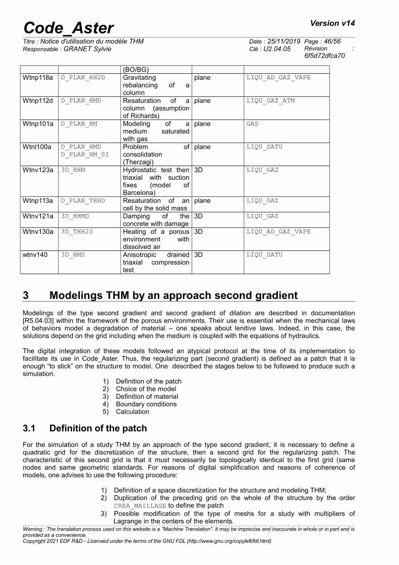
Code_Aster Version v14
Titre : Notice d'utilisation du modèle THM Date : 25/11/2019 Page : 46/56Responsable : GRANET Sylvie Clé : U2.04.05 Révision :
6f5d72dfca70
(BO/BG)Wtnp118a D_PLAN_HH2D Gravitating
rebalancing of acolumn
plane LIQU_AD_GAZ_VAPE
Wtnp112d D_PLAN_HMD Resaturation of acolumn (assumptionof Richards)
plane LIQU_GAZ_ATM
Wtnp101a D_PLAN_HM Modeling of amedium saturatedwith gas
plane GAS
Wtnl100a D_PLAN_HMDD_PLAN_HM_SI
Problem ofconsolidation(Therzagi)
plane LIQU_SATU
Wtnv123a 3D_HHM Hydrostatic test thentriaxial with suctionfixes (model ofBarcelona)
3D LIQU_GAZ
Wtnp113a D_PLAN_THHD Resaturation of ancell by the solid mass
plane LIQU_GAZ
Wtnv121a 3D_HHMD Damping of theconcrete with damage
3D LIQU_GAZ
Wtnv130a 3D_THH2S Heating of a porousenvironment withdissolved air
3D LIQU_AD_GAZ_VAPE
wtnv140 3D_HMS Anisotropic drainedtriaxial compressiontest
3D LIQU_SATU
3 Modelings THM by an approach second gradient
Modelings of the type second gradient and second gradient of dilation are described in documentation[R5.04.03] within the framework of the porous environments. Their use is essential when the mechanical lawsof behaviors model a degradation of material – one speaks about lenitive laws. Indeed, in this case, thesolutions depend on the grid including when the medium is coupled with the equations of hydraulics.
The digital integration of these models followed an atypical protocol at the time of its implementation tofacilitate its use in Code_Aster. Thus, the regularizing part (second gradient) is defined as a patch that it isenough “to stick” on the structure to model. One described the stages below to be followed to produce such asimulation.
1) Definition of the patch2) Choice of the model3) Definition of material4) Boundary conditions5) Calculation
3.1 Definition of the patch
For the simulation of a study THM by an approach of the type second gradient, it is necessary to define aquadratic grid for the discretization of the structure, then a second grid for the regularizing patch. Thecharacteristic of this second grid is that it must necessarily be topologically identical to the first grid (samenodes and same geometric standards. For reasons of digital simplification and reasons of coherence ofmodels, one advises to use the following procedure:
1) Definition of a space discretization for the structure and modeling THM;2) Duplication of the preceding grid on the whole of the structure by the order
CREA_MAILLAGE to define the patch3) Possible modification of the type of meshs for a study with multipliers of
Lagrange in the centers of the elements.Warning : The translation process used on this website is a "Machine Translation". It may be imprecise and inaccurate in whole or in part and isprovided as a convenience.Copyright 2021 EDF R&D - Licensed under the terms of the GNU FDL (http://www.gnu.org/copyleft/fdl.html)
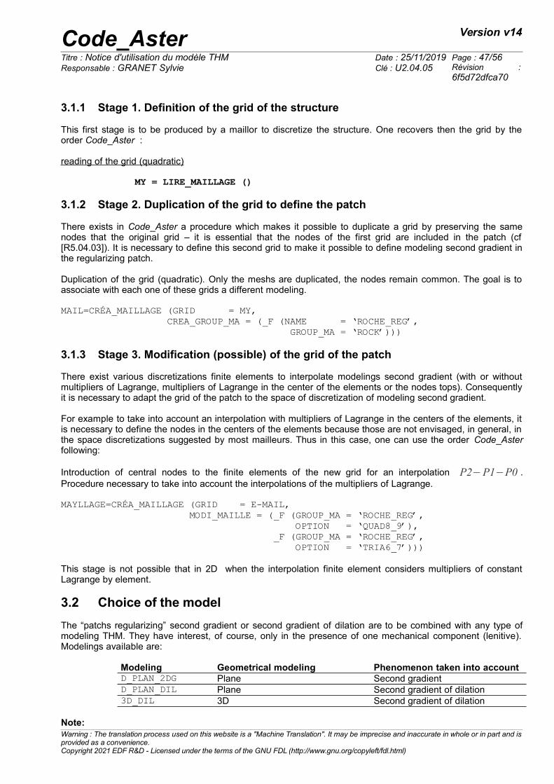
Code_Aster Version v14
Titre : Notice d'utilisation du modèle THM Date : 25/11/2019 Page : 47/56Responsable : GRANET Sylvie Clé : U2.04.05 Révision :
6f5d72dfca70
3.1.1 Stage 1. Definition of the grid of the structure This first stage is to be produced by a maillor to discretize the structure. One recovers then the grid by theorder Code_Aster :
reading of the grid (quadratic)
MY = LIRE_MAILLAGE ()
3.1.2 Stage 2. Duplication of the grid to define the patch There exists in Code_Aster a procedure which makes it possible to duplicate a grid by preserving the samenodes that the original grid – it is essential that the nodes of the first grid are included in the patch (cf[R5.04.03]). It is necessary to define this second grid to make it possible to define modeling second gradient inthe regularizing patch. Duplication of the grid (quadratic). Only the meshs are duplicated, the nodes remain common. The goal is toassociate with each one of these grids a different modeling.
MAIL=CRÉA_MAILLAGE (GRID = MY, CREA_GROUP_MA = (_F (NAME = ‘ROCHE_REG’, GROUP_MA = ‘ROCK’)))
3.1.3 Stage 3. Modification (possible) of the grid of the patch
There exist various discretizations finite elements to interpolate modelings second gradient (with or withoutmultipliers of Lagrange, multipliers of Lagrange in the center of the elements or the nodes tops). Consequentlyit is necessary to adapt the grid of the patch to the space of discretization of modeling second gradient.
For example to take into account an interpolation with multipliers of Lagrange in the centers of the elements, itis necessary to define the nodes in the centers of the elements because those are not envisaged, in general, inthe space discretizations suggested by most mailleurs. Thus in this case, one can use the order Code_Asterfollowing:
Introduction of central nodes to the finite elements of the new grid for an interpolation P2−P1−P0 .Procedure necessary to take into account the interpolations of the multipliers of Lagrange.
MAYLLAGE=CRÉA_MAILLAGE (GRID = E-MAIL, MODI_MAILLE = (_F (GROUP_MA = ‘ROCHE_REG’, OPTION = ‘QUAD8_9’), _F (GROUP_MA = ‘ROCHE_REG’, OPTION = ‘TRIA6_7’)))
This stage is not possible that in 2D when the interpolation finite element considers multipliers of constantLagrange by element.
3.2 Choice of the model The “patchs regularizing” second gradient or second gradient of dilation are to be combined with any type ofmodeling THM. They have interest, of course, only in the presence of one mechanical component (lenitive).Modelings available are:
Modeling Geometrical modeling Phenomenon taken into accountD_PLAN_2DG Plane Second gradientD_PLAN_DIL Plane Second gradient of dilation3D_DIL 3D Second gradient of dilation
Note:Warning : The translation process used on this website is a "Machine Translation". It may be imprecise and inaccurate in whole or in part and isprovided as a convenience.Copyright 2021 EDF R&D - Licensed under the terms of the GNU FDL (http://www.gnu.org/copyleft/fdl.html)
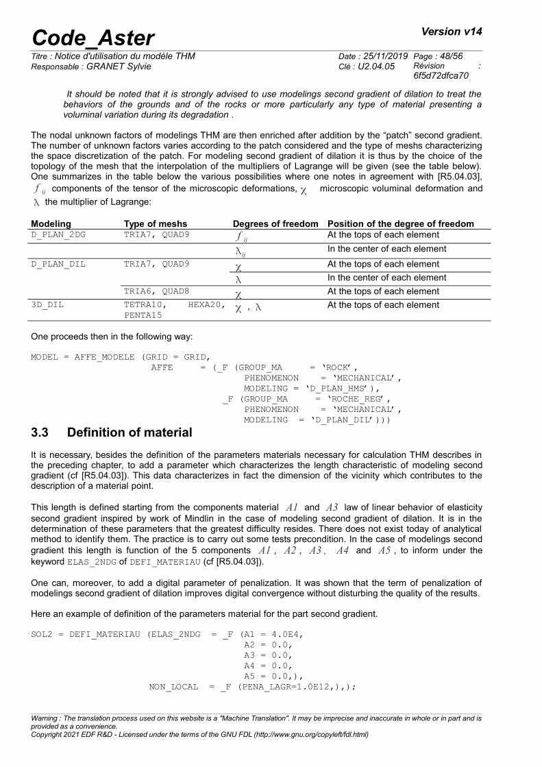
Code_Aster Version v14
Titre : Notice d'utilisation du modèle THM Date : 25/11/2019 Page : 48/56Responsable : GRANET Sylvie Clé : U2.04.05 Révision :
6f5d72dfca70
It should be noted that it is strongly advised to use modelings second gradient of dilation to treat thebehaviors of the grounds and of the rocks or more particularly any type of material presenting avoluminal variation during its degradation .
The nodal unknown factors of modelings THM are then enriched after addition by the “patch” second gradient.The number of unknown factors varies according to the patch considered and the type of meshs characterizingthe space discretization of the patch. For modeling second gradient of dilation it is thus by the choice of thetopology of the mesh that the interpolation of the multipliers of Lagrange will be given (see the table below).One summarizes in the table below the various possibilities where one notes in agreement with [R5.04.03],f ij components of the tensor of the microscopic deformations, microscopic voluminal deformation and
the multiplier of Lagrange:
Modeling Type of meshs Degrees of freedom Position of the degree of freedomD_PLAN_2DG TRIA7, QUAD9 f ij At the tops of each element
ij In the center of each element
D_PLAN_DIL TRIA7, QUAD9 At the tops of each element
In the center of each element
TRIA6, QUAD8 At the tops of each element
3D_DIL TETRA10, HEXA20,PENTA15
, At the tops of each element
One proceeds then in the following way:
MODEL = AFFE_MODELE (GRID = GRID, AFFE = (_F (GROUP_MA = ‘ROCK’, PHENOMENON = ‘MECHANICAL’, MODELING = ‘D_PLAN_HMS’), _F (GROUP_MA = ‘ROCHE_REG’, PHENOMENON = ‘MECHANICAL’, MODELING = ‘D_PLAN_DIL’)))
3.3 Definition of material
It is necessary, besides the definition of the parameters materials necessary for calculation THM describes inthe preceding chapter, to add a parameter which characterizes the length characteristic of modeling secondgradient (cf [R5.04.03]). This data characterizes in fact the dimension of the vicinity which contributes to thedescription of a material point.
This length is defined starting from the components material A1 and A3 law of linear behavior of elasticitysecond gradient inspired by work of Mindlin in the case of modeling second gradient of dilation. It is in thedetermination of these parameters that the greatest difficulty resides. There does not exist today of analyticalmethod to identify them. The practice is to carry out some tests precondition. In the case of modelings secondgradient this length is function of the 5 components A1 , A2 , A3 , A4 and A5 , to inform under thekeyword ELAS_2NDG of DEFI_MATERIAU (cf [R5.04.03]).
One can, moreover, to add a digital parameter of penalization. It was shown that the term of penalization ofmodelings second gradient of dilation improves digital convergence without disturbing the quality of the results.
Here an example of definition of the parameters material for the part second gradient. SOL2 = DEFI_MATERIAU (ELAS_2NDG = _F (A1 = 4.0E4, A2 = 0.0, A3 = 0.0, A4 = 0.0, A5 = 0.0,),
NON_LOCAL = _F (PENA_LAGR=1.0E12,),);
Warning : The translation process used on this website is a "Machine Translation". It may be imprecise and inaccurate in whole or in part and isprovided as a convenience.Copyright 2021 EDF R&D - Licensed under the terms of the GNU FDL (http://www.gnu.org/copyleft/fdl.html)
Code_Aster Version v14
Titre : Notice d'utilisation du modèle THM Date : 25/11/2019 Page : 49/56Responsable : GRANET Sylvie Clé : U2.04.05 Révision :
6f5d72dfca70
Then assignment of the parameters materials according to the same procedure as for the definition ofmodelings.
= AFFE_MATERIAU (GRID SUBDUE = GRID, AFFE = (_F (ALL = ‘ROCK’, MATER = SOL_HM,),
_F (GROUP_MA = ‘ROCHE_REG’, MATER = SOL2)))
3.4 Impact on the boundary conditions
There is no impact to bring in the command file Code_Aster to take into account the boundary conditions withmodelings second gradient compared to classical modelings THM. On the other hand, it is essential to note thatthe physical significance of the boundary conditions of pressure of normal constraints is modified withmodelings second gradient (cf [R5.04.03]).
3.5 Resolution DU problem
Calculation is to be carried out by the order STAT_NON_LINE. It is enough to add to classical calculation THMthe relation of behavior of elasticity second gradient on the grid corresponds to the patch as on the examplebelow (keyword ELAS). There is no incompatibility with the laws of behavior. To note, all the same, that asimulation THM by an approach second gradient has interest only in the presence of one mechanicalcomponent in coupled calculation.
It is important to note that when modeling takes into account an interpolation of the constant multipliers ofLagrange by elements it is necessary to use the solvor Mumps for the resolution.
Definition of nonlinear static calculation with a law of behavior associated with each one of modeling: behaviorof the Drucker-Prager type for the first gradient, and linear elasticity for the second gradient U1 = STAT_NON_LINE (MODEL = MODEL, CHAM_MATER = SUBDUE, EXCIT = (_F (LOAD = CHCI),…), SOLVEUR = (_F (METHODE=' MUMPS',)), BEHAVIOR = (_F (GROUP_MA=' ROCHE', RELATION = ‘DRUCK_PRAGER’,), _F (GROUP_MA = ‘ROCHE_REG’, RELATION = ‘ELAS’,),), NEWTON = _F (MATRIX = ‘TANGENT’, REAC_ITER = 1), INCREMENT = _F (LIST_INST = TIME))
One will find an example of modeling by second gradient, for example in the case test ssll117.
Warning : The translation process used on this website is a "Machine Translation". It may be imprecise and inaccurate in whole or in part and isprovided as a convenience.Copyright 2021 EDF R&D - Licensed under the terms of the GNU FDL (http://www.gnu.org/copyleft/fdl.html)
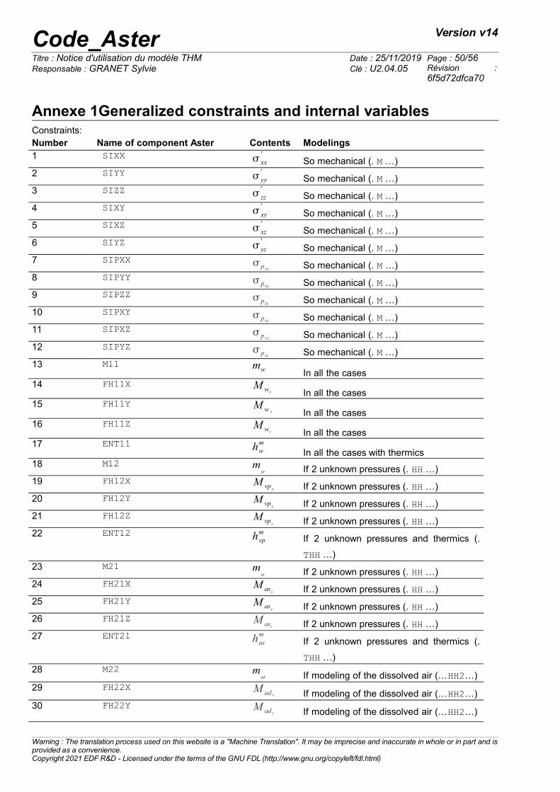
Code_Aster Version v14
Titre : Notice d'utilisation du modèle THM Date : 25/11/2019 Page : 50/56Responsable : GRANET Sylvie Clé : U2.04.05 Révision :
6f5d72dfca70
Annexe 1Generalized constraints and internal variablesConstraints: Number Name of component Aster Contents Modelings1 SIXX xx
' So mechanical (.
M
…)
2 SIYY yy'
So mechanical (. M
…)
3 SIZZ zz'
So mechanical (. M
…)
4 SIXY xy'
So mechanical (. M
…)
5 SIXZ xz'
So mechanical (. M
…)
6 SIYZ yz'
So mechanical (. M
…)
7 SIPXX pxx So mechanical (.
M
…)
8 SIPYY pyy So mechanical (.
M …)
9 SIPZZ pzz So mechanical (.
M
…)
10 SIPXY pxy So mechanical (.
M …)
11 SIPXZ pxz So mechanical (.
M
…)
12 SIPYZ pyz So mechanical (.
M …)
13 M11 mw In all the cases
14 FH11X M wx
In all the cases15 FH11Y M w y
In all the cases
16 FH11Z M wz
In all the cases17 ENT11 hw
m In all the cases with thermics
18 M12 mvp
If 2 unknown pressures (. HH
…)
19 FH12X M vp x If 2 unknown pressures (.
HH
…)
20 FH12Y M vpy If 2 unknown pressures (.
HH …)
21 FH12Z M vp z If 2 unknown pressures (.
HH
…)
22 ENT12 hvpm If 2 unknown pressures and thermics (.
THH …)
23 M21 mas
If 2 unknown pressures (. HH
…)
24 FH21X M asx If 2 unknown pressures (.
HH
…)
25 FH21Y M asy If 2 unknown pressures (. HH
…)
26 FH21Z M asz If 2 unknown pressures (. HH
…)
27 ENT21 hasm
If 2 unknown pressures and thermics (.
THH …)
28 M22 mad
If modeling of the dissolved air (…HH2…)29 FH22X M ad x
If modeling of the dissolved air (…HH2…)30 FH22Y M ad y
If modeling of the dissolved air (…HH2…)
Warning : The translation process used on this website is a "Machine Translation". It may be imprecise and inaccurate in whole or in part and isprovided as a convenience.Copyright 2021 EDF R&D - Licensed under the terms of the GNU FDL (http://www.gnu.org/copyleft/fdl.html)
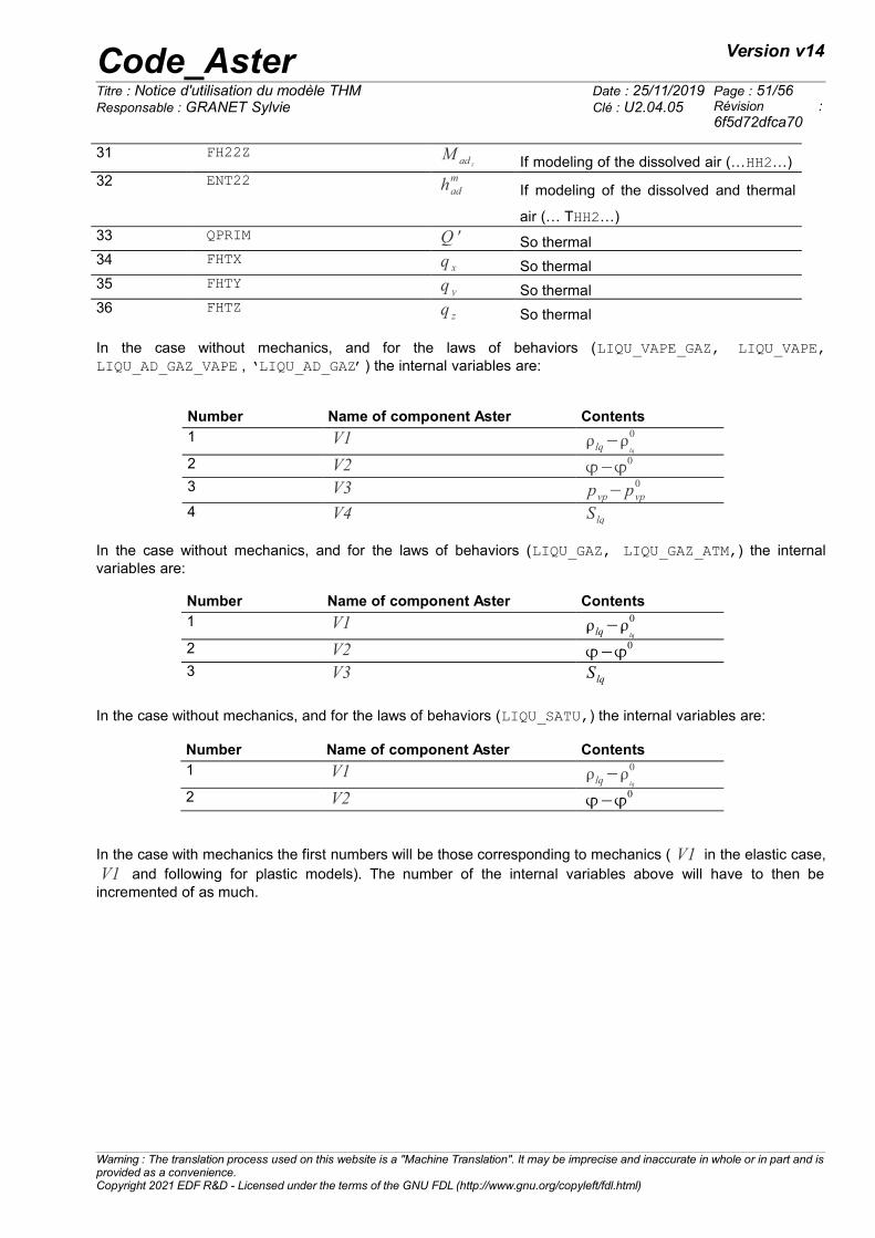
Code_Aster Version v14
Titre : Notice d'utilisation du modèle THM Date : 25/11/2019 Page : 51/56Responsable : GRANET Sylvie Clé : U2.04.05 Révision :
6f5d72dfca70
31 FH22Z M ad z If modeling of the dissolved air (…HH2…)
32 ENT22 hadm
If modeling of the dissolved and thermal
air (… THH2…)33 QPRIM Q ' So thermal34 FHTX q x So thermal35 FHTY q y So thermal36 FHTZ q z So thermal
In the case without mechanics, and for the laws of behaviors (LIQU_VAPE_GAZ, LIQU_VAPE,LIQU_AD_GAZ_VAPE , ‘LIQU_AD_GAZ’) the internal variables are:
Number Name of component Aster Contents1 V1 lq−
lq
0
2 V2 −0
3 V3 pvp−pvp0
4 V4 S lq
In the case without mechanics, and for the laws of behaviors (LIQU_GAZ, LIQU_GAZ_ATM,) the internalvariables are:
Number Name of component Aster Contents1 V1 lq−
lq
0
2 V2 −0
3 V3 S lq
In the case without mechanics, and for the laws of behaviors (LIQU_SATU,) the internal variables are:
Number Name of component Aster Contents1 V1 lq−
lq
0
2 V2 −0
In the case with mechanics the first numbers will be those corresponding to mechanics ( V1 in the elastic case,V1 and following for plastic models). The number of the internal variables above will have to then be
incremented of as much.
Warning : The translation process used on this website is a "Machine Translation". It may be imprecise and inaccurate in whole or in part and isprovided as a convenience.Copyright 2021 EDF R&D - Licensed under the terms of the GNU FDL (http://www.gnu.org/copyleft/fdl.html)
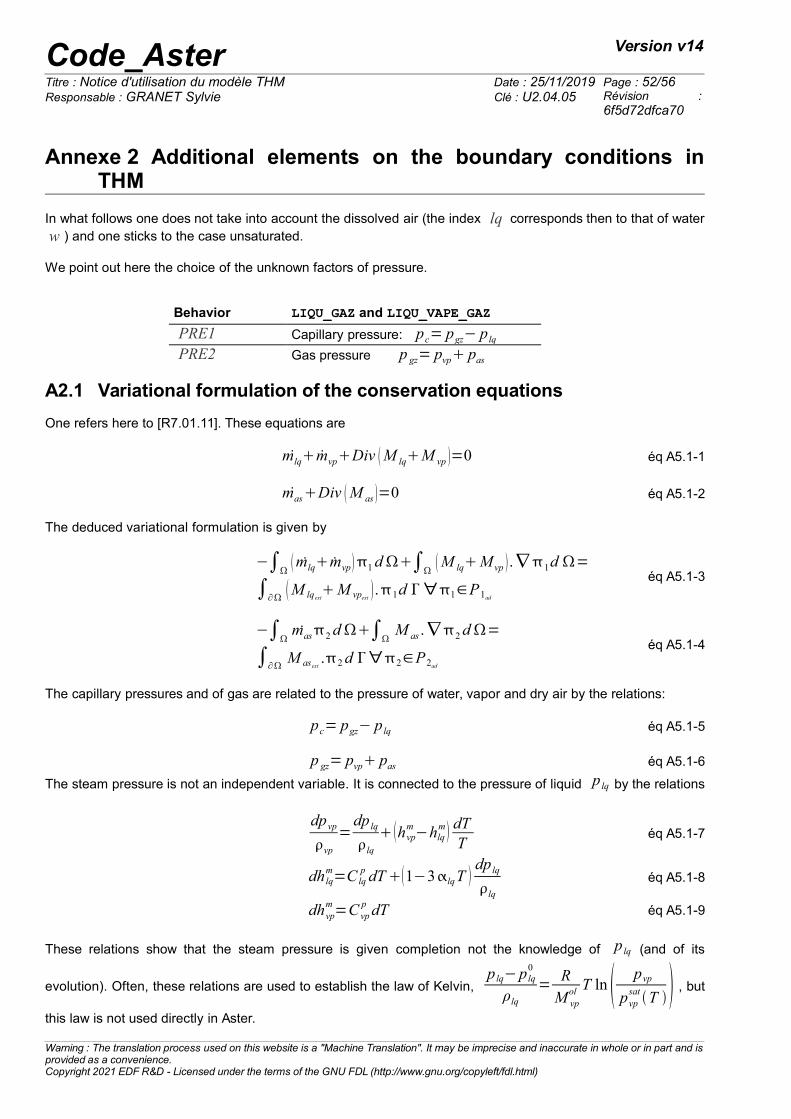
Code_Aster Version v14
Titre : Notice d'utilisation du modèle THM Date : 25/11/2019 Page : 52/56Responsable : GRANET Sylvie Clé : U2.04.05 Révision :
6f5d72dfca70
Annexe 2 Additional elements on the boundary conditions inTHM
In what follows one does not take into account the dissolved air (the index lq corresponds then to that of waterw ) and one sticks to the case unsaturated.
We point out here the choice of the unknown factors of pressure.
Behavior LIQU_GAZ and LIQU_VAPE_GAZ
PRE1 Capillary pressure: pc= pgz− p lq
PRE2 Gas pressure p gz= pvp pas
A2.1 Variational formulation of the conservation equations
One refers here to [R7.01.11]. These equations are
mlqmvpDiv M lqM vp =0 éq A5.1-1
masDiv M as =0 éq A5.1-2
The deduced variational formulation is given by
−∫ mlqmvp 1d∫
M lqM vp .∇1d =
∫∂ M lqextM vpext .1d ∀1∈P1ad
éq A5.1-3
−∫mas2d∫
M as . ∇2d=
∫∂M asext .2d ∀2∈P2ad
éq A5.1-4
The capillary pressures and of gas are related to the pressure of water, vapor and dry air by the relations:
pc= pgz− p lq éq A5.1-5
p gz= pvp pas éq A5.1-6
The steam pressure is not an independent variable. It is connected to the pressure of liquid p lq by the relations
dpvp
vp
=dp lq
lq
hvpm−hlq
m dTT
éq A5.1-7
dh lqm=C lq
p dT1−3lqT dp lq
lq
éq A5.1-8
dhvpm=C vp
p dT éq A5.1-9
These relations show that the steam pressure is given completion not the knowledge of p lq (and of its
evolution). Often, these relations are used to establish the law of Kelvin, p lq−p lq
0
ρlq
=RM vp
ol T ln pvp
pvpsatT , but
this law is not used directly in Aster. Warning : The translation process used on this website is a "Machine Translation". It may be imprecise and inaccurate in whole or in part and isprovided as a convenience.Copyright 2021 EDF R&D - Licensed under the terms of the GNU FDL (http://www.gnu.org/copyleft/fdl.html)
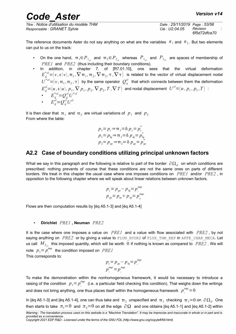
Code_Aster Version v14
Titre : Notice d'utilisation du modèle THM Date : 25/11/2019 Page : 53/56Responsable : GRANET Sylvie Clé : U2.04.05 Révision :
6f5d72dfca70
The reference documents Aster do not say anything on what are the variables π 1 and π 2 . But two elements
can put to us on the track:
• On the one hand, 1∈P1ad and 2∈P2ad
whereas P1ad and P2ad
are spaces of membership of
PRE1 and PRE2 (thus including their boundary conditions).• In addition, in chapter 7. of [R7.01.10], one sees that the virtual deformation
E g*el=v , v ,1 ,∇1 ,2 ,∇2 , ,∇ is related to the vector of virtual displacement nodal
U *el=v ,1 ,2 , by the same operator Q g
el that which connects between them the deformation
E gel= u , u , p1 ,∇ p1 , p2 ,∇ p2 , T ,∇ T and nodal displacement U el
=u , p1 , p2 ,T :
• E g*el=Q g
elU * el
• E gel=Q g
elU el
It is then clear that 1 and 2 are virtual variations of p1 and p2
From where the table:
p1= pc⇒1= pc= pc*
p1= plq⇒1= p lq= plq*
p2= pgz⇒2= pgz= pgz*
A2.2 Case of boundary conditions utilizing principal unknown factors
What we say in this paragraph and the following is relative to part of the border ∂d on which conditions areprescribed: nothing prevents of course that these conditions are not the same ones on parts of differentborders. We treat in this chapter the usual case where one imposes conditions on PRE1 and/or PRE2 , inopposition to the following chapter where we will speak about linear relations between unknown factors.
pc= pgz− p lq=pc
imp
p gz= pas pvp= pgz
imp
Flows are then computation results by [éq A5.1-3] and [éq A5.1-4]
• Dirichlet PRE1 , Neuman PRE2
It is the case where one imposes a value on PRE1 and a value with flow associated with PRE2 , by notsaying anything on PRE2 or by giving a value to FLUN_HYDR2 of FLUX_THM_REP in AFFE_CHAR_MECA. Let
us call M 2ext this imposed quantity, which will be worth 0 if nothing is known as compared to PRE2 . We will
note p1= p1
imp the condition imposed on PRE1
This corresponds to:
pc= pgz− p lq=pc
imp
p1
imp=p
c
imp
To make the demonstration within the nonhomogeneous framework, it would be necessary to introduce a
raising of the condition p1= p1
imp (i.e. a particular field checking this condition). That weighs down the writings
and does not bring anything, one thus places itself within the homogeneous framework p1
imp=0
In [éq A5.1-3] and [éq A5.1-4], one can thus take and 2 unspecified and 1 checking 1=0 on ∂d One
then starts to take π1=0 and π2=0 on all the edge ∂Ω and one obtains [éq A5.1-1] and [éq A5.1-2] within
Warning : The translation process used on this website is a "Machine Translation". It may be imprecise and inaccurate in whole or in part and isprovided as a convenience.Copyright 2021 EDF R&D - Licensed under the terms of the GNU FDL (http://www.gnu.org/copyleft/fdl.html)
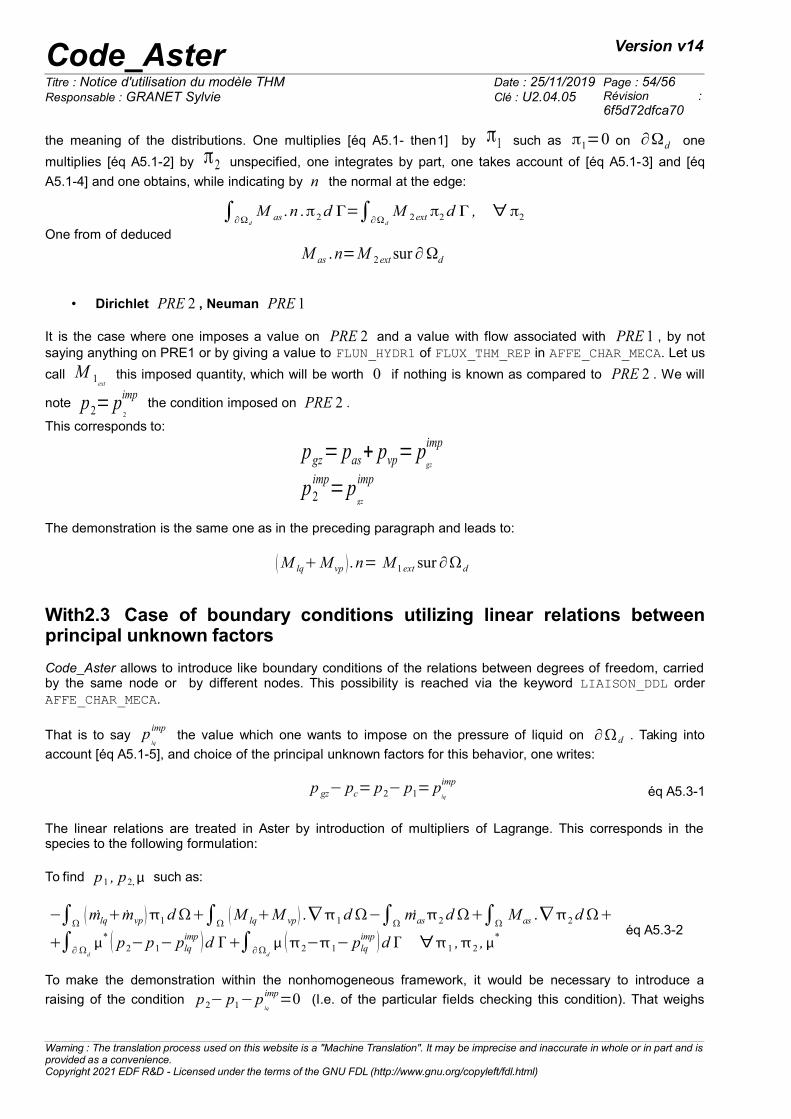
Code_Aster Version v14
Titre : Notice d'utilisation du modèle THM Date : 25/11/2019 Page : 54/56Responsable : GRANET Sylvie Clé : U2.04.05 Révision :
6f5d72dfca70
the meaning of the distributions. One multiplies [éq A5.1- then1] by π1 such as π1=0 on ∂Ωd one
multiplies [éq A5.1-2] by π2 unspecified, one integrates by part, one takes account of [éq A5.1-3] and [éq
A5.1-4] and one obtains, while indicating by n the normal at the edge:
∫∂Ωd
M as .n .π2d Γ=∫∂Ωd
M 2ext π2d Γ , ∀π2
One from of deduced
M as .n=M 2 ext sur ∂Ωd
• Dirichlet PRE 2 , Neuman PRE 1
It is the case where one imposes a value on PRE 2 and a value with flow associated with PRE 1 , by notsaying anything on PRE1 or by giving a value to FLUN_HYDR1 of FLUX_THM_REP in AFFE_CHAR_MECA. Let us
call M 1ext this imposed quantity, which will be worth 0 if nothing is known as compared to PRE 2 . We will
note p2= p2
imp the condition imposed on PRE 2 .
This corresponds to:
pgz= pas+ pvp= pgz
imp
p2imp=p
gz
imp
The demonstration is the same one as in the preceding paragraph and leads to:
M lqM vp .n= M 1ext sur ∂d
With2.3 Case of boundary conditions utilizing linear relations betweenprincipal unknown factors
Code_Aster allows to introduce like boundary conditions of the relations between degrees of freedom, carriedby the same node or by different nodes. This possibility is reached via the keyword LIAISON_DDL orderAFFE_CHAR_MECA.
That is to say plq
imp the value which one wants to impose on the pressure of liquid on ∂d . Taking into
account [éq A5.1-5], and choice of the principal unknown factors for this behavior, one writes:
p gz− pc= p2− p1= plq
impéq A5.3-1
The linear relations are treated in Aster by introduction of multipliers of Lagrange. This corresponds in thespecies to the following formulation: To find p1 , p2, such as:
−∫ mlqmvp 1d∫
M lqM vp .∇1d−∫mas2d∫
M as .∇2d
∫∂d
* p2−p1− plq
imp d ∫∂d
2−1− plqimp d ∀1 ,2 ,
* éq A5.3-2
To make the demonstration within the nonhomogeneous framework, it would be necessary to introduce a
raising of the condition p2− p1−plq
imp=0 (I.e. of the particular fields checking this condition). That weighs
Warning : The translation process used on this website is a "Machine Translation". It may be imprecise and inaccurate in whole or in part and isprovided as a convenience.Copyright 2021 EDF R&D - Licensed under the terms of the GNU FDL (http://www.gnu.org/copyleft/fdl.html)
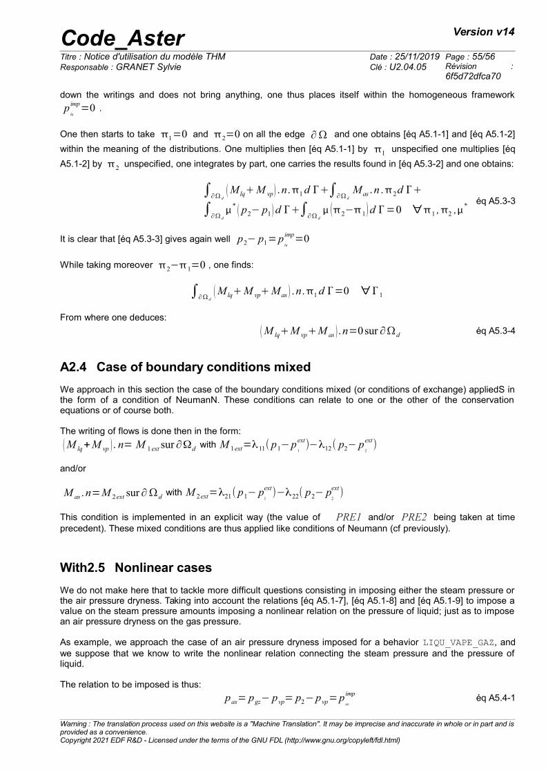
Code_Aster Version v14
Titre : Notice d'utilisation du modèle THM Date : 25/11/2019 Page : 55/56Responsable : GRANET Sylvie Clé : U2.04.05 Révision :
6f5d72dfca70
down the writings and does not bring anything, one thus places itself within the homogeneous framework
plq
imp=0 .
One then starts to take 1=0 and 2=0 on all the edge ∂ and one obtains [éq A5.1-1] and [éq A5.1-2]
within the meaning of the distributions. One multiplies then [éq A5.1-1] by 1 unspecified one multiplies [éq
A5.1-2] by 2 unspecified, one integrates by part, one carries the results found in [éq A5.3-2] and one obtains:
∫∂ dM lqM vp .n.1d ∫∂ d
M as .n .2d
∫∂ d
* p2− p1 d ∫
∂ d
2−1 d =0 ∀1 ,2 ,* éq A5.3-3
It is clear that [éq A5.3-3] gives again well p2− p1=plq
imp=0
While taking moreover 2−1=0 , one finds:
∫∂ dM lqM vpM as .n.1d =0 ∀1
From where one deduces:
M lqM vpM as .n=0sur ∂d éq A5.3-4
A2.4 Case of boundary conditions mixed
We approach in this section the case of the boundary conditions mixed (or conditions of exchange) appliedS inthe form of a condition of NeumanN. These conditions can relate to one or the other of the conservationequations or of course both.
The writing of flows is done then in the form:
(M lq+M vp ). n= M 1ext sur∂Ωd with M 1ext=λ11( p1−p1
ext)−λ12( p2− p
2
ext)
and/or
M as .n=M 2ext sur∂d with M 2ext=λ21( p1− p1
ext)−λ22( p2− p
2
ext)
This condition is implemented in an explicit way (the value of PRE1 and/or PRE2 being taken at timeprecedent). These mixed conditions are thus applied like conditions of Neumann (cf previously).
With2.5 Nonlinear cases
We do not make here that to tackle more difficult questions consisting in imposing either the steam pressure orthe air pressure dryness. Taking into account the relations [éq A5.1-7], [éq A5.1-8] and [éq A5.1-9] to impose avalue on the steam pressure amounts imposing a nonlinear relation on the pressure of liquid; just as to imposean air pressure dryness on the gas pressure.
As example, we approach the case of an air pressure dryness imposed for a behavior LIQU_VAPE_GAZ, andwe suppose that we know to write the nonlinear relation connecting the steam pressure and the pressure ofliquid.
The relation to be imposed is thus:
pas= pgz− pvp= p2−pvp=pas
impéq A5.4-1
Warning : The translation process used on this website is a "Machine Translation". It may be imprecise and inaccurate in whole or in part and isprovided as a convenience.Copyright 2021 EDF R&D - Licensed under the terms of the GNU FDL (http://www.gnu.org/copyleft/fdl.html)
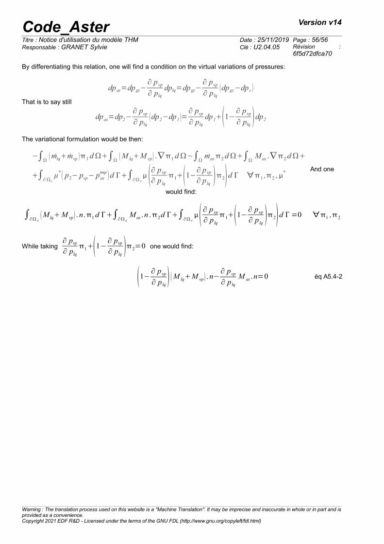
Code_Aster Version v14
Titre : Notice d'utilisation du modèle THM Date : 25/11/2019 Page : 56/56Responsable : GRANET Sylvie Clé : U2.04.05 Révision :
6f5d72dfca70
By differentiating this relation, one will find a condition on the virtual variations of pressures:
dpas=dpgz−∂ pvp
∂ plq
dplq=dpgz−∂ pvp
∂ p lqdpgz−dpc
That is to say still
dpas=dp2−∂ pvp
∂ plqdp2−dp1 =
∂ pvp
∂ plq
dp11−∂ pvp
∂ plqdp2
The variational formulation would be then:
−∫ mlqmvp 1d∫
M lqM vp .∇1d−∫mas2d∫
M as .∇2d
∫∂ d
μ* p2− pvp− pasimp d ∫
∂ d
∂ pvp
∂ p lq
11−∂ pvp
∂ p lq2d ∀1 ,2 ,
* And one
would find:
∫∂ d
M lqM vp .n.1d ∫∂ d
M as .n .2d ∫∂ d
∂ pvp
∂ p lq
11−∂ pvp
∂ p lq2d =0 ∀1 ,2
While taking ∂ pvp
∂ plq
11−∂ pvp
∂ plq2=0 one would find:
1−∂ pvp
∂ p lq M lqM vp .n−
∂ pvp
∂ p lq
M as .n=0 éq A5.4-2
Warning : The translation process used on this website is a "Machine Translation". It may be imprecise and inaccurate in whole or in part and isprovided as a convenience.Copyright 2021 EDF R&D - Licensed under the terms of the GNU FDL (http://www.gnu.org/copyleft/fdl.html)