Embed Size (px)
Citation preview
Note to Readers
This is an excerpt from Taming Indian Inflation.
High and persistent inflation has been a serious macroeconomic challenge for India, particularly in the past decade. India’s high rates of inflation have been underpinned chiefly by high and persistent rates of food price inflation, which cascade quickly into rural and urban wages and into nonfood inflation. This book takes a timely and in-depth look at the high and persistent inflation that has presented serious macroeconomic challenges to India in recent years—a situation that has helped to increase the country’s domestic and external vulnerabilities. The authors analyze various facets of Indian inflation and their implications for the Indian economy. Several chapters examine food inflation, given the very important role of food inflation in driving overall inflation dynamics in India. Building on this analysis of inflation dynamics, other chapters discuss the role of monetary policy in taming inflation. The book draws on the ongoing dialogue between the IMF staff and Indian authorities within the Reserve Bank of India and the Ministry of Finance. This excerpt is taken from uncorrected page proofs. Please check quotations and attributions against the published volume. Taming Indian Inflation Edited by Rahul Anand and Paul Cashin ISBN: 978-1-51354-125-9 Pub. Date: March 2016 Format: Digital; Paperback, 6 x 9 in., Approx. 240 pp. Price: US$30
For additional information on this book, please contact: International Monetary Fund, IMF Publications P.O. Box 92780, Washington, DC 20090, U.S.A.
Tel: (202) 623-7430 Fax: (202) 623-7201 Email: [email protected]
www.imfbookstore.org
© 2016 International Monetary Fund
© 2016 International Monetary Fund
Cover design: IMF Multimedia Services Division
Cataloging-in-Publication DataJoint Bank-Fund Library
Cashin, Paul. | Anand, Rahul. | International Monetary Fund.Taming inflation in India / editors: Paul Cashin, Rahul Anand.Washington, DC : International Monetary Fund, 2016. | Includes bibliographical references and index.
ISBN 978-1-51354-125-9 (paper) LCSH: Inflation (Finance) – India. | Food prices – India. | India – Economic conditions – 21st century.
LCC HG1232.5.T345 2016
The views expressed in this book are those of the authors and do not necessarily represent the views of the International Monetary Fund, its Executive Board, or IMF management.
Please send orders to:International Monetary Fund, Publication ServicesP.O. Box 92780, Washington, DC 20090, U.S.A.
Tel.: (202) 623-7430 Fax: (202) 623-7201E-mail: [email protected]: www.elibrary.imf.org
www.imfbookstore.org
iii
Table of Contents
Foreword v
Preface vii
PART I CAUSES OF INFLATION ....................................................................................1
1 Inflation Dynamics in India: What Can We Learn from Phillips Curves? ........3 Roberto F. Guimarães and Laura Papi
2 Reconsidering the Role of Food Prices in Inflation ......................................... 23 James P. Walsh
3 Food Inflation in India................................................................................................ 45 Prachi Mishra and Devesh Roy
4 Understanding India’s Food Inflation Through the Lens of Demand and Supply ..................................................................................................................... 75 Rahul Anand, Naresh Kumar, and Volodymyr Tulin
PART II CONSEQUENCES OF INFLATION .............................................................113
5 Does Inflation Slow Long-Run Growth in India? ............................................115 Kamiar Mohaddes and Mehdi Raissi
6 Inflation and Income Inequality: Is Food Inflation Different? ...................131 James P. Walsh and Jiangyan Yu
7 Transmission of India’s Inflation to Neighboring Countries ......................149 Sonali Das, Adil Mohommad, and Yasuhisa Ojima
PART III POLICIES TO AFFECT INFLATION ............................................................167
8 Monetary Policy Transmission in India ..............................................................169 Sonali Das
9 Food Inflation in India: What Role for Monetary Policy? .............................187 Rahul Anand and Volodymyr Tulin
10 Inflation and Monetary Policy in Small Open Economies ..........................201 Paul Cashin and Agustín Roitman
Contributors .............................................................................................................................223
Index ..........................................................................................................................................227

v
Foreword
This book is a timely look at an important Indian macroeconomic issue— inflation. High and persistent inflation has been a serious macroeconomic chal-lenge for India, particularly in the past decade. India’s high rates of inflation have been underpinned chiefly by high and persistent rates of food price inflation, which cascade quickly into rural and urban wages and into nonfood inflation. Well-entrenched inflation expectations have also been a key driver of India’s high inflation rates.
Over the past decade India has increasingly opened itself to the global econo-my and has become one of the world’s fastest-growing economies. As it seeks to sustain rapid growth and improve the welfare of its large and fast-growing popu-lation, India also needs to aim for greater price stability.
This book documents and analyzes India’s long-ongoing quest to bring infla-tion down. It grew out of the IMF staff ’s ongoing policy dialogue with the Indian authorities, in particular at the Reserve Bank of India and the Ministry of Finance. The focus of several of the chapters evolved from the exchange of views with officials from these agencies, and with the many Indian academics interested in these issues.
The IMF is contributing to the advancement of the Indian economy through our ongoing policy dialogue, analytical work, and capacity building. I am sure this book will help in this effort and give due recognition to the authorities’ efforts directed at taming inflation to reduce poverty, raise domestic consumption and growth, and improve the welfare of over 1.2 billion Indian citizens.
Christine LagardeManaging DirectorInternational Monetary Fund

vii
Preface
High and persistent inflation has presented a serious macroeconomic challenge in India in recent years, increasing the country’s domestic and external vulnerabili-ties. For example, high inflation contributed to an historic widening of the current account deficit, exposing India to global financial market turbulence and slowing growth. As Reserve Bank of India Governor Raghuram Rajan pointed out at the 8th R. N. Kao Memorial Lecture in 2014, “inflation is a destructive disease … we can’t push inflation under the carpet as a central banker. We have to deal with it.”
A number of factors underpin India’s high rates of inflation, including food inflation feeding quickly into wages and core inflation; entrenched inflation expectations; cost-push shocks from binding sector-specific supply constraints (particularly in agriculture, energy, and transportation); pass-through from a weaker rupee; and ongoing energy price increases. This book analyzes various facets of Indian inflation and their implications for the conduct of monetary policy. Indeed, several chapters are devoted to analyzing and managing food infla-tion, given the very important role of food inflation in driving overall inflation dynamics in India. Building on this analysis of inflation dynamics, several chap-ters discuss the role of monetary policy in taming inflation, which is important for the country given the economic and social costs of its high and persistent inflation.
Using the Phillips curve framework, Roberto Guimarães and Laura Papi, in Chapter 1, find that inflation in India can be reasonably well modeled with stan-dard Phillips curves, augmented with a measure of relative international com-modity prices. They show that India’s inflation dynamics are explained by both backward- and forward-looking inflation components, and that the output gap, though empirically relevant, is not robust across model specifications. Evidence suggests that the effect of the output gap on inflation is larger at higher levels of inflation, but that inflation becomes more inertial at higher levels.
Because food inflation has played a key role in shaping the dynamics of infla-tion in India, and made monetary management more difficult, the next few chapters delve deeper into analyzing food inflation. It is widely believed that fluctuations in food and energy prices represent supply shocks, and as such are transitory, volatile, and nonmonetary in nature. For these reasons, food prices are generally excluded from the measures of inflation most closely watched by policy-makers in advanced economies.
James Walsh, in Chapter 2, focuses on the role of food inflation in lower-income countries and emerging markets, and finds that food price inflation is not only more volatile in these economies, but also higher than nonfood inflation on average. Walsh shows that food inflation is in many cases more persistent than nonfood inflation, and that food price shocks in many countries propagate strongly into nonfood inflation. Under these conditions, a policy focus on
viii Preface
measures of core inflation that exclude food prices can misspecify inflation, lead-ing to higher inflationary expectations, a downward bias to forecasts of future inflation, and lags in policy responses. In constructing measures of core inflation, policymakers should therefore not assume that excluding food price inflation will provide a clearer picture of underlying inflation trends than headline inflation.
Chapter 3, by Prachi Mishra and Devesh Roy, examines food inflation in India using a high-frequency, commodity-level data set spanning the past two decades. Documenting stylized facts about the behavior of food inflation, the authors explicitly quantify the contribution of specific commodities to food inflation in India. Their analysis suggests that animal source foods (milk, fish), processed food (sugar, edible oils), fruits and vegetables (for example, onions), and cereals (rice and wheat) have been the primary drivers of food price inflation. Insights from this analysis of overall food inflation, as well as individual case studies, are used to make specific policy recommendations for curbing inflation.
In Chapter 4, Rahul Anand, Naresh Kumar, and Volodymyr Tulin investigate the demand and supply factors behind the contribution of relative food inflation to general inflation. They find that India’s food inflation developments over the past decade appear to have largely reflected demand pressures (driven by strong private consumption growth), which have often outpaced supply of key food commodities. Their analysis suggests that in the absence of a stronger food supply growth response, food inflation may exceed nonfood inflation by 2½–3 percent-age points per year. Given this, the sustainability of a long-term inflation target of 4 percent under India’s recently adopted flexible inflation-targeting framework will depend on enhancing food supply, agricultural market-based pricing, and reducing price distortions. A well-designed cereal buffer stock liquidation policy could also help mitigate food inflation volatility.
The next few chapters explore the costs of inflation in India—on both growth and inclusiveness—and document the spillovers of Indian inflation to the neigh-boring countries of Nepal and Bhutan. In Chapter 5, Kamiar Mohaddes and Mehdi Raissi examine the long-term relationship between the consumer price index for industrial workers (CPI-IW) inflation and GDP growth in India. Using a sample of 14 Indian states over 1989–2013, the chapter’s findings suggest that, on average, there is a negative long-term relationship between inflation and eco-nomic growth. The authors find there is a statistically significant inflation-growth threshold effect in states with persistently elevated consumer price index inflation rates of over 5½ percent. These findings suggest that the Reserve Bank of India needs to balance the short-term growth-inflation trade-off, in light of the long-term negative effects on growth of persistently high inflation.
In Chapter 6, James Walsh and Jiangyan Yu analyze the effects of inflation on income inequality, and find these can be differentiated by the type of inflation. Higher nonfood inflation is strongly associated with greater income inequality, but food inflation has more mixed effects. Across a sample of Indian states, non-food inflation is associated with worsening income inequality in both urban and rural areas. On the other hand, higher food inflation has an ambiguous
Preface ix
relationship with income inequality in urban areas, but is strongly associated with lower income inequality in rural areas.
Sonali Das, Adil Mohammad, and Yasuhisa Ojima, in Chapter 7, explore the spillovers of Indian inflation—particularly food inflation—on Nepal and Bhutan. Inflation dynamics in both countries are closely linked to those in India, given their exchange rate pegs to the Indian rupee. The authors suggest that food infla-tion in Nepal, a key driver of the country’s headline inflation, is highly correlated with food price changes in India. Similarly, headline inflation in Bhutan over the past three decades shows a tendency to comove with India’s headline CPI infla-tion rate. Given their exchange rate regimes and close trade ties with India, it is unlikely that inflation will be delinked from India in the near term.
Against a backdrop of the high cost of inflation and spillovers to neighboring countries, Chapters 8 and 9 discuss the role of monetary policy in taming India’s high and persistent inflation. Sonali Das, in Chapter 8, evaluates the effectiveness of the credit channel of monetary policy transmission. Using stepwise estimation of vector error correction models, she finds significant, albeit slow, pass-through of policy rate changes to bank interest rates, and evidence of asymmetric adjustment to monetary policy. Here, bank lending rates adjust more quickly to monetary tightening than to loosening. Moreover, the speed of adjustment of bank deposit and lending rates to changes in the policy rate has increased in recent years.
In Chapter 9, Rahul Anand and Volodymyr Tulin discuss the role of monetary policy in combating food inflation in India, as this has presented challenges for monetary management. It is a widely held view that central banks should only respond to changes in underlying core inflation and to any second-round effects on core inflation of commodity price shocks. This chapter estimates the size of these second-round effects and finds particularly large effects in India. The results also indicate that India’s inflation is highly inertial and persistent. The authors’ analysis suggests that to durably reduce India’s relatively high rates of inflation, the monetary policy stance needs to remain tight for a considerable length of time.
Paul Cashin and Agustín Roitman, in Chapter 10, examine the role of optimal monetary policy in the presence of large and persistent supply shocks. They show that responding to headline inflation is welfare superior to responding to core inflation, and that this often proves to be a more effective response in containing overall inflation, as well as in mitigating consumption and output fluctuations. Moreover, having a clear, easy-to-understand, and transparent rule can help with the formation of accurate and realistic inflation expectations, and serve as an effective nominal anchor in the face of international commodity price fluctua-tions. Implementing such a rule is also useful to build and enhance the credibil-ity of the monetary authority, and thereby increase the effectiveness of monetary policy in seeking to achieve and maintain price stability.

75
CHAPTER 4
Understanding India’s Food Inflation Through the Lens of Demand and Supply
Rahul anand, naResh KumaR, and VolodymyR Tulin
Food inflation in India, unlike in many advanced economies, has had a nontrivial impact on aggregate retail inflation. This reflects, among other things, the large share of food expenditure in total household expenditure and its correspondingly heavy weight in the consumer price index (CPI), inflation expectations which are anchored by food inflation, and wage indexation to consumer price inflation and thereby indirectly to food inflation.
The importance of these factors in shaping India’s inflation dynamics and determining the conduct of monetary policy, particularly of large second-round effects of food price shocks, has been documented (Anand, Ding, and Tulin 2014; RBI 2014a). However, there is no consensus on the possible drivers of persistently high food inflation in India. The relative importance of demand and supply fac-tors and the role of related nonmonetary policies—notably the role of minimum support prices and the Mahatma Gandhi National Rural Employment Guarantee Act—are still debated.
Gokarn (2011), in his comprehensive analysis of India’s key food price issues since the 1960s, concludes that when food prices rise while supply stagnates or fails to keep up, there is no alternative to curbing food inflation other than raising supply rapidly. Although many studies1 have investigated demand and supply of the major food commodities in India and projected demand and supply scenar-ios, even at the commodity level, analysis of food prices in an equilibrating demand-supply framework is practically nonexistent.
This chapter explores the relative role of demand and supply factors and quan-tifies their impact on the dynamics of food prices in India in a general equilibrium setting. To do this, we adopt a two-stage strategy. First, we estimate individual demand for major food product groups and examine key household consumption patterns using household expenditure surveys. We then construct a general equi-librium model for given output growth scenarios, allowing us to estimate the impact of demand-side pressure on relative food prices. Using this model, we estimate the size of relative food prices since 2006 and simulate possible scenarios
1 See Ganesh-Kumar and others (2012) for literature review, as well as for medium-term forecasts on India’s demand and supply gaps for food grains.
76 Understanding India’s Food Inflation Through the Lens of Demand and Supply
of the contribution of relative food inflation in the medium term. For scenario analysis, the approach of abstracting away from explicit modeling of food supply is not without limitations,2 and the estimated inflation outcomes are likely to have an upward bias. Nonetheless, as own-price supply elasticities (Kumar and others 2010) are found to be significantly below demand elasticities, effects on prices from shifts in demand are likely to be only minimally mitigated by response of supply, particularly over the near term.
Our results suggest that given the heavy weight of food in household expendi-ture, robust real income growth in the past decade has resulted in substantial demand-side pressures. Because the supply of key agricultural products did not keep pace with real personal consumption growth, growth in food prices has outpaced nonfood prices by about 3½ percent since 2006/07. And with real personal consumption growth expected to be robust and food supply relatively sluggish in the coming years, it seems that India’s inflation dynamics will continue to be shaped by the relative food price trend.
Our estimates suggest that in the absence of a stronger food supply growth response, relative food inflation can contribute about 1¼ percentage points to headline inflation annually. If private consumption picks up to 7 percent and supply growth response remains at its historical level, food inflation is likely to exceed nonfood inflation by 2½–3 percentage points per year. Monetary policy will therefore need to react appropriately to both supply shocks and underlying inflation trends, particularly in the context of the flexible inflation targeting adopted in February 2015. Achieving a long-term inflation target of 4 percent will hinge on enhancing food supply, market-based pricing of agricultural pro-duce, and reducing price distortions. Our simulation analysis also indicates that given India’s supply-side vulnerabilities, the recommended inflation band of ±2 percent appears broadly appropriate. A well-designed cereal buffer stock liquida-tion policy could help mitigate inflation volatility. In addition, administered price setting, such as through minimum support prices and supporting policies, will continue to pose challenges for monetary policy management in India. At the current juncture when relative food prices do not appear to be a key driver of headline inflation, ensuring a durable reduction in headline inflation will require the continuation of a relatively tight monetary stance to durably lower core inflation so as to sustainably reduce inflation expectations and anchor them at a lower level.
RECENT INFLATION DYNAMICS IN INDIAHigh and persistent inflation has been a key macroeconomic challenge facing India (IMF 2014a, 2014b; Anand, Ding, and Tulin 2014). Elevated inflation coinciding with the growth slowdown has distinguished India from other major emerging market economies in recent years. Though several reasons have been
2 As in an inelastic supply system, only price but not supply adjusts to equilibrate demand.
Anand, Kumar, and Tulin 77
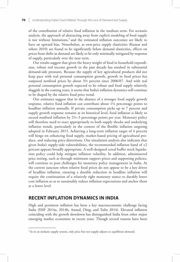
put forward to explain this persistently high inflation in India, food inflation has been often singled out as a key driver. Indeed, food inflation has exceeded non-food inflation by about 3½ percentage points on average during 2006/07–2013/14, contributing directly about 1¾ percentage points to headline CPI inflation (Figure 4.1). Furthermore, through its second-round effects on core inflation (Anand, Ding, and Tulin 2014), food inflation has added to the infla-tionary pressure.
INDIA’S FOOD INFLATION: A TIMELINEA chronological account of India’s food inflation reveals several important events, which have been widely documented and researched (Gokarn 2011; Sonna and others 2014):
• A set of policy interventions commonly known as the Green Revolution caused food inflation episodes to be short-lived and less intense during the 1980s and 1990s. These interventions combined price incentives, input subsidies, technological inputs and infrastructure investments (particularly in irrigation), and, importantly, buffer stocks. The policy interventions helped to raise and stabilize the productivity of cereal cultivation, as well as some other crops (Gokarn 2011).
Figure 4.1. Headline and Food Inflation(Year-over-year percent change)
20070
5
10
15
20
25
2008 2009 2010 2011 2012 2013 2014Sources: Haver Analytics; and IMF staff calculations.Note: CPI = consumer price index.
Food categories of CPI Headline CPI Nonfood CPI
78 Understanding India’s Food Inflation Through the Lens of Demand and Supply
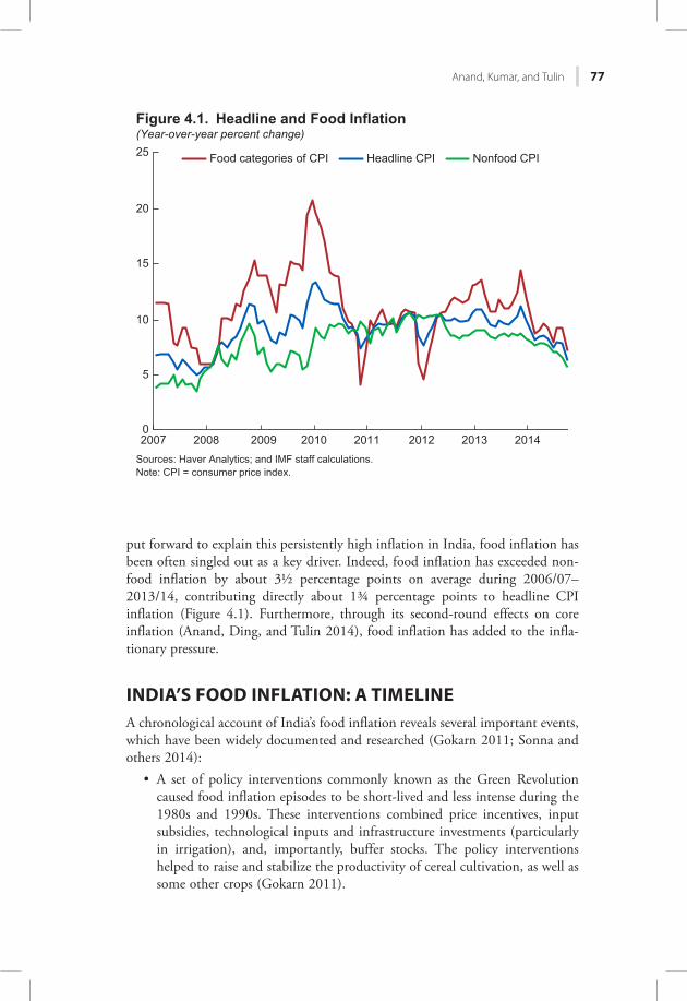
• However, during the 1990s and 2000s, agricultural growth slowed, averag-ing about 3.5 percent per year. Cereal yields grew by only 1½ percent per year in the 2000s. Amid firming consumer demand, running down buffer stocks helped contain food inflation during the early 2000s, as increases in minimum support prices moderated (Figure 4.2).
• The government’s response, beginning in 2007, to a surge in global food prices helped limit the impact on domestic food prices (OECD 2009). However, buffer stocks continued to fall, eventually to significantly below established norms. For example, around mid-2007, the wheat stock in the Central Pool amounted to only about half of the buffer stock norm. Moreover, a series of government measures—such as large increases in food and fertilizer subsidies, and an increase of more than 30 percent in minimum
1. Rice: buffer norms and actual stock in Central Pool(Million metric tonnes, as of January 1)
05
10152025303540
1992 1995 1998 2001 2004 2007 2010 2013
2. Wheat: buffer norms and actual stockin Central Pool(Million metric tonnes, as of January 1)
0510152025303540
1992 1995 1998 2001 2004 2007 2010 2013
3. Rice: minimum support and actual prices(Annual percent change, on crop-year basis)
Sources: Food Corporation of India; and IMF staff calculations.Note: In panels 3 and 4, crop year denotes a 12-month period from July through next June.MSP = minimum support price; WPI = wholesale price index.
–505
10152025303540
1992 1995 1998 2001 2004 2007 2010 2013
WPI, rice MSP
4. Wheat: minimum support and actual prices(Annual percent change, on crop-year basis)
–50510152025303540
1992 1995 1998 2001 2004 2007 2010 2013
Figure 4.2. Policy Interventions and Outcomes: Buffer Stocks of Rice and Wheat
Actual stock in Central Pool Buffer norm
Anand, Kumar, and Tulin 79
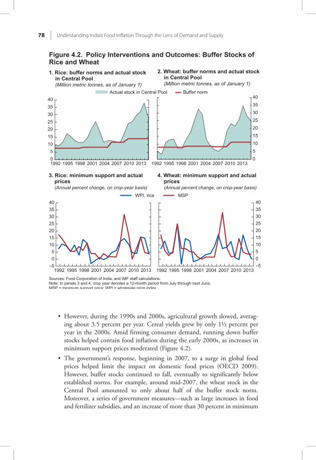
support prices for the 2008/09 season—likely not only postponed, but also prolonged inflationary pressures even after global food commodity prices abated (Figure 4.3). The global commodity price spike of 2007–08 also led to excessive stock hoarding in subsequent years, a shift in the buffer stock policy resulting in sustained inflationary pressure (Figure 4.2).3
• Deficient rainfall, as a result of weaker monsoon in 2009, affected the out-put of key agricultural crops and was an important factor behind elevated food inflation spilling into 2010 (RBI 2014b). Overall, growth in food inflation outpaced nonfood inflation by almost 30 percentage points during 2006–10: food inflation exceeded nonfood inflation on an average by almost 7½ percentage points per year during this period (Figure 4.3).
• Even though 2010 was a good monsoon year, food inflation remained high. Furthermore, despite 2011 being another relatively good monsoon year, food inflation surged again following a minor blip in food prices. This time, nonfood inflation also picked up, averaging 9½ percent during 2010–13, a full 3 percentage points higher than the average of 6½ percent during 2006–09.
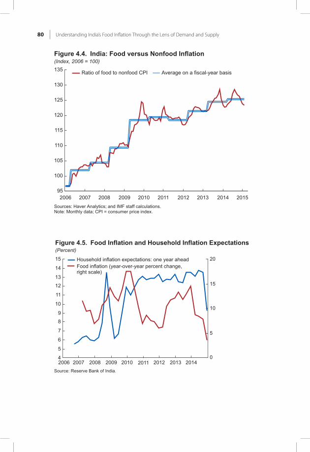
• Thus, even as relative food prices staged only a moderate gain during 2010–14, headline inflation remained high, driven by entrenched, elevated inflation expectations (Figure 4.4). This accelerated the inflationary spiral with food inflation feeding quickly into wages and core inflation (Figure 4.5).
3 In the aftermath of the surge in global commodity prices, not only food importers but also the larg-est exporters, namely China and India, became wary of overreliance on international grain markets, particularly in times of food emergency, which led to large-scale grain procurement and hoarding.
Source: IMF, International Financial Statistics database.
60
70
80
90
100
110
120
130
140
2006 2007 2008 2009 2010 2011 2012 2013 2014
Global food commodity price indexAverage on a fiscal-year basis
Figure 4.3. Global Food Commodity Prices(Index, 2010 = 100, U.S. dollar-based)
80 Understanding India’s Food Inflation Through the Lens of Demand and Supply
Figure 4.4. India: Food versus Nonfood Inflation(Index, 2006 = 100)
Sources: Haver Analytics; and IMF staff calculations.Note: Monthly data; CPI = consumer price index.
200695
100
105
110
115
120
125
130
135
2007 2008 2009 2010 2011 2012 2013 2014 2015
Ratio of food to nonfood CPI Average on a fiscal-year basis
Hkiwtg"6070 Hqqf"Kphncvkqp"cpf"Jqwugjqnf"Kphncvkqp"Gzrgevcvkqpu(Percent)
Source: Reserve Bank of India.
0
5
10
15
20
4
5
6
7
89
10
11
12
13
14
15
2006 2007 2008 2009 2010 2011 2012 2013 2014
Household inflation expectations: one year aheadFood inflation (year-over-year percent change,right scale)
Anand, Kumar, and Tulin 81
INDIA’S FOOD INFLATION: THE SUPPLY-DEMAND ANGLEWhile a number of supply-side factors could be responsible for food price pres-sures, they need to be scrutinized in the context of India’s growing food demand.
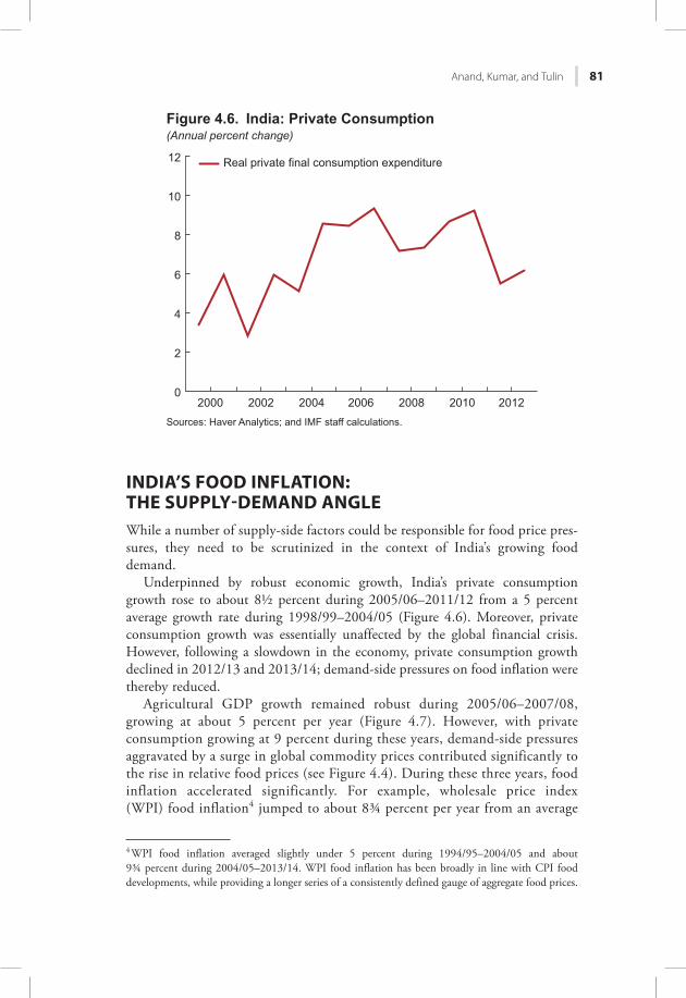
Underpinned by robust economic growth, India’s private consumption growth rose to about 8½ percent during 2005/06–2011/12 from a 5 percent average growth rate during 1998/99–2004/05 (Figure 4.6). Moreover, private consumption growth was essentially unaffected by the global financial crisis. However, following a slowdown in the economy, private consumption growth declined in 2012/13 and 2013/14; demand-side pressures on food inflation were thereby reduced.
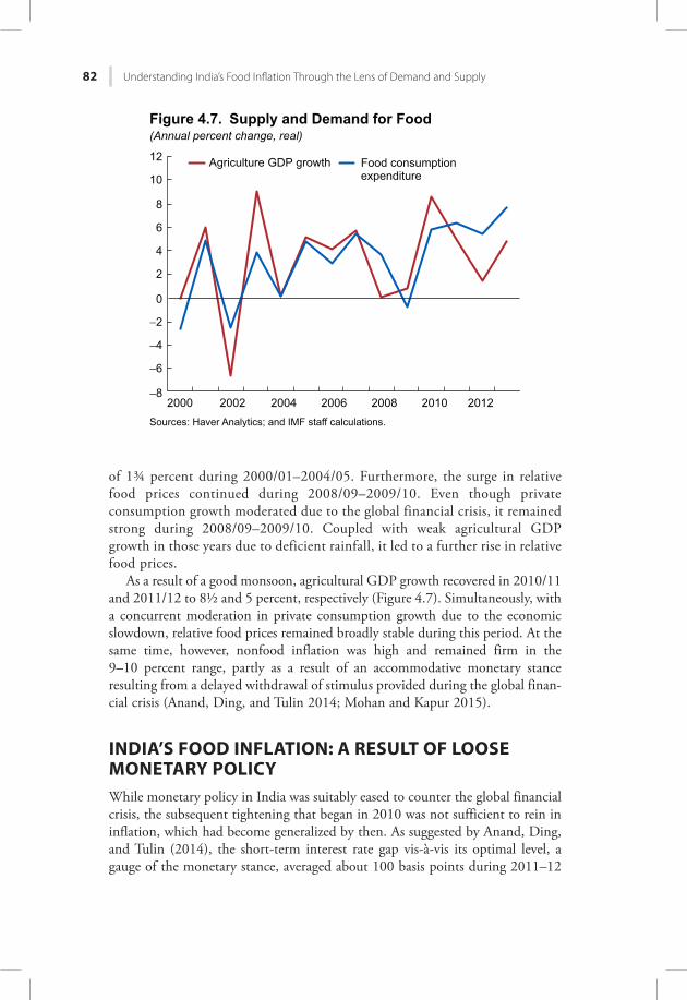
Agricultural GDP growth remained robust during 2005/06–2007/08, growing at about 5 percent per year (Figure 4.7). However, with private consumption growing at 9 percent during these years, demand-side pressures aggravated by a surge in global commodity prices contributed significantly to the rise in relative food prices (see Figure 4.4). During these three years, food inflation accelerated significantly. For example, wholesale price index (WPI) food inflation4 jumped to about 8¾ percent per year from an average
4 WPI food inflation averaged slightly under 5 percent during 1994/95–2004/05 and about 9¾ percent during 2004/05–2013/14. WPI food inflation has been broadly in line with CPI food developments, while providing a longer series of a consistently defined gauge of aggregate food prices.
Figure 4.6. India: Private Consumption(Annual percent change)
Sources: Haver Analytics; and IMF staff calculations.
0
2
4
6
8
10
12
2000 2002 2004 2006 2008 2010 2012
Real private final consumption expenditure
82 Understanding India’s Food Inflation Through the Lens of Demand and Supply
of 1¾ percent during 2000/01–2004/05. Furthermore, the surge in relative food prices continued during 2008/09–2009/10. Even though private consumption growth moderated due to the global financial crisis, it remained strong during 2008/09–2009/10. Coupled with weak agricultural GDP growth in those years due to deficient rainfall, it led to a further rise in relative food prices.
As a result of a good monsoon, agricultural GDP growth recovered in 2010/11 and 2011/12 to 8½ and 5 percent, respectively (Figure 4.7). Simultaneously, with a concurrent moderation in private consumption growth due to the economic slowdown, relative food prices remained broadly stable during this period. At the same time, however, nonfood inflation was high and remained firm in the 9–10 percent range, partly as a result of an accommodative monetary stance resulting from a delayed withdrawal of stimulus provided during the global finan-cial crisis (Anand, Ding, and Tulin 2014; Mohan and Kapur 2015).
INDIA’S FOOD INFLATION: A RESULT OF LOOSE MONETARY POLICYWhile monetary policy in India was suitably eased to counter the global financial crisis, the subsequent tightening that began in 2010 was not sufficient to rein in inflation, which had become generalized by then. As suggested by Anand, Ding, and Tulin (2014), the short-term interest rate gap vis-à-vis its optimal level, a gauge of the monetary stance, averaged about 100 basis points during 2011–12
Sources: Haver Analytics; and IMF staff calculations.
−8
−6
−4
−2
0
2
4
6
8
10
12
2000 2002 2004 2006 2008 2010 2012
Agriculture GDP growth Food consumptionexpenditure
Hkiwtg"6090 Uwrrn{"cpf"Fgocpf"hqt"Hqqf(Annual percent change, real)
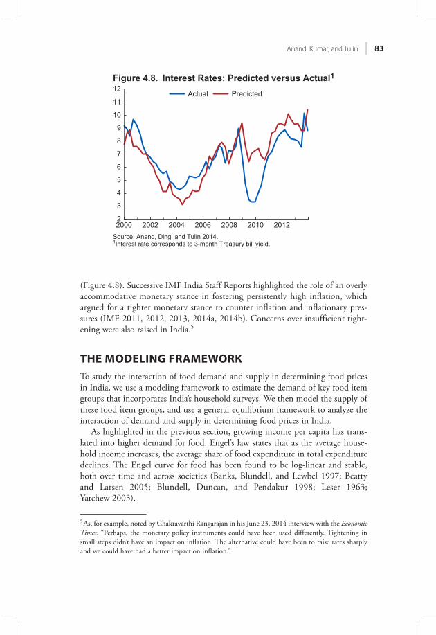
Anand, Kumar, and Tulin 83
(Figure 4.8). Successive IMF India Staff Reports highlighted the role of an overly accommodative monetary stance in fostering persistently high inflation, which argued for a tighter monetary stance to counter inflation and inflationary pres-sures (IMF 2011, 2012, 2013, 2014a, 2014b). Concerns over insufficient tight-ening were also raised in India.5
THE MODELING FRAMEWORKTo study the interaction of food demand and supply in determining food prices in India, we use a modeling framework to estimate the demand of key food item groups that incorporates India’s household surveys. We then model the supply of these food item groups, and use a general equilibrium framework to analyze the interaction of demand and supply in determining food prices in India.
As highlighted in the previous section, growing income per capita has trans-lated into higher demand for food. Engel’s law states that as the average house-hold income increases, the average share of food expenditure in total expenditure declines. The Engel curve for food has been found to be log-linear and stable, both over time and across societies (Banks, Blundell, and Lewbel 1997; Beatty and Larsen 2005; Blundell, Duncan, and Pendakur 1998; Leser 1963; Yatchew 2003).
5 As, for example, noted by Chakravarthi Rangarajan in his June 23, 2014 interview with the Economic Times: “Perhaps, the monetary policy instruments could have been used differently. Tightening in small steps didn’t have an impact on inflation. The alternative could have been to raise rates sharply and we could have had a better impact on inflation.”
Source: Anand, Ding, and Tulin 2014.1Interest rate corresponds to 3-month Treasury bill yield.
2
3
4
5
6
7
8
9
10
11
12
2000 2002 2004 2006 2008 2010 2012
Actual Predicted
Figure 4.8. Interest Rates: Predicted versus Actual1
84 Understanding India’s Food Inflation Through the Lens of Demand and Supply
Household Demand Analysis
Our food demand modeling approach relies on a two-stage budgeting frame-work, which assumes that consumers allocate their income in two steps. In the first, they decide on spending across broad categories of goods or services—our model entails a choice between food and nonfood. Each consumer decides on how much to spend on food items and nonfood items. In the second step, each consumer simultaneously decides on how to allocate the total food expenditure across specific food categories; for example, how much of the food expenditure budget will be spent on pulses versus how much on milk prod-ucts. We look at six food item groups: cereals; pulses; milk; egg, fish and meat; vegetables and fruits; and a category that includes oil and fats, sugar, condi-ments, and spices.
The two-stage approach invokes the block independence idea or strong group-separability assumption of the consumer preference theory, which implies that preferences among items within one broad consumption group are not dependent on the quantities consumed within other broad consumption groups. In other words, demand for specific nonfood items is not influenced by demand decisions for specific food items. A simple first-stage budgeting, which involves a choice between only two broad expenditure groups (namely, food and nonfood), allows us to greatly simplify the econometric estimation. The added condition of the expenditure weights—that the budget share on food and nonfood adds up to unity—implies that the first-stage estimation can be reduced to a single equation least squares regression with coefficient restrictions rather than the estimation of a system of equations.
However, when it comes to spending decisions within specific expenditure categories, understanding demand for several food items requires demand model-ing using a system of equations approach. This is important given that indepen-dent demand equations for various food items will not capture appropriately the demand for individual food items, as different food products can be substitutes or complements with important cross-price effects. A system of equations approach is, therefore, employed to estimate the demand of various food items within the broader food category. Overall, the two-stage budgeting procedure allows us to use reasonable assumptions regarding consumer behavior—the separability of con-sumer choice with respect to aggregate food and nonfood consumption and the consumption of various food items, while preserving some important characteris-tics of demand for various food items.
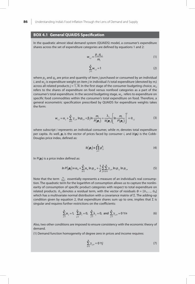
More specifically, to investigate the consumption patterns of Indian house-holds, we employ a two-stage quadratic almost ideal demand system (QUAIDS) model (Banks, Blundell, and Lewbel 1997). QUAIDS is an extension of the almost ideal demand system (AIDS) approach (Deaton and Muellbauer 1980) that includes a quadratic expenditure term to model nonlinearity of Engel curves. In the literature, AIDS-based approaches have been the preferred specification for estimating demand systems, owing to their consistency with consumer theory, exact aggregation properties, and ease of estimation. QUAIDS extensions, which
Anand, Kumar, and Tulin 85
provide a more accurate picture of consumer behavior across income groups, have proven useful in studying consumer food demand patterns, including those in India (Mittal 2010).
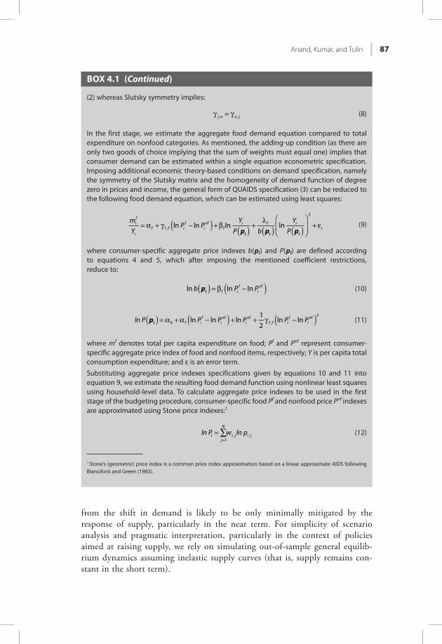
The first stage of QUAIDS involves estimating a first-step budgeting equation, whereby consumers make a choice about how much total expenditure will be devoted to food, conditional on the consumption of nonfood goods and services, and the demographic and socioeconomic characteristics of households. The non-linearity in food expenditure—implying that a relatively lower share of income will be spent on food as income increases—is modeled through a quadratic expenditure term. Because we focus on only two broad categories of consumer expenditure—food and nonfood—the adding-up restriction on the expenditure weights implies that the first-stage estimation is reduced to a single equation least squares estimation. See Annex 4.1 for additional details.
In the second stage, we estimate a system of simultaneous equations, each representing demand for specific food item categories (cereals; pulses; milk; egg, fish, and meat; vegetables and fruits; and others). Here, we specify a QUAIDS system of individual food item demand equations (see for example, Poi 2002, 2008) using the general QUAIDS structure outlined in Box 4.1, where expenditure weights represent expenditure on specific food categories as a share of the consumer’s total expenditure on food. In turn, the value of a consumer’s total expenditure on food is the predicted value of aggregate food expenditure from the first-stage estimation results. Given consumer choice over multiple food items, the second-stage QUAIDS specification is estimated as a system of nonlinear, seemingly unrelated regressions through iterated feasible generalized least squares, using the Stata routine described in Poi (2008).
Supply Analysis
The consumer demand model we use for estimation and simulation purposes assumes that prices, food prices in particular, are predetermined. The exogeneity of prices, which we assume, is rather common in demand system modeling. From the aggregate economy perspective, this is equivalent to assuming that supply is perfectly elastic in prices, and that it is demand that adjusts to clear the markets.6 A perfectly elastic supply and market-clearing demand is an appropri-ate assumption when dealing with traded goods, such as imported foods, in the case of small open economies. Of course, such assumptions may be somewhat unrealistic for the analysis of food supply in a country like India.
Nonetheless, studies of the supply of food commodities production in India suggest that own-price elasticities are low, particularly compared to own-price elasticities of demand (Kumar and others 2010). Therefore, the effect on prices
6 Inelastic supply assumptions are usually more suitable to analyze demand for goods with fixed prices, as a result of administered price setting.
86 Understanding India’s Food Inflation Through the Lens of Demand and Supply
BOX 4.1 General QUAIDS Specification
In the quadratic almost ideal demand system (QUAIDS) model, a consumer’s expenditure shares across the set of expenditure categories are defined by equations 1 and 2:
wp q
mi ji j i j
i,
, ,= (1)
w 1j
N
i j1
,∑ ==
(2)
where pi,j and qi,j are price and quantity of item j purchased or consumed by an individual i, and wi,j is expenditure weight on item j in individual i’s total expenditure (denoted by mi)across all related products j = 1, N. In the first stage of the consumer budgeting choice, wi,j refers to the shares of expenditure on food versus nonfood categories as a part of the consumer’s total expenditure. In the second budgeting stage, wi,j refers to expenditure on specific food commodities within the consumer’s total expenditure on food. Therefore, a general econometric specification prescribed by QUAIDS for expenditure weights takes the form:
p p p
w p lnm
P bm
Pln ln
i i ii j j
n
N
j n i n ji j i
i j,1
, ,
2
,∑ ( ) ( ) ( )= α + γ + β +λ
+ ϑ=
(3)
where subscript i represents an individual consumer, while mi denotes total expenditure per capita. As well, pi is the vector of prices faced by consumer i, and b(pi) is the Cobb-Douglas price index, defined as:
pb pi
j
N
i j1
,j∏( ) ≡
=
β (4)
In P(pi) is a price index defined as:
pln P p p pln
12
ln lnin
N
i nj
N
n
N
j n i j i n01
n ,1 1
, , ,∑ ∑∑( ) ≡ α + α + γ= = =
(5)
Note that the term miP pi( ) essentially represents a measure of an individual’s real consump-
tion. The quadratic term for the logarithm of consumption allows us to capture the nonlin-earity of consumption of specific product categories with respect to total expenditure on related products. Ji,j denotes a residual term, with the vector of residuals J = [J1,…, JN] which has a multivariate normal distribution with a covariance matrix of Σ. The adding-up condition given by equation 2, that expenditure shares sum up to one, implies that Σ is singular and requires further restrictions on the coefficients:
n1, 0, 0, and 0
j
N
jj
N
jj
N
jj
N
j n1 1 1 1
,∑ ∑ ∑ ∑α = β = λ = γ = ∀= = = =
(6)
Also, two other conditions are imposed to ensure consistency with the economic theory of demand.(1) Demand function homogeneity of degree zero in prices and income requires:
j0
n
N
j n1
,∑γ = ∀=
(7)
Anand, Kumar, and Tulin 87
BOX 4.1 (Continued)
(2) whereas Slutsky symmetry implies:
j n n j, ,γ = γ (8)
In the first stage, we estimate the aggregate food demand equation compared to total expenditure on nonfood categories. As mentioned, the adding-up condition (as there are only two goods of choice implying that the sum of weights must equal one) implies that consumer demand can be estimated within a single equation econometric specification. Imposing additional economic theory-based conditions on demand specification, namely the symmetry of the Slutsky matrix and the homogeneity of demand function of degree zero in prices and income, the general form of QUAIDS specification (3) can be reduced to the following food demand equation, which can be estimated using least squares:
p p p
mY
P PY
P bY
Pln ln ln ln
i i i
if
if f f i
finf
fi f i
i,
2
( ) ( ) ( ) ( )= α + γ − + β +λ
+ ε (9)
where consumer-specific aggregate price indexes b(pi) and P(pi) are defined according to equations 4 and 5, which after imposing the mentioned coefficient restrictions, reduce to:
pb P Pln ln lni f i
finf( )( ) = β − (10)
pln P P P P P Pln ln ln
12
ln lni f if
inf
inf
f f if
inf
0 ,
2( ) ( )( ) = α + α − + + γ − (11)
where mf denotes total per capita expenditure on food; Pf and Pnf represent consumer-specific aggregate price index of food and nonfood items, respectively; Y is per capita total consumption expenditure; and ε is an error term.Substituting aggregate price indexes specifications given by equations 10 and 11 into equation 9, we estimate the resulting food demand function using nonlinear least squares using household-level data. To calculate aggregate price indexes to be used in the first stage of the budgeting procedure, consumer-specific food Pf and nonfood price Pnf indexes are approximated using Stone price indexes:1
ln P w ln pi
j
N
i j i j1
, ,∑==
(12)
1 Stone’s (geometric) price index is a common price index approximation based on a linear approximate AIDS following Blanciforti and Green (1983).
from the shift in demand is likely to be only minimally mitigated by the response of supply, particularly in the near term. For simplicity of scenario analysis and pragmatic interpretation, particularly in the context of policies aimed at raising supply, we rely on simulating out-of-sample general equilib-rium dynamics assuming inelastic supply curves (that is, supply remains con-stant in the short term).
88 Understanding India’s Food Inflation Through the Lens of Demand and Supply
RESULTS AND DISCUSSIONHousehold Demand for Food
Results of the regression analysis are reported in Annex 4.1, and Box 4.2 explains how to interpret these coefficients.
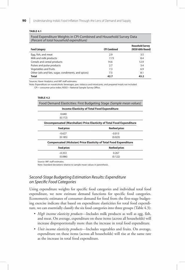
We focus on six food categories representing key food groups in the Indian household consumption basket: milk and milk products; egg, fish, and meat; pulses; cereals; vegetables and fruits; and a category of other foods that includes oil and fats, sugar, condiments, and spices. The choice of these categories is driven by distinct government policies, such as those related to production, pricing, and provision, toward these sectors. These food categories together correspond to about 43 percent of household consumption expenditure, both in the CPI and in the household survey data.7 Estimated expenditure weights on key food categories in the latest household survey (National Sample Survey Office 68th round for 2011/12) closely track weights in CPI Combined (Table 4.1), supporting the suitability of household-survey-based analysis to study implications of food demand dynamics for CPI inflation in India.
First-Stage Budgeting Estimation Results: Total Expenditure on Food
Estimates of consumer demand for food from the first-stage budgeting exercise indicate clear heterogeneity in food demand patterns across the income spectrum of Indian households.
The estimates suggest that as income per capita goes up by 1 percent, the demand for food rises by 0.64 percent (Table 4.2). Similarly, a 1 percent increase in food prices results in a 0.62 percent decline in total food expenditure when the consumer is not compensated for the price increase. However, if the consumer is compensated to maintain the same level of welfare, the total expenditure on food goes down by 0.35 percent when food prices rise by 1 percent.
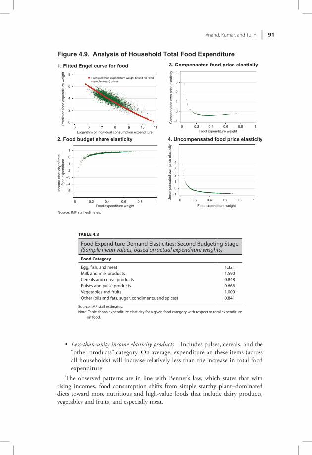
Panel 1 of Figure 4.9 plots the weights of food expenditure (predicted by our model) against the log of individual incomes. As predicted by Engel’s law, as income increases, households spend less and less on food (estimated weights on food expenditure declines). Panel 2 suggests that households spending a lot on food (high weight on food expenditure) also have high income elasticity of food expenditure. Panels 1 and 2 together suggest that the demand for food by poorer households goes up by more than for richer households when income per capita rises. Panels 3 and 4 of Figure 4.9 present price elasticities of food for food expen-diture weights. The results suggest that the elasticity is relatively large for those who spend a lot on food.
7 Note that CPI expenditure categories, commonly attributed to the food basket, such as beverages (2 percent CPI weight), prepared meals (2.8 percent), and pan, tobacco, and intoxicants (2.1 percent), are excluded from the analysis.
Anand, Kumar, and Tulin 89
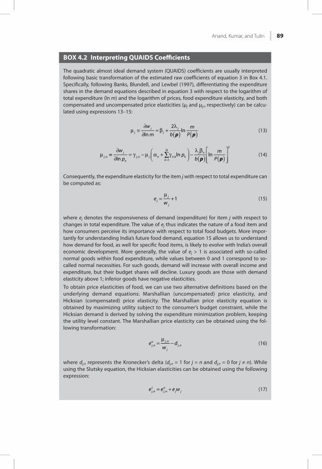
BOX 4.2 Interpreting QUAIDS Coefficients
The quadratic almost ideal demand system (QUAIDS) coefficients are usually interpreted following basic transformation of the estimated raw coefficients of equation 3 in Box 4.1. Specifically, following Banks, Blundell, and Lewbel (1997), differentiating the expenditure shares in the demand equations described in equation 3 with respect to the logarithm of total expenditure (ln m) and the logarithm of prices, food expenditure elasticity, and both compensated and uncompensated price elasticities (μj and μj,n respectively) can be calcu-lated using expressions 13–15:
p p
w
m bm
Pln
2lnj
jj
j
( ) ( )µ ≡∂
∂= β +
λ (13)
p p
w
pp
bm
Plnln lnj n
j
nj n j n
k
N
n kj n
, ,1
,k
2
∑ ( ) ( )µ ≡∂
∂= γ − µ α + γ
−λ β
=
(14)
Consequently, the expenditure elasticity for the item j with respect to total expenditure can be computed as:
e
w1j
j
j
=µ
+ (15)
where ej denotes the responsiveness of demand (expenditure) for item j with respect to changes in total expenditure. The value of ej thus indicates the nature of a food item and how consumers perceive its importance with respect to total food budgets. More impor-tantly for understanding India’s future food demand, equation 15 allows us to understand how demand for food, as well for specific food items, is likely to evolve with India’s overall economic development. More generally, the value of ej > 1 is associated with so-called normal goods within food expenditure, while values between 0 and 1 correspond to so-called normal necessities. For such goods, demand will increase with overall income and expenditure, but their budget shares will decline. Luxury goods are those with demand elasticity above 1; inferior goods have negative elasticities.To obtain price elasticities of food, we can use two alternative definitions based on the underlying demand equations: Marshallian (uncompensated) price elasticity, and Hicksian (compensated) price elasticity. The Marshallian price elasticity equation is obtained by maximizing utility subject to the consumer’s budget constraint, while the Hicksian demand is derived by solving the expenditure minimization problem, keeping the utility level constant. The Marshallian price elasticity can be obtained using the fol-lowing transformation:
e
wdj n
j n
jj n,
u ,,=
µ− (16)
where dj,n represents the Kronecker’s delta (dj,n = 1 for j = n and dj,n = 0 for j ≠ n). While using the Slutsky equation, the Hicksian elasticities can be obtained using the following expression:
e e e wj n j n j j,
c,
u= + (17)
90 Understanding India’s Food Inflation Through the Lens of Demand and Supply
Second-Stage Budgeting Estimation Results: Expenditure on Specific Food Categories
Using expenditure weights for specific food categories and individual total food expenditure, we now estimate demand functions for specific food categories. Econometric estimates of consumer demand for food from the first-stage budget-ing exercise indicate that based on expenditure elasticities for total food expendi-ture, we can essentially classify the six food categories into three groups (Table 4.3):
• High income elasticity products—Includes milk products as well as egg, fish, and meat. On average, expenditure on these items (across all households) will increase disproportionally more than the increase in total food expenditure.
• Unit income elasticity products—Includes vegetables and fruits. On average, expenditure on these items (across all households) will rise at the same rate as the increase in total food expenditure.
TABLE 4.1
Food Expenditure Weights in CPI-Combined and Household Survey Data (Percent of total household expenditure)
Food Category CPI CombinedHousehold Survey (NSSO 68th Round)
Egg, fish, and meat 2.9 3.5Milk and milk products 7.73 8.4Cereals and cereal products 14.6 12.9Pulses and pulse products 2.7 3.4Vegetables and fruits 7.3 6.9Other (oils and fats, sugar, condiments, and spices) 7.5 8.1Total 42.7 43.2
Sources: Haver Analytics; and IMF staff estimates.Note: Expenditure on nonalcoholic beverages, pan, tobacco and intoxicants, and prepared meals not included.
CPI = consumer price index; NSSO = National Sample Survey Office.
TABLE 4.2
Food Demand Elasticities: First Budgeting Stage (Sample mean values)
Income Elasticity of Total Food Expenditure
0.640(0.172)
Uncompensated (Marshalian) Price Elasticity of Total Food Expenditure
Food prices Nonfood prices
–0.627 –0.013(0.185) (0.023)
Compensated (Hicksian) Price Elasticity of Total Food Expenditure
Food prices Nonfood prices
–0.353 0.267(0.086) (0.122)
Source: IMF staff estimates.Note: Standard deviations relative to sample mean values in parenthesis.
Anand, Kumar, and Tulin 91
50
2
4
6
8
1. Fitted Engel curve for food
Figure 4.9. Analysis of Household Total Food Expenditure
6 7 8Logarithm of individual consumption expenditure
Pre
dict
ed fo
od e
xpen
ditu
re w
eigh
t
0 0.2 0.4 0.6 0.8 1
–5
–4
–3
–2
–1
0
1
2. Food budget share elasticity
Food expenditure weight
Inco
me
elas
ticity
of t
otal
fo
od e
xpen
ditu
re
Source: IMF staff estimates.
3. Compensated food price elasticity
0 0.2 0.4 0.6 0.8 1Food expenditure weight
–1
0
1
2
3
4
Com
pens
ated
ow
n pr
ice
elas
ticity
4. Uncompensated food price elasticity
Food expenditure weight0 0.2 0.4 0.6 0.8 1
–1
0
1
2
3
4
Unc
ompe
nsat
ed o
wn
pric
e el
astic
ity
9 10 11
Predicted food expenditure weight based on fixed(sample mean) prices
TABLE 4.3
Food Expenditure Demand Elasticities: Second Budgeting Stage (Sample mean values, based on actual expenditure weights)Food Category
Egg, fish, and meat 1.321Milk and milk products 1.590Cereals and cereal products 0.848Pulses and pulse products 0.666Vegetables and fruits 1.000Other (oils and fats, sugar, condiments, and spices) 0.841
Source: IMF staff estimates.Note: Table shows expenditure elasticity for a given food category with respect to total expenditure
on food.
• Less-than-unity income elasticity products—Includes pulses, cereals, and the “other products” category. On average, expenditure on these items (across all households) will increase relatively less than the increase in total food expenditure.
The observed patterns are in line with Bennet’s law, which states that with rising incomes, food consumption shifts from simple starchy plant–dominated diets toward more nutritious and high-value foods that include dairy products, vegetables and fruits, and especially meat.
92 Understanding India’s Food Inflation Through the Lens of Demand and Supply
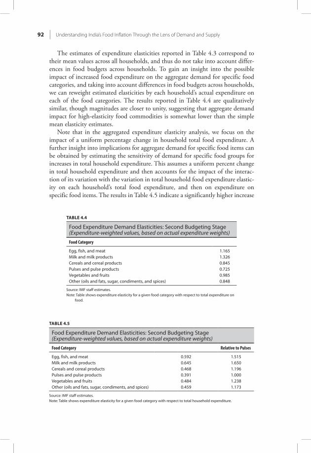
The estimates of expenditure elasticities reported in Table 4.3 correspond to their mean values across all households, and thus do not take into account differ-ences in food budgets across households. To gain an insight into the possible impact of increased food expenditure on the aggregate demand for specific food categories, and taking into account differences in food budgets across households, we can reweight estimated elasticities by each household’s actual expenditure on each of the food categories. The results reported in Table 4.4 are qualitatively similar, though magnitudes are closer to unity, suggesting that aggregate demand impact for high-elasticity food commodities is somewhat lower than the simple mean elasticity estimates.
Note that in the aggregated expenditure elasticity analysis, we focus on the impact of a uniform percentage change in household total food expenditure. A further insight into implications for aggregate demand for specific food items can be obtained by estimating the sensitivity of demand for specific food groups for increases in total household expenditure. This assumes a uniform percent change in total household expenditure and then accounts for the impact of the interac-tion of its variation with the variation in total household food expenditure elastic-ity on each household’s total food expenditure, and then on expenditure on specific food items. The results in Table 4.5 indicate a significantly higher increase
TABLE 4.4
Food Expenditure Demand Elasticities: Second Budgeting Stage (Expenditure-weighted values, based on actual expenditure weights)
Food Category
Egg, fish, and meat 1.165Milk and milk products 1.326Cereals and cereal products 0.845Pulses and pulse products 0.725Vegetables and fruits 0.985Other (oils and fats, sugar, condiments, and spices) 0.848
Source: IMF staff estimates.Note: Table shows expenditure elasticity for a given food category with respect to total expenditure on
food.
TABLE 4.5
Food Expenditure Demand Elasticities: Second Budgeting Stage (Expenditure-weighted values, based on actual expenditure weights)
Food Category Relative to Pulses
Egg, fish, and meat 0.592 1.515Milk and milk products 0.645 1.650Cereals and cereal products 0.468 1.196Pulses and pulse products 0.391 1.000Vegetables and fruits 0.484 1.238Other (oils and fats, sugar, condiments, and spices) 0.459 1.173
Source: IMF staff estimates.Note: Table shows expenditure elasticity for a given food category with respect to total household expenditure.
Anand, Kumar, and Tulin 93
in demand for milk and milk products and the category of egg, fish, and meat compared to pulses (the lowest-elasticity product category), with relative elastici-ties of 1.7 and 1.5, respectively. Moreover, each of the corresponding budget elasticities for cereals, vegetables and fruits, as well as other food categories is about 1.2 times higher than the budget elasticity of pulses, suggesting that the relative demand pressures for some food categories can be significantly higher as household incomes grow.
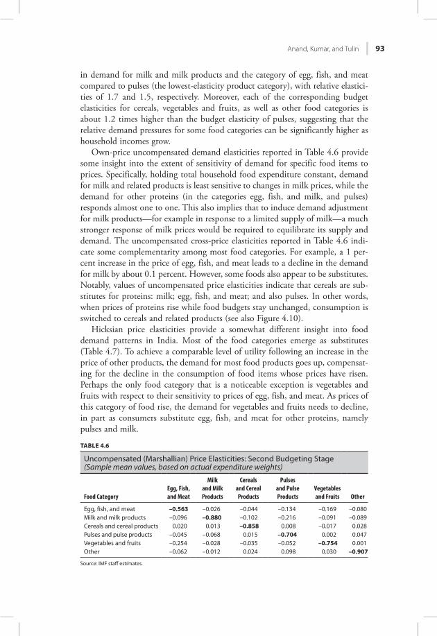
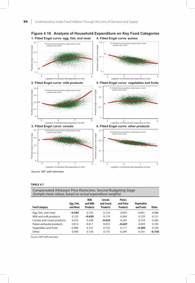
Own-price uncompensated demand elasticities reported in Table 4.6 provide some insight into the extent of sensitivity of demand for specific food items to prices. Specifically, holding total household food expenditure constant, demand for milk and related products is least sensitive to changes in milk prices, while the demand for other proteins (in the categories egg, fish, and milk, and pulses) responds almost one to one. This also implies that to induce demand adjustment for milk products—for example in response to a limited supply of milk—a much stronger response of milk prices would be required to equilibrate its supply and demand. The uncompensated cross-price elasticities reported in Table 4.6 indi-cate some complementarity among most food categories. For example, a 1 per-cent increase in the price of egg, fish, and meat leads to a decline in the demand for milk by about 0.1 percent. However, some foods also appear to be substitutes. Notably, values of uncompensated price elasticities indicate that cereals are sub-stitutes for proteins: milk; egg, fish, and meat; and also pulses. In other words, when prices of proteins rise while food budgets stay unchanged, consumption is switched to cereals and related products (see also Figure 4.10).
Hicksian price elasticities provide a somewhat different insight into food demand patterns in India. Most of the food categories emerge as substitutes (Table 4.7). To achieve a comparable level of utility following an increase in the price of other products, the demand for most food products goes up, compensat-ing for the decline in the consumption of food items whose prices have risen. Perhaps the only food category that is a noticeable exception is vegetables and fruits with respect to their sensitivity to prices of egg, fish, and meat. As prices of this category of food rise, the demand for vegetables and fruits needs to decline, in part as consumers substitute egg, fish, and meat for other proteins, namely pulses and milk.
TABLE 4.6
Uncompensated (Marshallian) Price Elasticities: Second Budgeting Stage (Sample mean values, based on actual expenditure weights)
Food CategoryEgg, Fish, and Meat
Milk and Milk Products
Cereals and Cereal Products
Pulses and Pulse Products
Vegetables and Fruits Other
Egg, fish, and meat –0.563 –0.026 –0.044 –0.134 –0.169 –0.080Milk and milk products –0.096 –0.880 –0.102 –0.216 –0.091 –0.089Cereals and cereal products 0.020 0.013 –0.858 0.008 –0.017 0.028Pulses and pulse products –0.045 –0.068 0.015 –0.704 0.002 0.047Vegetables and fruits –0.254 –0.028 –0.035 –0.052 –0.754 0.001Other –0.062 –0.012 0.024 0.098 0.030 –0.907
Source: IMF staff estimates.
94 Understanding India’s Food Inflation Through the Lens of Demand and Supply
5
0
0.1
Pre
dict
ed w
eigh
t in
food
bud
get
0.2
0.3
1. Fitted Engel curve: egg, fish, and meat
2. Fitted Engel curve: milk products
3. Fitted Engel curve: cereals
Figure 4.10. Analysis of Household Expenditure on Key Food Categories
0
0.1
Pre
dict
ed w
eigh
t in
food
bud
get
0.2
0.3
0.4
0
0.1
Pre
dict
ed w
eigh
t in
food
bud
get
0.2
0.3
0.4
6Logarithm of individual total expenditure on food
7 8
5 6Logarithm of individual total expenditure on food
7 8
5 6
Logarithm of individual total expenditure on food
7 8
Predicted food expenditure weight based on fixed(sample mean) prices
Predicted food expenditure weight based on fixed(sample mean) prices
Predicted food expenditure weight based on fixed(sample mean) prices
Source: IMF staff estimates.
Source: IMF staff estimates.
5. Fitted Engel curve: vegetables and fruits
6. Fitted Engel curve: other products
4. Fitted Engel curve: pulses
0
0.1
Pre
dict
ed w
eigh
t in
food
bud
get
0.2
5 6Logarithm of individual total expenditure on food
7 8
Predicted food expenditure weight based on fixed(sample mean) prices
0
0.1
Pre
dict
ed w
eigh
t in
food
bud
get
0.2
0.3
5 6Logarithm of individual total expenditure on food
7 8
Predicted food expenditure weight based on fixed(sample mean) prices
0
0.1
Pre
dict
ed w
eigh
t in
food
bud
get
0.2
0.3
5 6Logarithm of individual total expenditure on food
7 8
Predicted food expenditure weight based on fixed(sample mean) prices
TABLE 4.7
Compensated (Hicksian) Price Elasticities: Second Budgeting Stage (Sample mean values, based on actual expenditure weights)
Food CategoryEgg, Fish, and Meat
Milk and Milk Products
Cereals and Cereal Products
Pulses and Pulse Products
Vegetables and Fruits Other
Egg, fish, and meat –0.395 0.142 0.124 0.034 –0.001 0.088Milk and milk products 0.125 –0.659 0.119 0.004 0.129 0.131Cereals and cereal products 0.255 0.248 –0.623 0.243 0.218 0.263Pulses and pulse products 0.012 –0.011 0.072 –0.647 0.059 0.105Vegetables and fruits –0.086 0.141 0.133 0.117 –0.585 0.169Other 0.090 0.139 0.175 0.249 0.181 –0.756
Source: IMF staff estimates.
Anand, Kumar, and Tulin 95
Food Subsidies and Some Distributional Aspects
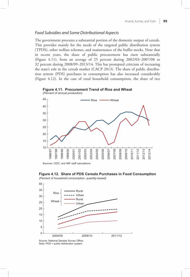
The government procures a substantial portion of the domestic output of cereals. This provides mainly for the needs of the targeted public distribution system (TPDS), other welfare schemes, and maintenance of the buffer stocks. Note that in recent years, the share of public procurement has risen substantially (Figure 4.11), from an average of 25 percent during 2002/03–2007/08 to 32 percent during 2008/09–2013/14. This has prompted criticism of increasing the state’s role in the cereals market (CACP 2013). The share of public distribu-tion system (PDS) purchases in consumption has also increased considerably (Figure 4.12). In the case of rural household consumption, the share of rice
10
15
20
25
30
35
40
45
1996
/97
1997
/98
1998
/99
1999
/00
2000
/01
2001
/02
2002
/03
2003
/04
2004
/05
2005
/06
2006
/07
2007
/08
2008
/09
2009
/10
2010
/11
2011
/12
2012
/13
2013
/14
Rice Wheat
Sources: CEIC; and IMF staff calculations.
Figure 4.11. Procurement Trend of Rice and Wheat(Percent of annual production)
0
5
10
15
20
25
30
35
40
2004/05 2009/10 2011/12
RuralUrbanRuralUrban
Rice
Wheat
Figure 4.12. Share of PDS Cereals Purchases in Food Consumption(Percent of household consumption, quantity-based)
Source: National Sample Survey Office.Note: PDS = public distribution system.
96 Understanding India’s Food Inflation Through the Lens of Demand and Supply
purchases from the PDS rose from 13 percent in 2004/05 to 28 percent in 2011/12, and the share of wheat rose from 7 percent to 17 percent. For urban households, in the same period, the increase was from 11 percent to 20 percent for rice, and from 4 percent to 11 percent for wheat.
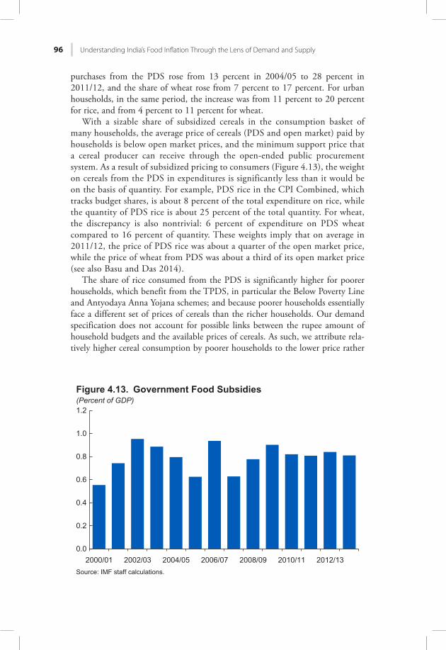
With a sizable share of subsidized cereals in the consumption basket of many households, the average price of cereals (PDS and open market) paid by households is below open market prices, and the minimum support price that a cereal producer can receive through the open-ended public procurement system. As a result of subsidized pricing to consumers (Figure 4.13), the weight on cereals from the PDS in expenditures is significantly less than it would be on the basis of quantity. For example, PDS rice in the CPI Combined, which tracks budget shares, is about 8 percent of the total expenditure on rice, while the quantity of PDS rice is about 25 percent of the total quantity. For wheat, the discrepancy is also nontrivial: 6 percent of expenditure on PDS wheat compared to 16 percent of quantity. These weights imply that on average in 2011/12, the price of PDS rice was about a quarter of the open market price, while the price of wheat from PDS was about a third of its open market price (see also Basu and Das 2014).
The share of rice consumed from the PDS is significantly higher for poorer households, which benefit from the TPDS, in particular the Below Poverty Line and Antyodaya Anna Yojana schemes; and because poorer households essentially face a different set of prices of cereals than the richer households. Our demand specification does not account for possible links between the rupee amount of household budgets and the available prices of cereals. As such, we attribute rela-tively higher cereal consumption by poorer households to the lower price rather
0.0
0.2
0.4
0.6
0.8
1.0
1.2
2000/01 2002/03 2004/05 2006/07 2008/09 2010/11 2012/13Source: IMF staff calculations.
Figure 4.13. Government Food Subsidies(Percent of GDP)
Anand, Kumar, and Tulin 97
than to their smaller budgets.8 In other words, the estimated demand system is conditional on the distribution of cereal prices with respect to the level of house-hold budget, which in practice is ensured through the in-kind nature of the TPDS. Moreover, it does not account for leakages, which are estimated to be large (CACP 2013). As a result, our estimated demand system may not be fully captur-ing the effects of these distortions, and is only suitable to study demand under the existing food distribution policy and associated subsidies.
BUFFER STOCKS AND MINIMUM SUPPORT PRICESBuffer Stocks
In this section, we quantify the impact of the buildup of buffer stocks on India’s relative food inflation over the past decade. Specifically, we estimate relative food inflation because of the diminished net supply of cereals into the market from the buildup of buffer stocks. We also estimate the impact of a hypothetical (and counterfactual) proactive buffer stock liquidation policy on relative food inflation volatility.
It has been frequently argued that the excessive buildup of buffer stocks for cereals (rice and wheat) contributed to India’s inflationary pressures in the past several years (CACP 2013). The cumulative buildup of the buffer stock of rice over a six-year period from 2007/08 to 2012/13 was close to 20 million tons, while average production was about 100 million tons. The buildup of wheat stocks was even more significant; the average wheat stock in the Central Pool during 2012/13 exceeded average stocks in 2007/08 by about 30 million tons, as production averaged 85 million tons per year. The rice intake into the Central Pool averaged 4 percent of annual output during this period, and nearly 7 percent for wheat. As a result, by July 2012, India’s stocks of rice and wheat accounted for more than 6 percent and 7 percent of the world’s total rice and wheat utilization, respectively (Saini and Kozicka 2014). Since 2010, on aver-age, actual buffer stocks held with the Food Corporation of India were more than double the norms. Several underlying reasons account for this situation, including distortions such as export bans and open-ended procurement. But a key reason appears to be lack of a proactive liquidation policy. The inefficiency of the buffer stock policy has been aggravated by the significant costs of carry-ing excess stocks, considering that the economic cost to the Food Corporation of India for acquiring, storing, and distributing food grains has been some 40–50 percent more than the procurement prices (Gulati, Gujral, and Nandakumar 2012).
In practice, minimum support price increases are announced in advance of the agricultural season, the actual intake to buffer stock following harvesting has a
8 For example, the bottom decile of rural households have a budget share of cereals of about one-fourth, and it declines to less than one-tenth for the top decile. In urban India, the share of cereals falls from slightly less than one-fifth to just 3–4 percent for the top decile households.
98 Understanding India’s Food Inflation Through the Lens of Demand and Supply
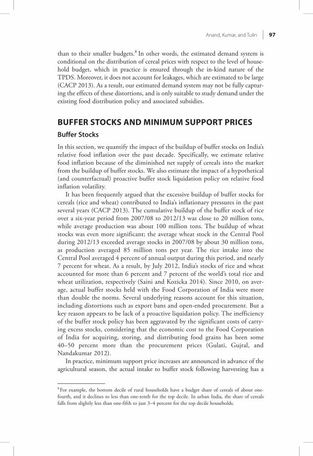
further impact on inflation dynamics, because it reduces the quantity of cereals available for households’ purchases on the open market, especially during a poor output period. Even though minimum support prices essentially provide a floor for open market prices, in part due to an open-ended procurement policy, the actual postharvest buffer stock intake and household demand define the eventual open market prices. Figure 4.14 illustrates a simplified interaction of postharvest short-term supply and demand for cereals. If we abstract away from international trade aspects, we can assume that the postharvest short-term cereal supply curve is vertical. In addition, we assume that the government’s decision on the buildup of buffer stocks does not depend on the price paid, which implies a vertical gov-ernment demand curve. The increase in government demand for buffer stock buildup leads to a parallel rightward shift of the total cereal demand curve. Under these assumptions of fixed supply and fixed government demand, the quantity available for households’ open market purchases is reduced by a fixed amount, implying that the inflationary impact of buffer stock intake can be assessed solely using the structure of household demand.
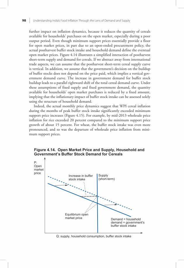
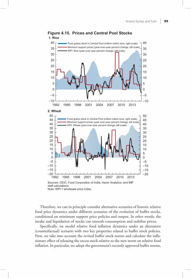
Indeed, the actual monthly price dynamics suggest that WPI cereal inflation during the months of peak buffer stock intake significantly exceeded minimum support price increases (Figure 4.15). For example, by mid-2013 wholesale price inflation for rice exceeded 20 percent compared to the minimum support price growth of about 15 percent. For wheat, the buffer stock intake was even more pronounced, and so was the departure of wholesale price inflation from mini-mum support prices.
Demand = householddemand + government’s buffer stock intake
Q: supply, household consumption, buffer stock intake
Equilibrium open market price
P:Openmarketprice
Figure 4.14. Open Market Price and Supply, Household andGovernment’s Buffer Stock Demand for Cereals
Increase in bufferstock intake
Supply(short-term)
Anand, Kumar, and Tulin 99
Therefore, we can in principle consider alternative scenarios of historic relative food price dynamics under different scenarios of the evolution of buffer stocks, conditional on minimum support price policies and output. In other words, the intake and liquidation of stocks can smooth consumption and stabilize prices.
Specifically, we model relative food inflation dynamics under an alternative (counterfactual) scenario with two key properties related to buffer stock policies. First, we take into account the revised buffer stock norms and calculate the infla-tionary effect of releasing the excess stock relative to the new norm on relative food inflation. In particular, we adopt the government’s recently approved buffer norms,
2. Wheat
–10
–5
0
5
10
15
20
25
30
35
40
–10
–5
0
5
10
15
20
25
30
35
40
1992 1995 1998 2001 2004 2007 2010 2013
Food grains stock in Central Pool (million metric tons, right scale)Minimum support prices (year-over-year percent change, left scale)WPI: Rice (year-over-year percent change, left scale)
–20–15–10–505101520253035404550
–20–15–10
–505
101520253035404550
1992 1995 1998 2001 2004 2007 2010 2013
Food grains stock in Central Pool (million metric tons, right scale)Minimum support prices (year-over-year percent change, left scale)WPI: Wheat (year-over-year percent change, left scale)
Sources: CEIC; Food Corporation of India; Haver Analytics; and IMFstaff calculations.Note: WPI = wholesale price index.
Figure 4.15. Prices and Central Pool Stocks 1. Rice
100 Understanding India’s Food Inflation Through the Lens of Demand and Supply
reflecting the needs of the National Food Security Act.9 Our scenario analysis has a reduced net overall buffer stock intake between 2006/07 and 2013/14 that results in average stocks in the Central Pool during 2013/14 reaching close to the revised norm levels. More specifically, we assume a lower cumulative buffer stock intake between July 2007 and July 2012, by about 15 million metric tons for rice and by about 20 million metric tons for wheat. Our estimates suggest that this would have resulted in a reduction in food inflation by about ½ percentage point per year compared to the actual aggregate stock intake during 2006/07–2012/13, assuming the government had continued to subsidize PDS distribution of cereals.
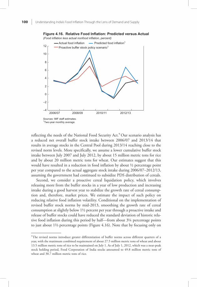
Second, we consider a proactive cereal liquidation policy, which involves releasing more from the buffer stocks in a year of low production and increasing intake during a good harvest year to stabilize the growth rate of cereal consump-tion and, therefore, market prices. We estimate the impact of such policy on reducing relative food inflation volatility. Conditional on the implementation of revised buffer stock norms by mid-2013, smoothing the growth rate of cereal consumption at slightly below 1½ percent per year through a proactive intake and release of buffer stocks could have reduced the standard deviation of historic rela-tive food inflation during this period by half—from about 3¼ percentage points to just about 1⅔ percentage points (Figure 4.16). Note that by focusing only on
9 The revised norms introduce greater differentiation of buffer norms across different quarters of a year, with the maximum combined requirement of about 27.5 million metric tons of wheat and about 13.5 million metric tons of rice to be maintained on July 1. As of July 1, 2012, which was a near-peak stock holding period, Food Corporation of India stocks amounted to 49.8 million metric tons of wheat and 30.7 million metric tons of rice.
Hkiwtg"60380 Tgncvkxg"Hqqf"Kphncvkqp<"Rtgfkevgf"xgtuwu"Cevwcn(Food inflation less actual nonfood inflation, percent)
Sources: IMF staff estimates.1Two-year monthly average.
–4
–2
0
2
4
6
8
10
12
2006/07 2008/09 2010/11 2012/13
Actual food inflation Predicted food inflation1
Proactive buffer stock policy scenario1
Anand, Kumar, and Tulin 101
modeling the relative food inflation and keeping the path of nonfood inflation unchanged, we ignore potential second-round effects of elevated food inflation on core inflation, which are nontrivial (Anand, Ding, and Tulin 2014). Therefore, our exercise likely understates the additional impact on aggregate retail inflation, particularly at times of elevated food inflation.
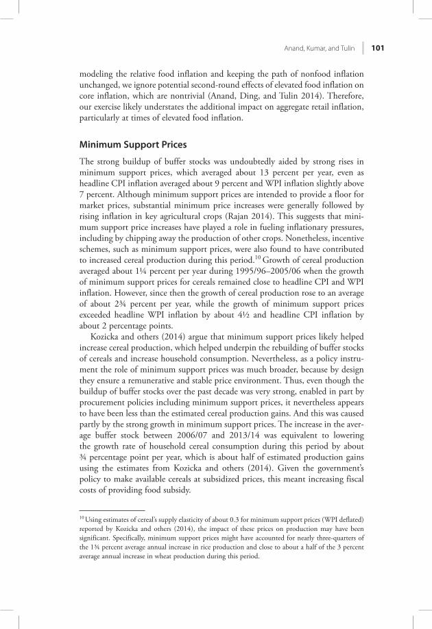
Minimum Support Prices
The strong buildup of buffer stocks was undoubtedly aided by strong rises in minimum support prices, which averaged about 13 percent per year, even as headline CPI inflation averaged about 9 percent and WPI inflation slightly above 7 percent. Although minimum support prices are intended to provide a floor for market prices, substantial minimum price increases were generally followed by rising inflation in key agricultural crops (Rajan 2014). This suggests that mini-mum support price increases have played a role in fueling inflationary pressures, including by chipping away the production of other crops. Nonetheless, incentive schemes, such as minimum support prices, were also found to have contributed to increased cereal production during this period.10 Growth of cereal production averaged about 1¼ percent per year during 1995/96–2005/06 when the growth of minimum support prices for cereals remained close to headline CPI and WPI inflation. However, since then the growth of cereal production rose to an average of about 2¾ percent per year, while the growth of minimum support prices exceeded headline WPI inflation by about 4½ and headline CPI inflation by about 2 percentage points.
Kozicka and others (2014) argue that minimum support prices likely helped increase cereal production, which helped underpin the rebuilding of buffer stocks of cereals and increase household consumption. Nevertheless, as a policy instru-ment the role of minimum support prices was much broader, because by design they ensure a remunerative and stable price environment. Thus, even though the buildup of buffer stocks over the past decade was very strong, enabled in part by procurement policies including minimum support prices, it nevertheless appears to have been less than the estimated cereal production gains. And this was caused partly by the strong growth in minimum support prices. The increase in the aver-age buffer stock between 2006/07 and 2013/14 was equivalent to lowering the growth rate of household cereal consumption during this period by about ¾ percentage point per year, which is about half of estimated production gains using the estimates from Kozicka and others (2014). Given the government’s policy to make available cereals at subsidized prices, this meant increasing fiscal costs of providing food subsidy.
10 Using estimates of cereal’s supply elasticity of about 0.3 for minimum support prices (WPI deflated) reported by Kozicka and others (2014), the impact of these prices on production may have been significant. Specifically, minimum support prices might have accounted for nearly three-quarters of the 1¾ percent average annual increase in rice production and close to about a half of the 3 percent average annual increase in wheat production during this period.
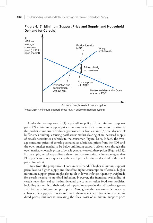
102 Understanding India’s Food Inflation Through the Lens of Demand and Supply
Under the assumptions of (1) a price-floor policy of the minimum support price, (2) minimum support prices resulting in increased production relative to the market equilibrium without government subsidies, and (3) the absence of buffer stock buildup, ensuring postharvest market clearing of an increased supply of cereals necessitates a subsidy to the consumer (Figure 4.17). Indeed, the aver-age consumer prices of cereals purchased at subsidized prices from the PDS and the open market tended to be below minimum support prices, even though the open market wholesale prices of cereals generally exceed these prices (Figure 4.18). For example, cereal expenditure shares and consumption volumes suggest that PDS prices are about a quarter of the retail prices for rice, and a third of the retail prices for wheat.
Thus, from the perspective of consumer demand, if higher minimum support prices lead to higher supply and therefore higher consumption of cereals, higher minimum support prices might also result in lower inflation (quantity weighted) for cereals relative to nonfood inflation. However, the increased availability of cereals may also lead to further demand pressures on other food commodities, including as a result of their reduced supply due to production distortions gener-ated by the minimum support price. Also, given the government’s policy to enhance the supply of cereals and make them available to households at subsi-dized prices, this means increasing the fiscal costs of minimum support price
Supply(preharvest)
Q: production, household consumption
Figure 4.17. Minimum Support Price and Supply, and Household Demand for Cereals
Production withMSP
Price subsidyto consumer
Consumption with MSP
P:MSP and average consumer price (PDS + open market)
Production and consumption without MSP Household demand = Open
market + PDS
Note: MSP = minimum support price; PDS = public distribution system.
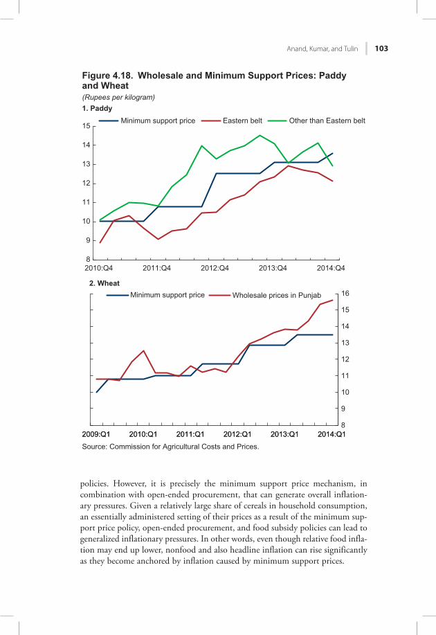
Anand, Kumar, and Tulin 103
policies. However, it is precisely the minimum support price mechanism, in combination with open-ended procurement, that can generate overall inflation-ary pressures. Given a relatively large share of cereals in household consumption, an essentially administered setting of their prices as a result of the minimum sup-port price policy, open-ended procurement, and food subsidy policies can lead to generalized inflationary pressures. In other words, even though relative food infla-tion may end up lower, nonfood and also headline inflation can rise significantly as they become anchored by inflation caused by minimum support prices.
8
9
10
11
12
13
14
15
2010:Q4 2011:Q4 2012:Q4 2013:Q4 2014:Q4
Minimum support price Eastern belt Other than Eastern belt
8
9
10
11
12
13
14
15
16
2009:Q1 2010:Q1 2011:Q1 2012:Q1 2013:Q1 2014:Q12009:Q1
Source: Commission for Agricultural Costs and Prices.
2010:Q1 2011:Q1 2012:Q1 2013:Q1 2014:Q1
Minimum support price Wholesale prices in Punjab2. Wheat
Figure 4.18. Wholesale and Minimum Support Prices: Paddyand Wheat(Rupees per kilogram)1. Paddy
104 Understanding India’s Food Inflation Through the Lens of Demand and Supply
Note that our simulation framework is aimed at explaining relative food infla-tion for a given level of nonfood inflation rather than establishing a causal rela-tionship. A possible simulation approach, of course, could be to tie food and nonfood prices to administered prices, such as the minimum support price, and then solve for inflation dynamics conditional on cereal price inflation. It is not clear to what extent this is a useful exercise because, while not trivial, products subject to minimum support prices constitute a relatively small share of total consumption. In this case, time-series techniques aimed at identifying causal links may be better suited, as examined in Sonna and others (2014), for example. Controlling for real incomes, demand for protein, and agricultural input costs, they find that a 1 percentage point increase in the production-weighted mini-mum support price of rice and wheat is associated with about a 0.3 percentage point increase in food inflation. In addition, on the basis of weak exogeneity tests, they conclude that in the short-term, minimum support prices have a statistically significant impact on food inflation. Similarly, Anand, Ding, and Tulin (2014), using a reduced-form dynamic general equilibrium model for India, show that food inflation shocks can lead to a significant increase in core inflation.
Finally, empirical evidence provided by Anand, Kumar, and Tulin (2016) sug-gests that, except in the short term, minimum support prices of cereals tend to react to changes in Indian farm gate prices of cereals, rather than the other way around. They also find that international market prices influence Indian farm gate prices and minimum support prices, in both the short and long term. The global market price will thus remain important in defining Indian cereal prices in the long term.
IMPLICATIONS FOR MONETARY POLICYOur modeling framework does not take into account that supply could be responsive to prices. By imposing adjustment only on prices and demand, it may not be ideal to study situations when supply is price elastic. And it may be par-ticularly limiting when analyzing long-term food inflation dynamics.
As discussed, the approach of abstracting away from explicit modeling of food supply is not without limitations,11 and the estimated inflation outcomes are likely to have an upward bias. Nonetheless, as own-price supply elasticities are usually found to be significantly below demand elasticities, responsiveness of supply to mitigate the impact of demand on prices may be rather limited, particularly over the near term. The Food and Agricultural Policy Research Institute’s Elasticity Database, for example, indicates that the price elasticities of rice supply are usually close to 0.2, with a value of 0.25 in Bangladesh, 0.16 in China, and 0.11 in India. The price elasticities of response for wheat are slightly higher, averaging, for example, 0.33 in Australia, 0.43 in Brazil, 0.09 in China, and 0.29 in India. In the case of more recent studies on India, Kumar and others (2010) report similar estimates of own-price elasticities of supply: 0.24 for rice, 0.22 for wheat, and 0.17 for pulses. Supply elasticities for minimum support prices, estimated by Kozicka
11 As in an inelastic supply system, only price, not supply, adjusts to equilibrate demand.
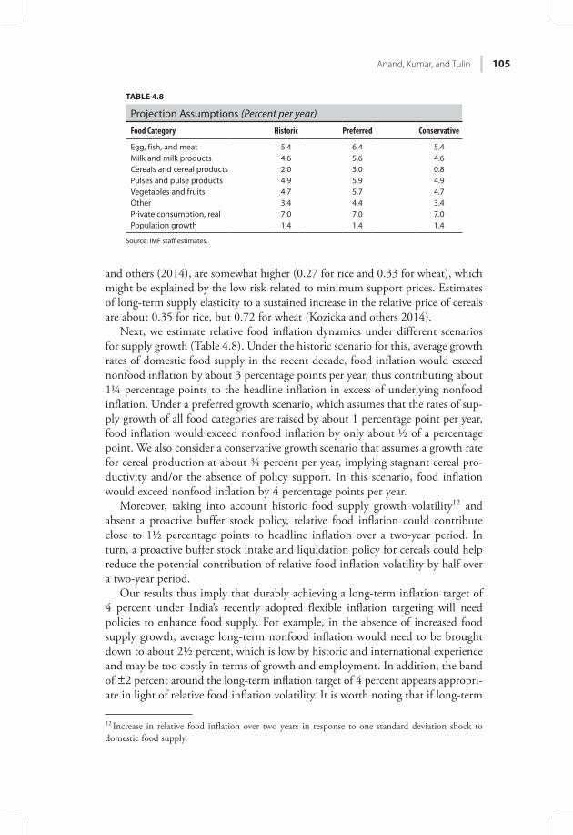
Anand, Kumar, and Tulin 105
and others (2014), are somewhat higher (0.27 for rice and 0.33 for wheat), which might be explained by the low risk related to minimum support prices. Estimates of long-term supply elasticity to a sustained increase in the relative price of cereals are about 0.35 for rice, but 0.72 for wheat (Kozicka and others 2014).
Next, we estimate relative food inflation dynamics under different scenarios for supply growth (Table 4.8). Under the historic scenario for this, average growth rates of domestic food supply in the recent decade, food inflation would exceed nonfood inflation by about 3 percentage points per year, thus contributing about 1¼ percentage points to the headline inflation in excess of underlying nonfood inflation. Under a preferred growth scenario, which assumes that the rates of sup-ply growth of all food categories are raised by about 1 percentage point per year, food inflation would exceed nonfood inflation by only about ½ of a percentage point. We also consider a conservative growth scenario that assumes a growth rate for cereal production at about ¾ percent per year, implying stagnant cereal pro-ductivity and/or the absence of policy support. In this scenario, food inflation would exceed nonfood inflation by 4 percentage points per year.
Moreover, taking into account historic food supply growth volatility12 and absent a proactive buffer stock policy, relative food inflation could contribute close to 1½ percentage points to headline inflation over a two-year period. In turn, a proactive buffer stock intake and liquidation policy for cereals could help reduce the potential contribution of relative food inflation volatility by half over a two-year period.
Our results thus imply that durably achieving a long-term inflation target of 4 percent under India’s recently adopted flexible inflation targeting will need policies to enhance food supply. For example, in the absence of increased food supply growth, average long-term nonfood inflation would need to be brought down to about 2½ percent, which is low by historic and international experience and may be too costly in terms of growth and employment. In addition, the band of ±2 percent around the long-term inflation target of 4 percent appears appropri-ate in light of relative food inflation volatility. It is worth noting that if long-term
12 Increase in relative food inflation over two years in response to one standard deviation shock to domestic food supply.
TABLE 4.8
Projection Assumptions (Percent per year)
Food Category Historic Preferred Conservative
Egg, fish, and meat 5.4 6.4 5.4Milk and milk products 4.6 5.6 4.6Cereals and cereal products 2.0 3.0 0.8Pulses and pulse products 4.9 5.9 4.9Vegetables and fruits 4.7 5.7 4.7Other 3.4 4.4 3.4Private consumption, real 7.0 7.0 7.0Population growth 1.4 1.4 1.4
Source: IMF staff estimates.
106 Understanding India’s Food Inflation Through the Lens of Demand and Supply
average inflation were higher, the upper band would probably be breached more often or would need a more aggressive monetary stance. Our analysis also suggests that administered price setting, such as through minimum support prices and supporting policies, constitute an important impediment to monetary policy transmission and will continue to pose challenges for monetary policy manage-ment in India. Finally, a proactive buffer stock policy could be instrumental in containing inflation volatility and limiting the burden on monetary policy in addressing the adverse consequences of food supply shocks, including the second-round effects of food inflation shocks to core inflation.
CONCLUSIONS AND POLICY IMPLICATIONSDuring the decade just past, India has seen a prolonged period of high inflation, to a large extent driven by persistently high food inflation. Domestic food demand and supply factors underpin India’s food price dynamics. Relative food prices have played a key role in equilibrating India’s food demand and domestic supply, given the limited responsiveness of agricultural production, particularly in the short term. The acceleration of India’s economic growth during the past 10 years, accompanied by stagnant agriculture growth, resulted in excess demand for food, giving rise to relative food price inflation. Furthermore, the excessive buildup in buffer stocks since 2007/08 and the lack of a proactive liquidation policy increased average relative food inflation and its volatility.
As India’s economic growth picks up, food demand pressures will remain strong, particularly for high-value foods, such as dairy products and animal-based proteins. Rising incomes will prompt shifts in food consumption away from simple starchy plant–dominated diets toward more nutritious and high-value foods. Recent steps to contain food inflation will help in the short term, until durable measures to increase food supply are put in place. The recent measures to limit the rise of minimum support prices for key agricultural commodities, wheat and rice in particular; the release of food grains from the Central Pool into the market; and adjusting the buffer norms of food grains to levels significantly below prevailing actual stocks have helped lower cereal (rice and wheat) inflation. However, India’s agricultural yields for key food commodities remain significantly below those of many emerging markets; rice yields, for example, are about one-third of China’s and about half of Vietnam’s and Indonesia’s (Himani 2014). The excess demand will likely reemerge; and thus a durable increase in supply, par-ticularly through enhancing agricultural yields for key commodities, will be required to keep food inflation in check. For cereals, the impact of price support and stabilization policies will need to be complemented by policies to enhance agricultural productivity, including along the lines of the FCI Restructuring Committee Report (Government of India 2015).
In the absence of a stronger food supply growth response, relative food infla-tion can contribute about 1¼ percentage points to headline inflation annually. Indian food inflation is likely to exceed nonfood inflation by 2½–3 percentage points per year, assuming private consumption growth picking up to 7 percent
Anand, Kumar, and Tulin 107
per year and food supply growing at historic rates. Therefore, the sustainability of a long-term inflation target of 4 percent under the recently adopted flexible infla-tion targeting will depend on enhancing food supply, agricultural market-based pricing, and reducing price distortions. In the interim, monetary policy will need to remain tight to anchor inflation expectations at a lower level. Our simulation analysis also indicates that in light of India’s supply-side vulnerabilities, the band around the inflation target of ±2 percent is broadly appropriate. A well-designed cereal buffer stock liquidation policy could help mitigate food inflation volatility. Finally, administered price setting, such as through minimum support prices and supporting policies, will continue to pose challenges for monetary policy manage-ment in India, as highlighted in the Patel Committee Report.
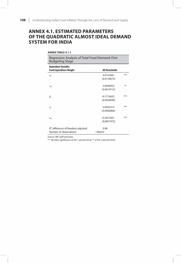
108 Understanding India’s Food Inflation Through the Lens of Demand and Supply
ANNEX 4.1. ESTIMATED PARAMETERS OF THE QUADRATIC ALMOST IDEAL DEMAND SYSTEM FOR INDIA
ANNEX TABLE 4.1.1
Regression Analysis of Total Food Demand: First Budgeting Stage
Dependent Variable: Food Expenditure Weight All Households
af 0.9147661 ***(0.0139673)
gf,f 0.0040952 **(0.0019713)
bf –0.1710632 ***(0.0030094)
lf 0.0035315 ***(0.0002866)
a0 –0.3615261 ***(0.0871973)
R², difference of freedom adjusted 0.96Number of observations 138,055
Source: IMF staff estimates.*** denotes significance at the 1 percent level; ** at the 5 percent level.
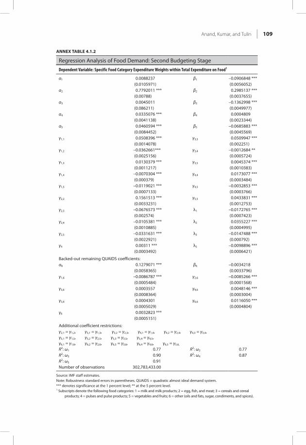
Anand, Kumar, and Tulin 109
ANNEX TABLE 4.1.2
Regression Analysis of Food Demand: Second Budgeting Stage
Dependent Variable: Specific Food Category Expenditure Weights within Total Expenditure on Food1
α1 0.0088237 β1 –0.0906848 ***(0.0105971) (0.0056052)
α2 0.7792011 *** β2 0.2985137 ***(0.00788) (0.0037655)
α3 0.0045011 β3 –0.1362998 ***(0.086211) (0.0049977)
α4 0.0335076 *** β4 0.0004809(0.0041138) (0.0023344)
α5 0.0460594 *** β5 –0.0685883 ***(0.0084452) (0.0045569)
γ1,1 0.0508396 *** γ3,3 0.0509947 ***(0.0014078) (0.002251)
γ1,2 –0.0362661*** γ3,4 –0.0012684 **(0.0025156) (0.0005724)
γ1,3 0.0130379 *** γ3,5 0.0045374 ***(0.0011217) (0.0010383)
γ1,4 –0.0070304 *** γ4,4 0.0173077 ***(0.000379) (0.0003484)
γ1,5 –0.0119021 *** γ4,5 –0.0032853 ***(0.0007133) (0.0003766)
γ2,2 0.1561513 *** γ5,5 0.0433831 ***(0.0033231) (0.0012753)
γ2,3 –0.0676573 *** λ1 –0.0172765 ***(0.002574) (0.0007423)
γ2,4 –0.0105381 *** λ2 0.0355227 ***(0.0010885) (0.0004995)
γ2,5 –0.0331631 *** λ3 –0.0147488 ***(0.0022921) (0.000792)
γ4 0.00311 *** λ5 –0.0098896 ***(0.0003492) (0.0006421)
Backed-out remaining QUAIDS coefficients:α6 0.1279071 *** β6 –0.0034218
(0.0058365) (0.0033796)γ1,6 –0.0086787 *** γ2,6 –0.0085266 ***
(0.0005484) (0.0001568)γ3,6 0.0003557 γ4,6 0.0048146 ***
(0.0008364) (0.0003004)γ5,6 0.0004301 γ6,6 0.0116050 ***
(0.0005029) (0.0004804)γ6 0.0032823 ***
(0.0005151)
Additional coefficient restrictions:γ2,1 = γ1,2, γ3,1 = γ1,3, γ3,2 = γ2,3, γ4,1 = γ1,4, γ4,2 = γ2,4, γ4,3 = γ3,4, γ5,1 = γ1,5, γ5,2 = γ2,5, γ5,3 = γ3,5, γ5,4 = γ4,5, γ6,1 = γ1,6, γ6,2 = γ2,6, γ6,3 = γ3,6, γ6,4 = γ4,6, γ6,5 = γ5,6,
R2: ω1 0.77 R2: ω2 0.77R2: ω3 0.90 R2: ω4 0.87R2: ω5 0.91Number of observations 302,783,433.00
Source: IMF staff estimates.Note: Robustness standard errors in parentheses. QUAIDS = quadratic almost ideal demand system.*** denotes significance at the 1 percent level; ** at the 5 percent level.1 Subscripts denote the following food categories: 1 = milk and milk products; 2 = egg, fish, and meat; 3 = cereals and cereal
products; 4 = pulses and pulse products; 5 = vegetables and fruits; 6 = other (oils and fats, sugar, condiments, and spices).
110 Understanding India’s Food Inflation Through the Lens of Demand and Supply
REFERENCESAnand, Rahul, Ding Ding, and Volodymyr Tulin. 2014. “Food Inflation in India: The Role for
Monetary Policy.” IMF Working Paper 14/178, International Monetary Fund, Washington.Anand, Rahul, Naresh Kumar, and Volodymyr Tulin. 2016. “Understanding India’s Food
Inflation: The Role of Demand and Supply Factors.” IMF Working Paper 16/2, International Monetary Fund, Washington.
Basu, Deepankar, and Debarshi Das. 2014. “Social Hierarchies and Public Distribution of Food in Rural India.” Working Paper 2014–05, University of Massachusetts Amherst, Massachusetts.
Banks, James, Richard Blundell, and Arthur Lewbel. 1997. “Quadratic Engel Curves and Consumer Demand.” Review of Economics and Statistics 69 (4): 527–39.
Beatty, Timothy, and Erling Larsen. 2005. “Using Engel Curves to Estimate Bias in the Canadian CPI as a Cost of Living Index.” Canadian Journal of Economics, 38 (2): 482–99.
Blanciforti, Laura, and Richard Green. 1983. “An Almost Ideal Demand System Incorporating Habits: An Analysis of Expenditures on Food and Aggregate Community Groups.” Review of Economics and Statistics 65 (3): 511–15.
Blundell, Richard, Alan Duncan, and Krishna Pendakur. 1998. “Semiparametric Estimation and Consumer Demand.” Journal of Applied Econometrics 13 (5): 435–61.
Commission for Agricultural Costs and Prices (CACP), Government of India. 2013. “Price Policy for Kharif Crops. The Marketing Season 2013–14.” Kharif Price Policy Reports. March.
Deaton, Angus S., and John Muellbauer. 1980. “An Almost Ideal Demand System.” American Economic Review 70 (3): 312–26.
Ganesh-Kumar A., Rajesh Mehta, Hemant Pullabhotla, Sanjay K. Prasad, Kavery Ganguly, and Ashok Gulati. 2012. “Demand and Supply of Cereals in India, 2010–2025.” Discussion Paper 01158, International Food Policy Research Institute, Washington.
Gokarn, Subir. 2011. “Food Inflation—This Time It’s Different.” Kale Memorial Lecture, Gokhale Institute of Politics and Economics, Pune, December 9.
Government of India. 2015. “Reorienting the Role and Restructuring of Food Corporation of India.” Report of the High Level Committee, New Delhi.
Gulati, Ashok, Jyoti Gujral, and T. Nandakumar. 2012. “National Food Security Bill, Challenges and Options.” Discussion Paper 2, Commission on Agricultural Costs and Prices, New Delhi.
Himani. 2014. “An Analysis of Agricultural Sector in Indian Economy.” Journal of Humanities and Social Science, 19 (1): 47–57.
Kozicka, Marta, Matthias Kalkuhl, Shweta Saini, and Jan Brockhaus. 2014. “Modeling Indian Wheat and Rice Sector Policies.” Paper presented at the Agricultural and Applied Economics Association annual meeting, Minneapolis, July 27–29.
Kumar, Praduman, P. Shinoj, S. S. Raju, Anjani Kumar, Karl M. Rich, and Siwa Msangi. 2010. “Factor Demand, Output Supply Elasticities and Supply Projections for Major Crops in India.” Agricultural Economics Research Review 23 (January–June): 1–14.
International Monetary Fund (IMF). 2011. “India: 2010 Article IV Consultation.” IMF Country Report 11/50, Washington.
———. 2012. “India: 2012 Article IV Consultation.” IMF Country Report 12/96, Washington.
———. 2013. “India: 2013 Article IV Consultation.” IMF Country Report 13/37, Washington.
———. 2014a. “India: 2014 Article IV Consultation.” IMF Country Report 14/57, Washington.
———. 2014b. “India: Selected Issues.” IMF Country Report 14/58, Washington.Leser, Conrad. 1963. “Forms of Engel Functions.” Econometrica 31: 694–703.Mohan, Rakesh, and Muneesh Kapur. 2015. “Pressing the Indian Growth Accelerator: Policy
Imperatives.” IMF Working Paper 15/53, International Monetary Fund, Washington.
Anand, Kumar, and Tulin 111
Organisation for Economic Co-operation and Development (OECD). 2009. Agricultural Policies in Emerging Economies 2009: Monitoring and Evaluation. Paris: OECD.
Poi, Brian P. 2002. “From the Help Desk: Demand System Estimation.” Stata Journal 2 (4): 403–10.
———. 2008, “Demand-System Estimation: Update.” Stata Journal 8 (4): 554–56.Rajan, Raghuram. 2014. “Fighting Inflation.” Speech at the FIMMDA-PDAI annual confer-
ence, Mumbai, February 26.Reserve Bank of India (RBI). 2014a. Report of the Expert Committee to Revise and Strengthen the
Monetary Policy Framework. Mumbai: RBI. http://rbidocs.rbi.org.in/rdocs/PublicationReport/Pdfs/ECOMRF210114_F.pdf.
———. 2014b. Reserve Bank of India Annual Report 2013–14. Mumbai: RBI.Saini, Shweta, and Marta Kozicka. 2014. “Evolution and Critique of Buffer Stocking Policy of
India.” ICRIER Working Paper 283, Indian Council for Research on International Economic Relations, New Delhi.
Sonna, Thangzason, Himanshu Joshi, Alice Sebastian, and Upasana Sharma. 2014. “Analytics of Food Inflation in India.” RBI Working Paper Series 10, Reserve Bank of India, Mumbai.
Walsh, James P. 2011. “Reconsidering the Role of Food Prices in Inflation.” IMF Working Paper 11/71, International Monetary Fund, Washington.
Yatchew, Adonis. 2003. Semiparametric Regression for the Applied Econometrician. Cambridge: Cambridge University Press.

223
CONTRIBUTORS
Rahul Anand is Assistant to the Director in the IMF’s Institute for Capacity Development. Prior to this, he worked in the African Department and the Asia and Pacific Department, covering South Africa, India, and Sri Lanka. His research spans a range of areas, including general equilibrium modeling to study monetary policy issues in emerging markets, macro-critical structural reforms, subsidy reforms, and growth-enhancing structural transformation. He has pub-lished widely, including in the Journal of Monetary Economics, and his research has also featured in The Economist, the Financial Times, and the Wall Street Journal. Before joining the IMF in 2010, he held various senior positions in India as a member of the Indian Administrative Service—designing, implementing, and monitoring government economic programs and policies. He has a PhD from Cornell University and a master’s degree from Harvard University.
Paul Cashin is Assistant Director in the Asia and Pacific Department and Mission Chief for India. Prior to this, he worked in the IMF’s Research Department, on issues related to developing countries; in the IMF’s Western Hemisphere Department, where he was Chief of the Caribbean Division and Mission Chief to the Eastern Caribbean Currency Union, St. Lucia, and St. Vincent; and in the Middle East and Central Asia Department, where he was Chief of the Regional Studies Division and Mission Chief to Jordan. Before join-ing the IMF, Mr. Cashin was Principal Research Economist at the Ministry of Agriculture in Victoria, Australia, and Associate Professor in the Department of Economics at the University of Melbourne, Australia. Mr. Cashin has published widely in several fields of economics, including macroeconomic modeling, com-modity prices and exchange rates, international economics, and economic devel-opment. He obtained his PhD and an MA in Economics from Yale University, and holds an MAgrSc in Agricultural Economics and a bachelor’s degree in Economics from the University of Melbourne in Australia.
Sonali Das is an Economist in the IMF’s Asia and Pacific Department, covering India and Nepal. Prior to this, she was in the IMF’s Strategy, Policy, and Review Department, where her responsibilities included working on the IMF program with Pakistan. Ms. Das received her PhD in Economics from Cornell University in 2012 and holds an MA from McGill University and a BSc from the University of Toronto. During the course of her doctoral studies she was a visiting fellow at the Federal Reserve Bank of San Francisco, a research associate at the Brookings Institution, and a summer intern at the IMF. Her research interests include bank-ing, financial stability, and financial development.
Roberto Guimarães is a Deputy Division Chief in the Regional Studies Division of the IMF’s Asia and Pacific Department. He has worked on a number of countries,
224 Contributors
including covering financial sector issues in Mexico and Argentina, and on IMF surveillance teams covering India, Malaysia, Singapore, Costa Rica, and Panama. He has also led IMF missions to Bhutan and Fiji. Mr. Guimarães has published in Economics Letters, Economics Bulletin, Applied Financial Economics, Finance & Development, as well as IMF working papers and Occasional Papers. He has worked on a range of policy issues in international finance and macroeconomics, including capital flows, foreign exchange intervention, and monetary policy. He holds a PhD in economics and an MSc in Statistics.
Naresh Kumar is currently a Research Analyst in the IMF’s African Department. Previously, he worked on India at the IMF office in Delhi and on Latin American countries while in the private sector. He joined the IMF in 2009. He is an Indian national and has a master’s and a bachelor’s degree in Economics from Delhi University. He has published on growth and inequality, labor market issues, and inflation in India. His research interests are in monetary policy in low-income countries, trade, structural issues, inequality, and labor market issues.
Kamiar Mohaddes is a Senior Lecturer and Fellow in Economics at Girton College, University of Cambridge. He is also a member of the Economic Research Forum (ERF) advisory committee, an ERF Research Fellow, and an associate researcher at the Energy Policy Research Group (EPRG), University of Cambridge. He holds a BSc in Economics from the University of Warwick and an MPhil and a PhD in Economics from the University of Cambridge. His main areas of research are macroeconomics, global and national macroeconometric modeling, and energy economics. His articles have been published in a number of edited volumes (Cambridge University Press and Routledge) as well as in leading jour-nals, including the Journal of Applied Econometrics and Energy Economics.
Adil Mohommad joined the IMF as an Economist in 2011. He currently works in the Asia Pacific Department on Australia and New Zealand, and previously also worked on Nepal and Bhutan. His research includes work on trade, institutions, productivity, and growth. He received his BA from Delhi University, MA from Delhi School of Economics, and his PhD from the University of Maryland in 2010.
Prachi Mishra is on leave from the IMF as Specialist Adviser (equivalent to Chief General Manager) in the Department of Economic and Policy Research at the Reserve Bank of India. Prior to that, she was Senior Economist in the Office of Chief Economic Advisor in the Ministry of Finance, and at the Prime Minister’s Economic Advisory Council in the Government of India; and Senior Economist at the IMF. At the IMF, she has worked for the Monetary and Capital Markets, Research, Western Hemisphere, and Fiscal Affairs Departments, and in the office of the First Deputy Managing Director. She received a PhD in Economics from Columbia University in 2004, and a master’s degree from the Delhi School of Economics in 1999.
Yasuhisa Ojima is a Senior Economist in the Asia and Pacific Department and a Mission Chief for Tonga. Prior to joining the IMF, he was a Director in the
Contributors 225
Credit Risk Analysis division at the Japan International Cooperation Agency (JICA) and a Resident Representative for the Japan Bank for International Cooperation (JBIC) in Vietnam. He has published several textbooks and articles in the field of international and development economics and taught at Waseda University in Tokyo. Mr. Ojima holds degrees from Yale University and Keio University.
Laura Papi is Assistant Director in the African Department of the International Monetary Fund, heading the Southern 2 Division, and IMF Mission Chief for South Africa. She has worked on a broad range of emerging market countries: immediately before South Africa, she was IMF Mission Chief for India, and before that she covered Brazil, China, Malaysia, and Mexico. Previously she worked as Associate Director at Deutsche Bank, London, in Emerging Market Research concentrating on Turkey and Emerging Europe (1997–2000). She has a PhD from the University of Warwick (UK).
Mehdi Raissi is an economist in the Asia and Pacific Department of the IMF. Mr. Raissi joined the IMF in 2010 and worked in the Middle East and Central Asia Department, as well as in the Strategy, Policy and Review Department on several multilateral surveillance issues and a range of surveillance and program countries. He holds a PhD in Economics from the University of Cambridge. His main areas of research are global and national macroeconometric modeling, cross-country spillovers of financial stress, and energy economics. His articles have been pub-lished in leading journals, including the Journal of Applied Econometrics and Energy Economics.
Agustín Roitman is an Economist in the IMF’s European Department, currently working on Greece. Prior to joining the IMF, he held research positions at the Inter-American Development Bank. In previous positions at the IMF, he has covered a range of economies, including Qatar, Jordan, Malaysia and Russia, and was involved in several research projects on the Middle East and Central Asia. His main areas of expertise include international finance and open economy macro-economics, and his research centers on fiscal and monetary issues in emerging market and developing countries. Mr. Roitman holds a PhD in Economics from the University of Maryland, and a BA in Economics from Universidad Nacional de Cordoba (Argentina).
Devesh Roy is a Research Fellow in the Markets, Trade, and Institutions Division of the International Food Policy Research Institute (IFPRI). He is cur-rently based at IFPRI’s New Delhi office. His main areas of research are agricul-tural markets, with a special focus on food safety issues. He is currently involved in analysis of several inflationary commodities in India (such as onions and pulses), and he is completing a book on evolution of the pulses sector in India. Devesh Roy studied Economics at Delhi University for his undergraduate degree and obtained a master’s degree in Economics from the Delhi School of Economics. Subsequently, he obtained a PhD in Economics from the University of Maryland.
226 Contributors
Volodymyr Tulin is an Economist in the Asia and Pacific Department of the IMF. Previously he worked in the Monetary and Capital Markets Department, focusing on systemically important banks in major emerging market economies. During his IMF career, he has also worked in other departments, covering Mexico and the United States, Central and South America, as well as emerging Europe. His research interests include inflation dynamics, inclusive growth and inequality, and capital flows. Mr. Tulin holds a master’s degree in Development Economics from Harvard University.
James P. Walsh is a Deputy Division Chief in the IMF’s Monetary and Capital Markets Department, focusing on issues related to macrofinancial linkages and financial stability. He joined the IMF in 2001 and has held a wide range of posi-tions, including in the IMF’s policy design department and country surveillance work on emerging markets in all regions of the world. His analytical work has covered capital flows, inflation, infrastructure investment, and systemic financial risks. He has a PhD in economics from the University of Chicago and a BA in Economics from the University of Pennsylvania.
Jiangyan Yu is a Senior Economist in the IMF’s Asia and Pacific Department, covering Korea. Prior to this, he worked on Mongolia and Nepal, as well as Tuvalu. Before joining the IMF in 2009, Mr. Yu had more than 10 years’ working experience in the Central Bank of China.

To purchase a copy of the complete book or for additional information on IMF publications, please visit
www.imfbookstore.org
To download digital formats, visit the IMF eLibrary www.elibrary.imf.org