Notes and Exercises

Accompanying the Lecture Series

Advanced Fluid Mechanics b56a

F.T.M. NieuwstadtLab. Aero- en Hydrodynamics

Leeghwaterstraat 212628 CA Delft

Preface

In this lecture series we discuss basic concepts of fluid dynamics from a fundamental point ofview. As such, this lecture series forms the point of departure for all further advanced courseson fluid mechanics.

The lecture series is based on the book of G.K. Batchelor, which is generally accepted tobe “the” book on the basics of fluid dynamics and it is highly recommended to anyone who isgoing to be involved in fluid-mechanics research.

G.K. BatchelorAn Introduction to Fluid DynamicsCambridge University Press, 1967.

These notes should therefore be considered as a collection of comments and annotations forBatchelor’s book, to which we also refer for a further discussions and explanation. In thiscourse we shall not treat the whole book of Batchelor. Below, we give the sections of the book,of which the material will be discussed and which are therefore highly recommended to bestudied.

1.1 1.2 2.1 appendix 22.2 2.32.4 2.5 2.63.1 3.2 3.3 (1.3, 1.4)3.3 (1.9) 2.7 6.16.2 6.3 6.8 (6.4, 6.10)6.5 (2.7) 6.63.4 (1.5) 3.5 4.14.2 4.3 4.5 (4.6)4.7 4.8 4.94.12 5.1 (5.2) 5.3 5.45.5 5.7 5.8 (5.9) 5.10 5.11 5.12

Besides, at the end of each chapter or section there are problems given which can be studiedin order to practice the material discussed. Note, that these problem are in general not easyand they require in some case extensive calculations. They are therefore also to be consideredas material to extend the theory treated in each chapter.

Moreover, as additional material to consult during the study of this course, we mentionbelow several alternative books. In particular the book of Prandtl and Tietjens is highlyrecommended.

Books that may be consulted when studying this material

L. Prandtl and O.G. Tietjens. Fundamentals of Hydro- and Aerodynamics, Dover Publications,Inc., New York, 1957.

D.J. Acheson. Elementary Fluid Mechanics. Oxford Applied Mathematics and Computing

1

Science Series.

L.D. Landau and E.M. Lifshitz. Fluid Mechanics. Vol. 6. Course of Theoretical Physics.Pergamon Press, 1984.

L.M. Milne-Thomson. Theoretical Hydrodynamics. Mac-Millan, 1974.

R.L. Panton Incompressible Flow. John Wiley, 1984.

I. Shames. Mechanics of Fluids. McGraw-Hill, 1962.

Furthermore, it should be mentioned that during preparation of the English version ofthese lectures, I received help from Emile Coyajee, Rene Delfos and Chiara Tesauro, which Igratefully acknowledge.

2

Contents

1 Introduction 61.1 Fluids . . . . . . . . . . . . . . . . . . . . . . . . . . . . . . . . . . . . . . . . . 61.2 Coordinate-systems . . . . . . . . . . . . . . . . . . . . . . . . . . . . . . . . . . 81.3 Material derivative . . . . . . . . . . . . . . . . . . . . . . . . . . . . . . . . . . 11

2 Kinematics 142.1 Conservation of mass . . . . . . . . . . . . . . . . . . . . . . . . . . . . . . . . . 142.2 Stream function . . . . . . . . . . . . . . . . . . . . . . . . . . . . . . . . . . . . 162.3 Velocity field, local analysis . . . . . . . . . . . . . . . . . . . . . . . . . . . . . 19

2.3.1 The rate-of-deformation tensor, eij . . . . . . . . . . . . . . . . . . . . . 192.3.2 The rotation tensor, ξij . . . . . . . . . . . . . . . . . . . . . . . . . . . 212.3.3 Local description of the velocity field . . . . . . . . . . . . . . . . . . . . 21

2.4 Velocity field, global analysis . . . . . . . . . . . . . . . . . . . . . . . . . . . . 222.4.1 Given volume expansion, ∆. . . . . . . . . . . . . . . . . . . . . . . . . . 232.4.2 Given vorticity distribution, ωi . . . . . . . . . . . . . . . . . . . . . . . 27

3 Dynamics 343.1 Conservation of momentum . . . . . . . . . . . . . . . . . . . . . . . . . . . . . 34

3.1.1 Material integrals . . . . . . . . . . . . . . . . . . . . . . . . . . . . . . . 343.1.2 Conservation of momentum in differential form . . . . . . . . . . . . . . 353.1.3 Conservation of momentum in integral form . . . . . . . . . . . . . . . . 38

3.2 The stress tensor, σij . . . . . . . . . . . . . . . . . . . . . . . . . . . . . . . . . 393.2.1 Stress in a fluid at rest . . . . . . . . . . . . . . . . . . . . . . . . . . . . 403.2.2 Stress in a fluid in motion . . . . . . . . . . . . . . . . . . . . . . . . . . 42

3.3 Equation of motion and boundary conditions . . . . . . . . . . . . . . . . . . . 433.3.1 Equation of motion . . . . . . . . . . . . . . . . . . . . . . . . . . . . . . 433.3.2 Initial and boundary conditions . . . . . . . . . . . . . . . . . . . . . . . 443.3.3 Non-inertial coordinate system . . . . . . . . . . . . . . . . . . . . . . . 46

3.4 Vorticity dynamics . . . . . . . . . . . . . . . . . . . . . . . . . . . . . . . . . . 47

4 Non-viscous fluids: potential flow 534.1 Euler-equations . . . . . . . . . . . . . . . . . . . . . . . . . . . . . . . . . . . . 534.2 Rotation-free flows . . . . . . . . . . . . . . . . . . . . . . . . . . . . . . . . . . 55

4.2.1 Potential flows: general properties . . . . . . . . . . . . . . . . . . . . . 564.3 Three-dimensional potential flows . . . . . . . . . . . . . . . . . . . . . . . . . . 59

4.3.1 Flow from a container . . . . . . . . . . . . . . . . . . . . . . . . . . . . 59

3

4.3.2 Parallel flow around a sphere . . . . . . . . . . . . . . . . . . . . . . . . 614.3.3 A sphere, moving in an infinite medium . . . . . . . . . . . . . . . . . . 644.3.4 Influence of boundaries . . . . . . . . . . . . . . . . . . . . . . . . . . . 67

4.4 Two-dimensional potential flows . . . . . . . . . . . . . . . . . . . . . . . . . . 694.4.1 Parallel flow around a cylinder . . . . . . . . . . . . . . . . . . . . . . . 724.4.2 Flow around a cylinder with circulation . . . . . . . . . . . . . . . . . . 74

4.5 Waves on a free surface . . . . . . . . . . . . . . . . . . . . . . . . . . . . . . . 76

5 Thermodynamics 825.1 Conservation of energy . . . . . . . . . . . . . . . . . . . . . . . . . . . . . . . . 825.2 Entropy . . . . . . . . . . . . . . . . . . . . . . . . . . . . . . . . . . . . . . . . 855.3 Energy integral . . . . . . . . . . . . . . . . . . . . . . . . . . . . . . . . . . . . 85

6 Viscous Flows 886.1 The Navier-Stokes equations . . . . . . . . . . . . . . . . . . . . . . . . . . . . . 886.2 Exact solutions . . . . . . . . . . . . . . . . . . . . . . . . . . . . . . . . . . . . 89

6.2.1 One-dimensional flows . . . . . . . . . . . . . . . . . . . . . . . . . . . . 896.2.2 Circular flows . . . . . . . . . . . . . . . . . . . . . . . . . . . . . . . . . 966.2.3 Other exact solutions . . . . . . . . . . . . . . . . . . . . . . . . . . . . 99

6.3 The Reynolds number . . . . . . . . . . . . . . . . . . . . . . . . . . . . . . . . 996.4 R 1, Stokes flows . . . . . . . . . . . . . . . . . . . . . . . . . . . . . . . . . 101

6.4.1 Lubrication theory . . . . . . . . . . . . . . . . . . . . . . . . . . . . . . 1026.4.2 Hele-Shaw flow . . . . . . . . . . . . . . . . . . . . . . . . . . . . . . . . 1096.4.3 Percolation . . . . . . . . . . . . . . . . . . . . . . . . . . . . . . . . . . 111

6.5 Stokes-flow around a sphere . . . . . . . . . . . . . . . . . . . . . . . . . . . . . 1146.6 The Oseen approximation . . . . . . . . . . . . . . . . . . . . . . . . . . . . . . 1206.7 R 1, boundary layers. . . . . . . . . . . . . . . . . . . . . . . . . . . . . . . . 123

6.7.1 Boundary layers near a flat plate . . . . . . . . . . . . . . . . . . . . . . 124

A Notations and computational rules 135

B Curvilinear coordinates. 138B.1 Theory . . . . . . . . . . . . . . . . . . . . . . . . . . . . . . . . . . . . . . . . . 138B.2 Cylinder-coordinates . . . . . . . . . . . . . . . . . . . . . . . . . . . . . . . . . 141B.3 Spherical coordinates . . . . . . . . . . . . . . . . . . . . . . . . . . . . . . . . . 143

C Flow field for a given volume expansion and vorticity 146C.1 Flow field for a given volume expansion . . . . . . . . . . . . . . . . . . . . . . 146C.2 Flow field for a given vorticity, ω. . . . . . . . . . . . . . . . . . . . . . . . . . . 147

D General properties of potential flows 150D.1 The solution for the potential Φ is single valued . . . . . . . . . . . . . . . . . . 150D.2 The integral of the kinetic energy . . . . . . . . . . . . . . . . . . . . . . . . . . 151D.3 Uniqueness . . . . . . . . . . . . . . . . . . . . . . . . . . . . . . . . . . . . . . 151D.4 Minimal energy . . . . . . . . . . . . . . . . . . . . . . . . . . . . . . . . . . . . 151D.5 Maximum value of the potential . . . . . . . . . . . . . . . . . . . . . . . . . . . 152

4

E The theory of complex functions for two-dimensional potential flows 153E.1 Analytical function . . . . . . . . . . . . . . . . . . . . . . . . . . . . . . . . . . 153E.2 Complex potential . . . . . . . . . . . . . . . . . . . . . . . . . . . . . . . . . . 154E.3 Blasius theorem . . . . . . . . . . . . . . . . . . . . . . . . . . . . . . . . . . . . 156E.4 Cauchy integral theorem . . . . . . . . . . . . . . . . . . . . . . . . . . . . . . . 157E.5 Conformal transformations . . . . . . . . . . . . . . . . . . . . . . . . . . . . . 158E.6 Flow around a flat plate . . . . . . . . . . . . . . . . . . . . . . . . . . . . . . . 161

F Crocco’s theorm 164

G Stokes flow around a sphere 165

5

Chapter 1

Introduction

1.1 Fluids

sect:fluidaFluids comprise a large number of flowing media, which play an important role in many

applications and circumstances. First we have the so-called standard fluids. These are gasessuch as air or liquids such as water. Applications for these standard fluids are for instancefound in industries such as aircraft, energy production and petro-chemical but these fluids arealso relevant for environmental applications such as meteorology, hydrology and oceanography.Besides the standard fluids we also distinguish other, non-standard fluids which are usuallycharacterized by special properties. Examples are biological fluids such as blood, oils that mayoccur in heat exchangers or bearings, liquid metals which are used during casting processes,liquid stone as we may encounter in the mantle of the earth and finally plasmas, which areconsidered in astrophysics and fusion physics.

How should we in general characterize a fluid? A suitable characterization would be thata fluid does not have a fixed form or shape in contrast with a solid. A more quantitativedefinition would be that in order to deform a solid we need a continuous force (in time), atleast if we neglect plastic deformations. An example is an elastic solid, of which the form isrestored as soon as the force is removed. Fluids do not have a fixed form so we do not needto impose a force to keep a fluid (in rest) in an arbitrary shape. In other words fluids takesthe form imposed by the reservoir, in which the fluid is kept (an exception must here be madefor fluids that can form a free surface). However, a fluid offers resistance to an imposed forcewhen due this force its form changes or when the fluid starts to flow. This definition will beused later in the description of a fluid in terms of change of form (or alternatively in terms ofthe rate of deformation) under the influence of forces imposed on the fluid. This descriptionis known as the constitutive law for the fluid.

The so-called simple fluids are those, which have the property that forces (apart from anisotropic pressure force) are linearly proportional to the rate of deformation. It is said thatthese fluids are Newtonian. The equivalent for a solid would be the case of an elastic material,for which the force depends linearly on deformation and which is also known as Hooke’s law

There are some fluids, which combine the properties of an elastic solid and a simple fluid.These are called a visco-elastic fluid, which reacts as a solid to fast deformations and as a fluidto slow deformations, where fast or slow is defined with respect to a characteristic time scaleof the material. These fluids are also characterized as complex in contrast to the simple fluids

6

local

velocity

u

V

L3

3

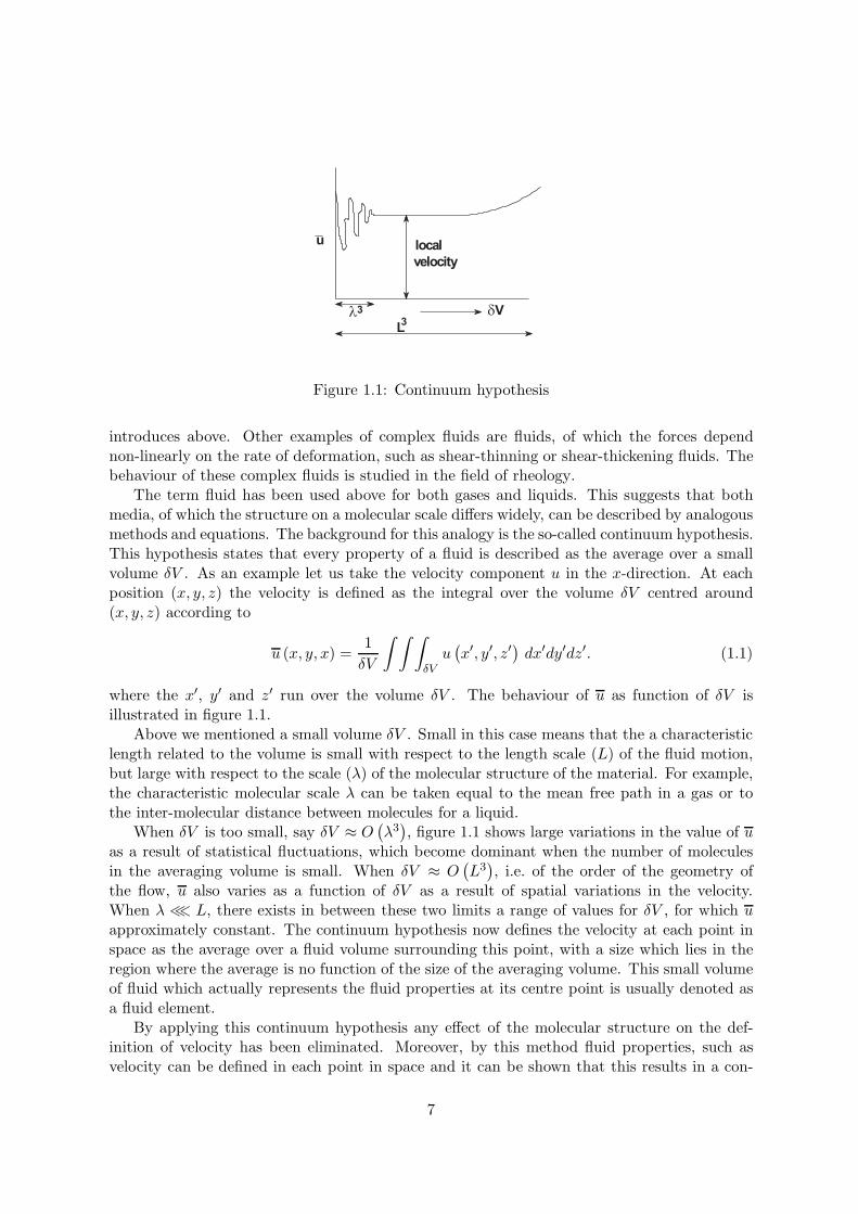
Figure 1.1: Continuum hypothesis

introduces above. Other examples of complex fluids are fluids, of which the forces dependnon-linearly on the rate of deformation, such as shear-thinning or shear-thickening fluids. Thebehaviour of these complex fluids is studied in the field of rheology.

The term fluid has been used above for both gases and liquids. This suggests that bothmedia, of which the structure on a molecular scale differs widely, can be described by analogousmethods and equations. The background for this analogy is the so-called continuum hypothesis.This hypothesis states that every property of a fluid is described as the average over a smallvolume δV . As an example let us take the velocity component u in the x-direction. At eachposition (x, y, z) the velocity is defined as the integral over the volume δV centred around(x, y, z) according to

u (x, y, x) =1δV

∫ ∫ ∫δVu(x′, y′, z′

)dx′dy′dz′. (1.1)

where the x′, y′ and z′ run over the volume δV . The behaviour of u as function of δV isillustrated in figure 1.1.

Above we mentioned a small volume δV . Small in this case means that the a characteristiclength related to the volume is small with respect to the length scale (L) of the fluid motion,but large with respect to the scale (λ) of the molecular structure of the material. For example,the characteristic molecular scale λ can be taken equal to the mean free path in a gas or tothe inter-molecular distance between molecules for a liquid.

When δV is too small, say δV ≈ O(λ3), figure 1.1 shows large variations in the value of u

as a result of statistical fluctuations, which become dominant when the number of moleculesin the averaging volume is small. When δV ≈ O

(L3), i.e. of the order of the geometry of

the flow, u also varies as a function of δV as a result of spatial variations in the velocity.When λ ≪ L, there exists in between these two limits a range of values for δV , for which uapproximately constant. The continuum hypothesis now defines the velocity at each point inspace as the average over a fluid volume surrounding this point, with a size which lies in theregion where the average is no function of the size of the averaging volume. This small volumeof fluid which actually represents the fluid properties at its centre point is usually denoted asa fluid element.

By applying this continuum hypothesis any effect of the molecular structure on the def-inition of velocity has been eliminated. Moreover, by this method fluid properties, such asvelocity can be defined in each point in space and it can be shown that this results in a con-

7

tinuous and differentiable function. Therefore, the invoking of the continuum hypothesis liesat the basis of continuum mechanics of which fluid mechanics is a subdivision.

Nevertheless, it will be clear that gases and liquids must have different properties as aresult of their different molecular structure. A gas is for instance compressible while a liquidcan be considered as almost incompressible. Compressible means here that the density ρ ofthe fluid is a function of the pressure p. Thermodynamics tells us that all materials, includinggases and liquids, are compressible and the relation between density and pressure is describedby an equation of state. As mentioned above, for liquids the change in density as a result ofa pressure increase is in practical circumstances negligible and in this case we can speak of anincompressible fluid (in section 2.1 we will learn a another definition of incompressibility interms of flow behaviour). However, we can note already here that for an incompressible fluidthe pressure can no longer be a thermodynamic variable and must be defined differently. Thiswill be discussed in section 3.2.

The molecular structure of the fluid becomes also important when exchange or transportprocesses are considered, such as exchange of heat or exchange of momentum. The latterprocess forms the background of friction. In a gas molecules are far apart and interact primarilyby means of collisions. In a liquid molecules are much closer and although they can move freelywith respect to each other, they nevertheless influence each other by means of inter-molecularforces. This difference in structure has for instance a direct influence on the magnitude of theexchange coefficients for heat and momentum. In addition this difference in structure causesalso a different behaviour a function of temperature. When the temperature increases in agas, the momentum or velocity of the molecules becomes larger. As a result, collisions becomemore frequent and energy exchange during collisions becomes larger with as effect that theexchange coefficients for heat and momentum become larger. In contrast, a larger temperaturein a fluid increases the vibrations of the molecules so that they move to a larger distance withrespect to each other. Inter-molecular forces at these larger distances become weaker with asresult that coefficients for heat and momentum exchange decrease.

Problem 1.1 The continuum hypothesis fails when we consider a flow, of which the charac-teristic length scale is of the same order of magnitude as the molecular structure. Give someexamples of such flows.

Problem 1.2 Is there a characteristic time scale, below which the continuum hypothesis isno longer valid? Estimate the order of magnitude of this time scale.

1.2 Coordinate-systems

Let us introduce the term kinematics, by which we mean the description of the velocity fieldof a flow as a function of the space and time coordinates. There are basically two methods todescribe the flow: the Eulerian and Lagrangian method.

In the case of the Lagrangian description we start with a fluid element, which we followon its way through the flow. Suppose we label this fluid element with a label a. The vectorX(t;a) then gives the position of this particular fluid element (i.e. labelled by a) as a functionof time. The X(t;a) thus traces a curve in 3D-space as function of time and this curve isgenerally called a trajectory or a fluid-element path. The velocity of the fluid element is thenby definition equal to

V =dX (t;a)

dt. (1.2)

8

We can in principle do this for every fluid element assuming that each element can bedistinguished by means of a different and unique label a. The vector a can be chosen at willbut in most cases one takes the initial position of the fluid element, i.e. the position of theelement at t = t0 or a = X(t0). If we now consider that initially, i.e. t = t0, every positionin space occupied by single fluid element then all these elements can be uniquely labelled bytheir initial position. The X(t;a) for all labels a then gives a description of the complete flowfield as a function of time and by means of (1.2) we can compute the velocity at every positionand at every time.

In this Lagrangian description the independent coordinates are the a and t. The trajectoryX(t;a) is the dependent variable. The capital letter X is used here to make the distinctionbetween the trajectory of a fluid element and the position vector in a Cartesian coordinatesystem, which is indicated by x = (x, y, z) ≡ (x1, x2, x3).

In the Eulerian description the velocity vector u = (u, v,w) ≡ (u1, u2, u3) is defined ateach position and each time in the form of a vector field: u(x, t). In this case x and t are theindependent variables and the velocity field is the dependent variable.

The relationship between the Lagrangian and Eulerian description follows from the factthat the velocity at position x and time t must be equal to the velocity of the fluid particlewhich is at this position and at this particular time. In the form of an equation this implies

dX(t;a)dt

= u(x = X, t). (1.3)

From a practical point of view the Eulerian description is the easier one to use. If weput, for instance, a measuring device at a fixed position in a flow, we measure an Eulerianvariable. The Lagrangian description has advantages mainly from a theoretical point of view.For instance the equations, which govern a fluid motion, can be very conveniently and elegantlyformulated in terms of the Lagrangian description. The Lagrangian description has also itsadvantages when we want to study the motion of individual fluid elements. An example of thislatter application is the dispersion of contaminants.

Coupled to the Eulerian description formulated in some given coordinate system x, t, wecan introduce some useful concepts. These are:

• StationaryIn this case all dependent flow variables, e.g. the velocity, are not a function of time.This means that the velocity field is given by u(x), from which time t has disappeared.In the opposite case when the velocity u depends on time, we call the flow instationaryor non-stationary.

• StreamlineA streamline is defined as the line, which is everywhere tangent to the velocity vectoru(x, t) at a given time t. Note that in an instationary flow the stream-line pattern mightvary for each time instant. Based on this definition the equation, from which a streamlinecan be computed, is given by

dx1

u1 (x1, x2, x3, t)=

dx2

u2 (x1, x2, x3, t)=

dx3

u3 (x1, x2, x3, t). (1.4)

In general a streamline is not equal to the trajectory X(t) but they are identical for astationary flow.

9

• StreamtubeThis is a virtual tube in the flow field, of which the side walls are made up out ofstreamlines. The consequence is that there is no transport through the side walls, becauseat every point the velocity if parallel to the local velocity vector, or in other wordstransport, e.g. of mass, through each cross section of the tube must be the same.

• streaklineThis is a line made up out of fluid elements, which have passed at some time through agiven fixed point. A streakline results when we release smoke or dye at a fixed point inthe flow field. For a stationary flow the streakline, streamline and trajectory are identical.

• Two dimensionalIn general a flow is three dimensional, i.e. depends on the three spatial dimensions x, yand z. When, however, the velocity field in a plane is invariant for the translation alonga line perpendicular to this plane, we call the flow two dimensional. In that case the flowis completely described when we consider the flow field in a single plane. For the casewe can describe the position in this plane by the coordinates x and y, the velocity fieldis given a u = (u, v) ≡ (u1, u2) as a function of the coordinates x = (x, y) ≡ (x1, x2) andtime t. When in a two-dimensional flow there is a velocity component in the directionperpendicular to the plane, it must be by definition constant.

Problem 1.3 Let X(t;a) be the Lagrangian description of a fluid motion with a the positionof the fluid element at t = 0. Let J denote the determinant

J =

∣∣∣∣∣∣∂X1/∂a1 ∂X1/∂a2 ∂X1/∂a3

∂X2/∂a1 ∂X2/∂a2 ∂X2/∂a3

∂X3/∂a1 ∂X3/∂a2 ∂X3/∂a3

∣∣∣∣∣∣Derive Euler’s identity

DJ

Dt= J ∇ · u

Problem 1.4 Consider a two-dimensional flow with velocity components u = −αx + βt andv = αy+γt. Compute the stream-line pattern and the x- and y-component of the trajectories.

Problem 1.5 Sketch the streamlines for the flow

u = αx, v = −αx, w = 0

where α is a positive constant.Let the concentration of some pollutant in the fluid be

c (x, y, t) = βx2ye−αt,

for y > 0, where β is a constant. Does the pollutant concentration for any particular fluidelement change with time?

Problem 1.6 Consider the instationary flow

u = u0, v = kt, w = 0,

where u0 and k are positive constants. Show that the streamlines are straight lines, and sketchthem at two different times. Also show that any fluid particle follows a parabolic path as timeproceeds.

10

1.3 Material derivative

Above we have mentioned that the Eulerian description is most commonly used in practicewhen we want to describe a fluid motion. However, we need to express Lagrangian propertiesof the flow, i.e. properties of individual fluid elements, in an Eulerian frame of reference. Forinstance we may ask ourselves what is the acceleration experienced by a fluid element expressedin a Eulerian system.

Let us first consider a function G(x, t) which is a continuously differentiable function of thecoordinates x, t. This means that all partial derivatives of G exist. Let us interpret G as theproperty of a fluid element, which is at the position X(t) = x. Examples of relevant propertiesare for instance: density, temperature or pressure. We now want to express the change ofthis property as a function of time when the fluid element moves along its trajectory. Thisis called the material derivative of G and it is expressed by the following notation: DG/Dt.The question now is: how can we compute this material derivative in an Eulerian frame ofreference? To this end we consider the total differential of G as a function of x and t

dG

dt=

∂G

∂t+dx

dt

∂G

∂x+dy

dt

∂G

∂y+dz

dt

∂G

∂z

=∂G

∂t+dxi

dt

∂G

∂xi. (1.5)

The vector (dx/dt, dy/dt, dz/dt) describes an arbitrary path through three-dimensional spaceas a function of time. We now restrict this path to the trajectory Xi(t) that the fluid elementwill take: in other words dxi/dt should be equal to the velocity ui of the fluid element atthe position xi. With help of (1.3) it then follows that the material derivative in vector andCartesian tensor notation can be written as

DG

Dt=

∂G

∂t+ (u · grad)G (1.6)

DG

Dt=

∂G

∂t+ ui

∂G

∂xi. (1.7)

In this expression ∂G/∂t is usually denoted as the local derivative or local part of the totalderivative because it describes the change of G as a function of time at a fixed position inspace (note the partial derivative). The second term on the right-hand side of (1.6) and(1.7) is usually denoted as the advective derivative or advection (or sometime also convectivederivative or convection, which because of the other meaning of convection in fluid mechanicsin relation to heat transport is somewhat confusing). This advective derivative or rather theadvective part of the total derivative gives the change of G as a function of time resulting fromthe fact that the fluid element moves in a non-homogeneous scalar field G(x, y, z).

For a property G of a fluid element which does not change along its trajectory, we find thusimmediately the equation

DG

Dt= 0. (1.8)

Any property, which satisfies (1.8) is called a material property. An example is the interfacebetween two immiscible fluids, which moves with the flow at the position of the interface andis thus a material property.

Above we have expressed the material derivative for a scalar property G. However, thematerial derivative can be also extended to a vector property. Let us take as an example the

11

flow velocity u ≡ ui. The material derivative of the velocity at position and time (x, t) can beinterpreted as the acceleration of the fluid element, which is at time t on the position x wherethe material derivative is taken. When the acceleration is calculated in a Cartesian frame ofreference then there is no problem and we can basically extend (1.7) to the velocity leadingto

Dui

Dt=∂ui

∂t+ uj

∂ui

∂xj. (1.9)

(note that repeated indices have to be summed over all coordinates, which is called the Einsteinsummation convention).

However, in a non-Cartesian (but still orthogonal) coordinate system the material derivativeof a vector becomes more complex. The background of this additional complexity is the factthat in a non-Cartesian frame of reference the direction of the unit-vectors is usually a functionof position. Let us illustrate this with help of the computation of the acceleration (i.e. thematerial derivative of the velocity) in a frame of reference, which is aligned with the localvelocity vector. In this frame of reference the unit vectors are: (es, en1, en2), where s is thecoordinate along unit vector es which is aligned with the velocity vector. The velocity vectoris then given by u(x, t) = (us(s, n1, n2), 0, 0) where n1 and n2 are the coordinates along unitvectors en1 and en2, which are perpendicular to the velocity vector. The material derivativeof u then becomes

DuDt

=∂u∂t

+ (u · grad)u

=∂u∂t

+ us∂

∂s[us(s, n1, n2) es] .

We should now note that the direction of unit vector es in principle varies as a function of thecoordinate s. In general we can write

∂es

∂s=

en

R(1.10)

where R is the radius of curvature and the unit vector en lies in the plane spanned by the unitvectors en1 and en2. With these results we find for the components of the acceleration alongthe s and n direction [

DuDt

]s

=∂us

∂t+ us

∂us

∂s(1.11)[

DuDt

]n

=u2

s

R. (1.12)

The expression in (1.11) is equivalent to the definition of material derivative as we have seenbefore. The result (1.12) is, however, quite different and it is known as a curvature termbecause it appears as result of the fact that the direction of the velocity changes.

The general theory behind these curvature terms and examples for various non-Cartesian(but still orthogonal systems) are given in the appendix B.

Problem 1.7 Consider the material derivative of a velocity field. Show that this accelerationis invariant under a so-called Galilean transformation (x, t) → (x′, t′):

x′ = x + V t

t′ = t

where V is a constant translation velocity.

12

Problem 1.8 Consider the transformation of problem 1.7 but now for an arbitrary translationvelocity V (t), which is a function of time. Show that in the transformed material derivative anadditional acceleration term appears equal to −dV/dt, which can be interpreted as a virtualforce.

13

Chapter 2

Kinematics

2.1 Conservation of mass

We continue our discussion on the properties of a vector field with as pertinent example forour case: the velocity field u(x, t). The velocity field should satisfy a number of conditionsor constraints and their formulation of is sometimes denoted by the term kinematics. One ofthese conditions is that a velocity field must obey the law of conservation of mass. The resultcan be interpret as our first equation of motion that a flow field must satisfy.

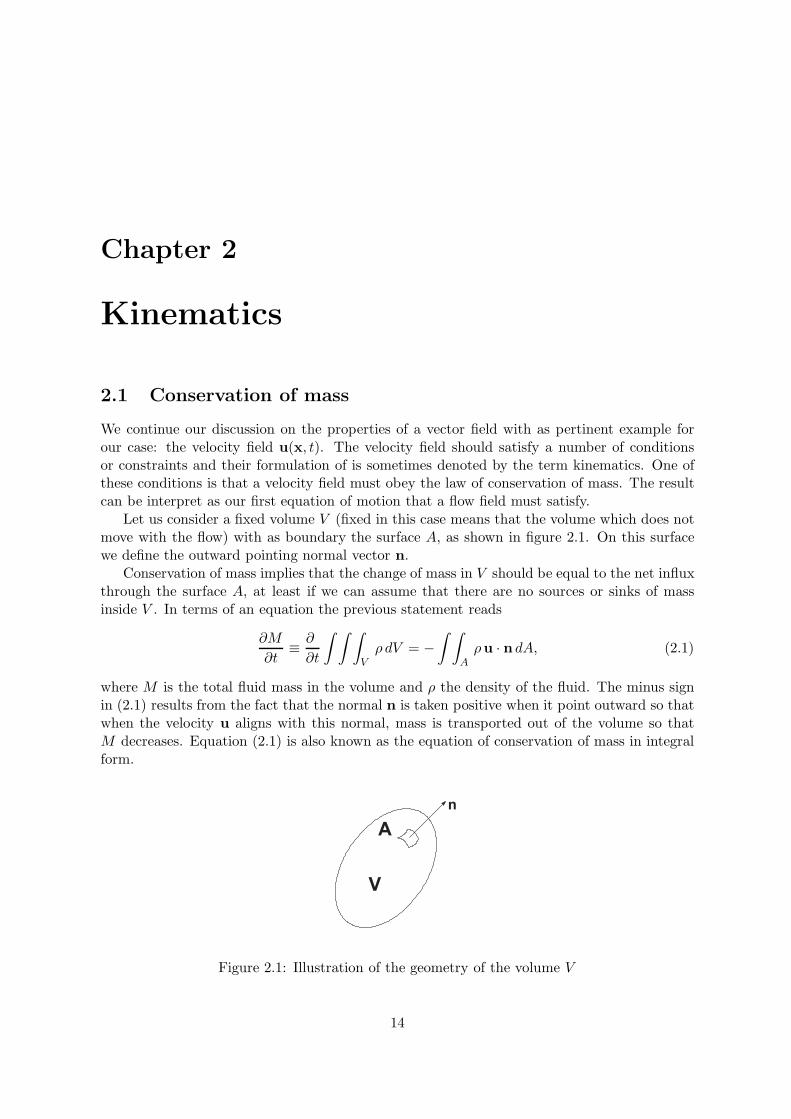
Let us consider a fixed volume V (fixed in this case means that the volume which does notmove with the flow) with as boundary the surface A, as shown in figure 2.1. On this surfacewe define the outward pointing normal vector n.

Conservation of mass implies that the change of mass in V should be equal to the net influxthrough the surface A, at least if we can assume that there are no sources or sinks of massinside V . In terms of an equation the previous statement reads

∂M

∂t≡ ∂

∂t

∫ ∫ ∫Vρ dV = −

∫ ∫Aρu · n dA, (2.1)

where M is the total fluid mass in the volume and ρ the density of the fluid. The minus signin (2.1) results from the fact that the normal n is taken positive when it point outward so thatwhen the velocity u aligns with this normal, mass is transported out of the volume so thatM decreases. Equation (2.1) is also known as the equation of conservation of mass in integralform.

V

A

n

Figure 2.1: Illustration of the geometry of the volume V

14

With help of the Gauss divergence theorem (A.9) we can transform the right-hand side of(2.1) in a volume integral. The result becomes∫ ∫ ∫

V

∂ρ

∂tdV = −

∫ ∫ ∫V

div(ρu) dV (2.2)

and because this relationship must be valid for an arbitrary volume V we can derive that

∂ρ

∂t+ div(ρu) = 0 or

Dρ

Dt+ ρ divu = 0. (2.3)

where we have used (1.6) to obtain the latter expression. This equation which is sometimesdenoted as the continuity equation, states the conservation of mass in differential form.

Based on (2.3) it is possible to give a simple interpretation of the concept of divergence.Consider a fluid element with a volume δV (remember the continuum hypothesis) and with amass δM . Conservation of mass for this fluid element reads

DδM

Dt= 0. (2.4)

To satisfy conservation of mass we must follow this fluid element on its path through the flowand for that reason we have used in the equation above the material derivative.

The mass δM can be written alternatively as δM = ρδV . After substitution in (2.4) andafter using (2.3) we can write

divu =1δV

DδV

Dt≡ ∆. (2.5)

In other words the divergence of the velocity field is the (local) relative change of volume, ∆,that a fluid element experiences in the flow field.

Next we introduce an important simplification for our equation for the mass conservation.Let us assume Dρ/Dt = 0 or the density of the fluid (inside the fluid element) does notchange during the course that the fluid element takes through the flow. Such a flow is calledincompressible and from (2.3) it follows directly that in this case the continuity equationreduces to

divu = 0. (2.6)

A velocity field that satisfies this condition is sometimes called solenoidal. The law of conser-vation of mass thus reduces in this case to a geometric condition that the velocity field shouldbe divergence free.

To arrive at (2.6) we have only assumed that the ρ of the fluid element along its trajectorythrough the flow field should remain constant. This leaves the possibility open that (at anygiven time) the ρ can still be a function of position. In other words the ρ can be different fordifferent fluid elements but for each individual element the density remains constant. A flowfor which this latter condition is satisfied, is called stratified or heterogeneous. Here we shallalways assume that besides Dρ/Dt = 0 the density also satisfies the condition ρ = f(x, y, z) orin other words fluid is homogeneous. In that case the ρ is a constant throughout the flow fieldand is also independent of time. In that case the ρ is no longer a dependent variable but rathera material constant depending on our choice for the fluid. This assumption will considerablysimplify our equations of motion for the flow.

In practice the assumption Dρ/Dt = 0 appears to be a very good approximation for bothflows of gases and liquids under the restriction that the flow speed should not become too large.

15

This implies that in that case a gas behaves as a incompressible fluid which perhaps may seemsurprising. However, we have not said yet what we mean by low flow speeds. For this we turnto the speed of sound, which is fundamental property of every material, and it describes thepropagation velocity of small density and pressure perturbations trough the material by soundwaves. From the compressible equations of motion together with the energy equation fromthermodynamics it follows that the speed of sound c is given by

c =

√(∂p

∂ρ

)S

(2.7)

where S stands for entropy. Equation (2.7) relates the speed of sound to the partial derivativeof pressure with respect to density at constant entropy. In any flow there are also pressurevariations as a result of deformations and accelerations. As we shall see later, these pressureperturbations can be estimated as δp ∝ 1/2 ρv2 where v is the flow speed. With help of (2.7),which we can write as δp ∝ c2δρ we then can find for the density perturbations

δρ v2

c2ρ

So it follows that the assumption of incompressible flow is valid when the velocity remainsmuch lower than the speed of sound, which for air is approximately ∼ 300ms−1 and for water∼ 1800ms−1.

2.2 Stream function

In a number of cases we can solve the condition (2.6) for an incompressible flow directly byintroducing a single scalar function. The first step is that we have to restrict ourselves to atwo-dimensional flow in a Cartesian frame of reference: i.e. u = (u, v) as a function of thecoordinates x = (x, y). Next we define a function ψ(x, y), which satisfies

u =∂ψ

∂y, v = −∂ψ

∂x. (2.8)

By substitution it can be shown that (2.8) satisfies (2.6) provided that ψ is at least twicedifferentiable.

The function ψ is called the stream function. and the line ψ = constant is a streamline.The latter result follows from the identity u · grad(ψ) = 0 which can be proven with help of(2.8).

The value of the stream function ψ has a specific interpretation. For this we consider twofixed points O and P in a flow field as shown in figure 2.2. The volume transport Q throughthe line segment which connects the points O and P , becomes

Q = −∫ P

Ou · n d (2.9)

where n is the normal on the line segment as indicated in figure 2.2. The minus sign is aconvention given by the condition that Q is taken positive when volume flux has a counter-clockwise direction around P . By decomposition of the integrand in (2.9) in the components

16

O

Pn

dl

uu

u

u

x

y

PO

Figure 2.2: Interpretation of the value of ψ

along the x− and y−axis and by making use of (2.8) it follows that

Q = −∫ P

O(unx + vny)d

=∫ P

O(u dy − v dx)

=∫ P

Odψ = ψ(P ) − ψ(O). (2.10)

The result appears to be independent of the particular choice of the connecting line betweenP and O.

We have thus found that the difference between the values of ψ at two positions is equal tothe volume transport through an arbitrary line which connects these positions. It follows thatthis volume transport does not change when the points P and O move along the streamlinewhich passes through their original positions. In other words the volume transport betweentwo streamlines is constant. We can make use of this result to interpret an isoline plot of thestream function ψ. Namely, except for the fact that the lines ψ = constant are streamlines andthus give the direction of the flow, it also follows that the distance between two streamlines isa measure for the magnitude of the velocity. To explain this we consider two streamlines whichlie close to each other: ψ and ψ+ dψ. The volume transport between these streamlines is thusdψ = constant ∼ |u| |d|, where |u| is the velocity of the flow in between these streamlines and|d| is the distance between the streamlines. Because anywhere along these two streamlinesdψ = constant, it follows that |d| ∼ 1/ |u| or the smaller the distance between the streamlinesthe larger the velocity.

The concept of stream function can be extended to other quasi two-dimensional geometries,such as rotation or axisymmetric flows. Let us take as an example an incompressible flow inthe cylinder coordinates x, σ, φ. Axisymmetry implies ∂/∂φ = 0. The continuity equation inthis case becomes

1σ

∂(σv)∂σ

+∂u

∂x= 0 (2.11)

where u is the velocity component along the x−axis (the axial direction) and v the componentalong the σ−axis (the radial direction) (see appendix B). The ψ(σ, x) for this geometry should

17

then satisfy

u =1σ

∂ψ

∂σ, v = − 1

σ

∂ψ

∂x(2.12)

and it is called the Stokes stream function. Its interpretation is comparable with the streamfunction for the two-dimensional Cartesian geometry, i.e. the streamlines give the direction ofthe flow and the difference between the stream function in two points gives the total volumetransport between the two streamlines passing through these points. However, the distancebetween two streamlines can not be directly taken as an estimate for the magnitude of thevelocity of the flow between the streamlines because the volume transport between two neigh-bouring streamlines dψ is in this case given by dψ 2πr |u| |d| with |d| again the distancebetween the two streamlines and r is the radial distance of the two points to the rotation axis.

Finally, for a spherical coordinate system x = (r, θ, φ) with the velocity components u =(ur, uθ, uφ) (see appendix B) it follows for the stream function, ψ(r, θ), in an axisymmetricalgeometry (i.e. ∂/∂φ = 0)

ur =1

r2 sin θ∂ψ

∂θ

uθ = − 1r sin θ

∂ψ

∂r. (2.13)

Problem 2.1 Calculate the stream function for the following 2-D flow in Cartesian coordi-nates

u = αx, v = −αx, w = 0

where α is a constant. Sketch the resulting streamline pattern.

Problem 2.2 Calculate the stream function for the following axisymmetric flow in sphericalcoordinates

ur = −32U

(1 − r2

a2

)cos θ, uθ =

32U

(1 − 2

r2

a2

)sin θ, uφ = 0

where U and a are constants and r ≤ a. Sketch the resulting streamline pattern

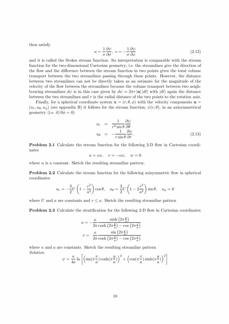
Problem 2.3 Calculate the stratification for the following 2-D flow in Cartesian coordinates

u = − κ

2asinh

(2π y

a

)cosh

(2π y

a

)− cos(2π x

a

)v =

κ

2asin(2π x

a

)cosh

(2π y

a

)− cos(2π x

a

)where κ and a are constants. Sketch the resulting streamline patternSolution

ψ =κ

4aln[(

sin(πx

a) cosh(π

y

a))2

+(cos(π

x

a) sinh(π

y

a))2]

18

•

•

x

x+ xx

uu+ u

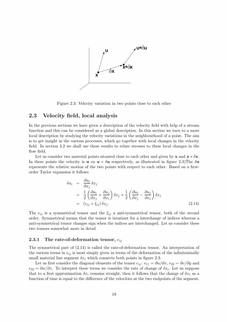
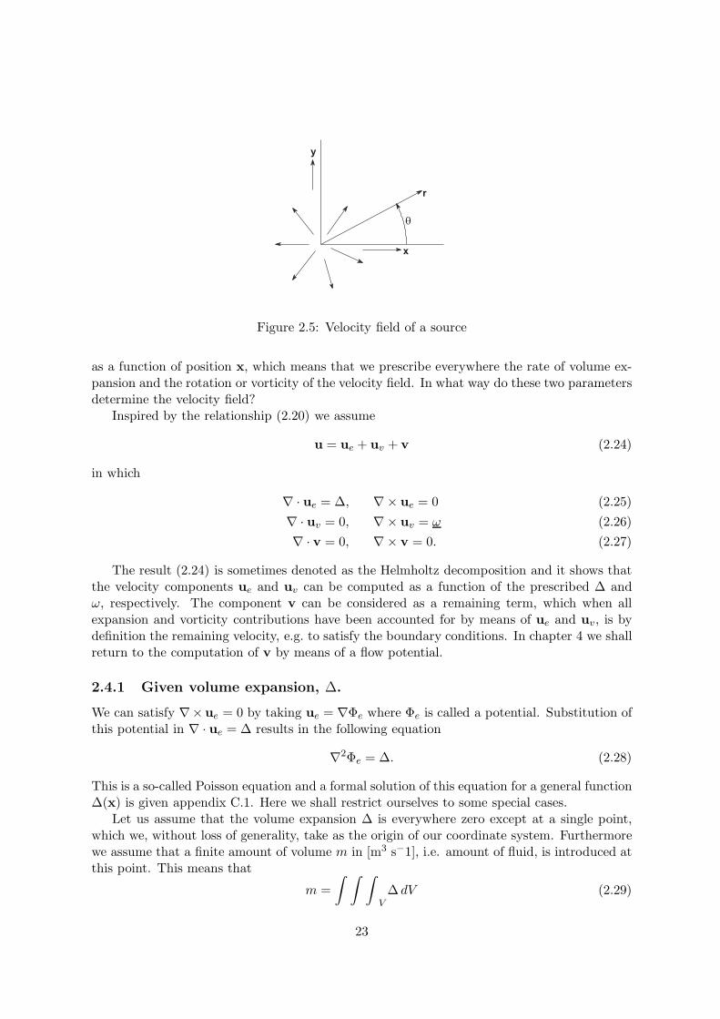
Figure 2.3: Velocity variation in two points close to each other

2.3 Velocity field, local analysis

In the previous sections we have given a description of the velocity field with help of a streamfunction and this can be considered as a global description. In this section we turn to a morelocal description by studying the velocity variations in the neighbourhood of a point. The aimis to get insight in the various processes, which go together with local changes in the velocityfield. In section 3.2 we shall use these results to relate stresses to these local changes in theflow field.

Let us consider two material points situated close to each other and given by x and x+ δx.In these points the velocity is u en u + δu respectively, as illustrated in figure 2.3)The δurepresents the relative motion of the two points with respect to each other. Based on a first-order Taylor expansion it follows

δui =∂ui

∂xjδxj

=12

(∂ui

∂xj+∂uj

∂xi

)δxj +

12

(∂ui

∂xj− ∂uj

∂xi

)δxj

= (eij + ξij) δxj . (2.14)

The eij is a symmetrical tensor and the ξij a anti-symmetrical tensor, both of the secondorder. Symmetrical means that the tensor is invariant for a interchange of indices whereas aanti-symmetrical tensor changes sign when the indices are interchanged. Let us consider thesetwo tensors somewhat more in detail

2.3.1 The rate-of-deformation tensor, eij

The symmetrical part of (2.14) is called the rate-of-deformation tensor. An interpretation ofthe various terms in eij is most simply given in terms of the deformation of the infinitesimallysmall material line segment δxi which connects both points in figure 2.3.

Let us first consider the diagonal elements of the tensor eij : e11 = ∂u/∂x, e22 = ∂v/∂y ande33 = ∂w/∂z. To interpret these terms we consider the rate of change of δxi. Let us supposethat to a first approximation δxi remains straight, then it follows that the change of δxi as afunction of time is equal to the difference of the velocities at the two endpoints of the segment.

19

x

y

v

1

2 x dx

uy dy

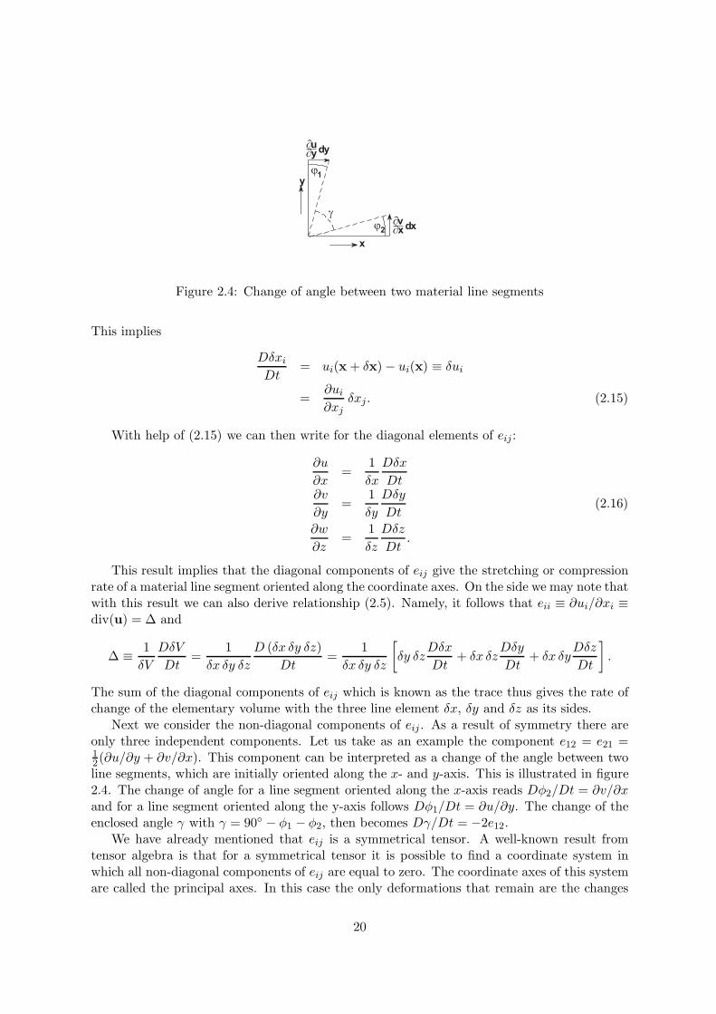
Figure 2.4: Change of angle between two material line segments

This implies

Dδxi

Dt= ui(x + δx) − ui(x) ≡ δui

=∂ui

∂xjδxj . (2.15)

With help of (2.15) we can then write for the diagonal elements of eij :

∂u

∂x=

1δx

Dδx

Dt∂v

∂y=

1δy

Dδy

Dt(2.16)

∂w

∂z=

1δz

Dδz

Dt.

This result implies that the diagonal components of eij give the stretching or compressionrate of a material line segment oriented along the coordinate axes. On the side we may note thatwith this result we can also derive relationship (2.5). Namely, it follows that eii ≡ ∂ui/∂xi ≡div(u) = ∆ and

∆ ≡ 1δV

DδV

Dt=

1δx δy δz

D (δx δy δz)Dt

=1

δx δy δz

[δy δz

Dδx

Dt+ δx δz

Dδy

Dt+ δx δy

Dδz

Dt

].

The sum of the diagonal components of eij which is known as the trace thus gives the rate ofchange of the elementary volume with the three line element δx, δy and δz as its sides.

Next we consider the non-diagonal components of eij . As a result of symmetry there areonly three independent components. Let us take as an example the component e12 = e21 =12(∂u/∂y + ∂v/∂x). This component can be interpreted as a change of the angle between twoline segments, which are initially oriented along the x- and y-axis. This is illustrated in figure2.4. The change of angle for a line segment oriented along the x-axis reads Dφ2/Dt = ∂v/∂xand for a line segment oriented along the y-axis follows Dφ1/Dt = ∂u/∂y. The change of theenclosed angle γ with γ = 90 − φ1 − φ2, then becomes Dγ/Dt = −2e12.

We have already mentioned that eij is a symmetrical tensor. A well-known result fromtensor algebra is that for a symmetrical tensor it is possible to find a coordinate system inwhich all non-diagonal components of eij are equal to zero. The coordinate axes of this systemare called the principal axes. In this case the only deformations that remain are the changes

20

in length by either stretching or compression of the line segments along the coordinate axes.These are called the principal components.

In short we can interpret the tensor eij in terms of a change of the length of a line segmenteither by stretching or compression when the line segment is oriented in the direction of oneof the principal axes. For another direction along (non-principal) coordinate axis we have acombination of change of length and change of direction of the line segment.

2.3.2 The rotation tensor, ξij

The anti-symmetric tensor ξij is also known as the rotation tensor for reasons which willbecome clear below. An anti-symmetric tensor has at most three independent non-diagonalcomponents not equal to zero (the diagonal component are zero by definition). It is thereforepossible to express these components with help of a vector ωk. Let us pose

ξij = −12εijk ωk, (2.17)

in which εijk is the permutation tensor which satisfies the condition of anti-symmetry, i.e. theinterchange of any two of the three indices of εijk results in a change of sign.

The anti-symmetric part of δui according to (2.14) can then be written as follows

δuai = −1

2εijk δxj ωk

=12εijk ωj δxk

=12ω × δx. (2.18)

This result implies that δuai can be interpreted as a solid body rotation of the two points in

figure 2.3 with respect to each other. In other words 12ω gives the local rotation of a fluid

element, i.e. the direction of ω gives the rotation axis and half the length of ω the angularvelocity.

The question now arises: what it the relationship between ω and the velocity field? To thisend we compute the expression εmji ξij. Making use of the equation (A.5) it follows that

ωk = εkji∂ui

∂xj≡ ∇× u (2.19)

or ω is equal to the rotation of the velocity field defined according to (A.8). With this resultwe have thus found an interpretation for the rotation of a vector field in terms of twice thelocal rotation of an element. The variable ωk defined according to (2.19) will be frequentlyencountered in the following under the name vorticity.

2.3.3 Local description of the velocity field

Let us now return to the beginning of this section, namely to equation (2.14). Based on theresults derived above it follows that we can write the velocity field in the neighbourhood of apoint x as the sum of three contributions given by

ui(x + δx) = ui(x) + eij δxj +12εijk ωj δxk. (2.20)

21

The first term on the right-hand side of (2.20) can be interpreted as a pure translation. Aswe have seen in 2.3.1, the second term represents the rate of deformation of a fluid element interms of changes in length of the sides of the element and in terms of changes in shape as aresult of a change in angle between two line element. The third term on the right-hand sideof (2.20) can be interpreted as solid body rotation with an angular velocity equal to half theabsolute value of the rotational operator applied to the velocity field.

The contribution due to deformation can be subdivided further according to

eij δxj = 13∆ δij + (eij − 1

3∆ δij) δxj (2.21)

The first term on the right-hand side can be interpreted as an isotropic change of volume. Thismeans a change in size of the fluid element which is equal in all directions (note that as a resultof Einstein’s summation convention δii = 3). The second term represents a deviation from thisisotropic change of volume and can therefore be interpreted as a pure change in shape of thefluid element with a conservation of volume.

Problem 2.4 Given is a 3 ∗ 3 tensor tij . Show with help of the characteristic equation forthe eigenvalues that there are three invariants of tij, where invariant means that these valuesremain constant under a coordinate transformation, which is rotation over an arbitrary angle.Are these all the invariants?

Problem 2.5 On a rectangular sheet of rubber we draw a rectangle with its sides parallel tothe sides of the rubber sheet. How does the rectangle appear when

1. one pulls at the sheet with equal strength at two opposites sides;

2. one pulls at all four sides of the sheet with for the opposite sides with equal strength butwith unequal strength for adjoining sides.

3. one pulls at the four corners of the sheet with equal strength

Problem 2.6 Compute the deformation and rotation tensor for the velocity fields given inproblems 1.4, 1.5 and 1.6. Indicate the areas of stretching and compression and where there isrotation.

Problem 2.7 Separate the shear flow u = (βy, 0, 0) into its local translation, rotation anddeformation contributions. What are in this case the principal axes?

2.4 Velocity field, global analysis

We have seen that by a local analysis the velocity field in the neighbourhood of a point can bedecomposed into a component, eij , describing the rate of deformation and a component, ξij ,which the gives the local rotation. Let us now turn this result around and ask ourselves thequestion: if we prescribe the rate-of deformation and the local rotation, can we then reconstructthe velocity field?

Let us simplify this problem somewhat. Suppose that we give

∆ = divu (2.22)ω = rotu (2.23)

22

x

y

r

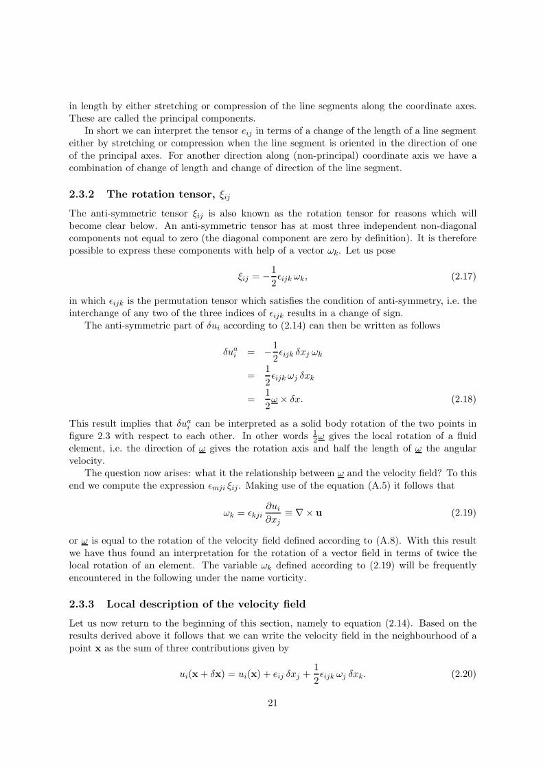
Figure 2.5: Velocity field of a source

as a function of position x, which means that we prescribe everywhere the rate of volume ex-pansion and the rotation or vorticity of the velocity field. In what way do these two parametersdetermine the velocity field?

Inspired by the relationship (2.20) we assume

u = ue + uv + v (2.24)

in which

∇ · ue = ∆, ∇× ue = 0 (2.25)∇ · uv = 0, ∇× uv = ω (2.26)∇ · v = 0, ∇× v = 0. (2.27)

The result (2.24) is sometimes denoted as the Helmholtz decomposition and it shows thatthe velocity components ue and uv can be computed as a function of the prescribed ∆ andω, respectively. The component v can be considered as a remaining term, which when allexpansion and vorticity contributions have been accounted for by means of ue and uv, is bydefinition the remaining velocity, e.g. to satisfy the boundary conditions. In chapter 4 we shallreturn to the computation of v by means of a flow potential.

2.4.1 Given volume expansion, ∆.

We can satisfy ∇×ue = 0 by taking ue = ∇Φe where Φe is called a potential. Substitution ofthis potential in ∇ · ue = ∆ results in the following equation

∇2Φe = ∆. (2.28)

This is a so-called Poisson equation and a formal solution of this equation for a general function∆(x) is given appendix C.1. Here we shall restrict ourselves to some special cases.

Let us assume that the volume expansion ∆ is everywhere zero except at a single point,which we, without loss of generality, take as the origin of our coordinate system. Furthermorewe assume that a finite amount of volume m in [m3 s−1], i.e. amount of fluid, is introduced atthis point. This means that

m =∫ ∫ ∫

V∆ dV (2.29)

23

O

sink source

x

-m m

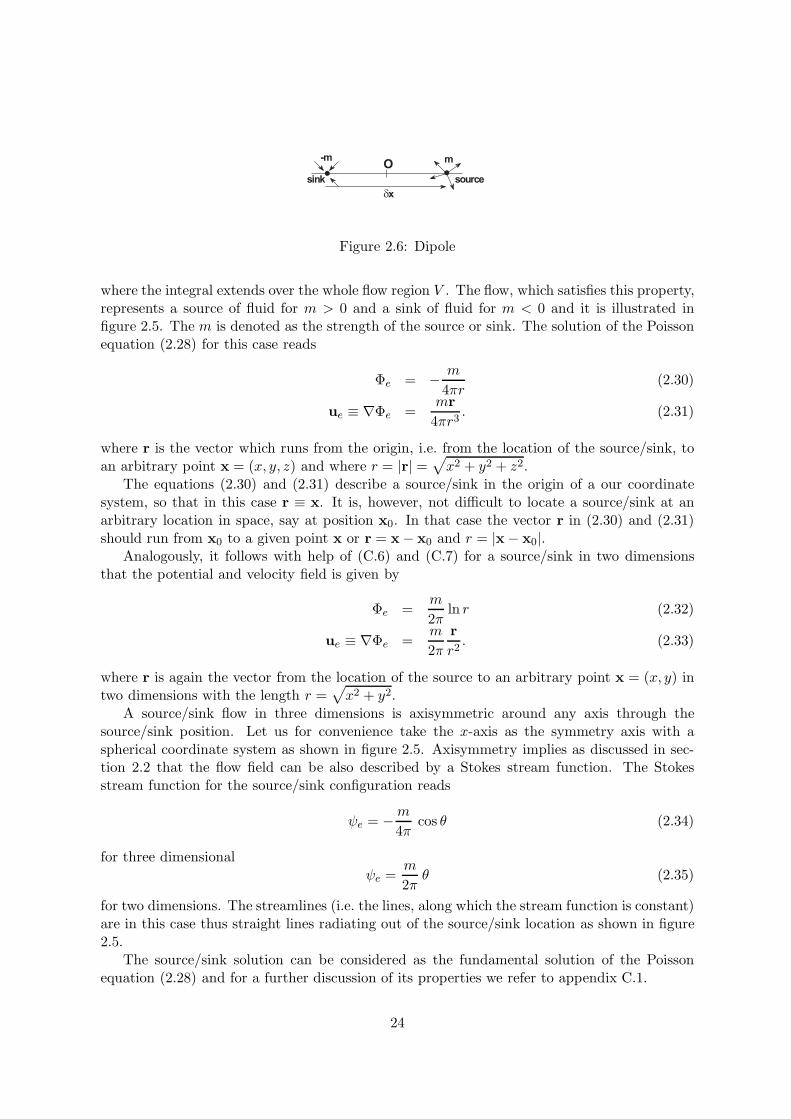
Figure 2.6: Dipole

where the integral extends over the whole flow region V . The flow, which satisfies this property,represents a source of fluid for m > 0 and a sink of fluid for m < 0 and it is illustrated infigure 2.5. The m is denoted as the strength of the source or sink. The solution of the Poissonequation (2.28) for this case reads

Φe = − m

4πr(2.30)

ue ≡ ∇Φe =mr

4πr3. (2.31)

where r is the vector which runs from the origin, i.e. from the location of the source/sink, toan arbitrary point x = (x, y, z) and where r = |r| =

√x2 + y2 + z2.

The equations (2.30) and (2.31) describe a source/sink in the origin of a our coordinatesystem, so that in this case r ≡ x. It is, however, not difficult to locate a source/sink at anarbitrary location in space, say at position x0. In that case the vector r in (2.30) and (2.31)should run from x0 to a given point x or r = x− x0 and r = |x− x0|.

Analogously, it follows with help of (C.6) and (C.7) for a source/sink in two dimensionsthat the potential and velocity field is given by

Φe =m

2πln r (2.32)

ue ≡ ∇Φe =m

2πrr2. (2.33)

where r is again the vector from the location of the source to an arbitrary point x = (x, y) intwo dimensions with the length r =

√x2 + y2.

A source/sink flow in three dimensions is axisymmetric around any axis through thesource/sink position. Let us for convenience take the x-axis as the symmetry axis with aspherical coordinate system as shown in figure 2.5. Axisymmetry implies as discussed in sec-tion 2.2 that the flow field can be also described by a Stokes stream function. The Stokesstream function for the source/sink configuration reads

ψe = −m

4πcos θ (2.34)

for three dimensionalψe =

m

2πθ (2.35)

for two dimensions. The streamlines (i.e. the lines, along which the stream function is constant)are in this case thus straight lines radiating out of the source/sink location as shown in figure2.5.

The source/sink solution can be considered as the fundamental solution of the Poissonequation (2.28) and for a further discussion of its properties we refer to appendix C.1.

24

The Poisson is a linear differential equation and this type of differential equation has theproperty that the sum of two solutions is again a solution. This is called the superpositionprinciple. Let us use this principle to construct a solution which consists of a source withstrength m (m > 0) on the x-axis at a distance 0.5δx from the origin and a sink with strength−m on the x-axis with a distance −0.5δx from the origin (see figure 2.6). This choice for equalstrengths for both the source and sink implies that the total volume expansion of this flow isequal to zero.

Let us next consider the limit for δx→ 0 with as condition

limδx→0

mδx = µ (2.36)

where µ is defined as the dipole vector with in this particular case the vector aligned along thex-axis. However, in principal the source and sink can have a general orientation with respectto the coordinate system. In that case the µ is defined as the vector (with length µ) whichpoints from the source towards the sink.

Let us return to the case where the dipole is oriented along the x-axis. With help of (2.30)and (2.32) and by taking the limit δx → 0 subject to condition (2.36) we find for the case ofthree dimensions

Φe =µ

4π∂

∂x

(1r

). (2.37)

For a general orientation of the dipole vector the result becomes

Φe =µ

4π· ∇(

1r) (2.38)

Next we consider the combination of a source and sink with equal strength in two dimensionsand take the limit for the distance between the source and sink approach zero. With a conditionequivalent to (2.36) we then find

Φe = − µ

2π· ∇(ln r) (2.39)

The flows resulting from (2.38) and (2.39) are known as a dipole flow.Let us now restrict ourselves to the case where the dipole vector is oriented along the x-axis

and where the dipole itself is located in the origin of the coordinate system. The equations(2.38) and (2.39) for three and two dimensions, respectively reduce then to

Φe = − µx

4πr3(2.40)

andΦe = − µx

2πr2. (2.41)

For an arbitrary location, say x0, of the dipole we should substitute again r = |x− x0| into(2.38) and (2.39).

Like source and sink flows, dipole flows are axisymmetric around the x-axis (or in generalaround the axis along the dipole vector). So again stream functions can be introduced. Theseread

ψ =µ sin2 θ

4πr(2.42)

25

for three dimensions andψ =

µ sin θ2πr

(2.43)

for two dimensions where θ is defined as shown in figure 2.5.

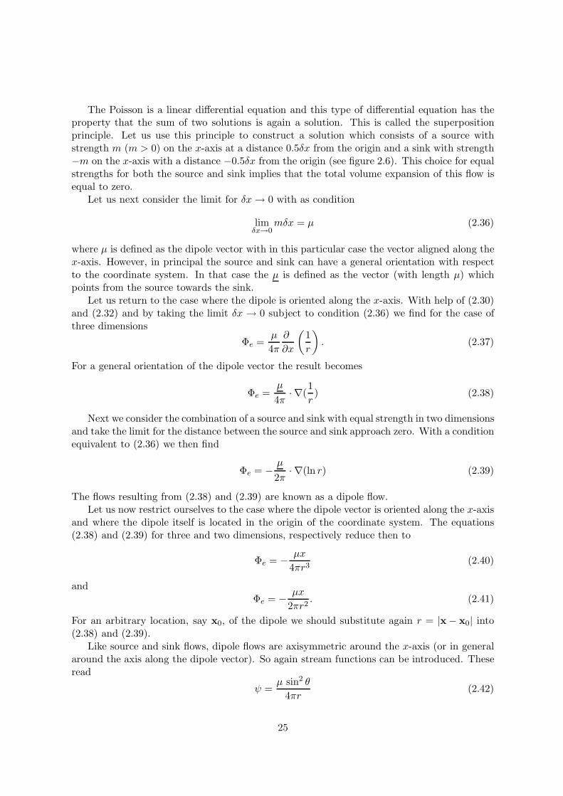
Problem 2.8 Consider a source and a sink with equal strength m and positioned on the x-axisat the locations 0.5δ and −0.5δ, respectively. Calculate and sketch the streamline patterns ofthis flow for various values of δ.

Problem 2.9 Consider a source/sink in the origin of a coordinate system with a strengthequal to 2m and two sources/sinks, each with a strength of −m, i.e. with a opposite sign withrespect to the source/sink in the origin. The two sources/sinks are positioned along the x-axisat x = δx and x = −δx, respectively. Consider the limit for δx→ 0 under the condition that

limδx→0

δx2 m = µ2

with µ2 finite. Consider this problem in two and three dimensions and sketch the resultingstreamline patterns. Is there a closed streamline, which does not pass through the origin.

Problem 2.10 Consider in two dimensions two sources with strength m each, positioned alongthe x-axis at x = 0.5 δx and x = −0.5 δx, respectively. In addition consider two sinks withstrength −m each, positioned along the y-axis at y = 0.5 δy and y = −0.5 δy, respectively.Consider the limit for δx→ 0 and δy → 0 under the condition that

limδx→0

limδy→0

δxδy m = µ12

with µ12 finite. Sketch the resulting streamline patterns. This flow is known as a quadrupole

Problem 2.11 Extend problem 2.10 to three dimensions. In that case we have two sourceswith strength m each, positioned along the x-axis at x = 0.5 δx and x = −0.5 δx, respectivelyand two sources positioned along the z-axis at z = 0.5 δz and z = −0.5 δz, respectively. Inaddition consider two sinks with strength −2m each, positioned along the z-axis at z = 0.5 δzand z = −0.5 δz, respectively. Consider the limit for δx → 0, δy → 0 and δz → 0 under thecondition that

limδx→0

limδy→0

limδz→0

δxδyδz m = µ123

with µ123 finite. Sketch the resulting streamline patterns.

Problem 2.12 Consider a homogenous surface distribution of sources on a disk with radiusR and with a total integrated source strength equal to M . Determine the direction of thevelocity on the symmetry axis and compute the potential on this symmetry axis. Based onthis potential discuss and sketch the magnitude of the velocity along the symmetry axis as afunction of the distance to the disk

26

A

A

n

n

1

1

1

2

2

2

Figure 2.7: Vortex line and vortex tube

2.4.2 Given vorticity distribution, ωi

Let us go back to the equations (2.26). We can satisfy ∇·uv = 0 by taking ue = ∇×Bv whereBv is called a vector potential. In appendix C.2 we show how we can compute with help ofthis vector potential the velocity field uv for the case of a general vorticity distribution ω asfunction of the space coordinates. Here we shall restrict ourselves again to some special cases.

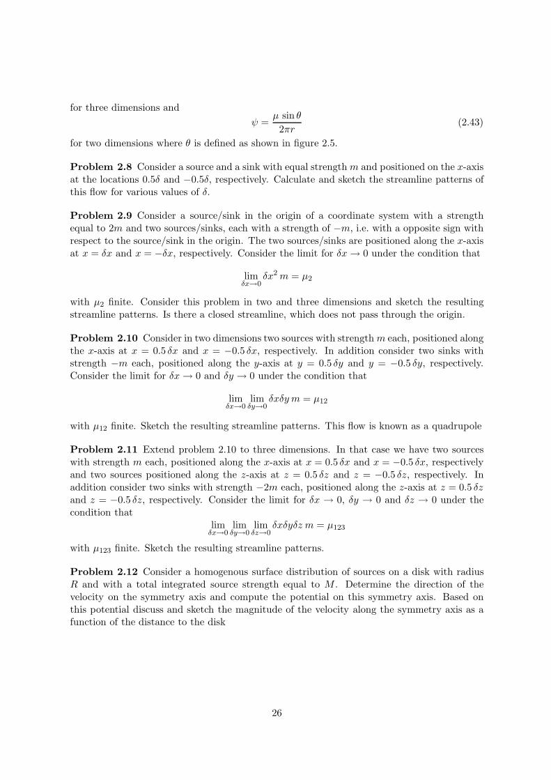
In analogy with the flow field for a given volume expansion treated in the previous sectionone would perhaps expect that the fundamental solution is again a point source, in this case apoint source of vorticity. However, this is not the case. The reason for this lies in a propertyof the vorticity defined as the rotation of the velocity field. Namely, a general property oftwo vector fields a (x) and b (x) with a = ∇ × b ≡ rotb is that ∇ · a ≡ div a = 0. A pointsource can never satisfy this latter criterion because at the position of the point source thedivergence is always unequal to zero. The alternative is to concentrate the vorticity not in apoint but in a line and in appendix C.2 we show that there exists a solution for this case whichis denoted a line vortex. Before we consider the consequences of this solution, we turn first tosome definitions and general properties of vorticity distributions.

First we introduce the notion vortex line, which is defined as the line which is at everyposition tangent to the vorticity vector ω as shown in figure 2.7. Returning to our discussionon a streamline given in section 1.2 we thus see that a vortex line is comparable to a streamline.Next we define a vortex tube as a tube of which the side wall are made up by vortex lines asillustrated in figure 2.7 (note the similarity to the definition of a stream tube). The strengthof a vortex tube is defined as

κ =∫ ∫

Aω · n dA (2.44)

where A is an arbitrary cross-section of the tube and n is the normal op vector on A withits direction chosen parallel to the direction of the ω in the wall of the vortex tube. Theintersection of A with the vortex tube gives rise to the closed curve Γ.

It can now be proved that the strength κ stays constant for every cross section along thevortex tube. This follows from applying the condition (A.15), according to which the divergenceof the rotation is equal to zero, in the divergence theorem (A.9). For the integration volumewe choose a volume enclosed by two cross-sections A1 en A2 (see figure 2.7) and the wall of

27

x

y

z

s

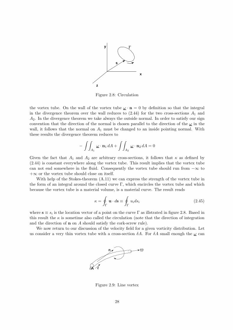
Γ

Figure 2.8: Circulation

the vortex tube. On the wall of the vortex tube ω · n = 0 by definition so that the integralin the divergence theorem over the wall reduces to (2.44) for the two cross-sections A1 andA2. In the divergence theorem we take always the outside normal. In order to satisfy our signconvention that the direction of the normal is chosen parallel to the direction of the ω in thewall, it follows that the normal on A1 must be changed to an inside pointing normal. Withthese results the divergence theorem reduces to

−∫ ∫

A1

ω · n1 dA+∫ ∫

A2

ω · n2 dA = 0

Given the fact that A1 and A2 are arbitrary cross-sections, it follows that κ as defined by(2.44) is constant everywhere along the vortex tube. This result implies that the vortex tubecan not end somewhere in the fluid. Consequently the vortex tube should run from −∞ to+∞ or the vortex tube should close on itself.

With help of the Stokes-theorem (A.11) we can express the strength of the vortex tube inthe form of an integral around the closed curve Γ, which encircles the vortex tube and whichbecause the vortex tube is a material volume, is a material curve. The result reads

κ =∮

Γu · ds ≡

∮Γuidsi (2.45)

where s ≡ si is the location vector of a point on the curve Γ as illstrated in figure 2.8. Based inthis result the κ is sometime also called the circulation (note that the direction of integrationand the direction of n on A should satisfy the cork-screw rule).

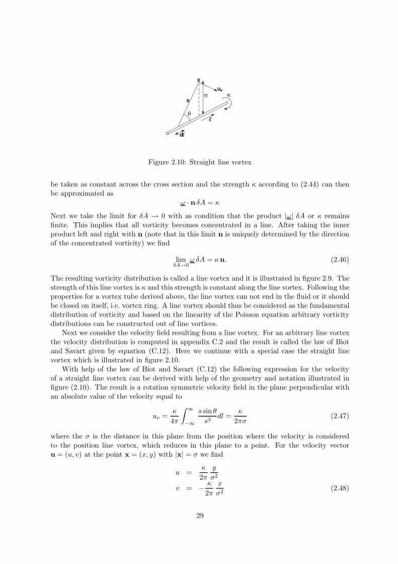
We now return to our discussion of the velocity field for a given vorticity distribution. Letus consider a very thin vortex tube with a cross-section δA. For δA small enough the ω can

n

A l

Figure 2.9: Line vortex

28

x

s

uv

dl

l

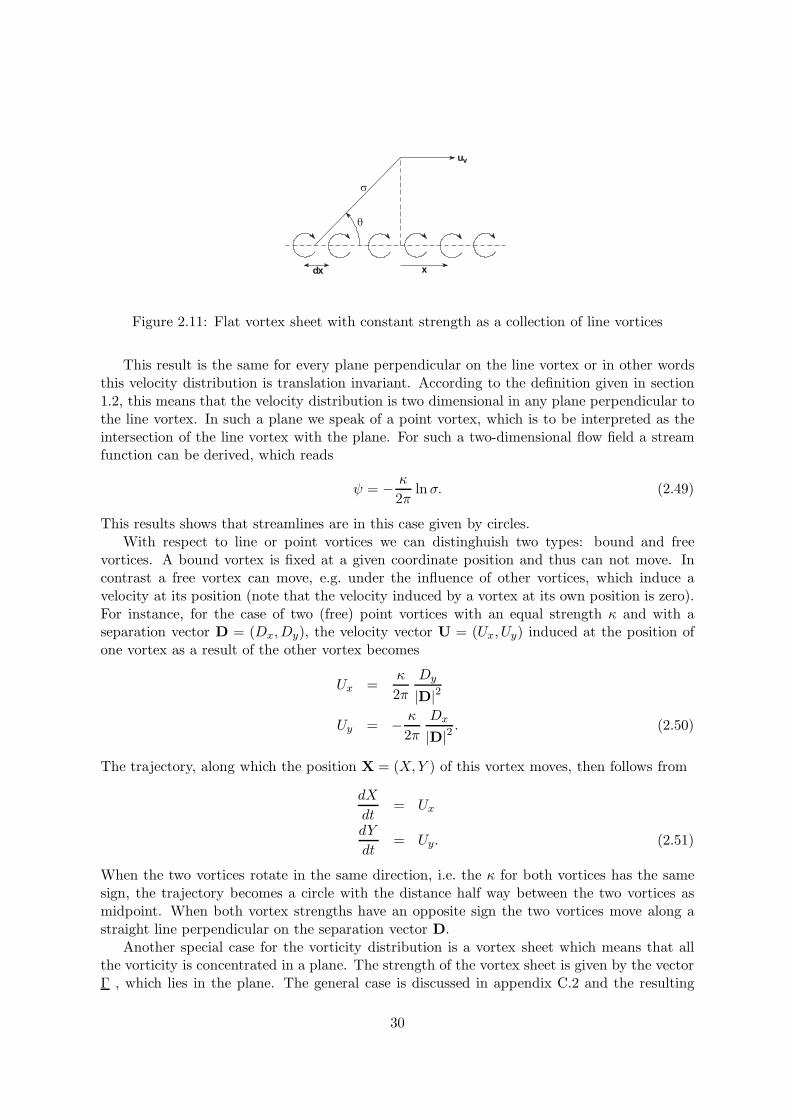
Figure 2.10: Straight line vortex

be taken as constant across the cross section and the strength κ according to (2.44) can thenbe approximated as

ω · n δA = κ

Next we take the limit for δA → 0 with as condition that the product |ω| δA or κ remainsfinite. This implies that all vorticity becomes concentrated in a line. After taking the innerproduct left and right with n (note that in this limit n is uniquely determined by the directionof the concentrated vorticity) we find

limδA→0

ω δA = κn. (2.46)

The resulting vorticity distribution is called a line vortex and it is illustrated in figure 2.9. Thestrength of this line vortex is κ and this strength is constant along the line vortex. Following theproperties for a vortex tube derived above, the line vortex can not end in the fluid or it shouldbe closed on itself, i.e. vortex ring. A line vortex should thus be considered as the fundamentaldistribution of vorticity and based on the linearity of the Poisson equation arbitrary vorticitydistributions can be constructed out of line vortices.

Next we consider the velocity field resulting from a line vortex. For an arbitrary line vortexthe velocity distribution is computed in appendix C.2 and the result is called the law of Biotand Savart given by equation (C.12). Here we continue with a special case the straight linevortex which is illustrated in figure 2.10.

With help of the law of Biot and Savart (C.12) the following expression for the velocityof a straight line vortex can be derived with help of the geometry and notation illustrated infigure (2.10). The result is a rotation symmetric velocity field in the plane perpendicular withan absolute value of the velocity equal to

uv =κ

4π

∫ ∞

−∞

s sin θs3

dl =κ

2πσ(2.47)

where the σ is the distance in this plane from the position where the velocity is consideredto the position line vortex, which reduces in this plane to a point. For the velocity vectoru = (u, v) at the point x = (x, y) with |x| = σ we find

u =κ

2πy

σ2

v = − κ

2πx

σ2(2.48)

29

xdx

uv

Figure 2.11: Flat vortex sheet with constant strength as a collection of line vortices

This result is the same for every plane perpendicular on the line vortex or in other wordsthis velocity distribution is translation invariant. According to the definition given in section1.2, this means that the velocity distribution is two dimensional in any plane perpendicular tothe line vortex. In such a plane we speak of a point vortex, which is to be interpreted as theintersection of the line vortex with the plane. For such a two-dimensional flow field a streamfunction can be derived, which reads

ψ = − κ

2πlnσ. (2.49)

This results shows that streamlines are in this case given by circles.With respect to line or point vortices we can distinghuish two types: bound and free

vortices. A bound vortex is fixed at a given coordinate position and thus can not move. Incontrast a free vortex can move, e.g. under the influence of other vortices, which induce avelocity at its position (note that the velocity induced by a vortex at its own position is zero).For instance, for the case of two (free) point vortices with an equal strength κ and with aseparation vector D = (Dx,Dy), the velocity vector U = (Ux, Uy) induced at the position ofone vortex as a result of the other vortex becomes

Ux =κ

2πDy

|D|2

Uy = − κ

2πDx

|D|2 . (2.50)

The trajectory, along which the position X = (X,Y ) of this vortex moves, then follows from

dX

dt= Ux

dY

dt= Uy. (2.51)

When the two vortices rotate in the same direction, i.e. the κ for both vortices has the samesign, the trajectory becomes a circle with the distance half way between the two vortices asmidpoint. When both vortex strengths have an opposite sign the two vortices move along astraight line perpendicular on the separation vector D.

Another special case for the vorticity distribution is a vortex sheet which means that allthe vorticity is concentrated in a plane. The strength of the vortex sheet is given by the vectorΓ , which lies in the plane. The general case is discussed in appendix C.2 and the resulting

30

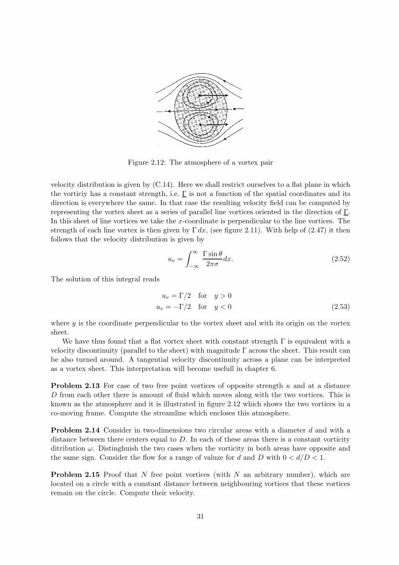
Figure 2.12: The atmosphere of a vortex pair

velocity distribution is given by (C.14). Here we shall restrict ourselves to a flat plane in whichthe vorticiy has a constant strength, i.e. Γ is not a function of the spatial coordinates and itsdirection is everywhere the same. In that case the resulting velocity field can be computed byrepresenting the vortex sheet as a series of parallel line vortices oriented in the direction of Γ.In this sheet of line vortices we take the x-coordinate is perpendicular to the line vortices. Thestrength of each line vortex is then given by Γ dx, (see figure 2.11). With help of (2.47) it thenfollows that the velocity distribution is given by

uv =∫ ∞

−∞

Γ sin θ2πσ

dx. (2.52)

The solution of this integral reads

uv = Γ/2 for y > 0uv = −Γ/2 for y < 0 (2.53)

where y is the coordinate perpendicular to the vortex sheet and with its origin on the vortexsheet.

We have thus found that a flat vortex sheet with constant strength Γ is equivalent with avelocity discontinuity (parallel to the sheet) with magnitude Γ across the sheet. This result canbe also turned around. A tangential velocity discontinuity across a plane can be interpretedas a vortex sheet. This interpretation will become usefull in chapter 6.

Problem 2.13 For case of two free point vortices of opposite strength κ and at a distanceD from each other there is amount of fluid which moves along with the two vortices. This isknown as the atmosphere and it is illustrated in figure 2.12 which shows the two vortices in aco-moving frame. Compute the streamline which encloses this atmosphere.

Problem 2.14 Consider in two-dimensions two circular areas with a diameter d and with adistance between there centers equal to D. In each of these areas there is a constant vorticityditribution ω. Distinghuish the two cases when the vorticity in both areas have opposite andthe same sign. Consider the flow for a range of valuze for d and D with 0 < d/D < 1.

Problem 2.15 Proof that N free point vortices (with N an arbitrary number), which arelocated on a circle with a constant distance between neighbouring vortices that these vorticesremain on the circle. Compute their velocity.

31

Problem 2.16 Consider a pair of two free point vortices with opposite strengths κ and initiallyat a distance D from each other. The pair approaches an infinite wall which is oriented parallelto the separation vector. Compute the trajectory of both vortices for the case of an ideal, non-viscous fluid. What happens for the case of an real viscous fluid. Consider also the case whenthe wall make an angle with the separation vector and the is finite

y

x

b

a

r

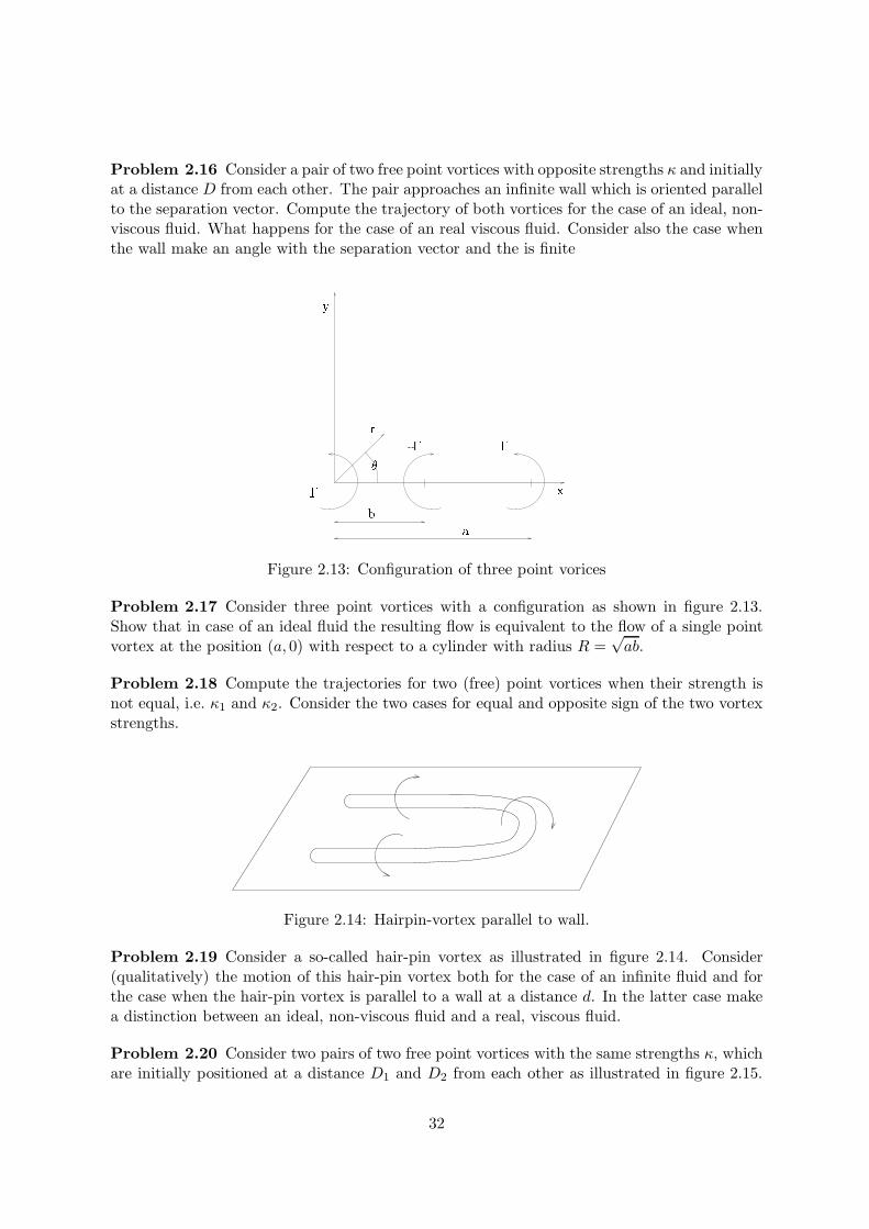
Figure 2.13: Configuration of three point vorices

Problem 2.17 Consider three point vortices with a configuration as shown in figure 2.13.Show that in case of an ideal fluid the resulting flow is equivalent to the flow of a single pointvortex at the position (a, 0) with respect to a cylinder with radius R =

√ab.

Problem 2.18 Compute the trajectories for two (free) point vortices when their strength isnot equal, i.e. κ1 and κ2. Consider the two cases for equal and opposite sign of the two vortexstrengths.

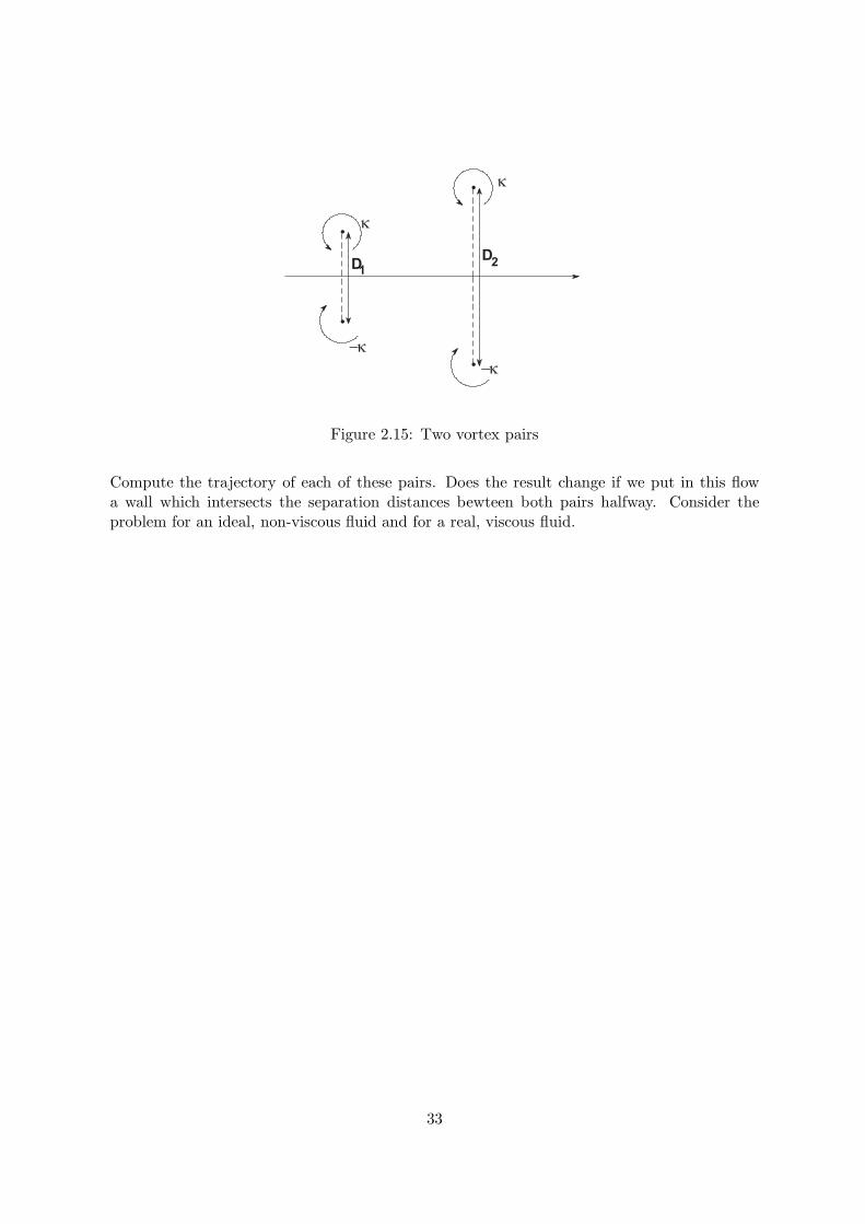
Figure 2.14: Hairpin-vortex parallel to wall.

Problem 2.19 Consider a so-called hair-pin vortex as illustrated in figure 2.14. Consider(qualitatively) the motion of this hair-pin vortex both for the case of an infinite fluid and forthe case when the hair-pin vortex is parallel to a wall at a distance d. In the latter case makea distinction between an ideal, non-viscous fluid and a real, viscous fluid.

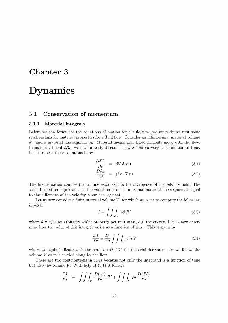
Problem 2.20 Consider two pairs of two free point vortices with the same strengths κ, whichare initially positioned at a distance D1 and D2 from each other as illustrated in figure 2.15.

32

•

•

•

•

DD

12

Figure 2.15: Two vortex pairs

Compute the trajectory of each of these pairs. Does the result change if we put in this flowa wall which intersects the separation distances bewteen both pairs halfway. Consider theproblem for an ideal, non-viscous fluid and for a real, viscous fluid.

33

Chapter 3

Dynamics

3.1 Conservation of momentum

3.1.1 Material integrals

Before we can formulate the equations of motion for a fluid flow, we must derive first somerelationships for material properties for a fluid flow. Consider an infinitesimal material volumeδV and a material line segment δx. Material means that these elements move with the flow.In section 2.1 and 2.3.1 we have already discussed how δV en δx vary as a function of time.Let us repeat these equations here:

DδV

Dt= δV divu (3.1)

DδxDt

= (δx · ∇)u. (3.2)

The first equation couples the volume expansion to the divergence of the velocity field. Thesecond equation expresses that the variation of an infinitesimal material line segment is equalto the difference of the velocity along the segment.

Let us now consider a finite material volume V , for which we want to compute the followingintegral

I =∫ ∫ ∫

Vρθ dV (3.3)

where θ(x, t) is an arbitrary scalar property per unit mass, e.g. the energy. Let us now deter-mine how the value of this integral varies as a function of time. This is given by

DI

Dt≡ D

Dt

∫ ∫ ∫Vρθ dV (3.4)

where we again indicate with the notation D /Dt the material derivative, i.e. we follow thevolume V as it is carried along by the flow.

There are two contributions in (3.4) because not only the integrand is a function of timebut also the volume V . With help of (3.1) it follows

DI

Dt=

∫ ∫ ∫V

D(ρθ)Dt

dV +∫ ∫ ∫

VρθD(dV )Dt

34

=∫ ∫ ∫

VρDθ

DtdV +

∫ ∫ ∫Vθ

(Dρ

Dt+ ρdivu

)dV

=∫ ∫ ∫

VρDθ

DtdV (3.5)

where we have used (2.3) to obtain the last expression.For the extension to integrals along material lines and material surfaces we refer to section

3.1 of Batchelor.

3.1.2 Conservation of momentum in differential form

The term dynamics implies the study of fluid motion as a consequence of the equations ofmotion of Newton expressed in terms of conservation of momentum. Point of departure is amaterial volume V . The velocity u ≡ ui can be interpreted as the momentum per unit massand the combination ρui where ρ is the density, can be interpreted as the momentum per unitvolume. Conservation of momentum for the volume V according to Newton’s second law thenreads

D

Dt

∫ ∫ ∫Vρui dV = Fi (3.6)

where Fi is the resultant of all forces that work on V .The forces Fi can be subdivided into two types: volume and surface forces:

F = Fvol + Fsurf . (3.7)

Let us turn first to the volume forces Fvol. A general characterisation of a volume force can begiven as a force, which is effective over a large distance. The influence of this force can thusbe felt everywhere in the volume V . For that reason a volume force is sometime also called abody force. Examples of volume forces are: the force of gravity, electrical forces or the virtualforce, e.g. due to the acceleration of the frame of reference, which we shall consider furtherin section 3.3.3. Due to their large range of influence these forces will vary only slowly as afunction of distance. From this it follows that their effect on an infinitesimal volume elementdV is proportional to the volume. This leads to

dFvol = ρf dV (3.8)

where f is a parameter with the dimension of acceleration. In the following we shall makemost frequently use of f = g where g = (0, 0,−g) is the acceleration of gravity in a coordinatesystem for which the positive z-axis is taken vertically upwards (i.e. the g points along thenegative z-axis). Another example is the flow in a coordinate system, which accelerates withf0 with respect to an inertial coordinate system. In that case the flow experiences a volumeforce with f equal to f = −f0.

Based on (3.8) it follows that the total or resultant volume force on V becomes equal to

Fvol =∫ ∫ ∫

Vρf dV, (3.9)

which for f = g is equal tot the weight of the fluid mass in volume V .Next we consider the surface forces Fsurf . These forces are effective only over a very small

distance which is of the order of the separation distance between individual molecules. The

35

Σn

dS

1

2

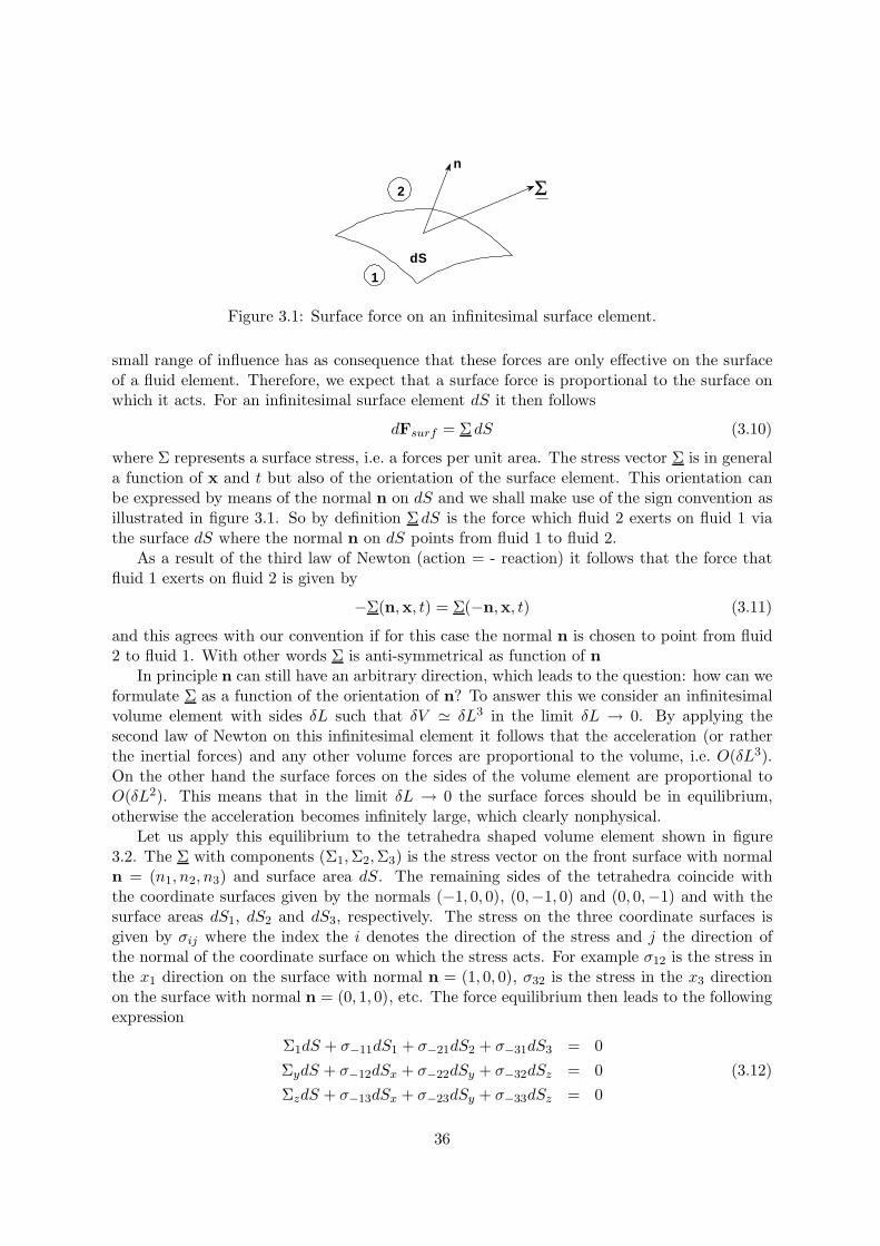
Figure 3.1: Surface force on an infinitesimal surface element.

small range of influence has as consequence that these forces are only effective on the surfaceof a fluid element. Therefore, we expect that a surface force is proportional to the surface onwhich it acts. For an infinitesimal surface element dS it then follows

dFsurf = Σ dS (3.10)

where Σ represents a surface stress, i.e. a forces per unit area. The stress vector Σ is in generala function of x and t but also of the orientation of the surface element. This orientation canbe expressed by means of the normal n on dS and we shall make use of the sign convention asillustrated in figure 3.1. So by definition Σ dS is the force which fluid 2 exerts on fluid 1 viathe surface dS where the normal n on dS points from fluid 1 to fluid 2.

As a result of the third law of Newton (action = - reaction) it follows that the force thatfluid 1 exerts on fluid 2 is given by

−Σ(n,x, t) = Σ(−n,x, t) (3.11)

and this agrees with our convention if for this case the normal n is chosen to point from fluid2 to fluid 1. With other words Σ is anti-symmetrical as function of n

In principle n can still have an arbitrary direction, which leads to the question: how can weformulate Σ as a function of the orientation of n? To answer this we consider an infinitesimalvolume element with sides δL such that δV δL3 in the limit δL → 0. By applying thesecond law of Newton on this infinitesimal element it follows that the acceleration (or ratherthe inertial forces) and any other volume forces are proportional to the volume, i.e. O(δL3).On the other hand the surface forces on the sides of the volume element are proportional toO(δL2). This means that in the limit δL → 0 the surface forces should be in equilibrium,otherwise the acceleration becomes infinitely large, which clearly nonphysical.

Let us apply this equilibrium to the tetrahedra shaped volume element shown in figure3.2. The Σ with components (Σ1,Σ2,Σ3) is the stress vector on the front surface with normaln = (n1, n2, n3) and surface area dS. The remaining sides of the tetrahedra coincide withthe coordinate surfaces given by the normals (−1, 0, 0), (0,−1, 0) and (0, 0,−1) and with thesurface areas dS1, dS2 and dS3, respectively. The stress on the three coordinate surfaces isgiven by σij where the index the i denotes the direction of the stress and j the direction ofthe normal of the coordinate surface on which the stress acts. For example σ12 is the stress inthe x1 direction on the surface with normal n = (1, 0, 0), σ32 is the stress in the x3 directionon the surface with normal n = (0, 1, 0), etc. The force equilibrium then leads to the followingexpression

Σ1dS + σ−11dS1 + σ−21dS2 + σ−31dS3 = 0ΣydS + σ−12dSx + σ−22dSy + σ−32dSz = 0 (3.12)ΣzdS + σ−13dSx + σ−23dSy + σ−33dSz = 0

36

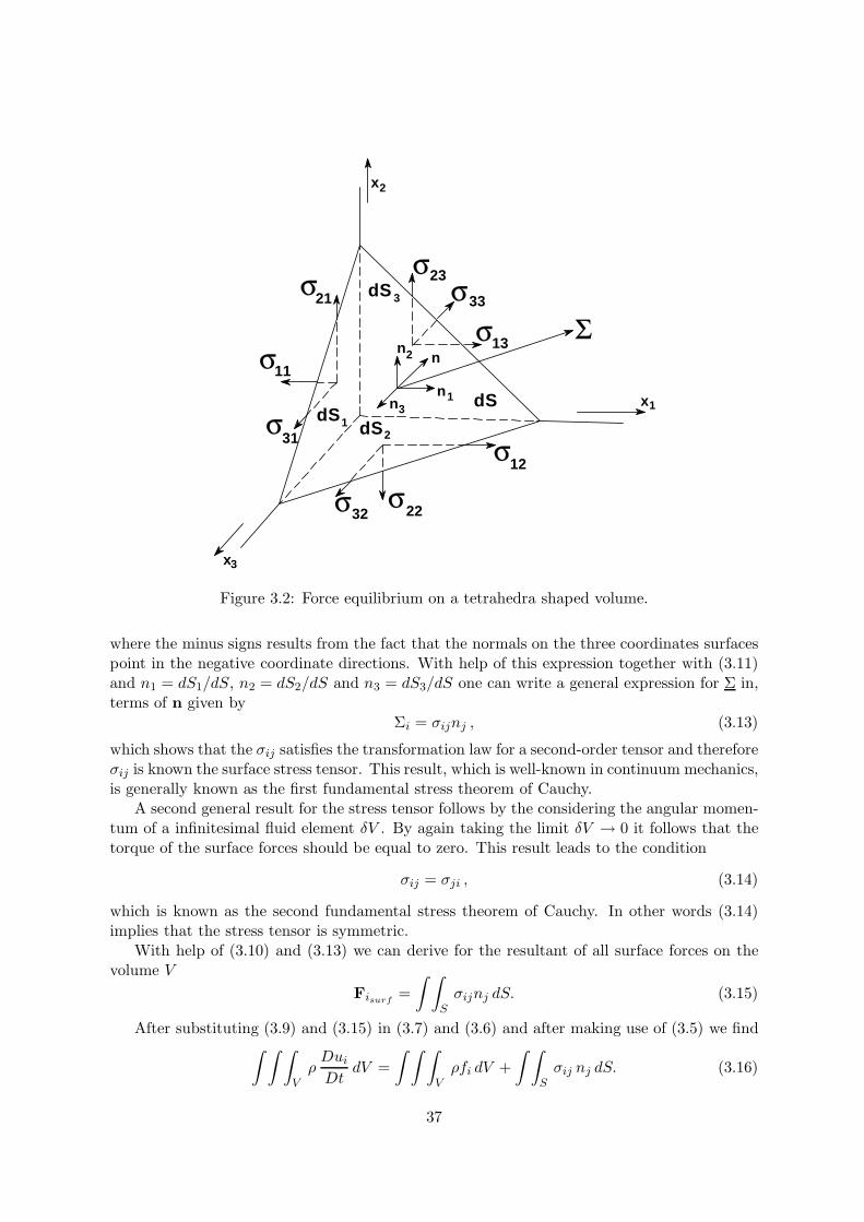
Σσ

σ

σ

σσ

σ

σσ

σ11

12

13

21

22

23

31

32

33

x

x

x

1

2

3

n

n

n

n 1

2

3 dSdS

dS

dS

12

3

Figure 3.2: Force equilibrium on a tetrahedra shaped volume.

where the minus signs results from the fact that the normals on the three coordinates surfacespoint in the negative coordinate directions. With help of this expression together with (3.11)and n1 = dS1/dS, n2 = dS2/dS and n3 = dS3/dS one can write a general expression for Σ in,terms of n given by

Σi = σijnj , (3.13)

which shows that the σij satisfies the transformation law for a second-order tensor and thereforeσij is known the surface stress tensor. This result, which is well-known in continuum mechanics,is generally known as the first fundamental stress theorem of Cauchy.

A second general result for the stress tensor follows by the considering the angular momen-tum of a infinitesimal fluid element δV . By again taking the limit δV → 0 it follows that thetorque of the surface forces should be equal to zero. This result leads to the condition

σij = σji , (3.14)

which is known as the second fundamental stress theorem of Cauchy. In other words (3.14)implies that the stress tensor is symmetric.

With help of (3.10) and (3.13) we can derive for the resultant of all surface forces on thevolume V

Fisurf=∫ ∫

Sσijnj dS. (3.15)

After substituting (3.9) and (3.15) in (3.7) and (3.6) and after making use of (3.5) we find∫ ∫ ∫VρDui

DtdV =

∫ ∫ ∫Vρfi dV +

∫ ∫Sσij nj dS. (3.16)

37

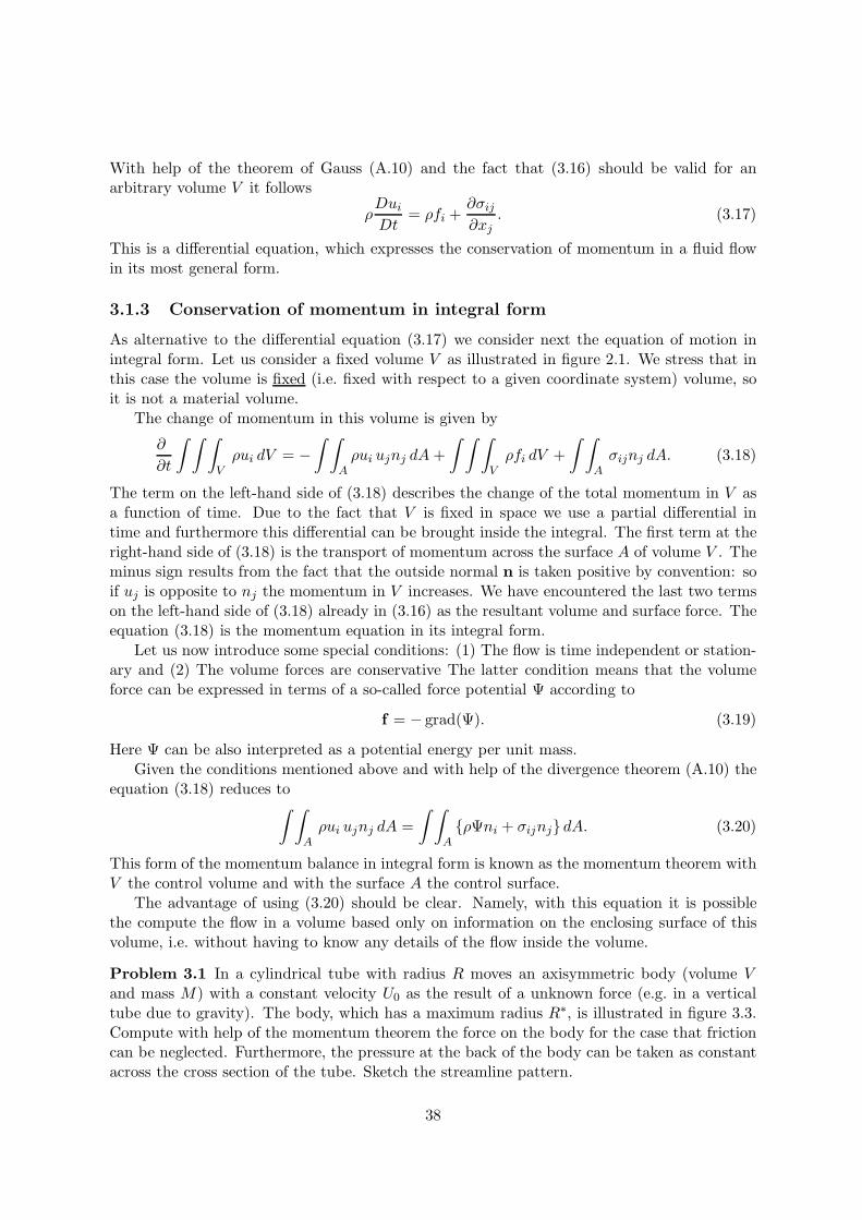
With help of the theorem of Gauss (A.10) and the fact that (3.16) should be valid for anarbitrary volume V it follows

ρDui

Dt= ρfi +

∂σij

∂xj. (3.17)

This is a differential equation, which expresses the conservation of momentum in a fluid flowin its most general form.

3.1.3 Conservation of momentum in integral form

As alternative to the differential equation (3.17) we consider next the equation of motion inintegral form. Let us consider a fixed volume V as illustrated in figure 2.1. We stress that inthis case the volume is fixed (i.e. fixed with respect to a given coordinate system) volume, soit is not a material volume.

The change of momentum in this volume is given by

∂

∂t

∫ ∫ ∫Vρui dV = −

∫ ∫Aρui ujnj dA+

∫ ∫ ∫Vρfi dV +

∫ ∫Aσijnj dA. (3.18)

The term on the left-hand side of (3.18) describes the change of the total momentum in V asa function of time. Due to the fact that V is fixed in space we use a partial differential intime and furthermore this differential can be brought inside the integral. The first term at theright-hand side of (3.18) is the transport of momentum across the surface A of volume V . Theminus sign results from the fact that the outside normal n is taken positive by convention: soif uj is opposite to nj the momentum in V increases. We have encountered the last two termson the left-hand side of (3.18) already in (3.16) as the resultant volume and surface force. Theequation (3.18) is the momentum equation in its integral form.

Let us now introduce some special conditions: (1) The flow is time independent or station-ary and (2) The volume forces are conservative The latter condition means that the volumeforce can be expressed in terms of a so-called force potential Ψ according to

f = − grad(Ψ). (3.19)

Here Ψ can be also interpreted as a potential energy per unit mass.Given the conditions mentioned above and with help of the divergence theorem (A.10) the

equation (3.18) reduces to∫ ∫Aρui ujnj dA =

∫ ∫AρΨni + σijnj dA. (3.20)

This form of the momentum balance in integral form is known as the momentum theorem withV the control volume and with the surface A the control surface.

The advantage of using (3.20) should be clear. Namely, with this equation it is possiblethe compute the flow in a volume based only on information on the enclosing surface of thisvolume, i.e. without having to know any details of the flow inside the volume.

Problem 3.1 In a cylindrical tube with radius R moves an axisymmetric body (volume Vand mass M) with a constant velocity U0 as the result of a unknown force (e.g. in a verticaltube due to gravity). The body, which has a maximum radius R∗, is illustrated in figure 3.3.Compute with help of the momentum theorem the force on the body for the case that frictioncan be neglected. Furthermore, the pressure at the back of the body can be taken as constantacross the cross section of the tube. Sketch the streamline pattern.

38

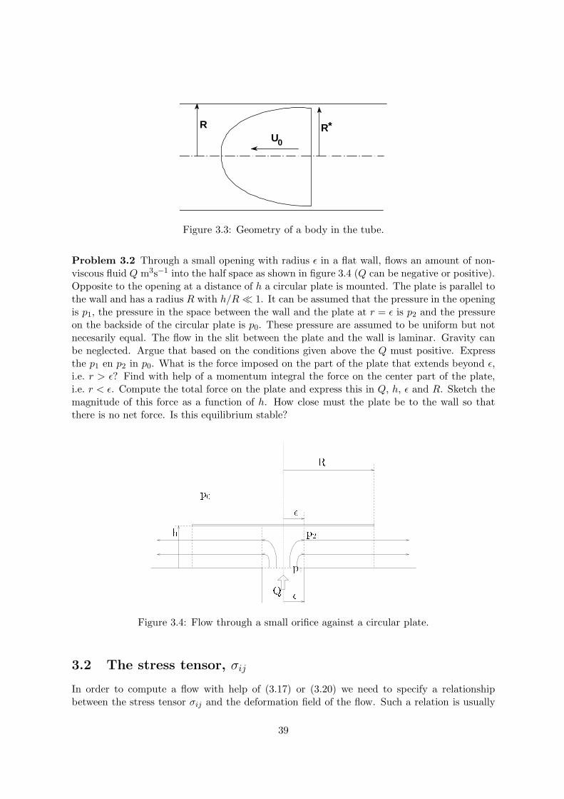
RRU

*

0

Figure 3.3: Geometry of a body in the tube.

Problem 3.2 Through a small opening with radius ε in a flat wall, flows an amount of non-viscous fluid Q m3s−1 into the half space as shown in figure 3.4 (Q can be negative or positive).Opposite to the opening at a distance of h a circular plate is mounted. The plate is parallel tothe wall and has a radius R with h/R 1. It can be assumed that the pressure in the openingis p1, the pressure in the space between the wall and the plate at r = ε is p2 and the pressureon the backside of the circular plate is p0. These pressure are assumed to be uniform but notnecesarily equal. The flow in the slit between the plate and the wall is laminar. Gravity canbe neglected. Argue that based on the conditions given above the Q must positive. Expressthe p1 en p2 in p0. What is the force imposed on the part of the plate that extends beyond ε,i.e. r > ε? Find with help of a momentum integral the force on the center part of the plate,i.e. r < ε. Compute the total force on the plate and express this in Q, h, ε and R. Sketch themagnitude of this force as a function of h. How close must the plate be to the wall so thatthere is no net force. Is this equilibrium stable?

p

R

h

Q

p

p

Figure 3.4: Flow through a small orifice against a circular plate.

3.2 The stress tensor, σij

In order to compute a flow with help of (3.17) or (3.20) we need to specify a relationshipbetween the stress tensor σij and the deformation field of the flow. Such a relation is usually

39

denoted as a constitutive relationship.Let us first consider the stress tensor in somewhat more detail. We have already mentioned

that σijnj is the component of the stress in the i-direction, which acts on a surface with anoutside normal nj. What do the individual component of σij mean? First, we take one of thediagonal components, i.e. i = j. In that case the stress acts in the same direction as the normalon the surface and for that reason we call this a normal stress. If in this case the direction of thestress σ is parallel to n we call it a tension stress and a compression stress when the directionof the stress is opposite to the normal. Second, we consider the non-diagonal components, i.e.i =/ j. In this case the stress is perpendicular to n or the stress lies in the plane of the surfacethat is considered. In this case one speaks of a shear stress. In general a shear stress has twocomponents.

As a result of (3.14) it follows that σij is a symmetric tensor. Similarly as we have seenfor the rate of deformation tensor eij in section 2.3.1, it is then possible to find a coordinatesystem in which only the diagonal terms of σij are nonzero. Such a coordinate system is calleda principal coordinate system and the stresses in this system, which are only normal stresses,are the principal stresses. In other words in a principal coordinate system we find only tensionor compression stresses.

For any tensor we can define a number of invariants. These are parameters that areindependent of the coordinate system, in which the tensor is expressed and which are thusinvariant under a coordinate transformation. One of these invariants is the trace, which isequal to the sum of the diagonal elements. For the stress tensor σij the trace becomes: σ11 +σ22 + σ33 ≡ σii or the trace is the sum of the normal stresses. From this it follows that 1

3σii

can be interpreted as the mean normal stress. Based on this result we can write for the stresstensor

σij =13σkk δij + (σij − 1

3σkk δij) =

13σkk δij + dij . (3.21)

The first term on the right-hand side of (3.21) can then be interpreted as a isotropic normalstress, i.e. a normal stress which is the same in all coordinate directions. The second term canthen be considered as the deviation of the isotropic normal stress and for that reason it is alsodenoted as the deviatoric stress dij .

The main question that we have to answer is: what is the connection between the stressesaccording to (3.21) and the deformation, which is described in terms of the rate of deformationtensor eij defined in (2.14) and discussed in section 2.3.1. It seems obvious that the isotropicnormal stress (note that by definition shear stresses can not be isotropic) has to connect torate of change of volume, while the deviatoric stress will rather cause a change of shape.Given this background we will now determine a relationship between the stress and the rateof deformation.

3.2.1 Stress in a fluid at rest

Let us first consider a fluid in rest, i.e. without any motion with respect to a given coordinatesystem or in other words each fluid element remains at the same position and does not changeits shape. From our definition of a fluid discussed in section ?? it follows that in this casethe deviatoric stress must be identical equal to zero because we have argued above that thedeviatoric stresses change the shape of fluid elements. In other words the stresses in a fluid inrest are given by

σij =13σkk δij = −p δij. (3.22)

40

In this case we thus find that the only stress in the fluid is an isotropic normal stress whichwe call the pressure p.. The pressure is defined to be positive when it is oriented opposite tothe normal n on a surface and this explains the minus sign in (3.22).

When we substitute (3.22) and ui = 0 in the general equation of motion (3.17) we find

0 = ρfi − ∂p

∂xi. (3.23)

This equation, which we can interpret as a balance between volume and pressure forces, de-scribes the stress condition in fluid at rest. When the force is conservative, (3.19) gives theforce in terms of a potential Ψ. For the gravitational acceleration at the earth’s surface itfollows that

Ψ = g z, (3.24)

where z is the height above the surface. This expression can be interpreted as the potentialenergy (per unit mass) in the earth’s gravitational field at a height z. For this case it thenfollows that fi = (0, 0,−g) ≡ g, which when substituted in (3.23) leads to

∂p

∂x= 0,

∂p

∂y= 0,

∂p

∂z= −ρg. (3.25)

This equation is known as the law of Pascal and it describes for instance the decrease ofpressure with height in our atmosphere. In general it gives pressure variation as function ofheight in any fluid at rest under the influence of gravity and the resulting pressure is called thehydrostatic pressure. In physical terms the law of Pascal states that the pressure at a certainlevel z is determined by the weight of the fluid above that level.

Another result that follows from (3.23) is the well-known law of Archimedes. Let us considera body with volume V and surface A which is immersed in a fluid at rest. The pressure on thesurface of the body leads to a resultant force given by

Fr = −∫ ∫

Apini dA (3.26)

where n is the outward normal to the surface. With help of the divergence theorem of Gauss(A.10) we can write

Fr = −∫ ∫ ∫

Vgrad p dV, (3.27)

which with help of (3.25) can be rewritten as

Fr = −gρV. (3.28)

This represents an upward force equal to the weight of the displaced fluid. This effect is alsodenoted as buoyancy.

Problem 3.3 For a self-gravitating fluid, such as a star in our universe, the gravitationalpotential is given by equation

∇2Ψ = 4πGρ

where G is the constant of gravitation. The relation between Ψ and p follows from (3.19) and(3.23). Derive from these equations for a spherically symmetric body the equation

d

dr

(r2

ρ

dp

dr

)= −4πGρ.

41

Solve this equation for two cases: 1. ρ = ρ0, which is constant, and 2. p = Cρ6/5 under thecondition that p→ 0 for r → ∞.

Problem 3.4 The pressure as a function of height in the corona of the sun above the solarsurface is given by the following variant of the law of Pascal (3.25)

dp

dr= −GM

r2ρ

where r is the radius to the center of the sun, G the constant of gravitation and M the massof the sun. Assume that the corona consists of an ideal gas. The temperature as a function ofheight is given by

T = T0

(r0r

) 27

where r0 is the radius of the sun and T0 the temperature on the surface of the sun. Solve theresulting equations and show that the pressure for r → ∞ does not approach zero. Interpretthis result this result in terms of the solar wind.

3.2.2 Stress in a fluid in motion

Next we turn to a fluid in motion. In that case we expect changes in the shape of fluid elementsand as a result the deviatoric stress will be not equal to zero. Nevertheless in this case wealso introduce an isotropic pressure defined as the averaged of the normal forces in the threecoordinate directions, i.e.

p = −13σii. (3.29)

This equation can be considered as the definition of the pressure in a fluid flow. The pressuredefined in this way has in principle no relationship with the so-called thermodynamic pressure,which follows from the equation of state of the medium. To distinguish the pressure accordingto (3.29) from the thermodynamic pressure it is sometimes denoted as the mechanical pressure.In chapter 5 we shall get back to the relation between the thermodynamic and the mechanicalpressure. The pressure which we have introduced here is sometimes also called the staticpressure.

For the stress tensor in a fluid flow now follows

σij = −pδij + dij. (3.30)

The next step is to express the deviatoric stress dij in terms of the deformations. We expectthat this stress can not depend on the velocity itself because that would violate Galileaninvariance. Therefore we expect a relationship between dij and the velocity gradients whichhave interpreted in 2.3. We now propose as an hypothesis that dij depends only linearly onthe velocity gradients ∂uk/∂xl according to

dij = Aijkl∂uk

∂xl. (3.31)

Here Aijkl represents a fourth-order tensor, which depends only on the fluid properties and thusno longer on the flow field. Based on our treatment of the local velocity variations discussedin section 2.3 we can write

dij = Aijkl ekl +Aijkl ξkl

= Aijkl ekl − 12Aijkl εklm ωm. (3.32)

42

With help of some hypotheses regarding the fluid we can evaluate (3.32) somewhat further.Let us restrict ourselves to an isotropic medium, i.e. the properties are independent of thedirection. In that case the Aijkl should be an isotropic tensor. The most general form of anisotropic tensor of the fourth order is

Aijkl = µ δikδjl + µ′ δilδjk + µ′′ δijδkl (3.33)

where µ, µ′ en µ′′ are scalar constants.Next we use the fact that dij is symmetrical, so Aijkl must be also symmetrical in the

indices i en j. From this it follows that µ = µ′ and also that Aijkl is symmetrical in the indicesk en l. As a consequence of this last result and the fact that εklm is anti symmetric, the lastterm in (3.32) disappears and after substitution of (3.33) in (3.32) there remains

dij = µ(eij + eji) + µ′′ekkδij. (3.34)

Based on the definition (3.21) for dij it then follows that dii = 0. As a consequence we thenfind µ′′ = −2

3µ. The final result then reads

σij = −pδij + 2µ(eij − 13∆δij) (3.35)

where we have used the notation ∆ ≡ ekk for the rate of change of a volume. The µ in (3.35)is called the dynamical viscosity and this is a material constant. Equation (3.35) describesthe stresses in a moving fluid in terms of the rate-of-deformation and this we have called aconstitutive equation.

From (3.35) it follows that the stresses depend linearly on the deformation rates. A fluid,which satisfies (3.35) is called a Newtonian fluid.. This constitutive relationship seems to be anadequate model for many fluids in practice, with as the most familiar examples: ideal gases likeair and liquids such as water. However, not all fluids satisfy (3.35). Examples are polymers,liquid plastics, biological fluids and some kinds of oil. For these fluid one has to find otherand usually more complicated constitutive relationships which are considered in the field ofrheology.

3.3 Equation of motion and boundary conditions

3.3.1 Equation of motion

Let us now substitute the constitutive relationship (3.35) in the equation for conservation ofmomentum (3.17). The result reads

ρDui

Dt= ρfi − ∂p

∂xi+

∂

∂xj2µ(eij − 1

3∆δij). (3.36)

This expression is called the Navier-Stokes equation and it constitutes the equation of motionfor a Newtonian fluid in its most general form. Alternatively, these equations are sometimesalso denoted as the primitive equations.

For our considerations in the following we can simplify the general Navier-Stokes equation(3.36) somewhat further. First, the dynamical viscosity µ, which is a material constant, istaken to be a constant. For most real fluids, however, the µ is a function of temperature and

43

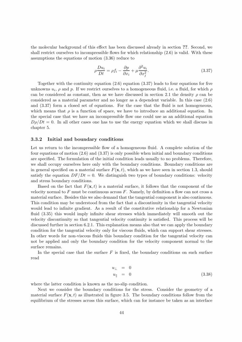
the molecular background of this effect has been discussed already in section ??. Second, weshall restrict ourselves to incompressible flows for which relationship (2.6) is valid. With theseassumptions the equations of motion (3.36) reduce to

ρDui

Dt= ρfi − ∂p

∂xi+ µ

∂2ui

∂x2j

. (3.37)

Together with the continuity equation (2.6) equation (3.37) leads to four equations for fiveunknowns ui, ρ and p. If we restrict ourselves to a homogeneous fluid, i.e. a fluid, for which ρcan be considered as constant, then as we have discussed in section 2.1 the density ρ can beconsidered as a material parameter and no longer as a dependent variable. In this case (2.6)and (3.37) form a closed set of equations. For the case that the fluid is not homogeneous,which means that ρ is a function of space, we have to introduce an additional equation. Inthe special case that we have an incompressible flow one could use as an additional equationDρ/Dt = 0. In all other cases one has to use the energy equation which we shall discuss inchapter 5.

3.3.2 Initial and boundary conditions

Let us return to the incompressible flow of a homogeneous fluid. A complete solution of thefour equations of motion (2.6) and (3.37) is only possible when initial and boundary conditionsare specified. The formulation of the initial condition leads usually to no problems. Therefore,we shall occupy ourselves here only with the boundary conditions. Boundary conditions arein general specified on a material surface F (x, t), which as we have seen in section 1.3, shouldsatisfy the equation DF/Dt = 0. We distinguish two types of boundary conditions: velocityand stress boundary conditions.

Based on the fact that F (x, t) is a material surface, it follows that the component of thevelocity normal to F must be continuous across F . Namely, by definition a flow can not cross amaterial surface. Besides this we also demand that the tangential component is also continuous.This condition may be understood from the fact that a discontinuity in the tangential velocitywould lead to infinite gradient. As a result of the constitutive relationship for a Newtonianfluid (3.35) this would imply infinite shear stresses which immediately will smooth out thevelocity discontinuity so that tangential velocity continuity is satisfied. This process will bediscussed further in section 6.2.1. This explanation means also that we can apply the boundarycondition for the tangential velocity only for viscous fluids, which can support shear stresses.In other words for non-viscous fluids this boundary condition for the tangential velocity cannot be applied and only the boundary condition for the velocity component normal to thesurface remains.

In the special case that the surface F is fixed, the boundary conditions on such surfaceread

u⊥ = 0u‖ = 0 (3.38)

where the latter condition is known as the no-slip condition.Next we consider the boundary conditions for the stress. Consider the geometry of a

material surface F (x, t) as illustrated in figure 3.5. The boundary conditions follow from theequilibrium of the stresses across this surface, which can for instance be taken as an interface

44

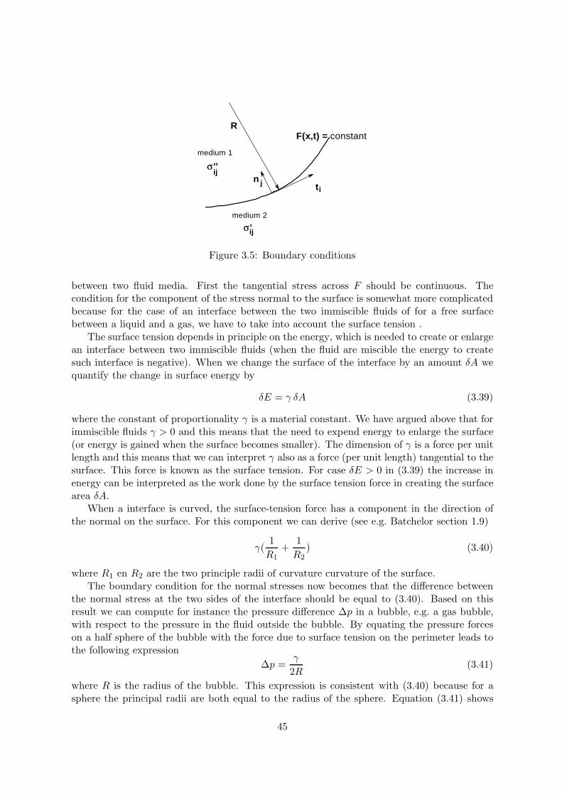
F(x,t) = constant

medium 1

medium 2

R

nt

ij

ij

σ ''

σ '

ij

Figure 3.5: Boundary conditions

between two fluid media. First the tangential stress across F should be continuous. Thecondition for the component of the stress normal to the surface is somewhat more complicatedbecause for the case of an interface between the two immiscible fluids of for a free surfacebetween a liquid and a gas, we have to take into account the surface tension .

The surface tension depends in principle on the energy, which is needed to create or enlargean interface between two immiscible fluids (when the fluid are miscible the energy to createsuch interface is negative). When we change the surface of the interface by an amount δA wequantify the change in surface energy by

δE = γ δA (3.39)

where the constant of proportionality γ is a material constant. We have argued above that forimmiscible fluids γ > 0 and this means that the need to expend energy to enlarge the surface(or energy is gained when the surface becomes smaller). The dimension of γ is a force per unitlength and this means that we can interpret γ also as a force (per unit length) tangential to thesurface. This force is known as the surface tension. For case δE > 0 in (3.39) the increase inenergy can be interpreted as the work done by the surface tension force in creating the surfacearea δA.

When a interface is curved, the surface-tension force has a component in the direction ofthe normal on the surface. For this component we can derive (see e.g. Batchelor section 1.9)

γ(1R1

+1R2

) (3.40)

where R1 en R2 are the two principle radii of curvature curvature of the surface.The boundary condition for the normal stresses now becomes that the difference between

the normal stress at the two sides of the interface should be equal to (3.40). Based on thisresult we can compute for instance the pressure difference ∆p in a bubble, e.g. a gas bubble,with respect to the pressure in the fluid outside the bubble. By equating the pressure forceson a half sphere of the bubble with the force due to surface tension on the perimeter leads tothe following expression

∆p =γ

2R(3.41)

where R is the radius of the bubble. This expression is consistent with (3.40) because for asphere the principal radii are both equal to the radius of the sphere. Equation (3.41) shows

45

that the pressure difference for small bubbles becomes very large. As a consequence it is ingeneral very difficult to produce small bubbles (say smaller than ≈ 100 µm for air bubbles inwater).

In the form of an equation the stress boundary conditions now become:

µ1e′′ijnjti = µ2e

′ijnjti

p′′ − 2µ1(e′′ijnjni − 13∆′′) = p′ − 2µ2(e′ijnjni − 1

3∆′) + γ(

1R1

+1R2

) (3.42)

where t is the unit vector tangential to the interface and which at the same time is directed inthe direction of the shear stress. The n has been already denoted is the unit vector normal tothe interface. Furthermore the following relationship is valid njni = δij . For an explanationof the notation we may refer to figure 3.5.

Problem 3.5 Observe that if a flow u is rotation free or irrotational the viscous term in (3.37)is identical equal to zero. This means that potential flows, which are treated in chapter 4 fornon-viscous fluids, are also a solution of the full Navier-Stokes equations. Does this contradictthe assumption, which we have made for potential flows that they are in principle valid fornon-viscous fluids?

3.3.3 Non-inertial coordinate system

Until now we have assumed that our coordinate system is inertial, i.e. a flow in rest or in auniform constant motion does not experience any accelerations. Let us turn now to a non-inertial system and consider how the Navier-Stokes equations derived in section 3.3.1 aremodified in that case.

First, we consider a coordinate system that experiences a linear acceleration f with respectto a inertial system. Let us denote the velocity in the inertial coordinate system by v andin the non-inertial system by v′. The accelerations of fluid elements in the two coordinatesystems are then connected by the expression

DvDt

=Dv′

Dt+ f . (3.43)

Substitution of (3.37) for Dv/Dt then leads to the equation of motion in the acceleratingcoordinate system. The main result is that on the right-hand of the Navier-Stokes equationan additional acceleration equal to −f appears, which is sometimes also denoted as a virtualforce.

Second, we consider a coordinate system that rotates with respect to an inertial systemwith an angular velocity vector Ω. In this case the relation between the velocity v in theinertial coordinate system and v′ in the rotating system reads

v = v′ + Ω × r (3.44)

where r is the location vector which runs from the position where the velocity is consideredto the rotation axis such that dr/dt = v. To obtain the relationship between the accelerationof fluid elements in the two coordinate systems we must again take the material derivative of(3.44). However, in this case we must take into account that the unit vectors in the rotatingsystem also change as a function of time. This leads to

DvDt

=Dv′

Dt+ Ω × v′ + Ω × v (3.45)

46

where the second term on the right-hand side expresses the contribution due to the rotationof the unit vectors. Substitution of v from (3.44) then gives

DvDt

=Dv′

Dt+ 2Ω × v′ + Ω × (Ω × r) (3.46)

The first term on the right-hand side of this equation is the acceleration of a fluid element inthe rotating coordinate system. The second term is known as the Coriolis acceleration and thecombination 2 |Ω| is called the Coriolis parameter. The last term on the right-hand side is thecentrifugal acceleration. For a homogeneous fluid with constant density and no free surfacesthe contribution by the centrifugal acceleration can be absorbed into pressure term, which isthen called the modified pressure

Finally, substitution of (3.37) for Dv/Dt then leads to the equation of motion in therotating coordinate system.

3.4 Vorticity dynamics

When we will consider the flow of viscous fluids in chapter 6, we shall see that the ‘no-slip’condition can be interpreted as a source of vorticity. In anticipation on this discussion weconsider here the dynamics of vorticity.

We have defined in 2.4.2 a vortex line as a line which is everywhere tangent to the vorticityvector ω and a vortex tube as a cylindrical geometry, of which the side walls consist of vortexlines. The strength of the vortex tube is given by κ defined by (2.44) and we have foundthat this strength of a vortex tube is everywhere the same along the tube. From this wehave concluded that a vortex tube can not end in the flow. This result is also called thefirst Helmholtz vorticity theorem. These properties could be denoted as the kinematics of avorticity field.

Let us now consider the consequences of the equations of motion derived in the previoussections for the dynamics of the vorticity. Let us direct our attention in the first place to theκ, i.e. the strength of a vortex tube, which as we have seen in section 2.4.2 is also called thecirculation as given by (2.45).

Let us now compute how this circulation changes as a function of time or alternatively wedetermine Dκ/Dt. The use of the material derivative is based on the fact that the curve Γ,along which the circulation is computed, is a material curve. It then follows

Dκ

Dt=

D

Dt

∮Γui∂xi

∂sds

=∮

Γ

Dui

Dt

∂xi

∂sds +

∮Γui∂2xi

∂s∂tds

=∮

Γ

Dui

Dt

∂xi

∂sds +

∮Γui∂ui

∂sds

=∮

Γ

Dui

Dt

∂xi

∂sds +

∮Γd12u2

i (3.47)

where we have used the definition that ∂xi/∂t = ui. The velocity field is single valued andthis means that the second contribution on the right-hand side of (3.47) is identically equal tozero. Substitution of the equations of motion (3.37) in the first term on the right-hand side of

47

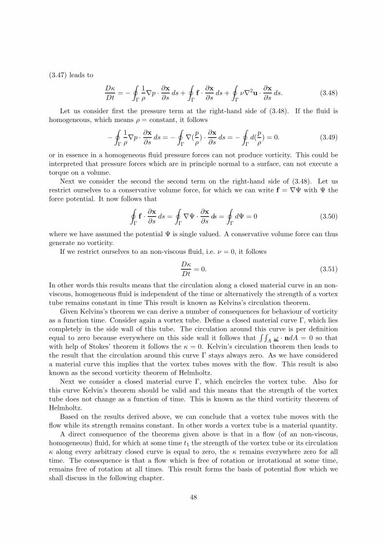
(3.47) leads to

Dκ

Dt= −

∮Γ

1ρ∇p · ∂x

∂sds+

∮Γf · ∂x

∂sds+

∮Γν∇2u · ∂x

∂sds. (3.48)

Let us consider first the pressure term at the right-hand side of (3.48). If the fluid ishomogeneous, which means ρ = constant, it follows

−∮

Γ

1ρ∇p · ∂x

∂sds = −

∮Γ∇(

p

ρ) · ∂x∂s

ds = −∮

Γd(p

ρ) = 0. (3.49)

or in essence in a homogeneous fluid pressure forces can not produce vorticity. This could beinterpreted that pressure forces which are in principle normal to a surface, can not execute atorque on a volume.

Next we consider the second the second term on the right-hand side of (3.48). Let usrestrict ourselves to a conservative volume force, for which we can write f = ∇Ψ with Ψ theforce potential. It now follows that∮

Γf · ∂x

∂sds =

∮Γ∇Ψ · ∂x

∂sds =

∮ΓdΨ = 0 (3.50)

where we have assumed the potential Ψ is single valued. A conservative volume force can thusgenerate no vorticity.

If we restrict ourselves to an non-viscous fluid, i.e. ν = 0, it follows

Dκ

Dt= 0. (3.51)

In other words this results means that the circulation along a closed material curve in an non-viscous, homogeneous fluid is independent of the time or alternatively the strength of a vortextube remains constant in time This result is known as Kelvins’s circulation theorem.

Given Kelvins’s theorem we can derive a number of consequences for behaviour of vorticityas a function time. Consider again a vortex tube. Define a closed material curve Γ, which liescompletely in the side wall of this tube. The circulation around this curve is per definitionequal to zero because everywhere on this side wall it follows that

∫ ∫A ω · ndA = 0 so that

with help of Stokes’ theorem it follows the κ = 0. Kelvin’s circulation theorem then leads tothe result that the circulation around this curve Γ stays always zero. As we have considereda material curve this implies that the vortex tubes moves with the flow. This result is alsoknown as the second vorticity theorem of Helmholtz.

Next we consider a closed material curve Γ, which encircles the vortex tube. Also forthis curve Kelvin’s theorem should be valid and this means that the strength of the vortextube does not change as a function of time. This is known as the third vorticity theorem ofHelmholtz.

Based on the results derived above, we can conclude that a vortex tube moves with theflow while its strength remains constant. In other words a vortex tube is a material quantity.

A direct consequence of the theorems given above is that in a flow (of an non-viscous,homogeneous) fluid, for which at some time t1 the strength of the vortex tube or its circulationκ along every arbitrary closed curve is equal to zero, the κ remains everywhere zero for alltime. The consequence is that a flow which is free of rotation or irrotational at some time,remains free of rotation at all times. This result forms the basis of potential flow which weshall discuss in the following chapter.

48

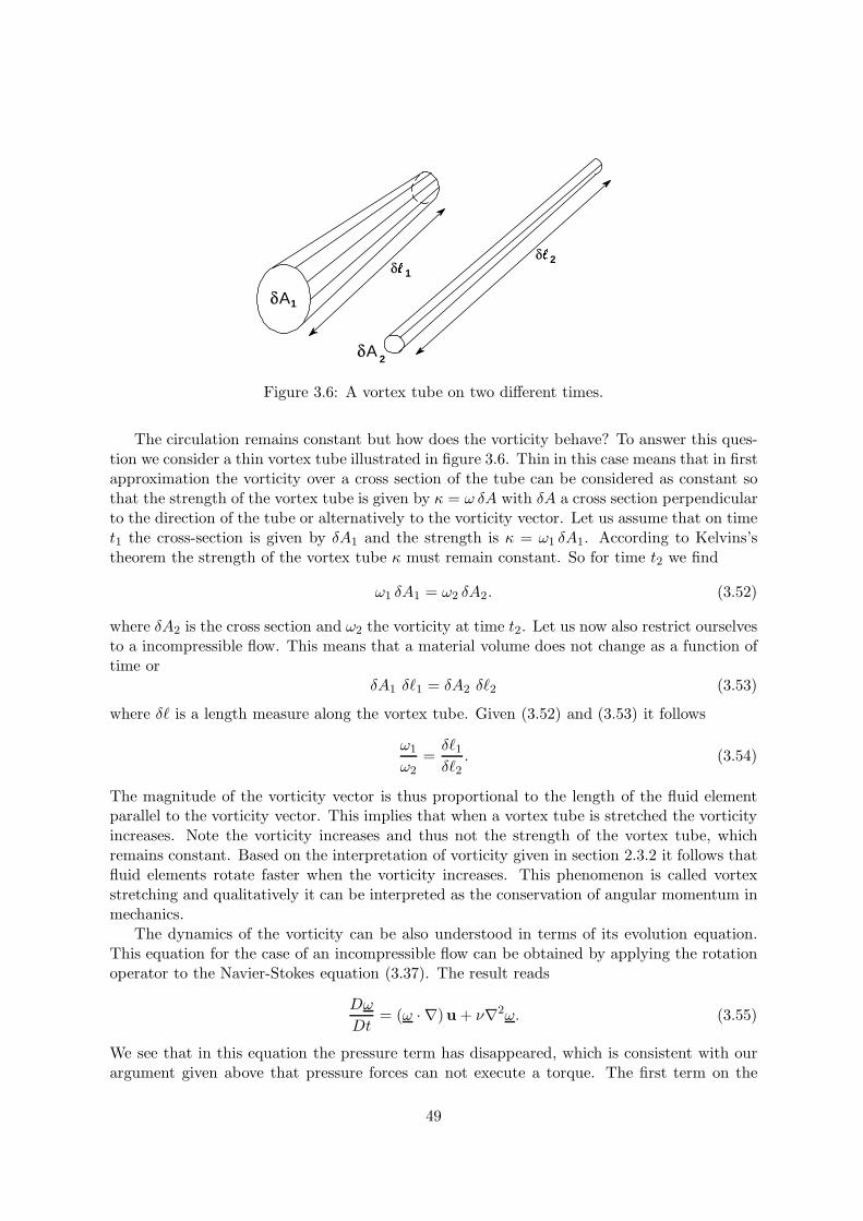
δA1

δA 2

δ

δ

12

Figure 3.6: A vortex tube on two different times.

The circulation remains constant but how does the vorticity behave? To answer this ques-tion we consider a thin vortex tube illustrated in figure 3.6. Thin in this case means that in firstapproximation the vorticity over a cross section of the tube can be considered as constant sothat the strength of the vortex tube is given by κ = ω δA with δA a cross section perpendicularto the direction of the tube or alternatively to the vorticity vector. Let us assume that on timet1 the cross-section is given by δA1 and the strength is κ = ω1 δA1. According to Kelvins’stheorem the strength of the vortex tube κ must remain constant. So for time t2 we find

ω1 δA1 = ω2 δA2. (3.52)

where δA2 is the cross section and ω2 the vorticity at time t2. Let us now also restrict ourselvesto a incompressible flow. This means that a material volume does not change as a function oftime or

δA1 δ1 = δA2 δ2 (3.53)

where δ is a length measure along the vortex tube. Given (3.52) and (3.53) it follows

ω1

ω2=δ1δ2

. (3.54)

The magnitude of the vorticity vector is thus proportional to the length of the fluid elementparallel to the vorticity vector. This implies that when a vortex tube is stretched the vorticityincreases. Note the vorticity increases and thus not the strength of the vortex tube, whichremains constant. Based on the interpretation of vorticity given in section 2.3.2 it follows thatfluid elements rotate faster when the vorticity increases. This phenomenon is called vortexstretching and qualitatively it can be interpreted as the conservation of angular momentum inmechanics.

The dynamics of the vorticity can be also understood in terms of its evolution equation.This equation for the case of an incompressible flow can be obtained by applying the rotationoperator to the Navier-Stokes equation (3.37). The result reads

Dω

Dt= (ω · ∇)u + ν∇2ω. (3.55)

We see that in this equation the pressure term has disappeared, which is consistent with ourargument given above that pressure forces can not execute a torque. The first term on the

49

right-hand side of (3.55) gives the change of vorticity as a result of deformation in the flowfield. It describes for instance the process of vortex stretching, which we have discussed above.

We have thus found that in contrast to the circulation the vorticity itself can change underthe influence of deformations of the flow field. Furthermore, the equation (3.55) without theviscosity term, is found to be identical to the equation which describes the evolution of amaterial line element δ. It thus follows that the vorticity behaves similarly as a material linesegment which is consistent with the theorems of Helmholtz discussed above.

Let us return to Kelvin’s theorem (3.51). Under which circumstances can the circulationalong a closed material curve change? To answer this question we return to the discussion ofthe individual terms in the equation (3.48). Let us consider again the pressure term. We haveseen that his term disappears for the case of a homogeneous fluid. We can extrapolate thisresult to a so-called barotropic fluid, which is a fluid that satisfies an equation of state givenby p = f(ρ). For an arbitrary medium p =/ f(ρ) but rather p = f(ρ, T ). Such a medium iscalled a baroclinic fluid and in this case the pressure term does not disappear. The change ofthe circulation is now given by

Dκ

Dt= −

∮Γ

1ρ∇p · ds. (3.56)

This equation plays an important role in a description of atmospheric flows and in this contextit is also called the theorem of Bjerknes.

Another process to change the circulation around a closed material curve is by means ofviscosity as described by the last term in (3.48). The effect of viscosity and its interpretationin terms of vorticity will be discussed further in chapter 6.

Problem 3.6 The helicity of a material volume V of fluid is defined as

H =∫ ∫ ∫

Vu · ω dV

where the integral is taken over the whole volume. Show that under the condition ω · n = 0on the surface A of V the helicity H is conserved.

Problem 3.7 Consider the vorticity equation (3.55) for an inviscid fluid, i.e. ν = 0. Take thescalar product of ω with ∇λ where λ (x, t) is any scalar function of position and time. Showthat

D

Dtω · ∇λ = (ω · ∇)

Dλ

Dt

this result is known as Ertel’s theorem.

Problem 3.8 Consider the Lagrangian description of the following flow with position coordi-nates X = (X1,X2,X3) as a function of time t given by:

X1 = e−12αt

[a1 cos

Ωα

(eαt − 1

)− a2 cos

Ωα

(eαt − 1

)]

X2 = e−12αt

[a2 cos

Ωα

(eαt − 1

)+ a1 cos

Ωα

(eαt − 1

)]X3 = a3e

αt

50

where (a1, a2, a3) is the position of the particle at t = 0 and where α is a constant. Show thatthe velocity field is given by:

u =(−1

2αx− Ωyeαt,−1

2αy + Ωxeαt, αz

)

Compute the rate of deformation tensor and the vorticity vector. Show that the vorticityequation (3.55) is satisfied.

Problem 3.9 Obtain an exact solution to the Navier-Stokes equations in cylindrical coordi-nates with a velocity field given by

u = (ur, uφ, uz) =(− 1

2αr, uφ(r), αz

)

where α is a positive constant. Show that

uφ =Γ

2πr

(1 − e−

αr2

4ν

)

ωr = 0, ωφ = 0, ωz = Γα

4πνe−

αr2

4ν

where Γ is an arbitrary constant with the dimensions [m2 s−1]. This result is known as theBurgers vortex. Show that Γ is the circulation of this vortex.

Problem 3.10 Let a fluid element be at t = 0 at the position a with a value of the vorticityat this position equal to ω0. Consider the motion of an non-viscous fluid in a Lagrangian frameof reference, i.e. given is the trajectory X(t;a) of the fluid element. Show that

ωi = ω0j

∂Xi

∂aj.

This result is known as Cauchy’s vorticity equation.

Problem 3.11 Show that for an ideal fluid the vorticity equation can be written as

∂ω

∂t= ∇× [u× ω]

and that for a rotating coordinate system with the rotation vector Ω this equation can beextended to

∂ (ω + 2Ω)∂t

= ∇× [u × (ω + 2Ω)] .

Show that for a stationary flow this leads to

(Ω · ∇)u = 0.

Interpret this result, which is known as the Taylor-Proudman theorem. What are the conse-quences for the velocity components perpendicular to the Ω vector.

51

Problem 3.12 Derive for a stationary flow of a viscous fluid the expression

ν

∮C

(∇× ω) · ds = 0

with ω = ∇×u and C a closed streamline. Next consider a two-dimensional flow, which impliesthat ω has only one component unequal to zero. Show with help of the result of problem 6.1 foran ideal fluid (i.e. for ν = 0 and for a stationary, two-dimensional flow it follows that ω = ω (ψ)where ψ is the stream function) that

dω

dψ

∮C

u · ds = 0

which implies that in the limit ν → 0 the ω should be constant in any region of with closedstreamlines. This is known as the Batchelor-Prandtl theorem.

52

Chapter 4

Non-viscous fluids: potential flow

4.1 Euler-equations

For many fluids, like air and water, the viscosity seems negligibly small. As a first approxi-mation we may then neglect the effect of viscosity on the flow. Note, that at this stage wecan make this approximation only in a qualitative sense. Only in chapter 6 we shall see howto quantify the effect of viscosity and also under what conditions the neglect of viscosity isjustifiable.

Let us start in this chapter by making the perhaps bold assumption that the viscosity canbe set to zero or µ = 0. In this case one speaks of an ideal fluid. For an incompressible flowand a homogeneous fluid the Navier-Stokes equations (3.37) then reduce to

ρDui

Dt= ρfi − ∂p

∂xi. (4.1)

and this equation is known as the Euler equation. Together with the continuity equation (2.6)it forms the governing equation for the flow of an ideal, non-viscous fluid or alternatively aninviscid flow.

An important difference with the full Navier-Stokes equations (3.37) is the fact that theEuler equations are of a lower order. Namely, the second-order derivatives in (3.37) havedisappeared. This has as consequence that for the solution of the Euler equations one needsone boundary condition less than for the Navier-Stokes equations to specify a solution, i.e. oneboundary condition instead of two. In section 3.3.1 we have seen that in an non-viscous fluidwe can not specify a condition for the tangential velocity or the tangential stress. In otherwords the no-slip condition can no longer be satisfied.

Problem 4.1 Consider on a flat horizontal surface a shallow layer of water with a constantdensity ρ0 and with a depth H(x, y, t). Assume that the scale of the flow motions in thislayer are much larger than the depth. As a result we may approximate the flow in the shallowlayer as two-dimensional with the velocity vector u with the components (u, v) in the twohorizontal directions parallel to the surface. In other words the vertical velocity componentmay be neglected. The pressure above the free surface is assumed to be constant and equalto p0. Formulate by integrating the continuity equation (2.6) and the Euler equations (4.1)(which should include the contribution due to gravity) across the layer in the vertical direction

53

the following equations for H and u

DH

Dt= −H∇H · u

DuDt

= −ρ0gH ∇HH

where ∇H is the horizontal nabla operator given by ∇H = (∂ /∂x, ∂ /∂y). These equationsare known as the shallow water equations.

Problem 4.2 Consider a shallow layer of water above a flat surface. Initially, the depthH = H0 is constant and the water is quiescent, i.e. u = 0. Assume a small disturbance H ′ onH0 such that H ′/H0 1. By linearising the shallow water equations derived in problem 4.1,show that the equation for H ′ becomes

∂2H ′

∂t2= ρgH0

(∂2H ′

∂x2+∂2H ′

∂y2

).

Interpret the solution of this equation.

Problem 4.3 Show that the shallow water equations derived in problem 4.1 lead to the fol-lowing vorticity equation.

D

Dt

( ωH

)= 0,

where ω = ∂v/∂x − ∂u/∂y. The ratio ω/H is known as the potential vorticity.

Problem 4.4 Formulate the shallow water equations of problem 4.1 in a rotating frame ofreference and show that in that case the equation for the potential vorticity becomes equal to

D

Dt

(ω + f

H

)= 0,

where ω is defined as in 4.3 and f is the Coriolis parameter, which is equal to f = 2Ω whereΩ in this case is the component of the angular velocity vector parallel to the direction of theacceleration of gravity. The sum ω + f is called in this case the absolute vorticity and the ωthe relative vorticity.

Problem 4.5 Consider the equivalent to problem 4.2 for a depth disturbance on a constantwater depth H0 but now for the shallow water equations in a rotating frame of reference. Inthat case a stationary solution is possible. Show that the horizontal size of this stationarydisturbance is proportional to

Rb ∝√gH0

f,

where Rb is called the Rossby radius of deformation and f is the Coriolis parameter.

Problem 4.6 Consider in a shallow water layer two vertically oriented, free vortices at adistance D from each other and with opposite rotation directions. The problem is comparablewith the two point vortices which we have considered in section 2.4.2 in equations (2.50) and(2.51) and we consider for convenience that the two vortices can be represented by pointvortices with strength κ and −κ, respectively. When the water depth is constant the two

54

vortices propagate similarly as found in section 2.4.2 along a linear trajectory perpendicularto their separation vector. However, assume now that the depth H varies according to

H = H0 − δHx2

L2 + 1

with δH H0 and L H0. The two vortices approach this depth variation. By applying theconcept of potential vorticity considered in problem 4.3 compute the path of the two vorticesas a function of the angle of the separation vector D with the y-axis.

Problem 4.7 Consider a shallow water layer in a rotating frame of reference with a Coriolisparameter f , which in this case varies according to

f = f0 + βy

with β > 0. This variation of the Coriolis parameter is known as the β-plane approximationand it represents as a first approximation the variation of f as a function of latitude alongthe earth’s surface. A single vertically oriented, free vortex propagates along the x-axis with aspeed U . Like in problem 4.6 the vortex can be considered as a point vortex with strength κ.The vortex approaches a similar depth variation as considered in problem 4.6. Compute thetrajectory of the vortex both for case that the vortex initially moves in the positive x-directionand for the case that the vortex initially moves in the negative x-direction. Consider also thetwo cases for a positive and negative value of κ. (Apply the potential vorticity equation derivedin problem 4.4.)

Problem 4.8 Consider a pair of free vortices with opposite rotation and at a distance d fromeach other. The vortices approach a cylinder with radius a. Compute the trajectories of thesevortices (make use of the result derived in problem 2.17 for the case of a non-viscous fluid.Discuss qualitatively the result for a viscous fluid.

4.2 Rotation-free flows

Let us now restrict ourselves to the case where the vorticity is zero everywhere in the flow,i.e. ∇ × u = 0. These are called rotation free flows. For the case of the non-viscous fluidsconsidered here, we can make use of Kelvin’s theorem (3.51), which we have proved in section3.4. Based on this theorem it follows that a flow, which is initially rotation free, stays rotationfree for all time. In other words a rotation free flow field is a realisable solution of the Eulerequations. As example we mention the important class of solutions for all flows which startfrom a situation of rest, i.e. u = 0. The initial condition in that case satisfies trivially thecondition of a rotation free flow field.

In addition to ∇ × u = 0 we must also the continuity equation (2.6): ∇ · · ·u = 0 foran incompressible flow. If we remember the Helmholtz decomposition, which we discussed insection 2.4, this means that we are now considering the last contribution in this decomposition(2.24).

In addition it should be mentioned that the rotation free flow field which is found as solutionof the Euler equations (4.1) , is also a solution of the full Navier-Stokes equations (3.37).However, this solution does not necessarily satisfy the correct boundary condition, which asolution of the Navier-Stokes equations should satisfy. This is in particular the case for the

55

no-slip condition. Only in those cases where the no-slip plays a minor role, e.g. on the interfacebetween two fluids, can the rotation free solution of the Euler equations be interpreted as afirst approximation to the full solutions of the Navier-Stokes equations. A well-known exampleis the flow of a liquid around a gas bubble.

It will become clear below that with the class of rotation and divergence free flow fields wecan solve a large number of practical flow problems.

4.2.1 Potential flows: general properties

In section 2.4.1 we have already seen that the condition of a rotation free velocity field can besatisfied by the introduction of a velocity potential Φ according to

u = grad Φ (4.2)

and the resulting flows are called potential flows.Substitution of (4.2) in the continuity equation (2.6) then leads to the following equation

for Φ∇2Φ = 0. (4.3)

This equation is known as the Laplace equation. The general solution of the Laplace equationis called a harmonic function.

For the boundary conditions of the solution of Laplace’s equation (4.3) we chose a conditionfor the velocity. Because we consider here non-viscous fluids we can only specify a conditionfor the normal component of the velocity on a material surface (see section 3.3.2). This meansthat on the (material) surface A of a our flow region the gradient of Φ in the direction of thenormal is given, or ∂Φ/∂n is given. In this form the solution of the Laplace equations is calledthe Neumannn problem. The use of this boundary condition implies that the flow potential iscan be only determined apart from an arbitrary constant, which in principle may be a functionof time.

Some examples of potential flows are

Φ = Uixi (4.4)Φ = α(x2 − y2). (4.5)

The first potential represents a flow with a constant velocity vector Ui or in other words aparallel flow. The second potential is a pure straining flow in two dimensions. For this caseone can compute that the only components of the deformation tensor eij that are not equalto zero, are the e11 and the e22 component, which are equal to α and −α, respectively. Thex− and y−axis are thus the principal axes. Line segments along the x−axis are stretched andline segments along the y−axis are compressed. In the origin, x = 0 and y = 0, the velocity isequal to zero. Therefore another name for this case is a stagnation flow.

Another example of a potential flow is the source solution (2.30), which we have discussedin some detail in section 2.4.1. To consider this flow as a solution of the Laplace equation weneed of course to exclude the singularity at the source location from our flow region, becauseat this location the condition of a divergence free flow field is not satisfied. This result can ofcourse be extended to the other solutions of the Poisson equation, which we have derived in2.4.1. However, once more we must restrict ourselves to the flow region outside the singularitiesor alternatively to those regions where the right-hand side of the Poisson equation is equal tozero.

56

The equation of Laplace (4.3) is linear. This has the advantage that we can make use ofthe extensive mathematical theory for linear differential equations. One of the results of thistheory is the superposition principle: i.e. the sum of two solutions is again a solution. Thishas been applied before in section 2.4.1 to derive the dipole flow (2.38). The dipole flow canthus also be interpreted as a potential flow and in this case the flow is everywhere divergencefree even at the location of the dipole. In this chapter we shall make use of the superpositionprinciple to compute other flows.

Until now we have restricted ourselves to the solution of the Laplace equation for thevelocity field which satisfies the continuity equation (2.6) and at the same time is rotation free.This can be considered as a kinematic description of the flow field such as we have consideredin section 2.4. The dynamics, which in this case is given by the Euler equations, has been leftaside until now. However, for the case of a potential flow the Euler equations can be integratedexactly and the resulting relationship can be used to compute the pressure field. To this endwe rewrite the Euler equations (4.1) with help of the relation (A.16) as

∂u∂t

− u× ω + ∇ ·(

12u2

)= ∇

(− p

ρ+ g · x

)(4.6)

where we have substituted for the volume force f acceleration of gravity g = (0, 0,−g). Gravityis a conservative body force with a force potential Ψ = g · x so that g = ∇Ψ where Ψ can bealso interpreted as an potential energy (per unit mass). With help of (4.2) and the fact thatω ≡ ∇× u = 0 it follows from the (4.6) that

∇(∂Φ∂t

+12u2 +

p

ρ+ gz) = 0

∂Φ∂t

+12u2 +

p

ρ+ gz = C (4.7)

where the C is a constant which may be a function if time. This equation is know as the lawof Bernouilli for a potential flow. In chapter 5 we shall encounter an alternative formulation ofthe law of Bernouilli by considering the conservation of energy of the flow. Apart for the staticpressure the term 1/2u2 in (4.7) is sometimes called the dynamic pressure. If we neglect thegravity term, (4.7) shows that the maximum static pressure occurs at the position where thevelocity is zero, i.e. in a so-called stagnation point. For that reason this maximum pressure issometimes called the stagnation pressure .

With the results, that we have obtained for potential flows until now, we can describenow in general terms how a potential flow problem can be solved. With help of (4.3) and theboundary conditions for the normal component of the velocity we can compute the velocityfield. Based on this velocity field and the law of Bernouilli we can subsequently derive thepressure field. This pressure field can then for instance be used to compute the forces on abody.

To end this section we state a number of general properties of potential flows, which areproven in appendix D for a so-called singly-connected region. To define a singly-connectedregion we consider the volume V illustrated in figure 4.1. The volume is bounded by an outersurface A2 with the outside pointing normal n2 and by an inner surface A1 with the inwardpointing normal n1. This volume V is a singly-connected region because the following tworequirements are satisfied:

57

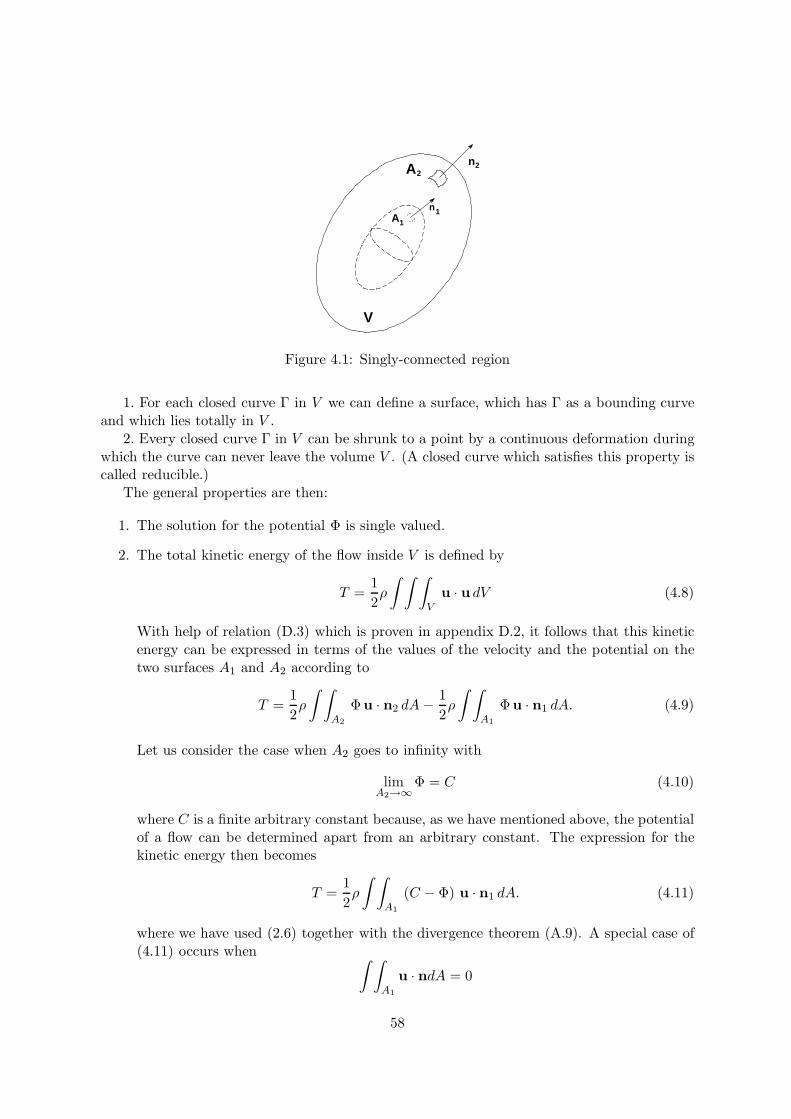
V

An

A1

2

n1

2

Figure 4.1: Singly-connected region

1. For each closed curve Γ in V we can define a surface, which has Γ as a bounding curveand which lies totally in V .

2. Every closed curve Γ in V can be shrunk to a point by a continuous deformation duringwhich the curve can never leave the volume V . (A closed curve which satisfies this property iscalled reducible.)

The general properties are then:

1. The solution for the potential Φ is single valued.

2. The total kinetic energy of the flow inside V is defined by

T =12ρ

∫ ∫ ∫V

u · u dV (4.8)

With help of relation (D.3) which is proven in appendix D.2, it follows that this kineticenergy can be expressed in terms of the values of the velocity and the potential on thetwo surfaces A1 and A2 according to

T =12ρ

∫ ∫A2

Φu · n2 dA− 12ρ

∫ ∫A1

Φu · n1 dA. (4.9)

Let us consider the case when A2 goes to infinity with

limA2→∞

Φ = C (4.10)

where C is a finite arbitrary constant because, as we have mentioned above, the potentialof a flow can be determined apart from an arbitrary constant. The expression for thekinetic energy then becomes

T =12ρ

∫ ∫A1

(C − Φ) u · n1 dA. (4.11)

where we have used (2.6) together with the divergence theorem (A.9). A special case of(4.11) occurs when ∫ ∫

A1

u · ndA = 0

58

which means that the volume transport through the closed surface A1 is equal to zero,which for instance applies to the flow around a solid body. In that case we find for thekinetic energy

T = −12ρ

∫ ∫A1

Φu · n1 dA. (4.12)

3. The solution for a potential flow is unique apart from an additive constant.

4. The kinetic energy of a potential flow is minimal for all possible flow solutions in thesingly-connected region V that satisfy the same boundary conditions on the boundingsurfaces of the region.

5. The potential can not have a maximum value in side V . This implies that the maximumvalue of the absolute velocity must always occur on the boundary of the region V . Asa result of the law of Bernouilli this means also that the minimal pressure must alsooccur only on the boundary of the flow region. (Note these results are only valid for themaximum flow speed and the minimal pressure. The minimal flow speed, which is equalto 0, and thus the maximum pressure can occur inside the flow domain.)

In flow of liquids such as water, regions with minimal pressure pressure can sometimesbecome very small or even negative, where a negative pressure means that the fluid isunder a tensile strain. The fluid can not support these tensile stresses and as a resultbubbles appear with gases that have been dissolved in liquid. A frequently occurringcondition in practice, however, is when the pressure becomes lower then the vapourpressure of the liquid. In that case vapour bubbles appear. This phenomenon is calledcavitation. In other words the fluid starts to boil locally. However we have argued insection 3.3.2 that it is difficult for small bubbles to survive because of the high pressuredifference that is needed to keep the bubble in equilibrium with the fluid outside thebubble. Therefore, cavitation usually starts from small air bubbles, which are presentwithin the fluid or within cracks in a wall.

Based on the results discussed above, it seems that appearance of cavitation can be firstexpected on the boundary of the flow region or on the surface of the body. An unpleasantcircumstance is that cavitation near the surface of a body may lead to a lot of damage,especially when the vapour bubbles implodes in region of the flow where the pressurebecomes higher than the vapour pressure.

Problem 4.9 Formulate the equivalent of the stagnation flow (4.5) for an axi-symmetricalflow geometry. Compute the potential and the stream function.

4.3 Three-dimensional potential flows

4.3.1 Flow from a container

First we consider a example of potential flow without computing the velocity field in detail.Point of departure is a container as illustrated in figure 4.2. The container is filled with aliquid with density ρ till a height h above the outflow orifice, which has an surface area S. Theflow starts from a state of rest and when we can assume the fluid to be ideal Kelvin’s theorem(3.51) predicts that the flow can be described in terms of a potential flow.

59

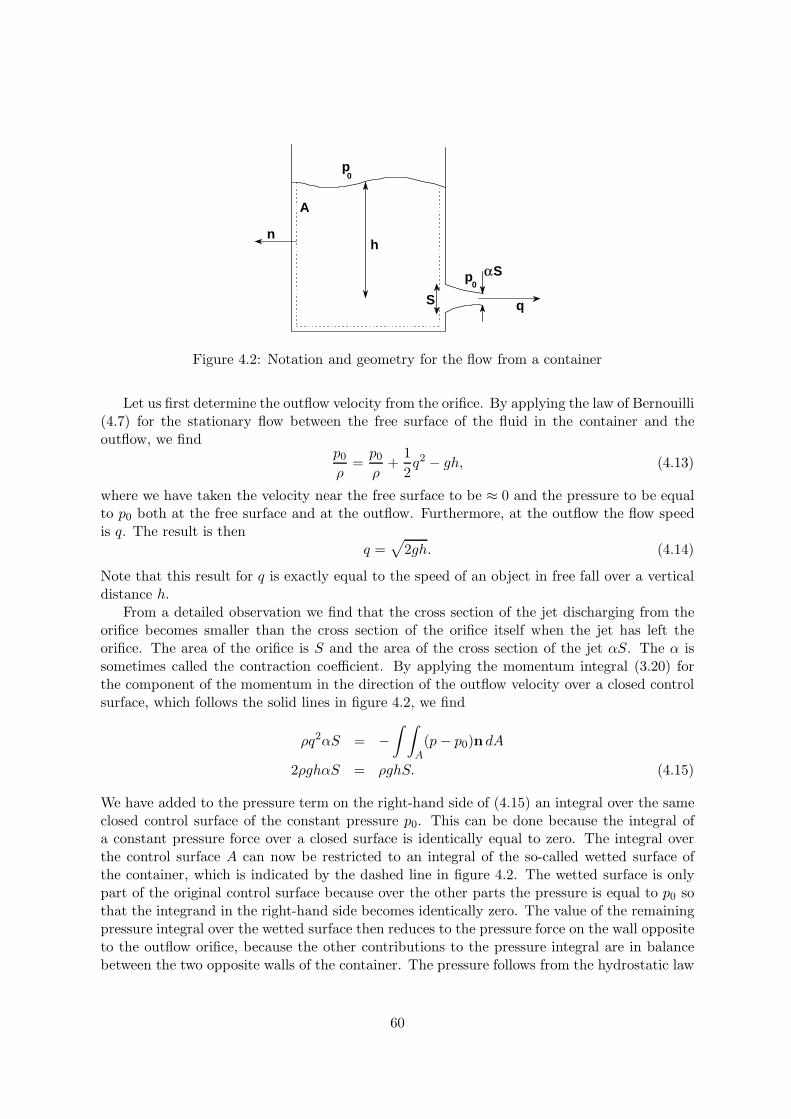
p

p

n

A

αS

S q

h

0

0

Figure 4.2: Notation and geometry for the flow from a container

Let us first determine the outflow velocity from the orifice. By applying the law of Bernouilli(4.7) for the stationary flow between the free surface of the fluid in the container and theoutflow, we find

p0

ρ=p0

ρ+

12q2 − gh, (4.13)

where we have taken the velocity near the free surface to be ≈ 0 and the pressure to be equalto p0 both at the free surface and at the outflow. Furthermore, at the outflow the flow speedis q. The result is then

q =√

2gh. (4.14)

Note that this result for q is exactly equal to the speed of an object in free fall over a verticaldistance h.

From a detailed observation we find that the cross section of the jet discharging from theorifice becomes smaller than the cross section of the orifice itself when the jet has left theorifice. The area of the orifice is S and the area of the cross section of the jet αS. The α issometimes called the contraction coefficient. By applying the momentum integral (3.20) forthe component of the momentum in the direction of the outflow velocity over a closed controlsurface, which follows the solid lines in figure 4.2, we find

ρq2αS = −∫ ∫

A(p − p0)n dA

2ρghαS = ρghS. (4.15)

We have added to the pressure term on the right-hand side of (4.15) an integral over the sameclosed control surface of the constant pressure p0. This can be done because the integral ofa constant pressure force over a closed surface is identically equal to zero. The integral overthe control surface A can now be restricted to an integral of the so-called wetted surface ofthe container, which is indicated by the dashed line in figure 4.2. The wetted surface is onlypart of the original control surface because over the other parts the pressure is equal to p0 sothat the integrand in the right-hand side becomes identically zero. The value of the remainingpressure integral over the wetted surface then reduces to the pressure force on the wall oppositeto the outflow orifice, because the other contributions to the pressure integral are in balancebetween the two opposite walls of the container. The pressure follows from the hydrostatic law

60

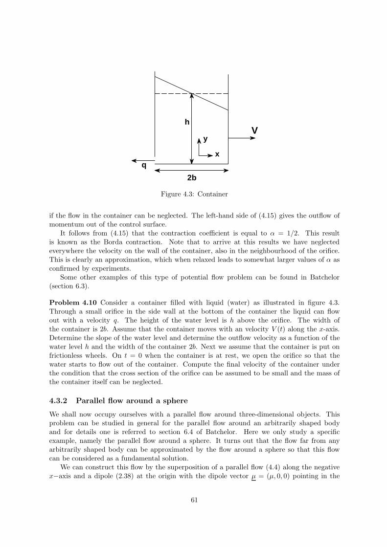
V

x

y

h

q

2b

Figure 4.3: Container

if the flow in the container can be neglected. The left-hand side of (4.15) gives the outflow ofmomentum out of the control surface.

It follows from (4.15) that the contraction coefficient is equal to α = 1/2. This resultis known as the Borda contraction. Note that to arrive at this results we have neglectedeverywhere the velocity on the wall of the container, also in the neighbourhood of the orifice.This is clearly an approximation, which when relaxed leads to somewhat larger values of α asconfirmed by experiments.

Some other examples of this type of potential flow problem can be found in Batchelor(section 6.3).

Problem 4.10 Consider a container filled with liquid (water) as illustrated in figure 4.3.Through a small orifice in the side wall at the bottom of the container the liquid can flowout with a velocity q. The height of the water level is h above the orifice. The width ofthe container is 2b. Assume that the container moves with an velocity V (t) along the x-axis.Determine the slope of the water level and determine the outflow velocity as a function of thewater level h and the width of the container 2b. Next we assume that the container is put onfrictionless wheels. On t = 0 when the container is at rest, we open the orifice so that thewater starts to flow out of the container. Compute the final velocity of the container underthe condition that the cross section of the orifice can be assumed to be small and the mass ofthe container itself can be neglected.

4.3.2 Parallel flow around a sphere

We shall now occupy ourselves with a parallel flow around three-dimensional objects. Thisproblem can be studied in general for the parallel flow around an arbitrarily shaped bodyand for details one is referred to section 6.4 of Batchelor. Here we only study a specificexample, namely the parallel flow around a sphere. It turns out that the flow far from anyarbitrarily shaped body can be approximated by the flow around a sphere so that this flowcan be considered as a fundamental solution.

We can construct this flow by the superposition of a parallel flow (4.4) along the negativex−axis and a dipole (2.38) at the origin with the dipole vector µ = (µ, 0, 0) pointing in the

61

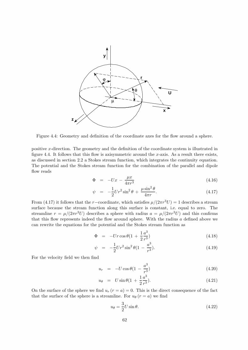
x

z

y

Uθ

ϕ

µ

r

Figure 4.4: Geometry and definition of the coordinate axes for the flow around a sphere.

positive x-direction. The geometry and the definition of the coordinate system is illustrated infigure 4.4. It follows that this flow is axisymmetric around the x-axis. As a result there exists,as discussed in section 2.2 a Stokes stream function, which integrates the continuity equation.The potential and the Stokes stream function for the combination of the parallel and dipoleflow reads

Φ = −Ux − µx

4πr3(4.16)

ψ = −12Ur2 sin2 θ +

µ sin2 θ

4πr. (4.17)

From (4.17) it follows that the r−coordinate, which satisfies µ/(2πr3U) = 1 describes a streamsurface because the stream function along this surface is constant, i.e. equal to zero. Thestreamline r = µ/(2πr3U) describes a sphere with radius a = µ/(2πr3U) and this confirmsthat this flow represents indeed the flow around sphere. With the radius a defined above wecan rewrite the equations for the potential and the Stokes stream function as

Φ = −Ur cos θ(1 +12a3

r3) (4.18)

ψ = −12Ur2 sin2 θ(1 − a3

r3). (4.19)

For the velocity field we then find

ur = −U cos θ(1 − a3

r3) (4.20)

uθ = U sin θ(1 +12a3

r3). (4.21)

On the surface of the sphere we find ur (r = a) = 0. This is the direct consequence of the factthat the surface of the sphere is a streamline. For uθ (r = a) we find

uθ =32U sin θ. (4.22)

62

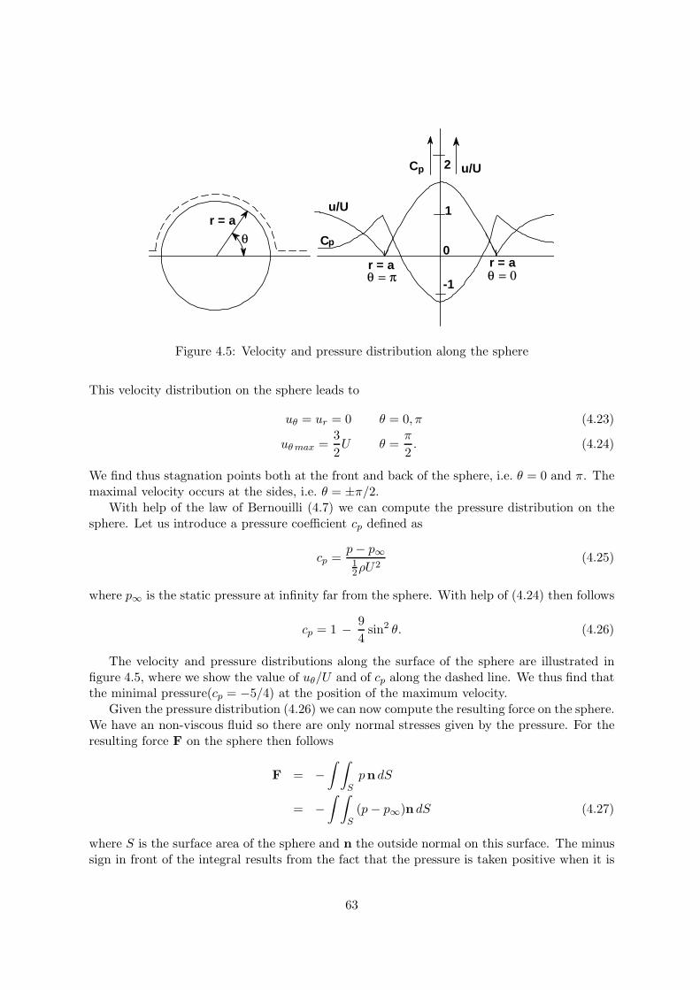
u/U

u/U

C

r = a r = a

1

2

-1

C

p

p

θ = 0θ = π

r = a

θ 0

Figure 4.5: Velocity and pressure distribution along the sphere

This velocity distribution on the sphere leads to

uθ = ur = 0 θ = 0, π (4.23)

uθ max =32U θ =

π

2. (4.24)

We find thus stagnation points both at the front and back of the sphere, i.e. θ = 0 and π. Themaximal velocity occurs at the sides, i.e. θ = ±π/2.

With help of the law of Bernouilli (4.7) we can compute the pressure distribution on thesphere. Let us introduce a pressure coefficient cp defined as

cp =p− p∞12ρU

2(4.25)

where p∞ is the static pressure at infinity far from the sphere. With help of (4.24) then follows

cp = 1 − 94

sin2 θ. (4.26)

The velocity and pressure distributions along the surface of the sphere are illustrated infigure 4.5, where we show the value of uθ/U and of cp along the dashed line. We thus find thatthe minimal pressure(cp = −5/4) at the position of the maximum velocity.

Given the pressure distribution (4.26) we can now compute the resulting force on the sphere.We have an non-viscous fluid so there are only normal stresses given by the pressure. For theresulting force F on the sphere then follows

F = −∫ ∫

Spn dS

= −∫ ∫

S(p− p∞)n dS (4.27)

where S is the surface area of the sphere and n the outside normal on this surface. The minussign in front of the integral results from the fact that the pressure is taken positive when it is

63

directed opposite to the normal. The second step in (4.27) follows from the fact that resultingforce following from integration of a constant pressure over a closed surface is equal to zero.

Let us evaluate (4.27) for the x-component of this resulting force or for the component ofthe force parallel to the flow U . This component of the force is generally called the drag. Withhelp of (4.26) and nx = cos θ we find

Fx = −∫ π

0(p− p∞) cos θ 2πa sin θ adθ

= −πa2ρU2

∫ π

0(1 − 9

4sin2 θ) sin θ cos θdθ

= 0 (4.28)

where we have evaluated the surface integral by means of integrating over circular rings ofmagnitude 2πa sin θ adθ for 0 < θ < π.

The result is thus that the drag is equal to zero. The same result is found for the potentialflow around any arbitrarily shaped body in a parallel flow. The drag being equal to zero isclearly in contradiction with our practical experience. Therefore, this result is usually called aparadox, namely the paradox of d’Alembert. In the following section we return to explain thephysical background of this paradox.

4.3.3 A sphere, moving in an infinite medium

In the previous section we have considered the flow around a sphere where the coordinatesystem was fixed with respect to the sphere. With help of this solution we can also computethe flow around a sphere when the sphere is moving with a velocity U in a quiescent fluid.In other words we consider the flow in a coordinate system that is fixed with respect to thenon-moving fluid at infinity. The potential and the Stokes stream function for this case can befound by subtracting from (4.18) and (4.19) the contribution of the parallel flow with as result

Φ = −12Ua3 cos θ

r2(4.29)

ψ = +12Ua3 sin2 θ

r, (4.30)

i.e. the contribution of the dipole remains. That this result represents indeed the flow arounda moving sphere, can be seen by computing from (4.29) or (4.30) the normal velocity onthe surface of the sphere (note that we have to satisfy the boundary condition only for thenormal component of the velocity). It follows from (4.29) that this velocity component readsur(r = a) = U cos θ. If we remember that the sphere moves in the x-direction with a velocityU , it follows that U cos θ is the projection of this velocity on the normal on the surface of thesphere. So we have satisfied the boundary condition that the normal component on a materialsurface must be continuous. Note, however, that the velocity component tangential to thesurface is not continuous at the surface of the sphere.

In contrast with the stationary flow around the fixed sphere of section 4.3.2 the flow in thepresent case is instationary because as the sphere changes its position in the coordinate system.This implies that the flow at each given point must vary as a function of time. The surfaceof the sphere is a material surface so that each point on the surface carries out a trajectory.Because the flow is now instationary, these trajectories, however, can no longer be interpreted

64

as streamlines. The expressions (4.29) and (4.30) give the potential and the stream function onthe exact moment that the sphere passes the origin of the coordinate system. Let’s define thisinstant as the origin of our time coordinate system, i.e. t = 0. We can now also express (4.29)and (4.30) for an arbitrary time t provided that the r and θ are computed with respect to theposition of the sphere at that time or: r = (x−Ut)2 +y2 +z21/2 and θ = cos−1(x−Ut)/r.Note also, that in an application of the law of Bernouilli (4.7) in this flow one should not forgetthe term ∂Φ/∂t, otherwise we obtain for instance for the pressure distribution on the sphere aresult that is different from (4.26).

Let us now compute for this flow the kinetic energy. We can calculate this energy directlyfrom its definition, which reads

T =12ρ

∫ ∫ ∫V

u · u dV =12ρ

∫ ∫ ∫V

[(∂Φ∂r

)2

+(

1r

∂Φ∂θ

)2]dV (4.31)

where V is the flow volume outside the sphere so that (4.31) can be written as

T =12ρ

∫ 2π

0

∫ π

0

∫ ∞

a

[(∂Φ∂r

)2

+(

1r

∂Φ∂θ

)2]r2 sin(θ)dr dθ dφ

= πρ

∫ π

0

∫ ∞

a

[(∂Φ∂r

)2

+(

1r

∂Φ∂θ

)2]r2 sin(θ)dr dθ

=π

3ρU2a3

where we have used (4.29) to obtain the last result.An alternative way to compute the kinetic energy is to make use of (4.12) because we

satisfy the condition needed to apply this relation. In that case we can write

T = −12ρ

∫ ∫A

Φu · n dA

= −12ρ

∫ π

0−1

2Ua cos θ U cos θ 2πa2 sin θ dθ

=π

2ρU2a3

∫ π

0cos2 θ sin θ dθ

=π

3ρU2a3. (4.32)

We can now distinguish two cases:

1: U = constant.

In this case of a stationary flow the kinetic energy of the flow given by (4.32) must be constant,i.e. T =constant. As a result it follows then directly that dT/dt = 0. The change of kineticenergy can be interpreted as the work that the sphere performs on the flow (if we can neglecta contribution of the potential energy). In other words we can write: dT/dt = DU where Dis the force in the direction of U that the sphere exerts on the flow. This force we have calledbefore the drag force. From our result dT/dt = 0 it thus follows that the drag of the sphereis zero, which we have called in section 4.3.2 the paradox of d’Alembert. Here we find thephysical background of this paradox, namely in a stationary potential flow the kinetic energy

65

stays constant, so there is no force that performs work. With this explanation we can extendthe paradox of d’Alembert to all potential flows that occur when an arbitrary body movesthrough an ideal non-moving fluid. In other words in a potential flow of an ideal fluid there areno loss processes, which require that work must be done to keep the flow in stationary motion.

2: U = f(t).

In this case it follows from (4.32) that the kinetic energy varies as a function of the timeaccording to

dT

dt=

23πρa3 dU

dtU

= MvdU

dtU. (4.33)

Here Mv is equal to half of the mass of the displaced fluid and it is called the virtual mass.The virtual mass can be interpreted as an additional mass, which we must add to the sphere inorder to take into account that when we accelerate the sphere we also change the kinetic energyof the flow. For that reason Mv is sometimes also called added mass. In other words when weaccelerate the sphere, we must exert out an additional force, which is needed to accelerate thesurrounding fluid in the flow around the sphere. The notion of virtual mass can be generalisedfor the potential flow around other bodies than a sphere, where the exact expression for Mv

will depend on the shape of the body. For arbitrarily shaped, non-symmetric bodies it iseven possible for MV to have the form of a tensor. For details we can refer to section 6.4 ofBatchelor.

We have computed here the virtual mass for the special case of a potential flow, which inprinciple applies only to an ideal, non-viscous fluid. However, it turns out that the concept ofvirtual mass remains valid also for the flow of a viscous fluid around a body. In that case eventhe value of the virtual mass remains the same to what we have found based on a potentialflow theory. This result may be understood if we realise that virtual mass is linked to suddenaccelerations of a body. The effect of a sudden acceleration in an incompressible flow can berepresented by a potential flow field even in a viscous fluid, because the effects of the pressureare apparent instantaneously everywhere in the flow region, while the effects of viscosity, whichare usually the consequence of a change in the no-slip boundary conditions, need time to diffuseacross the flow field, as we will consider in more detail in chapter 6.

The equation of motion of arbitrary body in a ideal fluid now reads

(M + Mv)dUdt

= F (4.34)

where M is the mass of the body and F de resultant of all forces that act on the body.Let us return to our spherical geometry for which Mv has been computed above. From

(4.34) it then follows that the motion of a sphere in a non-moving fluid is given by(M +

12M0

)dUdt

= (M − M0)g (4.35)

where M0 the mass of the displaced fluid. The term at the right-hand side gives the weightof the sphere diminished with the buoyancy contribution, which results from the law ofArchimedes (3.28). The total term on the right-hand side of (4.35) is sometimes denoted

66

as the buoyancy force For the case of a gas bubble in a liquid we can neglect the mass of thebubble with respect to the added or virtual mass or M = 0. For the vertical acceleration ofthe bubble it then follows that dU/dt = −2g. The acceleration of the rising bubble is thustwice as large as the acceleration of gravity for a solid sphere.

In a uniformly accelerating, homogeneous flow field with velocity V = V(t) the equationof motion for the velocity of the sphere U becomes(

M +12M0

)d (U − V)

dt= −MdV

dt+M0

dVdt. (4.36)

where both U and V are expressed with respect to a non-moving or inertial coordinate systemIn (4.36) we have neglected other forces such as gravity, which may also act on the sphere. Itturns out that this equation can be also used for the motion of a sphere in a locally acceleratingflow field where we have to use DV (x, t)/Dt instead of dV (t) /dt.

On the left-hand side of (4.36) we have the relative acceleration of the sphere with respectto the fluid or the acceleration of the sphere in a coordinate system fixed to the (accelerating)fluid. The first term on the right-hand side represents the virtual force on the sphere as aconsequence of the accelerating coordinate system. The second term results from the fact thatdue to the acceleration there is a resultant volume force in the fluid (3.8), which leads to apressure distribution, which exerts a force on the sphere equivalent to the Archimedes force.

Let us work out (4.36) for the case of gas bubble with (M ≈ 0). The result reads

dUdt

= 3dVdt. (4.37)

The acceleration of the gas bubble is three times as large as the acceleration of the fluid. So thegas bubble precedes the fluid and this explains for instance why a balloon in an acceleratingcar moves forward.

4.3.4 Influence of boundaries

Until now we have discussed potential flow in an infinitely large flow region. Let us modifythis geometry by introducing a wall. The standard method to incorporate a wall is to applyreflection with respect to a wall. For instance for the case of a source at a distance d from awall one should introduce a virtual source with the same strength at the opposite location withrespect to the wall. For this configuration it follows that the velocity component normal tothe wall is identical equal to zero, which is the appropriate boundary condition to be satisfiedon the wall.

We can also apply this method to compute the flow around a sphere, which moves at a dis-tance d from a wall. The most simple procedure would be to reflect the dipole, which representsthe flow around a moving sphere, with respect to the wall. The flow pattern that follows fromthe two dipoles will have a zero normal velocity component on the wall. However, this resultwill give only an approximation of the flow around a moving sphere in the neighbourhood ofa wall. The reason is that in this case the flow around a sphere can no longer be described interms of a single dipole. However, the farther the sphere is removed from the wall the betterthe approximation. In other words the approximation improves when a/d 1 where a is theradius of the sphere.

67

Problem 4.11 Consider the potential for an axisymmetric flow in a spherical coordinatesystem. Solve the resulting Laplace equation with help of separation of variables and discusthe resulting flows.

Problem 4.12 Consider the flow around gas bubble which rises at a constant speed due tothe buoyancy force in a liquid. Assume that this flow can be described by the potential flowaround a moving sphere. Calculate with help of this flow the viscous dissipation and equatethis to the work performed by the buoyancy force in order to obtain an expression for the dragforce on the bubble. Under which conditions gives this method a realistic value for the drag?

Problem 4.13 Consider a sphere with radius a, which moves with a velocity U at a distanced from a wall. Compute the virtual mass Mv as a function of a and d when a/d 1 so that onemay assume that the flow around the sphere can be approximated by a single dipole. Computethe pressure distribution on the wall and show the resultant force on the wall is zero. Thecomputations should be carried out to order O(a3/d3). Distinguish between the cases that thesphere moves parallel and normal to the wall. Does the sphere in the latter case accelerate ordecelerate?

Problem 4.14 Combine the potential derived in problem 2.11 with a 3D-stagnation flow givenby velocity components (in a cylindrical coordinate system)

ur = − 12αr, uz = αz, uφ = 0

where α is a positive constant. Compute the potential and the Stokes stream function. Showthat the result describes the flow around a closed body. Determine the shape of the body andcalculate the velocity and pressure on the surface of this body.

Problem 4.15 Consider a sphere with radius a at a distance d from a wall where a/d 1 sothat one may assume that the flow around the sphere can be approximated by a single dipole.The sphere performs small oscillations with an amplitude s parallel to the wall. Determine thepotential. Determine the pressure distribution on the wall and compute the stagnation pointsand the maximum pressure fluctuations on the wall. The computations should be carried outto order O(s).

Problem 4.16 Consider a spherical gas bubble in a infinite non-viscous liquid. The gasinside the bubble can be taken as an ideal gas with pressure p and density ρ where the latter isnegligible with respect to the density ρ0 of the liquid. Initially the gas bubble is in equilibriumwith a radius R0 and a pressure p0. The pressure in the bubble is now increased instantaneouslyto a new value p0 + δp and as result the bubble will start to oscillate. The changes of theconditions inside the bubble can be taken as isentropic with a relation between pressure anddensity according to the law of Poisson

p = Cργ

where C is a constant and γ = cp/cv , the ratio of the specific heats. The oscillating bubble canbe represented by an oscillating source/sink. Derive based on this description the followingequation for bubble radius R(t)

Rd2R

dt2+

32

(dR

dt

)2

=p− p0

ρ

68

which is known as the Rayleigh equation. Determine the maximum radius of the bubble asfunction of δp/p0. Solve the equation for R(t) under the condition that δp/p0 1 by meansof linearisation and determine the frequency of the oscillation. Discuss the solution of theequation when the assumption δp/p0 1 can no longer be made.

Problem 4.17 Consider a semi-infinite non-viscous liquid above a flat wall, in which an ex-panding gas bubble is present at a distance d from the wall. Initially the gas bubble has aradius R0 with R0/d 1 so that the expanding bubble can be represented by a single source.The pressure inside the bubble is p1, which is much larger than the pressure p0 in the liquidfar from the bubble. Determine with help of the equations derived in problem 4.16 the forceon the wall as a function of time.

Problem 4.18 A sphere moves under the influence of gravity in a infinite, non-viscous fluid,The sphere starts at time t = 0 at the level z = 0 with an initial velocity equal to U0 wherethe velocity vector makes an angle of 45 with the horizontal. Determine the maximum heightabove z = 0, which the sphere reaches under the condition that the density of the material ofthe sphere is twice the density of the liquid.

Problem 4.19 A sphere with mass M floats in a fluid, such that the sphere is half-wayimmersed. At time t = 0 the sphere gets an impulse as a result of which it moves suddenlyvertically down with a velocity U0. Compute the required impulse [kg m s−1]. The resultingflow can initially be approximated with help of a potential flow around the sphere. Computethe velocity of the free surface of the liquid at t = 0+. Show that for the potential Φ and thevelocity U the following relation is valid div (ΦU) = |U|2. Compute the kinetic energy of theflow field and determine from this the virtual mass.

Problem 4.20 A hollow spherical shell of inner radius a contains a concentric sphere of radiusb which is made of a uniform material with density ρ0. The space in between is filled with anon-viscous liquid with density ρ. If the shell is suddenly made to move with a speed U , showthat the speed V imparted on the inner sphere is given by

V = U3ρa3

2ρ0 (a3 − b3) + ρ (a3 + 2b3).

Problem 4.21 Two equal spheres with a radius a and with a separation vector D are im-mersed at a fixed position in an infinite non-viscous liquid which moves with a uniform velocityU . Assume a/ |D| 1 so that the spheres can be approximated by a single dipole. Computethe velocity half way between the sphere as a function of a/ |D| and of the angle that D makeswith the parallel flow U .

4.4 Two-dimensional potential flows

In the present section we turn to potential flows in two dimensions. The reason for this separatetreatment is the fact that some phenomena can be discussed more easily in two dimensions.For instance, two-dimensional potential flow theory can be elegantly used to illustrate how alift force can be generated on a body as we will see in section 4.4.2. Moreover, the theoreticallytreatment of potential flow in two dimensions allows us to make use of the mathematicaltechnique of complex functions, which can be used to simplify many computations. This

69

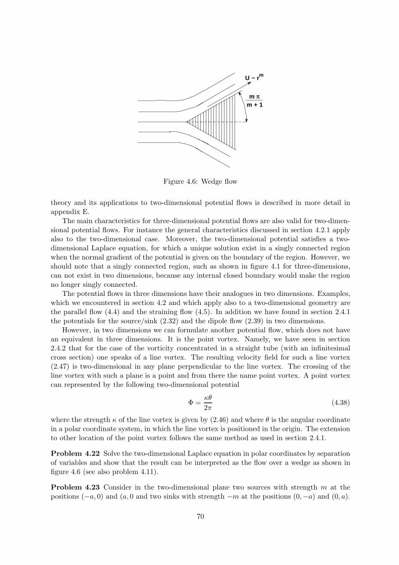
m πm + 1

U ~ rm

Figure 4.6: Wedge flow

theory and its applications to two-dimensional potential flows is described in more detail inappendix E.

The main characteristics for three-dimensional potential flows are also valid for two-dimen-sional potential flows. For instance the general characteristics discussed in section 4.2.1 applyalso to the two-dimensional case. Moreover, the two-dimensional potential satisfies a two-dimensional Laplace equation, for which a unique solution exist in a singly connected regionwhen the normal gradient of the potential is given on the boundary of the region. However, weshould note that a singly connected region, such as shown in figure 4.1 for three-dimensions,can not exist in two dimensions, because any internal closed boundary would make the regionno longer singly connected.

The potential flows in three dimensions have their analogues in two dimensions. Examples,which we encountered in section 4.2 and which apply also to a two-dimensional geometry arethe parallel flow (4.4) and the straining flow (4.5). In addition we have found in section 2.4.1the potentials for the source/sink (2.32) and the dipole flow (2.39) in two dimensions.

However, in two dimensions we can formulate another potential flow, which does not havean equivalent in three dimensions. It is the point vortex. Namely, we have seen in section2.4.2 that for the case of the vorticity concentrated in a straight tube (with an infinitesimalcross section) one speaks of a line vortex. The resulting velocity field for such a line vortex(2.47) is two-dimensional in any plane perpendicular to the line vortex. The crossing of theline vortex with such a plane is a point and from there the name point vortex. A point vortexcan represented by the following two-dimensional potential

Φ =κθ

2π(4.38)

where the strength κ of the line vortex is given by (2.46) and where θ is the angular coordinatein a polar coordinate system, in which the line vortex is positioned in the origin. The extensionto other location of the point vortex follows the same method as used in section 2.4.1.

Problem 4.22 Solve the two-dimensional Laplace equation in polar coordinates by separationof variables and show that the result can be interpreted as the flow over a wedge as shown infigure 4.6 (see also problem 4.11).

Problem 4.23 Consider in the two-dimensional plane two sources with strength m at thepositions (−a, 0) and (a, 0 and two sinks with strength −m at the positions (0,−a) and (0, a).

70

Compute the stream function and draw the streamline pattern. Show that there is a closedstreamline and compute the velocity and pressure on this closed streamline.

Problem 4.24 Consider the two-dimensional flow given by the potential

Φ = −Uy[1 +

1x2 + y2

+2

(x+ 1)2 + y2+

2(x− 1)2 + y2

].

Compute the stream function and show that this flow describes the flow around a solid body.Find this body and compute the velocity and pressure on the body.

Problem 4.25 Consider in the two-dimensional plane two sources with strength m at the po-sitions (−a, 0) and (a, 0) and a sink with strength −2m at the origin. Show that the streamlinesare curves given by (

x2 + y2)2 = a2

(x2 − y2 + λxy

).

Compare this result with problem 2.10.

Problem 4.26 Redo problem 4.14 but now with the potential (2.10) in a straining flow

u = −αx, v = αy

with α a positive constant. Compute the potential and the stream function. Show that theresult describes the flow around a closed body. Determine the shape of the body and calculatethe velocity and pressure on the surface of this body.

Problem 4.27 Consider the conformal transformation

ζ = zn

and show that with help of this transformation we can compute the flow in a wedge with angleα = π/n.

Problem 4.28 Consider the conformal transformation of the ζ- to the z-plane according toζ = z2. Show that the half-plane (ζ) > 0 transforms to the 1st quadrant in the z-plane.Next consider a free point vortex in the ζ-plane and with strength κ at the position ζ = δ2

with δ = δx + i δy near a fixed wall in the ζ-plane along the real axis. Compute and interpretthe resulting flow in the z-plane. Determine the trajectory, which the vortex describes in thez-plane.

Problem 4.29 Consider the conformal transformation of the ζ- to the z-plane according toζ = z1/2. Show that the line ζ = ξ + i δ with δ a real constant > 0 transforms into a parabolain the z-plane. Next consider a free point vortex at the position ζ0 = (ζ0) + i(ζ0) in theζ-plane with (ζ0) > δ. The vortex moves with a velocity U parallel to the real axis in theζ-plane. Compute the trajectory, which the vortex describes in the z-plane and determine theforce on the parabola as a function of time.

71

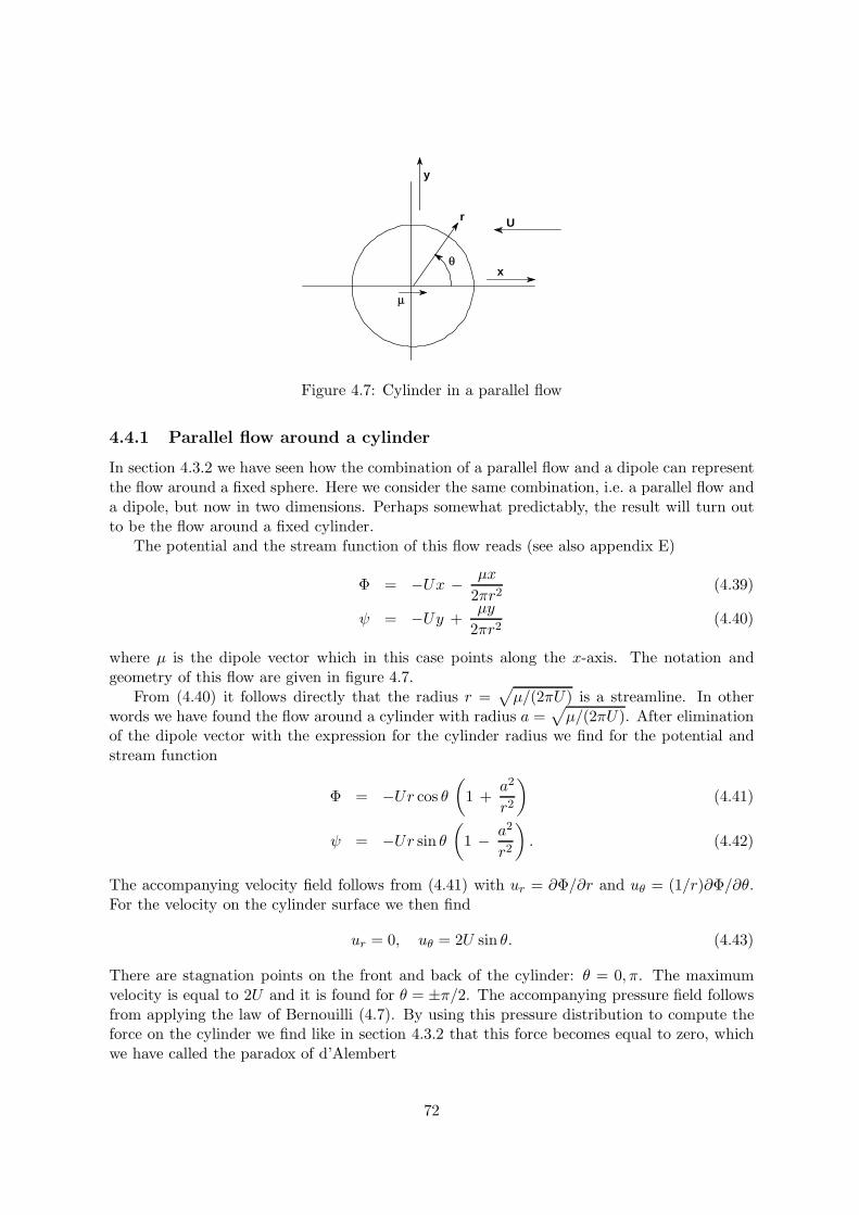
U

x

y

r

µ

θ

Figure 4.7: Cylinder in a parallel flow

4.4.1 Parallel flow around a cylinder

In section 4.3.2 we have seen how the combination of a parallel flow and a dipole can representthe flow around a fixed sphere. Here we consider the same combination, i.e. a parallel flow anda dipole, but now in two dimensions. Perhaps somewhat predictably, the result will turn outto be the flow around a fixed cylinder.

The potential and the stream function of this flow reads (see also appendix E)

Φ = −Ux − µx

2πr2(4.39)

ψ = −Uy +µy

2πr2(4.40)

where µ is the dipole vector which in this case points along the x-axis. The notation andgeometry of this flow are given in figure 4.7.

From (4.40) it follows directly that the radius r =√µ/(2πU) is a streamline. In other

words we have found the flow around a cylinder with radius a =√µ/(2πU). After elimination

of the dipole vector with the expression for the cylinder radius we find for the potential andstream function

Φ = −Ur cos θ(

1 +a2

r2

)(4.41)

ψ = −Ur sin θ(

1 − a2

r2

). (4.42)

The accompanying velocity field follows from (4.41) with ur = ∂Φ/∂r and uθ = (1/r)∂Φ/∂θ.For the velocity on the cylinder surface we then find

ur = 0, uθ = 2U sin θ. (4.43)

There are stagnation points on the front and back of the cylinder: θ = 0, π. The maximumvelocity is equal to 2U and it is found for θ = ±π/2. The accompanying pressure field followsfrom applying the law of Bernouilli (4.7). By using this pressure distribution to compute theforce on the cylinder we find like in section 4.3.2 that this force becomes equal to zero, whichwe have called the paradox of d’Alembert

72

θ Ω t − Ω t

r

Figure 4.8: Geometry of two moving walls.

Analogous to the procedure that we have applied in section 4.3.3 we can compute the flowaround a cylinder which moves with a velocity U in an infinite non-moving, non-viscous fluid.In this case the contribution of the parallel flow must subtracted from (4.41) and 4.42, so thatonly the dipole contribution remains.

Again we can compute the kinetic energy of this flow (note that in this case we have tocompute in the two-dimensional x− y plane outside of the cylinder). Without details we givehere the answer, which reads

T =12ρπa2U2. (4.44)

From this result it follows that the virtual or added mass of a cylinder is equal to

Mv = ρπa2. (4.45)

This means that the Mv in this case is equal to the displaced mass of fluid and it is thus largerthat the value (4.33), which we have found for the sphere.

Problem 4.30 A cylinder with radius a in a non-viscous fluid with density ρ carries out smalloscillations given by U = U0 sinωt. Compute the force per unit length on the cylinder. Thedensity of the cylinder material is ρc.

Problem 4.31 The space between two coaxial cylindrical shells of radii a and b is filled witha non-viscous liquid with density ρ. The outer shell with radius a is suddenly made to movewith velocity U . Show that the impulsive force (per unit length) applied on the inner cylinderis given by

F =2πρa2b2U

a2 − b2.

Problem 4.32 Two rigid walls rotate with an angular speed Ωt and −Ωt. In the spacebetween the walls: 0 < r <∞ and −Ωt < θ < Ωt (as illustrated in figure 4.8) is a non-viscousfluid . The flow can be described by a two-dimensional potential flow. Use the methodsof separation of variables, i.e. Φ = R(r)Θ(θ) to find a solution for the Laplace equation (incylinder coordinates). Compute the stream function and the pressure on the walls. Show thatthe solution breaks down when the angle between the walls approaches the value π.

Problem 4.33 Consider the Joukowski transformation from the ζ- to the z-plane given by

z = ζ − ζ

λ2.

Show that a circle in the ζ-plane with radius λ transforms to a flat plate with width 4λ alongthe y-axis in the z-plane. Furthermore show that a circle in the ζ-plane with radius a > λtransforms to an ellipse with its minor-axis along the x-axis in the z-plane. Consider only theparts of the flat plate and ellipse above the x-axis. Use these results to compute the flow aroundthese half-bodies in an oncoming parallel flow with velocity U along the x-axis. Compute theforce on both half-bodies.

73

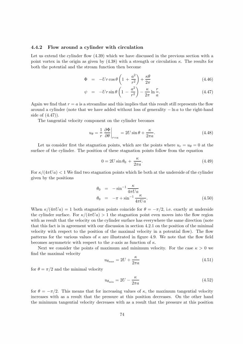
4.4.2 Flow around a cylinder with circulation

Let us extend the cylinder flow (4.39) which we have discussed in the previous section with apoint vortex in the origin as given by (4.38) with a strength or circulation κ. The results forboth the potential and the stream function then become

Φ = −Ur cos θ(

1 +a2

r2

)+κθ

2π(4.46)

ψ = −Ur sin θ(

1 − a2

r2

)− κ

2πlnr

a. (4.47)

Again we find that r = a is a streamline and this implies that this result still represents the flowaround a cylinder (note that we have added without loss of generality − ln a to the right-handside of (4.47)).

The tangential velocity component on the cylinder becomes

uθ =1r

∂Φ∂θ

∣∣∣∣r=a

= 2U sin θ +κ

2πa. (4.48)

Let us consider first the stagnation points, which are the points where ur = uθ = 0 at thesurface of the cylinder. The position of these stagnation points follow from the equation

0 = 2U sin θ0 +κ

2πa. (4.49)

For κ/(4πUa) < 1 We find two stagnation points which lie both at the underside of the cylindergiven by the positions

θ0 = − sin−1 κ

4πUaθ0 = −π + sin−1 κ

4πUa. (4.50)

When κ/(4πUa) = 1 both stagnation points coincide for θ = −π/2, i.e. exactly at undersidethe cylinder surface. For κ/(4πUa) > 1 the stagnation point even moves into the flow regionwith as result that the velocity on the cylinder surface has everywhere the same direction (notethat this fact is in agreement with our discussion in section 4.2.1 on the position of the minimalvelocity with respect to the position of the maximal velocity in a potential flow). The flowpatterns for the various values of κ are illustrated in figure 4.9. We note that the flow fieldbecomes asymmetric with respect to the x-axis as function of κ.

Next we consider the points of maximum and minimum velocity. For the case κ > 0 wefind the maximal velocity

uθmax = 2U +κ

2πa(4.51)

for θ = π/2 and the minimal velocity

uθmin= 2U − κ

2πa(4.52)

for θ = −π/2. This means that for increasing values of κ, the maximum tangential velocityincreases with as a result that the pressure at this position decreases. On the other handthe minimum tangential velocity decreases with as a result that the pressure at this position

74

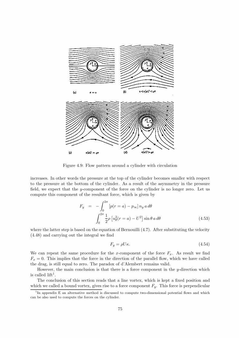
Figure 4.9: Flow pattern around a cylinder with circulation

increases. In other words the pressure at the top of the cylinder becomes smaller with respectto the pressure at the bottom of the cylinder. As a result of the asymmetry in the pressurefield, we expect that the y-component of the force on the cylinder is no longer zero. Let uscompute this component of the resultant force, which is given by

Fy = −∫ 2π

0[p(r = a) − p∞]ny a dθ∫ 2π

0

12ρ[u2

θ(r = a) − U2]sin θ a dθ (4.53)

where the latter step is based on the equation of Bernouilli (4.7). After substituting the velocity(4.48) and carrying out the integral we find

Fy = ρUκ. (4.54)

We can repeat the same procedure for the x-component of the force Fx. As result we findFx = 0. This implies that the force in the direction of the parallel flow, which we have calledthe drag, is still equal to zero. The paradox of d’Alembert remains valid.

However, the main conclusion is that there is a force component in the y-direction whichis called lift1.

The conclusion of this section reads that a line vortex, which is kept a fixed position andwhich we called a bound vortex, gives rise to a force component Fy. This force is perpendicular

1In appendix E an alternative method is discussed to compute two-dimensional potential flows and whichcan be also used to compute the forces on the cylinder.

75

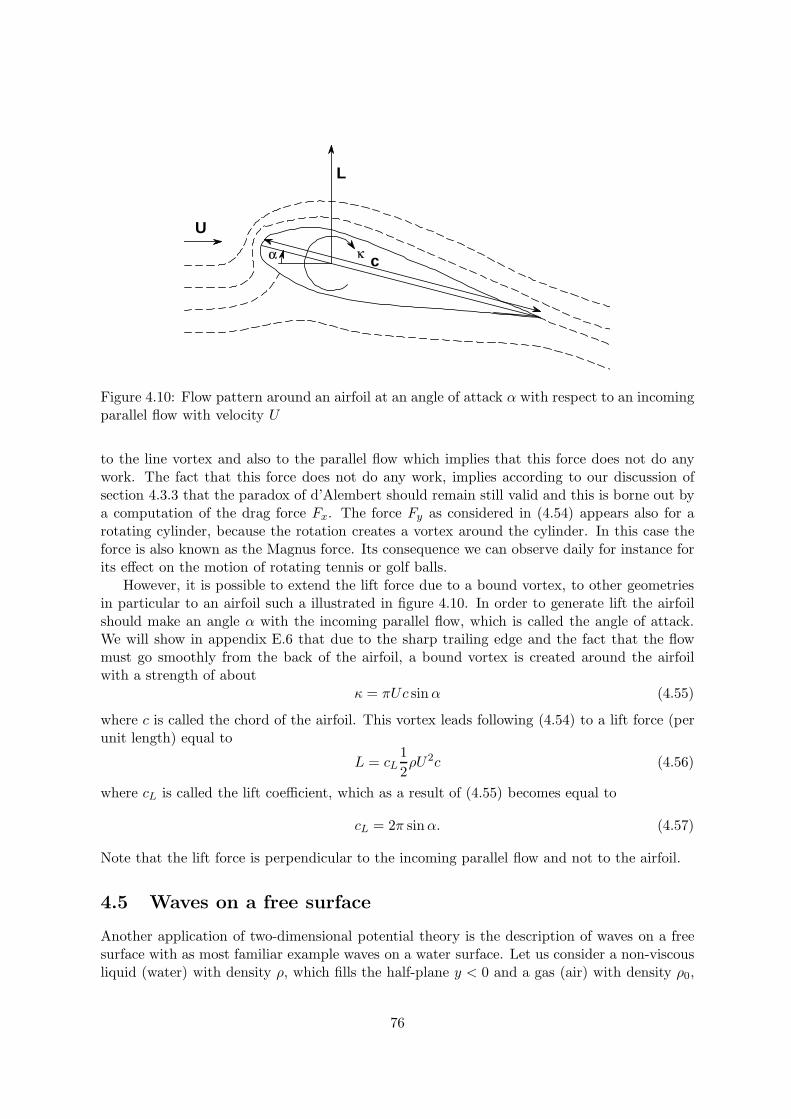
L

U

α κ c

Figure 4.10: Flow pattern around an airfoil at an angle of attack α with respect to an incomingparallel flow with velocity U

to the line vortex and also to the parallel flow which implies that this force does not do anywork. The fact that this force does not do any work, implies according to our discussion ofsection 4.3.3 that the paradox of d’Alembert should remain still valid and this is borne out bya computation of the drag force Fx. The force Fy as considered in (4.54) appears also for arotating cylinder, because the rotation creates a vortex around the cylinder. In this case theforce is also known as the Magnus force. Its consequence we can observe daily for instance forits effect on the motion of rotating tennis or golf balls.

However, it is possible to extend the lift force due to a bound vortex, to other geometriesin particular to an airfoil such a illustrated in figure 4.10. In order to generate lift the airfoilshould make an angle α with the incoming parallel flow, which is called the angle of attack.We will show in appendix E.6 that due to the sharp trailing edge and the fact that the flowmust go smoothly from the back of the airfoil, a bound vortex is created around the airfoilwith a strength of about

κ = πUc sinα (4.55)

where c is called the chord of the airfoil. This vortex leads following (4.54) to a lift force (perunit length) equal to

L = cL12ρU2c (4.56)

where cL is called the lift coefficient, which as a result of (4.55) becomes equal to

cL = 2π sinα. (4.57)

Note that the lift force is perpendicular to the incoming parallel flow and not to the airfoil.

4.5 Waves on a free surface

Another application of two-dimensional potential theory is the description of waves on a freesurface with as most familiar example waves on a water surface. Let us consider a non-viscousliquid (water) with density ρ, which fills the half-plane y < 0 and a gas (air) with density ρ0,

76

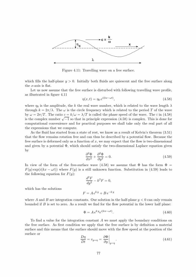
λ

η x0

c =kω

Figure 4.11: Travelling wave on a free surface.

which fills the half-plane y > 0. Initially both fluids are quiescent and the free surface alongthe x-axis is flat.

Let us now assume that the free surface is disturbed with following travelling wave profile,as illustrated in figure 4.11

η(x, t) = η0 ei(kx−ωt), (4.58)

where η0 is the amplitude, the k the real wave number, which is related to the wave length λthrough k = 2π/λ. The ω is the circle frequency which is related to the period T of the waveby ω = 2π/T . The ratio c = k/ω = λ/T is called the phase speed of the wave. The i in (4.58)is the complex number

√−1 so that in principle expression (4.58) is complex. This is done forcomputational convenience and for practical purposes we shall take only the real part of allthe expressions that we compute.

As the fluid has started from a state of rest, we know as a result of Kelvin’s theorem (3.51)that the flow remains rotation free and can thus be described by a potential flow. Because thefree surface is deformed only as a function of x, we may expect that the flow is two-dimensionaland given by a potential Φ, which should satisfy the two-dimensional Laplace equation givenby

∂2Φ∂x2

+∂2Φ∂y2

= 0. (4.59)

In view of the form of the free-surface wave (4.58) we assume that Φ has the form Φ =F (y) exp(i(kx − ωt)) where F (y) is a still unknown function. Substitution in (4.59) leads tothe following equation for F (y):

d2F

dy2− k2F = 0,

which has the solutionsF = Aek y +B e−k y

where A and B are integration constants. Our solution in the half-plane y < 0 can only remainbounded if B is set to zero. As a result we find for the flow potential in the lower half plane:

Φ = Aek yei(kx−ωt). (4.60)

To find a value for the integration constant A we must apply the boundary conditions onthe free surface. As first condition we apply that the free surface is by definition a materialsurface and this means that the surface should move with the flow speed at the position of thesurface or

Dη

Dt= vy=η =

∂Φ∂y

∣∣∣∣y=η

. (4.61)

77

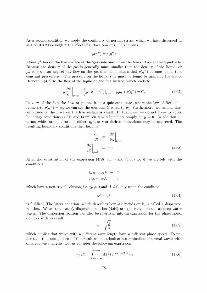
As a second condition we apply the continuity of normal stress, which we have discussed insection 3.3.2 (we neglect the effect of surface tension). This implies

p(η+) = p(η−)

where η+ lies on the free surface at the ‘gas’-side and η− on the free surface at the liquid side.Because the density of the gas is generally much smaller than the density of the liquid, orρ0 ρ we can neglect any flow on the gas side. This means that p(η+) becomes equal to aconstant pressure p0. The pressure on the liquid side must be found by applying the law ofBernouilli (4.7) to the flow of the liquid on the free surface, which leads to

ρ∂Φ∂t

∣∣∣∣y=η

+12ρ(u2 + v2

)∣∣y=η

+ ρgη + p(η−) = C. (4.62)

In view of the fact the flow originates from a quiescent state, where the law of Bernouillireduces to p(η−) = p0, we can set the constant C equal to p0. Furthermore, we assume thatamplitude of the wave on the free surface is small. In that case we do not have to applyboundary conditions (4.61) and (4.62) on y = η but more simply on y = 0. In addition allterms, which are quadratic in either, η, u or v or their combinations, may be neglected. Theresulting boundary conditions then become

∂η

∂t=

∂Φ∂y

∣∣∣∣y=0

∂Φ∂t

∣∣∣∣y=0

= gη. (4.63)

After the substitution of the expression (4.58) for η and (4.60) for Φ we are left with theconditions

iω η0 −Ak = 0g η0 + i ωA = 0,

which have a non-trivial solution, i.e. η0 = 0 and A = 0 only when the condition

ω2 = gk (4.64)

is fulfilled. The latter equation, which describes how ω depends on k, is called a dispersionrelation. Waves that satisfy dispersion relation (4.64) are generally denoted as deep waterwaves. The dispersion relation can also be rewritten into an expression for the phase speedc = ω/k with as result

c =√g

k(4.65)

which implies that waves with a different wave length have a different phase speed. To un-derstand the consequences of this result we must look at a combination of several waves withdifferent wave lengths. Let us consider the following expression

η (x, t) =∫ k=∞

k=−∞A (k) ei[kx−ω(k)t] dk (4.66)

78

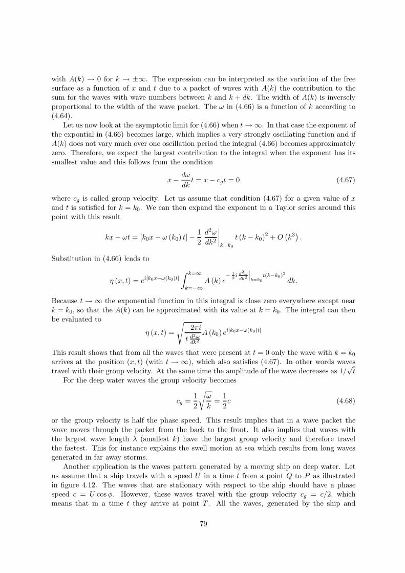
with A(k) → 0 for k → ±∞. The expression can be interpreted as the variation of the freesurface as a function of x and t due to a packet of waves with A(k) the contribution to thesum for the waves with wave numbers between k and k + dk. The width of A(k) is inverselyproportional to the width of the wave packet. The ω in (4.66) is a function of k according to(4.64).

Let us now look at the asymptotic limit for (4.66) when t→ ∞. In that case the exponent ofthe expontial in (4.66) becomes large, which implies a very strongly oscillating function and ifA(k) does not vary much over one oscillation period the integral (4.66) becomes approximatelyzero. Therefore, we expect the largest contribution to the integral when the exponent has itssmallest value and this follows from the condition

x− dω

dkt = x− cgt = 0 (4.67)

where cg is called group velocity. Let us assume that condition (4.67) for a given value of xand t is satisfied for k = k0. We can then expand the exponent in a Taylor series around thispoint with this result

kx− ωt = [k0x− ω (k0) t] − 12d2ω

dk2

∣∣∣∣k=k0

t (k − k0)2 +O

(k3).

Substitution in (4.66) leads to

η (x, t) = ei[k0x−ω(k0)t]

∫ k=∞

k=−∞A (k) e

− 12i d2ω

dk2

∣∣∣k=k0

t(k−k0)2

dk.

Because t → ∞ the exponential function in this integral is close zero everywhere except neark = k0, so that the A(k) can be approximated with its value at k = k0. The integral can thenbe evaluated to

η (x, t) =

√−2πi

t d2ωdk2

A (k0) ei[k0x−ω(k0)t]

This result shows that from all the waves that were present at t = 0 only the wave with k = k0

arrives at the position (x, t) (with t → ∞), which also satisfies (4.67). In other words wavestravel with their group velocity. At the same time the amplitude of the wave decreases as 1/

√t

For the deep water waves the group velocity becomes

cg =12

√ω

k=

12c (4.68)

or the group velocity is half the phase speed. This result implies that in a wave packet thewave moves through the packet from the back to the front. It also implies that waves withthe largest wave length λ (smallest k) have the largest group velocity and therefore travelthe fastest. This for instance explains the swell motion at sea which results from long wavesgenerated in far away storms.

Another application is the waves pattern generated by a moving ship on deep water. Letus assume that a ship travels with a speed U in a time t from a point Q to P as illustratedin figure 4.12. The waves that are stationary with respect to the ship should have a phasespeed c = U cosφ. However, these waves travel with the group velocity cg = c/2, whichmeans that in a time t they arrive at point T . All the waves, generated by the ship and

79

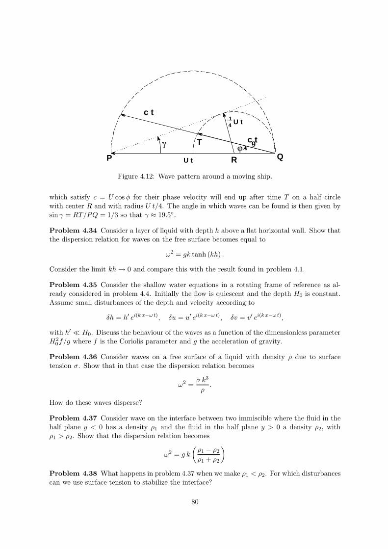
c t

c tg

U t

14 U t

γQP

ϕT

R

Figure 4.12: Wave pattern around a moving ship.

which satisfy c = U cosφ for their phase velocity will end up after time T on a half circlewith center R and with radius U t/4. The angle in which waves can be found is then given bysin γ = RT/PQ = 1/3 so that γ ≈ 19.5.

Problem 4.34 Consider a layer of liquid with depth h above a flat horizontal wall. Show thatthe dispersion relation for waves on the free surface becomes equal to

ω2 = gk tanh (kh) .

Consider the limit kh→ 0 and compare this with the result found in problem 4.1.

Problem 4.35 Consider the shallow water equations in a rotating frame of reference as al-ready considered in problem 4.4. Initially the flow is quiescent and the depth H0 is constant.Assume small disturbances of the depth and velocity according to

δh = h′ ei(k x−ω t), δu = u′ ei(k x−ω t), δv = v′ ei(k x−ω t),

with h′ H0. Discuss the behaviour of the waves as a function of the dimensionless parameterH2

0f/g where f is the Coriolis parameter and g the acceleration of gravity.

Problem 4.36 Consider waves on a free surface of a liquid with density ρ due to surfacetension σ. Show that in that case the dispersion relation becomes

ω2 =σ k3

ρ.

How do these waves disperse?

Problem 4.37 Consider wave on the interface between two immiscible where the fluid in thehalf plane y < 0 has a density ρ1 and the fluid in the half plane y > 0 a density ρ2, withρ1 > ρ2. Show that the dispersion relation becomes

ω2 = g k

(ρ1 − ρ2

ρ1 + ρ2

)

Problem 4.38 What happens in problem 4.37 when we make ρ1 < ρ2. For which disturbancescan we use surface tension to stabilize the interface?

80

Problem 4.39 A layer of non-viscous fluid flows with velocity U over a corrugated bed givenby y = −H0 + ε cos k x where H0 is the average depth of the layer and where ε H0 (theorigin of the coordinate system lies at the average free surface). Find the disturbances of thefree surface as function of the parameter U2/(gH0).

Problem 4.40 Consider the shallow water equations in a rotation frame of reference (seeproblems 4.1 and 4.4). The starting point is no motion and a constant depth H0. We perturbthis situation with a small variation only in the velocity components. Derive by linearisingthe equations that an oscillating solution is possible with period 2π/f where f is the Coriolisparameter. These are known as inertial oscillations. Next introduce also small perturbationsin the depth. Consider the linearized equations and discuss the relevance of the velocity fH0.

Problem 4.41 Consider the shallow water equations in a rotation frame of reference (seeproblems 4.1 and 4.4) in the so-called β-plane approximation, i.e. the Coriolis parameter isgiven by f = f0 +β y (β > 0). The starting point is a flow with a constant velocity U = (U, 0),i.e. with only a component along the positive x-axis and with a constant depth H0. Perturbthis flow with small velocity perturbations (the depth remains constant). Derive the dispersionrelation of the resulting waves, which are known as Rossby waves. Next allow also perturbationsin the depth and discuss the role of the Rossby number U/(f0H0) and the Rossby radius ofdeformation Rb =

√gH0/f0 for the cases β = 0 and β =/ 0.

81

Chapter 5

Thermodynamics

5.1 Conservation of energy

We have seen in the previous chapter that potential flows have many important applications,such as the theory of lift, surface waves etc. Nevertheless from a physical point of viewpotential flow exhibits an important flaw, which has been illustrated by means of the paradoxof d’Alembert. Namely, it requires no energy to maintain a stationary potential flow.

In section 4.3.3 we have related the paradox of d’Alembert to the lack of loss processes. Thisfollows in the first place from the fact that potential flow is a solution of the Euler equationsor alternatively the equations of motion for an ideal fluid. Viscous shear stresses are in such afluid by definition equal to zero. We must therefore conclude that with help of an ideal fluidwe can not describe all aspects of a realistic flow problem and this is in particular the casewith respect to the drag.

The key word is ideal fluid, because we have stated in section 4.1 that a potential flow is alsothe solution of the complete equations of motion (3.37), i.e. including the viscous terms. Thiswould seem to imply a paradox. However, we have also stressed that a potential flow, takenas solution of the Navier-Stokes equations, in general does not satisfy the no-slip condition. Inother words this boundary condition (or more general the existence of shear stress on a wall)is the basis of drag and we shall come back to this in more detail in chapter 6.

Let us return to the complete equations of motion (3.37). Before we derive the solutionsof this set of equation, we shall first consider the effect of viscosity in general terms. This weshall do by introducing a new equation, which describes the conservation of energy.

Our point of departure is again a material fluid element with volume δV and mass δM ,which by definition follows all flow motions, so no transport takes place through the wall ofthe fluid element. This means that such a fluid elements can be considered as closed system.To such a closed system we can apply the first law of thermodynamics, which per unit massreads

∆Etot = Q+W (5.1)

where ∆Etot is the change of the total energy of the fluid element; Q is the amount of heatadded to the element and W the work exerted on the element (sometimes we take the workperformed by the element and in that case we should write −W in (5.1)).

The total energy is equal to

Etot = E +12u2 (5.2)

82

where E is the internal energy and 1/2u2 the kinetic energy of the flow field, both per unitmass. In order to express the internal energy in other variables we shall make use of theclassical equilibrium thermodynamics. This implies that we assume that the fluid elementis always in thermodynamical equilibrium. It will be clear that a flow by definition can notbe in equilibrium, i.e. the flow itself is a non-equilibrium process. However, the deviationsof equilibrium for each fluid element will be negligible if the time scale of the flow is muchlarger than the molecular time scale, by which equilibrium establishes itself. This is for mostpractical flows the case. (See for instance problem 1.2.)

For a thermodynamic system in equilibrium the E is a so-called state variable. Equilibriumthermodynamics states that a homogeneous system, can be described completely in terms ofjust two state variables. Homogeneous in this case means that a system has everywhere thesame constant composition. So we do not take into account phase changes or chemical species,which may react into new components. For the base state variables we choose the densityρ and the absolute temperature T . (On the side we note that the extrapolation of thesethermodynamical state variable to a situation of non-equilibrium, like a flowing medium, notalways trivial. This is in particular the case for the temperature and for a more detaileddiscussion we refer to the section 3.4 of the book of Batchelor.)

For the internal energy of a flowing medium which satisfies the restrictions mentioned abovewith respect to equilibrium, it now follows

E = f(ρ, T ). (5.3)

This equation is know as the caloric equation. For an ideal gas we have

E = cvT (5.4)

where cv is the specific heat at constant volume.Next we introduce the thermodynamical equation of state, which describes a relationship

between the thermodynamical state variables in the following form

pe = f(ρ, T ) (5.5)

where pe is called the thermodynamical pressure. For an ideal gas we have

pe = RρT. (5.6)

In principle the pe is not equal to the mechanical pressure, which we have defined as themean of the normal stress in the three coordinate directions in section 3.2.2. Only whenequilibrium applies exactly, i.e. in a fluid with no motion, we can state pe = p ≡ −1

3σkk.However, based on the hypothesis mentioned above that deviations of equilibrium are small,we shall also use in a flowing medium

pe = −13σkk. (5.7)

This means that we can express the pressure, which appears in the equations of motion (3.37),with help of (5.5) in terms of the other state variables, ρ en T .

Let us now return to the first law of thermodynamics for a material fluid element (5.1).Based on this we compute the change of energy of a material volume V with a surface A anda outside normal n. Using (3.5) we find∫ ∫ ∫

VρDEtot

DtdV =

∫ ∫ ∫Vρfiui dV +

∫ ∫Aσijui nj dS +

∫ ∫Ak∂T

∂xini dS. (5.8)

83

The first two terms on the right-hand side of (5.8) represent the work, which is performed bythe volume or body forces and surface stresses. The third term in (5.8) is the heat, which issupplied to the volume by molecular conduction where k is called the conductivity.

With help of the divergence theorem (A.10) we can convert the surface integrals in (5.8) intovolume integrals. Moreover, the resulting expression must be valid for any arbitrary volumeV , so that we can equate the integrand on the left and right-hand side with as result

ρDEtot

Dt= ρfiui +

∂uiσij

∂xj+

∂

∂xi

(k∂T

∂xi

). (5.9)

With help of (5.2) and (3.17) it then follows that

ρDE

Dt= σij

∂ui

∂xj+

∂

∂xi

(k∂T

∂xi

). (5.10)

This equation gives the general expression in differential form of the conservation of internalenergy in a flow.

Next we substitute in (5.10) the constitutive relation (3.35) for a Newtonian fluid with asresult

ρDE

Dt= −p∆ + 2µ

(eij − 1

3∆δij

)∂ui

∂xj+

∂

∂xi

(k∂T

∂xi

)

= −p∆ + 2µ(e2ij −

13∆2

)+

∂

∂xi

(k∂T

∂xi

)

= −p∆ + 2µ(eij − 1

3∆δij

)2

+∂

∂xi

(k∂T

∂xi

)(5.11)

where we have used for the last step the identity (eij − 13∆δij)2 = e2ij − 2

3eij∆δij + 19∆2δij2,

which with δ2ij = δii = 3 and δijeij = ∆ goes over in e2ij − 13∆2.

The first term on the right-hand side of (5.11) is the work, which is performed by theisotropic part of the stress tensor. We have mentioned before that this part gives the expan-sion/compression in the flow. In other words this terms represents the reversible work throughchange of volume

The second term is the work done by the deviatoric stresses which is also called the defor-mation work. We find that this deformation work is always positive! The background is thatin a real fluid, i.e. µ =/ 0, kinetic energy is converted constantly in internal energy (heat). Thisis the loss process, which we have mentioned in the beginning of this chapter. Therefore, thisterm is denoted as the dissipation.

The third term in the equation gives the change of internal energy as a result of thetransport of heat into the volume due to molecular conduction.

We can conclude from (5.11), that in a real fluid there will be always a loss process relatedto dissipation. Therefore, in order to maintain even a stationary flow we must continuouslyperform work. This work can be interpreted as the drag which a body experiences in a flowof a real fluid. This is the fundamental difference with the flow of an ideal fluid flow, in whichthere are no loss processes as discussed in section 4.3.3.

84

5.2 Entropy

The effect of viscous dissipation can be made also visible with help of the first law of thermo-dynamics in another form. This reads

TDS

Dt=DE

Dt+ p

D

Dt

(1ρ

)(5.12)

where S is the entropy. The entropy is a state variable, which measures the amount of disorderin a system. Because (5.12) contains only state variables, we can consider it as the definitionof entropy.

With help of the continuity equation (2.3) it follows that D(1/ρ)/Dt = ∆/ρ. After substi-tution in (5.12) and after use of (5.11) we find

TDS

Dt= 2

µ

ρ

(eij − 1

3∆δij

)2

+1ρ

∂

∂xi

(k∂T

∂xi

). (5.13)

From this equation it follows that, if we for the moment neglect heat conduction, dissipationgoes together with an increase of entropy or an increase of the disorder of a system. In otherwords, useful mechanical energy, which has the form of the kinetic energy of the ordered motionof the flow, is transformed by means of dissipation in disordered molecular motions, which wecall heat.

At the same time it follows from (5.13) that for a ideal fluid, i.e. µ = 0 and k = 0, theenergy equation can be written in compact form as

DS

Dt= 0. (5.14)

This implies that for an ideal fluid entropy is a material quantity, which stays constant alongthe path of a fluid elements. The process, for which (5.14) applies is also called an isentropicprocess.

5.3 Energy integral

It is often useful to formulate the conservation of energy in terms of a so-called energy integral.The point of departure is (5.9) for an incompressible flow and a Newtonian fluid. It thenfollows

D

Dt

(E +

12u2

i

)= uifi − 1

ρ

∂uip

∂xi+

1ρ

∂

∂xj

[2µui

(eij − 1

3∆δij

)]+

1ρ

∂

∂xi

(k∂T

∂xi

). (5.15)

Let us now make the following assumptions:

1. The volume forces (fi) are conservative.So there is a force potential, Ψ, which satisfies

fi = − ∂Ψ∂xi

. (5.16)

It then followsuifi = −ui

∂Ψ∂xi

= −DΨDt

(5.17)

85

because ∂Ψ/∂t ≡ 0.

2. The flow is stationary.This means that p =/ p(t), so that

−1ρ

∂uip

∂xi= −p

ρ

∂ui

∂xi− ui

ρ

∂p

∂xi

=p

ρ2

Dρ

Dt− 1ρ

Dp

Dt(5.18)

= −DDt

(p

ρ

).

Substitution of (5.17) and (5.18) in (5.15) then leads to the following expression

DH

Dt=

1ρ

∂

∂xj

[2µui

(eij − 1

3∆δij

)+ k

∂T

∂xj

](5.19)

where the variable H is equal to

H = E +12u2

i +p

ρ+ Ψ. (5.20)

We can thus attribute to a fluid element a variable H, which varies along the trajectory ofthe fluid element only as a result of friction or heat conduction. For an ideal fluid where µ = 0en k = 0, we can integrate (5.19) directly with as result

H = constant (5.21)

along the trajectory of the fluid element. Because we consider a stationary flow, the trajectoryis also equal to a streamline. The result (5.21) is known as the general form of the law ofBernouilli.

In terms of classical mechanics we can interpret (5.21) as T + V = constant, where T =E+ 1

2u2i is the total kinetic energy, i.e. the sum of the molecular and macroscopic kinetic energy,

and V = p/ρ + Ψ as the potential energy (although the pressure is in principle somethingdifferent than potential energy). For this reason (5.21) is also called the energy integral.

For the special case of an incompressible flow, to which we have restricted ourselves up tonow, we can simplify (5.20) even further. We have argued that the internal energy is a functionof two state variables. Let us choose S en ρ for these variables. It then follows

DE

Dt=(∂E

∂ρ

)S

Dρ

Dt+(∂E

∂S

)ρ

DS

Dt. (5.22)

As we have seen in section 2.1 the condition for incompressible flow is Dρ/Dt = 0, whereasfor an ideal fluid the energy equation reduces to DS/Dt = 0 (5.14). With help of (5.22) thisthen leads to the result that E is constant along the path of a fluid element. Therefore, wecan incorporate the E in the integration constant. With this we find

H =12u2

i +p

ρ+ Ψ = constant. (5.23)

Note that this expression, although similar to the law of Bernouilli for the potential flow (4.7)applies to quite different conditions. To repeat these conditions they are: stationary flow, an

86

ideal fluid, i.e. no viscosity of heat conduction, conservative body force and most important His constant along a stream line but may vary from streamline to streamline.

We mentioned above that the variableH is only constant along a stream line and in principlecan vary from one streamline to another. However, with the help of Crocco’s theorem, we candetermine how H varies as a function of the spatial coordinates. This theorem reads

∇H = T ∇S + u× ω (5.24)

and it is proved in appendix F. It shows that for constant entropy H is constant when ω = 0,which is the condition that we encountered in the case of potential flow. However, (5.24) showsthat H can be also constant in the special case when u aligns everywhere with ω. This lattercondition is satisfied for a special class of flows, which are known as Beltrami flows. Finally,we see that a constant H also requires a constant entropy and this type of flow is known ashomentropic.

87

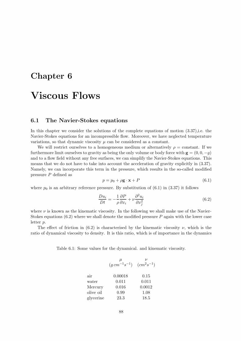
Chapter 6

Viscous Flows

6.1 The Navier-Stokes equations

In this chapter we consider the solutions of the complete equations of motion (3.37),i.e. theNavier-Stokes equations for an incompressible flow. Moreover, we have neglected temperaturevariations, so that dynamic viscosity µ can be considered as a constant.

We will restrict ourselves to a homogeneous medium or alternatively ρ = constant. If wefurthermore limit ourselves to gravity as being the only volume or body force with g = (0, 0,−g)and to a flow field without any free surfaces, we can simplify the Navier-Stokes equations. Thismeans that we do not have to take into account the acceleration of gravity explicitly in (3.37).Namely, we can incorporate this term in the pressure, which results in the so-called modifiedpressure P defined as

p = p0 + ρg · x + P (6.1)

where p0 is an arbitrary reference pressure. By substitution of (6.1) in (3.37) it follows

Dui

Dt= −1

ρ

∂P

∂xi+ ν

∂2ui

∂x2j

(6.2)

where ν is known as the kinematic viscosity. In the following we shall make use of the Navier-Stokes equations (6.2) where we shall denote the modified pressure P again with the lower caseletter p.

The effect of friction in (6.2) is characterised by the kinematic viscosity ν, which is theratio of dynamical viscosity to density. It is this ratio, which is of importance in the dynamics

Table 6.1: Some values for the dynamical. and kinematic viscosity.

µ ν(g cm−1s−1) (cm2s−1)

air 0.00018 0.15water 0.011 0.011Mercury 0.016 0.0012olive oil 0.99 1.08glycerine 23.3 18.5

88

because the viscous stresses must be able to accelerate fluid particles in relation to the otherforces. In table (6.1), which has been copied from Batchelor, some values of ν are given. Fromthis table it follows for example that for the solution of the equations of motion (6.2) mercuryis effectively less viscous than water, although its dynamical viscosity is larger than that ofwater.

In the following sections we will discuss some solutions of the complete Navier-Stokesequations.

Problem 6.1 Show that the Navier-Stokes equations for a two-dimensional, incompressibleviscous flow can be write in terms of the stream function ψ following the equations

∇2ψ = ω

∂ψ

∂t+∂ψ

∂y

∂ω

∂x− ∂ψ

∂y

∂ω

∂y= −ν∇2ω.

Show that this leads for a stationary flow and an ideal fluid to a solution: ω = ω(ψ). Considerin the case ω = k2ψ. Show when the condition ω = ω(ψ) is satisfied, the complete vorticityequation, i.e. including the time derivative and the viscous term can be solved and computethe solution, which is called a Lamb vortex.

6.2 Exact solutions

For the solution of the complete Navier-Stokes equations there exists no general theory such aswe have seen for potential flows. The main difficulty is the presence of the non-linear convectionor advection term: uj∂ui/∂xj . However, in certain special cases this non-linear term becomesexactly equal to zero and in that case it is sometimes possible to find an exact solution of theNavier-Stokes equations.

6.2.1 One-dimensional flows

As a first example we take a one-dimensional flow geometry. In that case the velocity vector uis given by the following expression: u = (u, 0, 0). There is thus only one velocity componentunequal to zero, i.e. the x-component. The continuity equation then reduces to ∂u/∂x = 0 andfrom this it follows that u =/ f(x). Substitution in the equations of motion (6.2) then leads to

ρ∂u

∂t= −∂p

∂x+ µ

(∂2u

∂y2+∂2u

∂z2

)

0 = −∂p∂y

(6.3)

0 = −∂p∂z.

From the latter two equations for the pressure gradient and u =/ f(x) it then follows thatthe pressure gradient ∂p/∂x can be only a function of time. Let us therefore introduce thefollowing notation

∂p

∂x= −G(t). (6.4)

We can now subdivide the solution of (6.3) in two cases.

89

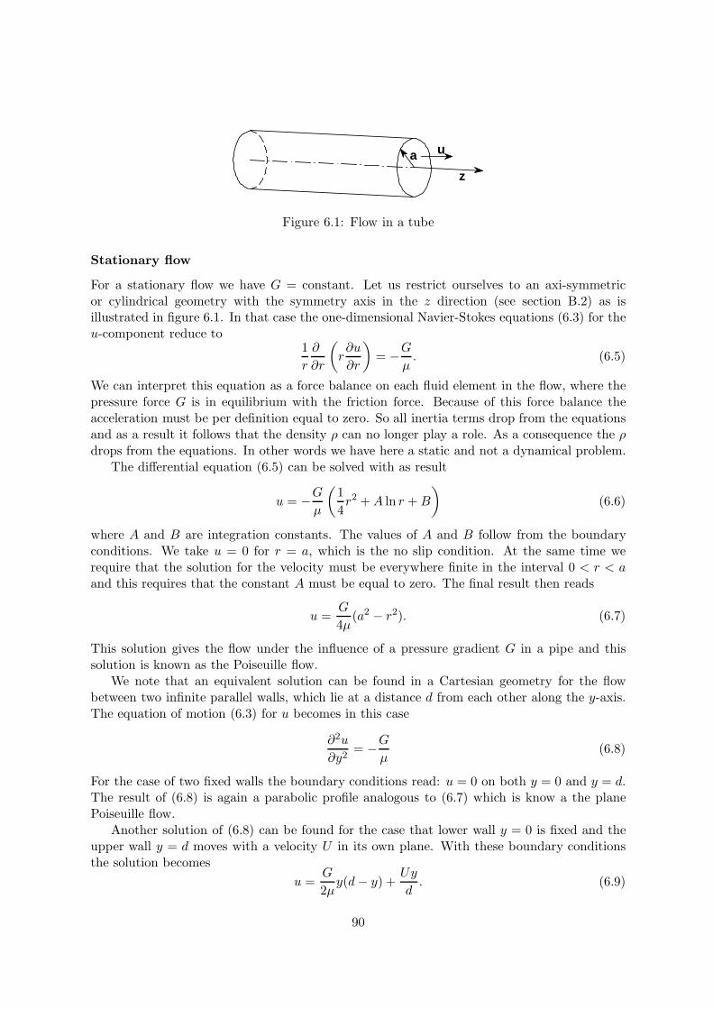
z

ua

Figure 6.1: Flow in a tube

Stationary flow

For a stationary flow we have G = constant. Let us restrict ourselves to an axi-symmetricor cylindrical geometry with the symmetry axis in the z direction (see section B.2) as isillustrated in figure 6.1. In that case the one-dimensional Navier-Stokes equations (6.3) for theu-component reduce to

1r

∂

∂r

(r∂u

∂r

)= −G

µ. (6.5)

We can interpret this equation as a force balance on each fluid element in the flow, where thepressure force G is in equilibrium with the friction force. Because of this force balance theacceleration must be per definition equal to zero. So all inertia terms drop from the equationsand as a result it follows that the density ρ can no longer play a role. As a consequence the ρdrops from the equations. In other words we have here a static and not a dynamical problem.

The differential equation (6.5) can be solved with as result

u = −Gµ

(14r2 +A ln r +B

)(6.6)

where A and B are integration constants. The values of A and B follow from the boundaryconditions. We take u = 0 for r = a, which is the no slip condition. At the same time werequire that the solution for the velocity must be everywhere finite in the interval 0 < r < aand this requires that the constant A must be equal to zero. The final result then reads

u =G

4µ(a2 − r2). (6.7)

This solution gives the flow under the influence of a pressure gradient G in a pipe and thissolution is known as the Poiseuille flow.

We note that an equivalent solution can be found in a Cartesian geometry for the flowbetween two infinite parallel walls, which lie at a distance d from each other along the y-axis.The equation of motion (6.3) for u becomes in this case

∂2u

∂y2= −G

µ(6.8)

For the case of two fixed walls the boundary conditions read: u = 0 on both y = 0 and y = d.The result of (6.8) is again a parabolic profile analogous to (6.7) which is know a the planePoiseuille flow.

Another solution of (6.8) can be found for the case that lower wall y = 0 is fixed and theupper wall y = d moves with a velocity U in its own plane. With these boundary conditionsthe solution becomes

u =G

2µy(d− y) +

Uy

d. (6.9)

90

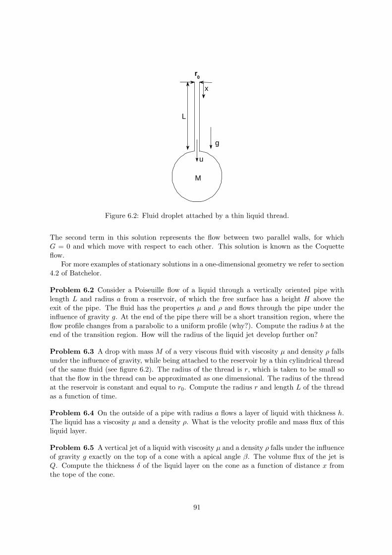
M

x

u

g

L

r0

Figure 6.2: Fluid droplet attached by a thin liquid thread.

The second term in this solution represents the flow between two parallel walls, for whichG = 0 and which move with respect to each other. This solution is known as the Coquetteflow.

For more examples of stationary solutions in a one-dimensional geometry we refer to section4.2 of Batchelor.

Problem 6.2 Consider a Poiseuille flow of a liquid through a vertically oriented pipe withlength L and radius a from a reservoir, of which the free surface has a height H above theexit of the pipe. The fluid has the properties µ and ρ and flows through the pipe under theinfluence of gravity g. At the end of the pipe there will be a short transition region, where theflow profile changes from a parabolic to a uniform profile (why?). Compute the radius b at theend of the transition region. How will the radius of the liquid jet develop further on?

Problem 6.3 A drop with mass M of a very viscous fluid with viscosity µ and density ρ fallsunder the influence of gravity, while being attached to the reservoir by a thin cylindrical threadof the same fluid (see figure 6.2). The radius of the thread is r, which is taken to be small sothat the flow in the thread can be approximated as one dimensional. The radius of the threadat the reservoir is constant and equal to r0. Compute the radius r and length L of the threadas a function of time.

Problem 6.4 On the outside of a pipe with radius a flows a layer of liquid with thickness h.The liquid has a viscosity µ and a density ρ. What is the velocity profile and mass flux of thisliquid layer.

Problem 6.5 A vertical jet of a liquid with viscosity µ and a density ρ falls under the influenceof gravity g exactly on the top of a cone with a apical angle β. The volume flux of the jet isQ. Compute the thickness δ of the liquid layer on the cone as a function of distance x fromthe tope of the cone.

91

Problem 6.6 Two immiscible viscous fluids, one with density ρ1 and viscosity µ1 and theother with density ρ2 and viscosity µ2 where ρ1 < ρ2, flow due to gravity down an incline,which makes an angle α with the horizontal. Fluid 1 lies on top of fluid 2. The upper fluidhas a depth h1 and the lower a depth h2. Compute the velocity profile as a function of thecoordinate y perpendicular to the incline. Compute also the dispersion relation of small waveson the interface.

Problem 6.7 Consider the two-dimensional flow between two parallel plates under the in-fluence of a pressure gradient for a so-called power-law fluid, for which the shear stress as afunction of the shear rate is given by

τxy = k

(∂u

∂y

)n

where k and n are constants. Compute the profile for various values of n both smaller than1 (a shear-thinning fluid) and larger than 1 (a shear-thickening fluid) and compare the resultwith the Couette flow for a Newtonian fluid.

Problem 6.8 Consider the two-dimensional flow between two parallel plates under the in-fluence of a pressure gradient for a so-called Bingham fluid, for which the shear stress as afunction of the shear rate is given by

τxy = µ∂u

∂yfor τxy > τ0

τxy = 0 for τxy < τ0

where τ0 is called the yield stress Compute the velocity profile and compare the result withthe Couette flow for a Newtonian fluid.

Instationary flow

To simplify the discussion we take in this case G = 0, which means that there is no externalforcing of the flow. For the equations of motion (6.3) the follows

∂u

∂t= ν

(∂2u

∂y2+∂2u

∂z2

). (6.10)

This is a familiar equation in mathematical physics which is known as the diffusion equationand which, as the name indicates, describes a diffusion process.

As an example of the solution of the diffusion equation (6.10) we consider the followingproblem. At time t = 0 we impose the following initial conditions

u = U , y > 0u = −U , y < 0 (6.11)

as is illustrated in figure 6.3. This geometry represents a tangential velocity discontinuity atthe position y = 0. In section 2.4.2 we have derived that such a velocity discontinuity canbe also interpreted as a vortex sheet at y=0. This is a geometry, in which all vorticity isconcentrated in a plane and where the strength of the vortex sheet is given by Γ = 2U .

92

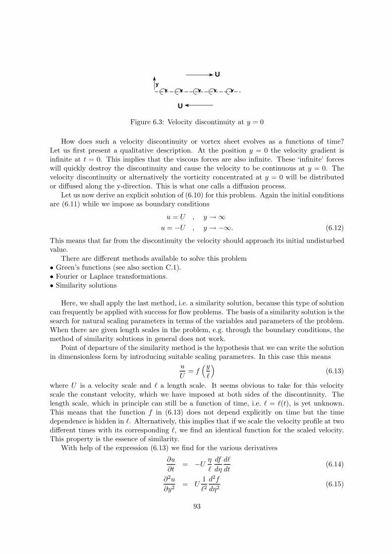
U

U

y

Figure 6.3: Velocity discontinuity at y = 0

How does such a velocity discontinuity or vortex sheet evolves as a functions of time?Let us first present a qualitative description. At the position y = 0 the velocity gradient isinfinite at t = 0. This implies that the viscous forces are also infinite. These ‘infinite’ forceswill quickly destroy the discontinuity and cause the velocity to be continuous at y = 0. Thevelocity discontinuity or alternatively the vorticity concentrated at y = 0 will be distributedor diffused along the y-direction. This is what one calls a diffusion process.

Let us now derive an explicit solution of (6.10) for this problem. Again the initial conditionsare (6.11) while we impose as boundary conditions

u = U , y → ∞u = −U , y → −∞. (6.12)

This means that far from the discontinuity the velocity should approach its initial undisturbedvalue.

There are different methods available to solve this problem• Green’s functions (see also section C.1).• Fourier or Laplace transformations.• Similarity solutions

Here, we shall apply the last method, i.e. a similarity solution, because this type of solutioncan frequently be applied with success for flow problems. The basis of a similarity solution is thesearch for natural scaling parameters in terms of the variables and parameters of the problem.When there are given length scales in the problem, e.g. through the boundary conditions, themethod of similarity solutions in general does not work.

Point of departure of the similarity method is the hypothesis that we can write the solutionin dimensionless form by introducing suitable scaling parameters. In this case this means

u

U= f

(y

)(6.13)

where U is a velocity scale and a length scale. It seems obvious to take for this velocityscale the constant velocity, which we have imposed at both sides of the discontinuity. Thelength scale, which in principle can still be a function of time, i.e. = (t), is yet unknown.This means that the function f in (6.13) does not depend explicitly on time but the timedependence is hidden in . Alternatively, this implies that if we scale the velocity profile at twodifferent times with its corresponding , we find an identical function for the scaled velocity.This property is the essence of similarity.

With help of the expression (6.13) we find for the various derivatives

∂u

∂t= −U η

df

dη

d

dt(6.14)

∂2u

∂y2= U

12d2f

dη2(6.15)

93

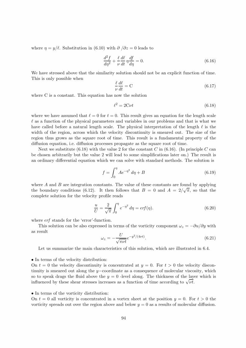
where η = y/. Substitution in (6.10) with ∂ /∂z = 0 leads to

d2f

dη2+

ν

d

dtηdf

dη= 0. (6.16)

We have stressed above that the similarity solution should not be an explicit function of time.This is only possible when

ν

d

dt= C (6.17)

where C is a constant. This equation has now the solution

2 = 2Cνt (6.18)

where we have assumed that = 0 for t = 0. This result gives an equation for the length scale as a function of the physical parameters and variables in our problems and that is what wehave called before a natural length scale. The physical interpretation of the length is thewidth of the region, across which the velocity discontinuity is smeared out. The size of theregion thus grows as the square root of time. This result is a fundamental property of thediffusion equation, i.e. diffusion processes propagate as the square root of time.

Next we substitute (6.18) with the value 2 for the constant C in (6.16). (In principle C canbe chosen arbitrarily but the value 2 will lead to some simplifications later on.) The result isan ordinary differential equation which we can solve with standard methods. The solution is

f =∫ η

0Ae−η2

dη +B (6.19)

where A and B are integration constants. The value of these constants are found by applyingthe boundary conditions (6.12). It then follows that B = 0 and A = 2/

√π, so that the

complete solution for the velocity profile reads

u

U=

2√π

∫ η

0e−η2

dη = erf(η). (6.20)

where erf stands for the ‘error’-function.This solution can be also expressed in terms of the vorticity component ωz = −∂u/∂y with

as resultωz = − U√

πνte−y2/(4νt). (6.21)

Let us summarize the main characteristics of this solution, which are illustrated in 6.4.

• In terms of the velocity distribution:On t = 0 the velocity discontinuity is concentrated at y = 0. For t > 0 the velocity discon-tinuity is smeared out along the y−coordinate as a consequence of molecular viscosity, whichso to speak drags the fluid above the y = 0 -level along. The thickness of the layer which isinfluenced by these shear stresses increases as a function of time according to

√νt.

• In terms of the vorticity distribution:On t = 0 all vorticity is concentrated in a vortex sheet at the position y = 0. For t > 0 thevorticity spreads out over the region above and below y = 0 as a results of molecular diffusion.

94

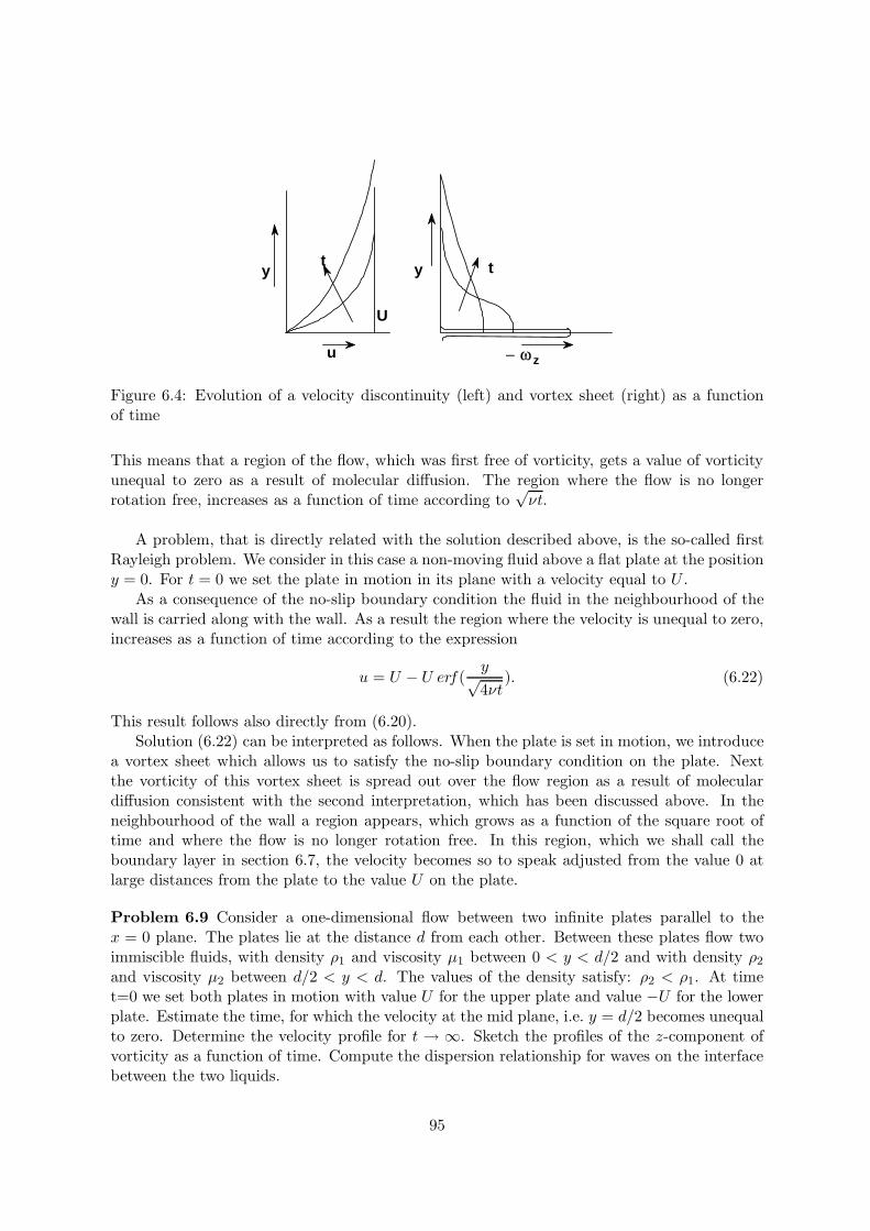
y yt t

U

u z− ω

Figure 6.4: Evolution of a velocity discontinuity (left) and vortex sheet (right) as a functionof time

This means that a region of the flow, which was first free of vorticity, gets a value of vorticityunequal to zero as a result of molecular diffusion. The region where the flow is no longerrotation free, increases as a function of time according to

√νt.

A problem, that is directly related with the solution described above, is the so-called firstRayleigh problem. We consider in this case a non-moving fluid above a flat plate at the positiony = 0. For t = 0 we set the plate in motion in its plane with a velocity equal to U .

As a consequence of the no-slip boundary condition the fluid in the neighbourhood of thewall is carried along with the wall. As a result the region where the velocity is unequal to zero,increases as a function of time according to the expression

u = U − U erf(y√4νt

). (6.22)

This result follows also directly from (6.20).Solution (6.22) can be interpreted as follows. When the plate is set in motion, we introduce

a vortex sheet which allows us to satisfy the no-slip boundary condition on the plate. Nextthe vorticity of this vortex sheet is spread out over the flow region as a result of moleculardiffusion consistent with the second interpretation, which has been discussed above. In theneighbourhood of the wall a region appears, which grows as a function of the square root oftime and where the flow is no longer rotation free. In this region, which we shall call theboundary layer in section 6.7, the velocity becomes so to speak adjusted from the value 0 atlarge distances from the plate to the value U on the plate.

Problem 6.9 Consider a one-dimensional flow between two infinite plates parallel to thex = 0 plane. The plates lie at the distance d from each other. Between these plates flow twoimmiscible fluids, with density ρ1 and viscosity µ1 between 0 < y < d/2 and with density ρ2

and viscosity µ2 between d/2 < y < d. The values of the density satisfy: ρ2 < ρ1. At timet=0 we set both plates in motion with value U for the upper plate and value −U for the lowerplate. Estimate the time, for which the velocity at the mid plane, i.e. y = d/2 becomes unequalto zero. Determine the velocity profile for t → ∞. Sketch the profiles of the z-component ofvorticity as a function of time. Compute the dispersion relationship for waves on the interfacebetween the two liquids.

95

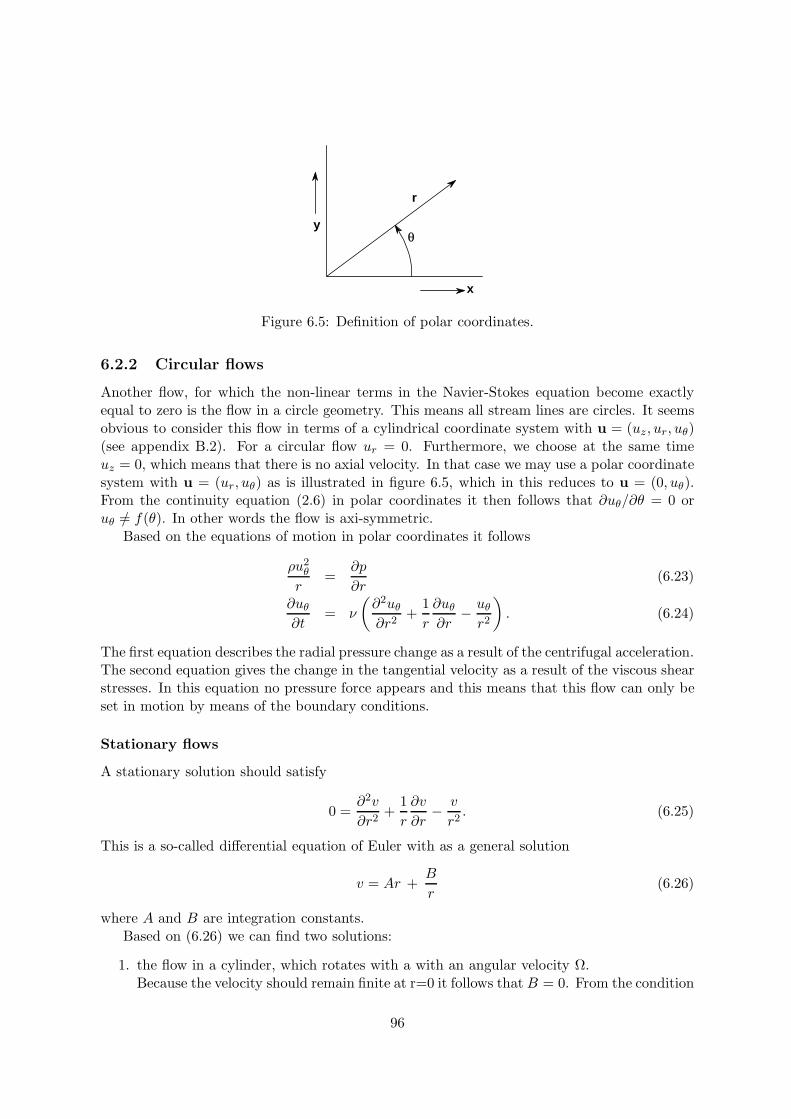
r

x

yθ

Figure 6.5: Definition of polar coordinates.

6.2.2 Circular flows

Another flow, for which the non-linear terms in the Navier-Stokes equation become exactlyequal to zero is the flow in a circle geometry. This means all stream lines are circles. It seemsobvious to consider this flow in terms of a cylindrical coordinate system with u = (uz, ur, uθ)(see appendix B.2). For a circular flow ur = 0. Furthermore, we choose at the same timeuz = 0, which means that there is no axial velocity. In that case we may use a polar coordinatesystem with u = (ur, uθ) as is illustrated in figure 6.5, which in this reduces to u = (0, uθ).From the continuity equation (2.6) in polar coordinates it then follows that ∂uθ/∂θ = 0 oruθ =/ f(θ). In other words the flow is axi-symmetric.

Based on the equations of motion in polar coordinates it follows

ρu2θ

r=

∂p

∂r(6.23)

∂uθ

∂t= ν

(∂2uθ

∂r2+

1r

∂uθ

∂r− uθ

r2

). (6.24)

The first equation describes the radial pressure change as a result of the centrifugal acceleration.The second equation gives the change in the tangential velocity as a result of the viscous shearstresses. In this equation no pressure force appears and this means that this flow can only beset in motion by means of the boundary conditions.

Stationary flows

A stationary solution should satisfy

0 =∂2v

∂r2+

1r

∂v

∂r− v

r2. (6.25)

This is a so-called differential equation of Euler with as a general solution

v = Ar +B

r(6.26)

where A and B are integration constants.Based on (6.26) we can find two solutions:

1. the flow in a cylinder, which rotates with a with an angular velocity Ω.Because the velocity should remain finite at r=0 it follows that B = 0. From the condition

96

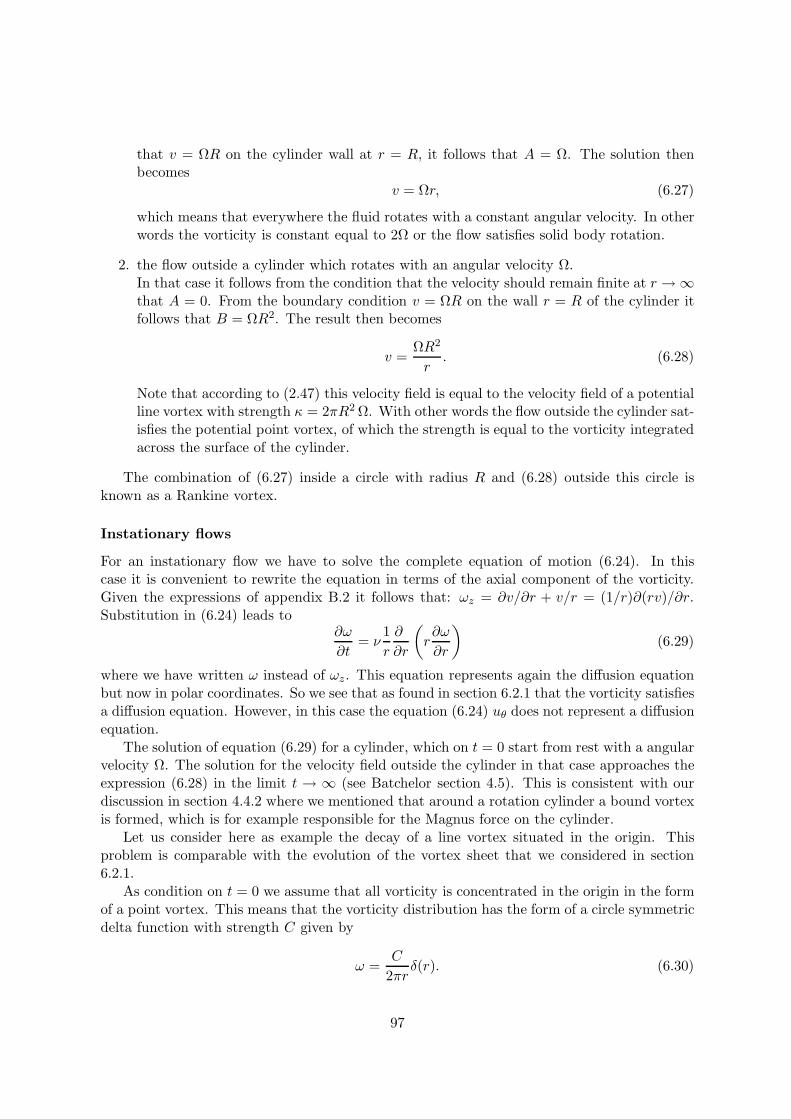
that v = ΩR on the cylinder wall at r = R, it follows that A = Ω. The solution thenbecomes

v = Ωr, (6.27)

which means that everywhere the fluid rotates with a constant angular velocity. In otherwords the vorticity is constant equal to 2Ω or the flow satisfies solid body rotation.

2. the flow outside a cylinder which rotates with an angular velocity Ω.In that case it follows from the condition that the velocity should remain finite at r → ∞that A = 0. From the boundary condition v = ΩR on the wall r = R of the cylinder itfollows that B = ΩR2. The result then becomes

v =ΩR2

r. (6.28)

Note that according to (2.47) this velocity field is equal to the velocity field of a potentialline vortex with strength κ = 2πR2 Ω. With other words the flow outside the cylinder sat-isfies the potential point vortex, of which the strength is equal to the vorticity integratedacross the surface of the cylinder.

The combination of (6.27) inside a circle with radius R and (6.28) outside this circle isknown as a Rankine vortex.

Instationary flows

For an instationary flow we have to solve the complete equation of motion (6.24). In thiscase it is convenient to rewrite the equation in terms of the axial component of the vorticity.Given the expressions of appendix B.2 it follows that: ωz = ∂v/∂r + v/r = (1/r)∂(rv)/∂r.Substitution in (6.24) leads to

∂ω

∂t= ν

1r

∂

∂r

(r∂ω

∂r

)(6.29)

where we have written ω instead of ωz. This equation represents again the diffusion equationbut now in polar coordinates. So we see that as found in section 6.2.1 that the vorticity satisfiesa diffusion equation. However, in this case the equation (6.24) uθ does not represent a diffusionequation.

The solution of equation (6.29) for a cylinder, which on t = 0 start from rest with a angularvelocity Ω. The solution for the velocity field outside the cylinder in that case approaches theexpression (6.28) in the limit t → ∞ (see Batchelor section 4.5). This is consistent with ourdiscussion in section 4.4.2 where we mentioned that around a rotation cylinder a bound vortexis formed, which is for example responsible for the Magnus force on the cylinder.

Let us consider here as example the decay of a line vortex situated in the origin. Thisproblem is comparable with the evolution of the vortex sheet that we considered in section6.2.1.

As condition on t = 0 we assume that all vorticity is concentrated in the origin in the formof a point vortex. This means that the vorticity distribution has the form of a circle symmetricdelta function with strength C given by

ω =C

2πrδ(r). (6.30)

97

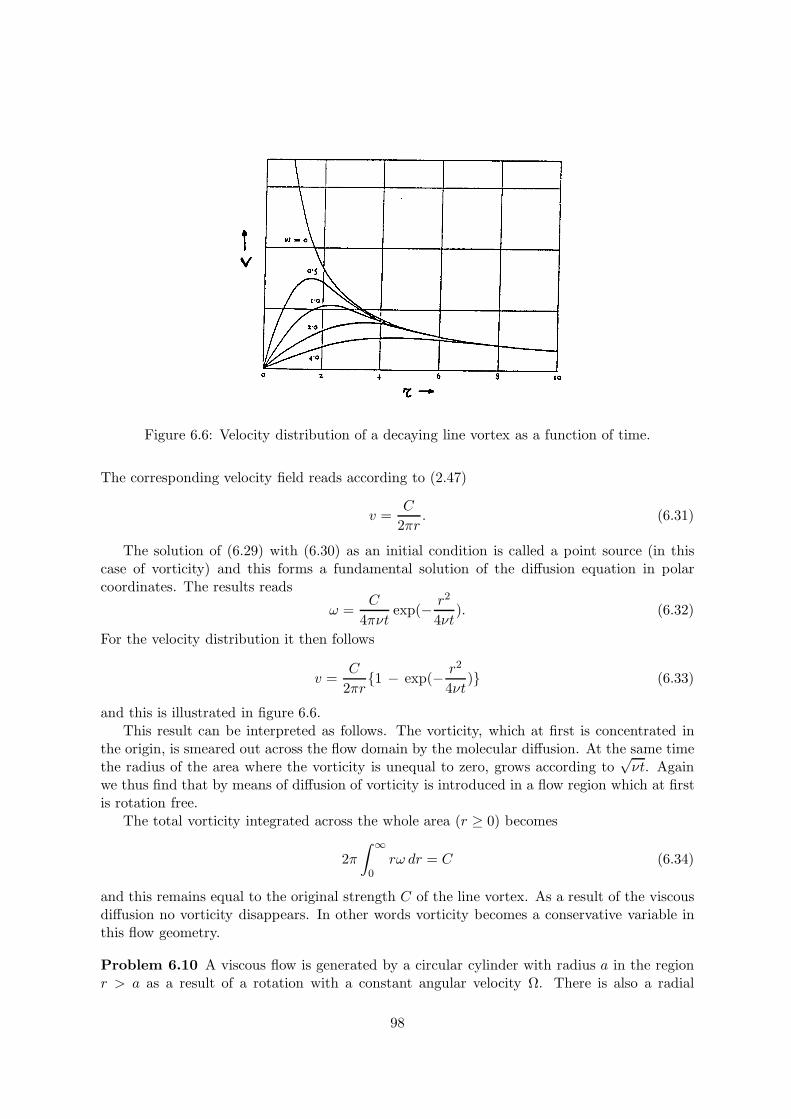
Figure 6.6: Velocity distribution of a decaying line vortex as a function of time.

The corresponding velocity field reads according to (2.47)

v =C

2πr. (6.31)

The solution of (6.29) with (6.30) as an initial condition is called a point source (in thiscase of vorticity) and this forms a fundamental solution of the diffusion equation in polarcoordinates. The results reads

ω =C

4πνtexp(− r2

4νt). (6.32)

For the velocity distribution it then follows

v =C

2πr1 − exp(− r2

4νt) (6.33)

and this is illustrated in figure 6.6.This result can be interpreted as follows. The vorticity, which at first is concentrated in

the origin, is smeared out across the flow domain by the molecular diffusion. At the same timethe radius of the area where the vorticity is unequal to zero, grows according to

√νt. Again

we thus find that by means of diffusion of vorticity is introduced in a flow region which at firstis rotation free.

The total vorticity integrated across the whole area (r ≥ 0) becomes

2π∫ ∞

0rω dr = C (6.34)

and this remains equal to the original strength C of the line vortex. As a result of the viscousdiffusion no vorticity disappears. In other words vorticity becomes a conservative variable inthis flow geometry.

Problem 6.10 A viscous flow is generated by a circular cylinder with radius a in the regionr > a as a result of a rotation with a constant angular velocity Ω. There is also a radial

98

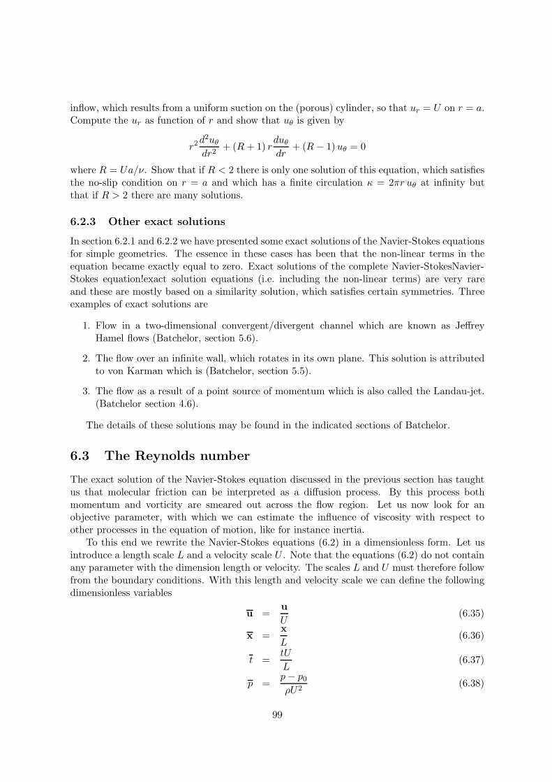
inflow, which results from a uniform suction on the (porous) cylinder, so that ur = U on r = a.Compute the ur as function of r and show that uθ is given by

r2d2uθ

dr2+ (R+ 1) r

duθ

dr+ (R− 1) uθ = 0

where R = Ua/ν. Show that if R < 2 there is only one solution of this equation, which satisfiesthe no-slip condition on r = a and which has a finite circulation κ = 2πr uθ at infinity butthat if R > 2 there are many solutions.

6.2.3 Other exact solutions

In section 6.2.1 and 6.2.2 we have presented some exact solutions of the Navier-Stokes equationsfor simple geometries. The essence in these cases has been that the non-linear terms in theequation became exactly equal to zero. Exact solutions of the complete Navier-StokesNavier-Stokes equation!exact solution equations (i.e. including the non-linear terms) are very rareand these are mostly based on a similarity solution, which satisfies certain symmetries. Threeexamples of exact solutions are

1. Flow in a two-dimensional convergent/divergent channel which are known as JeffreyHamel flows (Batchelor, section 5.6).

2. The flow over an infinite wall, which rotates in its own plane. This solution is attributedto von Karman which is (Batchelor, section 5.5).

3. The flow as a result of a point source of momentum which is also called the Landau-jet.(Batchelor section 4.6).

The details of these solutions may be found in the indicated sections of Batchelor.

6.3 The Reynolds number

The exact solution of the Navier-Stokes equation discussed in the previous section has taughtus that molecular friction can be interpreted as a diffusion process. By this process bothmomentum and vorticity are smeared out across the flow region. Let us now look for anobjective parameter, with which we can estimate the influence of viscosity with respect toother processes in the equation of motion, like for instance inertia.

To this end we rewrite the Navier-Stokes equations (6.2) in a dimensionless form. Let usintroduce a length scale L and a velocity scale U . Note that the equations (6.2) do not containany parameter with the dimension length or velocity. The scales L and U must therefore followfrom the boundary conditions. With this length and velocity scale we can define the followingdimensionless variables

u =uU

(6.35)

x =xL

(6.36)

t =tU

L(6.37)

p =p− p0

ρU2(6.38)

99

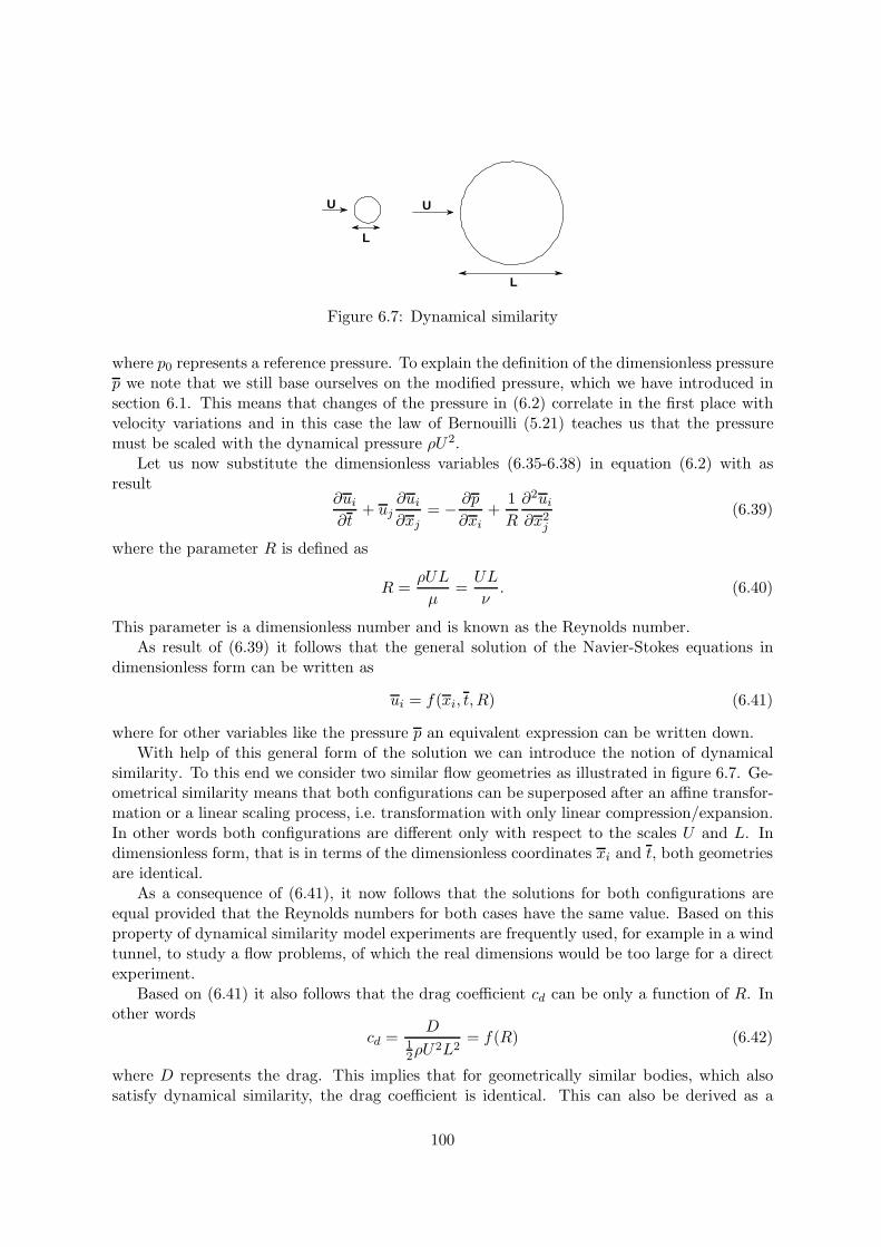
L

U

L

U

Figure 6.7: Dynamical similarity

where p0 represents a reference pressure. To explain the definition of the dimensionless pressurep we note that we still base ourselves on the modified pressure, which we have introduced insection 6.1. This means that changes of the pressure in (6.2) correlate in the first place withvelocity variations and in this case the law of Bernouilli (5.21) teaches us that the pressuremust be scaled with the dynamical pressure ρU2.

Let us now substitute the dimensionless variables (6.35-6.38) in equation (6.2) with asresult

∂ui

∂t+ uj

∂ui

∂xj= − ∂p

∂xi+

1R

∂2ui

∂x2j

(6.39)

where the parameter R is defined as

R =ρUL

µ=UL

ν. (6.40)

This parameter is a dimensionless number and is known as the Reynolds number.As result of (6.39) it follows that the general solution of the Navier-Stokes equations in

dimensionless form can be written as

ui = f(xi, t, R) (6.41)

where for other variables like the pressure p an equivalent expression can be written down.With help of this general form of the solution we can introduce the notion of dynamical

similarity. To this end we consider two similar flow geometries as illustrated in figure 6.7. Ge-ometrical similarity means that both configurations can be superposed after an affine transfor-mation or a linear scaling process, i.e. transformation with only linear compression/expansion.In other words both configurations are different only with respect to the scales U and L. Indimensionless form, that is in terms of the dimensionless coordinates xi and t, both geometriesare identical.

As a consequence of (6.41), it now follows that the solutions for both configurations areequal provided that the Reynolds numbers for both cases have the same value. Based on thisproperty of dynamical similarity model experiments are frequently used, for example in a windtunnel, to study a flow problems, of which the real dimensions would be too large for a directexperiment.

Based on (6.41) it also follows that the drag coefficient cd can be only a function of R. Inother words

cd =D

12ρU

2L2= f(R) (6.42)

where D represents the drag. This implies that for geometrically similar bodies, which alsosatisfy dynamical similarity, the drag coefficient is identical. This can also be derived as a

100

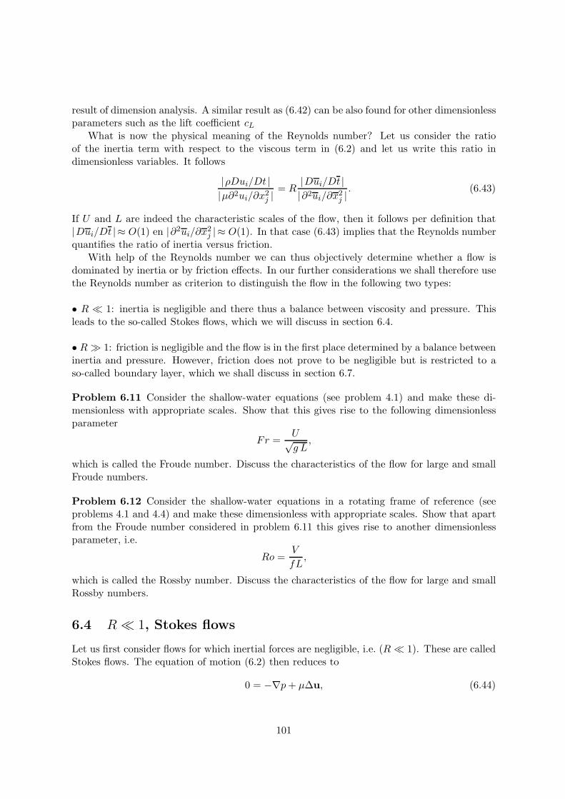
result of dimension analysis. A similar result as (6.42) can be also found for other dimensionlessparameters such as the lift coefficient cL

What is now the physical meaning of the Reynolds number? Let us consider the ratioof the inertia term with respect to the viscous term in (6.2) and let us write this ratio indimensionless variables. It follows

|ρDui/Dt ||µ∂2ui/∂x2

j |= R

|Dui/Dt ||∂2ui/∂x2

j |. (6.43)

If U and L are indeed the characteristic scales of the flow, then it follows per definition that|Dui/Dt | ≈ O(1) en |∂2ui/∂x

2j | ≈ O(1). In that case (6.43) implies that the Reynolds number

quantifies the ratio of inertia versus friction.With help of the Reynolds number we can thus objectively determine whether a flow is

dominated by inertia or by friction effects. In our further considerations we shall therefore usethe Reynolds number as criterion to distinguish the flow in the following two types:

• R 1: inertia is negligible and there thus a balance between viscosity and pressure. Thisleads to the so-called Stokes flows, which we will discuss in section 6.4.

• R 1: friction is negligible and the flow is in the first place determined by a balance betweeninertia and pressure. However, friction does not prove to be negligible but is restricted to aso-called boundary layer, which we shall discuss in section 6.7.

Problem 6.11 Consider the shallow-water equations (see problem 4.1) and make these di-mensionless with appropriate scales. Show that this gives rise to the following dimensionlessparameter

Fr =U√g L

,

which is called the Froude number. Discuss the characteristics of the flow for large and smallFroude numbers.

Problem 6.12 Consider the shallow-water equations in a rotating frame of reference (seeproblems 4.1 and 4.4) and make these dimensionless with appropriate scales. Show that apartfrom the Froude number considered in problem 6.11 this gives rise to another dimensionlessparameter, i.e.

Ro =V

fL,

which is called the Rossby number. Discuss the characteristics of the flow for large and smallRossby numbers.

6.4 R 1, Stokes flows

Let us first consider flows for which inertial forces are negligible, i.e. (R 1). These are calledStokes flows. The equation of motion (6.2) then reduces to

0 = −∇p+ µ∆u, (6.44)

101

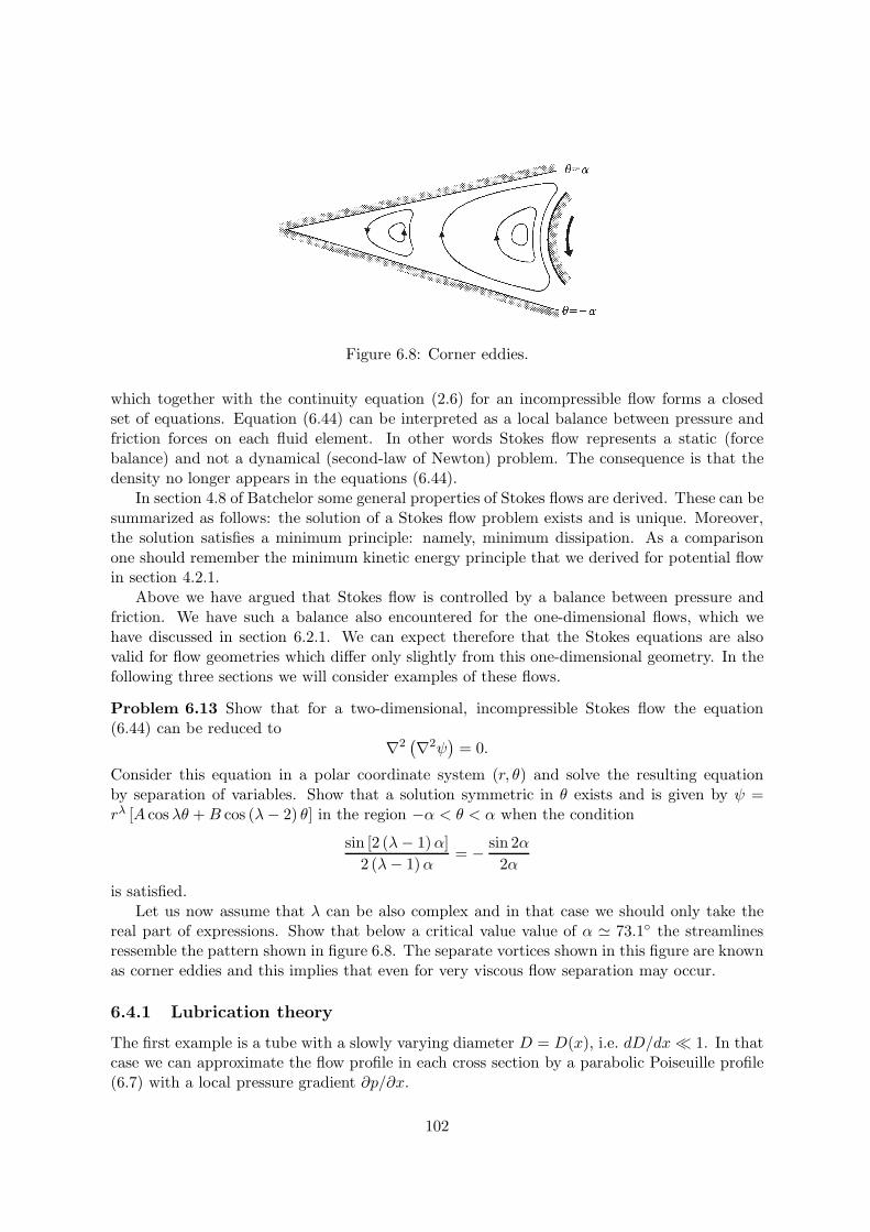
Figure 6.8: Corner eddies.

which together with the continuity equation (2.6) for an incompressible flow forms a closedset of equations. Equation (6.44) can be interpreted as a local balance between pressure andfriction forces on each fluid element. In other words Stokes flow represents a static (forcebalance) and not a dynamical (second-law of Newton) problem. The consequence is that thedensity no longer appears in the equations (6.44).

In section 4.8 of Batchelor some general properties of Stokes flows are derived. These can besummarized as follows: the solution of a Stokes flow problem exists and is unique. Moreover,the solution satisfies a minimum principle: namely, minimum dissipation. As a comparisonone should remember the minimum kinetic energy principle that we derived for potential flowin section 4.2.1.

Above we have argued that Stokes flow is controlled by a balance between pressure andfriction. We have such a balance also encountered for the one-dimensional flows, which wehave discussed in section 6.2.1. We can expect therefore that the Stokes equations are alsovalid for flow geometries which differ only slightly from this one-dimensional geometry. In thefollowing three sections we will consider examples of these flows.

Problem 6.13 Show that for a two-dimensional, incompressible Stokes flow the equation(6.44) can be reduced to

∇2(∇2ψ

)= 0.

Consider this equation in a polar coordinate system (r, θ) and solve the resulting equationby separation of variables. Show that a solution symmetric in θ exists and is given by ψ =rλ [A cos λθ +B cos (λ− 2) θ] in the region −α < θ < α when the condition

sin [2 (λ− 1)α]2 (λ− 1)α

= − sin 2α2α

is satisfied.Let us now assume that λ can be also complex and in that case we should only take the

real part of expressions. Show that below a critical value value of α 73.1 the streamlinesressemble the pattern shown in figure 6.8. The separate vortices shown in this figure are knownas corner eddies and this implies that even for very viscous flow separation may occur.

6.4.1 Lubrication theory

The first example is a tube with a slowly varying diameter D = D(x), i.e. dD/dx 1. In thatcase we can approximate the flow profile in each cross section by a parabolic Poiseuille profile(6.7) with a local pressure gradient ∂p/∂x.

102

Next we compute the volume flow Q, which is transported through each cross section ofthe pipe and which reads

Q =∫ D/2

0u 2πr dr

= − πD4

128µ∂p

∂x(6.45)

where we have used (6.7) to compute Q.Continuity or alternatively conservation of mass requires that through each cross section

per unit time the same amount of fluid must pass or in other words Q =/ f(x). Because D isknown, we can interpret (6.45) as a differential equation for the pressure, which we can solvewhen the variation of D as function of x is known.

Let us consider as an example the case when diameter D varies linearly between the valuesD0 and D1 over a distance L, i.e.

D = D0 + (D1 −D0)x

L= D0

(1 + ε

x

L

). (6.46)

In order to satisfy the condition that the cross section varies slowly, we must assume ε ≡(D1 −D0) /D0 1. Substitution in (6.45) and integration then leads to

pL − p0 =1283

µL

επD40

Q

(1 − 1

(1 + ε)3

). (6.47)

When the pressure difference pL−p0 is given for instance as a boundary condition, (6.47) givesan expression for the volume flow Q. With this value for Q we can then obtain the pressureat an arbitrary position x along the pipe by integrating (6.45) between 0 and x which leads to

px − p0 =1283

µL

επD40

Q

(1 − 1(

1 + ε xL

)3). (6.48)

By substitution of this pressure into the Poiseuille profile we can now compute the velocityprofile at each x-position.

Another example of this type of Stokes flow is the flow problem through a narrow diver-gent/convergent slit. This configuration appears for instance as a journal bearing and thisexplains the title (lubrication theory) of the section. For further details we refer to section 4.8of Batchelor.

Problem 6.14 A slider bearing consists of a flat plate moving with a constant velocity U inthe x-direction and a fixed slider at

y = h(1 − λ

x

L

)for 0 < x < L and 0 < λ < 1. Given that Uh2/(νL) 1 and the ambient pressure outside thebearing is p0, show that the pressure within the bearing is

p = p0 +6µULλx(L− x)

(2 − λ)h2(L− λx)2.

Show that the load supported by the bearing is

F =6µUL2

λ2 h2

[ln

11 − λ

− 2λ2 − λ

].

103

Figure 6.9: Journal bearing.

Problem 6.15 A cylindrical shaft of radius a rotates with a angular velocity ω within a fixedcylindrical housing (journal) of radius a(1+ ε). The gap between the cylinders is filled with oilof viscosity ν. Show that when the centre of the shaft is offset at a distance dε (d < a) fromthe centre of the journal, the gap is given by h(θ) = ε(a− d cos θ) when ε is small and θ is thepolar angle shown in figure 6.9. Deduce that the lubrication approximation is valid in the gapif ωa2ε2 ν. Hence show that the pressure satisfies

dp

dθ=

6(H −H0)H3

where H = 1 − d cos θ/a and H0 is a constant given by

H0 =

∫ 2π0

dθH2∫ 2π

0dθH3

.

Deduce that ∫ 2π

0p cos θ dθ = 0

and hence the force on the shaft is perpendicular to the line of centres (θ = 0). What are theimplications for the trajectory of the shaft (assuming it is unrestrained at its ends and thatthe journal is fixed)?

Problem 6.16 A squeeze film exists between two parallel plates of length L at y = 0 andy = δL. Starting at t = 0, a constant force is exerted downwards on the top plate. Showthat the correct scaling for the horizontal velocity is Fδ2/µ. Deduce that at time t later thedistance between the plates is

D =δL√

1 + αt

where α is to be determined. This predicts that the plates will not touch in finite time.Consider the validity of this prediction by computing roughly the time taken for the film toclose when the surface roughness (the ‘asperity’ size) has an amplitude 10−3δL.

Problem 6.17 A thin layer of rain water with viscosity ν is draining under the effects ofgravity down the side of a vertical flat windowpane. If the thickness of the layer h is a functiononly of time t and distance x down the pane, show that the lubrication theory approximationleads to h(x, t) satisfying the equation

∂h

∂t+gh2

ν

∂h

∂x= 0.

104

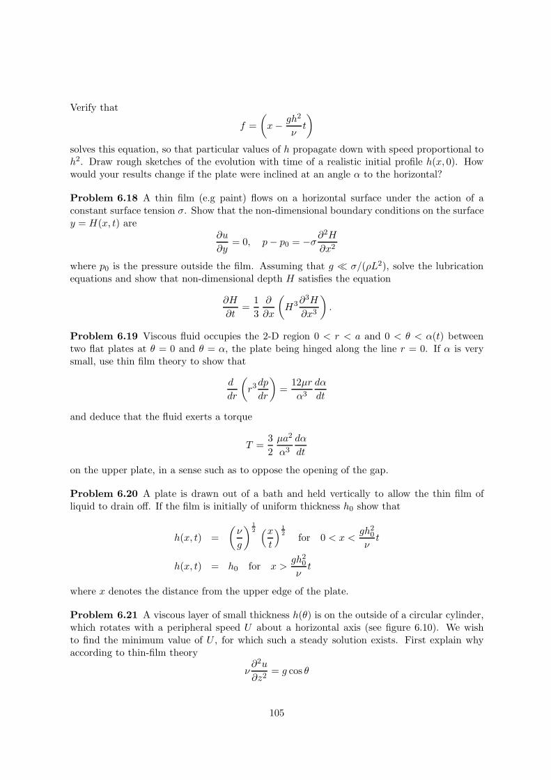
Verify that

f =(x− gh2

νt

)solves this equation, so that particular values of h propagate down with speed proportional toh2. Draw rough sketches of the evolution with time of a realistic initial profile h(x, 0). Howwould your results change if the plate were inclined at an angle α to the horizontal?

Problem 6.18 A thin film (e.g paint) flows on a horizontal surface under the action of aconstant surface tension σ. Show that the non-dimensional boundary conditions on the surfacey = H(x, t) are

∂u

∂y= 0, p− p0 = −σ∂

2H

∂x2

where p0 is the pressure outside the film. Assuming that g σ/(ρL2), solve the lubricationequations and show that non-dimensional depth H satisfies the equation

∂H

∂t=

13∂

∂x

(H3∂

3H

∂x3

).

Problem 6.19 Viscous fluid occupies the 2-D region 0 < r < a and 0 < θ < α(t) betweentwo flat plates at θ = 0 and θ = α, the plate being hinged along the line r = 0. If α is verysmall, use thin film theory to show that

d

dr

(r3dp

dr

)=

12µrα3

dα

dt

and deduce that the fluid exerts a torque

T =32µa2

α3

dα

dt

on the upper plate, in a sense such as to oppose the opening of the gap.

Problem 6.20 A plate is drawn out of a bath and held vertically to allow the thin film ofliquid to drain off. If the film is initially of uniform thickness h0 show that

h(x, t) =(ν

g

)12 (x

t

) 12 for 0 < x <

gh20

νt

h(x, t) = h0 for x >gh2

0

νt

where x denotes the distance from the upper edge of the plate.

Problem 6.21 A viscous layer of small thickness h(θ) is on the outside of a circular cylinder,which rotates with a peripheral speed U about a horizontal axis (see figure 6.10). We wishto find the minimum value of U , for which such a steady solution exists. First explain whyaccording to thin-film theory

ν∂2u

∂z2= g cos θ

105

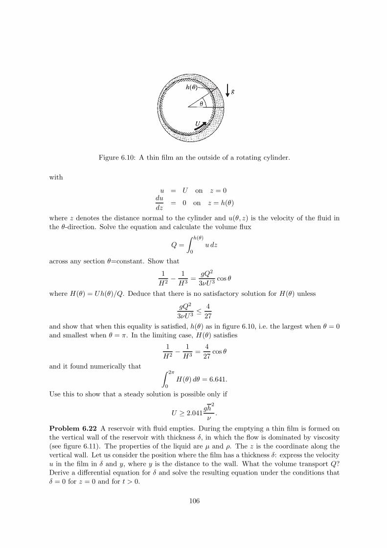
Figure 6.10: A thin film an the outside of a rotating cylinder.

with

u = U on z = 0du

dz= 0 on z = h(θ)

where z denotes the distance normal to the cylinder and u(θ, z) is the velocity of the fluid inthe θ-direction. Solve the equation and calculate the volume flux

Q =∫ h(θ)

0u dz

across any section θ=constant. Show that

1H2

− 1H3

=gQ2

3νU3cos θ

where H(θ) = Uh(θ)/Q. Deduce that there is no satisfactory solution for H(θ) unless

gQ2

3νU3≤ 4

27and show that when this equality is satisfied, h(θ) as in figure 6.10, i.e. the largest when θ = 0and smallest when θ = π. In the limiting case, H(θ) satisfies

1H2

− 1H3

=427

cos θ

and it found numerically that ∫ 2π

0H(θ) dθ = 6.641.

Use this to show that a steady solution is possible only if

U ≥ 2.041gh

2

ν.

Problem 6.22 A reservoir with fluid empties. During the emptying a thin film is formed onthe vertical wall of the reservoir with thickness δ, in which the flow is dominated by viscosity(see figure 6.11). The properties of the liquid are µ and ρ. The z is the coordinate along thevertical wall. Let us consider the position where the film has a thickness δ: express the velocityu in the film in δ and y, where y is the distance to the wall. What the volume transport Q?Derive a differential equation for δ and solve the resulting equation under the conditions thatδ = 0 for z = 0 and for t > 0.

106

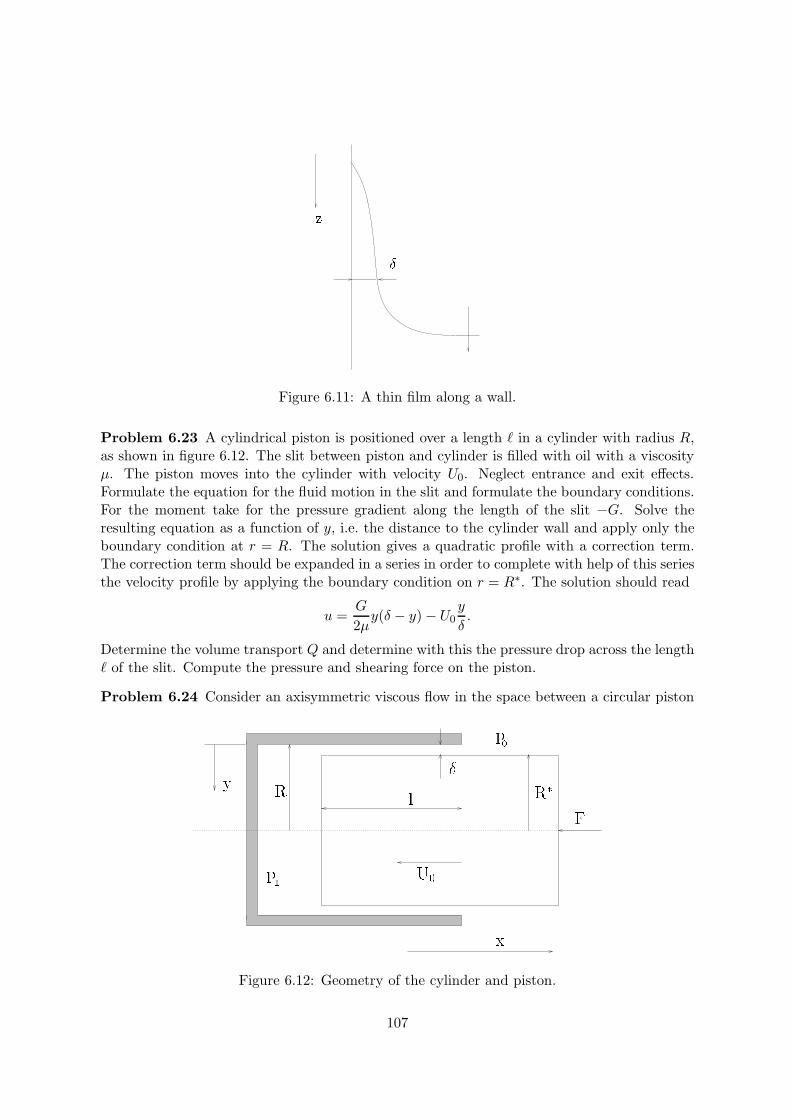
z

Figure 6.11: A thin film along a wall.

Problem 6.23 A cylindrical piston is positioned over a length in a cylinder with radius R,as shown in figure 6.12. The slit between piston and cylinder is filled with oil with a viscosityµ. The piston moves into the cylinder with velocity U0. Neglect entrance and exit effects.Formulate the equation for the fluid motion in the slit and formulate the boundary conditions.For the moment take for the pressure gradient along the length of the slit −G. Solve theresulting equation as a function of y, i.e. the distance to the cylinder wall and apply only theboundary condition at r = R. The solution gives a quadratic profile with a correction term.The correction term should be expanded in a series in order to complete with help of this seriesthe velocity profile by applying the boundary condition on r = R∗. The solution should read

u =G

2µy(δ − y) − U0

y

δ.

Determine the volume transport Q and determine with this the pressure drop across the length of the slit. Compute the pressure and shearing force on the piston.

Problem 6.24 Consider an axisymmetric viscous flow in the space between a circular piston

Rl

F

U

R

x

y

p

p

Figure 6.12: Geometry of the cylinder and piston.

107

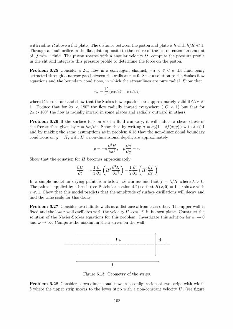
with radius R above a flat plate. The distance between the piston and plate is h with h/R 1.Through a small orifice in the flat plate opposite to the centre of the piston enters an amountof Q m3s−1 fluid. The piston rotates with a angular velocity Ω. compute the pressure profilein the slit and integrate this pressure profile to determine the force on the piston.

Problem 6.25 Consider a 2-D flow in a convergent channel, −α < θ < α the fluid beingextracted through a narrow gap between the walls at r = 0. Seek a solution to the Stokes flowequations and the boundary conditions, in which the streamlines are pure radial. Show that

ur =C

r(cos 2θ − cos 2α)

where C is constant and show that the Stokes flow equations are approximately valid if C/ν 1. Deduce that for 2α < 180 the flow radially inward everywhere ( C < 1) but that for2α > 180 the flow is radially inward in some places and radially outward in others.

Problem 6.26 If the surface tension σ of a fluid can vary, it will induce a shear stress inthe free surface given by τ = ∂σ/∂s. Show that by writing σ = σ0(1 + δf(x, y) ) with δ 1and by making the same assumptions as in problem 6.18 that the non-dimensional boundaryconditions on y = H, with H a non-dimensional depth, are approximately

p = −σ∂2H

∂x2, µ

∂u

∂y= τ.

Show that the equation for H becomes approximately

∂H

∂t= −1

3∂

∂x

(H3∂

3H

∂x3

)− 1

2∂

∂x

(H2∂f

∂x.

)

In a simple model for drying paint from below, we can assume that f = λ/H where λ > 0.The paint is applied by a brush (see Batchelor section 4.2) so that H(x, 0) = 1 + ε sin kx withε 1. Show that this model predicts that the amplitude of surface oscillations will decay andfind the time scale for this decay.

Problem 6.27 Consider two infinite walls at a distance d from each other. The upper wall isfixed and the lower wall oscillates with the velocity U0 cos(ωt) in its own plane. Construct thesolution of the Navier-Stokes equations for this problem. Investigate this solution for ω → 0and ω → ∞. Compute the maximum shear stress on the wall.

dU

b

Figure 6.13: Geometry of the strips.

Problem 6.28 Consider a two-dimensional flow in a configuration of two strips with widthb where the upper strip moves to the lower strip with a non-constant velocity U0 (see figure

108

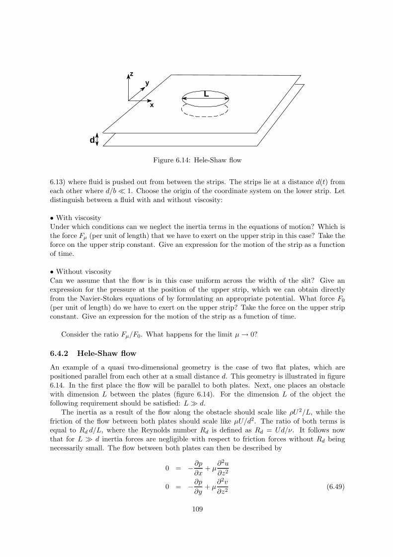
L

d

x

yz

Figure 6.14: Hele-Shaw flow

6.13) where fluid is pushed out from between the strips. The strips lie at a distance d(t) fromeach other where d/b 1. Choose the origin of the coordinate system on the lower strip. Letdistinguish between a fluid with and without viscosity:

• With viscosityUnder which conditions can we neglect the inertia terms in the equations of motion? Which isthe force Fµ (per unit of length) that we have to exert on the upper strip in this case? Take theforce on the upper strip constant. Give an expression for the motion of the strip as a functionof time.

• Without viscosityCan we assume that the flow is in this case uniform across the width of the slit? Give anexpression for the pressure at the position of the upper strip, which we can obtain directlyfrom the Navier-Stokes equations of by formulating an appropriate potential. What force F0

(per unit of length) do we have to exert on the upper strip? Take the force on the upper stripconstant. Give an expression for the motion of the strip as a function of time.

Consider the ratio Fµ/F0. What happens for the limit µ→ 0?

6.4.2 Hele-Shaw flow

An example of a quasi two-dimensional geometry is the case of two flat plates, which arepositioned parallel from each other at a small distance d. This geometry is illustrated in figure6.14. In the first place the flow will be parallel to both plates. Next, one places an obstaclewith dimension L between the plates (figure 6.14). For the dimension L of the object thefollowing requirement should be satisfied: L d.

The inertia as a result of the flow along the obstacle should scale like ρU2/L, while thefriction of the flow between both plates should scale like µU/d2. The ratio of both terms isequal to Rd d/L, where the Reynolds number Rd is defined as Rd = Ud/ν. It follows nowthat for L d inertia forces are negligible with respect to friction forces without Rd beingnecessarily small. The flow between both plates can then be described by

0 = −∂p∂x

+ µ∂2u

∂z2

0 = −∂p∂y

+ µ∂2v

∂z2(6.49)

109

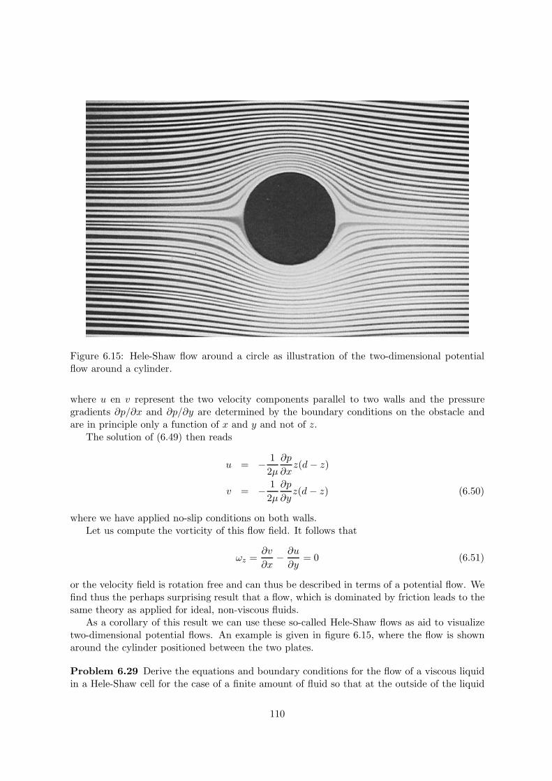
Figure 6.15: Hele-Shaw flow around a circle as illustration of the two-dimensional potentialflow around a cylinder.

where u en v represent the two velocity components parallel to two walls and the pressuregradients ∂p/∂x and ∂p/∂y are determined by the boundary conditions on the obstacle andare in principle only a function of x and y and not of z.

The solution of (6.49) then reads

u = − 12µ

∂p

∂xz(d− z)

v = − 12µ

∂p

∂yz(d − z) (6.50)

where we have applied no-slip conditions on both walls.Let us compute the vorticity of this flow field. It follows that

ωz =∂v

∂x− ∂u

∂y= 0 (6.51)

or the velocity field is rotation free and can thus be described in terms of a potential flow. Wefind thus the perhaps surprising result that a flow, which is dominated by friction leads to thesame theory as applied for ideal, non-viscous fluids.

As a corollary of this result we can use these so-called Hele-Shaw flows as aid to visualizetwo-dimensional potential flows. An example is given in figure 6.15, where the flow is shownaround the cylinder positioned between the two plates.

Problem 6.29 Derive the equations and boundary conditions for the flow of a viscous liquidin a Hele-Shaw cell for the case of a finite amount of fluid so that at the outside of the liquid

110

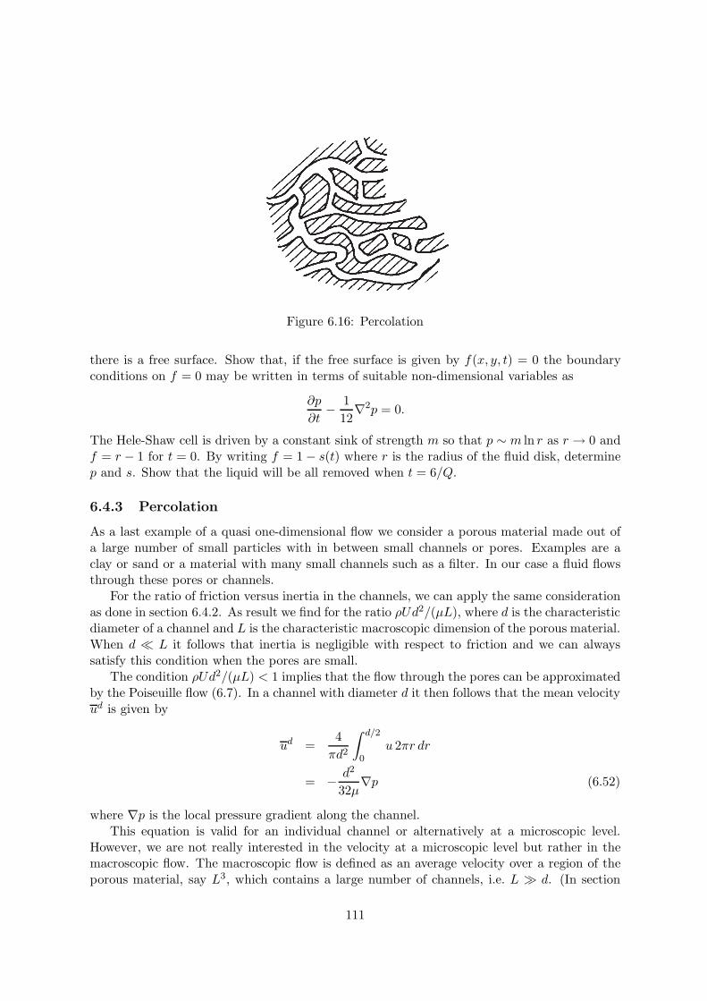
Figure 6.16: Percolation

there is a free surface. Show that, if the free surface is given by f(x, y, t) = 0 the boundaryconditions on f = 0 may be written in terms of suitable non-dimensional variables as

∂p

∂t− 1

12∇2p = 0.

The Hele-Shaw cell is driven by a constant sink of strength m so that p ∼ m ln r as r → 0 andf = r − 1 for t = 0. By writing f = 1 − s(t) where r is the radius of the fluid disk, determinep and s. Show that the liquid will be all removed when t = 6/Q.

6.4.3 Percolation

As a last example of a quasi one-dimensional flow we consider a porous material made out ofa large number of small particles with in between small channels or pores. Examples are aclay or sand or a material with many small channels such as a filter. In our case a fluid flowsthrough these pores or channels.

For the ratio of friction versus inertia in the channels, we can apply the same considerationas done in section 6.4.2. As result we find for the ratio ρUd2/(µL), where d is the characteristicdiameter of a channel and L is the characteristic macroscopic dimension of the porous material.When d L it follows that inertia is negligible with respect to friction and we can alwayssatisfy this condition when the pores are small.

The condition ρUd2/(µL) < 1 implies that the flow through the pores can be approximatedby the Poiseuille flow (6.7). In a channel with diameter d it then follows that the mean velocityud is given by

ud =4πd2

∫ d/2

0u 2πr dr

= − d2

32µ∇p (6.52)

where ∇p is the local pressure gradient along the channel.This equation is valid for an individual channel or alternatively at a microscopic level.

However, we are not really interested in the velocity at a microscopic level but rather in themacroscopic flow. The macroscopic flow is defined as an average velocity over a region of theporous material, say L3, which contains a large number of channels, i.e. L d. (In section

111

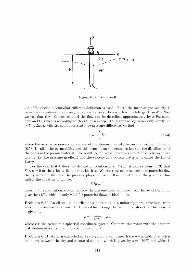
Figure 6.17: Water well

4.8 of Batchelor a somewhat different definition is used. There the macroscopic velocity isbased on the volume flux through a representative surface which is much larger than d2.) Nowwe use that through each channel the flow can be described approximately by a Poiseuilleflow and this means according to (6.7) that u ∼ ∇p. If the average ∇p varies only slowly, i.e|∇p| < ∆p/L with ∆p some representative pressure difference, we find

u = −kµ∇p (6.53)

where the overbar represents an average of the aforementioned macroscopic volume. The k in(6.53) is called the permeability and this depends on the cross section and the distribution ofthe pores in the porous material. The result (6.53), which describes a relationship between theforcing (i.e. the pressure gradient) and the velocity in a porous material, is called the law ofDarcy.

For the case that k does not depend on position or k =/ f(x) it follows from (6.53) that∇× u = 0 or the velocity field is rotation free. We can thus make use again of potential flowtheory where in this case the pressure plays the role of flow potential and the p should thussatisfy the equation of Laplace

∇2p = 0.

Thus, in this application of potential flow the pressure does not follow from the law of Bernouilligiven by (4.7), which is only valid for potential flows of ideal fluids.

Problem 6.30 An oil well is modelled as a point sink in a uniformly porous medium, fromwhich oil is removed at a rate q(t). If the oil field is regarded as infinite, show that the pressureis given by

p = − qµ

4πkr+ p∞

where r is the radius in a spherical coordinate system. Compare this result with the pressuredistribution of a sink in an inviscid potential flow.

Problem 6.31 Water is extracted at a rate q from a well beneath the water table Γ, which isboundary between the dry and saturated soil and which is given by z = −h(R) and which is

112

illustrated in figure 6.17. Here R = x2 + y2 and it is assumed that h is small compared withthe depth of the well H (ı.e. q kρg/µ). Write for the flow potential in this case

Φ = −kµ

(p+ ρgz)

where Φ satisfies.∇2Φ = 0 for z < −h(R).

Justify the following solution

Φ ∼ q

4π (x2 + y2 + (z +H)2)1/2near (0, 0,−H)

and∂Φ∂n

= 0, φ =kρgh

µon z = −h.

Deduce thath qµ

2πkρg (x2 + y2 +H2)1/2

and show that if the sink were a source the surface would rise by the same amount. Explainwhy this change in surface behaviour would not occur of a source or sink were placed under afree surface in an inviscid flow.

Problem 6.32 The mean flow velocity u in a saturated porous medium is given by Darcy’slaw in combination with a gravitational potential as

u = −kµ∇ (p+ ρgz) .

Explain the assumptions, which permit the following boundary conditions

∂

∂n(p+ ρgz) = 0

at an impermeable fixed boundary and

p = 0 =∂f

∂t+ (u · ∇)f

at a boundary f(x, t) = 0, which separates a saturated from a dry region, where the latteris open to the atmosphere. In a porous medium, water flows in a shallow layer of thicknessh(x, t) above an impermeable base at z = 0. The porous medium above the layer is dry andopen to the atmosphere. Justify the approximate model u = (u,w) where

u = −kµ

∂p

∂x, 0 =

∂p

∂z+ ρg,

∂u

∂x+∂w

∂z= 0

with w = 0 on z = 0 andp = 0 = w − ∂h

∂t+ u

∂h

∂x

on z = h. Deduce thatµ

kρg

∂h

∂t=∂

∂x

(h∂h

∂x

).

113

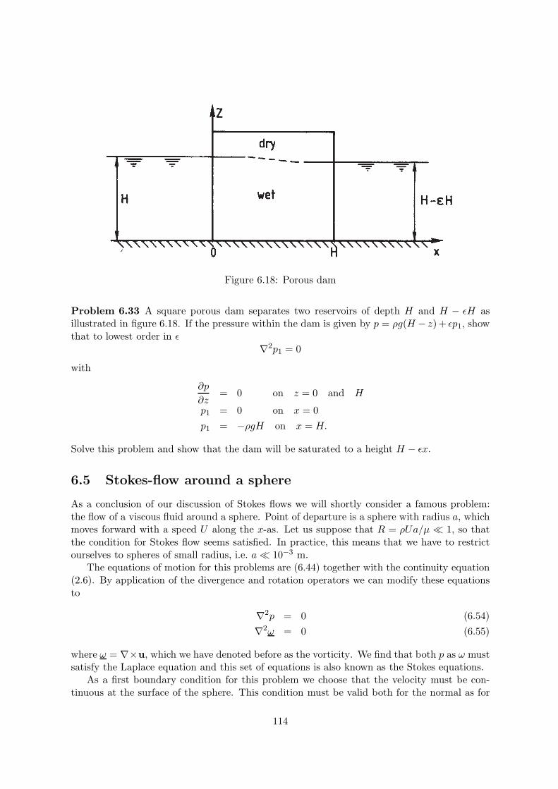
Figure 6.18: Porous dam

Problem 6.33 A square porous dam separates two reservoirs of depth H and H − εH asillustrated in figure 6.18. If the pressure within the dam is given by p = ρg(H − z)+ εp1, showthat to lowest order in ε

∇2p1 = 0

with

∂p

∂z= 0 on z = 0 and H

p1 = 0 on x = 0p1 = −ρgH on x = H.

Solve this problem and show that the dam will be saturated to a height H − εx.

6.5 Stokes-flow around a sphere

As a conclusion of our discussion of Stokes flows we will shortly consider a famous problem:the flow of a viscous fluid around a sphere. Point of departure is a sphere with radius a, whichmoves forward with a speed U along the x-as. Let us suppose that R = ρUa/µ 1, so thatthe condition for Stokes flow seems satisfied. In practice, this means that we have to restrictourselves to spheres of small radius, i.e. a 10−3 m.

The equations of motion for this problems are (6.44) together with the continuity equation(2.6). By application of the divergence and rotation operators we can modify these equationsto

∇2p = 0 (6.54)∇2ω = 0 (6.55)

where ω = ∇×u, which we have denoted before as the vorticity. We find that both p as ω mustsatisfy the Laplace equation and this set of equations is also known as the Stokes equations.

As a first boundary condition for this problem we choose that the velocity must be con-tinuous at the surface of the sphere. This condition must be valid both for the normal as for

114

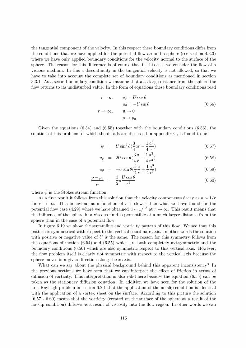
the tangential component of the velocity. In this respect these boundary conditions differ fromthe conditions that we have applied for the potential flow around a sphere (see section 4.3.3)where we have only applied boundary conditions for the velocity normal to the surface of thesphere. The reason for this difference is of course that in this case we consider the flow of aviscous medium. In this a discontinuity in the tangential velocity is not allowed, so that wehave to take into account the complete set of boundary conditions as mentioned in section3.3.1. As a second boundary condition we assume that at a large distance from the sphere theflow returns to its undisturbed value. In the form of equations these boundary conditions read

r = a, ur = U cos θuθ = −U sin θ (6.56)

r → ∞, u → 0p→ p0.

Given the equations (6.54) and (6.55) together with the boundary conditions (6.56), thesolution of this problem, of which the details are discussed in appendix G, is found to be

ψ = U sin2 θ(34ar − 1

4a3

r) (6.57)

ur = 2U cos θ(34a

r− 1

4a3

r3) (6.58)

uθ = −U sin θ(34a

r+

14a3

r3) (6.59)

p− p0

µ=

32aU cos θr2

(6.60)

where ψ is the Stokes stream function.As a first result it follows from this solution that the velocity components decay as u ∼ 1/r

for r → ∞. This behaviour as a function of r is slower than what we have found for thepotential flow case (4.29) where we have obtained u ∼ 1/r3 at r → ∞. This result means thatthe influence of the sphere in a viscous fluid is perceptible at a much larger distance from thesphere than in the case of a potential flow.

In figure 6.19 we show the streamline and vorticity pattern of this flow. We see that thispattern is symmetrical with respect to the vertical coordinate axis. In other words the solutionwith positive or negative value of U is the same. The reason for this symmetry follows fromthe equations of motion (6.54) and (6.55) which are both completely axi-symmetric and theboundary conditions (6.56) which are also symmetric respect to this vertical axis. However,the flow problem itself is clearly not symmetric with respect to the vertical axis because thesphere moves in a given direction along the x-axis.

What can we say about the physical background behind this apparent inconsistency? Inthe previous sections we have seen that we can interpret the effect of friction in terms ofdiffusion of vorticity. This interpretation is also valid here because the equation (6.55) can betaken as the stationary diffusion equation. In addition we have seen for the solution of thefirst Rayleigh problem in section 6.2.1 that the application of the no-slip condition is identicalwith the application of a vortex sheet on the surface. According to this picture the solution(6.57 - 6.60) means that the vorticity (created on the surface of the sphere as a result of theno-slip condition) diffuses as a result of viscosity into the flow region. In other words we can

115

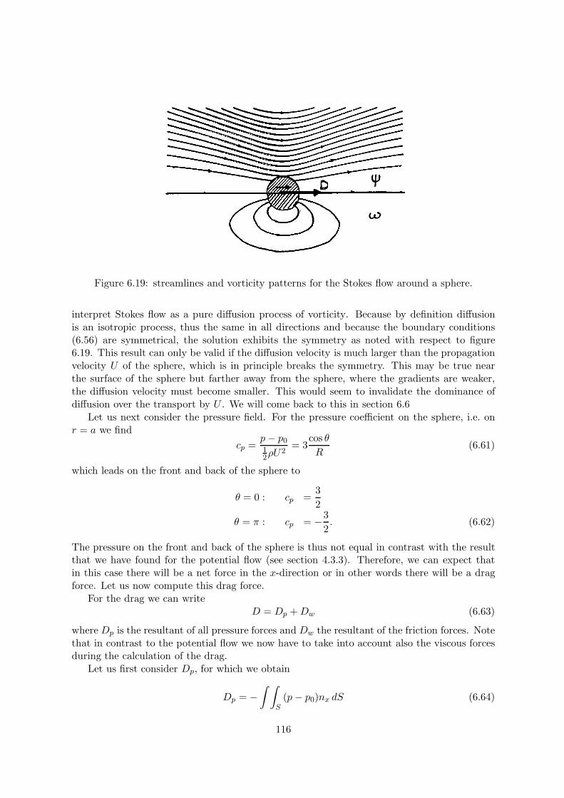
Figure 6.19: streamlines and vorticity patterns for the Stokes flow around a sphere.

interpret Stokes flow as a pure diffusion process of vorticity. Because by definition diffusionis an isotropic process, thus the same in all directions and because the boundary conditions(6.56) are symmetrical, the solution exhibits the symmetry as noted with respect to figure6.19. This result can only be valid if the diffusion velocity is much larger than the propagationvelocity U of the sphere, which is in principle breaks the symmetry. This may be true nearthe surface of the sphere but farther away from the sphere, where the gradients are weaker,the diffusion velocity must become smaller. This would seem to invalidate the dominance ofdiffusion over the transport by U . We will come back to this in section 6.6

Let us next consider the pressure field. For the pressure coefficient on the sphere, i.e. onr = a we find

cp =p− p012ρU

2= 3

cos θR

(6.61)

which leads on the front and back of the sphere to

θ = 0 : cp =32

θ = π : cp = −32. (6.62)

The pressure on the front and back of the sphere is thus not equal in contrast with the resultthat we have found for the potential flow (see section 4.3.3). Therefore, we can expect thatin this case there will be a net force in the x-direction or in other words there will be a dragforce. Let us now compute this drag force.

For the drag we can writeD = Dp +Dw (6.63)

where Dp is the resultant of all pressure forces and Dw the resultant of the friction forces. Notethat in contrast to the potential flow we now have to take into account also the viscous forcesduring the calculation of the drag.

Let us first consider Dp, for which we obtain

Dp = −∫ ∫

S(p − p0)nx dS (6.64)

116

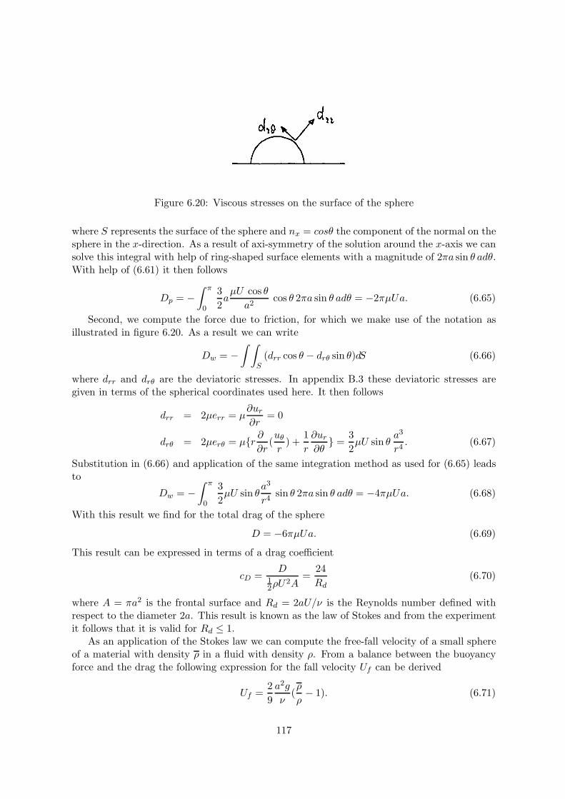
Figure 6.20: Viscous stresses on the surface of the sphere

where S represents the surface of the sphere and nx = cosθ the component of the normal on thesphere in the x-direction. As a result of axi-symmetry of the solution around the x-axis we cansolve this integral with help of ring-shaped surface elements with a magnitude of 2πa sin θ adθ.With help of (6.61) it then follows

Dp = −∫ π

0

32aµU cos θ

a2cos θ 2πa sin θ adθ = −2πµUa. (6.65)

Second, we compute the force due to friction, for which we make use of the notation asillustrated in figure 6.20. As a result we can write

Dw = −∫ ∫

S(drr cos θ − drθ sin θ)dS (6.66)

where drr and drθ are the deviatoric stresses. In appendix B.3 these deviatoric stresses aregiven in terms of the spherical coordinates used here. It then follows

drr = 2µerr = µ∂ur

∂r= 0

drθ = 2µerθ = µr ∂∂r

(uθ

r) +

1r

∂ur

∂θ =

32µU sin θ

a3

r4. (6.67)

Substitution in (6.66) and application of the same integration method as used for (6.65) leadsto

Dw = −∫ π

0

32µU sin θ

a3

r4sin θ 2πa sin θ adθ = −4πµUa. (6.68)

With this result we find for the total drag of the sphere

D = −6πµUa. (6.69)

This result can be expressed in terms of a drag coefficient

cD =D

12ρU

2A=

24Rd

(6.70)

where A = πa2 is the frontal surface and Rd = 2aU/ν is the Reynolds number defined withrespect to the diameter 2a. This result is known as the law of Stokes and from the experimentit follows that it is valid for Rd ≤ 1.

As an application of the Stokes law we can compute the free-fall velocity of a small sphereof a material with density ρ in a fluid with density ρ. From a balance between the buoyancyforce and the drag the following expression for the fall velocity Uf can be derived

Uf =29a2g

ν(ρ

ρ− 1). (6.71)

117

Problem 6.34 A sphere of radius a moves in a straight line through a viscous fluid withvelocity U0 V (t) where V is a non-dimensional function and where t = t′/t0 with t′ time and ta dimensionless time. The Navier-Stokes equations can be non-dimensionalised to

λ∂u∂t

= −∇p+ ∇2u

where λ = a2/(νt0) provided U0a/ν 1. Write down appropriate boundary conditions. Bywriting

u = rot(

0, 0,f(r, t) sin θ

r

)show that f satisfies the equation

frrrr − 4frr

r2+

8fr

r3− 8fr4

= λ

(frrt − 2ft

r2

)

with f(1, t) = V (t)/2, fr(1, t) = V (t) and f → 0 as r → ∞. By taking a Laplace transform int according to

F =∫ ∞

0f e−pt dt = Vg(r)

where

g′′′′ −(

4r2

+ λp

)g′′ +

8r3g′ +

(2λpr2

+8r4

)g = 0.

Given that the solution of this equation, which tends to zero, is r → ∞ is

g =A

r+B

(1r

+√λp

)e−

√λp r

show that

F = V(p)[

12λpr

(3 + 3√λp+ λp) − 3

2λp

(1r

+√λp

)e√

λp (1−r)

].

The non-dimensional drag on the sphere can be shown to be

43π

[−frrr +

4frr

r+fr

r2− 8fr3

+ λfrt

]r=1

.

By evaluating the Laplace transform of this quantity and then inverting, show that the dragbecomes

D = −6πV (t) − 23πλdV (t)dt

− 6√πλ

∫ t

0

dV (s)ds√t− s

ds

Show that this expression leads to the same value for the virtual mass that we have found fora sphere based on potential flow. The last term on the right-hand side of the expression forthe drag is also known as the Basset term.

Problem 6.35 Consider a uniform slow flow past a cylinder and show that the problemreduces to (

∂2

∂r2+

1r

∂

∂r+

1r2∂2

∂θ2

)2

ψ = 0

118

with ∂ψ/∂r = ∂ψ/∂θ = 0 on r = a and

ψ ∼ Ur sin θ as r → ∞.

Show that seeking a solution of the form ψ = f(r) sin θ leads to

ψ =[Ar3 +B r ln r + C r +

D

r

]sin θ

and thus fails because no choice for the integration constant A, B, C and D can be made thatsatisfies all boundary conditions.

It turns out that the expression

ψ =[(r ln r − 1

2r +

12r

)sin θ

]/

[ln(

8R

)− γ +

12

]

with γ = 0.58 the Euler constant satisfies the flow at some distance from the cylinder. Sketchthe streamlines and determine which equation is solved by this solution?

Problem 6.36 A rigid sphere of radius a is immersed in an infinite region of viscous fluid.The sphere rotates with constant angular velocity Ω. The Reynolds number R = Ωa2/ν issmall so that the Stokes equations apply. Using spherical coordinates (r, φ, θ) with θ = 0 alongthe rotation axis, show that a purely rotary flow u = (0, uφ(r, θ), 0) is possible provided that

∂2

∂r2(ruφ) +

1r

∂

∂θ

[1

sin θ∂

∂θ(uφ sin θ)

]= 0.

Write down the boundary conditions, which uφ must satisfy at r = a and as r → ∞. Showthat the appropriate solution to the equation given above, is then given by

uφ =Ωa3

r2sin θ

and show that the torque needed to maintain the rotation of the sphere is

T = 8πµΩa3.

Problem 6.37 Consider the uniform flow past a spherical bubble of radius a by modifyingthe analysis for the Stokes flow around a solid sphere, i.e. by replacing the condition of no-slipby a condition of no tangential stress, i.e. drθ = 0 on r = a. Show in particular that

ψ =12U(r2 − a r

)sin2 θ

and that the normal component of the viscous stress becomes

drr = 3µU

acos θ

and based on this show that the drag on the bubble is

D = 4πµUa.

119

Problem 6.38 Two infinite cylinders of radii a and a′ are rotating with uniform angular ve-locities Ω and Ω′ so as to be always in contact along the z-axis. The cylinders are surroundedby a viscous liquid with viscosity µ and density ρ and the flow can be considered as incom-pressible. Neglecting inertia terms, prove that all the necessary conditions can be satisfied bya stream function of the form

ψ = A sin2 θ +B r2 + C r sin θ +D sin3 θ

r

and determine the integration constants A, B, C and D when the equations of normal sectionsof the cylinders are

r = 2a sin θ, r = 2a′ sin θ.

Examine the case a = a′ and Ω = −Ω′ more particularly, showing that in that case

ψ =12Ωa(r − 4a2 sin3 θ

r

)sin θ.

Compute all the components of the deviatoric stress on the cylinders and discuss the validityof the solution. Compute the torque on the cylinders.

6.6 The Oseen approximation

Let us return to the basic assumption underlying a Stokes flow: i.e. inertia forces are negligiblewith respect to friction forces. We can now check this assumption with help of the exactsolution for the Stokes flow around a sphere.

The magnitude of the viscous forces is estimated with help of the solution (6.58). It thenfollows that ur ∼ Ua/r for r → ∞ so that

µ∇2u µ∂2ur

∂r2∼ µU

a

r3. (6.72)

For the inertia forces we have to take into account that we deal here with an instationaryflow, i.e. the sphere moves through a non-moving fluid. The total acceleration, which is givenhere by the material derivative (1.9) has two contributions: the local derivative ∂u/∂t andthe convective or advective derivative (u.∇)u. The local derivative expresses the fact that thesphere moves in a fixed coordinate system that is attached to the quiescent fluid, in which thesphere is moving. After all when we take a coordinate system fixed to the sphere, this localderivative disappears because in such a coordinate system the flow is stationary. This impliesthat we can estimate ∂u/∂t based on a translation transformation which means that for thisterm we can write

ρ∂u∂t

ρ(U.∇)u ρU∂ur

∂x∼ ρU2 a

r2. (6.73)

For the non-linear advective or convective term follows

ρ(u.∇)u ρur∂ur

∂r∼ ρU2 a

2

r3. (6.74)

For both the estimates (6.73) and (6.74) we can determine the ratio of the inertia versusthe friction forces. The result reads

ρ∂u/∂tµ∇2u

Rdr

a(6.75)

ρ(u · ∇)uµ∇2u

Rd. (6.76)

120

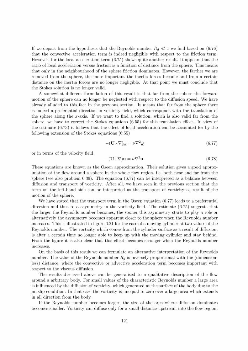
If we depart from the hypothesis that the Reynolds number Rd 1 we find based on (6.76)that the convective acceleration term is indeed negligible with respect to the friction term.However, for the local acceleration term (6.75) shows quite another result. It appears that theratio of local acceleration versus friction is a function of distance from the sphere. This meansthat only in the neighbourhood of the sphere friction dominates. However, the farther we areremoved from the sphere, the more important the inertia forces become and from a certaindistance on the inertia forces are no longer negligible. At that point we must conclude thatthe Stokes solution is no longer valid.

A somewhat different formulation of this result is that far from the sphere the forwardmotion of the sphere can no longer be neglected with respect to the diffusion speed. We havealready alluded to this fact in the previous section. It means that far from the sphere thereis indeed a preferential direction in vorticity field, which corresponds with the translation ofthe sphere along the x-axis. If we want to find a solution, which is also valid far from thesphere, we have to correct the Stokes equations (6.55) for this translation effect. In view ofthe estimate (6.73) it follows that the effect of local acceleration can be accounted for by thefollowing extension of the Stokes equations (6.55)

−(U · ∇)ω = ν∇2ω (6.77)

or in terms of the velocity field−(U · ∇)u = ν∇2u. (6.78)

These equations are known as the Oseen approximation. Their solution gives a good approx-imation of the flow around a sphere in the whole flow region, i.e. both near and far from thesphere (see also problem 6.39). The equation (6.77) can be interpreted as a balance betweendiffusion and transport of vorticity. After all, we have seen in the previous section that theterm on the left-hand side can be interpreted as the transport of vorticity as result of themotion of the sphere.

We have stated that the transport term in the Oseen equation (6.77) leads to a preferentialdirection and thus to a asymmetry in the vorticity field. The estimate (6.75) suggests thatthe larger the Reynolds number becomes, the sooner this asymmetry starts to play a role oralternatively the asymmetry becomes apparent closer to the sphere when the Reynolds numberincreases. This is illustrated in figure 6.21 for the case of a moving cylinder at two values of theReynolds number. The vorticity which comes from the cylinder surface as a result of diffusion,is after a certain time no longer able to keep up with the moving cylinder and stay behind.From the figure it is also clear that this effect becomes stronger when the Reynolds numberincreases.

On the basis of this result we can formulate an alternative interpretation of the Reynoldsnumber. The value of the Reynolds number Rd is inversely proportional with the (dimension-less) distance, where the convective or advective acceleration term becomes important withrespect to the viscous diffusion.

The results discussed above can be generalised to a qualitative description of the flowaround a arbitrary body. For small values of the characteristic Reynolds number a large areais influenced by the diffusion of vorticity, which generated at the surface of the body due to theno-slip condition. In that case the vorticity is unequal to zero over a large area which extendsin all direction from the body.

If the Reynolds number becomes larger, the size of the area where diffusion dominatesbecomes smaller. Vorticity can diffuse only for a small distance upstream into the flow region,

121

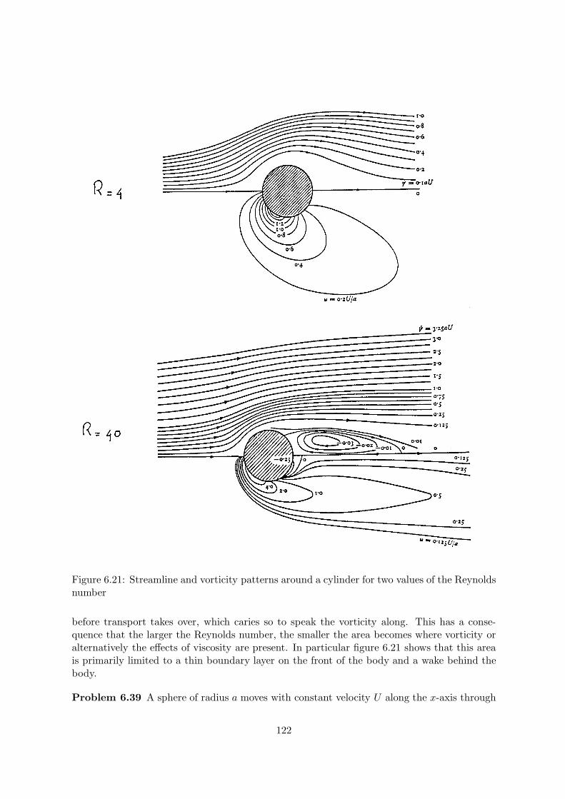
Figure 6.21: Streamline and vorticity patterns around a cylinder for two values of the Reynoldsnumber

before transport takes over, which caries so to speak the vorticity along. This has a conse-quence that the larger the Reynolds number, the smaller the area becomes where vorticity oralternatively the effects of viscosity are present. In particular figure 6.21 shows that this areais primarily limited to a thin boundary layer on the front of the body and a wake behind thebody.

Problem 6.39 A sphere of radius a moves with constant velocity U along the x-axis through

122

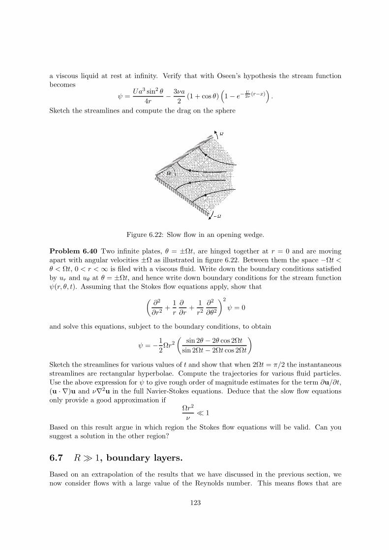
a viscous liquid at rest at infinity. Verify that with Oseen’s hypothesis the stream functionbecomes

ψ =Ua3 sin2 θ

4r− 3νa

2(1 + cos θ)

(1 − e−

U2ν

(r−x)).

Sketch the streamlines and compute the drag on the sphere

Figure 6.22: Slow flow in an opening wedge.

Problem 6.40 Two infinite plates, θ = ±Ωt, are hinged together at r = 0 and are movingapart with angular velocities ±Ω as illustrated in figure 6.22. Between them the space −Ωt <θ < Ωt, 0 < r < ∞ is filed with a viscous fluid. Write down the boundary conditions satisfiedby ur and uθ at θ = ±Ωt, and hence write down boundary conditions for the stream functionψ(r, θ, t). Assuming that the Stokes flow equations apply, show that

(∂2

∂r2+

1r

∂

∂r+

1r2

∂2

∂θ2

)2

ψ = 0

and solve this equations, subject to the boundary conditions, to obtain

ψ = −12Ωr2

(sin 2θ − 2θ cos 2Ωt

sin 2Ωt− 2Ωt cos 2Ωt

)

Sketch the streamlines for various values of t and show that when 2Ωt = π/2 the instantaneousstreamlines are rectangular hyperbolae. Compute the trajectories for various fluid particles.Use the above expression for ψ to give rough order of magnitude estimates for the term ∂u/∂t,(u · ∇)u and ν∇2u in the full Navier-Stokes equations. Deduce that the slow flow equationsonly provide a good approximation if

Ωr2

ν 1

Based on this result argue in which region the Stokes flow equations will be valid. Can yousuggest a solution in the other region?

6.7 R 1, boundary layers.

Based on an extrapolation of the results that we have discussed in the previous section, wenow consider flows with a large value of the Reynolds number. This means flows that are

123

dominated by inertia. We have seen that R → ∞ does not mean that viscous effects can betotally neglected. It means that the influence of viscosity becomes limited to an increasinglysmaller region. Nevertheless, we always need viscosity to satisfy the no-slip condition. Theflow of any real fluid, which satisfies the Navier-Stokes equations, differs in this respect thusessentially from the case of the ideal fluids, which satisfy the Euler equations. In other wordsthe limit R → ∞ in the solution of the Navier-Stokes equations is different from carrying outthis limit in the Navier-Stokes equations themselves. Such a limit is called singular. We havealready referred to the importance of viscosity in satisfying the no-slip boundary condition insections 3.3.1 and 4.1, where we discussed the boundary conditions.

We have said that the limit R→ ∞ one could expect that the region of influence of viscosityapproaches to zero. As soon as vorticity is created by the no-slip condition, it is carried along bytransport. This is indeed the case for special geometries, which we call streamlined. Examplesare a flat plat where the velocity is parallel to the plate or an airfoil. The small region nearthe body, to which in that case the influence of viscosity is limited, is called a boundary layer.We shall come back to the boundary layer in more detail in section 6.7.1.

For non-streamlined bodies the situation becomes somewhat more complex and this isfor instance illustrated by the cylinder flow in figure 6.21. For large values of the Reynoldsnumber a boundary layer develops on the front of the cylinder. However, by the dominanceof the convection or advection term the vorticity (created at the surface of the cylinder) istransported backwards to the rear of the cylinder where a region of concentrated vorticity iscreated. Such an region behind a non-streamlined or alternatively a bluff body is called aseparation region because an alternative way of explaining this region is through separationof the boundary layer from the body as a result of an adverse pressure gradient outside theboundary layer as will be discussed further in section 6.7.1.

We find thus that for a streamlined body the flow in the limit R → ∞ approaches moreand more the flow field that would result from the inviscid Euler equations apart from a verythin boundary layer close to the surface of the body. In contrast for a non-streamlined bodyeven in the R→ ∞ a wake or separation region remains present (although the exact form andcharacteristics of such region at R = ∞ is not known). The flow field will be any case differentfrom the solution of the Euler equations. Take for instance the flow around a cylinder. Thesolution of the Euler equations for a cylinder flow has been discussed in section 4.4.1 and itis clear that the solution of the Navier-Stokes equations as e.g. shown in figure 6.21 is quitedifferent. As mentioned already this may seem a contradiction because the Euler equationscan be obtained from the Navier-Stokes equations by taking the limit R → ∞. However, weshould remember that by taking the limit in the Navier-Stokes equations we reduce the orderof the differential equations and as a result we reduce the number of boundary conditions thatwe can take into account. In other words by taking the limit R → ∞ in the Navier-Stokesequations we change the type of the equations. As already mentioned such a limit process iscalled singular.

6.7.1 Boundary layers near a flat plate

Let us return to flows, which are characterized by a large Reynolds number. Let us repeat thecharacteristic properties, which we have discussed for this type of flow in section 6.6. As anexample we take the flow geometry which is sketched in figure 6.23, which shows a flow parallelto a flat plate. The following aspects can be recognized

124

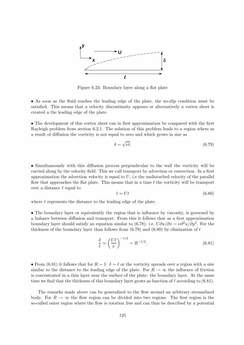
Uy

x

δ

Figure 6.23: Boundary layer along a flat plate

• As soon as the fluid reaches the leading edge of the plate, the no-slip condition must besatisfied. This means that a velocity discontinuity appears or alternatively a vortex sheet iscreated a the leading edge of the plate.

• The development of this vortex sheet can in first approximation be compared with the firstRayleigh problem from section 6.2.1. The solution of this problem leads to a region where asa result of diffusion the vorticity is not equal to zero and which grows in size as

δ ∼ √νt. (6.79)

• Simultaneously with this diffusion process perpendicular to the wall the vorticity will becarried along by the velocity field. This we call transport by advection or convection. In a firstapproximation the advection velocity is equal to U , i.e the undisturbed velocity of the parallelflow that approaches the flat plate. This means that in a time t the vorticity will be transportover a distance equal to

= Ut (6.80)

where represents the distance to the leading edge of the plate.

• The boundary layer or equivalently the region that is influence by viscosity, is governed bya balance between diffusion and transport. From this it follows that as a first approximationboundary layer should satisfy an equation similar to (6.78): i.e. U∂u/∂x = ν∂2u/∂y2. For thethickness of the boundary layer than follows from (6.79) and (6.80) by elimination of t

δ

(U

ν

)−1/2

= R−1/2. (6.81)

• From (6.81) it follows that for R ∼ 1: δ ∼ or the vorticity spreads over a region with a sizesimilar to the distance to the leading edge of the plate. For R → ∞ the influence of frictionis concentrated in a thin layer near the surface of the plate: the boundary layer. At the sametime we find that the thickness of this boundary layer grows as function of according to (6.81).

The remarks made above can be generalised to the flow around an arbitrary streamlinedbody. For R → ∞ the flow region can be divided into two regions. The first region is theso-called outer region where the flow is rotation free and can thus be described by a potential

125

flow. The second region is the boundary layer, also called inner region, where the flow isinfluenced by viscosity in order to satisfy the no-slip condition on the surface of the body.

In the remaining of this section we go into somewhat more details in the case of a stationaryflow geometry near a flat plate and we shall see how we can quantify the general characteristicsof the boundary layer. We shall distinguish two cases:

1. undisturbed velocity perpendicular to the plate.2. undisturbed velocity parallel to the plate.

Case 1: undisturbed velocity perpendicular to the plate

As illustration for this type of flow we may take a flat plate with suction or the stagnation pointflow. In both cases there is a velocity component in the direction of the wall or in other words avelocity component opposite to the diffusion velocity of the vorticity from the wall. The resultis that the region where vorticity is present has a constant thickness which is determined bythe balance between the two velocities, i.e. a balance between transport and diffusion.

Let us consider the flat plate with suction in somewhat more detail. Consider a stationary,two-dimensional flow over a infinite flat plate at y = 0, i.e. along the x-axis. The followingboundary conditions should be satisfied

y = 0, u = 0, v = −V (6.82)y → ∞, u→ U

where U is the undisturbed velocity parallel to the plate. In view of the fact that the plateis infinite for x → ±∞ we suppose that the flow is independent of the x-coordinate. Fromthe continuity equation it follows then that the velocity component perpendicular on the plateshould be independent of the y-coordinate and thus constant. From the boundary conditions itthen follows that v = −V . With this result the equation of motion for this flow field becomes

−V ∂u∂y

= ν∂2u

∂y2. (6.83)

The solution of this equation, which satisfies the boundary conditions, reads

u = U

[1 − exp

(− V y

ν

)]. (6.84)

From this it follows that the thickness of the layer, in which the velocity components u adjuststo the boundary condition at the wall, is equal to δ ∼ ν/V . For the further details of thestagnation point flow we refer to section 5.5 of Batchelor.

Case 2: undisturbed velocity parallel to the plate

The second case concerns the flow geometry, in which there is an undisturbed velocity Uparallel to the plate. On the plate the no-slip condition should be satisfied and at the sametime the normal velocity component v should be zero. In that case the transport of vorticityby the x-component of the velocity is perpendicular to the diffusion direction. The plate issemi-infinite and starts at x = 0 and we consider again a two-dimensional flow geometry. From(6.81) we know that the thickness of the boundary layer δ should be small with respect to the

126

distance to the leading edge of the plate, which is , i.e. δ/ 1. We shall make use of thisresult to estimate the magnitude in the various terms in the equations of motion.

The complete Navier-Stokes equations for the case of a two-dimensional, incompressibleand stationary flow read

∂u

∂x+∂v

∂y= 0 (6.85)

u∂u

∂x+ v

∂u

∂y= −1

ρ

∂p

∂x+ ν

(∂2u

∂x2+∂2u

∂y2

)(6.86)

u∂v

∂x+ v

∂v

∂y= −1

ρ

∂p

∂y+ ν

(∂2v

∂x2+∂2v

∂y2

)(6.87)

For a characteristic length scale perpendicular to the plate we take δ whereas for the lengthscale along the direction of the plate we take . For the velocity scale we shall take U . Thefollowing order-of-magnitude estimates can be made

∂

∂x∼ 1

(6.88)

∂

∂y∼ 1δ

(6.89)

u ∼ U. (6.90)

Application of these scaling estimates in the continuity equation (6.85) leads to an order-of-magnitude estimate for v, i.e. the y-component of the velocity. The result reads

v ∼ δ

U. (6.91)

Subsequently we apply the scaling estimates (6.88 - 6.91) to the equations (6.86) and (6.87).An example is ∂2u/∂x2 ∼ U/2 and ∂2u/∂y2 ∼ U/δ2. Next we make use of (6.81). For R→ ∞it then follows that ∂2u/∂x2 is negligible with respect to ∂2u/∂y2. Application of the scalingrules to the other terms then leads to the following equations

∂u

∂x+∂v

∂y= 0

u∂u

∂x+ v

∂u

∂y= −1

ρ

∂p

∂x+ ν

∂2u

∂y2(6.92)

∂p

∂y= 0, (6.93)

which are known as Prandtl’s boundary-layer equations.We thus find that the diffusion component in the x-direction is negligible with respect to

the diffusion component in the y-direction. At the same time it follows that pressure gradientacross the boundary layer can be neglected. This means that the pressure in the boundarylayer is equal to the pressure outside the boundary layer, i.e. in the rotation free outer layer,which, as we have argued before, can be described in terms of potential flow theory. Thismeans that the pressure can be computed with help of the law of Bernouilli (4.7) so that

−1ρ

∂p

∂x= U

dU

dx. (6.94)

127

With help of this result the momentum equation (6.92) can be written as

u∂u

∂x+ v

∂u

∂y= U

dU

dx+ ν

∂2u

∂y2. (6.95)

This equation has been derived by Prandtl in 1905.The boundary conditions, which must be satisfied by the solution of (6.95), read

y = 0, u = 0, v = 0 (6.96)y → ∞, u→ U.

The equations (6.85) and (6.95) together with the boundary conditions (6.96) form a closedsystem. Let us now consider the flow geometry for a flat plat with U = constant.

Because the flow is two dimensional. we can make use of the stream function ψ, which isdefined according to (2.8). With this stream function we integrate the continuity equation.Let us now look for the following similarity solution

ψ = Uδ f(y

δ). (6.97)

Here, δ = δ(x), which is the boundary-layer thickness, is taken as the characteristic scale ofthe flow in the y-direction. With this definition of ψ (2.8) we then find

u = Udf

dη(6.98)

v = −U dδdx

(f − ηdf

dη) (6.99)

where η = y/δ. Next we substitute these velocity components in (6.95) with as result

d3f

dη3+Uδ

ν

dδ

dxfd2f

dη2= 0. (6.100)

The condition for the existence of a similarity solution is that the coefficients in (6.100) shouldbe not a function of x and this implies

Uδ

ν

dδ

dx= constant. (6.101)

Let us for the constant take the value 1/2. The solution of (6.101) then reads

δ =√νx

U(6.102)

where we have used the boundary condition that at the leading edge of the plat, i.e. x = 0, theboundary-layer thickness is zero. With this result the equation for the boundary layer becomes

d3f

dη3+

12fd2f

dη2= 0 (6.103)

which is known as the Blasius equation.

128

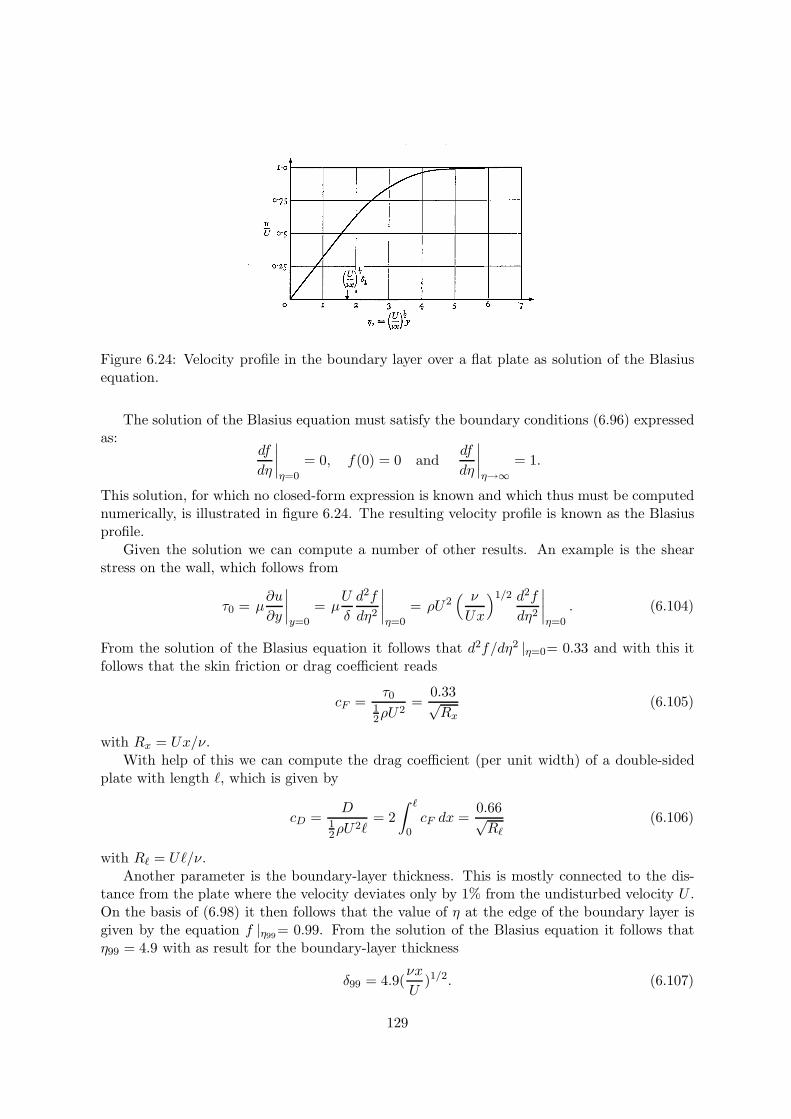
Figure 6.24: Velocity profile in the boundary layer over a flat plate as solution of the Blasiusequation.

The solution of the Blasius equation must satisfy the boundary conditions (6.96) expressedas:

df

dη

∣∣∣∣η=0

= 0, f(0) = 0 anddf

dη

∣∣∣∣η→∞

= 1.

This solution, for which no closed-form expression is known and which thus must be computednumerically, is illustrated in figure 6.24. The resulting velocity profile is known as the Blasiusprofile.

Given the solution we can compute a number of other results. An example is the shearstress on the wall, which follows from

τ0 = µ∂u

∂y

∣∣∣∣y=0

= µU

δ

d2f

dη2

∣∣∣∣η=0

= ρU2( ν

Ux

)1/2 d2f

dη2

∣∣∣∣η=0

. (6.104)

From the solution of the Blasius equation it follows that d2f/dη2 |η=0= 0.33 and with this itfollows that the skin friction or drag coefficient reads

cF =τ0

12ρU

2=

0.33√Rx

(6.105)

with Rx = Ux/ν.With help of this we can compute the drag coefficient (per unit width) of a double-sided

plate with length , which is given by

cD =D

12ρU

2= 2

∫

0cF dx =

0.66√R

(6.106)

with R = U/ν.Another parameter is the boundary-layer thickness. This is mostly connected to the dis-

tance from the plate where the velocity deviates only by 1% from the undisturbed velocity U .On the basis of (6.98) it then follows that the value of η at the edge of the boundary layer isgiven by the equation f |η99= 0.99. From the solution of the Blasius equation it follows thatη99 = 4.9 with as result for the boundary-layer thickness

δ99 = 4.9(νx

U)1/2. (6.107)

129

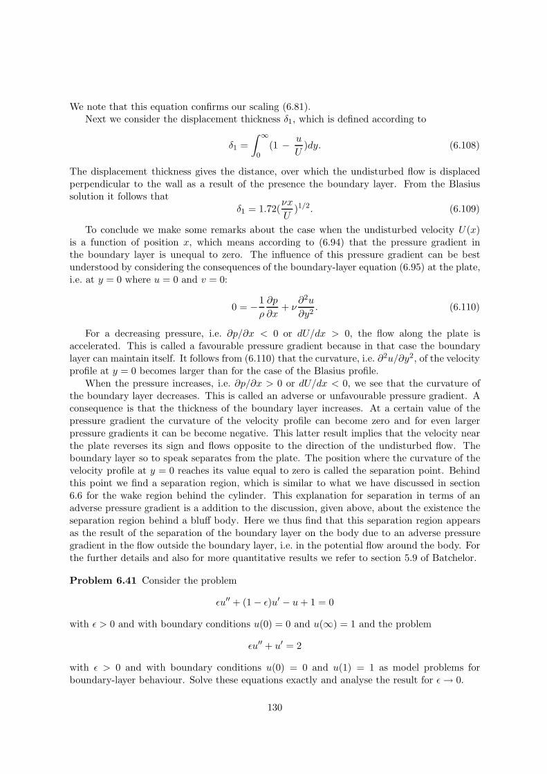
We note that this equation confirms our scaling (6.81).Next we consider the displacement thickness δ1, which is defined according to

δ1 =∫ ∞

0(1 − u

U)dy. (6.108)

The displacement thickness gives the distance, over which the undisturbed flow is displacedperpendicular to the wall as a result of the presence the boundary layer. From the Blasiussolution it follows that

δ1 = 1.72(νx

U)1/2. (6.109)

To conclude we make some remarks about the case when the undisturbed velocity U(x)is a function of position x, which means according to (6.94) that the pressure gradient inthe boundary layer is unequal to zero. The influence of this pressure gradient can be bestunderstood by considering the consequences of the boundary-layer equation (6.95) at the plate,i.e. at y = 0 where u = 0 and v = 0:

0 = −1ρ

∂p

∂x+ ν

∂2u

∂y2. (6.110)

For a decreasing pressure, i.e. ∂p/∂x < 0 or dU/dx > 0, the flow along the plate isaccelerated. This is called a favourable pressure gradient because in that case the boundarylayer can maintain itself. It follows from (6.110) that the curvature, i.e. ∂2u/∂y2, of the velocityprofile at y = 0 becomes larger than for the case of the Blasius profile.

When the pressure increases, i.e. ∂p/∂x > 0 or dU/dx < 0, we see that the curvature ofthe boundary layer decreases. This is called an adverse or unfavourable pressure gradient. Aconsequence is that the thickness of the boundary layer increases. At a certain value of thepressure gradient the curvature of the velocity profile can become zero and for even largerpressure gradients it can be become negative. This latter result implies that the velocity nearthe plate reverses its sign and flows opposite to the direction of the undisturbed flow. Theboundary layer so to speak separates from the plate. The position where the curvature of thevelocity profile at y = 0 reaches its value equal to zero is called the separation point. Behindthis point we find a separation region, which is similar to what we have discussed in section6.6 for the wake region behind the cylinder. This explanation for separation in terms of anadverse pressure gradient is a addition to the discussion, given above, about the existence theseparation region behind a bluff body. Here we thus find that this separation region appearsas the result of the separation of the boundary layer on the body due to an adverse pressuregradient in the flow outside the boundary layer, i.e. in the potential flow around the body. Forthe further details and also for more quantitative results we refer to section 5.9 of Batchelor.

Problem 6.41 Consider the problem

εu′′ + (1 − ε)u′ − u+ 1 = 0

with ε > 0 and with boundary conditions u(0) = 0 and u(∞) = 1 and the problem

εu′′ + u′ = 2

with ε > 0 and with boundary conditions u(0) = 0 and u(1) = 1 as model problems forboundary-layer behaviour. Solve these equations exactly and analyse the result for ε→ 0.

130

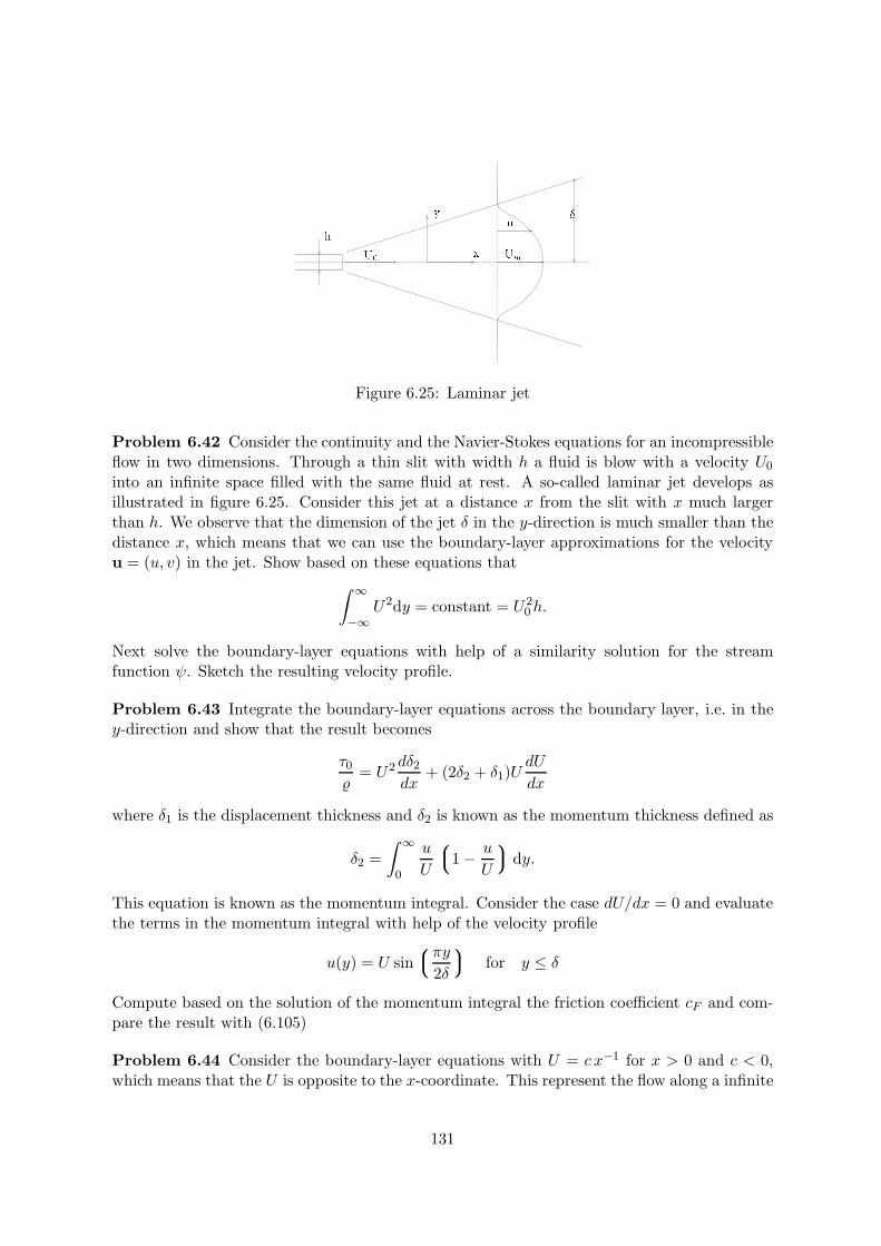
y

hu

xU Um

Figure 6.25: Laminar jet

Problem 6.42 Consider the continuity and the Navier-Stokes equations for an incompressibleflow in two dimensions. Through a thin slit with width h a fluid is blow with a velocity U0

into an infinite space filled with the same fluid at rest. A so-called laminar jet develops asillustrated in figure 6.25. Consider this jet at a distance x from the slit with x much largerthan h. We observe that the dimension of the jet δ in the y-direction is much smaller than thedistance x, which means that we can use the boundary-layer approximations for the velocityu = (u, v) in the jet. Show based on these equations that∫ ∞

−∞U2dy = constant = U2

0h.

Next solve the boundary-layer equations with help of a similarity solution for the streamfunction ψ. Sketch the resulting velocity profile.

Problem 6.43 Integrate the boundary-layer equations across the boundary layer, i.e. in they-direction and show that the result becomes

τ0

= U2 dδ2dx

+ (2δ2 + δ1)UdU

dx

where δ1 is the displacement thickness and δ2 is known as the momentum thickness defined as

δ2 =∫ ∞

0

u

U

1 − u

U

dy.

This equation is known as the momentum integral. Consider the case dU/dx = 0 and evaluatethe terms in the momentum integral with help of the velocity profile

u(y) = U sinπy

2δ

for y ≤ δ

Compute based on the solution of the momentum integral the friction coefficient cF and com-pare the result with (6.105)

Problem 6.44 Consider the boundary-layer equations with U = c x−1 for x > 0 and c < 0,which means that the U is opposite to the x-coordinate. This represent the flow along a infinite

131

plate into a two-dimensional sink. Look for a similarity solution of the stream function of thefollowing form

ψ = (νUx)1/2f(η) with η = U/(νx)1/2y.

Solve the resulting ordinary differential equation and discuss the result. Is there a solution forc > 0?

Problem 6.45 Consider the solution (4.42) for the potential flow around a cylinder in aparallel flow with velocity U0 (in the negative x-direction). For the case of a real fluid aboundary layer develops due to the no-slip condition on the front of the cylinder starting atthe stagnation point θ = 0. The boundary-layer equations for the velocity component uθ areapproximated as

Uθduθ

ds= −1

dp

ds+ ν

∂2uθ

∂n2

where s is the coordinate along and n the coordinate perpendicular to the surface of thecylinder. De Uθ ≡ Uθ(r = a) is the tangential component at r = a of the potential flow outsidethe cylinder. The pressure gradient dp/ds may be written as

−1

dp

ds= Uθ

dUθ

ds.

Formulate the equivalent momentum integral for this case as considered in problem 6.43.Assume that the velocity profile in the boundary-layer can be approximated with

uθ = c1n+ c2n2 + c3n

3

where the c1, c2 and c3 are constants, which can be determined with help of the boundaryconditions for the velocity. Evaluate the constants in the momentum integral and solve theresulting equation as a function of s. Compute the friction coefficient cF as a function of s anddetermine where the separation point occurs. Based on this result compute the friction dragof the sphere and compare this with the total drag coefficient, which is given by

cD =D

12ρU0A

1

where A is the frontal area (per unit width) of the cylinder.

Problem 6.46 Consider the boundary layer above a flat surface in a Cartesian rotating co-ordinate system. Assume that the velocity profile is only a function of the vertical coordinatez such that u = (u(z), v(z), 0) which satisfies the continuity equation. Show that the resultingequations become

−fv = −1ρ

∂p

∂x+ ν

∂2u

∂z2

fu = −1ρ

∂p

∂y+ ν

∂2v

∂z2,

where the pressure gradients, ∂p/∂x and ∂p/∂y, which do not depend on z, are assumed asgiven. Far from the surface the flow must satisfy the inviscid equations

−fv = −1ρ

∂p

∂x

fu = −1ρ

∂p

∂y,

132

which is called the geostrophic balance. Solve the equations for the boundary layer betweenthe surface and the inviscid solution. This layer is generally known as the Ekman layer.

Problem 6.47 Consider a general similarity solution for a two-dimensional boundary-layerflow given by the following stream function

ψ = F (x)f(

y

g(x)

)

Show that the equations demand that

F (x) = U(x)g(x)

and that the resulting similarity equation becomes

f ′2 −

(1 +

Ug′

U ′g

)f f ′′ = 1 +

ν

U ′g2f ′′′

where a prime denotes a differentiation with respect to η = y/g(x). Deduce that similaritysolutions are only possible when

either U ∝ (x− x0)m or U ∝ eα x

where x0, m and α are constants.Show in the case U = Axm with A > 0 that the g(x) can be chosen as

g(x) =[

2 ν(m+ 1)Axm+1

] 12

and that equation for f(x) in that case becomes

f ′′′ + f f ′′ +2mm+ 1

(1 − f ′

2)

with the boundary conditions

f(0) = f ′′(0) = 0 and f ′(∞) = 1.

This is known as the Falkner-Skan equation. Solve the equation for m = 1 exactly and showthat this represents the boundary-layer development in the neighbourhood of a two-dimensionalstagnation point Consider the solution of this equation for a general value of m with help ofnumerical methods. Show that for m > 0 there is always a solution with u > 0 everywhere.Show that for m < 0 a solution for u > 0 everywhere is only possible for m > −0.0904.Interpret these results in terms of the effect of the pressure gradient on the boundary layer.Compare also with problems 6.44 and 4.22.

Problem 6.48 At a large distance x downstream of a body in a two-dimensional parallel flowU of a viscous fluid we observe a wake with a velocity profile u(x, y). Prove that the drag Dof the body (per unit width) follows from

D = ρ

∫ ∞

−∞u(U − u) dy.

133

The wake has a transverse dimension δ in the y-direction. Assume that δ x so that theboundary-layer approximations can be used. Furthermore, we assume the velocity profile tobe given by

u(x, y) = U − ucl(x)f (η)

with η = y/δ(x) and ucl the velocity on the centreline of the wake and ucl U so that theexpression for the drag derived above can be simplified to

D = ρucl(x)U∫ ∞

−∞f

(y

δ(x)

)dy

Derive a similarity equation for f(η) and an expression for the δ as function of x. Solve theresulting equation for f .

Problem 6.49 Solve the equivalent problem 6.42 for the laminar jet and 6.48 for laminarwake but now in three dimensions. for which we can assume an axisymmetric flow.

134

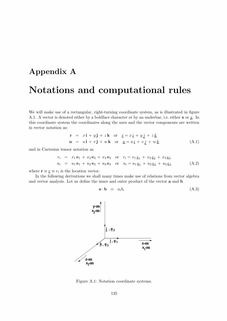
Appendix A

Notations and computational rules

We will make use of a rectangular, right-turning coordinate system, as is illustrated in figureA.1. A vector is denoted either by a boldface character or by an underbar, i.e. either x or x. Inthis coordinate system the coordinates along the axes and the vector components are writtenin vector notation as:

r = x i + y j + z k or r = x i + y j + z k

u = u i + v j + w k or u = u i + v j + w k (A.1)

and in Cartesian tensor notation as

ri = x1 e1 + x2 e2 + x3 e3 or ri = x1 e1 + x2 e2 + x3 e3

ui = u1 e1 + u2 e2 + u3 e3 or ui = u1 e1 + u2 e2 + u3 e3 (A.2)

where r ≡ r ≡ ri is the location vector.In the following derivations we shall many times make use of relations from vector algebra

and vector analysis. Let us define the inner and outer product of the vector a and b

a · b ≡ aibi (A.3)

y-asx -as

x-asx -as

z-asx -as

j , e

i , ek , e

1

2

3

1

2

3

Figure A.1: Notation coordinate systems.

135

a × b ≡ εijkajbk (A.4)

where the εijk represents the permutation tensor, i.e.: εijk = 0 when two or more indices havethe same value and εijk = 1 when the indices have a cyclic permutation, i.e. ε123 = ε231 =ε312 = 1 and εijk = −1 for an anticyclic permutation, i.e. ε213 = ε132 = ε321 = −1. Animportant relationship for the permutation tensor, which we shall use several times, reads

εimjεikl = δmkδjl − δmlδjk. (A.5)

where δij the Kronecker delta is, for which δij = 1 when i = j and δij = 0 when i = jLet us now introduce the gradient, the divergence and the rotation operator.

∇Φ ≡ grad Φ ≡ ∂Φ∂xi

(A.6)

∇ · u ≡ divu ≡ ∂ui

∂xi(A.7)

∇× u ≡ rotu ≡ εijk∂uk

∂xj. (A.8)

where ∇ is sometimes called the nabla operator. The gradient operator, grad, represents thegradient of a scalar function Φ in the direction of the normal on the surface Φ = constant.A physical interpretation of the divergence operator, div, and the rotation operator, rot, arediscussed in section 2.1 and 2.3.2, respectively.

Finally we present some integral relationships. First the divergence theorem of Gauss:∫ ∫ ∫V

divu dV =∫ ∫

Su · n dS (A.9)∫ ∫ ∫

V

∂ui

∂xidV =

∫ ∫Suini dS (A.10)

where V represents a volume with a surface S and n ≡ ni is the normal on the surface S,which is directed positive outwards.

Second the theorem of Stokes:∫ ∫A

n · rotu dS =∮

u · ds (A.11)∫ ∫Ani εijk

∂uk

∂xjdS =

∮ui dsi (A.12)

where A represents a surface with a edge S. The direction of the normal n ≡ ni on A satisfiesa right-hand turning cork-screw rule for the direction of integration along S.

Given the definitions which we have introduces above, we are able to derive a number ofrelationships, of which we give here some examples (without proof) and which we shall use atvarious places in the text

a × (b× c) = (a · c)b − (a · b)c (A.13)∇× (∇Φ) = 0 (A.14)

∇ · (∇× u) = 0 (A.15)

(u · ∇)u =12∇(u · u) − u × (∇× u) (A.16)

136

∇ · (Φu) = Φ∇ · u + (u · ∇)Φ (A.17)∇× (Φu) = Φ × (∇× u) + grad Φ × u (A.18)

∇× (∇× u) = ∇(∇ · u) − (∇ · ∇)u (A.19)∇ · (u × ω) = ω · (∇× u) − u · (∇× ω) (A.20)

∇× (u × ω) = (ω · ∇)u− ω(∇u) − (u · ∇)ω + u(∇ · ω) (A.21)∇(u · ω) = (ω · ∇)u + (u · ∇)ω +

ω × (∇× u) + u × (∇× ω) (A.22)

137

Appendix B

Curvilinear coordinates.

B.1 Theory

The definition of the material derivative (1.6) and (1.7) is in principle valid for the change ofa flow or fluid property along the trajectory of a fluid element. Application of (1.6) to thevelocity u(x, t) leads to the expression

DuDt

=∂u∂t

+ (u · grad)u (B.1)

which gives the acceleration of a fluid element in a Eulerian coordinate system. In Cartesiantensor notation (B.1) reduces to

Dui

Dt=∂ui

∂t+ uj

∂ui

∂xj. (B.2)

We stress here that the expression (B.2) is only valid in a Cartesian coordinate system. In ageneral curvilinear coordinate system we will find some additional terms known as the curvatureterms. These terms are the consequence of the fact that in a curvilinear coordinate systemthe direction of the unit vectors are a function of position. Here we shall briefly discuss theformulation of several vector quantities in a general, rectangular, curvilinear coordinate system(rectangular means that at each point in space the coordinate directions are perpendicular toeach other).

Consider the transformation

ξ1 = ξ1(x1, x2, x3)ξ2 = ξ2(x1, x2, x3) (B.3)ξ3 = ξ3(x1, x2, x3).

Let us suppose that this transformation is reversible so that we can also write

x1 = x1(ξ1, ξ2, ξ3)x2 = x2(ξ1, ξ2, ξ3) (B.4)x3 = x3(ξ1, ξ2, ξ3).

138

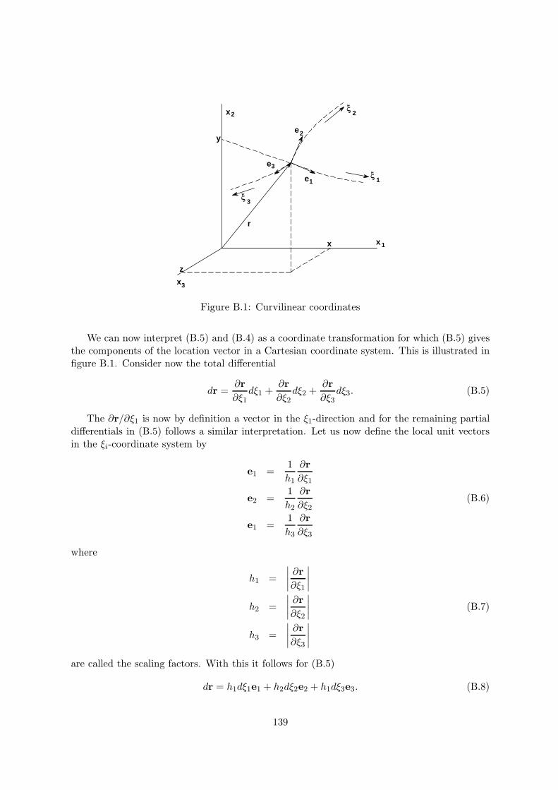
ξ

ξ

ξ

1

2

3

1

2

3

1

2

3

x

x

x

e

e

e

r

x

y

z

Figure B.1: Curvilinear coordinates

We can now interpret (B.5) and (B.4) as a coordinate transformation for which (B.5) givesthe components of the location vector in a Cartesian coordinate system. This is illustrated infigure B.1. Consider now the total differential

dr =∂r∂ξ1

dξ1 +∂r∂ξ2

dξ2 +∂r∂ξ3

dξ3. (B.5)

The ∂r/∂ξ1 is now by definition a vector in the ξ1-direction and for the remaining partialdifferentials in (B.5) follows a similar interpretation. Let us now define the local unit vectorsin the ξi-coordinate system by

e1 =1h1

∂r∂ξ1

e2 =1h2

∂r∂ξ2

(B.6)

e1 =1h3

∂r∂ξ3

where

h1 =∣∣∣∣ ∂r∂ξ1

∣∣∣∣h2 =

∣∣∣∣ ∂r∂ξ2∣∣∣∣ (B.7)

h3 =∣∣∣∣ ∂r∂ξ3

∣∣∣∣are called the scaling factors. With this it follows for (B.5)

dr = h1dξ1e1 + h2dξ2e2 + h1dξ3e3. (B.8)

139

Next we consider the total differential of the scalar function Φ,

dΦ =∂Φ∂ξ1

dξ1 +∂Φ∂ξ2

dξ2 +∂Φ∂ξ3

dξ3. (B.9)

If we make use of the definition dΦ = dr ·grad Φ then with (B.9) it follows for the definitionof the gradient operator

∇Φ ≡ grad Φ =1h1

∂Φ∂ξ1

e1 +1h2

∂Φ∂ξ2

e2 +1h3

∂Φ∂ξ3

e3. (B.10)

This expression gives us also a definition for the nabla operator in a curvilinear coordinatesystem:

∇ =e1

h1

∂

∂ξ1+

e2

h2

∂

∂ξ2+

e3

h3

∂

∂ξ3. (B.11)

This nabla operator can be manipulated like a vector to obtain the equations for the diver-gence and rotation in curvilinear coordinate system. However, one need to realize that theorientations of the unit vectors e1, e2, e3 in (B.11) are also a function of position coordinatesξ1, ξ2, ξ3. To derive these functions we consider the identity

∂

∂ξ3

∂r∂ξ1

· ∂r∂ξ2

= 0. (B.12)

which is valid because of the fact that ∂r/∂ξ1 is a vector along the ξ1-axis and therefore it isperpendicular to the vector ∂r/∂ξ2 along the ξ2-axis.

After some manipulation we can write (B.12) in the following form

0 =∂2r

∂ξ3∂ξ1· ∂r∂ξ2

+∂r∂ξ1

· ∂2r∂ξ3∂ξ2

=∂

∂ξ1

(∂r∂ξ3

· ∂r∂ξ2

)+

∂

∂ξ2

(∂r∂ξ3

· ∂r∂ξ1

)− 2

∂r∂ξ3

· ∂2r∂ξ2∂ξ1

. (B.13)

The first two terms at the right-hand side of (B.13) are equal to zero because of the orthogo-nality of the vectors ∂r/∂ξ1, ∂r/∂ξ2 and ∂r/∂ξ3. The results is then

∂r∂ξ3

· ∂2r∂ξ2∂ξ1

= 0. (B.14)

We known that ∂r/∂ξ3 lies along the ξ3-axis and from this its follows that ∂2r/∂ξ2∂ξ1 is avector which is spanned by e1 en e2. With help of (B.8) we then find

∂

∂ξ1(h2e2) =

∂

∂ξ2(h1e1)

e2∂h2

∂ξ1+ h2

∂e2

∂ξ1= e1

∂h1

∂ξ2+ h1

∂e1

∂ξ2(B.15)

and because of the fact that both the left- and right-hand side of (B.15) can be only a linearcombination of the unit vectors e1 en e2 it follows

∂e1

∂ξ2=

1h1

∂h2

∂ξ1e2 (B.16)

∂e2

∂ξ1=

1h2

∂h1

∂ξ2e1. (B.17)

140

The relationships for the other derivatives may derived by cyclic interchange of the indices in(B.16) and (B.17).

Next we consider ∂e1/∂ξ1. For an orthogonal, right-handed coordinate system it followsthat e1 = e2 × e3, so that

∂e1

∂ξ1=

∂e2

∂ξ1× e3 + e2 × ∂e3

∂ξ1

=1h2

∂h1

∂ξ2e1 × e3 +

1h3

∂h1

∂ξ3e2 × e1

= − 1h2

∂h1

∂ξ2e2 − 1

h3

∂h1

∂ξ3e3 (B.18)

where we have made use of (B.17) and a similar relationship for ∂e3/∂ξ1. The relations for theremaining derivatives, such as ∂e2/∂ξ2 follow without problems by means of cyclic permutationof the indices.

With help of the definition (B.11) and by applying (B.16)-(B.18) we can find for examplea expression for the divergence operator in curvilinear coordinates. It reads

div u =e1

h1· ∂u∂ξ1

+e2

h2· ∂u∂ξ2

+e3

h3· ∂u∂ξ3

=1

h1h2h3

(∂(h2h3u1)

∂ξ1+∂(h3h1u2)

∂ξ2+∂(h1h2u3)

∂ξ3

). (B.19)

For the non-linear advective term in the material derivative follows

(u. grad)u =[u1

h1

∂u1

∂ξ1+u2

h2

∂u1

∂ξ2+u3

h3

∂u1

∂ξ3+

u2

h1h2

((u1

∂h1

∂ξ2− u2

∂h2

∂ξ1

)+

u3

h1h3

(u1∂h1

∂ξ3− u3

∂h3

∂ξ1

)]e1 +

[· · ·]e2 +[· · ·]e3. (B.20)

In the first three terms on the right-hand side of (B.20) we recognize the terms equivalent with(B.2). The remaining terms in (B.20) are thus to be considered as curvature terms.

In the book of Batchelor the relationships derived above for a general curvilinear coordinatesystem have been evaluated for some special coordinate systems that are frequently used.Because we will often make use of these coordinate system, the expressions for these specialcoordinate systems are repeated in the next sections of this appendix.

B.2 Cylinder-coordinates

The transformation for cylinder coordinates with (ξ1 = x, ξ2 = σ en ξ3 = φ) read

x = x

y = σ cosφ (B.21)z = σ sinφ

141

and with help of (B.8) for the scaling factors we then find

h1 ≡ hx = 1h2 ≡ hσ = 1 (B.22)h3 ≡ hφ = σ.

The unit vectors are only a function of the φ-coordinate. By applying the equations (B.16)-(B.18) derived in section B.1 we then find

∂ex

∂φ= 0

∂eσ

∂φ= eφ (B.23)

∂eφ

∂φ= −eσ

The ex, eσ en eφ are independent of x and σ.For the gradient, the divergence and the rotation operators then follows:

∇Φ =∂Φ∂x

ex +∂Φ∂σ

eσ +1σ

∂Φ∂φ

eφ (B.24)

∇ · u =∂ux

∂x+

1σ

∂(σuσ)∂σ

+1σ

∂uφ

∂φ(B.25)

∇× u =

1σ

∂(σuφ)∂σ

− 1σ

∂uσ

∂φ

ex +

1σ

∂ux

∂φ− ∂uφ

∂x

eσ +

∂uσ

∂x− ∂ux

∂σ

eφ. (B.26)

For the Laplace equation follows

∇2Φ =∂2Φ∂x2

+1σ

∂

∂σ

(σ∂Φ∂σ

)+

1σ2

∂2Φ∂φ2

. (B.27)

The Navier-Stokes in cylindrical coordinates have the following form

ρ

(∂ux

∂t+ ux

∂ux

∂x+ uσ

∂ux

∂σ+uφ

σ

∂ux

∂φ

)=

−∂p∂x

+(∂dxx

∂x+

1σ

∂(σdxσ)∂σ

+1σ

∂dxφ

∂φ

)(B.28)

ρ

(∂uσ

∂t+ ux

∂uσ

∂x+ uσ

∂uσ

∂σ+uφ

σ

∂uσ

∂φ− u2

φ

σ

)=

− ∂p

∂σ+(∂dσx

∂x+

1σ

∂(σdσσ)∂σ

+1σ

∂dσφ

∂φ

)(B.29)

ρ

(∂uφ

∂t+ ux

∂uφ

∂x+ uσ

∂uφ

∂σ+uφ

σ

∂uφ

∂φ+uφuσ

σ

)=

− 1σ

∂p

∂φ+(∂dxφ

∂x+

1σ2

∂(σ2dφσ)∂σ

+1σ

∂dφφ

∂φ

)(B.30)

142

where the deviatoric stresses defined in (3.35) are expressed as

dxx = 2µ[∂ux

∂x− 1

3∇ · u

]

dσσ = 2µ[∂uσ

∂σ− 1

3∇ · u

]

dφφ = 2µ[(

1σ

∂uφ

∂φ+uσ

σ

)− 1

3∇ · u

]

dxσ = µ

[∂ux

∂σ+∂uσ

∂x

](B.31)

dxφ = µ

[1σ

∂ux

∂φ+∂uφ

∂x

]

dσφ = µ

[1σ

∂uσ

∂φ+ σ

∂

∂σ

(uφ

σ

)].

B.3 Spherical coordinates

The transformation equations for spherical coordinates with (ξ1 = r, ξ2 = θ en ξ3 = φ) read

x = r cos θy = r sin θ cosφ (B.32)z = r sin θ sinφ

and with help of (B.8) for the scaling factors we find

h1 ≡ hx = 1h2 ≡ hr = r (B.33)h3 ≡ hφ = r sin θ.

Applying the equations (B.16)-(B.18) derives in section B.1 we find for the unit vectors

∂er

∂r= 0

∂er

∂θ= eθ

∂er

∂φ= sin θ eφ

∂eθ

∂r= 0

∂eθ

∂θ= −er (B.34)

∂eθ

∂φ= cos θ eφ

∂eφ

∂r= 0

∂eφ

∂θ= 0

∂eφ

∂φ= − sin θ er − cos θ eθ.

143

For the gradient, the divergence and the rotation operators then follows:

∇Φ =∂Φ∂r

er +eθ

r

∂Φ∂θ

+eφ

r sin θ∂Φ∂φ

(B.35)

∇ · u =1r2∂(r2ur)∂r

+1

r sin θ∂(sin θ uθ)

∂θ+

1r sin θ

∂uφ

∂φ(B.36)

∇× u =∂(uφ sin θ)

∂θ− ∂uθ

∂φ

er

r sin θ+

1sin θ

∂ur

∂φ− ∂(ruφ)

∂r

eθ

r+ (B.37)

∂(ruθ)∂r

− ∂ur

∂θ

eφ

r.

For the Laplace equation follows

∇2Φ =1r2∂

∂r

(r2∂Φ∂r

)+

1r2 sin θ

∂

∂θ

(sin θ

∂Φ∂θ

)+

1r2 sin2 θ

∂2Φ∂φ2

. (B.38)

The Navier-Stokes in spherical coordinates have the following form

ρ

(∂ur

∂t+ ur

∂ur

∂r+uθ

r

∂ur

∂θ+

uφ

r sin θ∂ur

∂φ− u2

θ + u2φ

r

)=

−∂p∂r

(B.39)

+(

1r2∂(r2drr)∂r

+1

r sin θ∂(sin θ drθ)

∂θ+

1r sin θ

∂drφ

∂φ− dθθ + dφφ

r

)

ρ

(∂uθ

∂t+ ur

∂uθ

∂r+uθ

r

∂uθ

∂θ+

uφ

r sin θ∂uθ

∂φ+uruθ

r− u2

θ cot θr

)=

−1r

∂p

∂θ(B.40)

+(

1r2∂(r2dθr)∂r

+1

r sin θ∂(sin θdθθ)

∂θ+

1r sin θ

∂dθφ

∂φ+dθr

r− cot θ

rdφφ

)

ρ

(∂uφ

∂t+ ur

∂uφ

∂r+uθ

r

∂uφ

∂θ+

uφ

r sin θ∂uφ

∂φ+uφur

r+uθuφ

rcot θ

)=

− 1r sin θ

∂p

∂φ(B.41)(

1r2∂(r2dφr)∂r

+1

r sin θ∂(sin θdφθ)

∂θ+

1r sin θ

∂dφφ

∂φ+dθφ

r+

2cot θr

dθφ

)

where the deviatoric stresses defined in (3.35) are expressed as

drr = 2µ[∂ur

∂r− 1

3∇ · u

]

dθθ = 2µ[(1r

∂uθ

∂θ+ur

r) − 1

3∇ · u

]

dφφ = 2µ[(

1r sin θ

∂uφ

∂φ+ur

r+uθ cot θ

r

)− 1

3∇ · u

]

144

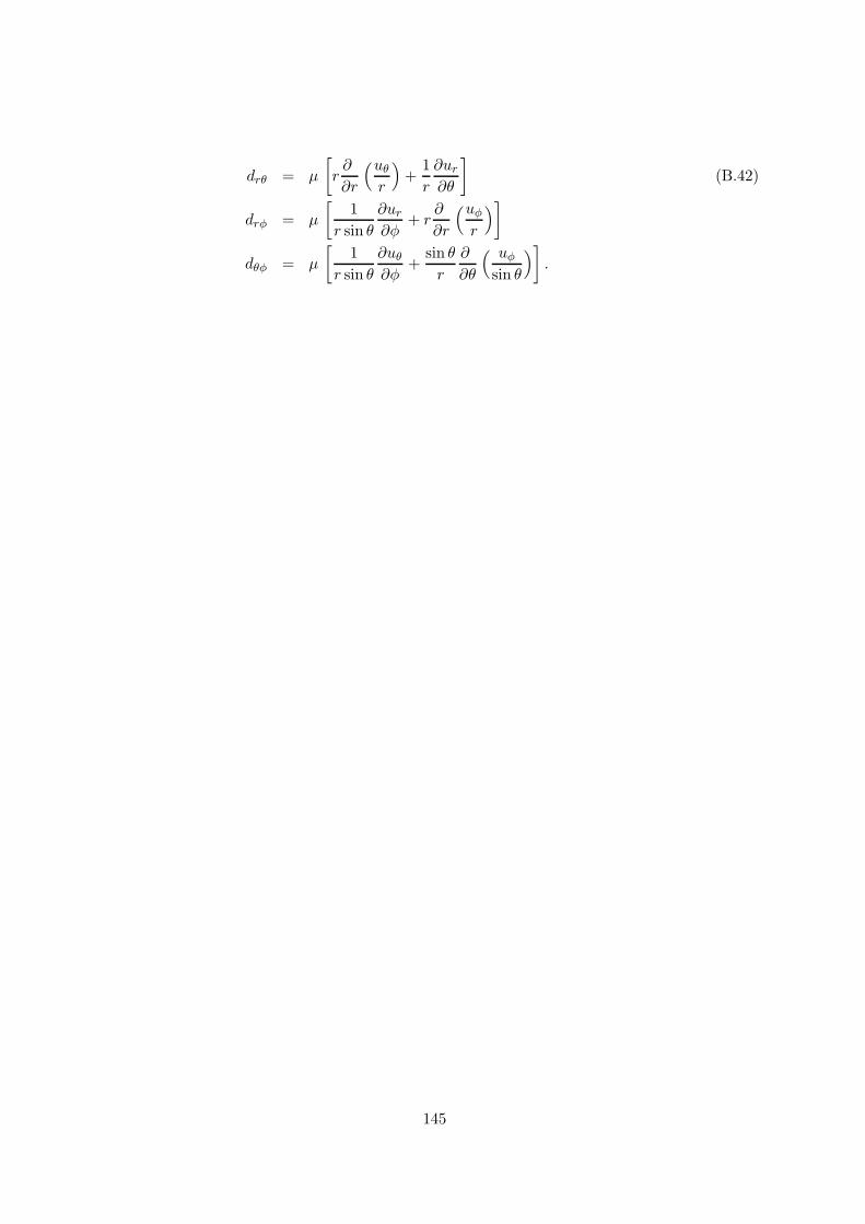
drθ = µ

[r∂

∂r

(uθ

r

)+

1r

∂ur

∂θ

](B.42)

drφ = µ

[1

r sin θ∂ur

∂φ+ r

∂

∂r

(uφ

r

)]

dθφ = µ

[1

r sin θ∂uθ

∂φ+

sin θr

∂

∂θ

( uφ

sin θ

)].

145

Appendix C

Flow field for a given volumeexpansion and vorticity

C.1 Flow field for a given volume expansion

There exists an exact solution of the Poisson equation (2.28). For a three-dimensional spaceit is given by

Φe(x) = − 14π

∫ ∫ ∫V

∆(x′)s

dV ′ (C.1)

where s = (x−x′)2+(y−y′)2+(z−z′)21/2 is the distance between x en x′ and dV ′ = dx′dy′dz′.The velocity field then follows by taking the gradient of (C.1). (Note that we should take thegradient only with respect to the coordinate x and not with respect to x′ because the latter isonly an integration variable.) The result reads

ue ≡ ∇Φe =14π

∫ ∫ ∫V

ss3

∆(x′)dV ′ (C.2)

where s is the connecting vector between x′ and x, i.e. s = (x− x′, y − y′, z − z′). The function

G(x,x′) = − 1

4πs= − 1

4π√

(x− x′)2 + (y − y′)2 + (z − z′)2(C.3)

which appears in (C.1) is sometime denoted as the Green’s function of the Poisson equation.In section 2.4.1 we have seen that the Green’s function can be interpreted in physical termsas a source/sink flow with unit strength. From this interpretation it follows that the Green’sfunction satisfies the equation

∇2x′ G

(x,x′) = δ

(x− x′) (C.4)

where the index on the nabla operator means that it should be applied only to the variable x′.The δ (x − x′) is the Dirac delta function, which is a function that is everywhere zero exceptat x′ = x where it is infinite such that the integral over all space is equal to 1. This meansthat the delta function is singular at x = x′. An important property of the delta function isgiven by the expression ∫ ∫ ∫

Vδ(x − x′) f

(x′) dV ′ = f (x)

146

With the definition (C.4) of the Green’s function we can write the solution of the Poissonequation (2.28) as

Φe(x) =∫ ∫ ∫

VG(x,x′)∆(x′)dV ′ (C.5)

This expression shows that the solution of the Poisson equation can be written as a weightedsum of all contributions over the whole flow region. In other words at each position in spacex the solution is influenced by the contributions ∆(x′) at every position. This property of thesolution is generally denoted as elliptic and it is a general property of the incompressible flowfield.

For two dimensions the solution of (2.28) is given by

Φex) =12π

∫ ∫V

ln(σ)∆(x′)dV ′ (C.6)

with σ = (x− x′)2 + (y − y′)21/2 and dV ′ = dx′dy′. For the velocity field then follows

ue ≡ ∇Φe =12π

∫ ∫V

σ

σ2∆(x′)dV ′. (C.7)

where σ denotes the vector σ = (x, y).In this two-dimensional case the Green’s function for the Poisson equation reads

G(x,x′) =

12π

ln(σ) =12π

ln(√

(x− x′)2 + (y − y′)2). (C.8)

As also shown in section 2.4.1 this solution can be interpreted as a source/sink with unitstrength in two dimensions. The general solution of the Poisson equation in two dimensioncan then be written in an analogous as (C.5) but now with an integration running over two-dimensional space.

C.2 Flow field for a given vorticity, ω.

In section 2.4.2 we have argued that (2.26) can be solved by introducing a vector potential Bv

which satisfies ue = ∇×Bv. However, the problem immediately presents itself that the Bv cannot be uniquely determined. For instance consider B′

v = Bv + grad Φ where Φ is any (twicedifferentiable) scalar function. The it from the condition ∇× gradΦ ≡ 0 that both B′

v and Bv

lead to the same velocity field. Let us now fix this non-uniqueness by demanding that Bv alsosatisfies divBv = 0 which can be always accomplished by choosing an appropriate function Φ.

Substitution of the vector potential Bv in ∇×uv = ω then results in the following equation

∇×∇× Bv = ∇ (∇ · Bv) − (∇ · ∇)Bv = ω.

or with the condition for Bv mentioned above we find

∇2Bv = −ω. (C.9)

This is again a a Poisson equation for which we have found the Green’s function in appendixC.1. Following the expression (C.5)the solution of (C.9) becomes

Bv(x) =∫ ∫ ∫

VG(x,x)ω(x′) dV ′ (C.10)

147

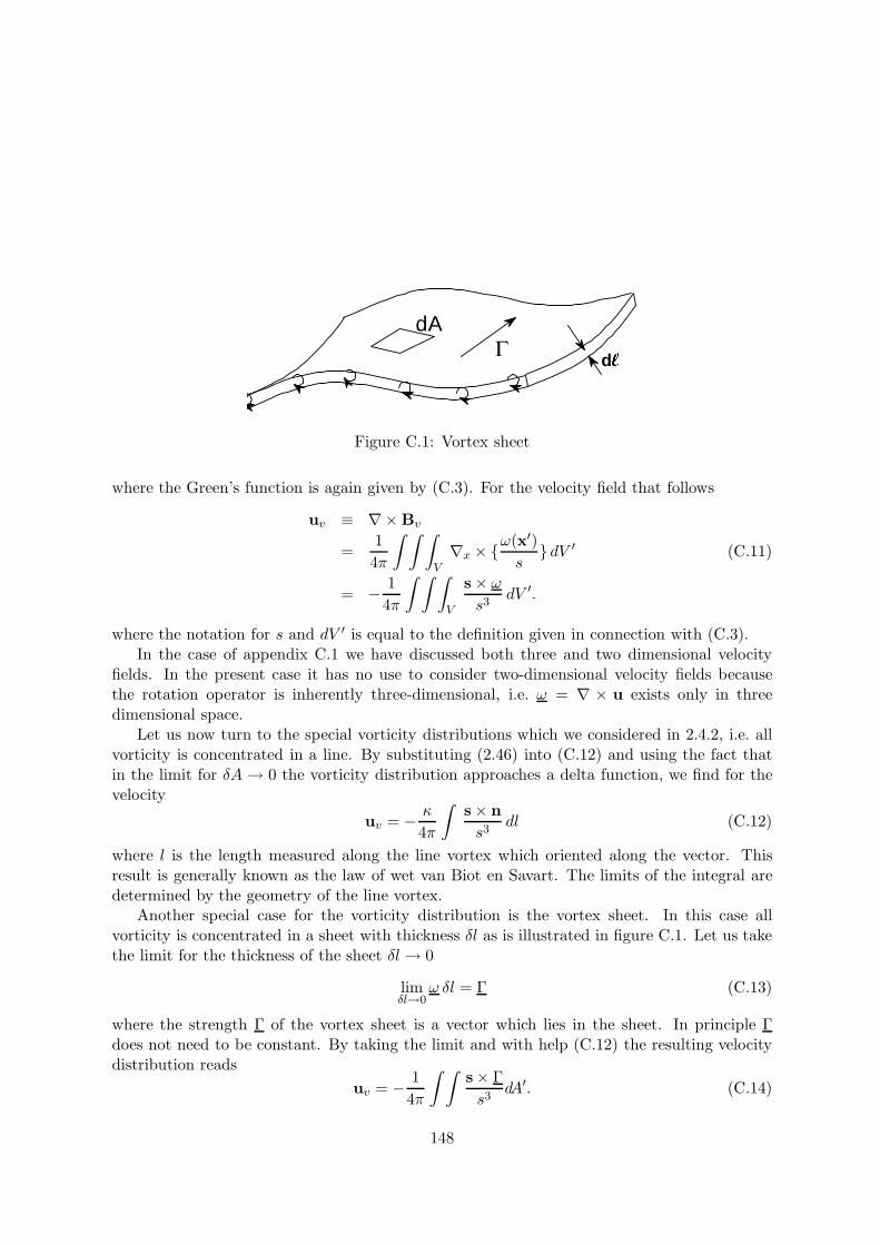
dAΓ d

Figure C.1: Vortex sheet

where the Green’s function is again given by (C.3). For the velocity field that follows

uv ≡ ∇× Bv

=14π

∫ ∫ ∫V

∇x × ω(x′)s

dV ′ (C.11)

= − 14π

∫ ∫ ∫V

s × ω

s3dV ′.

where the notation for s and dV ′ is equal to the definition given in connection with (C.3).In the case of appendix C.1 we have discussed both three and two dimensional velocity

fields. In the present case it has no use to consider two-dimensional velocity fields becausethe rotation operator is inherently three-dimensional, i.e. ω = ∇ × u exists only in threedimensional space.

Let us now turn to the special vorticity distributions which we considered in 2.4.2, i.e. allvorticity is concentrated in a line. By substituting (2.46) into (C.12) and using the fact thatin the limit for δA → 0 the vorticity distribution approaches a delta function, we find for thevelocity

uv = − κ

4π

∫s× ns3

dl (C.12)

where l is the length measured along the line vortex which oriented along the vector. Thisresult is generally known as the law of wet van Biot en Savart. The limits of the integral aredetermined by the geometry of the line vortex.

Another special case for the vorticity distribution is the vortex sheet. In this case allvorticity is concentrated in a sheet with thickness δl as is illustrated in figure C.1. Let us takethe limit for the thickness of the sheet δl → 0

limδl→0

ω δl = Γ (C.13)

where the strength Γ of the vortex sheet is a vector which lies in the sheet. In principle Γdoes not need to be constant. By taking the limit and with help (C.12) the resulting velocitydistribution reads

uv = − 14π

∫ ∫s× Γs3

dA′. (C.14)

148

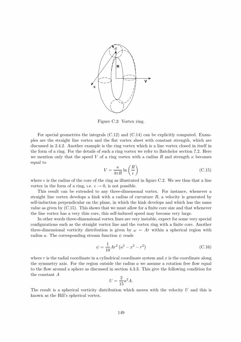
R

Vκ

ε

Figure C.2: Vortex ring.

For special geometries the integrals (C.12) and (C.14) can be explicitly computed. Exam-ples are the straight line vortex and the flat vortex sheet with constant strength, which arediscussed in 2.4.2. Another example is the ring vortex which is a line vortex closed in itself inthe form of a ring. For the details of such a ring vortex we refer to Batchelor section 7.2. Herewe mention only that the speed V of a ring vortex with a radius R and strength κ becomesequal to

V =κ

4πRln(R

ε

)(C.15)

where ε is the radius of the core of the ring as illustrated in figure C.2. We see thus that a linevortex in the form of a ring, ı.e. ε→ 0, is not possible.

This result can be extended to any three-dimensonal vortex. For instance, whenever astraight line vortex develops a kink with a radius of curvature R, a velocity is generated byself-induction perpendicular on the plane, in which the kink develops and which has the samevalue as given by (C.15). This shows that we must allow for a finite core size and that wheneverthe line vortex has a very thin core, this self-induced speed may become very large.

In other words three-dimensional vortex lines are very instable, expect for some very specialconfigurations such as the straight vortex line and the vortex ring with a finite core. Anotherthree-dimensional vorticity distribution is given by ω = Ar within a spherical region withradius a. The corresponding stream function ψ reads

ψ =110Ar2

(a2 − x2 − r2

)(C.16)

where r is the radial coordinate in a cylindrical coordinate system and x is the coordinate alongthe symmetry axis. For the region outside the radius a we assume a rotation free flow equalto the flow around a sphere as discussed in section 4.3.3. This give the following condition forthe constant A

U =215a2A.

The result is a spherical vorticity distribution which moves with the velocity U and this isknown as the Hill’s spherical vortex.

149

Appendix D

General properties of potential flows

In this appendix we shall prove the general properties of potential flows that have been intro-duced in section 4.2. Point of departure is a singly-connected region V shown in figure 4.1, inwhich a potential flow is given with potential Φ and with boundary conditions for the velocitycomponent in the direction of the normals on the surface A1 and A2 that border the volumeV .

D.1 The solution for the potential Φ is single valued

To prove this property we take two points P and O in V . The value of Φ in O is given by ΦO.The value of Φ in P follows then from

ΦP = ΦO +∫ P

O

∂Φ∂s

ds

ΦP = ΦO +∫ P

O∇Φ · ds

ΦP = ΦO +∫ P

Ov · ds (D.1)

where the path of integration between O and P lies in V but for the rest is arbitrary. The Φ isnow single valued when ΦP is independent of the path of integration. To this end we computethe integral (D.1) along two different integration paths where we integrate along path 1 fromO to P and along path 2 from P to O. In other words we compute the integral along a closedreducible curve, which we call Γ. The condition of single valuedness implies that the integralalong path 1 from O to P must be equal but opposite to the integral along path 2 from P toO. The difference in sign follows from the difference in the direction of integration. In otherwords the circle integral along Γ must be equal to zero, i.e.∮

Γv · ds = 0. (D.2)

To prove this last result we take a surface of which the edge is given by Γ. Because V is singlyconnected it is always possible to find such a surface, which at the same time is totally insideV . On this surface we apply the theorem of Stokes (A.11). Because ω = ∇×u = ∇×∇Φ ≡ 0in V (D.2) follows, so that the single valuedness of is Φ proven.

150

D.2 The integral of the kinetic energy

Let us consider ∫ ∫ ∫V

u · u dV =∫ ∫

A2

Φu · n2 dA−∫ ∫

A1

Φu · n1 dA. (D.3)

To prove this relation we consider the vector relationship (A.17). Because divu = 0 it followsthat ∇ · (Φu) = u · ∇Φ = u · u. Next we compute∫ ∫ ∫

u · u dV =∫ ∫ ∫

∇ · (Φu) dV. (D.4)

Application of the divergence or Gauss theorem (A.9) to (D.4) leads then directly to (D.3),where one has to take into account that the n1 is an inner normal.

D.3 Uniqueness

With help of (D.3) we can prove that for given boundary conditions on A1 and A2 the solutionof the potential Φ is unique apart from an additive constant. In other words the solution ofthe Laplace equation and with that the velocity is completely determined by the boundaryconditions. The proof goes as follows. Suppose that there are two different solutions Φ andΦ∗ in V with ∇Φ = u en ∇Φ∗ = u∗, which both satisfy the same boundary conditions. Thismeans that on A1 and A2 we have ∂Φ/∂n = ∂Φ∗/∂n or u · n = u∗ · n. The solution is uniqueif we can show that Φ ≡ Φ∗. To prove this we apply (D.3) to Φ − Φ∗ with as result∫ ∫ ∫

V(u − u∗)2 dV =

∫ ∫A2

(Φ − Φ∗)(u − u∗) · n2 dA−∫ ∫A1

(Φ − Φ∗)(u − u∗) · n1 dA. (D.5)

Because u ≡ u∗ on A1 as well as on A2 it follows that the right-hand side of (D.5) is equal tozero. With this it follows that u = u∗ everywhere in V and this implies that Φ = Φ∗ apartfrom an additive constant. This constant has further no consequences for the velocity field.

The property of uniqueness has as a consequence that when the boundary conditions on A1

and A2 change, the velocity field changes instantaneously everywhere in the volume V . In otherwords the transfer of information of the boundary to everywhere in the velocity field is infinitelyfast. The physical background of this result lies in the assumption of incompressibility (2.6), asa result of which the speed of sound, which is the propagation velocity of small disturbances,becomes infinitely large.

D.4 Minimal energy

It turns out that the kinetic energy of a potential flow is minimal. To prove this result weconsider two solutions for the velocity field u and u∗ of our flow problem in V , with u a potentialflow and thus rotation free, while the velocity field u∗ has rotation. Both solutions satisfy the

151

equations of motion and are thus divergence free. They also satisfy the same conditions on theboundary of the flow domain. It follows now that

T ∗ − T =12ρ

∫ ∫ ∫V

(u∗ 2 − u2) dV

=12ρ

∫ ∫ ∫V

(u∗ − u)2 dV + ρ

∫ ∫ ∫V

(u∗ − u) · u dV. (D.6)

Consider now the identity ∇·(u∗−u)Φ = ∇ · (u∗−u)Φ+(u∗−u) ·∇Φ, where as a resultof the property of incompressible or divergence free flow, the first terms on the right-hand sideare equal to zero, so that ∇ · (u∗ − u)Φ = (u∗ − u) · u. It then follows after substitution in(D.6) that

T ∗ − T =12ρ

∫ ∫ ∫V

(u∗ − u)2 dV + ρ

∫ ∫ ∫V

∇ · (u∗ − u)Φ dV

=12ρ

∫ ∫ ∫V

(u∗ − u)2 dV + ρ

∫ ∫A

Φ(u∗ − u) · n dA

=12ρ

∫ ∫ ∫V

(u∗ − u)2 dV > 0 (D.7)

where we have made use of the divergence theorem (A.9) and the fact that u∗ and u satisfythe same boundary conditions on A. From (D.7) it then follows that for every u∗ the potentialflow u has less energy.

D.5 Maximum value of the potential

Based on a general property of the Laplace equation it follows that potential Φ can adoptno extreme values inside a volume V where an extreme value means either a minimum or amaximum. In other words a maximum of a minimum of a potential can thus only occur on theboundaries A of the domain where the potential flow is valid. To prove this result we write theLaplace equation as ∇ · ∇Φ = 0 and apply to the result the divergence theorem (A.9). Theresult reads ∫ ∫

A∇Φ · n dA = 0. (D.8)

Now we assume that somewhere in V the Φ adopts an extreme value. Let us construct aroundthis point a small sphere with surface A and apply (D.8). If the sphere is chosen close enougharound the point in question, the value of ∇Φ·n around the surface of the sphere will everywherehave the same sign, i.e. negative for a maximum and positive for a minimum. However, it isalso clear that (D.8) can not be satisfied when ∇Φ · n have the same sign everywhere on thissurface A. In other words it is not possible to have a maximum of minimum value of Φ insidethe flow domain V .

152

Appendix E

The theory of complex functions fortwo-dimensional potential flows

Let us consider a two-dimensional potential flow with potential Φ and with velocity componentsu and v as a function of the coordinates x and y. At the same time we introduce a streamfunction ψ. By definition the following expressions are then valid

u =∂Φ∂x

, v =∂Φ∂y

(E.1)

u =∂ψ

∂y, v = −∂ψ

∂x. (E.2)

These relationships can be rewritten as

∂Φ∂x

=∂ψ

∂y

∂Φ∂y

= −∂ψ∂x

. (E.3)

From (E.3) It follow directly that the lines where Φ = constant (equi-potential lines) areperpendicular to the lines where ψ = constant (streamlines), because

grad Φ · gradψ = 0 (E.4)

or the functions Φ en ψ form a system of orthogonal linesHowever, the relations (E.3) have an important meaning in the theory of complex functions.

There they are called the Cauchy-Riemann relations. Therefore, we can make use of complexfunction theory for the computation of tho-dimensional potential flows. Before we considerthis, we shall first repeat some basic facts of complex function theory.

E.1 Analytical function

Let us define the complex variable z according to

z = x+ i y (E.5)

153

where i is by definition equal to√−1. The x is called by definition the real part (z) and the

y the imaginary part (z) of z. The z can be presented as a coordinate in a two-dimensionalor z-plane, where we place the real part along the x-axis and the imaginary part along they-axis.

Let us introduce the following complex function

w(z) = Φ + i ψ (E.6)

where the potential Φ(x, y) forms the real and the steam function ψ(x, y) the imaginary part.If Φ(x, y) and ψ(x, y) satisfy the Cauchy-Riemann relations (E.3) we call w(z) an analytic

function. The term analytic implies that in each point z the derivative dw/dz is unique anddoes not depend on the direction in the z-plane, in which the derivative is taken.

For a formal proof we refer to a textbook on complex function theory. Here we shallillustrate the notion, analytic function, by computing the derivative of w(z) in two directions.First we take a direction along the x-axis. In that case dz = dx and as a result it follows from(E.5) that

dw

dz=

∂Φ∂x

+ i∂ψ

∂x= u − i v. (E.7)

Second we take the y-axis as the direction of differentiation and this leads with (E.5) todz = i dy, so that

dw

dz=

1i

∂Φ∂y

+∂ψ

∂y

= u − i v (E.8)

where we have made use of the Cauchy-Riemann equations (E.3).Both differentiation direction thus lead ot the same result.

E.2 Complex potential

Let us retrun to the two-dimensional potential flows. In that case we call the function w(z)defined according to (E.6) the complex potential. The Cauchy-Riemann equations (E.3) forthe potential and stream function guarantee that w(z) is an analytic function. At the sametime we have found that according to relations (E.7) and (E.8) the derivative of of w can berelated to the velocity components u and v.

The result that have found above, can be also turned around. This means that any analyticfunction can be interpreted as a two-dimensional potential flow. Some examples are:

• parallel flow:w = Uz (E.9)

where U , which in principle may be complex, gives the direction and magnitude of theparallel flow.

• source/sink in z0:w =

m

2πln(z − z0) (E.10)

where m represent the strength of the source/sink.

154

• dipole in z0:w = − µ

2π(z − z0)(E.11)

where µ is a complex constant, which determines the direction and strength of the dipole.

• point vortex in z0:

w = − i κ2π

ln(z − z0) (E.12)

where κ gives the strength or circulation of the point vortex.

It is left as an exercise to compare these complex potentials with the expressions for asource/sink and dipole flow that we have found in section 2.4.1. Here we shall go in some detailson the potential of the point vortex, which as mentioned in section 2.4.2 can be connected tothe straight line vortex. To show the connection to the results that we have derived in thatsection we split (E.12) with z0 = 0 in its real and imaginary part according to

Φ =κ

2πθ (E.13)

ψ = − κ

2πln r (E.14)

where we have used the representation of the complex variable z in the form

z = r eiθ (E.15)

where r is called the magnitude and θ the argument of z. The relation with the real andimaginary part is given by

x = r cos θy = r sin θ. (E.16)

From (E.14) it follows that the stream lines are circles, which have the position of the pointvortex as centre. At the same time it follows that the velocity is given by

ur = 0

uθ =κ

2πr, (E.17)

which is consistent with (2.48).With help of (E.9) and (E.11) we can formulate now the following complex potential

w = −Uz − µ

2πz(E.18)

where the µ is taken as a real number. This means that the dipole vector is chosen alongthe x- axis. The result is the complex potential of the flow around a cylinder with radiusa =

√µ/(2πU), which have discussed in some detail in section 4.4.1

155

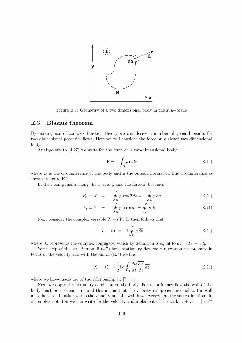
Bx

y

zn

ds

Figure E.1: Geometry of a two dimensional body in the x, y−plane

E.3 Blasius theorem

By making use of complex function theory we can derive a number of general results fortwo-dimensional potential flows. Here we will consider the force on a closed two-dimensionalbody.

Analogously to (4.27) we write for the force on a two-dimensional body

F = −∮

Bpn ds (E.19)

where B is the circumference of the body and n the outside normal on this circumference asshown in figure E.1.

In their components along the x- and y-axis the force F becomes

Fx ≡ X = −∮

Bp cos θ ds = −

∮Bp dy (E.20)

Fy ≡ Y = −∮

Bp sin θ ds =

∮Bp dx. (E.21)

Next consider the complex variable X − i Y . It then follows that

X − i Y = −i∮

Bp dz (E.22)

where dz represents the complex conjugate, which by definition is equal to dz = dx − i dy.With help of the law Bernouilli (4.7) for a stationary flow we can express the pressure in

terms of the velocity and with the aid of (E.7) we find

X − i Y =12i ρ

∮B

dw

dz

dw

dzdz (E.23)

where we have made use of the relationship | z |2= zz.Next we apply the boundary condition on the body. For a stationary flow the wall of the

body must be a stream line and this means that the velocity component normal to the wallmust be zero. In other words the velocity and the wall have everywhere the same direction. Ina complex notaiton we can write for the velocity and a element of the wall: u + i v = |u |ei θ

156

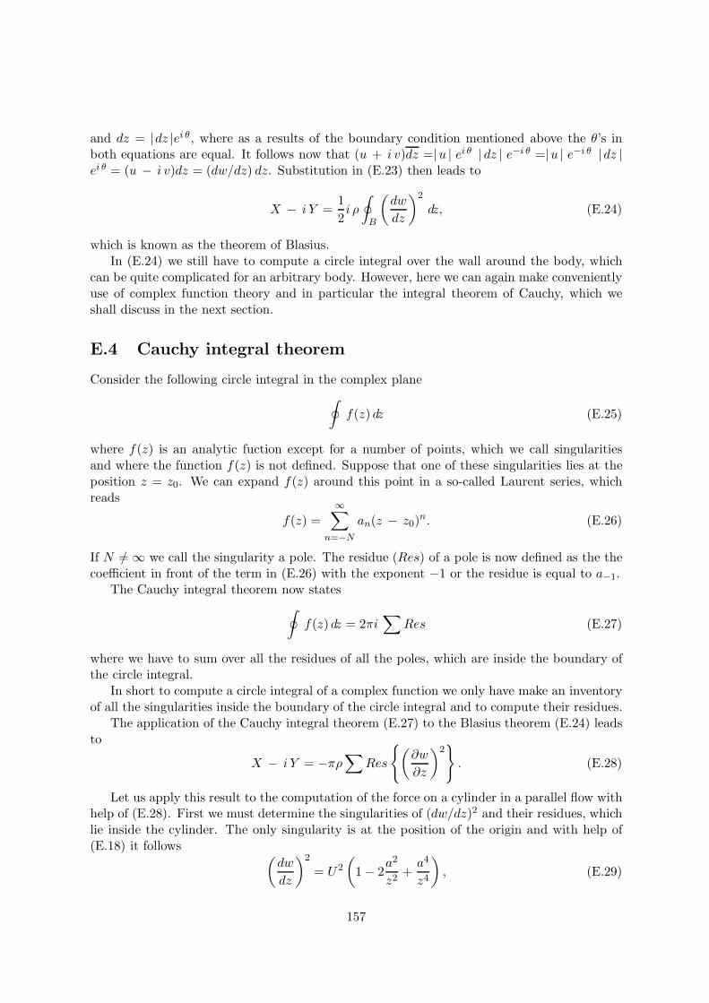
and dz = |dz |ei θ, where as a results of the boundary condition mentioned above the θ’s inboth equations are equal. It follows now that (u + i v)dz =|u | ei θ |dz | e−i θ =|u | e−i θ |dz |ei θ = (u − i v)dz = (dw/dz) dz. Substitution in (E.23) then leads to

X − i Y =12i ρ

∮B

(dw

dz

)2

dz, (E.24)

which is known as the theorem of Blasius.In (E.24) we still have to compute a circle integral over the wall around the body, which

can be quite complicated for an arbitrary body. However, here we can again make convenientlyuse of complex function theory and in particular the integral theorem of Cauchy, which weshall discuss in the next section.

E.4 Cauchy integral theorem

Consider the following circle integral in the complex plane∮f(z) dz (E.25)

where f(z) is an analytic fuction except for a number of points, which we call singularitiesand where the function f(z) is not defined. Suppose that one of these singularities lies at theposition z = z0. We can expand f(z) around this point in a so-called Laurent series, whichreads

f(z) =∞∑

n=−N

an(z − z0)n. (E.26)

If N =/ ∞ we call the singularity a pole. The residue (Res) of a pole is now defined as the thecoefficient in front of the term in (E.26) with the exponent −1 or the residue is equal to a−1.

The Cauchy integral theorem now states∮f(z) dz = 2πi

∑Res (E.27)

where we have to sum over all the residues of all the poles, which are inside the boundary ofthe circle integral.

In short to compute a circle integral of a complex function we only have make an inventoryof all the singularities inside the boundary of the circle integral and to compute their residues.

The application of the Cauchy integral theorem (E.27) to the Blasius theorem (E.24) leadsto

X − i Y = −πρ∑

Res

(∂w

∂z

)2. (E.28)

Let us apply this result to the computation of the force on a cylinder in a parallel flow withhelp of (E.28). First we must determine the singularities of (dw/dz)2 and their residues, whichlie inside the cylinder. The only singularity is at the position of the origin and with help of(E.18) it follows (

dw

dz

)2

= U2

(1 − 2

a2

z2+a4

z4

), (E.29)

157

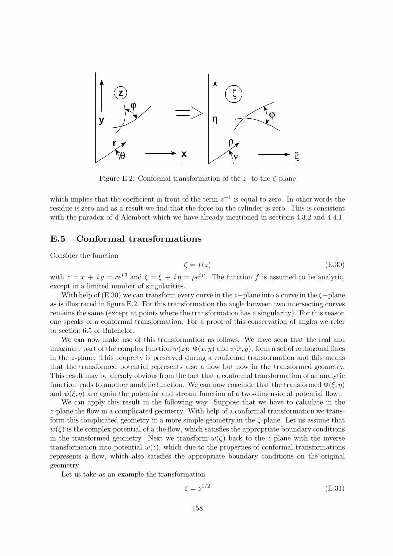
x

y

z

ξ

ζ

ϕϕ

η

νρr

θ

Figure E.2: Conformal transformation of the z- to the ζ-plane

which implies that the coefficient in front of the term z−1 is equal to zero. In other words theresidue is zero and as a result we find that the force on the cylinder is zero. This is consistentwith the paradox of d’Alembert which we have already mentioned in sections 4.3.2 and 4.4.1.

E.5 Conformal transformations

Consider the functionζ = f(z) (E.30)

with z = x + i y = rei θ and ζ = ξ + i η = ρei ν . The function f is assumed to be analytic,except in a limited number of singularities.

With help of (E.30) we can transform every curve in the z−plane into a curve in the ζ−planeas is illustrated in figure E.2. For this transformation the angle between two intersecting curvesremains the same (except at points where the transformation has a singularity). For this reasonone speaks of a conformal transformation. For a proof of this conservation of angles we referto section 6.5 of Batchelor.

We can now make use of this transformation as follows. We have seen that the real andimaginary part of the complex function w(z): Φ(x, y) and ψ(x, y), form a set of orthogonal linesin the z-plane. This property is preserved during a conformal transformation and this meansthat the transformed potential represents also a flow but now in the transformed geometry.This result may be already obvious from the fact that a conformal transformation of an analyticfunction leads to another analytic function. We can now conclude that the transformed Φ(ξ, η)and ψ(ξ, η) are again the potential and stream function of a two-dimensional potential flow.

We can apply this result in the following way. Suppose that we have to calculate in thez-plane the flow in a complicated geometry. With help of a conformal transformation we trans-form this complicated geometry in a more simple geometry in the ζ-plane. Let us assume thatw(ζ) is the complex potential of a the flow, which satisfies the appropriate boundary conditionsin the transformed geometry. Next we transform w(ζ) back to the z-plane with the inversetransformation into potential w(z), which due to the properties of conformal transformationsrepresents a flow, which also satisfies the appropriate boundary conditions on the originalgeometry.

Let us take as an example the transformation

ζ = z1/2 (E.31)

158

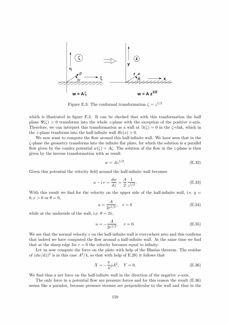
x

yz

ξ

ζ

η

ζw = A w = A z1/2

rθ

ρν

Figure E.3: The conformal transformation ζ = z1/2

which is illustrated in figure E.3. It can be checked that with this tranformation the halfplane (ζ) > 0 transforms into the whole z-plane with the exception of the positive x-axis.Therefore, we can interpret this transformation as a wall at (ζ) = 0 in the ζ-vlak, which inthe z-plane tranforms into the half-infinite wall Re(x) > 0.

We now want to compute the flow around this half-infinite wall. We have seen that in theζ-plane the geometry transforms into the infinite flat plate, for which the solution is a parallelflow given by the comlex potential w(ζ) = Aζ. The solution of the flow in the z-plane is thengiven by the inverse transformation with as result

w = Az1/2. (E.32)

Given this potential the velocity field around the half-infinite wall becomes

u− i v =dw

dz=A

21z1/2

. (E.33)

With this result we find for the velocity on the upper side of the half-infinite wall, i.e. y =0, x > 0 or θ = 0,

u =A

2r1/2, v = 0 (E.34)

while at the underside of the wall, i.e. θ = 2π,

u = − A

2r1/2, v = 0. (E.35)

We see that the normal velocity v on the half-infinite wall is everywhere zero and this confirmsthat indeed we have computed the flow around a half-infinite wall. At the same time we findthat at the sharp edge for r = 0 the velocity becomes equal to infinity.

Let us now compute the force on the plate with help of the Blasius theorem. The residueof (dw/dz)2 is in this case A2/4, so that with help of E.28) it follows that

X = −π4ρA2, Y = 0. (E.36)

We find thus a net force on the half-infinite wall in the direction of the negative x-axis.The only force in a potential flow are pressure forces and for this reason the result (E.36)

seems like a paradox, because pressure stresses are perpendicular to the wall and thus in the

159

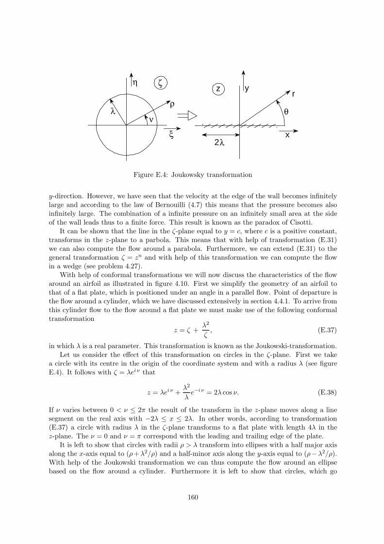
zr

2x

yζη

ξ

ν

ρ

λ

λ θ

Figure E.4: Joukowsky transformation

y-direction. However, we have seen that the velocity at the edge of the wall becomes infinitelylarge and according to the law of Bernouilli (4.7) this means that the pressure becomes alsoinfinitely large. The combination of a infinite pressure on an infinitely small area at the sideof the wall leads thus to a finite force. This result is known as the paradox of Cisotti.

It can be shown that the line in the ζ-plane equal to y = c, where c is a positive constant,transforms in the z-plane to a parbola. This means that with help of transformation (E.31)we can also compute the flow around a parabola. Furthermore, we can extend (E.31) to thegeneral transformation ζ = zn and with help of this transformation we can compute the flowin a wedge (see problem 4.27).

With help of conformal transformations we will now discuss the characteristics of the flowaround an airfoil as illustrated in figure 4.10. First we simplify the geometry of an airfoil tothat of a flat plate, which is positioned under an angle in a parallel flow. Point of departure isthe flow around a cylinder, which we have discussed extensively in section 4.4.1. To arrive fromthis cylinder flow to the flow around a flat plate we must make use of the following conformaltransformation

z = ζ +λ2

ζ, (E.37)

in which λ is a real parameter. This transformation is known as the Joukowski-transformation.Let us consider the effect of this transformation on circles in the ζ-plane. First we take

a circle with its centre in the origin of the coordinate system and with a radius λ (see figureE.4). It follows with ζ = λei ν that

z = λei ν +λ2

λe−i ν = 2λ cos ν. (E.38)

If ν varies between 0 < ν ≤ 2π the result of the transform in the z-plane moves along a linesegment on the real axis with −2λ ≤ x ≤ 2λ. In other words, according to transformation(E.37) a circle with radius λ in the ζ-plane transforms to a flat plate with length 4λ in thez-plane. The ν = 0 and ν = π correspond with the leading and trailing edge of the plate.

It is left to show that circles with radii ρ > λ transform into ellipses with a half major axisalong the x-axis equal to (ρ+λ2/ρ) and a half-minor axis along the y-axis equal to (ρ−λ2/ρ).With help of the Joukowski transformation we can thus compute the flow around an ellipsebased on the flow around a cylinder. Furthermore it is left to show that circles, which go

160

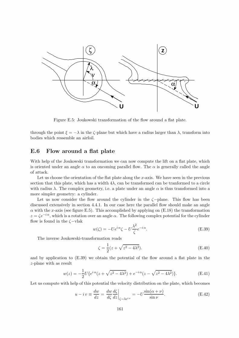
U U

zζ

λνα α

Figure E.5: Joukowski transformation of the flow around a flat plate.

through the point ξ = −λ in the ζ-plane but which have a radius larger than λ, transform intobodies which ressemble an airfoil.

E.6 Flow around a flat plate

With help of the Joukowski transformation we can now compute the lift on a flat plate, whichis oriented under an angle α to an oncoming parallel flow. The α is generally called the angleof attack.

Let us choose the orientation of the flat plate along the x-axis. We have seen in the previoussection that this plate, which has a width 4λ, can be transformed can be tranformed to a circlewith radius λ. The complex geometry, i.e. a plate under an angle α is thus transformed into amore simpler geometry: a cylinder.

Let us now consider the flow around the cylinder in the ζ−plane. This flow has beendiscussed extensively in section 4.4.1. In our case here the parallel flow should make an angleα with the x-axis (see figure E.5). This accomplished by applying on (E.18) the transformationz = ζe−i α, which is a rotation over an angle α. The following complex potential for the cylinderflow is found in the ζ−vlak

w(ζ) = −Uei αζ − Uλ2

ζe−i α. (E.39)

The inverse Joukowski-transformation reads

ζ =12(z +

√z2 − 4λ2). (E.40)

and by application to (E.39) we obtain the potential of the flow around a flat plate in thez-plane with as result

w(z) = −12Uei α(z +

√z2 − 4λ2) + e−i α(z −

√z2 − 4λ2). (E.41)

Let us compute with help of this potential the velocity distribution on the plate, which becomes

u− i v ≡ dw

dz=dw

dζ

dζ

dz

∣∣∣∣ζ=λei ν

= −U sin(α+ ν)sin ν

. (E.42)

161

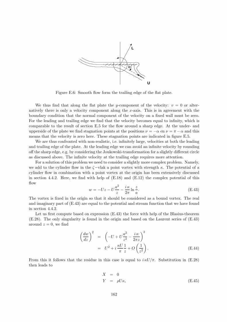
U

α

L

Figure E.6: Smooth flow form the trailing edge of the flat plate.

We thus find that along the flat plate the y-component of the velocity: v = 0 or alter-natively there is only a velocity component along the x-axis. This is in agreement with theboundary condition that the normal component of the velocity on a fixed wall must be zero.For the leading and trailing edge we find that the velocity becomes equal to infinity, which iscomparable to the result of section E.5 for the flow around a sharp edge. At the under- andupperside of the plate we find stagnation points at the positions ν = −α en ν = π−α and thismeans that the velocity is zero here. These stagnation points are indicated in figure E.5.

We are thus confronted with non-realistic, i.e. infinitely large, velocities at both the leadingand trailing edge of the plate. At the leading edge we can avoid an infinite velocity by roundingoff the sharp edge, e.g. by considering the Joukowski-transformation for a slightly different circleas discussed above. The infinite velocity at the trailing edge requires more attention.

For a solution of this problem we need to consider a slightly more complex problem. Namely,we add to the cylinder flow in the ζ−vlak a point vortex with strength κ. The potential of acylinder flow in combination with a point vortex at the origin has been extensively discussedin section 4.4.2. Here, we find with help of (E.18) and (E.12) the complex potential of thisflow

w = −Uz − Ua2

z− i κ

2πlnz

a. (E.43)

The vortex is fixed in the origin so that it should be considered as a bound vortex. The realand imaginary part of (E.43) are equal to the potential and stream function that we have foundin section 4.4.2.

Let us first compute based on expression (E.43) the force with help of the Blasius-theorem(E.28). The only singularity is found in the origin and based on the Laurent series of (E.43)around z = 0, we find

(dw

dz

)2

=(−U + U

a2

z2− i κ

2πz

)2

= U2 + iκU

π

1z

+O

(1z2

). (E.44)

From this it follows that the residue in this case is equal to i κU/π. Substitution in (E.28)then leads to

X = 0Y = ρUκ, (E.45)

162

which shows in the x-direction a zero drag force. In the y-direction we find a lift force equalto L = ρUκ, which consistent with the result found in section 4.4.2.

The addition of the line vortex means that to the potential (E.39) an term (−i κ)/(2π) ln(ζ/λ)is added. Let us compute for this potential again the velocity distribution on the plate. Theresult reads

u− i v ≡ dw

dz= −U sin(α + ν) + κ

4πUλ

sin ν. (E.46)

The circulation κ is in principle still arbitrary. We now choose this circulation such that astagnation point falls on the trailing edge. In that case we have no longer an infinite velocityon the traling edge as is illustrated in figure E.6. The trailing edge corresponds with ν = πand application of this condition for the circulation then leads to

sin(α+ π) +κ

4πUλ= 0, (E.47)

which provides an equation for κ. This equation is known as the Kutta-Joukowski condition.This condition states that around the flat plate a circulation is generated, which causes asmooth flow from the trailing edge and thus infinite velocities are avoided. The same conditioncan be generalised for the flow around an airfoil with a sharp trailing edge.

In a conformal transformation the singularities and their residues remain invariant. As wehave seen that there is a lift force on the cylinder with circulation, this means that there isalso a lift force on the flat plate due to the circulation and this force is again

L = ρκU

= 4πρU2λ sinα (E.48)

where we have used (E.47) to eliminate the κ. This lift force can be expresses in terms of alift coefficient cL, given by (4.57), as we have shown in section 4.4.2.

Note that the lift force is perpendicular on the parallel flow as illustrated in E.6. Thisis consistent with the fact that the drag is again zero in correspondence with the paradox ofd’Alembert. However, in a potential flow we have only pressure stresses, which are perpendic-ular to the surface, on which they act, and therefore one would perhaps expect that the liftforce should be perpendicular to the flat plate. However, remember that in the case of the flatplate we have still an infinite velocity at leading edge of the plate. To this configuration appliesthe paradox of Cisotti, which makes that the resultant force on the plate is perpendicular tothe parallel flow.

163

Appendix F

Crocco’s theorm

In section 5.3 we have consider the energy integral and we have proved that for the incom-pressible flow of an ideal fluid the quantity H defined in (5.23) is constant along a stream line.In this appendix we shall consider how H depends on the spatial coordinates.

To this end we consider the definition of S (5.12) but now expressed as a spatial gradient

T∇S = ∇E + p∇1ρ. (F.1)

Next we take gradient of (5.20)

∇H = ∇E + ∇(

12u2

i

)+ ∇

(p

ρ

)+ ∇Ψ. (F.2)

Because we consider in the first place the law of Bernouilli, we restrict ourselves to an idealfluid, for which the Euler equations are valid. For a stationary flow it follows from theseequations that

(u · ∇)u = −∇Ψ − 1ρ∇p. (F.3)

With the vector relationship (A.16) we can rewrite this equations as

∇(

12u2

)+ ∇Ψ +

1ρ∇p = u × ω (F.4)

where ω = ∇× u.By combination of (F.1), (F.2) and (F.4) the following expression results

∇H = T∇S + u× ω, (F.5)

which is known as Crocco’s theorem.

164

Appendix G

Stokes flow around a sphere

The solution of (6.54) must have in principle the following form: p, ω = f(x,U, a). As a resultof the boundary conditions (6.56) it follows that the solution must be linear in the velocity U.This conclusion allows us the make the following hypothesis for the pressure p = (U ·x)f(r/a)where r = |x|. Next it is known that p must be a standard solution of the Laplace equation.This is discussed further in section 2.9 of Batchelor. Based on this we find for the solution,which satisfies all conditions:

p− p0

µ= C

U · xr3

(G.1)

ω = CU × xr3

(G.2)

where C is a constant. By substitution of (G.1 ) and (G.2) into (6.54) and (6.55) it followsthat C in both equations has the same value.

Next we derive the from (G.2) the velocity field. Because the velocity is axi-symmetric, wecan make use of a Stokes stream function ψ, which is defined in (2.13). With the definition ofvorticity in spherical coordinates, as given in appendix B.3, it then follows

1r

∂ruθ

∂r− 1r

∂ur

∂θ= ωφ =

CUr sin θr3

, (G.3)

which leads tot he following equation for ψ

1r sin θ

∂2ψ

∂r2+

1r3∂

∂θ(

1sin θ

∂ψ

∂θ) = −CUr sin θ

r3. (G.4)

A particular solution of this equation can be found by substitution of ψ = U sin2 θf(r) withas result the following equation for f

d2f

dr2− 2fr2

= −Cr. (G.5)

The general solution of this ordinary differential equation, which is of the Euler type, reads

f = Ar2 +B

r+

12Cr (G.6)

165

where A and B are integration constants. Application of the boundary conditions (6.56) thenresult is

A = 0

C =32a (G.7)

B = −14a3.

166

Index

acceleration, 11–13, 16, 35, 36, 46, 67, 138centrifugal, 47, 96Coriolis, 47gravity, 35, 41, 54, 57, 80, 88pressure, 47sudden, 66

added mass, 66, 73advection, 11, 89, 125airfoil, 76, 124, 160

angle of attack, 76, 161chord, 76Kutta-Joukowski

con dition, 163sharp trailing edge, 76

amplitude, 77angle of attack, 76, 161angular velocity, 21, 22, 46, 54, 96, 104, 119Archimedes

law of, 41, 66axisymmetry, 17

Bassetterm of, 118

BatchelorBatchelor-Prandtl theorem, 52

bearingjournal, 104

Beltramiflow, 87

Bernouillilaw of, 57, 60, 63, 65, 72, 75, 78, 86,

100, 112, 127, 156, 160, 164Beta-plane, 55, 81Biot & Savart

law of, 29, 148Bjerknes

theorem of, 50Blasius

equation of, 128

profile, 129theorem of, 157, 159theorm of, 157

bluff body, 124, 130body

bluff, 124, 130force, 35, 88streamlined, 124

Bordacontraction, 61

boundary condition, 23, 44, 45, 55, 56, 64,67, 77

stress, 44velocity, 44

boundary layer, 95, 101, 122, 124, 125Blasius equation, 128Blasius profile, 129displacement thickness, 130equation, 127inner region, 126momentum integral, 131momentum thickness, 131outer layer, 127outer region, 125Prandtl, 128pressure, 127pressure gradient, 130separation, 130suction, 126thickness, 125, 126, 128, 129wall shear stress, 129

bubble, 45, 56, 67expanding, 68, 69potential flow, 68Stokes flow, 119

buoyancy, 41force, 67, 68, 117

Burgersvortex, 51

167

Cartesiancoordinate system, 135frame of reference, 12, 16geometry, 18, 90tensor, 11, 138

Cauchyfirst fundamental stress theorem, 37second fundamental stress theorem, 37vorticity equation, 51

Cauchy-Riemannrelations, 153

cavitation, 59, 69channel

convergent, 105circulation, 28, 47, 74Cisotti

paradox of, 160, 163closed system, 82coefficient

pressure, 116complex

analytic function, 154argument, 155Cauchy-Riemann relations, 153conformal transformation, 158conjugate, 156dipole, 155function theory, 153imaginary part, 154Joukowski transformation, 160Laurent series, 157magnitude, 155parallel flow, 154point vortex, 155pole, 157potential, 154real part, 154redidue, 157singularity, 157source/sink, 154variable, 153

conduction, 84, 85, 87conductivity, 84conservation

angular momentum, 49differential form, 15, 38energy, 44, 82, 85

integral form, 14, 38internal energy, 84mass, 14, 103momentum, 35, 38volume, 22

constitutive law, 6, 40continuity, 103

equation, 15, 89, 126continuum hypothesis, 7, 15continuum mechanics, 8contraction coefficient, 60control surface, 38, 60control volume, 38convection, 11, 89, 125coordinate system, 135

Cartesian, 9, 135curvilinear, 138cylindrical, 17, 90, 96, 141inertial, 35, 46, 67non-Cartesian, 12polar, 96principal, 20, 40rectangular, 138rotating, 132rotation, 46spherical, 18, 24, 112, 117, 119, 143transformation, 139

Coriolisacceleration, 47parameter, 47, 54, 81paramter, 81

cork-screw rule, 28, 136corner eddy, 102Couette

flow, 91Crocco

theorem of, 87, 164curvature, 45

radius, 12, 45term, 12

curvature terms, 138, 141curve

material, 47cylinder, 32, 73

circulation, 74film, 105Hele-Shaw flow, 110

168

Magnus force, 76, 97moving, 73potential flow, 72, 155rotating, 76Stokes flow, 118virtual mass, 73viscous flow, 96

cylindrical coordinatesdeviatoric stress, 143divergence operator, 142gradient operator, 142Laplace equation, 142Navier-Stokes equations, 142rotation operator, 142scaling factors, 142

d’Alembertparadox of, 64, 72, 75, 82, 158, 163

Darcylaw of, 112

deformation, 19, 39change of angle, 20change of shape, 22, 40compression, 20isotropic change of volume, 22stretching, 20

deltafunction, 97, 146Kronecker, 136

density, 8, 35, 44, 83, 88material constant, 15

derivativeadvective, 11, 120, 141convective, 11, 120local, 11, 120material, 11, 47, 120

differential equationlinear, 25, 57

diffusion, 95, 125equation, 92, 97molecular, 94, 95, 98process, 93, 94, 99, 116stationary, 115vorticity, 98, 115

dipole, 25, 61, 70, 72vector, 25

Dirac

delta function, 146dispersion, 9dispersion relation, 78dissipation, 84, 85divergence theorem, 27, 136drag, 64, 65, 68, 75, 82, 116, 123, 163

coefficient, 100, 117, 129dynamics, 35, 57

Einstein summation convention, 12, 22Ekman

layer of, 133elliptic, 147energy, 57, 82

integral, 85, 86internal, 83, 84, 86kinetic, 58, 59, 65, 66, 83–86, 151mechanical, 85potential, 38, 41, 57, 65, 86surface, 45total, 82

entropy, 16, 85error function, 94Ertel

theorm of, 50Euler

constant of, 119equation of, 53, 55, 57, 82, 124

Euler equation, 124Euler

differential equation of, 96Eulerian, 8, 9, 11, 138exchange

heat, 8momentum, 8

Falkner-Skanequation of, 133

fall velocity, 117film flow, 104flow

acceleration, 11axi-symmetric, 96axi-symmetrical, 59axisymetric, 90axisymmetric, 17Beltrami, 87

169

circular, 96compressible, 16Couette, 91deformation, 19dipole, 25divergence free, 15, 56film, 104Hele-Shaw, 109heterogeneous, 15homentropic, 87in a cylinder, 96incompressible, 15–17, 44, 49, 53, 55,

66, 85, 86, 88, 127, 147, 151, 164instationary, 9, 10, 64, 92, 97inviscid, 53one-dimensional, 89, 102outside a cylinder, 97parallel, 56, 61Poiseuille, 90porous material, 111potential, 46, 127rotation free, 56solenoidal, 15stagnation, 56, 59, 68, 126stationary, 9, 38, 60, 64, 65, 82, 86, 90,

96, 126, 127, 164Stokes, 101straining, 56stratified, 15two dimensional, 10, 16, 24, 25, 30, 56,

69, 126, 128, 147, 148two-dimensional, 53, 77, 89volume, 103

fluid, 6baroclinic, 50barotropic, 50Bingham, 92complex, 6compressible, 8definition, 6deformation, 6element, 7, 46, 86free surface, 6homogeneous, 15, 44, 47, 48, 53, 88ideal, 32, 51, 53, 59, 66, 82, 110, 124,

164immiscible, 11, 45, 80

in rest, 40incompressible, 8, 16Newtonian, 6, 43, 44, 84, 85, 92non-viscous, 32, 39, 44, 46, 48, 53, 63,

66, 110power law, 92real, 32, 84, 124shear-thickening, 7, 92shear-thinning, 7, 92simple, 6visco-elastic, 6viscous, 32, 44, 66

fluid element, 7, 8, 11, 15, 51, 82, 102, 138path, 8

force, 156balance, 90, 102body, 35, 84, 88conservative, 38, 41, 48, 85inertial, 36, 101sphere, 63surface, 35virtual, 13, 35, 46volume, 35, 84, 88

frame of referenceacceleration, 35Cartesian, 12, 16Eulerian, 11Lagrangian, 51non-Cartesian, 12

free surface, 60, 77, 88wave, 77

friction, 8, 86, 88, 90, 99, 102, 109, 111, 120Froude

number, 101

Galileiinvariance, 42transformation, 12

gas, 7Gauss

theorem of, 15, 27, 136, 151, 152geostrophic balance, 133gravitation

constant of, 41gravity, 35, 38, 41, 53, 57, 67, 69, 80, 88Green’s function, 146, 147group velocity, 79

170

harmonic function, 56helicity, 50Helmholtz

first vorticity theorem, 47second vorticity theorem of, 48third vorticity theorem of, 48

Helmholtz decomposition, 23, 55Hill

spherical vortex, 149

ideal gas, 83inertia, 36, 99, 109, 111, 120inertial oscillation, 81initial condition, 44instationary, 9interface, 45, 56irrotational, 46, 48isentropic, 85

Jeffrey Hamelflow, 99

Joukowskitransformation of, 73, 160

journal bearing, 103, 104

Kelvintheorem of, 48, 55, 59, 77

kinematics, 8, 14, 57Eulerian, 8global analysis, 19, 22Lagrangian, 8local analysis, 19vorticity, 47

kinetic energy, 65Kronecker

delta, 136Kutta-Joukowski

condition, 163

Lagrangian, 8, 11, 50Lamb

vortex, 89Landau

jet, 99Laplace

equation of, 56, 70, 77, 112, 114, 165transform, 118

Laplace equation

Neumann problem, 56law of Archimedes, 41law of Pascal, 41lift, 69, 75, 161

angle of attack, 76, 161coefficient, 76, 101, 163

line segmentrate of change, 20

line vortex, 27, 29, 70, 97, 149, 155straight, 29

liquid, 7lubrication, 104lubrication theory, 102

Magnusforce, 76, 97

massvirtual, 66

materialderivative, 11, 15, 34, 120, 138line segment, 19, 34, 50property, 11, 34, 48surface, 35, 44, 64volume, 28, 34, 35, 49

mean free path, 7momentum

angular, 37conservation, 35

momentum theorem, 38

Navier-Stokesequation of, 43, 46, 49, 53, 55, 82, 88,

127Navier-Stokes equation, 124

dimensionless, 99Newton

second law, 36third law, 36

no-slipcondition, 90, 95

no-slip condition, 44, 47, 53, 56, 82, 110,115, 121, 125, 126

numberdimensionless, 100Froude, 101Reynolds, 100, 101, 124Rossby, 101

171

operatordivergence, 141divergence, 15, 114, 136, 140gradient, 54, 136, 140nabla, 54, 136, 140rotation, 21, 22, 49, 114, 136, 140

oscillationinertial, 81

Oseenequation of, 121

paint, 105, 108Pascal

law of, 41percolation, 111permeability, 112permutation tensor, 136point vortex, 30Poiseuille

flow, 102, 111pipe flow, 90plane flow, 90

Poissonequation of, 23, 24, 56, 146, 147law of, 68

potential, 23, 24ellipse, 160equi-potential line, 153flow, 112force, 38, 41, 48, 57parabola, 160two dimensional, 154two-dimensional flow, 153vector, 27, 147velocity, 56, 64, 72wedge flow, 70, 71, 160

potential flow, 23, 46, 48, 53, 56, 57, 59,102, 110, 112, 126, 150

arbitrarily body, 64boundary, 67container, 59cylinder, 72, 155energy, 58, 82, 151law of Bernouilli, 57, 59maximum pressure, 57, 59maximum velocity, 59minimal kinetic energy, 59, 102

minimal pressure, 59paradox o fd’Alembert, 64paradox of d’Alembert, 65, 75, 82reflection, 67single valued, 58sphere fixed, 61sphere moving, 64, 115three dimensional, 59two dimenional, 69uniqueness, 59, 151virtual mass, 66

PrandtlBatchelor-Prandtl theorem, 52boundary layer, 127boundary layer equation, 128

pressure, 6, 8, 16, 42, 48, 57, 102, 127adverse gradient, 130coefficient, 63, 116dynamic, 57, 100favourable gradient, 130hydrostatic, 41, 60mechanical, 41, 42, 83modified, 47, 88, 100negative, 59reference, 100stagnation, 57static, 42, 57, 63thermodynamic, 42thermodynamical, 83unfavourable gradient, 130vapour, 59

primitive equations, 43Proudman

Taylor-Proudman theorem, 51

quadrupole, 26

Rankinevortex, 97

Rayleighequation of, 69first problem, 95, 115, 125

reducible curve, 58, 150Reynolds number, 100, 101, 109, 117, 121,

123, 124rheology, 7, 43ring vortex, 149

172

Rossbynumber, 101radius of deformation, 54, 81wave, 81

rotation, 46Beta-plane, 55, 81free, 46, 48, 55, 77, 95, 110, 112, 125,

127solid body, 97

scaling, 93scaling factor, 139separation, 102, 124, 130shallow

water equations, 54, 81, 101layer, 53, 113rotating, 54, 81, 101rotation, 54water equations, 54wave, 54

ship waves, 79similarity

dynamical, 100geometrical, 100solution, 93, 99, 128

singly-connected region, 57, 70, 150singular limit, 124sink, 24solenoidal, 15solid

elastic, 6Hooke’s law, 6

solid body rotation, 21–23sound wave, 16source, 24, 56, 70specific heat

constant volume, 83speed of sound, 16, 151sphere

curvature, 45gas bubble, 68moving, 64Oseen solution, 122potential flow, 61Stokes flow, 114virtual mass, 66, 118

spherical coordinates

deviatoric stress, 144divergence operator, 144gradient operator, 144Laplace equation, 144Navier-Stokes equations, 144rotation operator, 144scaling factors, 143

stagnationpoint, 56, 57, 59, 63, 72, 74, 126, 133,

162stationary, 9Stokes

equation of, 102, 114flow, 101, 120law of, 117stream function, 18, 24, 62, 64, 115, 165theorem of, 150theorm of, 136

Stokes flow, 101existence, 102minimum dissipation, 102sphere, 114uniqueness, 102vorticity, 116

Stokes-theorem, 28stratification, 15streakline, 10stream function, 16, 24, 25, 30, 72, 128, 153

Stokes, 18, 115stream line, 72, 86stream tube, 27streamline, 9, 16, 24, 27, 30, 52, 62, 65, 115,

153streamlined, 124, 125streamtube, 10stress

compression, 40, 84deviatoric, 40, 42, 117expansion, 84isotropic normal, 40normal, 40shear, 40sign convention, 36surface, 36, 37, 84tension, 40tensor, 37, 40yield, 92

173

suction, 126superposition principle, 25, 57surfac

material, 44surface

control, 38energy, 45force, 36free, 45, 47, 53, 77, 111material, 44, 56, 77tension, 45

surface force, 35surface tension, 45, 78, 80, 108system

closed, 82homogeneous, 83

Taylorseries of, 19, 79Taylor-Proudman theorem, 51

temperatureabsolute, 83

tensoranti-symmetric, 21anti-symmetrical, 19invariant, 40permutation, 21, 136principal axes, 20, 40, 56principal components, 21principal stress, 40rate of deformation, 19, 22, 40, 51, 56

diagonal components, 20non-diagonal components, 20

rotation, 21, 23symmetrical, 19trace, 20

theoremBjerknes, 50Helmholtz, 48Kelvin, 48, 55Stokes, 48

thermodynamics, 8, 16caloric equation, 83equation of state, 8, 83equilibrium, 83first law of, 82, 85heat, 82

state variable, 83work, 82

torque, 48, 49trajectory, 8, 9, 51, 64, 86transformation

conformal, 71Galilei, 12

translation invariant, 30

vectoralgebra, 135analysis, 135components, 135definition, 135inner product, 135operator, 136outer product, 135

vector field, 9, 14velocity

angular, 21discontinuity, 93fall, 117

virtual mass, 66, 73, 118viscosity, 50, 53, 82, 94, 99, 115

dynamic, 88dynamical, 43, 88kinematic, 88

volumeconservation of, 22control, 38expansion, 23flux, 16force, 35, 36, 48integral, 15material, 28, 34, 35, 49, 83non-material, 38rate of change, 15, 20, 23, 34, 40, 43transport, 16

von Karmanrotating wall flow, 99

vortexatmosphere, 31bound, 30, 75, 162decay, 97free, 30, 54Hill’s spherical, 149instability, 149

174

Lamb, 89line, 27, 29, 70, 97, 149, 155point, 30, 70, 74, 97, 162Rankine, 97ring, 29, 149self-induction, 149sheet, 30, 92–95, 97, 115, 125, 148, 149tube, 48

vortex line, 27, 47vortex ring, 29vortex sheet, 30, 92, 95, 115, 148, 149vortex tube, 27, 47, 49

strength, 27, 28vorticity, 21, 23, 27, 47, 51, 55, 114, 115,

121, 125, 147absolute, 54dynamics, 49equation, 49potential, 54relative, 54stretching, 49

vorticity equationCauchy, 51

wake, 122, 133wave

circle frequency, 77deep water, 78dispersion relation, 78free surface, 77group velocity, 79length, 77number, 77period, 77phase speed, 77, 78Rossby, 81ship, 79sound, 16

workchange of volume, 84deformation, 84

175