Embed Size (px)
Citation preview

Notesengine.com
1 Powered By Technoscriptz.com
UNIT-I
INTRODUCTION
Managerial Economics – Relationship with other disciplines – Firms: - Types, Objective and Goals –
Managerial Decisions – Decision Analysis
Managerial economics (meaning and nature)
MEANING
Managerial economics is economics applied in decision making. It is the branch of economics which serves
as a link between abstract theory and managerial practice.
It is based on the economic analysis for identifying problems,organizing information and evaluating
alternatives.
DEFINITIONS OF MANAGERIAL ECONOMICS
―Managerial economics is the of economic modes of thought to analyse business situation‖
-Mc.Nair and Meriam
―Managerial economics is the integration of economic theory with business practice for the purpose of
facilitating decision making and forwardplanning by the management.‖
NATURE OF MANAGERIAL ECONOMICS
1. It is microeconomic in character as it concentrate only on the study of the firm not on the working of
the economy
2. It takes help from the macroeconomics to understand the environment in which the firm operates‘
3. It is normative rather than positive i.e., it gives answer for the question what ought to be than what is
,was.
4. It is both conceptual and metrical.
5. It focuses mainly on the theory of the firm than on distribution‘
6. Knowledge of managerial economics helps in making wise choices.i.e., choices among scarcity of
resources.
7. It is goal oriented i.e., aims at achievement of objectives.
SIGNIFICANCE OF MANAGERIAL ECONOMICS
1. It helps in decision making
2. Decisionmaking means a balance between simplification of analysis to be manageable and
complication of factors in hand
3. It helps the manager to become an more competent builder
4. It helps in providing most of the concepts that are needed for the analysis of business problems,the
concepts such as elasticity of demand ,fixed, variable cost, SR and LR costs, opportunity costs,NPV
etc.,
5. It helps in making decisions in the following.
What should be the product mix?
Which is the production technique?
What is the i/p mix at least cost?
Notesengine.com
2 Powered By Technoscriptz.com
What should be the level of output and price?
How to take investment decisions?
How much should the firm advertise
Managerial Economics related with other disciplines
Managerial Economics and Traditional Economics
Economics and Managerial economics both are facing identical problems,i.e., problem of scarcity
and resource allocation. Since labour and capital are always limited it must find way for effective utilizing
of these resources.
ITS MAIN CONTRIBUTION TO MANAGERIAL ECONOMICS
HELP IN UNDERSTANDING THE MARKET CONDITIONS AND THE GENERAL
ECONOMIC ENVIRONMENTWITHIN WHICH THE FIRM OPERATES.
TO PROVIDE THE PHILOSOPHY FOR UNDERSTANDING AND ANALYSING THE
RESOURCE ALLOCATION PROBLEMS
MANAGERIAL ECONOMICS AND OPERATIONS RESEARCH
Both operations research and managerial economics are concerned with taking effective
decisions, managerial economics is a fundamental academic subject which seeks to understand and to
analyse the problems of business decision making while OR is an activity carried out by functional
specialist within the firm to help the manager to do his job of solving decision problems.
ITS MAIN CONTRIBUTION TO MANAGERIAL ECONOMICS
OR models like queuing,linear programming etc.., are widely used in managerial economics
Model building, economic models are more general and confined to broad economic
decision making
MANAGERIAL ECONOMICS AND MATHEMATICS
Mathematics is closely related to managerial because managerial economics ,being
conceptual but also metrical.Its metrical property is used to estimate and predict the relevant
economic factors for decision making and forward planning
ITS MAIN CONTRIBUTION TO MANAGERIAL ECONOMICS
Geometry, algebra and calculus
Logarithms and exponential, vectors and determinants,input-output tables etc.,
Even OR can be included as a part of mathematical exercise
Notesengine.com
3 Powered By Technoscriptz.com
MANAGERIAL ECONOMICS AND STATISTICS
Statistics is widely used in managerial economics. It is mainly needed for a correct judgement
and decision making
ITS MAIN CONTRIBUTION TO MANAGERIAL ECONOMICS
To handle the unforeseen circumstances the theory probability is mainly used.
MANAGERIAL ECONOMICS AND THE THEORY OF DECISION MAKING
The theory of decision making is relatively a new subject that has significance for managerial
economics. Much of economic theory is based on the single goal MAXIMISATION OF PROFIT, but
theory of decision making recognizes the multiplicity of goals and the pervasiveness of uncertainity
ROLE OF MANAGERIAL ECONOMIST IN BUSINESS
The task of organizing and processing information and then making an intelligent decision
based upon two general forms
Task of making Specific decisions
Task of making General decisions
Specific decisions include
Production scheduling
Demand forecasting
Market research
Economic analysis of the industry
Investment appraisal
Security management appraisal
Advice on trade
Advice on foreign exchange management
Pricing and related decisions
General decisions include
Analysing the general economic condition of the economy
Analyzing the demand for the product
Analysing the general market condition of the economy
MEANING OF FIRM
Definition of firm
A firm is the small business unit involved in producing the profit
Business (company, enterprise or firm) is a legally recognized organization designed to provide goods or
services, or both, to consumers, businesses and governmental entities.[1] Businesses are predominant in
capitalist economies. Most businesses are privately owned. A business is typically formed to earn profit
Notesengine.com
4 Powered By Technoscriptz.com
that will increase the wealth of its owners and grow the business itself. The owners and operators of a
business have as one of their main objectives the receipt or generation of a financial return in exchange for
work and acceptance of risk. Notable exceptions include cooperative enterprises and state-owned
enterprises. Businesses can also be formed not-for-profit or be state-owned.
The etymology of "business" relates to the state of being busy either as an individual or society as a whole,
doing commercially viable and profitable work. The term "business" has at least three usages, depending on
the scope — the singular usage (above) to mean a particular company or corporation, the generalized usage
to refer to a particular market sector, such as "the music business" and compound forms such as
agribusiness, or the broadest meaning to include all activity by the community of suppliers of goods and
services. However, the exact definition of business, like much else in the philosophy of business, is a matter
of debate and complexity of meanings.
Types of firms
Sole proprietorship:
A sole proprietorship is a business owned by one person. The owner may operate on his or her own
or may employ others. The owner of the business has personal liability of the debts incurred by the
business.
Partnership:
A partnership is a form of business in which two or more people operate for the common goal which
is often making profit. In most forms of partnerships, each partner has personal liability of the debts
incurred by the business. There are three typical classifications of partnerships: general partnerships,
limited partnerships, and limited liability partnerships.
Corporation:
A corporation is either a limited or unlimited liability entity that has a separate legal personality
from its members. A corporation can be organized for-profit or not-for-profit. A corporation is
owned by multiple shareholders and is overseen by a board of directors, which hires the business's
managerial staff. In addition to privately owned corporate models, there are state-owned corporate
models.
Cooperative:
Often referred to as a "co-op", a cooperative is a limited liability entity that can organize for-profit
or not-for-profit. A cooperative differs from a corporation in that it has members, as opposed to
shareholders, who share decision-making authority. Cooperatives are typically classified as either
consumer cooperatives or worker cooperatives. Cooperatives are fundamental to the ideology of
economic democracy.
Conventional theory of firm assumes profit maximization is the sole objective of business firms. But recent
researches on this issue reveal that the objectives the firms pursue are more than one. Some important
objectives, other than profit maximization are:
(a) Maximization of the sales revenue
Notesengine.com
5 Powered By Technoscriptz.com
(b) Maximization of firm‘s growth rate
(c) Maximization of Managers utility function
(d) Making satisfactory rate of Profit
(e) Long run Survival of the firm
(f) Entry-prevention and risk-avoidance
Profit Business Objectives:
Profit means different things to different people. To an accountant ―Profit‖ means the excess of revenue
over all paid out costs including both manufacturing and overhead expenses. For all practical purpose,
profit or business income means profit in accounting sense plus non-allowable expenses.
Economist‘s concept of profit is of ―Pure Profit‖ called ‗economic profit‘ or ―Just profit‖. Pure profit is a
return over and above opportunity cost, i. e. the income that a businessman might expect from the second
best alternatives use of his resources.
Sales Revenue Maximisation:
The reason behind sales revenue maximisation objectives is the Dichotomy between ownership &
management in large business corporations. This Dichotomy gives managers an opportunity to set their
goal other than profits maximisation goal, which most-owner businessman pursue. Given the opportunity,
managers choose to maximize their own utility function. The most plausible factor in manager‘s utility
functions is maximisation of the sales revenue.
The factors, which explain the pursuance of this goal by the managers are following:.
First: Salary and others earnings of managers are more closely related to sales revenue than to profits
Second: Banks and financial corporations look at sales revenue while financing the corporation.
Third: Trend in sales revenue is a readily available indicator of the performance of the firm.
Maximisation of Firms Growth rate:
Managers maximize firm‘s balance growth rate subject to managerial & financial constrains balance
growth rate defined as:
G = GD – GC
Where GD = Growth rate of demand of firm‘s product & GC= growth rate of capital supply of capital to
the firm.
In simple words, A firm growth rate is balanced when demand for its product & supply of capital to the
firm increase at the same time.
Maximisation of Managerial Utility function:
The manager seek to maximize their own utility function subject to the minimum level of profit. Managers
utility function is express as:
Notesengine.com
6 Powered By Technoscriptz.com
U= f(S, M, ID)
Where S = additional expenditure of the staff
M= Managerial emoluments
ID = Discretionary Investments
The utility functions which manager seek to maximize include both quantifiable variables like salary and
slack earnings; non- quantifiable variables such as prestige, power, status, Job security professional
excellence etc.
Long run survival & market share:
According to some economist, the primary goal of the firm is long run survival. Some other economists
have suggested that attainment & retention of constant market share is an additional objective of the firm‘s.
the firm may seek to maximize their profit in the long run through it is not certain.
Entry-prevention and risk-avoidance, yet another alternative objectives of the firms suggested by some
economists is to prevent entry-prevention can be:
1. Profit maximisation in the long run
2. Securing a constant market share
3. Avoidance of risk caused by the unpredictable behavior of the new firms
Micro economist has a vital role to play in running of any business. Micro economists are concern with all
the operational problems, which arise with in the business organization and fall in with in the preview and
control of the management. Some basic internal issues with which micro-economist are concerns:
i. Choice of business and nature of product i.e. what to produce
ii. Choice of size of the firm i. e how much to produce
iii. Choice of technology i.e. choosing the factor-combination
iv. Choose of price i.e. how to price the commodity
v. How to promote sales
vi. How to face price competition
vii. How to decide on new investments
viii. How to manage profit and capital
ix. How to manage inventory i.e. stock to both finished & raw material

Notesengine.com
7 Powered By Technoscriptz.com
UNIT –II
DEMAND AND SUPPLY ANALYSIS
Demand – Types of demand – Determinants of demand – Demand Function – Demand elasticity -
Demand forecasting – Supply – Determinants of supply – Supply function – Supply elasticity
Definition of demand
The amount of a particular economic good or service that a consumer or group of consumers will want to
purchase at a given price.
The demand curve is usually downward sloping, since consumers will want to buy more as price decreases.
Demand for a good or service is determined by many different factors other than price, such as the price of
substitute goods and complementary goods. In extreme cases, demand may be completely unrelated to
price, or nearly infinite at a given price.
Along with supply, demand is one of the two key determinants of the market price.
Meaning of Demand
Demand:The term 'demand' is defined as the desire for a commodity which is backed by willingness to buy
and ability to pay for it.
Notesengine.com
8 Powered By Technoscriptz.com
The Law of Demand
The law of demand states that, if all other factors remain equal, the higher the price of a good, the less
people will demand that good.
In other words, the higher the price, the lower the quantity demanded. The amount of a good that buyers
purchase at a higher price is less because as the price of a good goes up, so does the opportunity cost of
buying that good.
As a result, people will naturally avoid buying a product that will force them to forgo the consumption of
something else they value more. The chart below shows that the curve is a downward slope.
Determinants of demand
General factors
• Change in the number of buyers
• Change in consumer incomes
• Change in consumer tastes
• Change in the prices of complementary and substitute goods
Additional factors related to luxury goods and durables
• Change in consumer expectations in future income
• Change in consumer expectations of future prices
Additional factors related to market demand
Population
Social, economic and demographic factors
Price of the commodity
The consumer will buy more of a commodity when its price declines and vice versa,because it
increases his purchasing power. He can therefore buy more of it.Price and the
Demand vary inversely.
Income of the consumer
The consumer will buy more of a commodity when his income increases and viceVersa.
Both demand and income of the consumer move in the same direction.It may be reverse for inferior
goods here demand will increase with decrease in the income and vice-versa.
Price of the related goods
When a change in the price of one commodity influences the demand of the other commodity
and so the commodities are interrelated. These related commodities are of two types: substitutes and
complements.
When the price of one commodity and the quantity demanded of other commodity are move is
same direction, it is called as substitutes
Notesengine.com
9 Powered By Technoscriptz.com
When the price of one commodity and the quantity demanded of other commodity are move is
opposite direction, it is called as complementary
Taste and preferences
If the consumer taste and preferences are favour of a commodity results in greater demand,
And if it against the commodity it results in smaller demand for the commodity.
Additional factors such as expectation in income and prices
In case the consumer expects a higher income in future ,he spends more at present and
thereby the demand for the good increases and vice versa.
Similarly if the consumer expects future prices of the good to increase he would rather
like to buy the commodity now more than on later, This will increase the demand for the
commodity.
FUNCTIONS OF DEMAND
Demand function -- a behavioral relationship between quantity consumed and a person's maximum
willingness to pay for incremental increases in quantity. It is usually an inverse relationship where at
higher (lower) prices, less (more) quantity is consumed. Other factors which influence willingness-to-
pay are income, tastes and preferences, and price of substitutes
Individual Demand function
Qdx = f(Px, Y, P1……Pn-1, T, A ,Ey, Ep, u)
Where
Qdx= qty demanded for the product X
Px = price of the product
Y = level of household income
P1….Pn-1 = price of all the other related products
T = tastes of the consumer
A = advertising
Ey = consumer‘s expected future income
Ep= consumer‘s expected future price
U= all those determinants that are not covered in the list determinants
Market Demand function
Qdx = f(Px, Y, P1……Pn-1, T, A ,Ey, Ep, P, D, u)
Qdx,Px,Y,P1…Pn-1,T,A, Ey,Ep,U are the same as the individual demand function
P = population
D = distribution of consumers in various categories such as income, age, sex etc.,
Notesengine.com
10 Powered By Technoscriptz.com
ELASTICITY OF DEMAND
If price rises by 10% - what happens to demand?
We know demand will fall
By more than 10%?
By less than 10%?
Elasticity measures the extent to which demand will change
elasticity is the ratio of the percent change in one variable to the percent change in another variable. It is a
tool for measuring the responsiveness of a function to changes in parameters in a unit-less way. Frequently
used elasticities include price elasticity of demand, price elasticity of supply, income elasticity of demand,
elasticity of substitution between factors of production and elasticity of intertemporal substitution
% of change in determinant Z
PRICE ELASTICITY OF DEMAND
Price elasticity of demand
Price elasticity of demand measures the percentage change in quantity demanded caused by a percent
change in price. As such, it measures the extent of movement along the demand curve. This elasticity is
almost always negative and is usually expressed in terms of absolute value. If the elasticity is greater than 1
demand is said to be elastic; between zero and one demand is inelastic and if it equals one, demand is unit-
elastic.(Represented by 'PED'
E=
Proportionate change in qty demanded of good x
Proportionate change in price of good x
Calculating the Percentage Change in Quantity Demanded
The formula used to calculate the percentage change in quantity demanded is:
[QDemand(NEW) - QDemand(OLD)] / QDemand(OLD)
Calculating the Percentage Change in Price
Similar to before, the formula used to calculate the percentage change in price is:
[Price(NEW) - Price(OLD)] / Price(OLD)
PEoD = (% Change in Quantity Demanded)/(% Change in Price)
ELASTIC DEMAND - a change in price, results in a greater than proportional change in the quantity
demanded ED>1.
INELASTIC DEMAND - a change in price results in a less than proportional change ED<1.
UNITARY DEMAND - a change in price results in n equal proportional change ED=1.

Notesengine.com
11 Powered By Technoscriptz.com
PERFECTLY ELASTIC DEMAND - demand changes even when price remains unchanged. ED=
PERFECTLY INELASTIC DEMAND - change in price does not result in any change.
ED=0
Income elasticity of demand
Income elasticity of demand measures the percentage change in demand caused by a percent change
in income. A change in income causes the demand curve to shift reflecting the change in demand. YED is a
measurement of how far the curve shifts horizontally along the X-axis. Income elasticity can be used to
classify goods as normal or inferior. With a normal good demand varies in the same direction as income.
With an inferior good demand and income move in opposite directions.(Represented by 'YED')[2]
The Income Elasticity of Demand: responsiveness of demand
to changes in incomes
Normal Good – demand rises
as income rises and vice versa
Inferior Good – demand falls
as income rises and vice versa
A positive sign denotes a normal good
A negative sign denotes an inferior good
MEASURING THE INCOME ELASTICITY
Income elasticity of demand (Yed) measures the relationship between a change in quantity demanded and a
change in real income
Yed = % change in demand
% change in income
TYPES OF INCOME ELASTICITY
POSITIVE INCOME ELASTICITY
A rise in income will cause a rise in demand
A fall in income will cause a fall in demand
Diagram of positive income elasticity

Notesengine.com
12 Powered By Technoscriptz.com
NEGATIVE INCOME ELASTICITY
An increase in income will result in a decrease in demand.
A decrease in income will result in a rise in demand.
ALSO known as INFERIOR GOODS
Diagram of negative income elasticity
Therefore income elasticities can be of
For normal goods(Low income elasticity)
i.e.,relative change in quantity demanded is less change in income that is E<1
BETWEEN 0 & 1
+0.5 +0
For luxury goods(high income elasticity)
MORE THAN 1
+2,+5,+27
For inferior goods(Negative income elasticity)
CAN BE A DECIMAL OR A VALUE LESS THAN 1
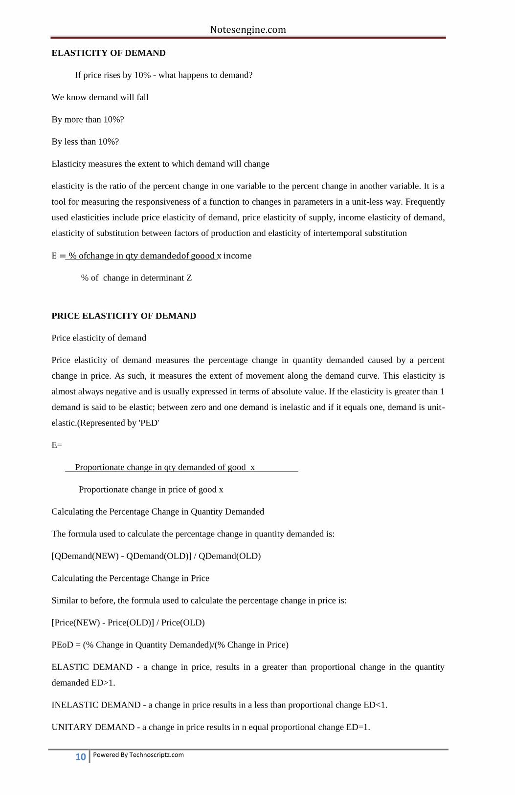
ZERO INCOME ELASTICITIES
This occurs when a change in income has NO effect on the demand for goods.
Notesengine.com
13 Powered By Technoscriptz.com
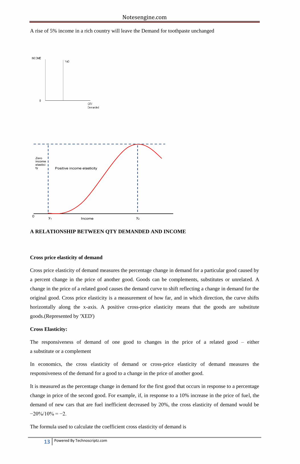
A rise of 5% income in a rich country will leave the Demand for toothpaste unchanged
A RELATIONSHIP BETWEEN QTY DEMANDED AND INCOME
Cross price elasticity of demand
Cross price elasticity of demand measures the percentage change in demand for a particular good caused by
a percent change in the price of another good. Goods can be complements, substitutes or unrelated. A
change in the price of a related good causes the demand curve to shift reflecting a change in demand for the
original good. Cross price elasticity is a measurement of how far, and in which direction, the curve shifts
horizontally along the x-axis. A positive cross-price elasticity means that the goods are substitute
goods.(Represented by 'XED')
Cross Elasticity:
The responsiveness of demand of one good to changes in the price of a related good – either
a substitute or a complement
In economics, the cross elasticity of demand or cross-price elasticity of demand measures the
responsiveness of the demand for a good to a change in the price of another good.
It is measured as the percentage change in demand for the first good that occurs in response to a percentage
change in price of the second good. For example, if, in response to a 10% increase in the price of fuel, the
demand of new cars that are fuel inefficient decreased by 20%, the cross elasticity of demand would be
−20%/10% = −2.
The formula used to calculate the coefficient cross elasticity of demand is

Notesengine.com
14 Powered By Technoscriptz.com
% of change in demand of one good
%of change in the price
TYPES OF CROSS ELASTICITY
NEGATIVE SUBSTITUTION ELASTICITY
the two goods, fuel and cars(consists of fuel consumption), are complements; that is, one is used with the
other. In these cases the cross elasticity of demand will be negative, as shown by the decrease in demand
for cars when the price of fuel increased.
INFINITE Substitution elasticity
Where the two goods are substitutes the cross elasticity of demand will be positive, so that as the price of
one goes up the demand of the other will increase. For example, in response to an increase in the price of
carbonated soft drinks, the demand for non-carbonated soft drinks will rise. In the case of perfect
substitutes, the cross elasticity of demand is equal to positive infinity.
ZERO SUBSTITUTION ELASTICITY
Where the two goods are independent, the cross elasticity of demand will be zero: as the price of one good
changes, there will be no change in demand for the other good.
DEMAND FORECASTING METHODS
There are several assumptions about forecasting:
1. There is no way to state what the future will be with complete certainty. Regardless of the methods that
we use there will always be an element of uncertainty until the forecast horizon has come to pass.
2. There will always be blind spots in forecasts. We cannot, for example, forecast completely new
technologies for which there are no existing paradigms.
3. Providing forecasts to policy-makers will help them formulate social policy. The new social policy, in
turn, will affect the future, thus changing the accuracy of the forecast.
OPINION POLLING METHODS
EXPERTS OPINION METHOD
Genius forecasting - This method is based on a combination of intuition, insight, and luck. Psychics and
crystal ball readers are the most extreme case of genius forecasting. Their forecasts are based exclusively
on intuition. Science fiction writers have sometimes described new technologies with uncanny accuracy
CONSUMER ‘S SURVEY METHOD
In this method consumer‘s are contacted personally to disclose their future plans
so that we can able to forecast the future because they are ultimate targeters/buyers
COMPLETE ENUMERATION SURVEY
Notesengine.com
15 Powered By Technoscriptz.com
Here all the units of consumers are taken into account without any cutshorts
So here large number of consumers will be there to get the unbiased information .The main
Advantage of this method is its accuracy and its main drawback is it is time consuming one.
SURVEY METHOD
Here from the total population certain number of units will be selected as sample units, then
the opinion collection will be made. This methopd is less tedious and less costly than the above method.
STATISTICAL METHODS
Fitting trend line by observation
This method of estimating trend is elementary,easy and quick.It involves merely plotting of
annual sales on graph and then estimating just by observation where the trend line lies.
Trend extrapolation - These methods examine trends and cycles in historical data, and then use
mathematical techniques to extrapolate to the future. The assumption of all these techniques is that the
forces responsible for creating the past, will continue to operate in the future. This is often a valid
assumption when forecasting short term horizons, but it falls short when creating medium and long term
forecasts. The further out we attempt to forecast, the less certain we become of the forecast
Simulation methods - Simulation methods involve using analogs to model complex systems. These
analogs can take on several forms. A mechanical analog might be a wind tunnel for modeling aircraft
performance. An equation to predict an economic measure would be a mathematical analog. A
metaphorical analog could involve using the growth of a bacteria colony to describe human population
growth. Game analogs are used where the interactions of the players are symbolic of social interactions
Trend Analysis: Uses linear and nonlinear regression with time as the explanatory variable, it is used
where pattern over time have a long-term trend. Unlike most time-series forecasting techniques, the Trend
Analysis does not assume the condition of equally spaced time series.
Nonlinear regression does not assume a linear relationship between variables. It is frequently used when
time is the independent variable.
Simple Moving Averages: The best-known forecasting methods is the moving averages or simply takes a
certain number of past periods and add them together; then divide by the number of periods. Simple
Moving Averages (MA) is effective and efficient approach provided the time series is stationary in both
mean and variance. The following formula is used in finding the moving average of order n, MA(n) for a
period t+1,
Exponential Smoothing Techniques: One of the most successful forecasting methods is the exponential
smoothing (ES) techniques. Moreover, it can be modified efficiently to use effectively for time series with
seasonal patterns. It is also easy to adjust for past errors-easy to prepare follow-on forecasts, ideal for
situations where many forecasts must be prepared, several different forms are used depending on presence
of trend or cyclical variations. In short, an ES is an averaging technique that uses unequal weights;
however, the weights applied to past observations decline in an exponential manner
Notesengine.com
16 Powered By Technoscriptz.com
Smoothing techniques are used to reduce irregularities (random fluctuations) in time series data. They
provide a clearer view of the true underlying behavior of the series. Moving averages rank among the most
popular techniques for the preprocessing of time series. They are used to filter random "white noise" from
the data, to make the time series smoother or even to emphasize certain informational components
contained in the time series.
Exponential smoothing is a very popular scheme to produce a smoothed time series. Whereas in moving
averages the past observations are weighted equally, Exponential Smoothing assigns exponentially
decreasing weights as the observation get older. In other words, recent observations are given relatively
more weight in forecasting than the older observations. Double exponential smoothing is better at handling
trends. Triple Exponential Smoothing is better at handling parabola trends.
Least-Squares Method: To predict the mean y-value for a given x-value, we need a line which passes
through the mean value of both x and y and which minimizes the sum of the distance between each of the
points and the predictive line. Such an approach should result in a line which we can call a "best fit" to the
sample data. The least-squares method achieves this result by calculating the minimum average squared
deviations between the sample y points and the estimated line. A procedure is used for finding the values of
a and b which reduces to the solution of simultaneous linear equations. Shortcut formulas have been
developed as an alternative to the solution of simultaneous equations..
Regression and Moving Average: When a time series is not a straight line one may use the moving
average (MA) and break-up the time series into several intervals with common straight line with positive
trends to achieve linearity for the whole time series. The process involves transformation based on slope
and then a moving average within that interval. For most business time series, one the following
transformations might be effective
ARIMA METHOD
A couple of notes on this model.
The Box-Jenkins model assumes that the time series is stationary. Box and Jenkins recommend
differencing non-stationary series one or more times to achieve stationarity. Doing so produces an ARIMA
model, with the "I" standing for "Integrated".
Some formulations transform the series by subtracting the mean of the series from each data point. This
yields a series with a mean of zero. Whether you need to do this or not is dependent on the software you
use to estimate the model.
Box-Jenkins models can be extended to include seasonal autoregressive and seasonal moving average
terms. Although this complicates the notation and mathematics of the model, the underlying concepts for
seasonal autoregressive and seasonal moving average terms are similar to the non-seasonal autoregressive
and moving average terms.
The most general Box-Jenkins model includes difference operators, autoregressive terms, moving average
terms, seasonal difference operators, seasonal autoregressive terms, and seasonal moving average terms. As
with modeling in general, however, only necessary terms should be included in the model
There are five stages of analysis in this method:
Removal of trend
Model identification
Notesengine.com
17 Powered By Technoscriptz.com
Parameter estimation
Verification
Forecasting
MEANING OF SUPPLY
What is Supply?
Supply is the quantity of a good or service a firm is willing to produce at all prices.
What is the law of Supply?
If nothing else changes, firms are willing to supply a greater quantity of good or service at higher prices
than lower.
Determinants of Supply
Productivity (Improvements in machines and production processes of a good or service)
Inputs ( Change in the price of inputs required to produce the good or service.)
Government Actions (Subsidies, Taxes and Regulations)
Technology (Improvements in machines and production processes of a good or service)
Outputs ( Price changes in other products produced by the firm)
Expectations (outlook of future prices and profits)
Size of Industry (Number of firms
Change in the number of suppliers
Any factor that increases the cost of production decreases supply.
Any factor that decreases the cost of production increases supply.
SUPPLY FUNCTION
Sx = f(Px,Py, Pz,……..;Pf ,O,T)
Sx=Amount supplied of good x
Px= Price of good X
Py,Pz= Prices of other goods in the market
Pf = Prices of factors of production
O = objective of the producer
T = State of technology used by the producer to produce good x
Elasticity of supply
Responsiveness of producers to changes in the price of their goods or services. As a general rule, if prices
rise so does the supply.

Notesengine.com
18 Powered By Technoscriptz.com
Elasticity of supply is measured as the ratio of proportionate change in the quantity supplied to the
proportionate change in price. High elasticity indicates the supply is sensitive to changes in prices, low
elasticity indicates little sensitivity to price changes, and no elasticity means no relationship with price.
Also called price elasticity of supply.
Price elasticity of supply measures the relationship between change in quantity supplied and a change in
price. The formula for price elasticity of supply is:
Percentage change in quantity supplied / Percentage change in price
The value of elasticity of supply is positive, because an increase in price is likely to increase the quantity
supplied to the market and vice versa.
FACTORS THAT DETERMINE ELASTICITY OF SUPPLY
The elasticity of supply depends on the following factors
The value of price elasticity of supply is positive, because an increase in price is likely to increase the
quantity supplied to the market and vice versa. The elasticity of supply depends on the following factors:
SPARE CAPACITY
How much spare capacity a firm has - if there is plenty of spare capacity, the firm should be able to
increase output quite quickly without a rise in costs and therefore supply will be elastic
STOCKS
The level of stocks or inventories - if stocks of raw materials, components and finished products are high
then the firm is able to respond to a change in demand quickly by supplying these stocks onto the market -
supply will be elastic
EASE OF FACTOR SUBSTITUTION
Consider the sudden and dramatic increase in demand for petrol canisters during the recent fuel shortage.
Could manufacturers of cool-boxes or producers of other types of canister have switched their production
processes quickly and easily to meet the high demand for fuel containers?
Notesengine.com
19 Powered By Technoscriptz.com
If capital and labour resources are occupationally mobile then the elasticity of supply for a product is likely
to be higher than if capital equipment and labour cannot easily be switched and the production process is
fairly inflexible in response to changes in the pattern of demand for goods and services.
TIME PERIOD
Supply is likely to be more elastic, the longer the time period a firm has to adjust its production. In the short
run, the firm may not be able to change its factor inputs. In some agricultural industries the supply is fixed
and determined by planting decisions made months before, and climatic conditions, which affect the
production, yield.
Economists sometimes refer to the momentary time period - a time period that is short enough for supply to
be fixed i.e. supply cannot respond at all to a change in demand.
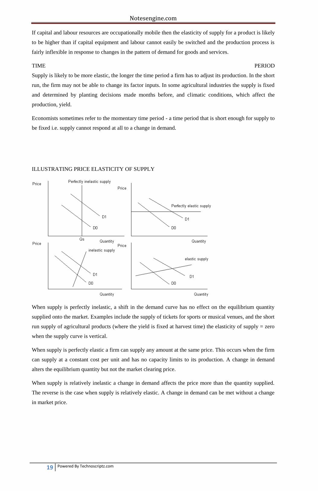
ILLUSTRATING PRICE ELASTICITY OF SUPPLY
When supply is perfectly inelastic, a shift in the demand curve has no effect on the equilibrium quantity
supplied onto the market. Examples include the supply of tickets for sports or musical venues, and the short
run supply of agricultural products (where the yield is fixed at harvest time) the elasticity of supply = zero
when the supply curve is vertical.
When supply is perfectly elastic a firm can supply any amount at the same price. This occurs when the firm
can supply at a constant cost per unit and has no capacity limits to its production. A change in demand
alters the equilibrium quantity but not the market clearing price.
When supply is relatively inelastic a change in demand affects the price more than the quantity supplied.
The reverse is the case when supply is relatively elastic. A change in demand can be met without a change
in market price.

Notesengine.com
20 Powered By Technoscriptz.com
UNIT-III
PRODUCTION FUNCTION AND COST ANAYSIS
Production Function – Returns of Scale – Production optimization – Least cost output – isoquants –
Managerial uses of production function. Cost concepts – Cost function – Types of cost –
Determinants of cost – Short run and Long run cost curves – Cost output Decision – Estimation of
Cost.
A production function is a function that specifies the output of a firm, an industry, or an entire economy for
all combinations of inputs. This function is an assumed technological relationship, based on the current
state of engineering.
CONCEPT OF PRODUCTION FUNCTION
The production function relates the output of a firm to the amount of inputs, typically capital and
labor
In a general mathematical form, a production function can be expressed as:
Q = f(X1,X2,X3,...,Xn)
where:
Q = quantity of output

Notesengine.com
21 Powered By Technoscriptz.com
X1,X2,X3,...,Xn = quantities of factor inputs (such as capital, labour, land or raw materials). This general
form does not encompass joint production; that is a production process that has multiple co-products or
outputs
COBB-DOUGLAS PRODUCTION FUNCTION
A standard production function which is applied to describe much output two inputs into a production
process make. It is used commonly in both macro and micro examples.
For capital K, labor input L, and constants a, b, and c, the Cobb-Douglas production function is:
f(k,n) = bkanc
If a+c=1 this production function has constant returns to scale. (Equivalently, in mathematical language, it
would then be linearly homogenous.) This is a standard case and one often writes (1-a) in place of c.
Log-linearization simplifies the function, meaning just that taking logs of both sides of a Cobb-Douglass
function gives one better separation of the components.
In the Cobb-Douglass function the elasticity of substitution between capital and labor is 1 for all values of
capital and labor
STAGES IN PRODUCTION FUNCTION
To simplify the interpretation of a production function, it is common to divide its range into 3 stages. In
Stage 1 (from the origin to point B) the variable input is being used with increasing output per unit, the
latter reaching a maximum at point B (since the average physical product is at its maximum at that point).
Because the output per unit of the variable input is improving throughout stage 1, a price-taking firm will
always operate beyond this stage.
In Stage 2, output increases at a decreasing rate, and the average and marginal physical product are
declining. However the average product of fixed inputs (not shown) is still rising, because output is rising
while fixed input usage is constant. In this stage, the employment of additional variable inputs increases the
output per unit of fixed input but decreases the output per unit of the variable input. The optimum
input/output combination for the price-taking firm will be in stage 2, although a firm facing a downward-
sloped demand curve might find it most profitable to operate in Stage 1. In Stage 3, too much variable input
is being used relative to the available fixed inputs: variable inputs are over-utilized in the sense that their
presence on the margin obstructs the production process rather than enhancing it. The output per unit of
both the fixed and the variable input declines throughout this stage. At the boundary between stage 2 and
stage 3, the highest possible output is being obtained from the fixed input
Notesengine.com
22 Powered By Technoscriptz.com
RETURNS TO SCALE
In production, returns to scale refers to changes in output subsequent to a proportional change in all inputs
(where all inputs increase by a constant factor). If output increases by that same proportional change then
there are constant returns to scale (CRTS). If output increases by less than that proportional change, there
are decreasing returns to scale (DRS). If output increases by more than that proportion, there are increasing
returns to scale (IRS)
Short example: where all inputs increase by a factor of 2, new values for output should be:
Twice the previous output given = a constant return to scale (CRTS)
Less than twice the previous output given = a decreased return to scale (DRS)
More than twice the previous output given = an increased return to scale (IRS)
when we increase all inputs by a multiplier of m. Suppose our inputs are capital or labor, and we double
each of these (m = 2), we want to know if our output will more than double, less than double, or exactly
double. This leads to the following definitions:
Increasing Returns to Scale
When our inputs are increased by m, our output increases by more than m.
Constant Returns to Scale
When our inputs are increased by m, our output increases by exactly m.
Decreasing Returns to Scale
When our inputs are increased by m, our output increases by less than m.
Our multiplier must always be positive, and greater than 1, since we want to look at what happens when we
increase production. An m of 1.1 indicates that we've increased our inputs by 10% and an m of 3 indicates
that we've tripled the amount of inputs we use. Now we will look at a few production functions and see if
we have increasing, decreasing, or constant returns to scale. Note that some textbooks use Q for quantity in
the production function, and others use Y for output. It does not change this analysis any, so use whatever
your professor uses
� Opportunity cost = economic cost
Cost is foregone benefit of a resource in it‘s best alternative use
Cost = market price only when price reflects value of marginal product (perfect competition)
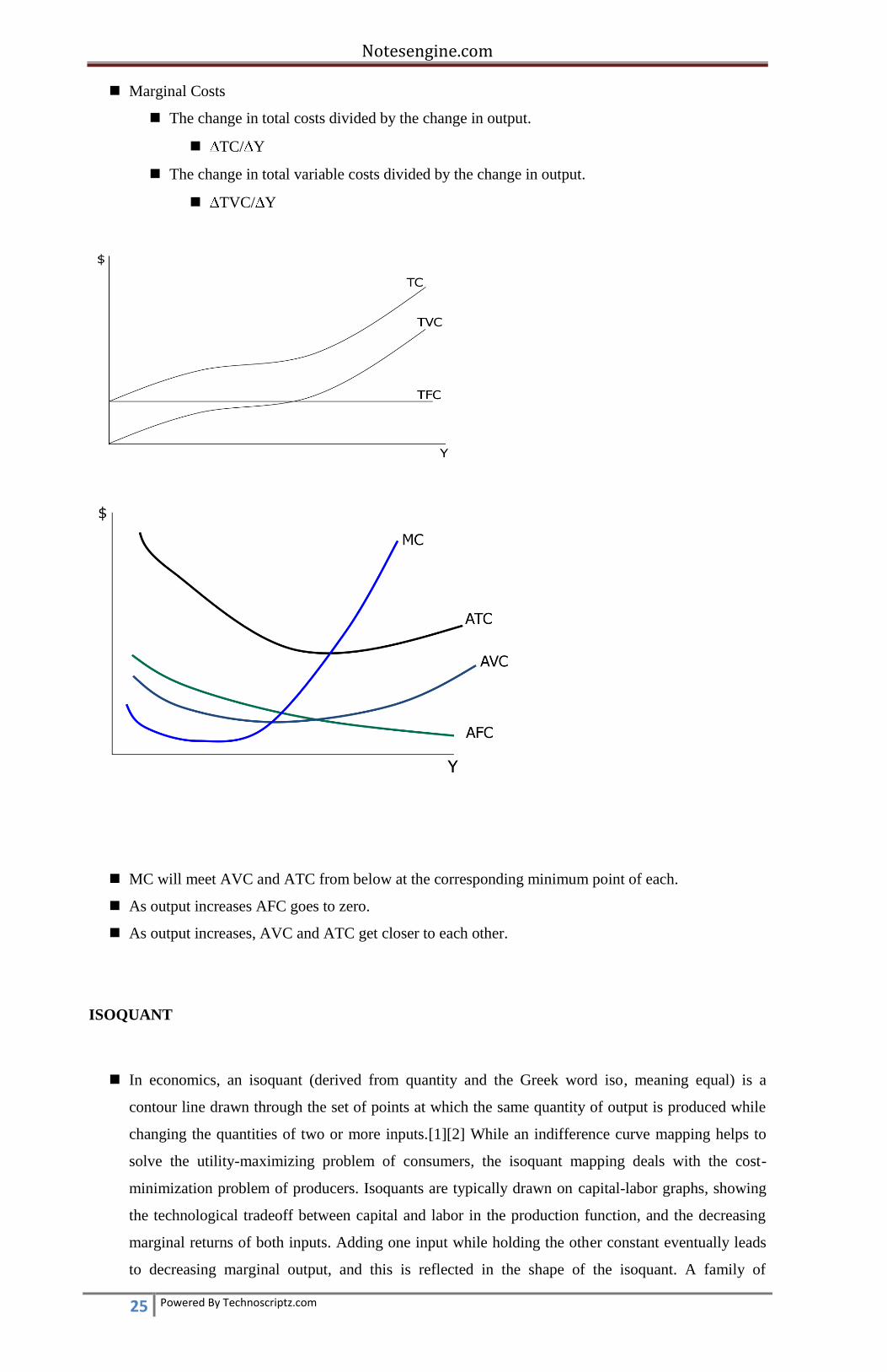
Fixed costs
do not change when the quantity of output produced Changes
These cost exist whether production occurs or not.
In the long-run there are no fixed costs.
Can be both cash and non-cash expenses.

Notesengine.com
23 Powered By Technoscriptz.com
E.g., depreciation on tractors and buildings, etc.
Variable Costs
These costs exist only if production occurs.
E.g., fuel for tractor, seed, etc.
Total Fixed Costs (TFC)
The summation of all fixed and sunk costs to production.
Total Variable Costs (TVC)
The summation of all variable costs to production.
Total Costs (TC)
The summation of total fixed and total variable costs.
TC=TFC+TVC
Accounting or actual costs
The total amount of money or goods expended in an endeavour. It is money paid out at some time in the
past and recorded in journal entries and ledgers.
Opportunity Costs
The value of the product not produced because an input was used for another purpose.
The income that would have been received if the input had been used in its most profitable
alternative use.
It denotes the real cost of using an input.
Sunk Costs
Is an expenditure that cannot be recovered.
In essence, it becomes part of fixed costs.
E.g., pre-harvest costs.
Transaction cost
a transaction cost is a cost incurred in making an economic exchange (restated: the cost of
participating in a market). For example, most people, when buying or selling a stock, must pay a
commission to their broker
Short run costs vs long run costs
The short run is a period of time sufficiently short that only some of the variables can be changed.
In the short-run, there are many ways to choose how to produce.
Maximize output.
Utility maximization of the manager.
Profit maximization.
Notesengine.com
24 Powered By Technoscriptz.com
Profit ( ) is defined as total revenue minus total cost, i.e., = TR – TC.
When examining output, we want to set our production level where MR = MC when MR > AVC in
the short-run.
If MR AVC, we would want to shut down.
Why?
If we can not set MR exactly equal to MC, we want to produce at a level where MR is as close as
possible to MC, where MR > MC.
Suppose MR < MC.
This implies that by producing more output, you have a greater addition of cost than you do revenue.
Hence you would not make the change.
Suppose MR > MC.
This implies that by producing more output, you have a greater addition of revenue than you do cost.
Hence you would make the change.
You would stop increasing output at the point where the trade-off in additional revenue is just equal
to the trade-off in additional costs.
The long run is a period of time that all variables can be changed.
To maximize profits, the farmer should produce when selling price is greater than ATC at the
production level where MC = MR.
To minimize losses, the farmer should not produce when selling price is less than ATC, i.e.,
shutdown the business.
The long run average cost (LRAC) curve is the envelope of the short run average cost curves when
the size of the operation is allowed to increase or decrease.
Note that a short run average cost curve exists for every possible farm size, as defined by the amount
of fixed input available.
In a competitive market, the long run optimal production will occur at the lowest point on the LRAC,
i.e., economic profits are driven to zero
A measure of size in the long run between output and costs as farm size increases (EOS) is the
following:
EOS = percent change in costs divided by percent change in output value
If this ratio of EOS is less than one, then there are decreasing costs to expanding production, i.e.,
increasing returns to size.
If this ratio is equal to one, then there are constant costs to expanding production, i.e., constant
returns to size.
If this ratio is greater than one, then there are increasing costs to expanding production, i.e.,
decreasing returns to size.
Average Fixed Costs (AFC)
The total fixed costs divided by output.
Average Variable Costs (AVC)
The total variable costs divided by output.
Average Total Costs (ATC)
The total costs divided by output.
The summation of average fixed costs and average variable costs, i.e., ATC=AFC+AVC
Notesengine.com
25 Powered By Technoscriptz.com
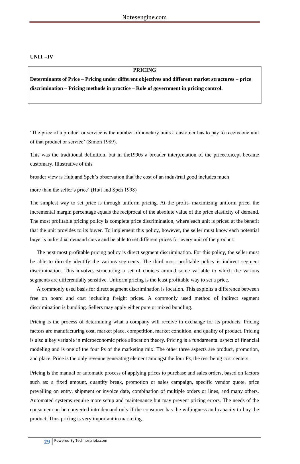
Marginal Costs
The change in total costs divided by the change in output.
TC/ Y
The change in total variable costs divided by the change in output.
TVC/ Y
MC will meet AVC and ATC from below at the corresponding minimum point of each.
As output increases AFC goes to zero.
As output increases, AVC and ATC get closer to each other.
ISOQUANT
In economics, an isoquant (derived from quantity and the Greek word iso, meaning equal) is a
contour line drawn through the set of points at which the same quantity of output is produced while
changing the quantities of two or more inputs.[1][2] While an indifference curve mapping helps to
solve the utility-maximizing problem of consumers, the isoquant mapping deals with the cost-
minimization problem of producers. Isoquants are typically drawn on capital-labor graphs, showing
the technological tradeoff between capital and labor in the production function, and the decreasing
marginal returns of both inputs. Adding one input while holding the other constant eventually leads
to decreasing marginal output, and this is reflected in the shape of the isoquant. A family of

Notesengine.com
26 Powered By Technoscriptz.com
isoquants can be represented by an isoquant map, a graph combining a number of isoquants, each
representing a different quantity of output. Isoquants are also called equal product curves.
An isoquant shows the extent to which the firm in question has the ability to substitute between the
two different inputs at will in order to produce the same level of output. An isoquant map can also
indicate decreasing or increasing returns to scale based on increasing or decreasing distances
between the isoquant pairs of fixed output increment,as you increase output. If the distance between
those isoquants increases as output increases, the firm's production function is exhibiting decreasing
returns to scale; doubling both inputs will result in placement on an isoquant with less than double
the output of the previous isoquant. Conversely, if the distance is decreasing as output increases, the
firm is experiencing increasing returns to scale; doubling both inputs results in placement on an
isoquant with more than twice the output of the original isoquant.
As with indifference curves, two isoquants can never cross. Also, every possible combination of
inputs is on an isoquant. Finally, any combination of inputs above or to the right of an isoquant
results in more output than any point on the isoquant. Although the marginal product of an input
decreases as you increase the quantity of the input while holding all other inputs constant, the
marginal product is never negative in the empirically observed range since a rational firm would
never increase an input to decrease output.
SHORT RUN AND LONG RUN COST CURVES

Notesengine.com
27 Powered By Technoscriptz.com
short-run cost curves are normally based on a production function with one variable factor of
production that displays first increasing and then decreasing marginal productivity. Increasing
marginal productivity is associated with the negatively sloped portion of the marginal cost
curve,while decreasing marginal productivity is associated with the positively sloped portion.
Theaverage fixed cost (AFC) curve is the cost of the fixed factor of production divided by
thequantity of units of the output, while the average variable cost (AVC) curve cost traces out theper
unit cost of variable factor of production. The U-shaped average total cost (ATC) curve isderived by
adding the average fixed and variable costs. The marginal cost (MC) intersects both the AVC and
ATC curves at their minimum points. Declining average total costs are explained as the result of
spreading the fixed costs over greater quantities and, at low quantities, the result of the increasing
marginal productivity, in addition. Increasing average costs occur when the effect of declining
marginal productivity overwhelms the effect of spreading the fixed costs.
The long-run cost curves, usually presented in a separate diagram, are also expressed most
commonly in their average, or per unit, form, represented here in Figure 2. The long-run average cost
(LRAC) curve is shown to be an envelope of the short-run average cost (SRAC) curves, lying
everywhere below or tangent to the short-run curves. The firm is constrained in the shortrun in
selecting the optimal mix of factors of production and so will never be able to find a cheaper mix
than can be found in the long-run when there are no constraints. If there are a discrete number of
plant sizes available, the LRAC will be the scalloped curve obtained by joining those parts of the
SRAC curves that represent the lowest cost of production for a given quantity.

Notesengine.com
28 Powered By Technoscriptz.com
Notesengine.com
29 Powered By Technoscriptz.com
UNIT –IV
PRICING
Determinants of Price – Pricing under different objectives and different market structures – price
discrimination – Pricing methods in practice – Role of government in pricing control.
‗The price of a product or service is the number ofmonetary units a customer has to pay to receiveone unit
of that product or service‘ (Simon 1989).
This was the traditional definition, but in the1990s a broader interpretation of the priceconcept became
customary. Illustrative of this
broader view is Hutt and Speh‘s observation that‗the cost of an industrial good includes much
more than the seller‘s price‘ (Hutt and Speh 1998)
The simplest way to set price is through uniform pricing. At the profit- maximizing uniform price, the
incremental margin percentage equals the reciprocal of the absolute value of the price elasticity of demand.
The most profitable pricing policy is complete price discrimination, where each unit is priced at the benefit
that the unit provides to its buyer. To implement this policy, however, the seller must know each potential
buyer‘s individual demand curve and be able to set different prices for every unit of the product.
The next most profitable pricing policy is direct segment discrimination. For this policy, the seller must
be able to directly identify the various segments. The third most profitable policy is indirect segment
discrimination. This involves structuring a set of choices around some variable to which the various
segments are differentially sensitive. Uniform pricing is the least profitable way to set a price.
A commonly used basis for direct segment discrimination is location. This exploits a difference between
free on board and cost including freight prices. A commonly used method of indirect segment
discrimination is bundling. Sellers may apply either pure or mixed bundling.
Pricing is the process of determining what a company will receive in exchange for its products. Pricing
factors are manufacturing cost, market place, competition, market condition, and quality of product. Pricing
is also a key variable in microeconomic price allocation theory. Pricing is a fundamental aspect of financial
modeling and is one of the four Ps of the marketing mix. The other three aspects are product, promotion,
and place. Price is the only revenue generating element amongst the four Ps, the rest being cost centers.
Pricing is the manual or automatic process of applying prices to purchase and sales orders, based on factors
such as: a fixed amount, quantity break, promotion or sales campaign, specific vendor quote, price
prevailing on entry, shipment or invoice date, combination of multiple orders or lines, and many others.
Automated systems require more setup and maintenance but may prevent pricing errors. The needs of the
consumer can be converted into demand only if the consumer has the willingness and capacity to buy the
product. Thus pricing is very important in marketing.

Notesengine.com
30 Powered By Technoscriptz.com
Transfer pricing refers to the pricing of contributions (assets, tangible and intangible, services, and funds)
transferred within an organization (a corporation or similar entity). For example, goods from the production
division may be sold to the marketing division, or goods from a parent company may be sold to a foreign
subsidiary. Since the prices are set within an organization (i.e. controlled),
Cost plus pricing method
The Cost Plus (CP) method, generally used for the trade of finished goods, is determined by adding an
appropriate markup to the costs incurred by the selling party in manufacturing/purchasing the goods or
services provided, with the appropriate markup being based on the profits of other companies comparable
to the tested party. For example, the arm's length price for a transaction involving the sale of finished
clothing to a related distributor would be determined by adding an appropriate markup to the cost of
materials, labour, manufacturing, and so on.
Price skimming is a pricing strategy in which a marketer sets a relatively high price for a product or
service at first, then lowers the price over time. It is a temporal version of price discrimination/yield
management. It allows the firm to recover its sunk costs quickly before competition steps in and lowers the
market price.
Price skimming is sometimes referred to as riding down the demand curve. The objective of a price
skimming strategy is to capture the consumer surplus. If this is done successfully, then theoretically no
customer will pay less for the product than the maximum they are willing to pay. In practice, it is almost
impossible for a firm to capture all of this surplus.
Cost-plus pricing is a pricing method used by companies. It is used primarily because it is easy to
calculate and requires little information. There are several varieties, but the common thread in all of them is
that one first calculates the cost of the product, then includes an additional amount to represent profit. It is a
way for companies to calculate how much profit they will make. Cost-plus pricing is often used on
government contracts, and has been criticized as promoting wasteful expenditures.
The method determines the price of a product or service that uses direct costs, indirect costs, and fixed
costs whether related to the production and sale of the product or service or not. These costs are converted
to per unit costs for the product and then a predetermined percentage of these costs is added to provide a
profit margin
Target rate of return pricing is a pricing method used almost exclusively by market leaders or
monopolists. You start with a rate of return objective, like 5% of invested capital, or 10% of sales revenue.
Then you arrange your price structure so as to achieve these target rates of return.[1]
For example, assume a firm invests $100 million in order to produce and market designer snowflakes, and
they estimate that with demand for designer snowflakes being what it is, they can sell 2 million flakes per
year.
Joint Products are two or more products, produced from the same process or operation, considered to be of
relative equal importance. Pricing for joint products is a little more complex than pricing for a single
product. To begin with there are two demand curves. The characteristics of each demand curve could be
different. Demand for one product could be greater than for the other product. Consumers of one product
Notesengine.com
31 Powered By Technoscriptz.com
could be more price elastic than the consumers of the other product (and therefore more sensitive to
changes in the product's price).
Dual pricing
Even within a country, differentiated pricing may be established to ensure that citizens receive lower prices
than non-citizens; this is known as dual pricing. This is particularly common for goods that are subsidized
or otherwise provided by the state (and hence paid by taxpayers). Thus Finns, Thais, and Indians (among
others) may purchase special fare tickets for public transportation that are available only to citizens. Many
countries also maintain separate admission charges for museums, national parks and similar facilities, the
usually professed rationale being that citizens should be able to educate themselves and enjoy the country's
natural wonders cheaply, but other visitors should pay the market rate
Premium pricing
For certain products, premium products are priced at a level (compared to "regular" or "economy"
products) that is well beyond their marginal cost of production. For example, a coffee chain may price
regular coffee at $1, but "premium" coffee at $2.50 (where the respective costs of production may be $0.90
and $1.25).
A market economy is economy based on the power of division of labor in which the prices of goods and
services are determined in a free price system set by supply and demand.[1]
This is often contrasted with a planned economy, in which a central government determines the price of
goods and services using a fixed price system. Market economies are also contrasted with mixed economy
where the price system is not entirely free but under some government control or heavily regulated, which
is sometimes combined with state-led economic planning that is not extensive enough to constitute a
planned economy.
In the real world, market economies do not exist in pure form, as societies and governments regulate them
to varying degrees rather than allow self-regulation by market forces.[2][3] The term free-market economy
is sometimes used synonymously with market economy,[4] but, as Ludwig Erhard once pointed out, this
does not preclude an economy from having socialist attributes opposed to a laissez-faire system.[5]
Economist Ludwig von Mises also pointed out that a market economy is still a market economy even if the
government intervenes in pricing.[6]
Different perspectives exist as to how strong a role the government should have in both guiding the market
economy and addressing the inequalities the market produces. For example, there is no universal agreement
on issues such as central banking, and welfare. However, most economists oppose protectionist tariffs.[7]
The term market economy is not identical to capitalism where a corporation hires workers as a labour
commodity to produce material wealth and boost shareholder profits.[8] Market mechanisms have been
utilized in a handful of socialist states, such as China, Yugoslavia and even Cuba to a very limited extent.
It is also possible to envision an economic system based on independent producers, cooperative, democratic
worker ownership and market allocation of final goods and services; the labour-managed market economy
is one of several proposed forms of market socialism.[9]

Notesengine.com
32 Powered By Technoscriptz.com
1.Uniform pricing.
(a) Uniform pricing: a pricing policy where a seller charges the same price
for every unit of the product.
2. Profit maximizing price (incremental margin percentage rule):
A price where the incremental margin percentage (i.e., price lessmarginal cost divided by the price)
is equal to the reciprocal of the absolute value of the price elasticity of demand. This is the rule ofmarginal
revenue equals the marginal cost.
i. Price elasticity may very along a demand curve, marginal cost changes with scale of production. The above
proceduretypically involves a series of trials and errors with different
prices.
ii. Intuitive factors that underlie price elasticity: direct and indirect substitutes, buyers‘ prior commitments,
search cost.
(c)Price adjustments following changes in demand and cost. i. To maximize profits, a seller should consider
both demand and costs.
ii. A seller should adjust its price to changes in either the price elasticity or the marginal cost.
iii. It must consider the effect of the price change on the quantity demanded.
iv. If demand ismore elastic (price elasticity will be a largernegative number), the seller should aim for a
lower incrementalmargin percentage, and not necessarily a lower price, andlikewise,
v. If demand isless elastic, the seller should aim for a higherincremental margin percentage, and not
necessarily a higherprice.
vi. A seller should not necessarily adjust the price by the same amount as a change in marginal cost.
(d) Special notes.
i. Only the incremental margin percentage (i.e., price less marginal cost divided by the price) is relevant to
pricing.
(1). Contribution margin percentage (i.e., price less averagevariable cost divided by the price) is not relevant to
pricing.
(2). Variable costs may increase or decrease with the scale of production, and hence, marginal cost will not be
the same as average variable cost.
ii. Setting price by simply marking up average cost will not maximize profit. Problems of cost plus pricing:
(1). In businesses with economies of scale, average cost depends on scale, but scale depends on price. It is a
circular exercise.
(2). Cost plus pricing gives no guidance as to the markup on average cost.
(e)Limitations of uniform pricing (incremental margin percentage rule).
i. The inframarginal buyers do not pay as much as they will be
willing to pay. A seller could increase its profit by taking some
of the buyer surplus
In economics, market structure (also known as the number of firms producing identical products.)
Monopolistic competition, also called competitive market, where there are a small number of
dependent firms which each have a very large proportion of the market share and products from
different companies are different.
Notesengine.com
33 Powered By Technoscriptz.com
Oligopoly, in which a market is dominated by a small number of firms which own more than 40% of
the market share.
Oligopsony, a market, where many sellers can be present but meet only a few buyers.
Monopoly, where there is only one provider of a product or service.
Natural monopoly, a monopoly in which economies of scale cause efficiency to increase
continuously with the size of the firm. A firm is a natural monopoly if it is able to serve the entire
market demand at a lower cost than any combination of two or more smaller, more specialized firms.
Monopsony, when there is only one buyer in a market.
The imperfectly competitive structure is quite identical to the realistic market conditions where some
monopolistic competitors, monopolists, oligopolists, and duopolists exist and dominate the market
conditions. The elements of Market Structure include the number and size distribution of firms, entry
conditions, and the extent of differentiation.
These somewhat abstract concerns tend to determine some but not all details of a specific concrete market
system where buyers and sellers actually meet and commit to trade. Competition is useful because it reveals
actual customer demand and induces the seller (operator) to provide service quality levels and price levels
that buyers (customers) want, typically subject to the seller‘s financial need to cover its costs. In other
words, competition can align the seller‘s interests with the buyer‘s interests and can cause the seller to
reveal his true costs and other private information. In the absence of perfect competition, three basic
approaches can be adopted to deal with problems related to the control of market power and an asymmetry
between the government and the operator with respect to objectives and information: (a) subjecting the
operator to competitive pressures, (b) gathering information on the operator and the market, and (c)
applying incentive regulation.[1]
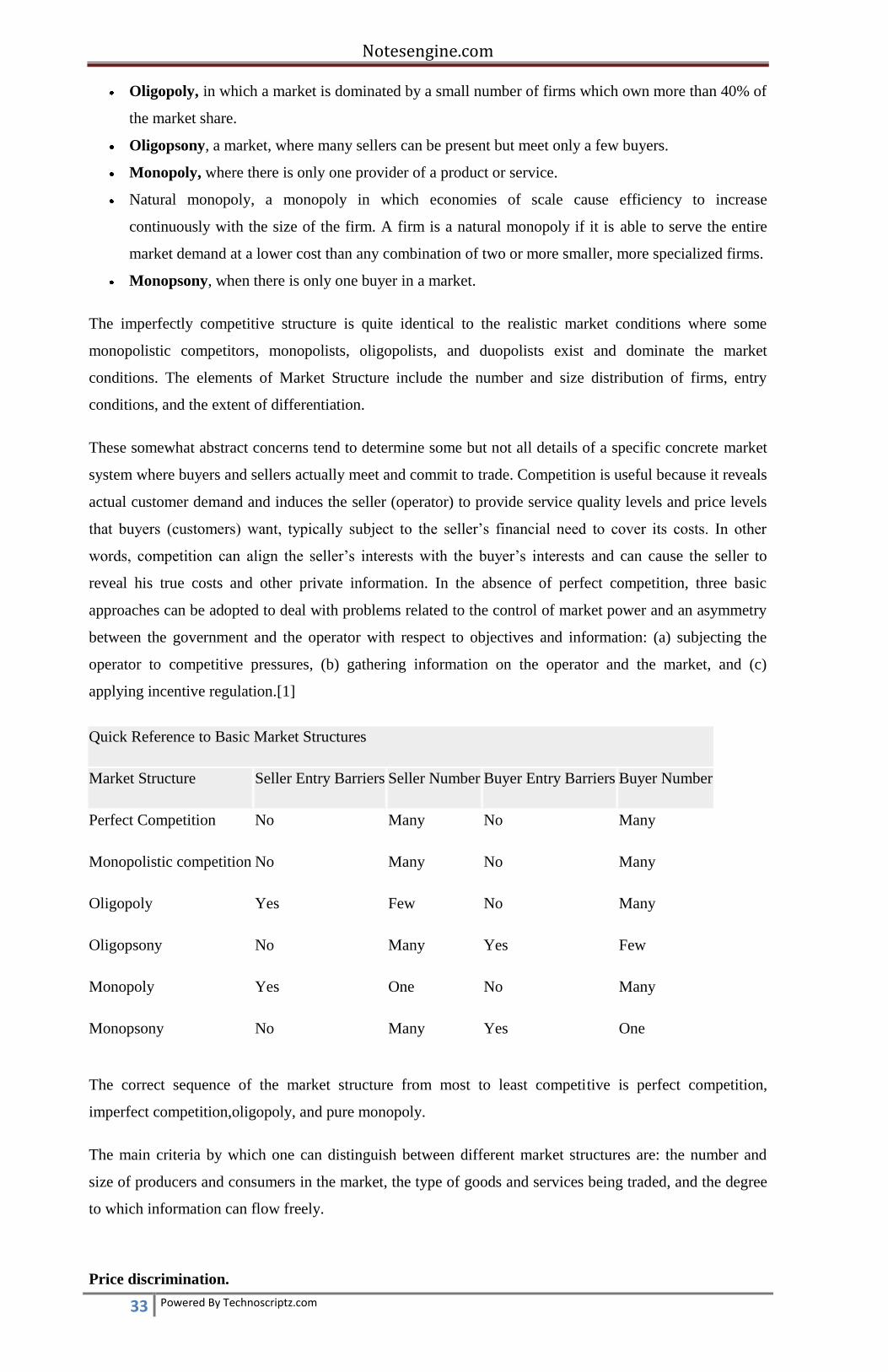
Quick Reference to Basic Market Structures
Market Structure Seller Entry Barriers Seller Number Buyer Entry Barriers Buyer Number
Perfect Competition No Many No Many
Monopolistic competition No Many No Many
Oligopoly Yes Few No Many
Oligopsony No Many Yes Few
Monopoly Yes One No Many
Monopsony No Many Yes One
The correct sequence of the market structure from most to least competitive is perfect competition,
imperfect competition,oligopoly, and pure monopoly.
The main criteria by which one can distinguish between different market structures are: the number and
size of producers and consumers in the market, the type of goods and services being traded, and the degree
to which information can flow freely.
Price discrimination.

Notesengine.com
34 Powered By Technoscriptz.com
Pricing policy where a seller sets different incremental margins on various units of the same or similar
product.
(a) To earn a higher incremental margin from buyers with higher benefit,and a smaller margin from buyers
with lower benefit.
Complete price discrimination: the pricing policy where a seller prices each unit of output at the buyer‘s
benefit and sells a quantity where the marginal benefit equals the marginal cost.
(a) All the buyer surplus is extracted. Every buyer is charged the maximum she is willing for pay for each
unit.
(b) Economically efficient quantity: all the opportunity for additional profit through changes in sales is
exploited.
(c) Extracts a higher price for units that would be sold under uniform pricing and extends sales by selling
additional units that would not be sold.
Reasons Price Discrimination
• Occurs when different net prices are charged for the same good
– Suppose consumers differ in their distance from the point of sale: If differences in prices exactly reflect
transport costs, prices are not discriminatory
– Suppose consumers buy nearly identical variants of the same basic good. If the difference in price
between
variants exactly equals the cost of characteristics that are in one but not the other, prices are not
discriminatory
First Degree Price Discrimination
• Every consumer pays his own reservation price
Marginal Revenue = Average Revenue
– Most profitable type of pricing
– Same quantity is sold as in competition
• Possible examples: small town doctor, shoe
repair shop, piano teacher
Valuebased more than cost based pricing often helps build profits.
•Firms charge different customers different prices, which is known as price discrimination.
This chapter also looks at pricing within a firm called transfer pricing.
•Pricing techniques that are used by many multi product firms, such as fullcost pricing and target return
pricing
Second Degree Price Discrimination
• Consumers distinguished by the quantity of the good they consume
– Quantity discounts
– Two‐ part tariffs
• Examples: software site licenses, toothpaste
Third Degree Price Discrimination
• Consumers are divided into groups or market segments according to some observable characteristic, and
each is charged a different price

Notesengine.com
35 Powered By Technoscriptz.com
– Higher price is given to buyers with less elastic demand
• Examples: airlines, student and senior
discounts
some pricing strategies for Smart Marketers.
Price-lining:
Price-lining features products at a limited number of prices, reflecting varying product quality or product
lines. This strategy can help smart marketers sell top quality produce at a premium price and an ―economy
line‖, e.g., overripe or smaller fruits. Price-lining can also make shopping easier for consumers and sellers
because
there are fewer prices to consider and handle.
Single-pricing:
The single-price strategy charges customers the same price for all items. Items are packaged in different
volumes based on the single price for which they would be sold. With such a policy the variety of offerings
is often limited. The strength is being able to avoid employee error and facilitate the speed of transactions.
Also,
customers know what to expect. There are no surprises for customers.
Loss-leader pricing: A less-than-normal markup or margin on an item is taken to
increase customer traffic. The loss-leaders should be well-known, frequently purchased
items. The idea is that customers will come to buy the ―leaders‖ and will also purchase
regularly priced items. If customers only buy the ―loss leaders,‖ the marketer is in
trouble.
Odd-ending pricing: Odd-ending prices are set just below the dollar figure, such as $1.99
a pound instead of $2.00. Some believe that consumers perceive odd-ending prices to be
substantially lower than prices with even-ending. However, it might not be suitable in
some markets. For example, in a farmers‘ market situation, products should be priced in
round figures to speed up sales and eliminate problem with change.
Quantity discount pricing: A quantity discount is given to encourage customers to buy in
larger amounts, such as $2.00 each and three for $5.00. Gross margins should be
computed on the quantity prices.
Volume pricing: Volume pricing uses the consumer's perception to the business's
advantage, and no real discount is given to customers. Rather than selling a single item
for $2.50, two are priced for $4.99 or $5.00.
Cumulative pricing: Price discount is given based on the total volume purchased over a
period of time. The discount usually increases as the quantity purchased increases. This
type of pricing has a promotional impact because it rewards a customer for being a loyal
buyer.
Trade discount/Promotional allowances: Price is reduced in exchange for marketing
services performed by buyers or to compensate buyers for performing promotional
services.
Cash discount: A discount is given to buyers who pay their bills within a specified period
of time to encourage prompt payment.
Notesengine.com
36 Powered By Technoscriptz.com
UNIT –V
FINANCIAL ACCOUNTING (ELEMENTARY TREATMENT)
Balance Sheet and related concepts – Profit & Loss Statement and related concepts –
Financial Ration Analysis – Cash flow analysis – Funds flow analysis – Comparative
financial statements – Analysis & Interpretation of Financial statements. Investments –
Risks and return evaluation of investment decision –m Average rate of return – Payback
period – Net present Value – Internal rate of return
Introduction to the profit and loss account
Richard Bowett introduces the important concept of the profit and loss account:
Introduction - the Meaning of Profit
The starting point in understanding the profit and loss account is to be clear about the meaning of "profit".
Profit is the incentive for business; without profit people wouldn't‘t bother. Profit is the reward for taking
risk; generally speaking high risk = high reward (or loss if it goes wrong) and low risk = low reward.
Notesengine.com
37 Powered By Technoscriptz.com
People won‘t take risks without reward. All business is risky (some more than others) so no reward means
no business. No business means no jobs, no salaries and no goods and services.
This is an important but simple point. It is often forgotten when people complain about excessive profits
and rewards, or when there are appeals for more taxes to pay for eg more policemen on the streets.
Profit also has an important role in allocating resources (land, labour, capital and enterprise). Put simply,
falling profits (as in a business coming to an end eg black-and-white TVs) signal that resources should be
taken out of that business and put into another one; rising profits signal that resources should be moved into
this business. Without these signals we are left to guess as to what is the best use of society‘s scarce
resources.
People sometimes say that government should decide (or at least decide more often) how much of this or
that to make, but the evidence is that governments usually do a bad job of this e.g. the Dome.
The Task of Accounting - Measuring Profit
The main task of accounts, therefore, is to monitor and measure profits.
Profit = Revenue less Costs
So monitoring profit also means monitoring and measuring revenue and costs. There are two parts to this:-
1) Recording financial data. This is the ‗book-keeping‘ part of accounting.
2) Measuring the result. This is the ‗financial‘ part of accounting. If we say ‗profits are high‘ this begs the
question ‗high compared to what?‘ (You can look at this idea in more detail when covering Ratio Analysis)
Profits are ‗spent‘ in three ways.
1) Retained for future investment and growth.
2) Returned to owners eg a ‗dividend‘.
3) Paid as tax.
Parts of the Profit and Loss Account
The Profit & Loss Account aims to monitor profit. It has three parts.
1) The Trading Account.
This records the money in (revenue) and out (costs) of the business as a result of the business‘ ‗trading‘ ie
buying and selling. This might be buying raw materials and selling finished goods; it might be buying
goods wholesale and selling them retail. The figure at the end of this section is the Gross Profit.
2) The Profit and Loss Account proper
This starts with the Gross Profit and adds to it any further costs and revenues, including overheads. These
further costs and revenues are from any other activities not directly related to trading. An example is
income received from investments.
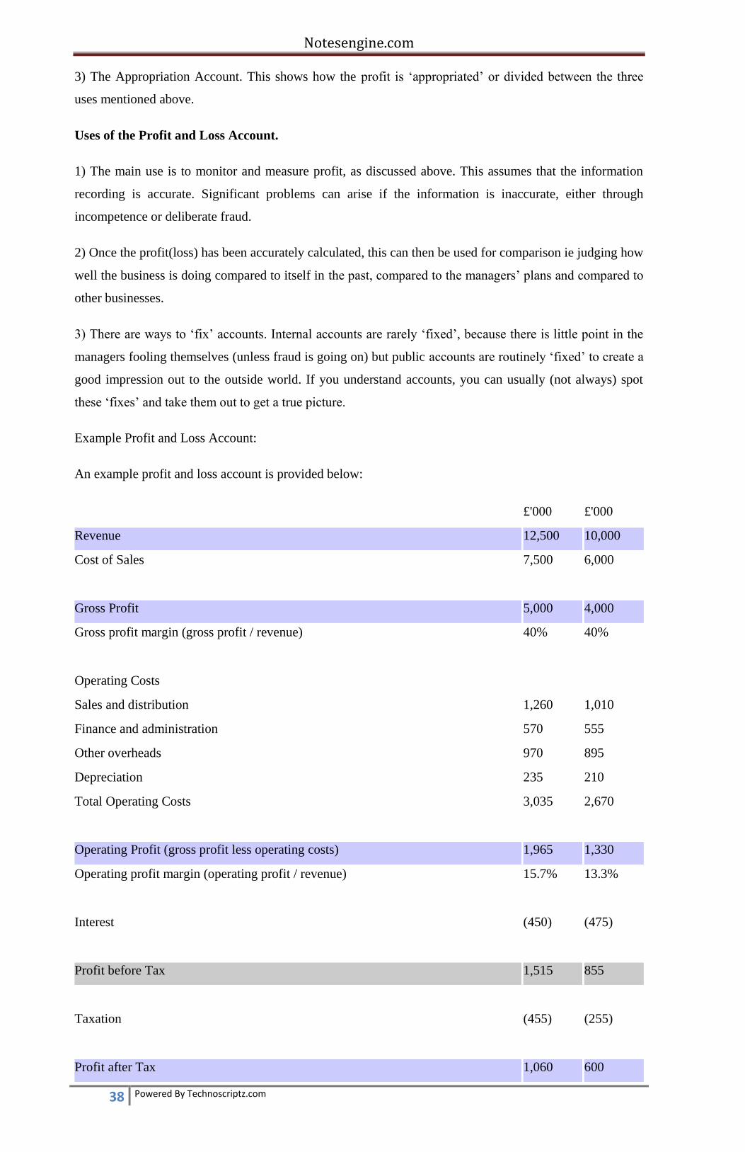
Notesengine.com
38 Powered By Technoscriptz.com
3) The Appropriation Account. This shows how the profit is ‗appropriated‘ or divided between the three
uses mentioned above.
Uses of the Profit and Loss Account.
1) The main use is to monitor and measure profit, as discussed above. This assumes that the information
recording is accurate. Significant problems can arise if the information is inaccurate, either through
incompetence or deliberate fraud.
2) Once the profit(loss) has been accurately calculated, this can then be used for comparison ie judging how
well the business is doing compared to itself in the past, compared to the managers‘ plans and compared to
other businesses.
3) There are ways to ‗fix‘ accounts. Internal accounts are rarely ‗fixed‘, because there is little point in the
managers fooling themselves (unless fraud is going on) but public accounts are routinely ‗fixed‘ to create a
good impression out to the outside world. If you understand accounts, you can usually (not always) spot
these ‗fixes‘ and take them out to get a true picture.
Example Profit and Loss Account:
An example profit and loss account is provided below:
£'000 £'000
Revenue 12,500 10,000
Cost of Sales 7,500 6,000
Gross Profit 5,000 4,000
Gross profit margin (gross profit / revenue) 40% 40%
Operating Costs
Sales and distribution 1,260 1,010
Finance and administration 570 555
Other overheads 970 895
Depreciation 235 210
Total Operating Costs 3,035 2,670
Operating Profit (gross profit less operating costs) 1,965 1,330
Operating profit margin (operating profit / revenue) 15.7% 13.3%
Interest (450) (475)
Profit before Tax 1,515 855
Taxation (455) (255)
Profit after Tax 1,060 600

Notesengine.com
39 Powered By Technoscriptz.com
Dividends 650 400
Retained Profits 410 200
In this series of articles we will also discuss:
1. Balance Sheet Explained
2. Trading and Profit and Loss Account
3. Adjustments of Final Accounts
Previously while discussing the basic accounting equation it was noted that A - L = P, where A represents
assets (property and possession) owned by the business; L represents liabilities (claims against the business
of the creditors) and P represents the proprietor's funds (equity) in the business.,
Accounting Concept of Income
The concept of 'income' is different to the economists and accountants. Economists concept of income is
that of 'real income' meaning thereby the increase-in real terms of the ownership funds between two points
of time.
In accounting the term income is known as 'net profit'. It was stated earlier :
Sales - Merchandising cost = Gross profit and Gross profit - Expenses of doing business = Net profit
In other words, Revenue - Expenses = Net profit.
These terms are explained below:
Revenue
It is the monetary value of the products sold or services rendered to the customers during the period. It
results from sales services and source like interest, dividend and commission etc. For example, sales
affected by the business and charge made for services rendered by the business constitutes revenue.
However, all cash receipt may nott be revenue.
Thus, money borrowed leads to cash receipt but it does not constitute revenue. Similarly additional capital
brought in increases proprietor's funds but it is not revenue.
Expenses/Cost of (doing business)
Expenditure incurred by the business to earn revenue is termed as expense or cost of doing business.
Examples of expenses are raw materials consumed, salaries, rent, depreciation, advertisement etc.
Cash v/s Accrual Basis of Accounting
Small business, individual professionals and non-trading concerns usually adopt cash basis of accounting.
Under this system, incomes are considered to have been earned only when received ill cash and expenses
are considered to have been incurred only actually paid. Hence, under this system the profit or loss of an
Notesengine.com
40 Powered By Technoscriptz.com
accounting period is the difference between incomes received and the expenses paid. Though the cash basis
of accounting is simple (no adjustment is required) but il loses its comparability.
Under accrual basis all incomes are credited to the period in which earned irrespective of the fact whether
received or not. Similarly, all expenses are debited to the period in which incurred irrespective of the fact
whether paid or not. It is a scientific basis of accounting, though a bit difficult.
Matching Concept. Requires that expenses should be matched to the revenues of the appropriate accounting
period. So we must determine what are the revenues earned during a particular accounting period and the
expenses incurred to earn these revenues.
It is the matching concept which justifies accrual basis of accounting.
Accruals and Deferrals
Accounting is expected to measure or ascertain the net income of the business during the accounting
period. Normally, it is the calendar year (1st January to 31st December) but in other cases it may be
Financial year (Ist April to 31st March) or any other period according to the convention of the business
community of the area.
The combined impact of matching concept and the accounting period concept on accounting has resulted in
accruals and deferrals.
Accrued or Outstanding expenses
It is the term which denotes that expenditure has been incurred during the accounting period but the same
has not been paid in cash e.g. Salary, Rent, Wage etc. becoming due but not paid.
Deferred or pre-paid expenses
It is the term which denotes that payment in cash has been made "in advance but the full benefit of this
payment has not been reaped by the current accounting period, e.g., Insurance paid in advance.
Accrued or outstanding Income
It is the term which denotes that the income has been earned but the cash has not been received against the
same. Income has accrued due but not received e.g. Interest on investments etc.
Differed or Received in-advance Income
It is the term which denotes income which has been received (in cash) in advance but it has not been earned
so far e.g. rent received in advance. All the accruals and deferrals arc not be adjusted at the end of the
accounting period (end-period adjustments) in order to find out the income of the business during the
period under review. The procedure of ascertaining (i) business income and (ii) financial position is being
described, in detail below:
In fact, these arc two most important of many objectives of book-keeping. In order to know the profits
earned by him he prepares a trading and loss account and in order to know the financial position of his
business on the last day of the financial period he prepares a balance sheet.
Such accounts are called 'Final Accounts'. Preparation of final accounts is the concluding step of
accounting cycle. In fact, final accounts include a number of accounts (i) Manufacturing/ Production
account, (ii) Trading account, (iii) Profit and loss account and (iv) Balance sheet.
Notesengine.com
41 Powered By Technoscriptz.com
Practically balance sheet is a statement but for accounting purposes here it is treated as a part vital
accounts.
The preparation of above all or any of the above accounts depends upon the nature of the business being
carried on by the business concerned. In case of a manufacturing business manufacturing account, trading
account, profit and loss account and balance sheet form the parts of final accounts whereas in case of
trading business all other accounts are prepared with the exception of manufacturing account. Each of these
accounts provide a specific vital information to businessman to help to control and organize the business
activities in a batter way.
Cash Flow Statement
Complementing the balance sheet and income statement, the cash flow statement (CFS), a mandatory part
of a company's financial reports since 1987, records the amounts of cash and cash equivalents entering and
leaving a company. The CFS allows investors to understand how a company's operations are running,
where its money is coming from, and how it is being spent. Here you will learn how the CFS is structured
and how to use it as part of your analysis of a company.
A cash fl ow statement is one of the most
important fi nancial statements for a project
or business. The statement can be as simple
as a one page analysis or may involve several
schedules that feed information into a central
statement.
A cash fl ow statement is a listing of the fl ows of cash into and out of the business or project. Think of it as
your checking account at the bank. Deposits are the cash infl ow and withdrawals (checks) are the cash
outfl ows. The balance in your checking account is your net cash fl ow at a specifi c point in time.
A cash fl ow statement is a listing of cash fl ows that occurred during the past accounting period. A
projection of future fl ows of cash is called a cash FIow budget. You can think of a cash fl ow budget as a
projection of the future deposits and withdrawals to your checking account.
A cash fl ow statement is not only concerned with the amount of the cash fl ows but also the timing of
the fl ows. Many cash fl ows are constructed with multiple time periods. For example, it may list
monthly cash infl ows and outfl ows over a year‘s time. It not only projects the cash balance remaining
at the end of the year but also the cash balance for each month.

Notesengine.com
42 Powered By Technoscriptz.com
Working capital is an important part of a cash fl ow analysis. It is defi ned as the amount of money
needed to facilitate business operations and transactions, and is calculated as current assets (cash
or near cash assets) less current liabilities (liabilities due during the upcoming accounting period).
Computing the amount of working capital gives you a quick analysis of the liquidity of the business
over the future accounting period. If working capital appears to be suffi cient, developing a cash fl ow
The Structure of the CFS
The cash flow statement is distinct from the income statement and balance sheet because it does not include
the amount of future incoming and outgoing cash that has been recorded on credit. Therefore, cash is not
the same as net income, which, on the income statement and balance sheet, includes cash sales and sales
made on credit. (To learn more about the credit crisis, read Liquidity And Toxicity: Will TARP Fix The
Financial System?)
Cash flow is determined by looking at three components by which cash enters and leaves a company: core
operations, investing and financing,
Operations
Measuring the cash inflows and outflows caused by core business operations, the operations component of
cash flow reflects how much cash is generated from a company's products or services. Generally, changes
made in cash, accounts receivable, depreciation, inventory and accounts payable are reflected in cash from
operations.
Cash flow is calculated by making certain adjustments to net income by adding or subtracting differences
in revenue, expenses and credit transactions (appearing on the balance sheet and income statement)
resulting from transactions that occur from one period to the next. These adjustments are made because
non-cash items are calculated into net income (income statement) and total assets and liabilities (balance
sheet). So, because not all transactions involve actual cash items, many items have to be re-evaluated when
calculating cash flow from operations.
For example, depreciation is not really a cash expense; it is an amount that is deducted from the total value
of an asset that has previously been accounted for. That is why it is added back into net sales for calculating
cash flow. The only time income from an asset is accounted for in CFS calculations is when the asset is
sold.
Changes in accounts receivable on the balance sheet from one accounting period to the next must also be
reflected in cash flow. If accounts receivable decreases, this implies that more cash has entered the
company from customers paying off their credit accounts - the amount by which AR has decreased is then
added to net sales. If accounts receivable increase from one accounting period to the next, the amount of
the increase must be deducted from net sales because, although the amounts represented in AR are revenue,
they are not cash.
An increase in inventory, on the other hand, signals that a company has spent more money to purchase

Notesengine.com
43 Powered By Technoscriptz.com
more raw materials. If the inventory was paid with cash, the increase in the value of inventory is deducted
from net sales. A decrease in inventory would be added to net sales. If inventory was purchased on credit,
an increase in accounts payable would occur on the balance sheet, and the amount of the increase from one
year to the other would be added to net sales.
The same logic holds true for taxes payable, salaries payable and prepaid insurance. If something has been
paid off, then the difference in the value owed from one year to the next has to be subtracted from net
income. If there is an amount that is still owed, then any differences will have to be added to net earnings.
Investing
Changes in equipment, assets or investments relate to cash from investing. Usually cash changes from
investing are a "cash out" item, because cash is used to buy new equipment, buildings or short-term assets
such as marketable securities. However, when a company divests of an asset, the transaction is considered
"cash in" for calculating cash from investing.
Financing
Changes in debt, loans or dividends are accounted for in cash from financing. Changes in cash from
financing are "cash in" when capital is raised, and they're "cash out" when dividends are paid. Thus, if a
company issues a bond to the public, the company receives cash financing; however, when interest is paid
to bondholders, the company is reducing its cash.
Analyzing an Example of a CFS
Let's take a look at this CFS sample:
From this CFS, we can see that the cash flow for FY 2003 was $1,522,000. The bulk of the positive cash
flow stems from cash earned from operations, which is a good sign for investors. It means that core
operations are generating business and that there is enough money to buy new inventory. The purchasing of
new equipment shows that the company has cash to invest in inventory for growth. Finally, the amount of
cash available to the company should ease investors' minds regarding the notes payable, as cash is plentiful
to cover that future loan expense.
Of course, not all cash flow statements look this healthy, or exhibit a positive cash flow. But a negative
Notesengine.com
44 Powered By Technoscriptz.com
cash flow should not automatically raise a red flag without some further analysis. Sometimes, a negative
cash flow is a result of a company's decision to expand its business at a certain point in time, which would
be a good thing for the future. This is why analyzing changes in cash flow from one period to the next gives
the investor a better idea of how the company is performing, and whether or not a company may be on the
brink of bankruptcy or success.
Tying the CFS with the Balance Sheet and Income Statement
As we have already discussed, the cash flow statement is derived from the income statement and the
balance sheet. Net earnings from the income statement is the figure from which the information on the CFS
is deduced. As for the balance sheet, the net cash flow in the CFS from one year to the next should equal
the increase or decrease of cash between the two consecutive balance sheets that apply to the period that the
cash flow statement covers. (For example, if you are calculating a cash flow for the year 2000, the balance
sheets from the years 1999 and 2000 should be used.)
Conclusion
A company can use a cash flow statement to predict future cash flow, which helps with matters in
budgeting. For investors, the cash flow reflects a company's financial health: basically, the more cash
available for business operations, the better. However, this is not a hard and fast rule. Sometimes a negative
cash flow results from a company's growth strategy in the form of expanding its operations.
By adjusting earnings, revenues, assets and liabilities, the investor can get a very clear picture of what some
people consider the most important aspect of a company: how much cash it generates and, particularly, how
much of that cash stems from core operations.
FINANCIAL STATEMENT ANALYSIS
MEANING
‖Tearing apart‖ the financial statements
and looking at the relationships
Who analyzes financial statements?
Internal users (i.e., management)
External users (emphasis of chapter)
Examples?
Investors, creditors, regulatory agencies & …
stock market analysts and
auditors
What do internal users use it for?
Planning, evaluating and controlling company operations
What do external users use it for?
Assessing past performance and current financial position and making predictions about the future
profitability and solvency of the company as well as evaluating the effectiveness of management
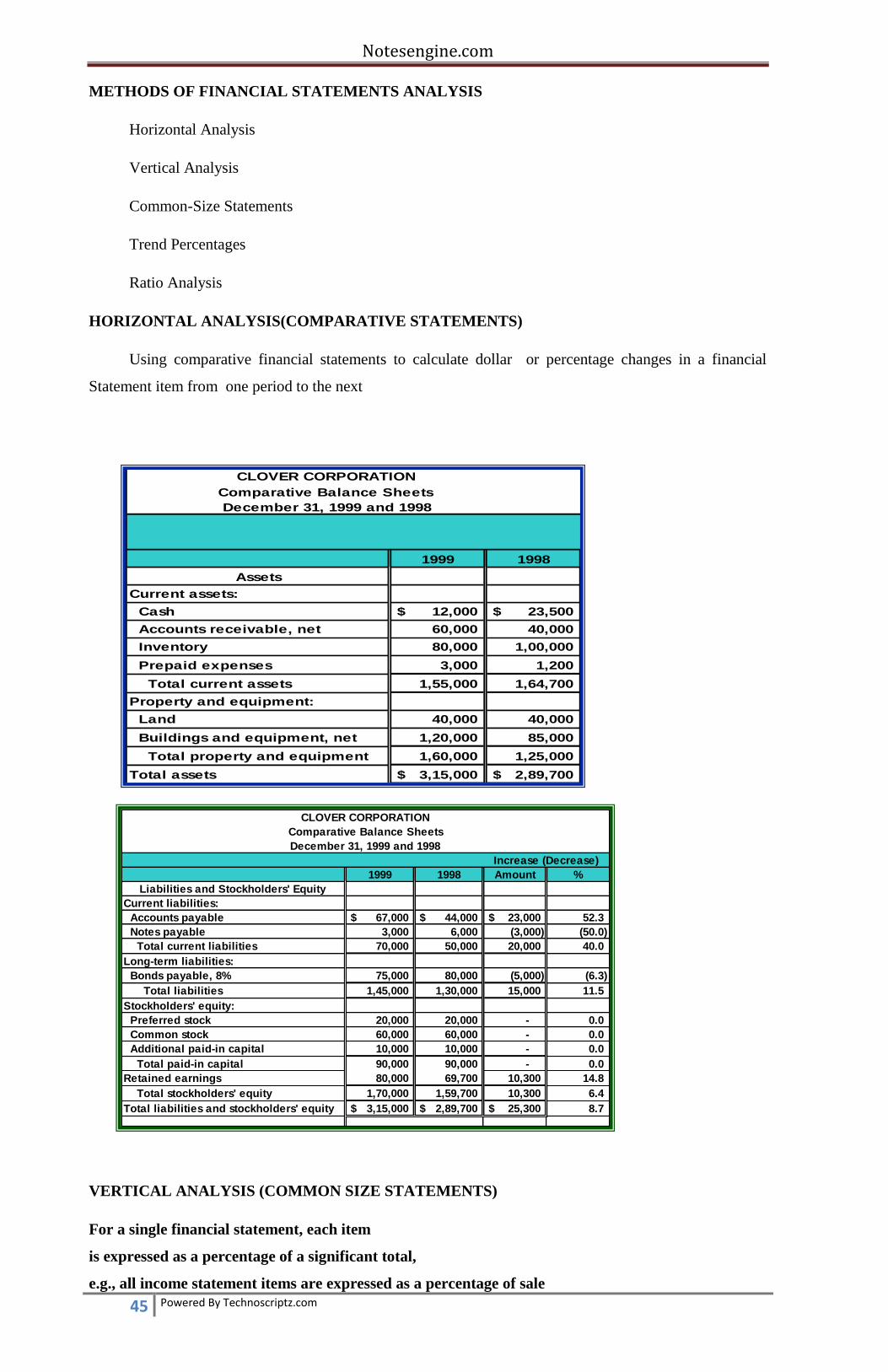
Notesengine.com
45 Powered By Technoscriptz.com
METHODS OF FINANCIAL STATEMENTS ANALYSIS
Horizontal Analysis
Vertical Analysis
Common-Size Statements
Trend Percentages
Ratio Analysis
HORIZONTAL ANALYSIS(COMPARATIVE STATEMENTS)
Using comparative financial statements to calculate dollar or percentage changes in a financial
Statement item from one period to the next
VERTICAL ANALYSIS (COMMON SIZE STATEMENTS)
For a single financial statement, each item
is expressed as a percentage of a significant total,
e.g., all income statement items are expressed as a percentage of sale
CLOVER CORPORATION
Comparative Balance Sheets
December 31, 1999 and 1998
Increase (Decrease)
1999 1998 Amount %
Assets
Current assets:
Cash 12,000$ 23,500$
Accounts receivable, net 60,000 40,000
Inventory 80,000 1,00,000
Prepaid expenses 3,000 1,200
Total current assets 1,55,000 1,64,700
Property and equipment:
Land 40,000 40,000
Buildings and equipment, net 1,20,000 85,000
Total property and equipment 1,60,000 1,25,000
Total assets 3,15,000$ 2,89,700$
CLOVER CORPORATION
Comparative Balance Sheets
December 31, 1999 and 1998
Increase (Decrease)
1999 1998 Amount %
Liabilities and Stockholders' Equity
Current liabilities:
Accounts payable 67,000$ 44,000$ 23,000$ 52.3
Notes payable 3,000 6,000 (3,000) (50.0)
Total current liabilities 70,000 50,000 20,000 40.0
Long-term liabilities:
Bonds payable, 8% 75,000 80,000 (5,000) (6.3)
Total liabilities 1,45,000 1,30,000 15,000 11.5
Stockholders' equity:
Preferred stock 20,000 20,000 - 0.0
Common stock 60,000 60,000 - 0.0
Additional paid-in capital 10,000 10,000 - 0.0
Total paid-in capital 90,000 90,000 - 0.0
Retained earnings 80,000 69,700 10,300 14.8
Total stockholders' equity 1,70,000 1,59,700 10,300 6.4
Total liabilities and stockholders' equity 3,15,000$ 2,89,700$ 25,300$ 8.7

Notesengine.com
46 Powered By Technoscriptz.com
TREND PROJECTION METHOD
Show changes over time in given financial statement items
(can help evaluate financial information of several years)
RATIO ANALYSIS
Expression of logical relationships between items in a financial statement of a single period
(e.g., percentage relationship between revenue and net income)
Liquidity Ratios
Indicate a company‘s short-term debt-paying ability
l Equity (Long-Term Solvency) Ratios
Show relationship between debt and equity financing in a company
Profitability Tests
Relate income to other variables
Market Tests
Help assess relative merits of stocks in the marketplace
CAPITAL BUDGETING
Development of a written investment policy, which is reviewed by independent
professional advisers (including legal experts as required), approved by the board,
and reviewed annually.
2. Ensuring that the written investment policy addresses the following issues
(discussed further in Section D):
■ investment committee functions and structure;
■ investment philosophy and objectives;
■ attitude to risk and process for managing risk;
■ decision rights; and
■ process for evaluating and managing investments.
3. Establishment of an investment committee if major investment is being proposed.
Key roles of the investment committee would be to:
■ establish the overall methodology, processes and controls which govern
CLOVER CORPORATION
Comparative Income Statements
For the Years Ended December 31, 1999 and 1998
Increase (Decrease)
1999 1998 Amount %
Net sales 5,20,000$ 4,80,000$ 40,000$ 8.3
Cost of goods sold 3,60,000 3,15,000 45,000 14.3
Gross margin 1,60,000 1,65,000 (5,000) (3.0)
Operating expenses 1,28,600 1,26,000 2,600 2.1
Net operating income 31,400 39,000 (7,600) (19.5)
Interest expense 6,400 7,000 (600) (8.6)
Net income before taxes 25,000 32,000 (7,000) (21.9)
Less income taxes (30%) 7,500 9,600 (2,100) (21.9)
Net income 17,500$ 22,400$ (4,900)$ (21.9)

Notesengine.com
47 Powered By Technoscriptz.com
investments;
■ ensure that robust processes (eg evaluation of fi t with the NHS foundation
trust‘s overall strategy, use of appropriate independent professional advisers)
are followed; and
■ evaluate, scrutinise and monitor investments.
4. Confirmation that the NHS foundation trust has the legal power to make the
proposed investment.
5. Engagement early on in the investment evaluation process of independent external
advisers with demonstrated expertise in advising on transactions of the size and
nature being proposed.
6. Rigorous evaluation of all proposed major investments using a thorough evaluation,
execution, and monitoring process, such as the one described in Appendix 1.
Risk Evaluation for Investment
Decisions by NHS Foundation Trusts
D. Key elements of investment policy
A best practice investment policy will contain the following elements:
(i) Investment committee functions and structure
Typically the functions of the investment committee will be to approve investment and
borrowing strategy and policies, approve performance benchmarks, review performance
against the benchmarks, ensure proper safeguards are in place for security of the NHS
foundation trust‘s funds, monitor compliance with treasury policies and procedures,
approve proposals for acquisition and disposal of assets above a de minimis amount
and approve external funding arrangements within their delegated authority.
The investment committee will comprise executive and non-executive directors, with a
majority of non-executive directors. It should be chaired by a non-executive director with
relevant investment decision-making experience. It may be a committee of the board,
or the board itself in the case of smaller NHS foundation trusts.
(ii) Investment philosophy and objectives
A best practice statement of investment philosophy and objectives will provide the
criteria for selecting the NHS foundation trust‘s investments, and address the following:
1. the statutory and principal purpose of the NHS foundation trust – the provision
of goods and services for the health service in England;
2. the NHS foundation trust‘s corporate strategy (including geographic and
service focus);
3. target rates of return for investments and explanation of how rates of return
will be calculated (eg return net of any cross-subsidies); and
4. time frame for realising the desired return on investments.
06 – 07
(iii) Attitude to risk and process for managing risk
Risk refers to the probability of an adverse outcome that is different from the expected
outcome and the potential impact of such an outcome. Some major categories of
investment risk include:
1. Strategic: risks associated with a particular strategy, for instance, overcapacity,
product or service line obsolescence, competitor reactions;
2. Financial: risks associated with the fi nancial structure of a business, the fi nancial

Notesengine.com
48 Powered By Technoscriptz.com
transactions made by the business, and the fi nancial systems which are in place,
for instance, interest rate risk, foreign exchange risk and credit risk;
3. Operational: risks associated with the operational and administrative procedures
of a business, such as, clinical operations, supply chain management, IT systems,
recruitment, labour management and post-merger integration process;
4. Regulatory and political: risks posed by potential changes in the regulatory
and political environment, such as, tariff changes, policy changes and changes
in healthcare targets;
5. Reputational: risks to the perceived quality or brand of an institution, for instance,
through bad press resulting from association with a failed joint venture;
6. Contingent: risks that will only come into existence if a certain contingent
event takes place, for instance, guarantees of a joint venture that are only
payable if it defaults.
Risk management refers to the collective set of processes, working practices and
tools used to minimise the probability and impact of adverse outcomes. It entails:
■ identifying potential sources of risk;
■ estimating value at risk, calculated as probability of loss x severity of loss;
■ implementing controls to minimise probability and severity of loss.
It is best practice to defi ne in the investment policy the NHS foundation trust‘s principles
for managing risk aligned with its corporate strategy. Examples of risk management
principles include:
■ guidelines on identifi cation of different types of risk;
■ methodology for calculating value at risk;
■ expected returns of individual investments for a given risk level – higher risk
investments require higher expected returns;
■ aggregate targeted rate of return across the portfolio of investments;
■ limitations on the locations and types of investments that can be pursued. For instance,
the policy may specify that investments in overseas ventures should only be within
the ‗core competence‘ of the organisation and within stated risk concentrations for
each geography;
■ guidelines for asset diversifi cation outside core operations. For instance, specifying
that either the organisation will not diversify outside the health sector in England,
or specifying limits on concentration of risk in a particular technology or sector.
A best practice investment policy will provide the criteria for categorising investments
by level of risk (eg high, medium and low risk). Criteria for assessing riskiness of an
investment include:
■ fi nancial magnitude of deal;
■ probability of loss;
■ complexity of the deal structure;
■ distance from an NHS foundation trust‘s core capabilities and operations;
■ fi nancing arrangements, for instance, type of debt fi nance;
■ geographic location, for instance, investment in a highly competitive, uncertain,
or unfamiliar territory will increase risk;
■ degree of operating risk assumed, be it construction risk or cost overrun risk,
for example;
Notesengine.com
49 Powered By Technoscriptz.com
■ level of post-investment management required (eg post acquisition integration).
Best practice is to scrutinise investments in proportion to risk. For example, an
NHS foundation trust board may accept ‗routine scrutiny‘ for low-risk investments
(eg decisions delegated to the investment committee, with a short-form business
case), but require ‗special scrutiny‘ for high-risk investments (eg engagement of
external independent advisers for in-depth business case, and main board approval).
While it is for NHS foundation trusts to determine their own thresholds for each
level of risk and associated scrutiny, the approach used by Monitor for its own risk
assessment may provide a useful reference point (see Section E).
It is best practice for NHS foundation trusts to seek advice from appropriate
independent external advisers (eg risk management consultants) when developing
their approach to managing risk.
Risk Evaluation for Investment
Decisions by NHS Foundation Trusts
(iv) Decision rights
A best practice investment policy will defi ne clearly the roles, responsibilities and
approval limits of the various committees and individuals with investment oversight.
These are likely to include the board, investment committee, fi nance director, and
business development group, if one exists. For example, the board might be required
to approve the written investment policy and all ‗high risk‘ investments, while the
investment committee might approve all other investments and ensure that investment
decisions follow the guidelines laid out in the written investment policy.
(v) Process for evaluating and managing investments
A robust investment policy will explain the internal processes for evaluating, executing,
and performance managing investments. The extent of review/due diligence needs to
be appropriate to the investment proposed. For example, all major investments would
be expected to undergo detailed business case evaluation and challenge.
An example of a robust framework for evaluating and managing investments is set out
in Appendix 1. This framework describes the key phases in making a major investment
decision: preliminary review, detailed review, and execution and monitoring. For each
of these phases it provides a list of key questions that board members will ask and
also lists the types of external advisers that will likely be engaged.
This risk evaluation framework is an indication of the type of analysis required at each
of the three stages of investment appraisal. If an NHS foundation trust is unclear about
how to apply the framework to a particular investment appraisal they should seek
professional advice.
08 – 09
Each potential project's value should be estimated using a discounted cash flow (DCF) valuation, to find its
net present value (NPV). (First applied to Corporate Finance by Joel Dean in 1951; see also Fisher
separation theorem, John Burr Williams: Theory.) This valuation requires estimating the size and timing of
all of the incremental cash flows from the project. These future cash flows are then
discount [disambiguation needed]ed to determine their present value. These present values are then
summed, to get the NPV. See also Time value of money. The NPV decision rule is to accept all positive
Notesengine.com
50 Powered By Technoscriptz.com
NPV projects in an unconstrained environment, or if projects are mutually exclusive, accept the one with
the highest NPV(GE)
The NPV is greatly affected by the discount rate, so selecting the proper rate - sometimes called the hurdle
rate - is critical to making the right decision. The hurdle rate is the minimum acceptable return on an
investment. It should reflect the riskiness of the investment, typically measured by the volatility of cash
flows, and must take into account the financing mix. Managers may use models such as the CAPM or the
APT to estimate a discount rate appropriate for each particular project, and use the weighted average cost
of capital (WACC) to reflect the financing mix selected. A common practice in choosing a discount rate for
a project is to apply a WACC that applies to the entire firm, but a higher discount rate may be more
appropriate when a project's risk is higher than the risk of the firm as a whole.
Internal rate of return
The internal rate of return (IRR) is defined as the discount rate that gives a net present value (NPV) of zero.
It is a commonly used measure of investment efficiency.
The IRR method will result in the same decision as the NPV method for (non-mutually exclusive) projects
in an unconstrained environment, in the usual cases where a negative cash flow occurs at the start of the
project, followed by all positive cash flows. In most realistic cases, all independent projects that have an
IRR higher than the hurdle rate should be accepted. Nevertheless, for mutually exclusive projects, the
decision rule of taking the project with the highest IRR - which is often used - may select a project with a
lower NPV.
In some cases, several zero NPV discount rates may exist, so there is no unique IRR. The IRR exists and is
unique if one or more years of net investment (negative cash flow) are followed by years of net revenues.
But if the signs of the cash flows change more than once, there may be several IRRs. The IRR equation
generally cannot be solved analytically but only via iterations.
One shortcoming of the IRR method is that it is commonly misunderstood to convey the actual annual
profitability of an investment. However, this is not the case because intermediate cash flows are almost
never reinvested at the project's IRR; and, therefore, the actual rate of return is almost certainly going to be
lower. Accordingly, a measure called Modified Internal Rate of Return (MIRR) is often used.
Despite a strong academic preference for NPV, surveys indicate that executives prefer IRR over
NPV[citation needed], although they should be used in concert. In a budget-constrained environment,
efficiency measures should be used to maximize the overall NPV of the firm. Some managers find it
intuitively more appealing to evaluate investments in terms of percentage rates of return than dollars of
NPV.
Capital budgeting (or investment appraisal) is the planning process used to determine whether a firm's long
term investments such as new machinery, replacement machinery, new plants, new products, and research
development projects are worth pursuing. It is budget for major capital, or investment, expenditures.[1]
Many formal methods are used in capital budgeting, including the techniques such as
Accounting rate of return
Net present value

Notesengine.com
51 Powered By Technoscriptz.com
Internal rate of return
Modified internal rate of return
These methods use the incremental cash flows from each potential investment, or project Techniques based
on accounting earnings and accounting rules are sometimes used - though economists consider this to be
improper - such as the accounting rate of return, and "return on investment." Simplified and hybrid methods
are used as well, such as payback period and discounted payback period.
Each potential project's value should be estimated using a discounted cash flow (DCF) valuation, to find its
net present value (NPV). (First applied to Corporate Finance by Joel Dean in 1951; see also Fisher
separation theorem, John Burr Williams: Theory.) This valuation requires estimating the size and timing of
all of the incremental cash flows from the project. These future cash flows are then
discount [disambiguation needed]ed to determine their present value. These present values are then
summed, to get the NPV. See also Time value of money. The NPV decision rule is to accept all positive
NPV projects in an unconstrained environment, or if projects are mutually exclusive, accept the one with
the highest NPV(GE)
NET PRESENT VALUE
The NPV is greatly affected by the discount rate, so selecting the proper rate - sometimes called the hurdle
rate - is critical to making the right decision. The hurdle rate is the minimum acceptable return on an
investment. It should reflect the riskiness of the investment, typically measured by the volatility of cash
flows, and must take into account the financing mix. Managers may use models such as the CAPM or the
APT to estimate a discount rate appropriate for each particular project, and use the weighted average cost
of capital (WACC) to reflect the financing mix selected. A common practice in choosing a discount rate for
a project is to apply a WACC that applies to the entire firm, but a higher discount rate may be more
appropriate when a project's risk is higher than the risk of the firm as a whole.
Internal rate of return
Main article: Internal rate of return
The internal rate of return (IRR) is defined as the discount rate that gives a net present value (NPV) of zero.
It is a commonly used measure of investment efficiency.
The IRR method will result in the same decision as the NPV method for (non-mutually exclusive) projects
in an unconstrained environment, in the usual cases where a negative cash flow occurs at the start of the
project, followed by all positive cash flows. In most realistic cases, all independent projects that have an
IRR higher than the hurdle rate should be accepted. Nevertheless, for mutually exclusive projects, the
decision rule of taking the project with the highest IRR - which is often used - may select a project with a
lower NPV.
In some cases, several zero NPV discount rates may exist, so there is no unique IRR. The IRR exists and is
unique if one or more years of net investment (negative cash flow) are followed by years of net revenues.
But if the signs of the cash flows change more than once, there may be several IRRs. The IRR equation
generally cannot be solved analytically but only via iterations.
One shortcoming of the IRR method is that it is commonly misunderstood to convey the actual annual
profitability of an investment. However, this is not the case because intermediate cash flows are almost
Notesengine.com
52 Powered By Technoscriptz.com
never reinvested at the project's IRR; and, therefore, the actual rate of return is almost certainly going to be
lower. Accordingly, a measure called Modified Internal Rate of Return (MIRR) is often used.
Despite a strong academic preference for NPV, surveys indicate that executives prefer IRR over
NPV[citation needed], although they should be used in concert. In a budget-constrained environment,
efficiency measures should be used to maximize the overall NPV of the firm. Some managers find it
intuitively more appealing to evaluate investments in terms of percentage rates of return than dollars of
NPV.
Average rate of return
Hide links within definitionsShow links within definitions
Definition
Method of investment appraisal which determines return on investment by totaling the cash flows (over the
years for which the money was invested) and dividing that amount by the number of years.
One way of measuring an investment's profitability.To calculate,one takes the total net earnings,divides by
the total number of years the investment was held,and then divides that answer by the investment's initial
acquisition cost.
Example: Rainer spent $800,000 to buy an apartment building. After deducting all operat- ing expenses,
real estate taxes, and insurance, she receives $65,000 in the first year, $71,000 in the second year, $69,000
in the third year, and $70,000 in the fourth year. The total net earnings are $275,000. Divide that number by
the 4 years being analyzed, to reach $68,750 as an average annual return. Divide $68,750 by the initial
$800,000 investment to calculate the average rate of return of 8.59 percent.
Drawback: The procedure does not take into account the time value of money.The $65,000 received in the
first year was more valuable than the $70,000 received in the fourth year,because the $65,000 could have
been invested to earn still more money.
Payback period in capital budgeting refers to the period of time required for the return on an investment to
"repay" the sum of the original investment. For example, a $1000 investment which returned $500 per year
would have a two year payback period. The time value of money is not taken into account. Payback period
intuitively measures how long something takes to "pay for itself." All else being equal, shorter payback
periods are preferable to longer payback periods. Payback period is widely used due to its ease of use
despite recognized limitations, described below.
The term is also widely used in other types of investment areas, often with respect to energy efficiency
technologies, maintenance, upgrades, or other changes. For example, a compact fluorescent light bulb may
be described of having a payback period of a certain number of years or operating hours, assuming certain
costs. Here, the return to the investment consists of reduced operating costs. Although primarily a financial
term, the concept of a payback period is occasionally extended to other uses, such as energy payback period
(the period of time over which the energy savings of a project equal the amount of energy expended since
project inception); these other terms may not be standardized or widely used.

Notesengine.com
53 Powered By Technoscriptz.com
Payback period as a tool of analysis is often used because it is easy to apply and easy to understand for
most individuals, regardless of academic training or field of endeavour. When used carefully or to compare
similar investments, it can be quite useful. As a stand-alone tool to compare an investment with "doing
nothing," payback period has no explicit criteria for decision-making (except, perhaps, that the payback
period should be less than infinity).
The payback period is considered a method of analysis with serious limitations and qualifications for its
use, because it does not properly account for the time value of money, risk, financing or other important
considerations, such as the opportunity cost. Whilst the time value of money can be rectified by applying a
weight average cost of capital discount, it is generally agreed that this tool for investment decisions should
not be used in isolation. Alternative measures of "return" preferred by economists are net present value and
internal rate of return. An implicit assumption in the use of payback period is that returns to the investment
continue after the payback period. Payback period does not specify any required comparison to other
investments or even to not making an investment.
There is no formula to calculate the payback period, excepting the simple and non-realistic case of the
initial cash outlay and further constant cash inflows or constant growing cash inflows. To calculate the
payback period an algorithm is needed. It is easily applied in spreadsheets. The typical algorithm reduces to
the calculation of cumulative cash flow and the moment in which it turns to positive from negative.
Additional complexity arises when the cash flow changes sign several times, that is it contains outflows in
the midst or at the end of the project lifetime. The modified payback period algorithm may be applied then.
Firstly, the sum of all of the cash flows is calculated. Then the cumulative positive cash flows are
determined for each period. The modified payback period is calculated as the moment in which the
cumulative positive cash flow exceeds the total cash outflow.

Notesengine.com
54 Powered By Technoscriptz.com