NOTES ON ATTITUDE TOWARD RISK TAKING

AND THE EXPONENTIAL UTILITY FUNCTION

Craig W. Kirkwood

Department of ManagementArizona State UniversityTempe, AZ 85287-4006

September 1991Corrected April 1993

Reissued January 1997

Copyright c© 1991, Craig W. Kirkwood. All rights reserved.

ABSTRACT

This paper summarizes useful concepts for analyzing attitude toward risk takingin decision analysis practice. Particular attention is given to the exponential utilityfunction which is widely used in applications. Conditions are reviewed under whichthis utility function form is appropriate. Tables are presented which aid in using theexponential utility function, including finding the value of the risk tolerance. Theuse of the exponential utility function is considered in analyzing portfolio decisionsand determining the value of perfect information. The accuracy is considered ofan approximate formula for determining certainty equivalents when the exponentialutility function holds. Exercises on this material are also included.

NOTES ON ATTITUDE TOWARD RISK TAKING

AND THE EXPONENTIAL UTILITY FUNCTION

This paper summarizes concepts related to analyzing attitude toward risk tak-ing in decision analysis practice, with particular emphasis on the use of the exponen-tial utility function. Relevant theorems and empirical observations are presented.Informal “proofs” are presented for several theorems, but these are intended to beplausibility arguments rather than detailed proofs. Technical conditions (for exam-ple, requirements that certain functions be continuous or have continuous deriva-tives) are not presented. The reader is assumed to be familiar with basic probabilityconcepts, including probability distributions, expected values, and variances.

1. The Certainty Equivalent and the Idea Underlying Utility Functions

A difficulty with decision-making under uncertainty is illustrated by the follow-ing: You are offered an alternative with equal chances of winning $10,000 or losing$1,000. How much are you willing to pay for this? You certainly will not pay morethan $10,000, and you will certainly take the alternative if someone offers to give you$1,000 in addition to the alternative. How can you settle on a number somewherebetween these two extremes? Some thought shows that different individuals mightbe willing to pay different amounts—If you are a graduate student with just enoughmoney to make it to the end of the school year, you may have a different view ofthe risks associated with this alternative than if you are a wealthy businessman.

To develop a criterion for making decisions under uncertainty, it makes senseto start with reasonable conditions that we would wish our decision-making to obey,and then to see what criterion we must use to obey these conditions. The axioms ofconsistent choice (also sometimes called the axioms of rational choice or the axiomsof decision theory) provide such a set of conditions. These axioms and two importanttheorems that result from them are presented in Appendix A. In this section, wewill make informal plausibility arguments for the decision analysis procedures whichare implied by these axioms.

We will restrict ourselves to situations where the consequences of a decisioncan be adequately described by a single evaluation measure or evaluation attributex. For many business decisions, this will be a monetary measure, such as profit,cost, or assets, possibly discounted to account for the time value of money. We willfurther assume that preferences for x are either monotonically increasing (that is,more of x is always preferred to less) or monotonically decreasing (that is, more ofx is always less preferred). For a monetary evaluation measure, the monotonicallyincreasing case corresponds to using profit or total assets as an evaluation measure,while the monotonically decreasing case corresponds to using costs or losses as anevaluation measure.

There are situations where preferences over an evaluation measure are neithermonotonically increasing nor monotonically decreasing. For example, consider theevaluation measure “blood pressure level” to measure the results of various medicaltreatments. There is a most preferred level for this evaluation measure, and eithergreater or smaller levels are less preferred. This type of situation is not common intypical business decisions, and even in such situations it is often possible to use a

1

modified evaluation measure which is monotonic. (In the blood pressure example,the attribute “distance from the most preferred level” might be used.)

A decision maker’s attitude toward risk taking is addressed with the conceptof the certainty (or certain) equivalent, which is the certain amount that is equallypreferred to an uncertain alternative. If certainty equivalents are known for thealternatives in a decision, then it is easy to find the most preferred alternative: Itis the one with the highest (lowest) certainty equivalent if we are considering profit(cost).

The “Weak Law of Large Numbers” (Drake 1967) argues for using expectedvalues as certainty equivalents when the stakes in a decision under uncertainty aresmall. This Law shows that under general conditions the average outcome for a largenumber of independent decisions stochastically converges to the average of the ex-pected values for the selected alternatives in the decisions. (The term stochasticallyconverges means that the probability the actual value will differ from the expectedvalue by any specified amount gets closer to zero as the number of independent deci-sions increases.) Thus, if you value alternatives at more than their expected values,you will lose money over many decisions since you will only sell such alternativesfor more than they will return on average. Similarly, if you value alternatives at lessthan their expected values, you will lose money because you will sell alternatives forless than they will return on average.

However, additional factors enter when the stakes are high. Most of us wouldbe willing to pay up to the expected value of $2.50 for a lottery ticket giving us a50:50 chance of winning $10.00 or losing $5.00. On the other hand, most of us wouldnot be willing to pay as much as $25,000 for a lottery ticket with a 50:50 chanceof winning $100,000 or losing $50,000 even though $25,000 is the expected value ofthis lottery. This is because a few $50,000 losses would leave most of us withoutthe resources to continue. We cannot “play the averages” over a series of decisionswhere the stakes are this large, and thus considerations of long-run average returnsare less relevant to our decision making.

Many conservative business people are averse to taking risks. That is, theyattempt to avoid the possibility of large losses. Such individuals have certaintyequivalents that are lower than the expected values of uncertain alternatives if weare dealing with profits, or higher than the expected values if we are dealing withcosts. That is, these individuals are willing to sell the alternatives for less than thesealternatives will yield on average over many such decisions in order to avoid the riskof a loss. Intuitively, we might consider incorporating this aversion toward risk intoan analysis by replacing expected value as a decision criterion by something elsewhich weights less desirable outcomes more heavily. Thus, we might replace theexpected value of alternative A

E(x|A) =

n∑

i=1

xip(xi|A)

as a decision criterion by the expected value of some utility function u(x), that is,

E[u(x)|A] =

n∑

i=1

u(xi)p(xi|A)

2

where p(xi|A) is the probability of xi given that A is selected.

If x is total assets in hundreds of thousands of dollars, then we might haveu(x) = log(x + 1). With this utility function, higher asset positions will not receiveas much weight as with expected value and very low asset positions will receive largenegative weight. This will tend to favor alternatives that have lower risk even if theyalso have lower expected values.

The certainty equivalent CE can be determined if a utility function u(x) isknown using the relationship u(CE) = E[u(x)|A] where E[u(x)|A] is the expectationof the utility for alternative A. As an example, consider again the decision abovewhich has equal chances of either winning $100,000 or losing $50,000, and supposethat the decision maker’s initial asset position is $100,000. The expected value of thisalternative in terms of total assets is 0.5 × $200, 000 + 0.5 × $50, 000 = $125, 000.Using the logarithmic utility function shown in the preceding paragraph, we cansolve for the certainty equivalent from log(CE+1) = 0.5 log(2+1)+0.5 log(0.5+1)which gives CE = $112, 000. Thus, the alternative has a certainty equivalent whichis $13,000 less than the expected value of $125,000 when it is evaluated with theutility function. This demonstrates the aversion to taking risks that was discussedabove.

This is the basic idea underlying utility functions. Appendix A presents thetheoretical basis in more detail

2. Attitude Toward Risk Taking and Utility Function Shapes

Someone who prefers to receive the expected value of an uncertain alternativefor certain rather than the uncertain alternative is called risk averse, while someonewho finds receiving the expected value for certain to be equally preferred to thealternative is called risk neutral, and someone who prefers to receive the alternativerather than the expected value for certain is called risk seeking. The most commonattitude toward risk taking in business decision making is to be risk neutral for deci-sions with small risks and to be risk averse for decisions with larger risks. Deliberaterisk seeking behavior is sometimes seen in entrepreneurs (“I can always go back toworking for somebody else if it doesn’t work out”) or in situations where you haveto “pray for rain” because the situation is already so desperate that you are goingto be in serious trouble if you don’t have a miracle. Of course, what constitutes a“small risk” may differ depending on the size of the company. (A vice president of aFortune 500 company once commented to me, “Most of the decisions we analyze arefor a few million dollars. It is adequate to use expected value for these.” Whetherthis is true or not depends on your asset position.)

A decision maker’s attitude toward risk taking determines the shape of his orher utility function. The remainder of this paper presents various results relatingthe utility function shape to attitude toward risk taking. It is not necessary tounderstand the details of the proofs of these results in order to use utility functions,but the results themselves are important for applying decision analysis. (The proofsare indented slightly and set in smaller type.)

3

Theorem 1 (Utility Function Shapes). If risk aversion holds for all alternativeswhich have outcomes within some range over x then u(x) is concave downward overthat range of x. [That is, d2u(x)/dx2 < 0 over the range.] Similarly, risk neutralityimplies that u(x) is linear [that is d2u(x)/dx2 = 0], and risk seeking behavior impliesthat u(x) is convex downward [that is, d2u(x)/dx2 > 0.]

Proof. The result will be shown for the risk averse case, and the other cases can beproved in a similar way. The demonstration proceeds by showing that for a particulartype of uncertain alternative the utility function must be concave to yield the requiredbehavior. Since this particular type of alternative is one of the class of “all alternativeswhich have outcomes within some range of x,” this establishes the desired result.

Consider an alternative with possible outcomes x̄ − δ and x̄ + δ which are equallylikely. If the decision maker is risk averse, then this alternative must be less preferredthan receiving the expected value x̄ of the alternative. Thus, it must be true that

u(x̄) > (1/2)[u(x̄− δ) + u(x̄ + δ)].

Write the right hand side of this relation as a Taylor expansion around x̄. This leadsto

u(x̄) > (1/2)[u(x̄) − du(x̄)

dxδ + (1/2)

d2u(x̄)

dx2δ2 + · · ·

+ u(x̄) +du(x̄)

dxδ + (1/2)

d2u(x̄)

dx2δ2 + · · ·].

In the limit as δ approaches 0, this becomes

u(x̄) > u(x̄) + (1/2)d2u(x̄)

dx2δ2

which only holds if d2u(x̄)/dx2 < 0. Since x̄ can be any level of x, this establishes thedesired result.

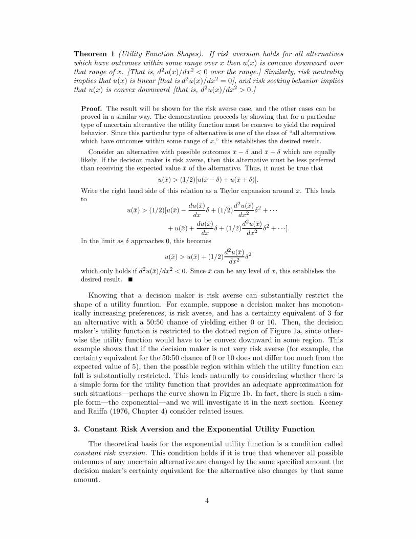
Knowing that a decision maker is risk averse can substantially restrict theshape of a utility function. For example, suppose a decision maker has monoton-ically increasing preferences, is risk averse, and has a certainty equivalent of 3 foran alternative with a 50:50 chance of yielding either 0 or 10. Then, the decisionmaker’s utility function is restricted to the dotted region of Figure 1a, since other-wise the utility function would have to be convex downward in some region. Thisexample shows that if the decision maker is not very risk averse (for example, thecertainty equivalent for the 50:50 chance of 0 or 10 does not differ too much from theexpected value of 5), then the possible region within which the utility function canfall is substantially restricted. This leads naturally to considering whether there isa simple form for the utility function that provides an adequate approximation forsuch situations—perhaps the curve shown in Figure 1b. In fact, there is such a sim-ple form—the exponential—and we will investigate it in the next section. Keeneyand Raiffa (1976, Chapter 4) consider related issues.

3. Constant Risk Aversion and the Exponential Utility Function

The theoretical basis for the exponential utility function is a condition calledconstant risk aversion. This condition holds if it is true that whenever all possibleoutcomes of any uncertain alternative are changed by the same specified amount thedecision maker’s certainty equivalent for the alternative also changes by that sameamount.

4

0 2 4 6 8 10

a. Risk Aversion

0.0

0.5

1.0UTILITY

..............................................................................................................................................................................................................................

...................................................................................................................................................................................................................................................................................

.

.

.

.

.

.

.

.

.

.

.

.

.

.

.

.

.

.

.

.

.

...........

... .. .. . .. . . .. . . . .. . . . . .. . . . . .. . . . . . .. . . . . . .. . . . . . . .. . . . . . . .. . . . . . . . .

0 2 4 6 8 10

b. Exponential Function

0.0

0.5

1.0

.....................................................................................................................

.............

.............

.............

.............

.............

.............

.............

.............

.............

.............

.............

....................................................................................................................................................................................................................................................................

...............................

...............

Figure 1. Risk Aversion and Utility Function Shapes

Theorem 2 (Constant Risk Aversion). Constant risk aversion holds if and only ifu(x) has either an exponential or linear shape. (Pratt 1964)

Proof. Showing that a linear or exponential utility function form implies that constantrisk aversion holds is straightforward. We will show that constant risk aversion impliesthat one of these forms holds, and will only consider the case where preferences aremonotonically increasing with respect to the evaluation measure. (The proof for themonotonically decreasing case is analogous.) Additional notation is useful for this proof.The risk premium for an alternative is the difference between the expected value x̄ forthe alternative and its certainty equivalent CE. Specifically, for an evaluation measurewith monotonically increasing preferences, the risk premium π is given by π = x̄−CEwhile with monotonically decreasing preferences it is π = CE − x̄. Thus, the riskpremium is positive for a risk averse decision maker, 0 for one who is risk neutral, andnegative for one who is risk seeking.

Consider two alternatives related in the manner given in the definition of constantrisk aversion. That is, the second alternative differs from the first only by having thesame amount either added to or subtracted from each outcome. It follows directlyfrom the definition of the risk premium π that the risk premiums must be the samefor the two alternatives if constant risk aversion holds. Furthermore, if z is defined byz = x − x̄, then z has the same probability distribution for both alternatives.

Suppose that the certainty equivalent of an uncertain alternative is CE. Then itmust be true that u(CE) = E[u(x)]. This can be rewritten in terms of π and z asu(x̄ − π) = E[u(x̄ + z)].

Now Taylor expand both sides of this equation around x̄. The left side becomes

u(x̄ − π) = u(x̄) − du(x̄)

dxπ + (1/2)

d2u(x̄)

dx2π2 + · · ·

and the right side becomes

E[u(x̄ + z)] = E[u(x̄) +du(x̄)

dxz + (1/2)

d2u(x̄)

dx2z2 + · · ·]

= u(x̄) +du(x̄)

dxE(z) + (1/2)

d2u(x̄)

dx2E(z2) + · · ·

Since x̄ is the expected value for the alternative and z = x − x̄, then E(z) = 0 andE(z2) = σ2 where σ2 is the variance for the alternative.

5

Using these facts, equating the right-hand and left-hand Taylor expansions, anddropping common terms leads to

−du(x̄)

dxπ + (1/2)

d2u(x̄)

dx2π2 + · · · = (1/2)

d2u(x̄)

dx2σ2 + · · ·

Now assume a situation with “small” risk aversion so that π � σ and where theuncertainty is small enough that only terms through second order need be consideredin the Taylor expansion. Then the equation above reduces to

−du(x̄)

dxπ = (1/2)

d2u(x̄)

dx2σ2

or

π = −(1/2)d2u(x̄)/dx2

du(x̄)/dxσ2 (1)

With constant risk aversion, π and σ will not change when a constant amount isadded to each possible outcome of an alternative. However, x̄ will change by theconstant amount. Thus, for Equation 1 to hold, it must be true that

d2u(x)/dx2

du(x)/dx= −c

for some constant c. (Otherwise the right hand side of Equation 1 will vary as x̄changes, and hence constant risk aversion will not hold.) This is a second-order linearconstant-coefficient differential equation, and the solution is

u(x) =

{

a + b exp(−cx), c 6= 0

a + bx, c = 0

where a and b are undetermined constants.

From Theorem A-2 in Appendix A, it follows that the values of a and b do notmatter except that b must have the correct sign so that preferences either increase ordecrease as is appropriate for the evaluation measure of interest.

The usual convention is for a utility function to be scaled so that the least pre-ferred level of the evaluation measure that is being considered has a utility of zeroand the most preferred level being considered has a utility of one. With these con-ventions, if preferences are monotonically increasing over x (that is, larger amountsof x are preferred to smaller amounts), then the exponential utility function can bewritten

u(x) =

exp [−(x − Low)/ρ]− 1

exp [−(High− Low)/ρ]− 1, ρ 6= Infinity

x − Low

High− Low, otherwise,

(2a)

and if preferences are monotonically decreasing over x, then

u(x) =

exp [−(High − x)/ρ]− 1

exp [−(High− Low)/ρ]− 1, ρ 6= Infinity

High − x

High− Low, otherwise,

(2b)

6

0 2 4 6 8 10

a. Increasing Preferences

0.0

0.5

1.0

UTILITY

ρ = 1

ρ = 5

ρ = −5ρ = −1

.............................................................................................................................................................................................................................................................................................................................................................................................................................

......

......

.....

.....

.....

.....

.....

.....

.....

.....

....

.....

....

....

....

....

....

....

....

....

.....

....

....

....

....

.....

....

.....

....................................................................................................................................................

..................................................................................

.............................................................................................................................................

...........................................................................................................................................................................................................................................................................................................................................................................

..............................

..................................

............................................................................................................................................................................................................................

.......................................................................................................................................................................................................................................................................................

..................................

..............................

..........................

.................................................................................................................................................................................................................................................................................................................................................

0 2 4 6 8 10

b. Decreasing Preferences

0.0

0.5

1.0 ρ = 1

ρ = 5

ρ = −5

ρ = −1

.............................................................................................................................................................................................................................................................................................................................................................................................................................

...................................................................................................................................................................................................................................................................................................................................................................................................................................................................................................................

...........................................................................................................................................................................................................................................................................................................................................................................................................................................

...........................................................................................................................................................................................................................................................................................................................................................................................................................................

...................................................................................................................................................................................................................................................................................................................................................................................................................................................................................................................

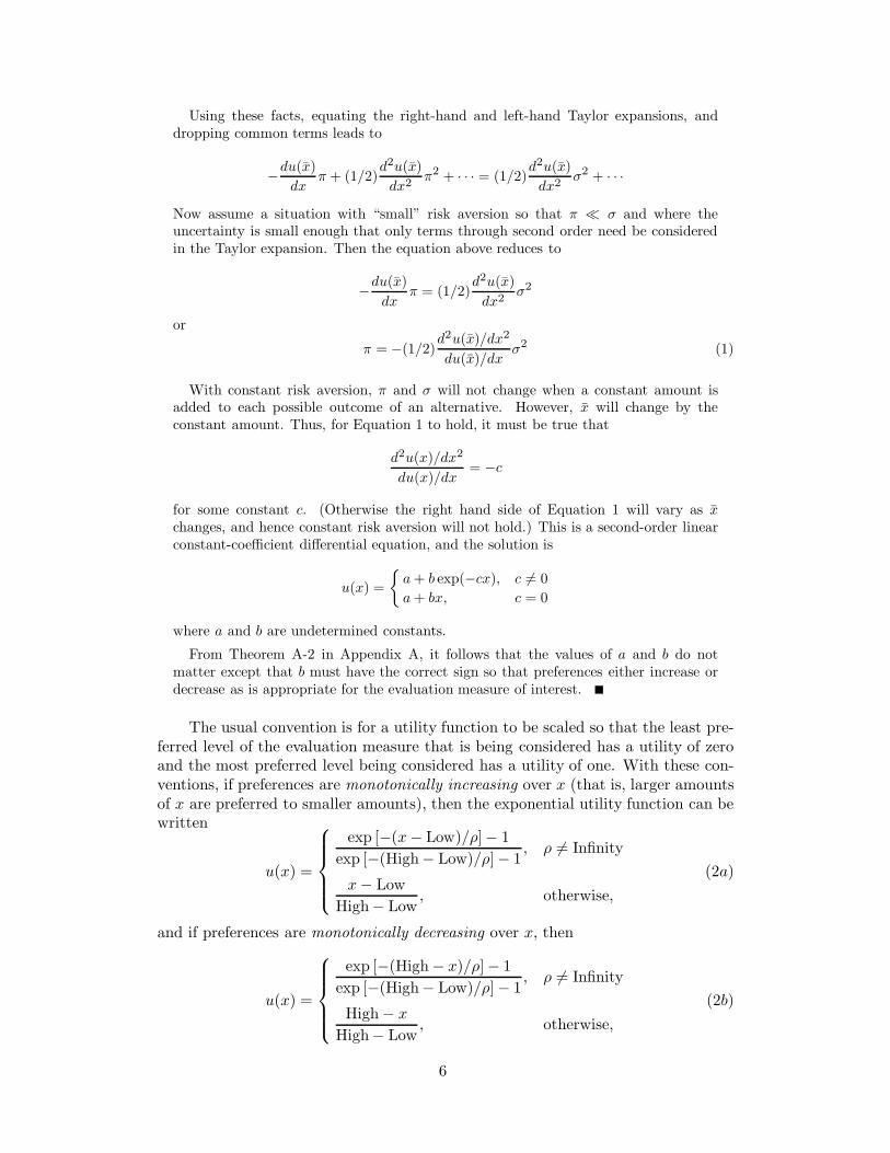
Figure 2. Exponential Utility Functions

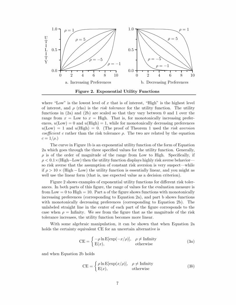
where “Low” is the lowest level of x that is of interest, “High” is the highest levelof interest, and ρ (rho) is the risk tolerance for the utility function. The utilityfunctions in (2a) and (2b) are scaled so that they vary between 0 and 1 over therange from x = Low to x = High. That is, for monotonically increasing prefer-ences, u(Low) = 0 and u(High) = 1, while for monotonically decreasing preferencesu(Low) = 1 and u(High) = 0. (The proof of Theorem 1 used the risk aversioncoefficient c rather than the risk tolerance ρ. The two are related by the equationc = 1/ρ.)

The curve in Figure 1b is an exponential utility function of the form of Equation2a which goes through the three specified values for the utility function. Generally,ρ is of the order of magnitude of the range from Low to High. Specifically, ifρ < 0.1×(High−Low) then the utility function displays highly risk averse behavior—so risk averse that the assumption of constant risk aversion is very suspect—whileif ρ > 10× (High− Low) the utility function is essentially linear, and you might aswell use the linear form (that is, use expected value as a decision criterion).

Figure 2 shows examples of exponential utility functions for different risk toler-ances. In both parts of this figure, the range of values for the evaluation measure isfrom Low = 0 to High = 10. Part a of the figure shows functions with monotonicallyincreasing preferences (corresponding to Equation 2a), and part b shows functionswith monotonically decreasing preferences (corresponding to Equation 2b). Theunlabeled straight line in the center of each part of the figure corresponds to thecase when ρ = Infinity. We see from the figure that as the magnitude of the risktolerance increases, the utility function becomes more linear.

With some algebraic manipulation, it can be shown that when Equation 2aholds the certainty equivalent CE for an uncertain alternative is

CE =

{

−ρ lnE[exp(−x/ρ)], ρ 6= InfinityE(x), otherwise

(3a)

and when Equation 2b holds

CE =

{

ρ lnE[exp(x/ρ)], ρ 6= InfinityE(x), otherwise

(3b)

7

4. Determining the Risk Tolerance

It is straightforward to show that ρ is approximately equal to the X suchthat an alternative with equal chances of winning X or losing X/2 has a certaintyequivalent of zero. It is also true that ρ is approximately equal to the X ′ such thatan alternative with a 0.75 chance of winning X ′ and a 0.25 chance of losing X ′ hasa certainty equivalent of zero.

Howard (1988) gives some rules of thumb for the size of ρ as a function ofcertain financial measures of a company. He has found values of ρ which are aboutsix percent of net sales, about 100 to 150 percent of net income, and about one-sixth of equity. (These figures were derived from companies in the oil and chemicalsindustries.) McNamee and Celona (1990) comment that a ratio of risk tolerance toequity of one-sixth or of risk tolerance to market value of one-fifth seems to translatebest across companies in different industries.

The value of ρ can be more precisely determined by eliciting the certaintyequivalent for an uncertain alternative and then solving for the ρ which gives thissame certainty equivalent. For example, consider a situation with monotonicallyincreasing preferences where the certainty equivalent for an alternative with equalchances of Low or High is CE. From Equation 2a, if CE = (Low + High)/2, thenρ = Infinity; otherwise it is the solution to

0.5 =exp[−(CE− Low)/ρ]− 1

exp[−(High− Low)/ρ]− 1(4)

This equation must be solved numerically.

Appendix B includes a table of solution values for Equation 4. To use thistable for a situation with monotonically increasing preferences, set z0.5 = (CE −Low)/(High − Low) and look this up in the table to find a corresponding value forR. Then, ρ = R×(High−Low). For monotonically decreasing preferences, the sameprocedure is followed, except that z0.5 is determined by z0.5 = (High−CE)/(High−Low). For example, suppose that preferences are monotonically decreasing, and thatthe certainty equivalent for an alternative with equal chances of $10,000 and $5,000is $8,500. Then z0.5 = ($10, 000 − $8, 500)/($10, 000 − $5, 000) = 0.3. Lookingthis entry up in the Appendix B table, we see that R = 0.56, and hence ρ =0.56× ($10, 000− $5, 000) = $2, 800.

It is straightforward to enter Equation 2 into an electronic spreadsheet or aprogrammable calculator to determine values for u(x) once ρ is known. The tablein Appendix C can also be used to find u(x). (A Pascal computer program to solveEquation 4 is given in Appendix D.)

5. Portfolios of Independent Alternatives

Suppose that you have a portfolio of n different alternatives where the totaloutcome s from all the alternatives is the sum of the outcomes x1, x2, . . . , xn fromthe different alternatives. When constant risk aversion holds and the alternativesare probabilistically independent, the certainty equivalent CE for the portfolio is thesum of the certainty equivalents CE1, CE2, . . . , CEn for the individual alternatives.

8

Proof. Assume that the exponential case of Equation 2a holds. (The proofs forthe other cases are analogous.) Then from Equation 3a, CE = −ρ ln E[exp(−s/ρ)] =−ρ ln E{exp[−(

∑ni=1

xi)/ρ]} = −ρ ln E[∏n

i=1exp(−xi/ρ)]. Since the xi are proba-

bilistically independent, this reduces to CE =∑n

i=1 −ρ lnE[exp(−xi/ρ)]. By similarreasoning, CEi = −ρ lnE[exp(−xi/ρ)]. Comparing these two equations, we see thatCE =

∑ni=1

CEi.

6. The Value of Perfect Information

A straightforward argument shows that when constant risk aversion holds thevalue of perfect information is the difference between the certainty equivalent of theperfect information alternative ignoring the cost of the information and the cer-tainty equivalent of the best alternative without perfect information. The followingargument demonstrates that this is true: The perfect information alternative takinginto account the cost of the information differs from the perfect information alter-native ignoring the cost of the information only by having a constant amount (thecost of the information) subtracted from each possible outcome. Thus, from thedefinition of constant risk aversion, the certainty equivalent for the perfect infor-mation alternative including the cost of information must be equal to the certaintyequivalent of the perfect information alternative ignoring the cost of the informationminus the cost of the information. Hence, the value of perfect information can bedetermined by taking the difference between the certainty equivalents of the perfectinformation alternative ignoring the cost of the information and the best alternativewithout perfect information.

Note that this is not true for all utility functions. Most introductory decisionanalysis textbooks restrict themselves to treating the value of information only whenexpected value is used as a decision criterion. Since this is a special case of constantrisk aversion, the value of perfect information can be determined as specified in thepreceding paragraph. However, it is easy to construct counterexamples which showthat this procedure does not give the correct answer for utility functions that areneither exponential nor linear.

7. Approximations Using Exponential Utility Functions

From Equation 1, it follows that when constant risk aversion holds the certaintyequivalent CE for an alternative with monotonically increasing preferences is givenapproximately by

CE = x̄ − σ2

2ρ(5)

where x̄ is the expected value of the alternative, and σ2 is the variance of thealternative. (With monotonically decreasing preferences, the equation is the sameexcept that the minus sign is changed to a plus sign.) It is possible to show by directcalculation that Equation 5 is exact for an exponential utility function when analternative has a Normal (Gaussian) probability distribution for its outcomes. Thissection presents the results of some empirical studies which show that Equation 5 canbe a fairly accurate approximation even when the alternative has a distribution thatis not very Normal. However, before presenting these results, note that in situations

9

where Equation 5 is valid, it can be used to make some statements about the typesof decisions where considering risk aversion can change the preferred decision.

Howard [1988] notes,

While the ability to capture risk preference is an important part of our conceptualview of decision-making, I find it is a matter of real practical concern in only 5percent to 10 percent of business decision analysis. Of course, the situations thatrequire risk preference, such as bidding or portfolio problems, use it very seriously.

Equation 5 gives a basis for this observation. Using this equation, the differencebetween the expected value and the certainty equivalent is σ2/(2ρ). Hence, theranking of alternatives will be impacted by risk attitude (which is encoded by ρ)only if σ2 differs among the alternatives. That is, the amount of uncertainty (asmeasured by σ2) must differ among the alternatives for risk attitude to impact theranking of alternatives. Otherwise, the term σ2/(2ρ) merely adds the same constantcorrection to the expected value for each alternative, and hence expected value willcorrectly rank alternatives even though it will give incorrect certainty equivalents.

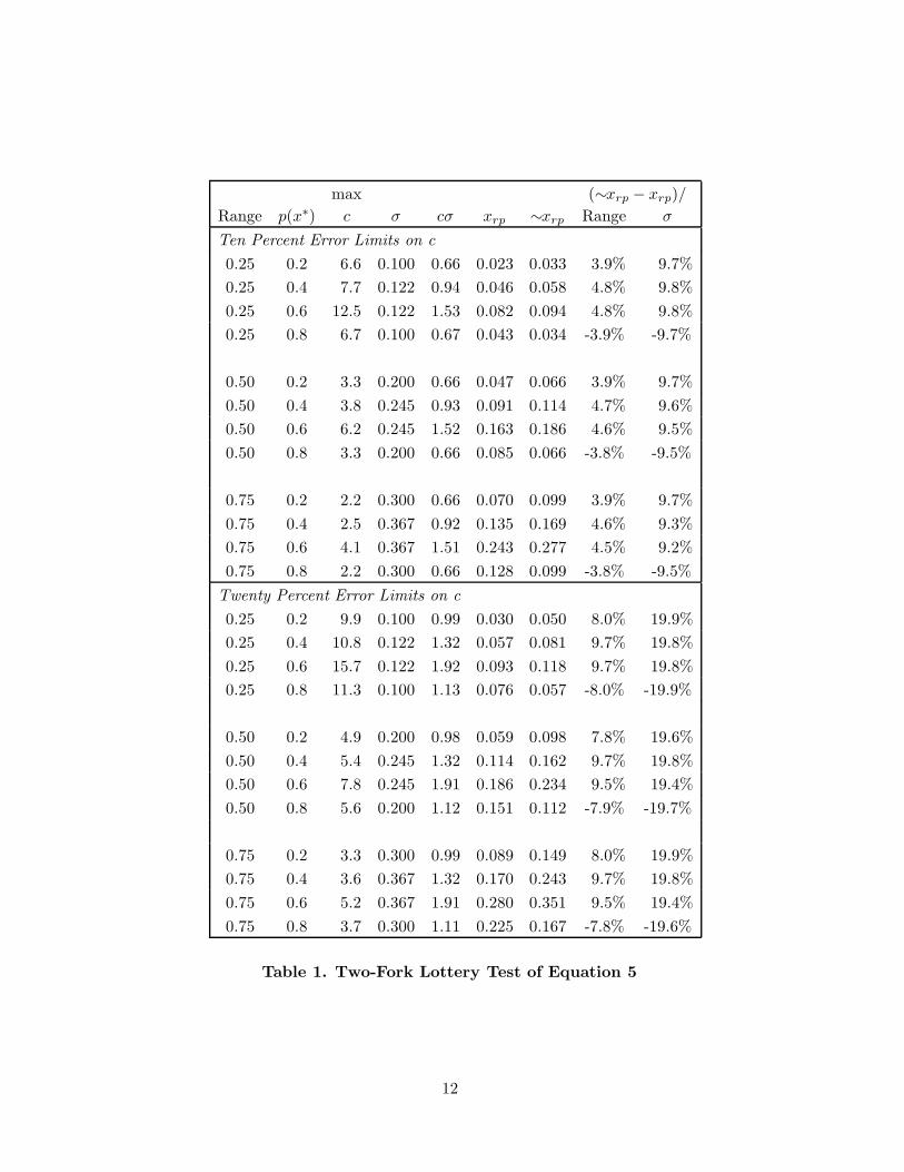
The accuracy of Equation 5 is investigated below for two families of probabil-ity distributions over x: asymmetric two-fork lotteries (that is, distributions withtwo possible outcomes and unequal probabilities for the two outcomes) and betadistributions. These two distribution families were studied because they provideconsiderable flexibility regarding specific distribution shapes and because togetherthey cover situations that are representative of those seen in practice. The resultsof the accuracy studies are shown in Table 1 for the asymmetric two-fork lottery,and in Table 2 for the beta distribution.

To study the accuracy of the approximations, it is first necessary to establishscales for measuring errors. For the two fork lottery, two measures are used: theerror as a percentage of the range between the upper and lower fork values andthe error as a percentage of the standard deviation of the lottery. (The standarddeviation is used for comparison because it is a commonly used summary of theuncertainty represented by a probability distribution.)

In Table 1, “Range” is the difference between the values of x for the higher andlower forks of the lottery, p(x∗) is the probability of the higher value, c is the riskaversion coefficient, σ is the standard deviation of x for the two fork lottery, cσ is theproduct of c and the standard deviation (from the Taylor expansion development inTheorem 2, Equation 5 will certainly be an accurate approximation when cσ � 1),xrp is the exact risk premium for the two-fork lottery using Equation 2a, ∼xrp is theapproximate risk premium calculated using Equation 5, and the last two columnsgive the differences between the approximate and exact risk premiums as a percentof the range and standard deviation of the lottery respectively. These two ratiossummarize the accuracy of the approximation relative to the uncertainty in the twofork lottery. (For smaller values of the ratios, the approximation is more accurate.)

The upper half of Table 1 gives the maximum values of c for which the errorusing Equation 5 is less than ten percent of the standard deviation of x for variouscombinations of Range and p(x∗), and the lower half of the table gives the maximumvalues of c for which the error is less than twenty percent of the standard deviation.(These maximum values are given in the column labeled “max c.”) This tableshows that for cσ approaching or even exceeding 1 Equation 5 is still a reasonablyaccurate approximation; the values of c for which Equation 5 is accurate cover

10

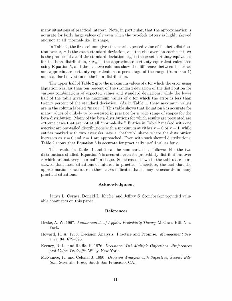
many situations of practical interest. Note, in particular, that the approximation isaccurate for fairly large values of c even when the two-fork lottery is highly skewedand not at all “normal-like” in shape.

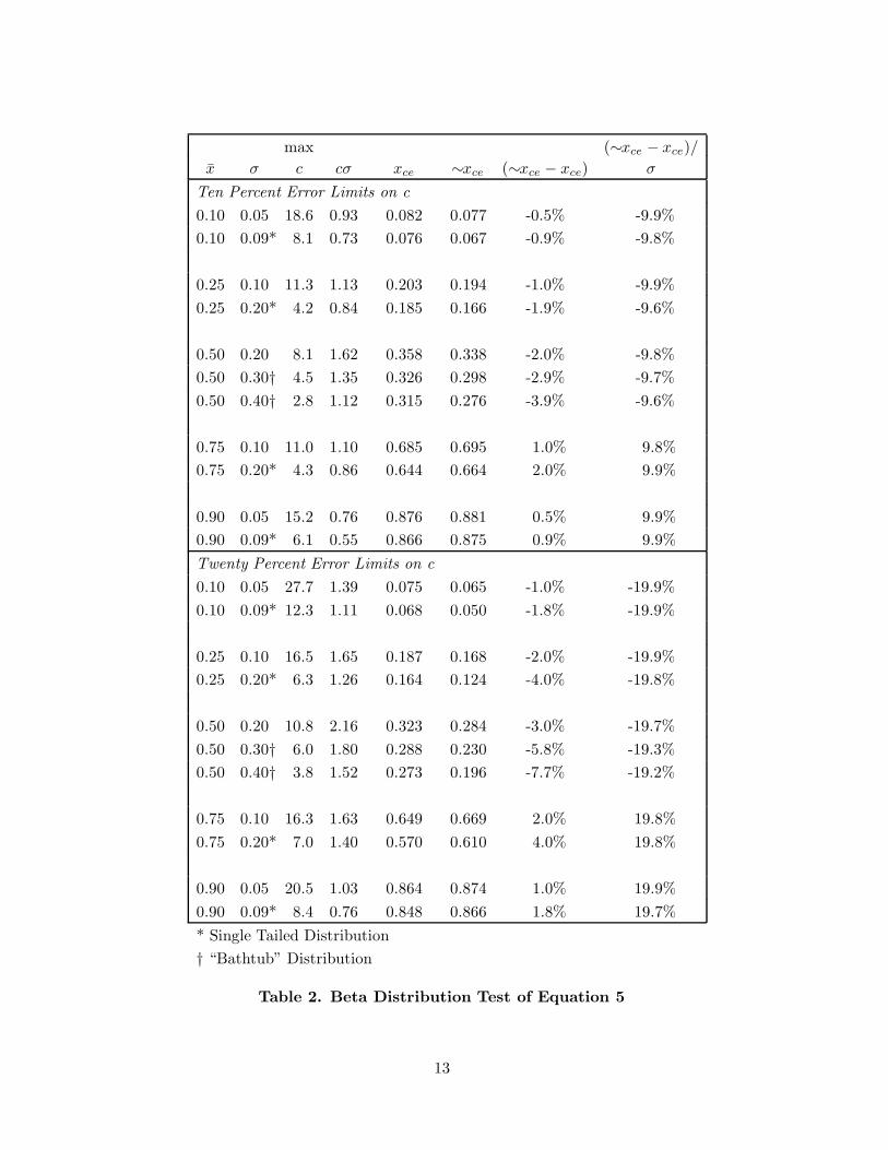
In Table 2, the first column gives the exact expected value of the beta distribu-tion over x, σ is the exact standard deviation, c is the risk aversion coefficient, cσis the product of c and the standard deviation, xce is the exact certainty equivalentfor the beta distribution, ∼xce is the approximate certainty equivalent calculatedusing Equation 5, and the last two columns show the differences between the exactand approximate certainty equivalents as a percentage of the range (from 0 to 1)and standard deviation of the beta distribution.

The upper half of Table 2 give the maximum values of c for which the error usingEquation 5 is less than ten percent of the standard deviation of the distribution forvarious combinations of expected values and standard deviations, while the lowerhalf of the table gives the maximum values of c for which the error is less thantwenty percent of the standard deviation. (As in Table 1, these maximum valuesare in the column labeled “max c.”) This table shows that Equation 5 is accurate formany values of c likely to be assessed in practice for a wide range of shapes for thebeta distribution. Many of the beta distributions for which results are presented areextreme cases that are not at all “normal-like.” Entries in Table 2 marked with oneasterisk are one-tailed distributions with a maximum at either x = 0 or x = 1, whileentries marked with two asterisks have a “bathtub” shape where the distributionincreases as x = 0 and x = 1 are approached. Even with such skewed distributions,Table 2 shows that Equation 5 is accurate for practically useful values for c.

The results in Tables 1 and 2 can be summarized as follows: For the twodistributions studied, Equation 5 is accurate even for probability distributions overx which are not very “normal” in shape. Some cases shown in the tables are moreskewed than most situations of interest in practice. Therefore, the fact that theapproximation is accurate in these cases indicates that it may be accurate in manypractical situations.

Acknowledgment

James L. Corner, Donald L. Keefer, and Jeffrey S. Stonebraker provided valu-able comments on this paper.

References

Drake, A. W. 1967. Fundamentals of Applied Probability Theory, McGraw-Hill, NewYork.

Howard, R. A. 1988. Decision Analysis: Practice and Promise. Management Sci-ence, 34, 679–695.

Keeney, R. L., and Raiffa, H. 1976. Decisions With Multiple Objectives: Preferencesand Value Tradeoffs, Wiley, New York.

McNamee, P., and Celona, J. 1990. Decision Analysis with Supertree, Second Edi-tion, Scientific Press, South San Francisco, CA.

11

max (∼xrp − xrp)/

Range p(x∗) c σ cσ xrp ∼xrp Range σ

Ten Percent Error Limits on c

0.25 0.2 6.6 0.100 0.66 0.023 0.033 3.9% 9.7%

0.25 0.4 7.7 0.122 0.94 0.046 0.058 4.8% 9.8%

0.25 0.6 12.5 0.122 1.53 0.082 0.094 4.8% 9.8%

0.25 0.8 6.7 0.100 0.67 0.043 0.034 -3.9% -9.7%

0.50 0.2 3.3 0.200 0.66 0.047 0.066 3.9% 9.7%

0.50 0.4 3.8 0.245 0.93 0.091 0.114 4.7% 9.6%

0.50 0.6 6.2 0.245 1.52 0.163 0.186 4.6% 9.5%

0.50 0.8 3.3 0.200 0.66 0.085 0.066 -3.8% -9.5%

0.75 0.2 2.2 0.300 0.66 0.070 0.099 3.9% 9.7%

0.75 0.4 2.5 0.367 0.92 0.135 0.169 4.6% 9.3%

0.75 0.6 4.1 0.367 1.51 0.243 0.277 4.5% 9.2%

0.75 0.8 2.2 0.300 0.66 0.128 0.099 -3.8% -9.5%

Twenty Percent Error Limits on c

0.25 0.2 9.9 0.100 0.99 0.030 0.050 8.0% 19.9%

0.25 0.4 10.8 0.122 1.32 0.057 0.081 9.7% 19.8%

0.25 0.6 15.7 0.122 1.92 0.093 0.118 9.7% 19.8%

0.25 0.8 11.3 0.100 1.13 0.076 0.057 -8.0% -19.9%

0.50 0.2 4.9 0.200 0.98 0.059 0.098 7.8% 19.6%

0.50 0.4 5.4 0.245 1.32 0.114 0.162 9.7% 19.8%

0.50 0.6 7.8 0.245 1.91 0.186 0.234 9.5% 19.4%

0.50 0.8 5.6 0.200 1.12 0.151 0.112 -7.9% -19.7%

0.75 0.2 3.3 0.300 0.99 0.089 0.149 8.0% 19.9%

0.75 0.4 3.6 0.367 1.32 0.170 0.243 9.7% 19.8%

0.75 0.6 5.2 0.367 1.91 0.280 0.351 9.5% 19.4%

0.75 0.8 3.7 0.300 1.11 0.225 0.167 -7.8% -19.6%

Table 1. Two-Fork Lottery Test of Equation 5

12

max (∼xce − xce)/

x̄ σ c cσ xce ∼xce (∼xce − xce) σ

Ten Percent Error Limits on c

0.10 0.05 18.6 0.93 0.082 0.077 -0.5% -9.9%

0.10 0.09* 8.1 0.73 0.076 0.067 -0.9% -9.8%

0.25 0.10 11.3 1.13 0.203 0.194 -1.0% -9.9%

0.25 0.20* 4.2 0.84 0.185 0.166 -1.9% -9.6%

0.50 0.20 8.1 1.62 0.358 0.338 -2.0% -9.8%

0.50 0.30† 4.5 1.35 0.326 0.298 -2.9% -9.7%

0.50 0.40† 2.8 1.12 0.315 0.276 -3.9% -9.6%

0.75 0.10 11.0 1.10 0.685 0.695 1.0% 9.8%

0.75 0.20* 4.3 0.86 0.644 0.664 2.0% 9.9%

0.90 0.05 15.2 0.76 0.876 0.881 0.5% 9.9%

0.90 0.09* 6.1 0.55 0.866 0.875 0.9% 9.9%

Twenty Percent Error Limits on c

0.10 0.05 27.7 1.39 0.075 0.065 -1.0% -19.9%

0.10 0.09* 12.3 1.11 0.068 0.050 -1.8% -19.9%

0.25 0.10 16.5 1.65 0.187 0.168 -2.0% -19.9%

0.25 0.20* 6.3 1.26 0.164 0.124 -4.0% -19.8%

0.50 0.20 10.8 2.16 0.323 0.284 -3.0% -19.7%

0.50 0.30† 6.0 1.80 0.288 0.230 -5.8% -19.3%

0.50 0.40† 3.8 1.52 0.273 0.196 -7.7% -19.2%

0.75 0.10 16.3 1.63 0.649 0.669 2.0% 19.8%

0.75 0.20* 7.0 1.40 0.570 0.610 4.0% 19.8%

0.90 0.05 20.5 1.03 0.864 0.874 1.0% 19.9%

0.90 0.09* 8.4 0.76 0.848 0.866 1.8% 19.7%

* Single Tailed Distribution

† “Bathtub” Distribution

Table 2. Beta Distribution Test of Equation 5

13

Pratt, J. W. 1964. Risk Aversion in the Small and in the Large. Econometrica, 32,122–136.

Pratt, J. W., H. Raiffa and R. O. Schlaifer. 1964. The Foundations of DecisionUnder Uncertainty: An Elementary Exposition. Journal of the American Sta-tistical Association 59, 353–375.

14

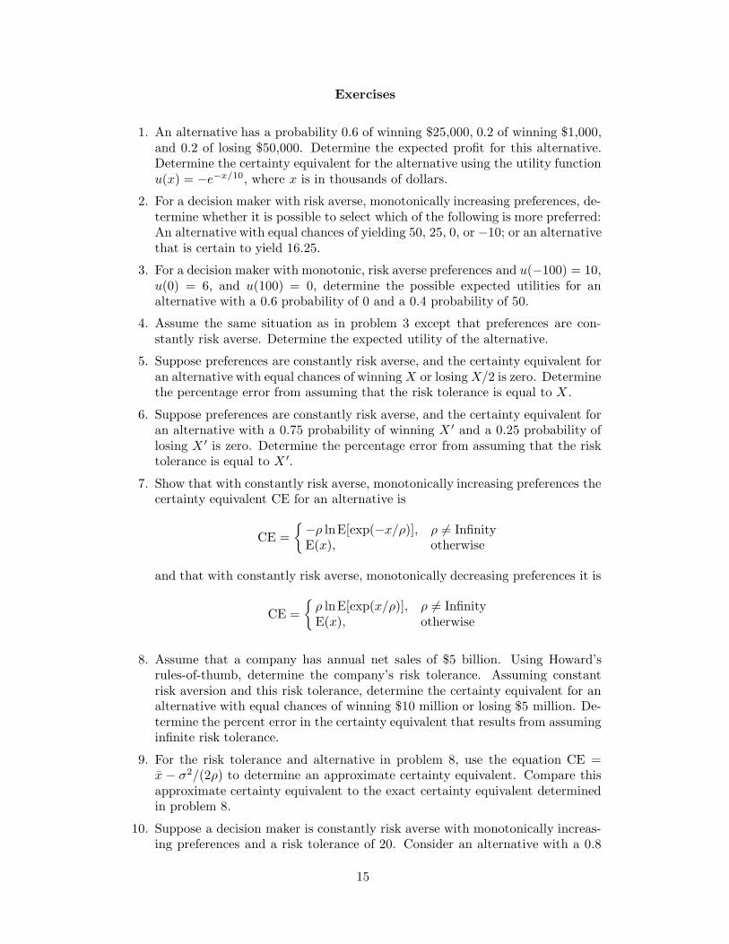
Exercises

1. An alternative has a probability 0.6 of winning $25,000, 0.2 of winning $1,000,and 0.2 of losing $50,000. Determine the expected profit for this alternative.Determine the certainty equivalent for the alternative using the utility functionu(x) = −e−x/10, where x is in thousands of dollars.

2. For a decision maker with risk averse, monotonically increasing preferences, de-termine whether it is possible to select which of the following is more preferred:An alternative with equal chances of yielding 50, 25, 0, or −10; or an alternativethat is certain to yield 16.25.

3. For a decision maker with monotonic, risk averse preferences and u(−100) = 10,u(0) = 6, and u(100) = 0, determine the possible expected utilities for analternative with a 0.6 probability of 0 and a 0.4 probability of 50.

4. Assume the same situation as in problem 3 except that preferences are con-stantly risk averse. Determine the expected utility of the alternative.

5. Suppose preferences are constantly risk averse, and the certainty equivalent foran alternative with equal chances of winning X or losing X/2 is zero. Determinethe percentage error from assuming that the risk tolerance is equal to X .

6. Suppose preferences are constantly risk averse, and the certainty equivalent foran alternative with a 0.75 probability of winning X ′ and a 0.25 probability oflosing X ′ is zero. Determine the percentage error from assuming that the risktolerance is equal to X ′.

7. Show that with constantly risk averse, monotonically increasing preferences thecertainty equivalent CE for an alternative is

CE =

{

−ρ lnE[exp(−x/ρ)], ρ 6= InfinityE(x), otherwise

and that with constantly risk averse, monotonically decreasing preferences it is

CE =

{

ρ lnE[exp(x/ρ)], ρ 6= InfinityE(x), otherwise

8. Assume that a company has annual net sales of $5 billion. Using Howard’srules-of-thumb, determine the company’s risk tolerance. Assuming constantrisk aversion and this risk tolerance, determine the certainty equivalent for analternative with equal chances of winning $10 million or losing $5 million. De-termine the percent error in the certainty equivalent that results from assuminginfinite risk tolerance.

9. For the risk tolerance and alternative in problem 8, use the equation CE =x̄ − σ2/(2ρ) to determine an approximate certainty equivalent. Compare thisapproximate certainty equivalent to the exact certainty equivalent determinedin problem 8.

10. Suppose a decision maker is constantly risk averse with monotonically increas-ing preferences and a risk tolerance of 20. Consider an alternative with a 0.8

15

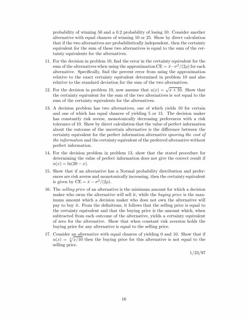
probability of winning 50 and a 0.2 probability of losing 10. Consider anotheralternative with equal chances of winning 10 or 25. Show by direct calculationthat if the two alternatives are probabilistically independent, then the certaintyequivalent for the sum of these two alternatives is equal to the sum of the cer-tainty equivalents for the alternatives.

11. For the decision in problem 10, find the error in the certainty equivalent for thesum of the alternatives when using the approximation CE = x̄−σ2/(2ρ) for eachalternative. Specifically, find the percent error from using the approximationrelative to the exact certainty equivalent determined in problem 10 and alsorelative to the standard deviation for the sum of the two alternatives.

12. For the decision in problem 10, now assume that u(x) =√

x + 10. Show thatthe certainty equivalent for the sum of the two alternatives is not equal to thesum of the certainty equivalents for the alternatives.

13. A decision problem has two alternatives, one of which yields 10 for certainand one of which has equal chances of yielding 5 or 15. The decision makerhas constantly risk averse, monotonically decreasing preferences with a risktolerance of 10. Show by direct calculation that the value of perfect informationabout the outcome of the uncertain alternative is the difference between thecertainty equivalent for the perfect information alternative ignoring the cost ofthe information and the certainty equivalent of the preferred alternative withoutperfect information.

14. For the decision problem in problem 13, show that the stated procedure fordetermining the value of perfect information does not give the correct result ifu(x) = ln(20− x).

15. Show that if an alternative has a Normal probability distribution and prefer-ences are risk averse and monotonically increasing, then the certainty equivalentis given by CE = x̄ − σ2/(2ρ).

16. The selling price of an alternative is the minimum amount for which a decisionmaker who owns the alternative will sell it, while the buying price is the max-imum amount which a decision maker who does not own the alternative willpay to buy it. From the definitions, it follows that the selling price is equal tothe certainty equivalent and that the buying price is the amount which, whensubtracted from each outcome of the alternative, yields a certainty equivalentof zero for the alternative. Show that when constant risk aversion holds thebuying price for any alternative is equal to the selling price.

17. Consider an alternative with equal chances of yielding 0 and 10. Show that ifu(x) = 3

√

x/10 then the buying price for this alternative is not equal to theselling price.

1/23/97

16

Appendix A. Two Fundamental Theorems

This appendix presents the axioms of consistent choice and two fundamentaltheorems which result from these axioms. In this appendix, the symbol “�” means“is preferred to,” and the consequences of a decision are designated c1, c2, . . . , cn.Note that these consequences may themselves be uncertain alternatives. Theseaxioms assume that probabilities exist and that the rules of probability apply. Pratt,Raiffa, and Schlaifer (1964) present a more extensive set of axioms which developsprobability from first principles. Here are the axioms of consistent choice:

1. (Transitivity) If ci � cj and cj � ck, then ci � ck.

2. (Reduction) If the standard rules of probability can be used to show that twoalternatives have the same probability for each ci, then the two alternatives areequally preferred.

3. (Continuity) If ci � cj � ck, then there is a p such that an alternative witha probability p of yielding ci and a probability 1 − p of yielding ck is equallypreferred to cj .

4. (Substitution) If two consequences are equally preferred, then one can be sub-stituted for the other in any decision without changing the preference orderingof alternatives.

5. (Monotonicity) For two alternatives which each yield either ci or cj whereci � cj , then the first alternative is preferred to the second if it has a higherprobability of yielding ci.

If these conditions hold, then it is possible to prove the following theorem.

Theorem A-1 (Expected Utility). If the axioms of consistent choice hold, thenthere exists a function u(ci) such that alternative A is preferred to alternative B if

n∑

i=1

p(ci|A)u(ci) >

n∑

i=1

p(ci|B)u(ci) (A − 1)

where p(ci|A) is the probability of ci if A is selected, and p(ci|B) is the probabilityof ci if B is selected.

Proof. The following steps demonstrate the desired result:

1. Using the Transitivity Axiom, the consequences can be rank-ordered in terms ofpreferability. Suppose the consequences are labeled so that c1 � c2 � · · · � cn.

2. By the Reduction Axiom, any uncertain alternative has an equally preferred al-ternative which directly yields the outcomes c1, c2, . . . , cn. Suppose the equallypreferred alternative for A has probabilities p(c1|A), p(c2|A), . . . , p(cn|A) ofyielding c1, c2, . . . , cn respectively, and the equally preferred alternative for Bhas probabilities p(c1|B), p(c2|B), . . . , p(cn|B) of yielding c1, c2, . . . , cn. Thenby the Substitution Axiom, the original alternatives can be replaced by theirequally preferred reduced equivalents. Make this replacement.

3. By the Continuity Axiom, there is a number u(ci) such that ci is equally pre-ferred to an alternative with a probability u(ci) of yielding c1 and a probability

17

1 − u(ci) of yielding cn. Thus, by the Substitution Axiom, each ci can bereplaced by the equally preferred alternative which has a probability u(ci) ofyielding c1 and a probability 1 − u(ci) of yielding cn. Make this substitution.

5. By the Reduction Axiom, A is equally preferred to an alternative with a prob-ability

∑ni=1 p(ci|A)u(ci) of yielding c1 and a probability 1−∑n

i=1 p(ci|A)u(ci)of yielding cn. Similarly, B is equally preferred to an alternative with a proba-bility

∑ni=1 p(ci|B)u(ci) of yielding c1 and a probability 1 − ∑n

i=1 p(ci|B)u(ci)of yielding cn. Thus, by the Substitution Axiom, A and B can be replaced bythese alternatives which have outcomes which only include c1 and cn. Makethis substitution.

6. Thus, by the Monotonicity Axiom, A � B if

n∑

i=1

p(ci|A)u(ci) >

n∑

i=1

p(ci|B)u(ci).

This is the relationship in Equation A-1.

The function u(ci) is called a utility function, and the decision criterion in The-orem A-1 says that expected utility must be used as a decision criterion if the axiomsof consistent choice are to be obeyed. These axioms were originally postulated as amodel of unaided human decision making behavior. Many experiments have beendone to test whether unaided human decision making naturally obeys the axioms.The results have shown that unaided human decision making does not obey theaxioms of consistent choice. This has led to some questioning of whether the axiomsare a good basis for decision analysis procedures, and a number of alternative axiomsets have been developed to better describe unaided human decision making.

However, there is a difference between describing how unaided decision makingprocesses work and using analysis to make better decisions. Our focus here is onmaking better decisions. From this perspective, it is difficult to argue with theaxioms of consistent choice. Each is reasonable, and it is hard to give any of themup as logical principles that we would want our reasoning to obey.

On a more practical level, we are all aware of limitations in human reasoning.Very few of us would trust ourselves to accurately add up a column of 100 numbersin our head. Many decisions under uncertainty are more complex than adding up100 numbers. Why should we trust our unaided reasoning processes to be moreaccurate at analyzing these decisions than at adding 100 numbers? Thus, the factthat unaided decision making does not obey the axioms of consistent choice is nota convincing argument that these axioms should not be used as a basis for decisionmaking.

There is another theorem related to utility functions that is useful. The proofof Theorem A-1 shows that u(ci) must be between 0 and 1 since it is defined asa probability. However, it is not necessary that all utility functions be between 0and 1, as the following theorem demonstrates.

18

Theorem A-2 (Linear Transformation). Given a utility function u(ci), then an-other function u′(ci) is guaranteed to give the same ranking of alternatives if andonly if

u′(ci) = au(ci) + b (A − 2)

for some constants a > 0 and b.

Proof. Suppose that∑n

i=1 p(ci|A)u(ci) >∑n

i=1 p(ci|B)u(ci). Then, it is also truethat a

∑ni=1 p(ci|A)u(ci) > a

∑ni=1 p(ci|B)u(ci) for any constant a > 0, and hence

a∑n

i=1 p(ci|A)u(ci) + b > a∑n

i=1 p(ci|B)u(ci) + b for any constant b.

However, since a∑n

i=1 p(ci|A)u(ci) + b =∑n

i=1 p(ci|A)[au(ci) + b] anda

∑ni=1 p(ci|B)u(ci) + b =

∑ni=1 p(ci|B)[au(ci) + b], which is the same as

n∑

i=1

p(ci|A)u′(ci) >

n∑

i=1

p(ci|B)u′(ci),

then the desired result is demonstrated.

19

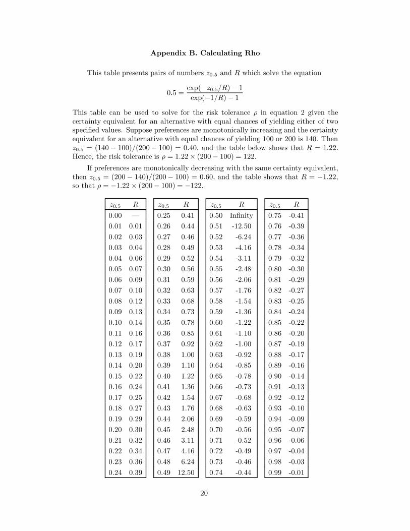
Appendix B. Calculating Rho

This table presents pairs of numbers z0.5 and R which solve the equation

0.5 =exp(−z0.5/R)− 1

exp(−1/R) − 1

This table can be used to solve for the risk tolerance ρ in equation 2 given thecertainty equivalent for an alternative with equal chances of yielding either of twospecified values. Suppose preferences are monotonically increasing and the certaintyequivalent for an alternative with equal chances of yielding 100 or 200 is 140. Thenz0.5 = (140 − 100)/(200− 100) = 0.40, and the table below shows that R = 1.22.Hence, the risk tolerance is ρ = 1.22× (200− 100) = 122.

If preferences are monotonically decreasing with the same certainty equivalent,then z0.5 = (200 − 140)/(200− 100) = 0.60, and the table shows that R = −1.22,so that ρ = −1.22 × (200− 100) = −122.

z0.5 R z0.5 R z0.5 R z0.5 R

0.00 — 0.25 0.41 0.50 Infinity 0.75 -0.41

0.01 0.01 0.26 0.44 0.51 -12.50 0.76 -0.39

0.02 0.03 0.27 0.46 0.52 -6.24 0.77 -0.36

0.03 0.04 0.28 0.49 0.53 -4.16 0.78 -0.34

0.04 0.06 0.29 0.52 0.54 -3.11 0.79 -0.32

0.05 0.07 0.30 0.56 0.55 -2.48 0.80 -0.30

0.06 0.09 0.31 0.59 0.56 -2.06 0.81 -0.29

0.07 0.10 0.32 0.63 0.57 -1.76 0.82 -0.27

0.08 0.12 0.33 0.68 0.58 -1.54 0.83 -0.25

0.09 0.13 0.34 0.73 0.59 -1.36 0.84 -0.24

0.10 0.14 0.35 0.78 0.60 -1.22 0.85 -0.22

0.11 0.16 0.36 0.85 0.61 -1.10 0.86 -0.20

0.12 0.17 0.37 0.92 0.62 -1.00 0.87 -0.19

0.13 0.19 0.38 1.00 0.63 -0.92 0.88 -0.17

0.14 0.20 0.39 1.10 0.64 -0.85 0.89 -0.16

0.15 0.22 0.40 1.22 0.65 -0.78 0.90 -0.14

0.16 0.24 0.41 1.36 0.66 -0.73 0.91 -0.13

0.17 0.25 0.42 1.54 0.67 -0.68 0.92 -0.12

0.18 0.27 0.43 1.76 0.68 -0.63 0.93 -0.10

0.19 0.29 0.44 2.06 0.69 -0.59 0.94 -0.09

0.20 0.30 0.45 2.48 0.70 -0.56 0.95 -0.07

0.21 0.32 0.46 3.11 0.71 -0.52 0.96 -0.06

0.22 0.34 0.47 4.16 0.72 -0.49 0.97 -0.04

0.23 0.36 0.48 6.24 0.73 -0.46 0.98 -0.03

0.24 0.39 0.49 12.50 0.74 -0.44 0.99 -0.01

20

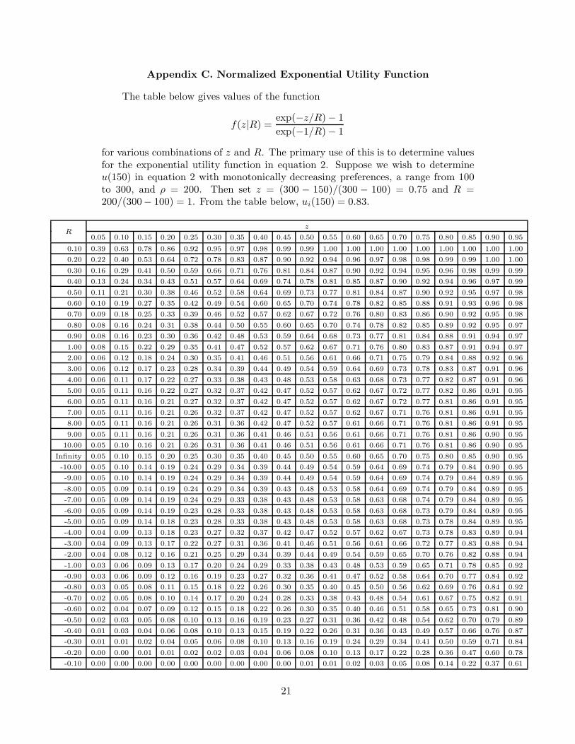
Appendix C. Normalized Exponential Utility Function

The table below gives values of the function

f(z|R) =exp(−z/R)− 1

exp(−1/R)− 1

for various combinations of z and R. The primary use of this is to determine valuesfor the exponential utility function in equation 2. Suppose we wish to determineu(150) in equation 2 with monotonically decreasing preferences, a range from 100to 300, and ρ = 200. Then set z = (300 − 150)/(300 − 100) = 0.75 and R =200/(300− 100) = 1. From the table below, ui(150) = 0.83.

zR

0.05 0.10 0.15 0.20 0.25 0.30 0.35 0.40 0.45 0.50 0.55 0.60 0.65 0.70 0.75 0.80 0.85 0.90 0.95

0.10 0.39 0.63 0.78 0.86 0.92 0.95 0.97 0.98 0.99 0.99 1.00 1.00 1.00 1.00 1.00 1.00 1.00 1.00 1.00

0.20 0.22 0.40 0.53 0.64 0.72 0.78 0.83 0.87 0.90 0.92 0.94 0.96 0.97 0.98 0.98 0.99 0.99 1.00 1.00

0.30 0.16 0.29 0.41 0.50 0.59 0.66 0.71 0.76 0.81 0.84 0.87 0.90 0.92 0.94 0.95 0.96 0.98 0.99 0.99

0.40 0.13 0.24 0.34 0.43 0.51 0.57 0.64 0.69 0.74 0.78 0.81 0.85 0.87 0.90 0.92 0.94 0.96 0.97 0.99

0.50 0.11 0.21 0.30 0.38 0.46 0.52 0.58 0.64 0.69 0.73 0.77 0.81 0.84 0.87 0.90 0.92 0.95 0.97 0.98

0.60 0.10 0.19 0.27 0.35 0.42 0.49 0.54 0.60 0.65 0.70 0.74 0.78 0.82 0.85 0.88 0.91 0.93 0.96 0.98

0.70 0.09 0.18 0.25 0.33 0.39 0.46 0.52 0.57 0.62 0.67 0.72 0.76 0.80 0.83 0.86 0.90 0.92 0.95 0.98

0.80 0.08 0.16 0.24 0.31 0.38 0.44 0.50 0.55 0.60 0.65 0.70 0.74 0.78 0.82 0.85 0.89 0.92 0.95 0.97

0.90 0.08 0.16 0.23 0.30 0.36 0.42 0.48 0.53 0.59 0.64 0.68 0.73 0.77 0.81 0.84 0.88 0.91 0.94 0.97

1.00 0.08 0.15 0.22 0.29 0.35 0.41 0.47 0.52 0.57 0.62 0.67 0.71 0.76 0.80 0.83 0.87 0.91 0.94 0.97

2.00 0.06 0.12 0.18 0.24 0.30 0.35 0.41 0.46 0.51 0.56 0.61 0.66 0.71 0.75 0.79 0.84 0.88 0.92 0.96

3.00 0.06 0.12 0.17 0.23 0.28 0.34 0.39 0.44 0.49 0.54 0.59 0.64 0.69 0.73 0.78 0.83 0.87 0.91 0.96

4.00 0.06 0.11 0.17 0.22 0.27 0.33 0.38 0.43 0.48 0.53 0.58 0.63 0.68 0.73 0.77 0.82 0.87 0.91 0.96

5.00 0.05 0.11 0.16 0.22 0.27 0.32 0.37 0.42 0.47 0.52 0.57 0.62 0.67 0.72 0.77 0.82 0.86 0.91 0.95

6.00 0.05 0.11 0.16 0.21 0.27 0.32 0.37 0.42 0.47 0.52 0.57 0.62 0.67 0.72 0.77 0.81 0.86 0.91 0.95

7.00 0.05 0.11 0.16 0.21 0.26 0.32 0.37 0.42 0.47 0.52 0.57 0.62 0.67 0.71 0.76 0.81 0.86 0.91 0.95

8.00 0.05 0.11 0.16 0.21 0.26 0.31 0.36 0.42 0.47 0.52 0.57 0.61 0.66 0.71 0.76 0.81 0.86 0.91 0.95

9.00 0.05 0.11 0.16 0.21 0.26 0.31 0.36 0.41 0.46 0.51 0.56 0.61 0.66 0.71 0.76 0.81 0.86 0.90 0.95

10.00 0.05 0.10 0.16 0.21 0.26 0.31 0.36 0.41 0.46 0.51 0.56 0.61 0.66 0.71 0.76 0.81 0.86 0.90 0.95

Infinity 0.05 0.10 0.15 0.20 0.25 0.30 0.35 0.40 0.45 0.50 0.55 0.60 0.65 0.70 0.75 0.80 0.85 0.90 0.95

-10.00 0.05 0.10 0.14 0.19 0.24 0.29 0.34 0.39 0.44 0.49 0.54 0.59 0.64 0.69 0.74 0.79 0.84 0.90 0.95

-9.00 0.05 0.10 0.14 0.19 0.24 0.29 0.34 0.39 0.44 0.49 0.54 0.59 0.64 0.69 0.74 0.79 0.84 0.89 0.95

-8.00 0.05 0.09 0.14 0.19 0.24 0.29 0.34 0.39 0.43 0.48 0.53 0.58 0.64 0.69 0.74 0.79 0.84 0.89 0.95

-7.00 0.05 0.09 0.14 0.19 0.24 0.29 0.33 0.38 0.43 0.48 0.53 0.58 0.63 0.68 0.74 0.79 0.84 0.89 0.95

-6.00 0.05 0.09 0.14 0.19 0.23 0.28 0.33 0.38 0.43 0.48 0.53 0.58 0.63 0.68 0.73 0.79 0.84 0.89 0.95

-5.00 0.05 0.09 0.14 0.18 0.23 0.28 0.33 0.38 0.43 0.48 0.53 0.58 0.63 0.68 0.73 0.78 0.84 0.89 0.95

-4.00 0.04 0.09 0.13 0.18 0.23 0.27 0.32 0.37 0.42 0.47 0.52 0.57 0.62 0.67 0.73 0.78 0.83 0.89 0.94

-3.00 0.04 0.09 0.13 0.17 0.22 0.27 0.31 0.36 0.41 0.46 0.51 0.56 0.61 0.66 0.72 0.77 0.83 0.88 0.94

-2.00 0.04 0.08 0.12 0.16 0.21 0.25 0.29 0.34 0.39 0.44 0.49 0.54 0.59 0.65 0.70 0.76 0.82 0.88 0.94

-1.00 0.03 0.06 0.09 0.13 0.17 0.20 0.24 0.29 0.33 0.38 0.43 0.48 0.53 0.59 0.65 0.71 0.78 0.85 0.92

-0.90 0.03 0.06 0.09 0.12 0.16 0.19 0.23 0.27 0.32 0.36 0.41 0.47 0.52 0.58 0.64 0.70 0.77 0.84 0.92

-0.80 0.03 0.05 0.08 0.11 0.15 0.18 0.22 0.26 0.30 0.35 0.40 0.45 0.50 0.56 0.62 0.69 0.76 0.84 0.92

-0.70 0.02 0.05 0.08 0.10 0.14 0.17 0.20 0.24 0.28 0.33 0.38 0.43 0.48 0.54 0.61 0.67 0.75 0.82 0.91

-0.60 0.02 0.04 0.07 0.09 0.12 0.15 0.18 0.22 0.26 0.30 0.35 0.40 0.46 0.51 0.58 0.65 0.73 0.81 0.90

-0.50 0.02 0.03 0.05 0.08 0.10 0.13 0.16 0.19 0.23 0.27 0.31 0.36 0.42 0.48 0.54 0.62 0.70 0.79 0.89

-0.40 0.01 0.03 0.04 0.06 0.08 0.10 0.13 0.15 0.19 0.22 0.26 0.31 0.36 0.43 0.49 0.57 0.66 0.76 0.87

-0.30 0.01 0.01 0.02 0.04 0.05 0.06 0.08 0.10 0.13 0.16 0.19 0.24 0.29 0.34 0.41 0.50 0.59 0.71 0.84

-0.20 0.00 0.00 0.01 0.01 0.02 0.02 0.03 0.04 0.06 0.08 0.10 0.13 0.17 0.22 0.28 0.36 0.47 0.60 0.78

-0.10 0.00 0.00 0.00 0.00 0.00 0.00 0.00 0.00 0.00 0.01 0.01 0.02 0.03 0.05 0.08 0.14 0.22 0.37 0.61

21

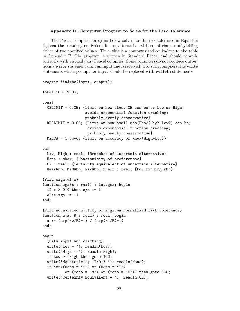
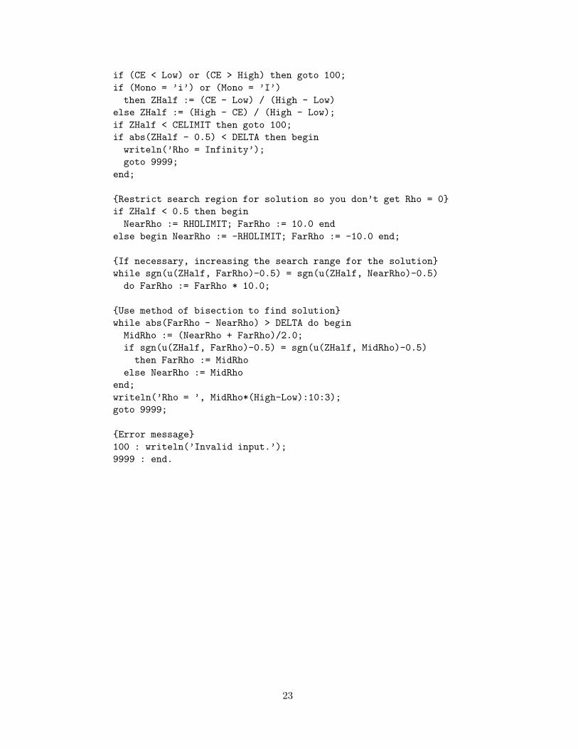
Appendix D. Computer Program to Solve for the Risk Tolerance

The Pascal computer program below solves for the risk tolerance in Equation2 given the certainty equivalent for an alternative with equal chances of yieldingeither of two specified values. Thus, this is a computerized equivalent to the tablein Appendix B. The program is written in Standard Pascal and should compilecorrectly with virtually any Pascal compiler. Some compilers do not produce outputfrom a write statement until an input line is received. For such compilers, the write

statements which prompt for input should be replaced with writeln statements.

program findrho(input, output);

label 100, 9999;

const

CELIMIT = 0.05; {Limit on how close CE can be to Low or High;

avoids exponential function crashing;

probably overly conservative}

RHOLIMIT = 0.05; {Limit on how small abs(Rho/(High-Low)) can be;

avoids exponential function crashing;

probably overly conservative}

DELTA = 1.0e-6; {Limit on accuracy of Rho/(High-Low)}

var

Low, High : real; {Branches of uncertain alternative}

Mono : char; {Monotonicity of preferences}

CE : real; {Certainty equivalent of uncertain alternative}

NearRho, MidRho, FarRho, ZHalf : real; {For finding rho}

{Find sign of x}

function sgn(x : real) : integer; begin

if x > 0.0 then sgn := 1

else sgn := -1

end;

{Find normalized utility of z given normalized risk tolerance}

function u(z, R : real) : real; begin

u := (exp(-z/R)-1) / (exp(-1/R)-1)

end;

begin

{Data input and checking}

write(’Low = ’); readln(Low);

write(’High = ’); readln(High);

if Low >= High then goto 100;

write(’Monotonicity (I/D)? ’); readln(Mono);

if not((Mono = ’i’) or (Mono = ’I’)

or (Mono = ’d’) or (Mono = ’D’)) then goto 100;

write(’Certainty Equivalent = ’); readln(CE);

22

if (CE < Low) or (CE > High) then goto 100;

if (Mono = ’i’) or (Mono = ’I’)

then ZHalf := (CE - Low) / (High - Low)

else ZHalf := (High - CE) / (High - Low);

if ZHalf < CELIMIT then goto 100;

if abs(ZHalf - 0.5) < DELTA then begin

writeln(’Rho = Infinity’);

goto 9999;

end;

{Restrict search region for solution so you don’t get Rho = 0}

if ZHalf < 0.5 then begin

NearRho := RHOLIMIT; FarRho := 10.0 end

else begin NearRho := -RHOLIMIT; FarRho := -10.0 end;

{If necessary, increasing the search range for the solution}

while sgn(u(ZHalf, FarRho)-0.5) = sgn(u(ZHalf, NearRho)-0.5)

do FarRho := FarRho * 10.0;

{Use method of bisection to find solution}

while abs(FarRho - NearRho) > DELTA do begin

MidRho := (NearRho + FarRho)/2.0;

if sgn(u(ZHalf, FarRho)-0.5) = sgn(u(ZHalf, MidRho)-0.5)

then FarRho := MidRho

else NearRho := MidRho

end;

writeln(’Rho = ’, MidRho*(High-Low):10:3);

goto 9999;

{Error message}

100 : writeln(’Invalid input.’);

9999 : end.

23