Embed Size (px)
Citation preview
Copyright © 2005 Paul S. Steif 1
Notes on Elasticity and Finite Element Analysis
Paul S. Steif Department of Mechanical Engineering
Carnegie Mellon University All mechanical and civil engineering students take at least one course in mechanics of materials. For many students though, this is their last formal course in the mechanics of deforming solid bodies. Yet, it is increasingly likely for practicing engineers to be called upon to do finite element analysis (FEA) as part of their engineering activities. A thorough grounding in the theory of linear elasticity which underlies FEA, while advantageous, is less and less common. These notes attempt to enable students with only a background in mechanics of materials to be more effective users of FEA. These notes are divided into the following Chapters: 1. Essential Variables in Elasticity The key quantities of elasticity - displacements, strains and stresses - are defined so as to give the reader a physical intuitive feel for them. 2. Formulation of an elasticity problem The essential elements in using elasticity are covered, including the stress-strain law, boundary conditions, and the field equations of equilibrium and compatibility. 3. Finite Element Method The major steps in carrying out a finite element analysis are reviewed and their relations to elements of elasticity are pointed out. 4. Stress Concentrations and Singularities Two major pitfalls in finite element analysis – stress concentrations and singularities – are discussed. Since, displacement constraints so often lead to singularities, the means of applying minimal displacements to constrain a body which is otherwise under applied forces is also covered. 5. Examining the Results of FEA Various methods used by experienced analysts to test the accuracy of finite element results are reviewed, including the use approximate analyses based on mechanics of materials.
Copyright © 2005 Paul S. Steif 2
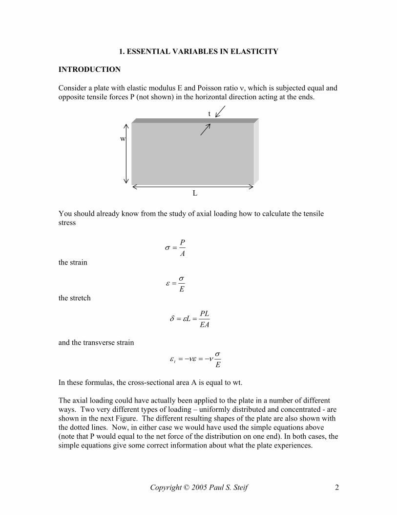
1. ESSENTIAL VARIABLES IN ELASTICITY INTRODUCTION Consider a plate with elastic modulus E and Poisson ratio ν, which is subjected equal and opposite tensile forces P (not shown) in the horizontal direction acting at the ends.
Figure of plate under tension You should already know from the study of axial loading how to calculate the tensile stress
the strain
the stretch
and the transverse strain
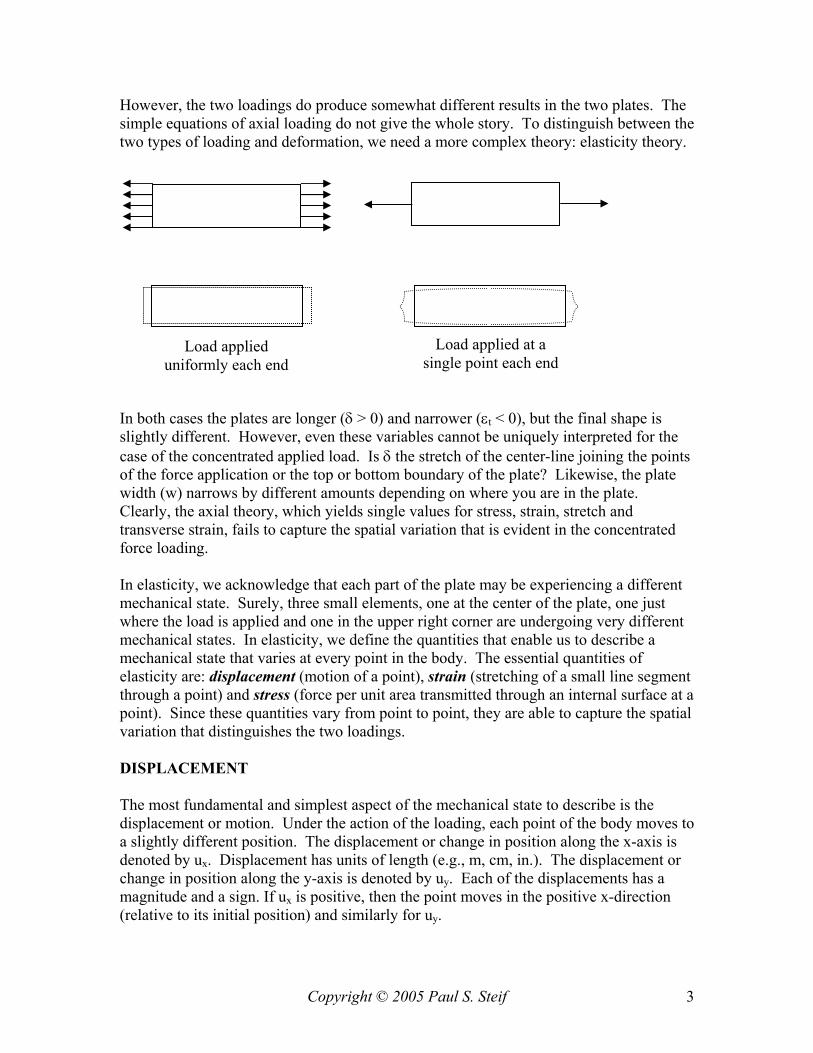
In these formulas, the cross-sectional area A is equal to wt. The axial loading could have actually been applied to the plate in a number of different ways. Two very different types of loading – uniformly distributed and concentrated - are shown in the next Figure. The different resulting shapes of the plate are also shown with the dotted lines. Now, in either case we would have used the simple equations above (note that P would equal to the net force of the distribution on one end). In both cases, the simple equations give some correct information about what the plate experiences.
AP
=σ
Eσε =
EAPLL == εδ
Etσννεε −=−=
L
t
w
Copyright © 2005 Paul S. Steif 3
However, the two loadings do produce somewhat different results in the two plates. The simple equations of axial loading do not give the whole story. To distinguish between the two types of loading and deformation, we need a more complex theory: elasticity theory. In both cases the plates are longer (δ > 0) and narrower (εt < 0), but the final shape is slightly different. However, even these variables cannot be uniquely interpreted for the case of the concentrated applied load. Is δ the stretch of the center-line joining the points of the force application or the top or bottom boundary of the plate? Likewise, the plate width (w) narrows by different amounts depending on where you are in the plate. Clearly, the axial theory, which yields single values for stress, strain, stretch and transverse strain, fails to capture the spatial variation that is evident in the concentrated force loading. In elasticity, we acknowledge that each part of the plate may be experiencing a different mechanical state. Surely, three small elements, one at the center of the plate, one just where the load is applied and one in the upper right corner are undergoing very different mechanical states. In elasticity, we define the quantities that enable us to describe a mechanical state that varies at every point in the body. The essential quantities of elasticity are: displacement (motion of a point), strain (stretching of a small line segment through a point) and stress (force per unit area transmitted through an internal surface at a point). Since these quantities vary from point to point, they are able to capture the spatial variation that distinguishes the two loadings. DISPLACEMENT The most fundamental and simplest aspect of the mechanical state to describe is the displacement or motion. Under the action of the loading, each point of the body moves to a slightly different position. The displacement or change in position along the x-axis is denoted by ux. Displacement has units of length (e.g., m, cm, in.). The displacement or change in position along the y-axis is denoted by uy. Each of the displacements has a magnitude and a sign. If ux is positive, then the point moves in the positive x-direction (relative to its initial position) and similarly for uy.
Load applied uniformly each end
Load applied at a single point each end
Copyright © 2005 Paul S. Steif 4
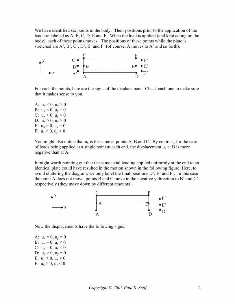
We have identified six points in the body. Their positions prior to the application of the load are labeled as A, B, C, D, E and F. When the load is applied (and kept acting on the body), each of these points moves. The positions of these points while the plate is stretched are A’, B’, C’, D’, E’ and F’ (of course, A moves to A’ and so forth). For each the points, here are the signs of the displacement. Check each one to make sure that it makes sense to you. A: ux < 0, uy > 0 B: ux < 0, uy = 0 C: ux < 0, uy < 0 D: ux > 0, uy > 0 E: ux > 0, uy = 0 F: ux > 0, uy < 0 You might also notice that ux is the same at points A, B and C. By contrast, for the case of loads being applied at a single point at each end, the displacement ux at B is more negative than at A. It might worth pointing out that the same axial loading applied uniformly at the end to an identical plate could have resulted in the motion shown in the following figure. Here, to avoid cluttering the diagram, we only label the final positions D’, E’ and F’. In this case the point A does not move, points B and C move in the negative y direction to B’ and C’ respectively (they move down by different amounts). Now the displacements have the following signs: A: ux = 0, uy = 0 B: ux = 0, uy < 0 C: ux = 0, uy < 0 D: ux > 0, uy = 0 E: ux > 0, uy < 0 F: ux > 0, uy < 0
A A’ B B’
CC’
DD’
E E’
FF’ y
x
A
B
C
D
E
Fy
x D’ E’ F’
Copyright © 2005 Paul S. Steif 5
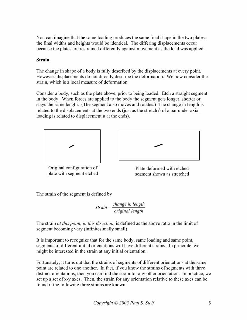
You can imagine that the same loading produces the same final shape in the two plates: the final widths and heights would be identical. The differing displacements occur because the plates are restrained differently against movement as the load was applied. Strain The change in shape of a body is fully described by the displacements at every point. However, displacements do not directly describe the deformation. We now consider the strain, which is a local measure of deformation. Consider a body, such as the plate above, prior to being loaded. Etch a straight segment in the body. When forces are applied to the body the segment gets longer, shorter or stays the same length. (The segment also moves and rotates.) The change in length is related to the displacements at the two ends (just as the stretch δ of a bar under axial loading is related to displacement u at the ends). The strain of the segment is defined by
The strain at this point, in this direction, is defined as the above ratio in the limit of segment becoming very (infinitesimally small). It is important to recognize that for the same body, same loading and same point, segments of different initial orientations will have different strains. In principle, we might be interested in the strain at any initial orientation. Fortunately, it turns out that the strains of segments of different orientations at the same point are related to one another. In fact, if you know the strains of segments with three distinct orientations, then you can find the strain for any other orientation. In practice, we set up a set of x-y axes. Then, the strain for any orientation relative to these axes can be found if the following three strains are known:
Original configuration of plate with segment etched
Plate deformed with etched segment shown as stretched
lengthoriginallengthinchangestrain =

Copyright © 2005 Paul S. Steif 6
The strain of a segment originally along x (denoted by εx) The strain of a segment originally along y (denoted by εy) The shear strain of a pair of initially perpendicular segments, one originally along x and one originally along y (denoted by γxy). The shear strain is the change in this initial right angle, as measured in radians. We illustrate the definitions by considering a pair of lines that are perpendicular before the load is applied.
The signs of these strains are important. If the segment originally along x gets longer, then εx > 0; if it gets shorter, then εx < 0, and if it remains the same length, then εx = 0. The same convention for signs applies to εy. If the initial angle becomes < 90, then γxy > 0; if this angle becomes > 90, then γxy < 0; if this remains a right angle, then γxy = 0. In summary, the three strains εx, εy, and γxy fully describe the state of strain at a point. They describe how a tiny square located at the point in question becomes distorted. These three strains also allow one to calculate the strain of a segment of any other orientation (although we have not shown how this is done). Here is an example that illustrates the ideas of displacement and strain. Consider a body onto which a 1 mm by 1 mm square is etched with lower left corner initially located at the point (x,y) = (50,60). All coordinates are in millimeters. Under the action of the loads on the body, the four corners move to the points shown.
Configuration of pair of segments as deformed
Change of this segment’s length
controls εx
Change of this segment’s length
controls εy
Change of this angle controls γxy
Pair of segments before deformation
x
y
x
y
A: (50,60) B: (51,60)
D: (51,61) C: (50,61)
A’: (54,62) B’: (55.001,61.997)
Positions of element corners when body is undeformed
Positions of element corners when body is deformed
D’(?) C’: (54,62.998)
Copyright © 2005 Paul S. Steif 7
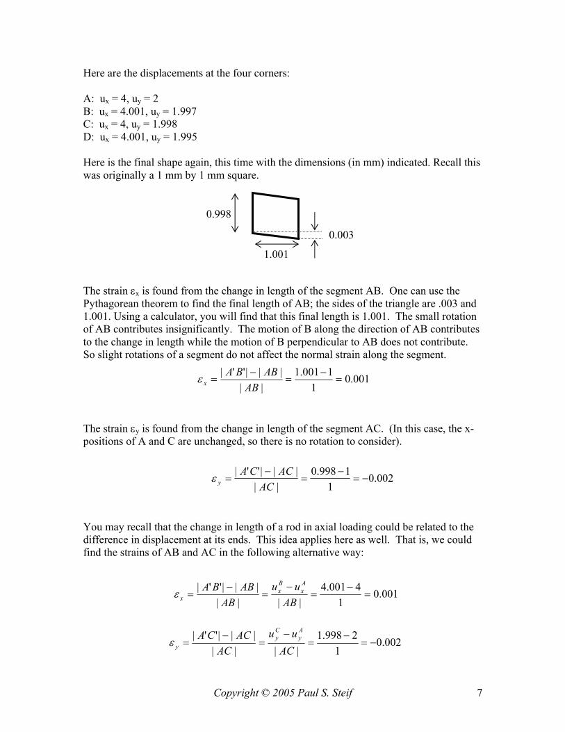
Here are the displacements at the four corners: A: ux = 4, uy = 2 B: ux = 4.001, uy = 1.997 C: ux = 4, uy = 1.998 D: ux = 4.001, uy = 1.995 Here is the final shape again, this time with the dimensions (in mm) indicated. Recall this was originally a 1 mm by 1 mm square. The strain εx is found from the change in length of the segment AB. One can use the Pythagorean theorem to find the final length of AB; the sides of the triangle are .003 and 1.001. Using a calculator, you will find that this final length is 1.001. The small rotation of AB contributes insignificantly. The motion of B along the direction of AB contributes to the change in length while the motion of B perpendicular to AB does not contribute. So slight rotations of a segment do not affect the normal strain along the segment.
The strain εy is found from the change in length of the segment AC. (In this case, the x-positions of A and C are unchanged, so there is no rotation to consider).
You may recall that the change in length of a rod in axial loading could be related to the difference in displacement at its ends. This idea applies here as well. That is, we could find the strains of AB and AC in the following alternative way:
001.01
1001.1||
|||''|=
−=
−=
ABABBA
xε
002.01
1998.0||
|||''|−=
−=
−=
ACACCA
yε
1.001
0.998
0.003
001.01
4001.4||||
|||''|=
−=
−=
−=
ABuu
ABABBA A
xBx
xε
002.01
2998.1||||
|||''|−=
−=
−=
−=
ACuu
ACACCA A
yCy
yε
Copyright © 2005 Paul S. Steif 8
The segment AB rotates clockwise by
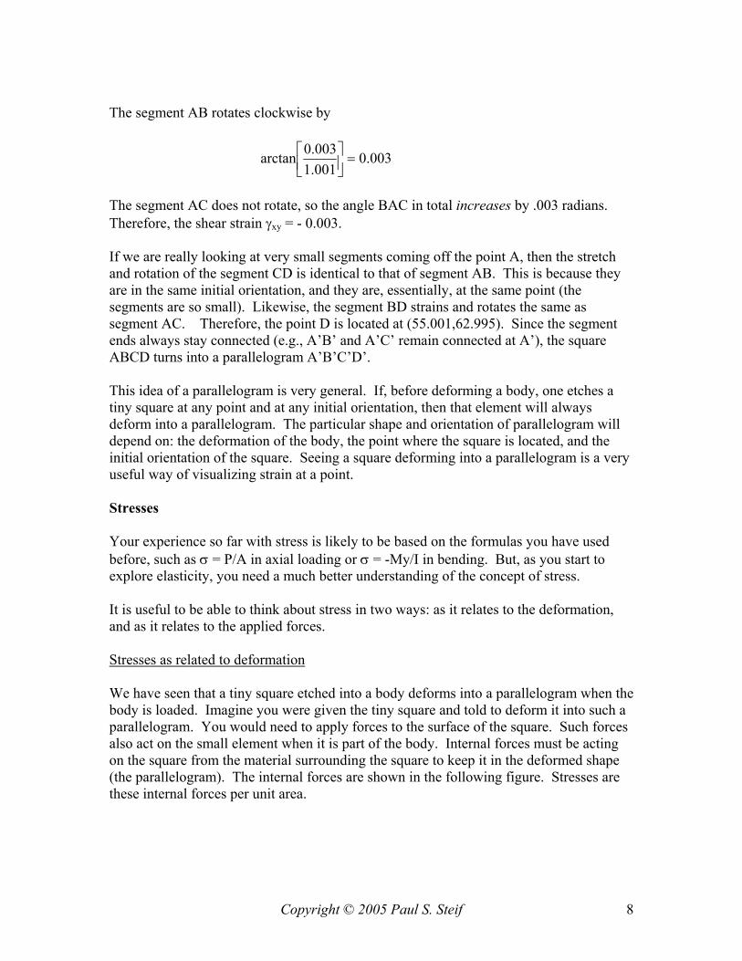
The segment AC does not rotate, so the angle BAC in total increases by .003 radians. Therefore, the shear strain γxy = - 0.003. If we are really looking at very small segments coming off the point A, then the stretch and rotation of the segment CD is identical to that of segment AB. This is because they are in the same initial orientation, and they are, essentially, at the same point (the segments are so small). Likewise, the segment BD strains and rotates the same as segment AC. Therefore, the point D is located at (55.001,62.995). Since the segment ends always stay connected (e.g., A’B’ and A’C’ remain connected at A’), the square ABCD turns into a parallelogram A’B’C’D’. This idea of a parallelogram is very general. If, before deforming a body, one etches a tiny square at any point and at any initial orientation, then that element will always deform into a parallelogram. The particular shape and orientation of parallelogram will depend on: the deformation of the body, the point where the square is located, and the initial orientation of the square. Seeing a square deforming into a parallelogram is a very useful way of visualizing strain at a point. Stresses Your experience so far with stress is likely to be based on the formulas you have used before, such as σ = P/A in axial loading or σ = -My/I in bending. But, as you start to explore elasticity, you need a much better understanding of the concept of stress. It is useful to be able to think about stress in two ways: as it relates to the deformation, and as it relates to the applied forces. Stresses as related to deformation We have seen that a tiny square etched into a body deforms into a parallelogram when the body is loaded. Imagine you were given the tiny square and told to deform it into such a parallelogram. You would need to apply forces to the surface of the square. Such forces also act on the small element when it is part of the body. Internal forces must be acting on the square from the material surrounding the square to keep it in the deformed shape (the parallelogram). The internal forces are shown in the following figure. Stresses are these internal forces per unit area.
003.0001.1003.0arctan =⎥⎦
⎤⎢⎣⎡
Copyright © 2005 Paul S. Steif 9
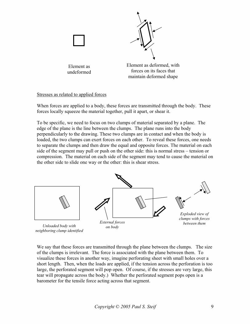
Stresses as related to applied forces When forces are applied to a body, these forces are transmitted through the body. These forces locally squeeze the material together, pull it apart, or shear it. To be specific, we need to focus on two clumps of material separated by a plane. The edge of the plane is the line between the clumps. The plane runs into the body perpendicularly to the drawing. These two clumps are in contact and when the body is loaded, the two clumps can exert forces on each other. To reveal these forces, one needs to separate the clumps and then draw the equal and opposite forces. The material on each side of the segment may pull or push on the other side: this is normal stress – tension or compression. The material on each side of the segment may tend to cause the material on the other side to slide one way or the other: this is shear stress. We say that these forces are transmitted through the plane between the clumps. The size of the clumps is irrelevant. The force is associated with the plane between them. To visualize these forces in another way, imagine perforating sheet with small holes over a short length. Then, when the loads are applied, if the tension across the perforation is too large, the perforated segment will pop open. Of course, if the stresses are very large, this tear will propagate across the body.) Whether the perforated segment pops open is a barometer for the tensile force acting across that segment.
Element as undeformed
Element as deformed, with forces on its faces that
maintain deformed shape
External forces on body
Exploded view of clumps with forces
between them Unloaded body with neighboring clump identified
Copyright © 2005 Paul S. Steif 10
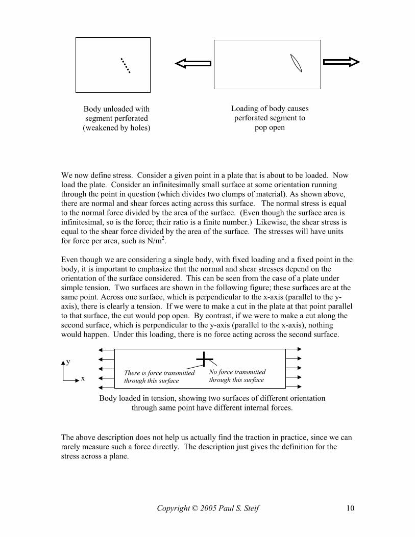
We now define stress. Consider a given point in a plate that is about to be loaded. Now load the plate. Consider an infinitesimally small surface at some orientation running through the point in question (which divides two clumps of material). As shown above, there are normal and shear forces acting across this surface. The normal stress is equal to the normal force divided by the area of the surface. (Even though the surface area is infinitesimal, so is the force; their ratio is a finite number.) Likewise, the shear stress is equal to the shear force divided by the area of the surface. The stresses will have units for force per area, such as N/m2. Even though we are considering a single body, with fixed loading and a fixed point in the body, it is important to emphasize that the normal and shear stresses depend on the orientation of the surface considered. This can be seen from the case of a plate under simple tension. Two surfaces are shown in the following figure; these surfaces are at the same point. Across one surface, which is perpendicular to the x-axis (parallel to the y-axis), there is clearly a tension. If we were to make a cut in the plate at that point parallel to that surface, the cut would pop open. By contrast, if we were to make a cut along the second surface, which is perpendicular to the y-axis (parallel to the x-axis), nothing would happen. Under this loading, there is no force acting across the second surface. The above description does not help us actually find the traction in practice, since we can rarely measure such a force directly. The description just gives the definition for the stress across a plane.
Body unloaded with segment perforated
(weakened by holes)
Loading of body causes perforated segment to
pop open
Body loaded in tension, showing two surfaces of different orientation through same point have different internal forces.
There is force transmitted through this surfacex
y No force transmitted through this surface
Copyright © 2005 Paul S. Steif 11
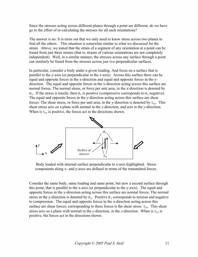
Since the stresses acting across different planes through a point are different, do we have go to the effort of re-calculating the stresses for all such orientations? The answer is no: It is turns out that we only need to know stress across two planes to find all the others. This situation is somewhat similar to what we discussed for the strain. Above, we stated that the strain of a segment of any orientation at a point can be found from just three strains (that is, strains of various orientations are not completely independent). Well, in a similar manner, the stresses across any surface through a point can similarly be found from the stresses across just two perpendicular surfaces. In particular, consider a body under a given loading. And focus on a surface that is parallel to the y-axis (or perpendicular to the x-axis). Across this surface there can be equal and opposite forces in the x-direction and equal and opposite forces in the y-direction. The equal and opposite forces in the x-direction acting across this surface are normal forces. The normal stress, or force per unit area, in the x-direction is denoted by σx. If the stress is tensile, then σx is positive (compressive corresponds to σx negative). The equal and opposite forces in the y-direction acting across this surface are shear forces. The shear stress, or force per unit area, in the y-direction is denoted by τxy. This shear stress acts on a plane with normal in the x-direction, and acts in the y-direction. When is τxy is positive, the forces act in the directions shown. Consider the same body, same loading and same point, but now a second surface through this point, that is parallel to the x-axis (or perpendicular to the y-axis). The equal and opposite forces in the y-direction acting across this surface are normal forces. The normal stress in the y-direction is denoted by σy. Positive σy corresponds to tension and negative to compression. The equal and opposite forces in the x-direction acting across this surface are shear forces; corresponding to these forces is the shear stress τyx. This shear stress acts on a plane with normal in the y-direction, in the x-direction. When is τyx is positive, the forces act in the directions shown.
Body loaded with internal surface perpendicular to x-axis highlighted. Stress components along x- and y-axes are defined in terms of the transmitted forces.
τxy x
y
σx
Surface of interest
Copyright © 2005 Paul S. Steif 12
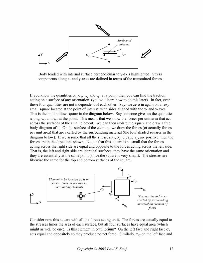
If you know the quantities σx, σy, τxy and τyx at a point, then you can find the traction acting on a surface of any orientation (you will learn how to do this later). In fact, even these four quantities are not independent of each other. Say, we zero in again on a very small square located at the point of interest, with sides aligned with the x- and y-axes. This is the bold hollow square in the diagram below. Say someone gives us the quantities σx, σy, τxy and τyx at the point. This means that we know the forces per unit area that act across the surfaces of the small element. We can then isolate the square and draw a free body diagram of it. On the surface of the element, we draw the forces (or actually forces per unit area) that are exerted by the surrounding material (the four shaded squares in the diagram below). If we assume that all the stresses σx, σy, τxy and τyx are positive, then the forces are in the directions shown. Notice that this square is so small that the forces acting across the right side are equal and opposite to the forces acting across the left side. That is, the left and right side are identical surfaces: they have the same orientation and they are essentially at the same point (since the square is very small). The stresses are likewise the same for the top and bottom surfaces of the square. Consider now this square with all the forces acting on it. The forces are actually equal to the stresses times the area of each surface, but all four surfaces have equal area (which might as well be one). Is this element in equilibrium? On the left face and right face σx acts equal and oppositely so they produce no net force. Similarly, τxy on the left face and
Body loaded with internal surface perpendicular to y-axis highlighted. Stress components along x- and y-axes are defined in terms of the transmitted forces.
τyx
x
y σy
Surface of interest
x
y
σy
τyx
τyx
σy
τxy σx
τxy
σx
Element to be focused on is in center. Stresses are due to
surrounding elements
Stresses due to forces exerted by surrounding material on element of
focus
Copyright © 2005 Paul S. Steif 13
right face is equal and opposite. On the top and bottom, σy and τyx are equal and opposite and so produce no net force. So the sum of forces on this element is zero. Consider, however, the moments. τxy produces a positive moment about the z-axis, and τyx produces a negative moment about the z-axis. These moments only balance if τxy and τyx are equal, which they must be. Therefore, since we have established that τxy = τyx, we only need to be considered about three stresses at the point, which we denote by σx, σy, and τxy. From these one can, with methods to be developed later, determine the stress acting upon any other surface through the point. Again, the stresses σx, σy, and τxy, are really just stresses on two particular planes. Sometimes we can find σx, σy, and τxy from the loads using methods of mechanics of materials. Other times, the loads may be so oriented, or the axes have been so chosen, that the stresses σx, σy, and τxy are not readily found. However, there is nothing special about these three stresses. If we find the stresses acting on two other planes, then we can always find the stresses acting on any additional planes. When we do an elasticity analysis or use the finite element method, we will define the body relative to x- and y-axes. The results of the analysis will be two displacements ux and uy, three strains εx, εy, and γxy, and three stresses σx, σy, and τxy at every point. In the case of the finite element method, you will find these same 8 quantities (ux, uy, εx, εy, γxy, σx, σy, and τxy) at each of the discrete points (nodes) that you or the program defines. This entire discussion presumes a planar (2-D) with forces in the plane. If, instead, the problem is three dimensional, then there are 3 displacements, 6 strains and 6 stresses.
Copyright © 2005 Paul S. Steif 14
2. FORMULATION OF AN ELASTICITY PROBLEM
INTRODUCTION We have already introduced the variables - displacements, strains and stresses – which elasticity theory uses to describe a deforming body. Converting a physical situation in which stresses or deflections are of interest into an elasticity problem involves the same types of steps as for mechanics of materials. One needs to describe: the shape(s) of the deforming body or bodies.
the material properties of the deforming body or bodies.
the loads that are acting on the bodies and/or the constraints on the motion of the
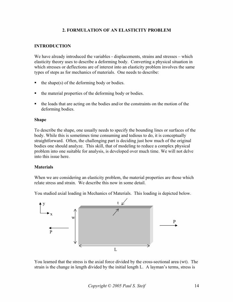
deforming bodies. Shape To describe the shape, one usually needs to specify the bounding lines or surfaces of the body. While this is sometimes time consuming and tedious to do, it is conceptually straightforward. Often, the challenging part is deciding just how much of the original bodies one should analyze. This skill, that of modeling to reduce a complex physical problem into one suitable for analysis, is developed over much time. We will not delve into this issue here. Materials When we are considering an elasticity problem, the material properties are those which relate stress and strain. We describe this now in some detail. You studied axial loading in Mechanics of Materials. This loading is depicted below. You learned that the stress is the axial force divided by the cross-sectional area (wt). The strain is the change in length divided by the initial length L. A layman’s terms, stress is
L
w P
P
x
y t
Copyright © 2005 Paul S. Steif 15
how hard you pull on something and strain is how much it stretches. The intrinsic stiffness of the material controls how hard you must pull on something to get it to stretch a given amount. The intrinsic stiffness of the material is captured by the elastic modulus or Young’s modulus E. E is dependent on the material; materials such as steel, polyethylene, and natural rubber all have very different elastic moduli. However, the elastic modulus is independent of the size of the material or the forces acting upon it. In studying mechanics of materials, you probably only considered stress acting in one direction (say, uniaxial tension). The axial and the transverse strain were related to that stress through the Young’s modulus E, and the Poisson ratio ν. Here we present the relation between stress and strain assuming normal stresses acts in both the x- and y-directions.
EEyx
x
σν
σε −=
EExy
yσ
νσ
ε −=
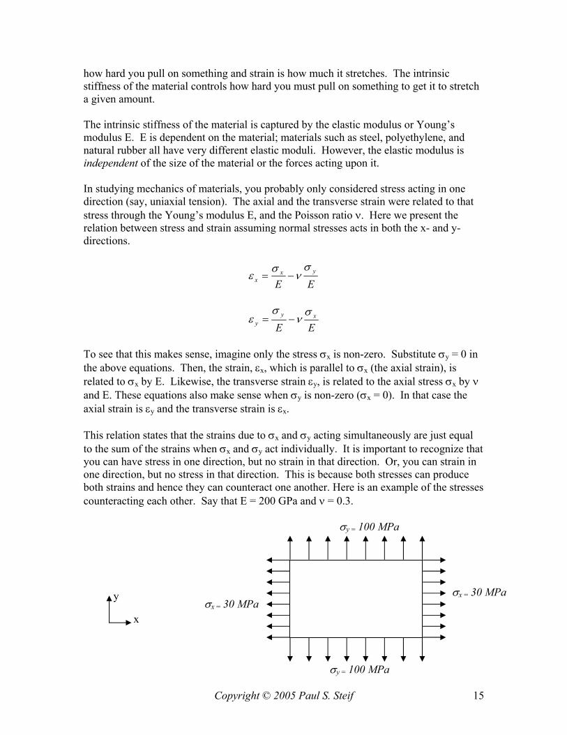
To see that this makes sense, imagine only the stress σx is non-zero. Substitute σy = 0 in the above equations. Then, the strain, εx, which is parallel to σx (the axial strain), is related to σx by E. Likewise, the transverse strain εy, is related to the axial stress σx by ν and E. These equations also make sense when σy is non-zero (σx = 0). In that case the axial strain is εy and the transverse strain is εx. This relation states that the strains due to σx and σy acting simultaneously are just equal to the sum of the strains when σx and σy act individually. It is important to recognize that you can have stress in one direction, but no strain in that direction. Or, you can strain in one direction, but no stress in that direction. This is because both stresses can produce both strains and hence they can counteract one another. Here is an example of the stresses counteracting each other. Say that E = 200 GPa and ν = 0.3.
x
y
σy = 100 MPa
σx = 30 MPa σx = 30 MPa
σy = 100 MPa
Copyright © 2005 Paul S. Steif 16
In this case, the strains are
01020010100)3.0(
102001030
9
6
9
6
=−=−=xx
xx
EEyx
x
σν
σε
000455.010200
1030)3.0(1020010100
9
6
9
6
=−=−=x
xxx
EExy
yσ
νσ
ε
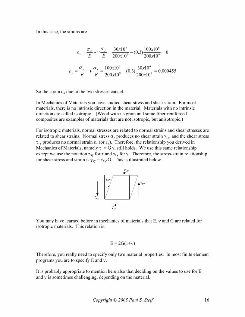
So the strain εx due to the two stresses cancel. In Mechanics of Materials you have studied shear stress and shear strain. For most materials, there is no intrinsic direction in the material. Materials with no intrinsic direction are called isotropic. (Wood with its grain and some fiber-reinforced composites are examples of materials that are not isotropic, but anisotropic.) For isotropic materials, normal stresses are related to normal strains and shear stresses are related to shear strains. Normal stress σx produces no shear strain γxy, and the shear stress τxy produces no normal strain εx (or εy). Therefore, the relationship you derived in Mechanics of Materials, namely τ = G γ, still holds. We use this same relationship except we use the notation τxy for τ and γxy for γ. Therefore, the stress-strain relationship for shear stress and strain is γxy = τxy/G. This is illustrated below.
You may have learned before in mechanics of materials that E, ν and G are related for isotropic materials. This relation is:
E = 2G(1+ν) Therefore, you really need to specify only two material properties. In most finite element programs you are to specify E and ν. It is probably appropriate to mention here also that deciding on the values to use for E and ν is sometimes challenging, depending on the material.
γxy
τyx
τyx
τxy
τxy
Copyright © 2005 Paul S. Steif 17
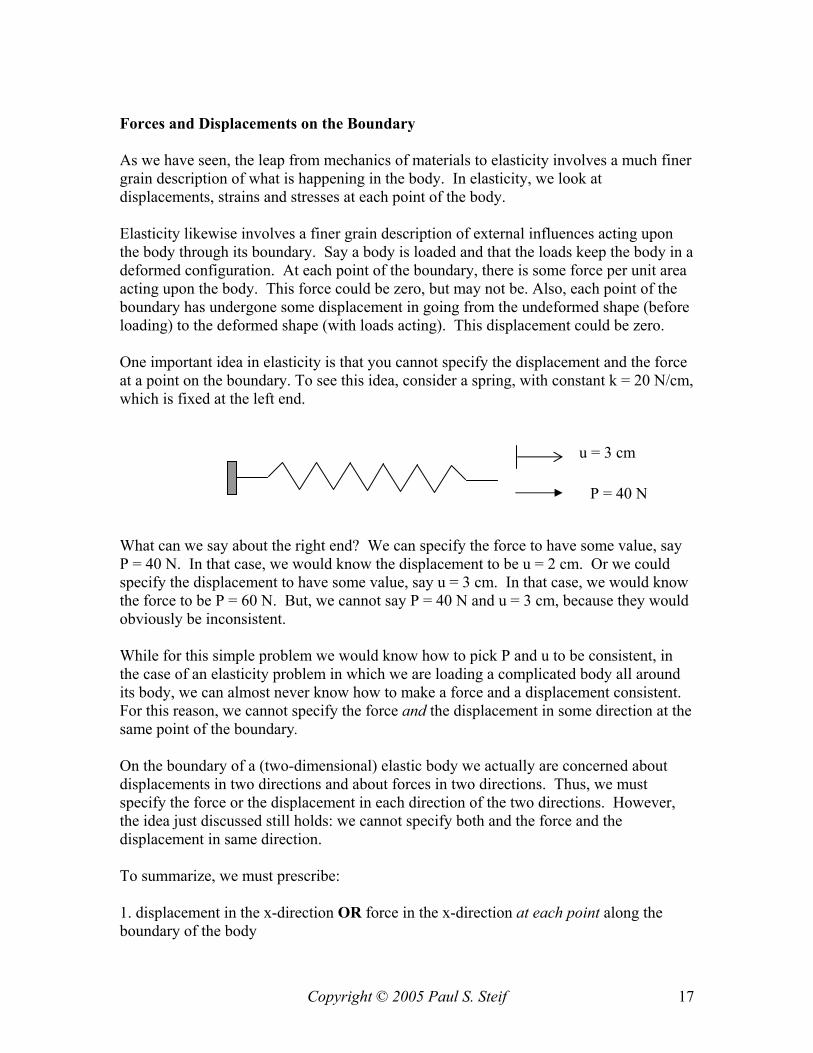
Forces and Displacements on the Boundary As we have seen, the leap from mechanics of materials to elasticity involves a much finer grain description of what is happening in the body. In elasticity, we look at displacements, strains and stresses at each point of the body. Elasticity likewise involves a finer grain description of external influences acting upon the body through its boundary. Say a body is loaded and that the loads keep the body in a deformed configuration. At each point of the boundary, there is some force per unit area acting upon the body. This force could be zero, but may not be. Also, each point of the boundary has undergone some displacement in going from the undeformed shape (before loading) to the deformed shape (with loads acting). This displacement could be zero. One important idea in elasticity is that you cannot specify the displacement and the force at a point on the boundary. To see this idea, consider a spring, with constant k = 20 N/cm, which is fixed at the left end. What can we say about the right end? We can specify the force to have some value, say P = 40 N. In that case, we would know the displacement to be u = 2 cm. Or we could specify the displacement to have some value, say u = 3 cm. In that case, we would know the force to be P = 60 N. But, we cannot say P = 40 N and u = 3 cm, because they would obviously be inconsistent. While for this simple problem we would know how to pick P and u to be consistent, in the case of an elasticity problem in which we are loading a complicated body all around its body, we can almost never know how to make a force and a displacement consistent. For this reason, we cannot specify the force and the displacement in some direction at the same point of the boundary. On the boundary of a (two-dimensional) elastic body we actually are concerned about displacements in two directions and about forces in two directions. Thus, we must specify the force or the displacement in each direction of the two directions. However, the idea just discussed still holds: we cannot specify both and the force and the displacement in same direction. To summarize, we must prescribe: 1. displacement in the x-direction OR force in the x-direction at each point along the boundary of the body
P = 40 N
u = 3 cm
Copyright © 2005 Paul S. Steif 18
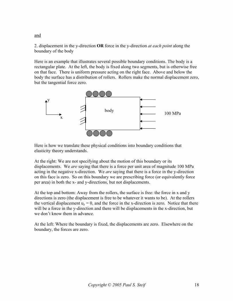
and 2. displacement in the y-direction OR force in the y-direction at each point along the boundary of the body Here is an example that illustrates several possible boundary conditions. The body is a rectangular plate. At the left, the body is fixed along two segments, but is otherwise free on that face. There is uniform pressure acting on the right face. Above and below the body the surface has a distribution of rollers. Rollers make the normal displacement zero, but the tangential force zero. Here is how we translate these physical conditions into boundary conditions that elasticity theory understands. At the right: We are not specifying about the motion of this boundary or its displacements. We are saying that there is a force per unit area of magnitude 100 MPa acting in the negative x-direction. We are saying that there is a force in the y-direction on this face is zero. So on this boundary we are prescribing force (or equivalently force per area) in both the x- and y-directions, but not displacements. At the top and bottom: Away from the rollers, the surface is free: the force in x and y directions is zero (the displacement is free to be whatever it wants to be). At the rollers the vertical displacement uy = 0, and the force in the x-direction is zero. Notice that there will be a force in the y-direction and there will be displacements in the x-direction, but we don’t know them in advance. At the left: Where the boundary is fixed, the displacements are zero. Elsewhere on the boundary, the forces are zero.
body
y
x 100 MPa
Copyright © 2005 Paul S. Steif 19
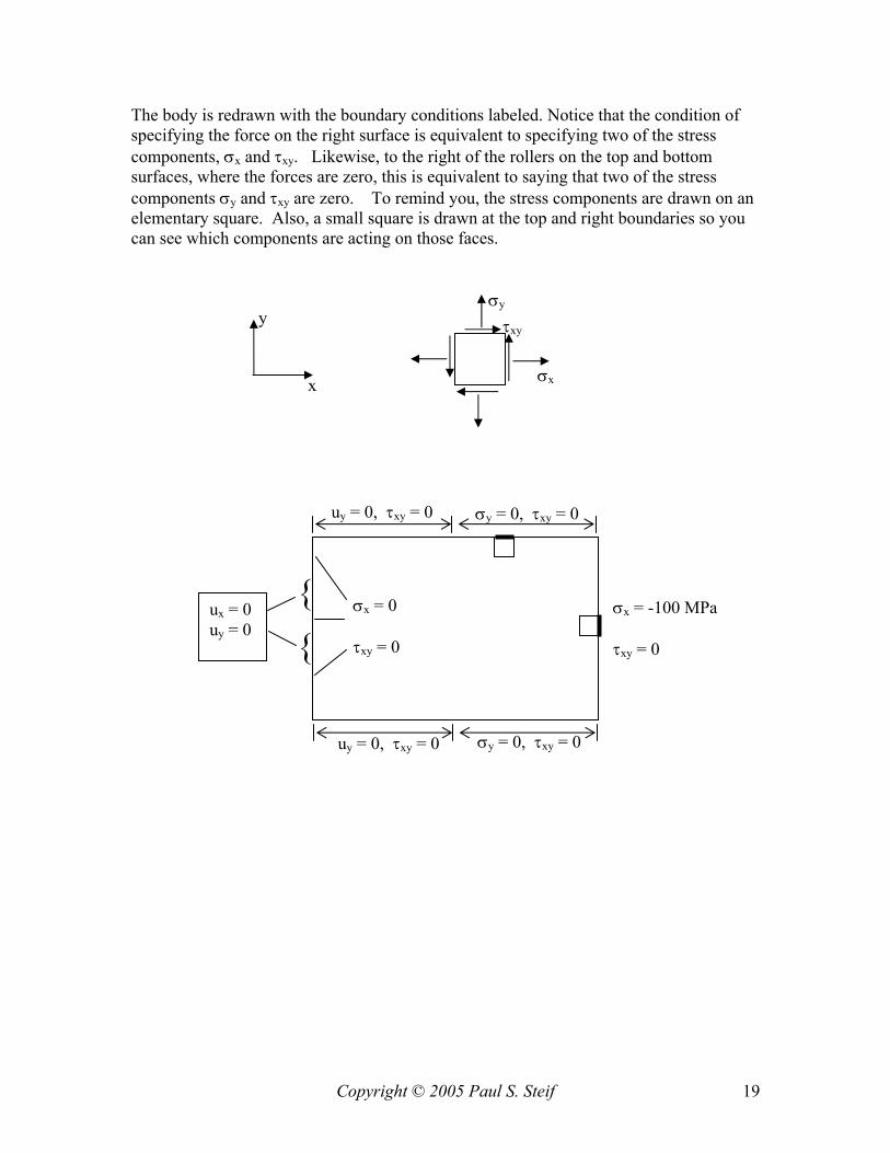
The body is redrawn with the boundary conditions labeled. Notice that the condition of specifying the force on the right surface is equivalent to specifying two of the stress components, σx and τxy. Likewise, to the right of the rollers on the top and bottom surfaces, where the forces are zero, this is equivalent to saying that two of the stress components σy and τxy are zero. To remind you, the stress components are drawn on an elementary square. Also, a small square is drawn at the top and right boundaries so you can see which components are acting on those faces.
y
x σx
σy τxy
σx = -100 MPa τxy = 0
{ {
ux = 0 uy = 0
σx = 0 τxy = 0
σy = 0, τxy = 0 uy = 0, τxy = 0
σy = 0, τxy = 0 uy = 0, τxy = 0
Copyright © 2005 Paul S. Steif 20
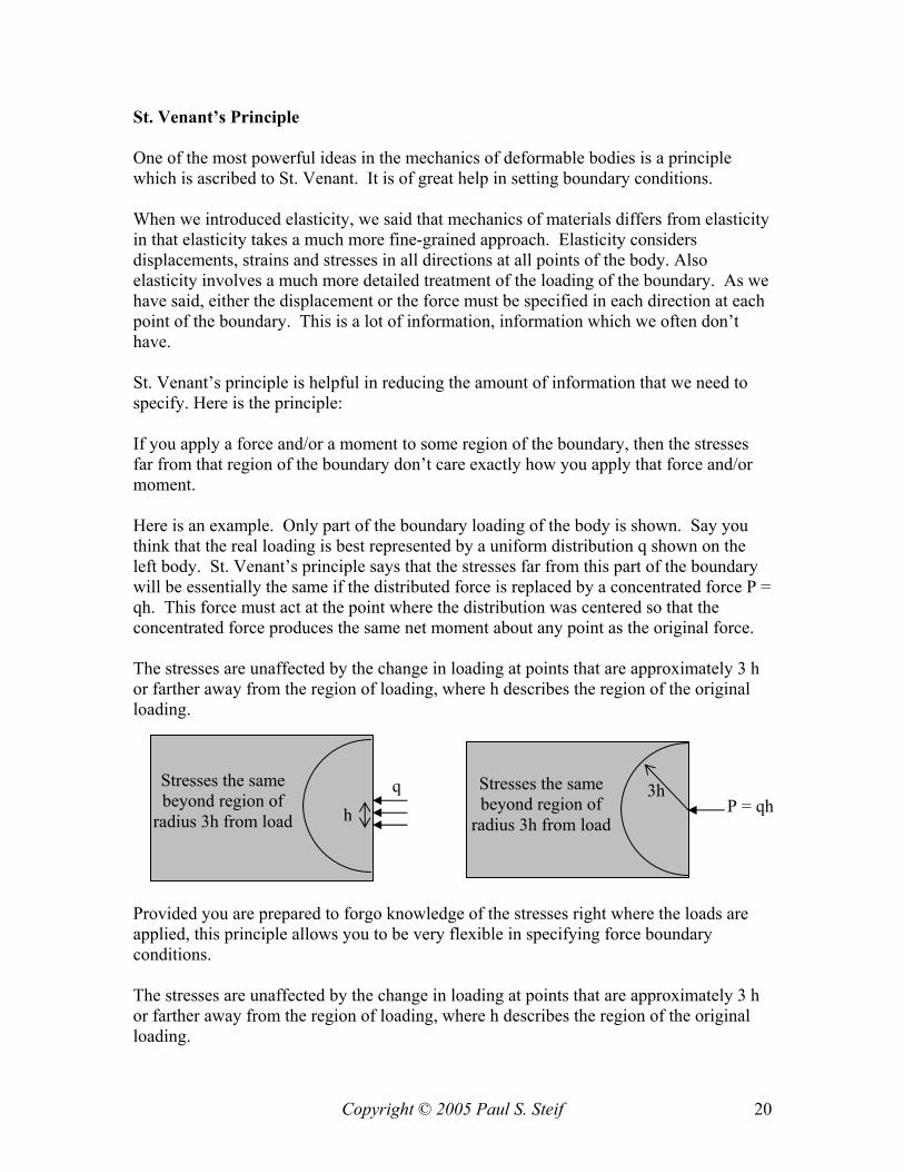
St. Venant’s Principle One of the most powerful ideas in the mechanics of deformable bodies is a principle which is ascribed to St. Venant. It is of great help in setting boundary conditions. When we introduced elasticity, we said that mechanics of materials differs from elasticity in that elasticity takes a much more fine-grained approach. Elasticity considers displacements, strains and stresses in all directions at all points of the body. Also elasticity involves a much more detailed treatment of the loading of the boundary. As we have said, either the displacement or the force must be specified in each direction at each point of the boundary. This is a lot of information, information which we often don’t have. St. Venant’s principle is helpful in reducing the amount of information that we need to specify. Here is the principle: If you apply a force and/or a moment to some region of the boundary, then the stresses far from that region of the boundary don’t care exactly how you apply that force and/or moment. Here is an example. Only part of the boundary loading of the body is shown. Say you think that the real loading is best represented by a uniform distribution q shown on the left body. St. Venant’s principle says that the stresses far from this part of the boundary will be essentially the same if the distributed force is replaced by a concentrated force P = qh. This force must act at the point where the distribution was centered so that the concentrated force produces the same net moment about any point as the original force. The stresses are unaffected by the change in loading at points that are approximately 3 h or farther away from the region of loading, where h describes the region of the original loading. Provided you are prepared to forgo knowledge of the stresses right where the loads are applied, this principle allows you to be very flexible in specifying force boundary conditions. The stresses are unaffected by the change in loading at points that are approximately 3 h or farther away from the region of loading, where h describes the region of the original loading.
h 3h
P = qh Stresses the same beyond region of
radius 3h from load
q Stresses the same beyond region of
radius 3h from load

Copyright © 2005 Paul S. Steif 21
EQUATIONS OF EQUILIBRIUM AND COMPATIBILITY When you solved problems using mechanics of materials you used three principles. One principle was the material law or stress-strain relation. For the case of elasticity, we have discussed that above. The second principle is mechanical equilibrium, that is the sum of forces and moments both equal zero. The third principle is geometric compatibility, that is the geometric relations between the motions and the strains. Elasticity also uses these principles, FEA which is based on elasticity uses these principles. Unless you solve equations of elasticity directly, you probably don’t need to know how equilibrium and geometric compatibility are implemented in elasticity. For completeness though, we present these equations below: Equilibrium When the stresses vary from point to point, they are in equilibrium with each other and with any forces applied on the boundary. For three dimensional stress state, this results in 3 partial differential equations involving the 6 components of stress. When there is a planar state of stress (only σx, σy, and τxy), then there are only two such equations and they are as follows:
Geometric Compatibility The strains are related to variations in the displacements. These relations generalize the basic relation from axial loading ε = δ/L and a similar one for shear strain. For displacements in three-dimensions, this results in 6 partial differential equations involving the strains and the displacements. For a planar deformation, there are 3 relations between strain and displacement
In total, for three-dimensional problems there are 15 equations for the 6 stresses, 6 strains and 3 displacements. For a plane stress problem there are 8 equations for the 3 stresses (σx, σy, and τxy), 3 strains (εx, εy, and γxy) and 2 displacements (ux and uy). In addition, there are boundary conditions, which we have described above for the case of plane stress problems.
00 =∂
∂+
∂∂
=∑ yximpliesF xyx
x
τσ
00 =∂
∂+
∂
∂=∑ yx
impliesF yxyy
στ
xux
x ∂∂
=εy
u yy ∂
∂=ε x
uy
u yxxy ∂
∂+
∂∂
=γ

Copyright © 2005 Paul S. Steif 22
3. FINITE ELEMENT METHOD The equations of elasticity are partial differential equations that are to be satisfied at every point of the body. Furthermore the displacements or stresses must satisfy specified values on the boundary. Because the equations of elasticity are so difficult to solve, the finite element method has been developed to solve these equations on the computer. The results of this method are stresses or displacements that are approximate relative to what elasticity would give. Very briefly, the finite element method solves these equations by breaking up the body into small, but finite regions. The method presumes that the key quantities, displacements, strains and stresses, have a simple spatial distribution within each element. For example, the stresses might vary linearly with position in each element. These key quantities are then chosen to satisfy the equations of elasticity approximately. Breaking up the body appropriately into a mesh of elements is important to getting good estimates of the stresses. Most finite element programs have a variety of methods to help you do meshing. In the end, though, the mesh will consist of a set of node points distributed around the body. The node points will be connected by lines and the lines form the boundaries of the elements. This is illustrated in the figure below.
Below are the major steps in a finite element analysis. Define the Region This is describing the shape and position of the body. Define Material Properties Usually this includes the elastic modulus (E) and the Poisson ratio (ν), although other parameters could be of interest (such as thermal expansion coefficient). Define Type(s) of Element One must choose the type of elements that are to be used, which depends on the type of analysis. One type of element differs from another insofar as the variables that it deals
nodes elements
Boundary nodes
Copyright © 2005 Paul S. Steif 23
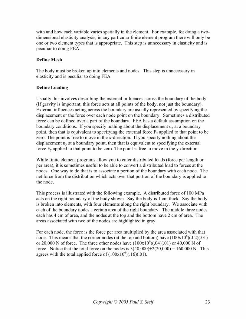
with and how each variable varies spatially in the element. For example, for doing a two-dimensional elasticity analysis, in any particular finite element program there will only be one or two element types that is appropriate. This step is unnecessary in elasticity and is peculiar to doing FEA. Define Mesh The body must be broken up into elements and nodes. This step is unnecessary in elasticity and is peculiar to doing FEA. Define Loading Usually this involves describing the external influences across the boundary of the body (If gravity is important, this force acts at all points of the body, not just the boundary). External influences acting across the boundary are usually represented by specifying the displacement or the force over each node point on the boundary. Sometimes a distributed force can be defined over a part of the boundary. FEA has a default assumption on the boundary conditions. If you specify nothing about the displacement ux at a boundary point, then that is equivalent to specifying the external force Fx applied to that point to be zero. The point is free to move in the x-direction. If you specify nothing about the displacement uy at a boundary point, then that is equivalent to specifying the external force Fy applied to that point to be zero. The point is free to move in the y-direction. While finite element programs allow you to enter distributed loads (force per length or per area), it is sometimes useful to be able to convert a distributed load to forces at the nodes. One way to do that is to associate a portion of the boundary with each node. The net force from the distribution which acts over that portion of the boundary is applied to the node. This process is illustrated with the following example. A distributed force of 100 MPa acts on the right boundary of the body shown. Say the body is 1 cm thick. Say the body is broken into elements, with four elements along the right boundary. We associate with each of the boundary nodes a certain area of the right boundary. The middle three nodes each has 4 cm of area, and the nodes at the top and the bottom have 2 cm of area. The areas associated with two of the nodes are highlighted in gray. For each node, the force is the force per area multiplied by the area associated with that node. This means that the corner nodes (at the top and bottom) have (100x106)(.02)(.01) or 20,000 N of force. The three other nodes have (100x106)(.04)(.01) or 40,000 N of force. Notice that the total force on the nodes is 3(40,000)+2(20,000) = 160,000 N. This agrees with the total applied force of (100x106)(.16)(.01).
Copyright © 2005 Paul S. Steif 24
Request Solution When doing FEA, one usually just pushes a button which solves the problem that has been specified. This solves the equations of elasticity approximately. Inspect Results When doing FEA, one can view the results in a variety ways. More on Meshing As mentioned above, the finite element method solves the equations of elasticity approximately. How good is that approximation? It depends on the elasticity problem, and it depends on the mesh. There are some elasticity problems which can never be solved with FEA; this is discussed later in the chapter on Stress Concentrations and Singularities. For problems with no singularities, FEA is capable of offering estimates of stress that are comparable to those given by elasticity. As we said above, FEA works by assuming an approximate variation of stress over each element, for example a linear variation. FEA gives the most accurate answers if the actual stress varies over the element in the same way as assumed by the element. So if the stress actually varies linearly with position (as it does in pure bending), then FEA with elements assuming a linear variation in stress will approximate the actual stress field exactly. Under most loadings, the stresses will vary in a more complex way. So how can FEA approximate this accurately? Consider a general function y(x) that is continuous and smooth. If you look at y(x) over a small enough region, y(x) can be approximated by a linear function (using the derivative). This means that if the elements are taken to be small enough, so the stresses
(100x106)(.02)(.01) = 20,000 N
16 cm 100 MPa
(100x106)(.04)(.01) = 40,000 N
4 cm
Copyright © 2005 Paul S. Steif 25
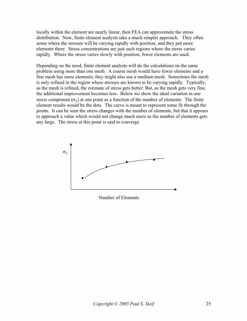
locally within the element are nearly linear, then FEA can approximate the stress distribution. Now, finite element analysts take a much simpler approach. They often sense where the stresses will be varying rapidly with position, and they put more elements there. Stress concentrations are just such regions where the stress varies rapidly. Where the stress varies slowly with position, fewer elements are used. Depending on the need, finite element analysts will do the calculations on the same problem using more than one mesh. A coarse mesh would have fewer elements and a fine mesh has more elements; they might also use a medium mesh. Sometimes the mesh is only refined in the region where stresses are known to be varying rapidly. Typically, as the mesh is refined, the estimate of stress gets better. But, as the mesh gets very fine, the additional improvement becomes less. Below we show the ideal variation in one stress component (σx) at one point as a function of the number of elements. The finite element results would be the dots. The curve is meant to represent some fit through the points. It can be seen the stress changes with the number of elements, but that it appears to approach a value which would not change much more as the number of elements gets any large. The stress at this point is said to converge.
σx
Number of Elements
Copyright © 2005 Paul S. Steif 26
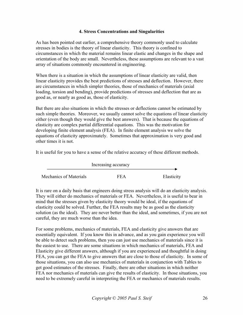
4. Stress Concentrations and Singularities As has been pointed out earlier, a comprehensive theory commonly used to calculate stresses in bodies is the theory of linear elasticity. This theory is confined to circumstances in which the material remains linear elastic and changes in the shape and orientation of the body are small. Nevertheless, these assumptions are relevant to a vast array of situations commonly encountered in engineering. When there is a situation in which the assumptions of linear elasticity are valid, then linear elasticity provides the best predictions of stresses and deflection. However, there are circumstances in which simpler theories, those of mechanics of materials (axial loading, torsion and bending), provide predictions of stresses and deflection that are as good as, or nearly as good as, those of elasticity. But there are also situations in which the stresses or deflections cannot be estimated by such simple theories. Moreover, we usually cannot solve the equations of linear elasticity either (even though they would give the best answers). That is because the equations of elasticity are complex partial differential equations. This was the motivation for developing finite element analysis (FEA). In finite element analysis we solve the equations of elasticity approximately. Sometimes that approximation is very good and other times it is not. It is useful for you to have a sense of the relative accuracy of these different methods. It is rare on a daily basis that engineers doing stress analysis will do an elasticity analysis. They will either do mechanics of materials or FEA. Nevertheless, it is useful to bear in mind that the stresses given by elasticity theory would be ideal, if the equations of elasticity could be solved. Further, the FEA results may be as good as the elasticity solution (as the ideal). They are never better than the ideal, and sometimes, if you are not careful, they are much worse than the idea. For some problems, mechanics of materials, FEA and elasticity give answers that are essentially equivalent. If you know this in advance, and as you gain experience you will be able to detect such problems, then you can just use mechanics of materials since it is the easiest to use. There are some situations in which mechanics of materials, FEA and Elasticity give different answers, although if you are experienced and thoughtful in doing FEA, you can get the FEA to give answers that are close to those of elasticity. In some of those situations, you can also use mechanics of materials in conjunction with Tables to get good estimates of the stresses. Finally, there are other situations in which neither FEA nor mechanics of materials can give the results of elasticity. In those situations, you need to be extremely careful in interpreting the FEA or mechanics of materials results.
Increasing accuracy
Mechanics of Materials FEA Elasticity
Copyright © 2005 Paul S. Steif 27
In the next Chapter, we outline situations in which mechanics of materials leads to reasonably accurate predictions of stress and deflection. (We also show there how mechanics of materials can be used to give very rough estimates of these quantities, just to make sure you have not made some gross error in FEA.) Here we consider situations in which FEA or elasticity is necessary to arrive at estimates of stress. Typically, these involve situations in which the stresses are locally concentrated, beyond the normal variations of stress found in mechanics materials. It will be important to distinguish between situations in which FEA, if used appropriately, can give good estimates of stresses, and those situations in FEA cannot. FEA is a very powerful tool if used properly, but it can be misleading or dangerous in the hands of someone who is not fully prepared to use it. In considering situations in which stresses are concentrated, we distinguish between two types of situations:
• Stress Concentrations and Singularities associated with Boundary Shape
These concentrations are real and of genuine concern in design
• Stress Concentrations and Singularities induced by loading or supports
These are due to the idealized, unrealistic ways in which loads or supports are commonly applied in FEA
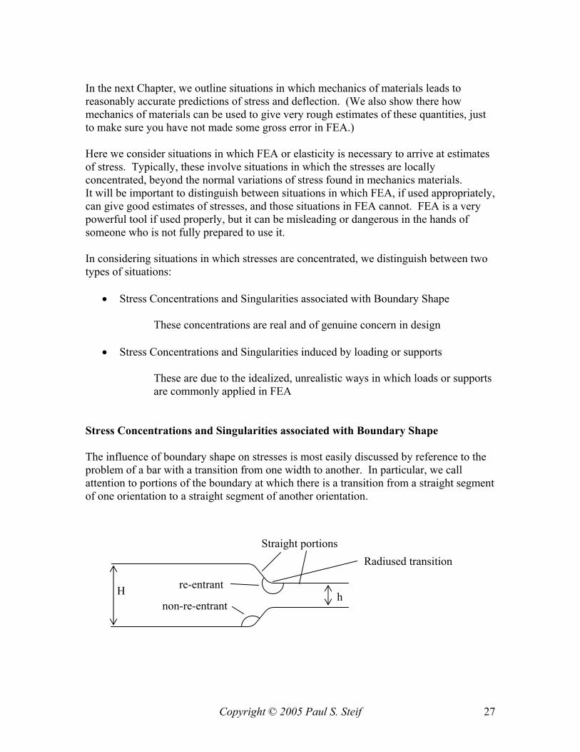
Stress Concentrations and Singularities associated with Boundary Shape The influence of boundary shape on stresses is most easily discussed by reference to the problem of a bar with a transition from one width to another. In particular, we call attention to portions of the boundary at which there is a transition from a straight segment of one orientation to a straight segment of another orientation.
H h
Straight portions Radiused transition
re-entrant
non-re-entrant
Copyright © 2005 Paul S. Steif 28
Near the transition, or corner, the body occupies a sector with some angle. The sectors are labeled in the figure. When the sector occupies angle which is greater than 180°, the transition is considered a re-entrant corner. When the sector occupies angle which is less than 180°, the transition is considered a non-re-entrant corner. At a re-entrant corner (angle > 180°), the stresses will be greater than if this feature were absent. In this situation the stress would be greater than the simple axial loading prediction of P/ht (where t is the thickness into the paper). By contrast, for non-re-entrant corners, the stresses are low (even lower than P/Ht here). The ratio of the actual maximum stress to the stress P/A is termed the stress concentration. The stress concentration depends on the radius of the transition. The smaller the radius, the more rapid the transition from one boundary to another, the higher is the stress concentrations. It is widely known in mechanical design that one needs to consider reducing stress concentrations, particularly when the loads are alternating, that is, when fatigue is of concern. Very sharp corners are to be avoided. One can talk theoretically about the radius of the transition going to zero, that is, an immediate transition from one orientation to the other or a truly sharp corner. In this case the theory of elasticity says that the stresses are infinite. Of course, no corner is truly sharp; moreover, the assumptions of linear elasticity break down in such regions. Thus, the predictions of infinite stresses are not really correct. Nevertheless, there are advanced theories (fracture mechanics) that enable one to interpret the infinite stress in a meaningful way. Consider now the use of FEA to analyze such a transition. When the radius is known, and one wants an accurate estimate of the stresses, then the right radius has to be included in the finite element model. Also, a sufficient number of mesh points must be placed around the transition. On the other hand, it is sometimes very convenient to ignore the radius and set up a finite element model with the two boundaries meeting at a point. The FEA results near the transition will be completely unreliable. Elasticity theory, which FEA is trying to approximate, says that the stresses are infinite at the corner. But, FEA always gives finite stresses. Rather than converge, the FEA stresses at the corner will simply continue to increase as more mesh points are placed near the transition. Therefore, one has to recognize such situations in which the FEA results cannot offer good estimates of stresses. Concentration/singularity due to Loading We have introduced St. Venant’s principle earlier in the chapter on formulation of elasticity problems. It states that the stresses far from region of load application are dependent only on the load, not on the precise way in which the loads are applied. However, the stresses in the immediate vicinity of load application are dependent on how the loads are applied. If the force is applied over a smaller area then the stresses locally
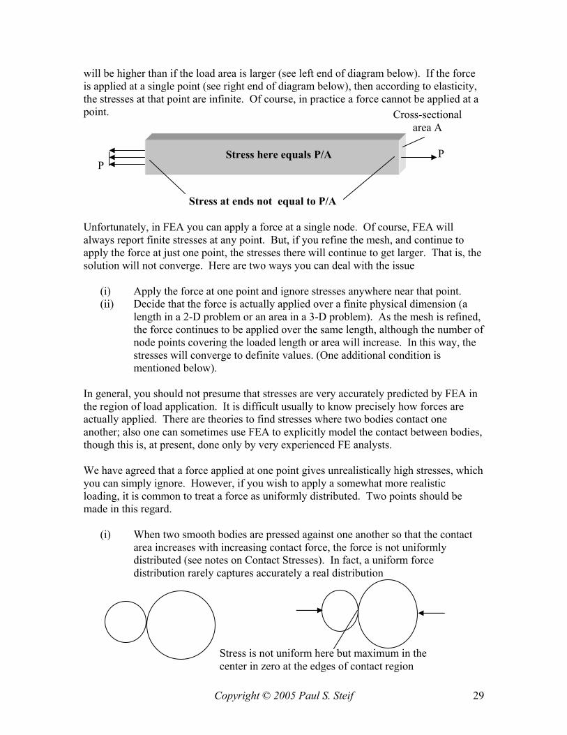
Copyright © 2005 Paul S. Steif 29
will be higher than if the load area is larger (see left end of diagram below). If the force is applied at a single point (see right end of diagram below), then according to elasticity, the stresses at that point are infinite. Of course, in practice a force cannot be applied at a point. Unfortunately, in FEA you can apply a force at a single node. Of course, FEA will always report finite stresses at any point. But, if you refine the mesh, and continue to apply the force at just one point, the stresses there will continue to get larger. That is, the solution will not converge. Here are two ways you can deal with the issue
(i) Apply the force at one point and ignore stresses anywhere near that point. (ii) Decide that the force is actually applied over a finite physical dimension (a
length in a 2-D problem or an area in a 3-D problem). As the mesh is refined, the force continues to be applied over the same length, although the number of node points covering the loaded length or area will increase. In this way, the stresses will converge to definite values. (One additional condition is mentioned below).
In general, you should not presume that stresses are very accurately predicted by FEA in the region of load application. It is difficult usually to know precisely how forces are actually applied. There are theories to find stresses where two bodies contact one another; also one can sometimes use FEA to explicitly model the contact between bodies, though this is, at present, done only by very experienced FE analysts. We have agreed that a force applied at one point gives unrealistically high stresses, which you can simply ignore. However, if you wish to apply a somewhat more realistic loading, it is common to treat a force as uniformly distributed. Two points should be made in this regard.
(i) When two smooth bodies are pressed against one another so that the contact area increases with increasing contact force, the force is not uniformly distributed (see notes on Contact Stresses). In fact, a uniform force distribution rarely captures accurately a real distribution
P P
Stress here equals P/A
Cross-sectional area A
Stress at ends not equal to P/A
Stress is not uniform here but maximum in the center in zero at the edges of contact region
Copyright © 2005 Paul S. Steif 30
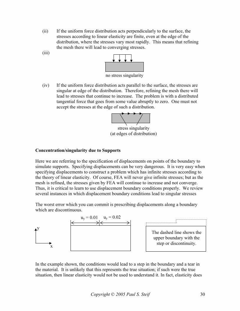
(ii) If the uniform force distribution acts perpendicularly to the surface, the stresses according to linear elasticity are finite, even at the edge of the distribution, where the stresses vary most rapidly. This means that refining the mesh there will lead to converging stresses.
(iii)
(iv) If the uniform force distribution acts parallel to the surface, the stresses are
singular at edge of the distribution. Therefore, refining the mesh there will lead to stresses that continue to increase. The problem is with a distributed tangential force that goes from some value abruptly to zero. One must not accept the stresses at the edge of such a distribution.
Concentration/singularity due to Supports Here we are referring to the specification of displacements on points of the boundary to simulate supports. Specifying displacements can be very dangerous. It is very easy when specifying displacements to construct a problem which has infinite stresses according to the theory of linear elasticity. Of course, FEA will never give infinite stresses; but as the mesh is refined, the stresses given by FEA will continue to increase and not converge. Thus, it is critical to learn to use displacement boundary conditions properly. We review several instances in which displacement boundary conditions lead to singular stresses The worst error which you can commit is prescribing displacements along a boundary which are discontinuous. In the example shown, the conditions would lead to a step in the boundary and a tear in the material. It is unlikely that this represents the true situation; if such were the true situation, then linear elasticity would not be used to understand it. In fact, elasticity does
uy = 0.01 uy = 0.02
stress singularity (at edges of distribution)
no stress singularity
y
x
The dashed line shows the upper boundary with the
step or discontinuity.
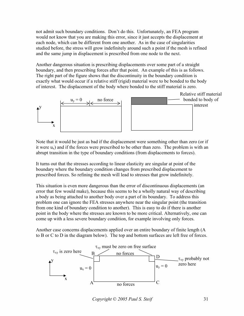
Copyright © 2005 Paul S. Steif 31
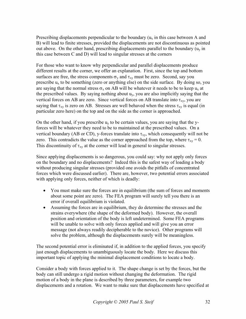
not admit such boundary conditions. Don’t do this. Unfortunately, an FEA program would not know that you are making this error, since it just accepts the displacement at each node, which can be different from one another. As in the case of singularities studied before, the stress will grow indefinitely around such a point if the mesh is refined and the same jump in displacement is prescribed from one node to the next. Another dangerous situation is prescribing displacements over some part of a straight boundary, and then prescribing forces after that point. An example of this is as follows. The right part of the figure shows that the discontinuity in the boundary condition is exactly what would occur if a relative stiff (rigid) material were to be bonded to the body of interest. The displacement of the body where bonded to the stiff material is zero. Note that it would be just as bad if the displacement were something other than zero (or if it were ux) and if the forces were prescribed to be other than zero. The problem is with an abrupt transition in the type of boundary conditions (from displacements to forces). It turns out that the stresses according to linear elasticity are singular at point of the boundary where the boundary condition changes from prescribed displacement to prescribed forces. So refining the mesh will lead to stresses that grow indefinitely. This situation is even more dangerous than the error of discontinuous displacements (an error that few would make), because this seems to be a wholly natural way of describing a body as being attached to another body over a part of its boundary. To address this problem one can ignore the FEA stresses anywhere near the singular point (the transition from one kind of boundary condition to another). This is easy to do if there is another point in the body where the stresses are known to be more critical. Alternatively, one can come up with a less severe boundary condition, for example involving only forces. Another case concerns displacements applied over an entire boundary of finite length (A to B or C to D in the diagram below). The top and bottom surfaces are left free of forces.
uy = 0 no force y
x
Relative stiff material bonded to body of
interest
uy = 0 ux = 0
A
B
C
D
no forces
no forces y
x
τxy must be zero on free surface τxy is zero here
τxy probably not zero here
Copyright © 2005 Paul S. Steif 32
Prescribing displacements perpendicular to the boundary (ux in this case between A and B) will lead to finite stresses, provided the displacements are not discontinuous as pointed out above. On the other hand, prescribing displacements parallel to the boundary (uy in this case between C and D) will lead to singular stresses at the corners For those who want to know why perpendicular and parallel displacements produce different results at the corner, we offer an explanation. First, since the top and bottom surfaces are free, the stress components σy and τxy must be zero. Second, say you prescribe ux to be something (zero or anything else) on the side surface. By doing so, you are saying that the normal stress σx on AB will be whatever it needs to be to keep ux at the prescribed values. By saying nothing about uy, you are also implicitly saying that the vertical forces on AB are zero. Since vertical forces on AB translate into τxy, you are saying that τxy is zero on AB. Stresses are well behaved when the stress τxy is equal (in particular zero here) on the top and on the side as the corner is approached. On the other hand, if you prescribe uy to be certain values, you are saying that the y-forces will be whatever they need to be to maintained at the prescribed values. On a vertical boundary (AB or CD), y-forces translate into τxy, which consequently will not be zero. This contradicts the value as the corner approached from the top, where τxy = 0. This discontinuity of τxy at the corner will lead in general to singular stresses. Since applying displacements is so dangerous, you could say: why not apply only forces on the boundary and no displacements? Indeed this is the safest way of loading a body without producing singular stresses (provided one avoids the pitfalls of concentrated forces which were discussed earlier). There are, however, two potential errors associated with applying only forces, neither of which is deadly:
• You must make sure the forces are in equilibrium (the sum of forces and moments about some point are zero). The FEA program will surely tell you there is an error if overall equilibrium is violated.
• Assuming the forces are in equilibrium, they do determine the stresses and the strains everywhere (the shape of the deformed body). However, the overall position and orientation of the body is left undetermined. Some FEA programs will be unable to solve with only forces applied and will give you an error message (not always readily decipherable to the novice). Other programs will solve the problem, although the displacements surely will be meaningless.
The second potential error is eliminated if, in addition to the applied forces, you specify just enough displacements to unambiguously locate the body. Here we discuss this important topic of applying the minimal displacement conditions to locate a body. Consider a body with forces applied to it. The shape change is set by the forces, but the body can still undergo a rigid motion without changing the deformation. The rigid motion of a body in the plane is described by three parameters, for example two displacements and a rotation. We want to make sure that displacements have specified at
Copyright © 2005 Paul S. Steif 33
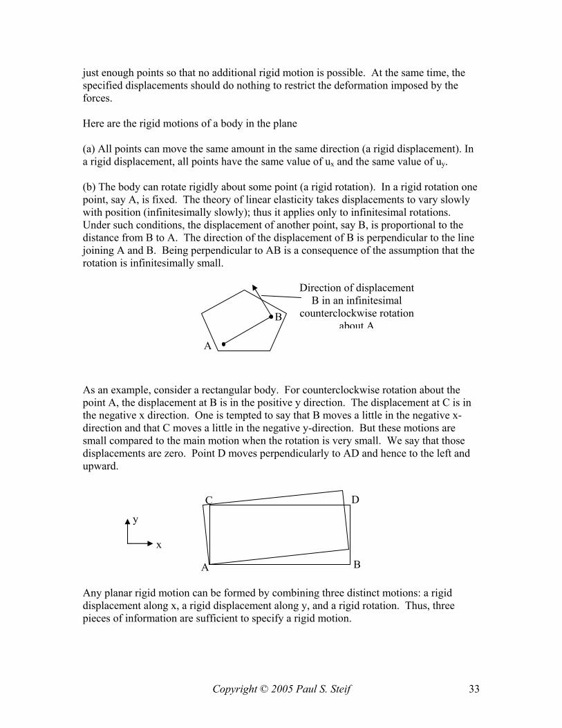
just enough points so that no additional rigid motion is possible. At the same time, the specified displacements should do nothing to restrict the deformation imposed by the forces. Here are the rigid motions of a body in the plane (a) All points can move the same amount in the same direction (a rigid displacement). In a rigid displacement, all points have the same value of ux and the same value of uy. (b) The body can rotate rigidly about some point (a rigid rotation). In a rigid rotation one point, say A, is fixed. The theory of linear elasticity takes displacements to vary slowly with position (infinitesimally slowly); thus it applies only to infinitesimal rotations. Under such conditions, the displacement of another point, say B, is proportional to the distance from B to A. The direction of the displacement of B is perpendicular to the line joining A and B. Being perpendicular to AB is a consequence of the assumption that the rotation is infinitesimally small. As an example, consider a rectangular body. For counterclockwise rotation about the point A, the displacement at B is in the positive y direction. The displacement at C is in the negative x direction. One is tempted to say that B moves a little in the negative x- direction and that C moves a little in the negative y-direction. But these motions are small compared to the main motion when the rotation is very small. We say that those displacements are zero. Point D moves perpendicularly to AD and hence to the left and upward. Any planar rigid motion can be formed by combining three distinct motions: a rigid displacement along x, a rigid displacement along y, and a rigid rotation. Thus, three pieces of information are sufficient to specify a rigid motion.
A
B
Direction of displacement B in an infinitesimal
counterclockwise rotation about A
A B
C D
x
y
Copyright © 2005 Paul S. Steif 34
Consider again the body with the forces applied to it. The shape change is set, but the body can undergo a rigid motion. We now know that the rigid motion can be set if we know three pieces of information regarding the motion of the body. Since one typically cannot specify rotations in elasticity theory, but only displacements, in practice one specifies three displacements. This typically would involve specifying two displacements at one point and one displacement at another point. However are there are pitfalls to avoid:
• The displacements must not restrict the strain of the body (which is dictated by the applied forces and the resulting stress distribution)
• The displacements must not leave open the possibility of an arbitrary rigid motion
of any kind. (This was the whole reason that we took to studying minimal locating displacements in the first place.)
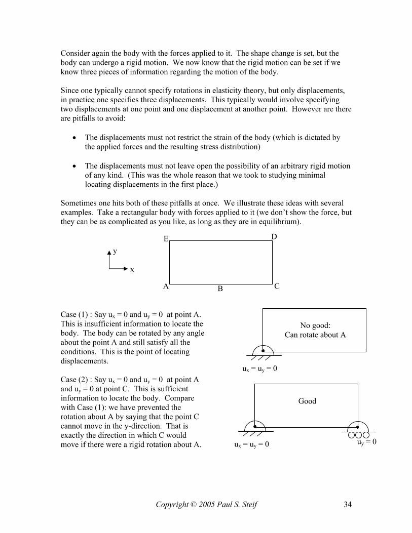
Sometimes one hits both of these pitfalls at once. We illustrate these ideas with several examples. Take a rectangular body with forces applied to it (we don’t show the force, but they can be as complicated as you like, as long as they are in equilibrium). Case (1) : Say ux = 0 and uy = 0 at point A. This is insufficient information to locate the body. The body can be rotated by any angle about the point A and still satisfy all the conditions. This is the point of locating displacements. Case (2) : Say ux = 0 and uy = 0 at point A and uy = 0 at point C. This is sufficient information to locate the body. Compare with Case (1): we have prevented the rotation about A by saying that the point C cannot move in the y-direction. That is exactly the direction in which C would move if there were a rigid rotation about A.
A B C
D
x
y E
No good: Can rotate about A
ux = uy = 0
Good
ux = uy = 0 uy = 0
Copyright © 2005 Paul S. Steif 35
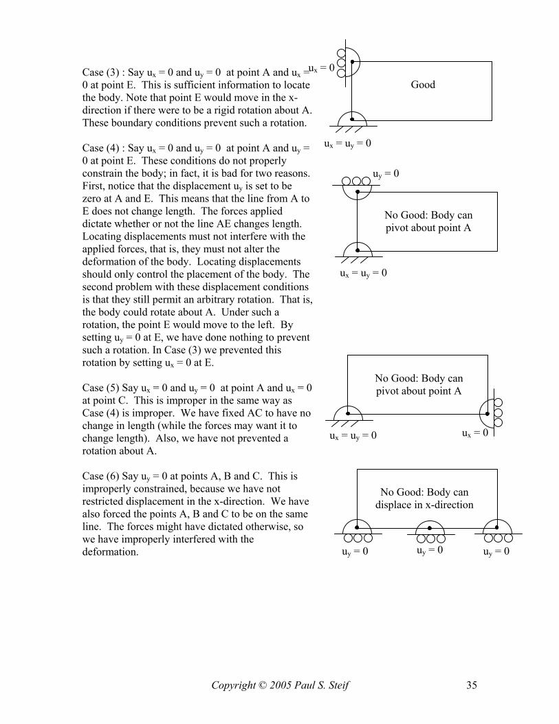
Case (3) : Say ux = 0 and uy = 0 at point A and ux = 0 at point E. This is sufficient information to locate the body. Note that point E would move in the x-direction if there were to be a rigid rotation about A. These boundary conditions prevent such a rotation. Case (4) : Say ux = 0 and uy = 0 at point A and uy = 0 at point E. These conditions do not properly constrain the body; in fact, it is bad for two reasons. First, notice that the displacement uy is set to be zero at A and E. This means that the line from A to E does not change length. The forces applied dictate whether or not the line AE changes length. Locating displacements must not interfere with the applied forces, that is, they must not alter the deformation of the body. Locating displacements should only control the placement of the body. The second problem with these displacement conditions is that they still permit an arbitrary rotation. That is, the body could rotate about A. Under such a rotation, the point E would move to the left. By setting uy = 0 at E, we have done nothing to prevent such a rotation. In Case (3) we prevented this rotation by setting ux = 0 at E. Case (5) Say ux = 0 and uy = 0 at point A and ux = 0 at point C. This is improper in the same way as Case (4) is improper. We have fixed AC to have no change in length (while the forces may want it to change length). Also, we have not prevented a rotation about A. Case (6) Say uy = 0 at points A, B and C. This is improperly constrained, because we have not restricted displacement in the x-direction. We have also forced the points A, B and C to be on the same line. The forces might have dictated otherwise, so we have improperly interfered with the deformation.
Good
ux = uy = 0
ux = 0
No Good: Body can pivot about point A
ux = uy = 0
uy = 0
No Good: Body can pivot about point A
ux = uy = 0 ux = 0
No Good: Body can displace in x-direction
uy = 0 uy = 0 uy = 0
Copyright © 2005 Paul S. Steif 36
5. EXAMINING THE RESULTS OF FEA There are many opportunities to make errors when using FEA. For this reason, experienced analysts check their FEA results in a number of ways. Deformed Mesh Look at deformed mesh. While you cannot judge whether the details are right, the gross change in shape or the deflection should be sensible. In particular, look at those parts of the boundary where you set the displacements (to be zero or otherwise). The deformed mesh should be consistent with those displacements that you intended to set. Boundary Values of Stress On those parts of the boundary that are supposed to be free, certain stress components, or combinations of stress components, should ideally be zero. This was discussed in the Chapter on Equations of Elasticity. Now, because of the approximate method used by most finite element programs, these boundary conditions involving force (or lack of force) may not be precisely satisfied. (By contrast, when you prescribe displacements to be zero or otherwise, the finite element results will be precisely correct for those displacements.) Nevertheless, the stresses (or appropriate combinations of stresses) at the free boundaries should be small at least compared with stresses generally prevailing in the body. The magnitude of those stresses relative to the generally prevailing stresses gives some indication of the overall accuracy of the finite element solution. Mesh Refinement For some very simple problems, such as uniaxial tension, the finite element program can give correct results even with a very coarse mesh of few elements. However, in general, one looks for the results for stresses and displacements to change as the mesh is changed. Now, we assume the problem being analyzed does not have a stress singularity (see the Chapter on Stress Concentrations and Singularities). In this case of no stress singularity, the stresses should appear to approach values as the number of mesh points increases. Of course, it is important for there to be many mesh points in the region of high stress gradients (Stress Concentrations). Convergence of the stress is the way of discerning whether you have refined the mesh enough. You could still have the wrong answer, if you incorrectly translated the physical problem into a finite element analysis (e.g., wrong boundary conditions) or if you did not input what you intended. Thus, mesh refinement does not replace the checks discussed above and below.
Copyright © 2005 Paul S. Steif 37
Comparing Finite Element Results with the Results of Another Analysis
Comparing the results of a finite element analysis with a simpler calculation is the most powerful way to judge whether finite element results are sensible. The simpler calculation could be just a rough hunch as to the level of the stresses (based on overall loads and areas). It could also be a full-blown mechanics of materials solution. Sometimes one expects the mechanics of materials solution to give just a crude prediction of stresses. Other times, one expects the mechanics of materials solution to give highly accurate stresses. A crude estimate can help to point out a gross error in the FEA input, which makes the stress incorrect by orders of magnitude. Comparison with more accurate estimates may give an indication of more subtle errors in the FEA. How do you estimate stresses? There is no single simple approach for estimating stresses. Engineers who devote themselves to this subject hone their ability to do so over a lifetime. Such engineers have familiarity with many exact and approximate solutions from elasticity theory, as well as mechanics of materials. However, engineers with only a background in mechanics of materials are increasingly going on to use FEA. The following is intended to be helpful to such engineers. We are presuming that the engineer can make use of the analyses of axial loading, bending, and torsion for various cross-sections. Such analyses can give highly accurate results in certain circumstances and less accurate results in other circumstances. For the mechanics of materials theories to give highly accurate results for stresses, all the following conditions must be satisfied: The portion of the body of interest is straight with an unchanging cross-section (a
prismatic bar). Alternatively, that part of the body must have a cross-section that changes very slowly as you move along its length.
The sides of the bar are unloaded or the loading of the sides of the bar is distributed,
preferably uniformly or with a very gradually varying distribution. The cross-section at which the stresses are being evaluated is “far” from the regions at
which the loads are applied. “Far” means that the cross-section is a distance of several “h” away from the loading, where h is a lineal dimension of the cross-section.
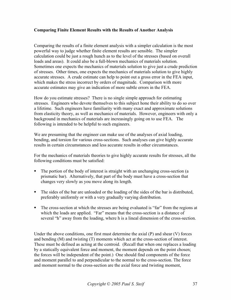
Under the above conditions, one first must determine the axial (P) and shear (V) forces and bending (M) and twisting (T) moments which act at the cross-section of interest. These must be defined as acting at the centroid. (Recall that when one replaces a loading by a statically equivalent force and moment, the moment depends on the point chosen; the forces will be independent of the point.) One should find components of the force and moment parallel to and perpendicular to the normal to the cross-section. The force and moment normal to the cross-section are the axial force and twisting moment,
Copyright © 2005 Paul S. Steif 38
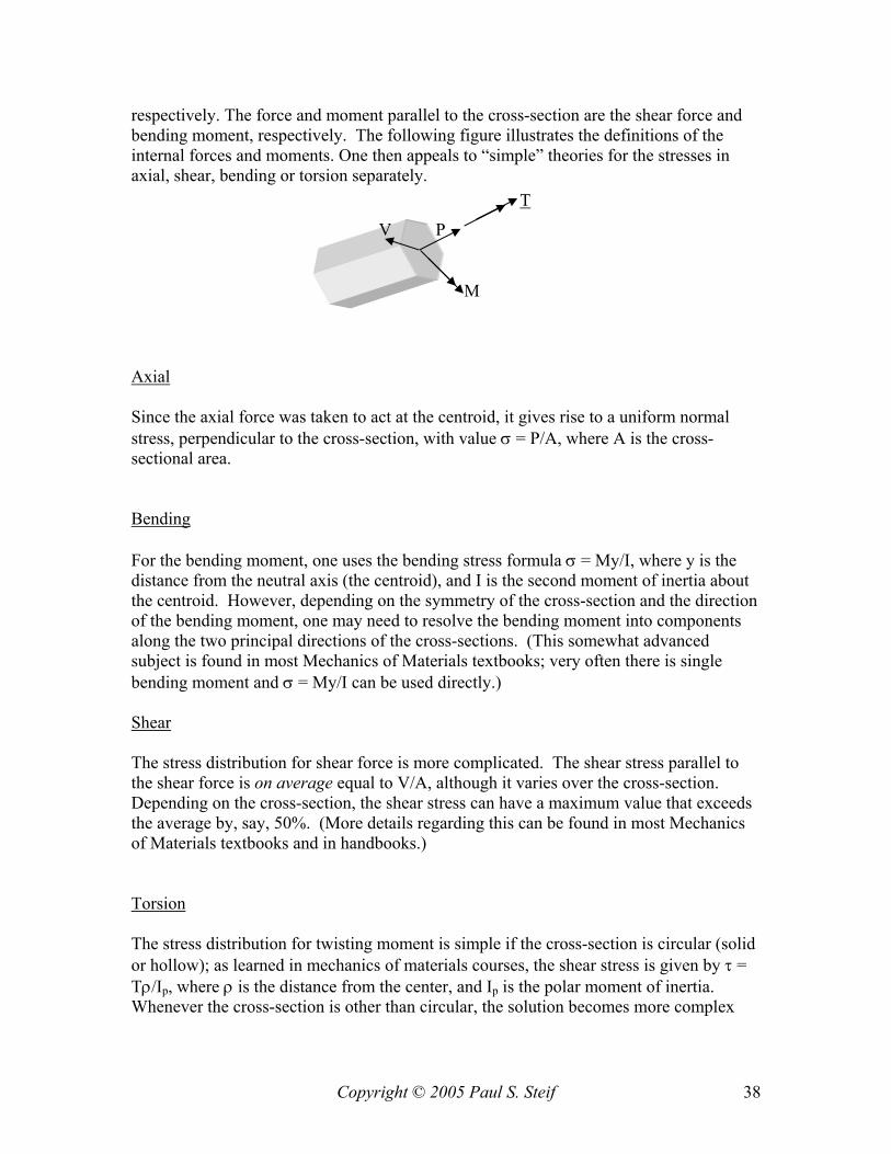
respectively. The force and moment parallel to the cross-section are the shear force and bending moment, respectively. The following figure illustrates the definitions of the internal forces and moments. One then appeals to “simple” theories for the stresses in axial, shear, bending or torsion separately. Axial Since the axial force was taken to act at the centroid, it gives rise to a uniform normal stress, perpendicular to the cross-section, with value σ = P/A, where A is the cross-sectional area. Bending For the bending moment, one uses the bending stress formula σ = My/I, where y is the distance from the neutral axis (the centroid), and I is the second moment of inertia about the centroid. However, depending on the symmetry of the cross-section and the direction of the bending moment, one may need to resolve the bending moment into components along the two principal directions of the cross-sections. (This somewhat advanced subject is found in most Mechanics of Materials textbooks; very often there is single bending moment and σ = My/I can be used directly.) Shear The stress distribution for shear force is more complicated. The shear stress parallel to the shear force is on average equal to V/A, although it varies over the cross-section. Depending on the cross-section, the shear stress can have a maximum value that exceeds the average by, say, 50%. (More details regarding this can be found in most Mechanics of Materials textbooks and in handbooks.) Torsion The stress distribution for twisting moment is simple if the cross-section is circular (solid or hollow); as learned in mechanics of materials courses, the shear stress is given by τ = Tρ/Ip, where ρ is the distance from the center, and Ip is the polar moment of inertia. Whenever the cross-section is other than circular, the solution becomes more complex
P V
M
T
Copyright © 2005 Paul S. Steif 39
and is not treated in most Mechanics of Materials textbooks. However, the solution can be found in textbooks on elasticity and in handbooks. Besides being able to calculate stresses for prismatic materials, it is important to know which of the six three-dimensional stress components correspond to the above calculations. For axial and bending loads, the stress is the normal stress acting perpendicular to the cross-section. In the case of a shear force, the maximum shear stress acts in the direction of V. In the case of the twisting moment, the maximum shear stress acts tangential to the free surface. Crude Estimates of Stress from Mechanics of Materials Often the conditions set forth above are not satisfied. The body is not prismatic, or there are concentrated lateral loads or the cross-section is not far from the applied loads. The mechanics of materials theories can still be applied, although their estimates of the stress may be more or less in error, depending on how seriously the conditions are violated. To apply these theories to a point in the body, imagine a plane intersecting that point and passing through the whole body. It is preferable to choose the plane to be perpendicular to the free surface of the body, although that is often not possible. This plane separates the body into two portions. Imagine further that statics is used to find the net force and moment transmitted through that plane. You could find this net force and moment if you knew the forces acting on one or the other of the two portions of the body. One then proceeds to use the above theories of axial loading, bending, shear and torsion with the given loading and the cross-section that has been intersected.
Original body with plane passing through cross-
section of interest
Part of original body body with net force and moment
acting on cross-section