Notes on Independent Component AnalysisJon Shlens

5 August 2002

II. Review: pdf, cdf and Entropya. Probability Density Functions (pdf) and Cumulative Density Functions (cdf)

• Abandon knowledge of the temporal / presentation order in time series data• 3 pdf’s of interest: exponential, Gaussian, uniform• cdf is the integral of the pdf

Note: Technically pdf of exponential distribution is only defined for x>0

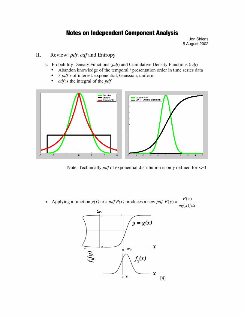
b. Applying a function g(x) to a pdf P(x) produces a new pdf

†

P(y) =P(x)

∂g(x) ∂x

[4]

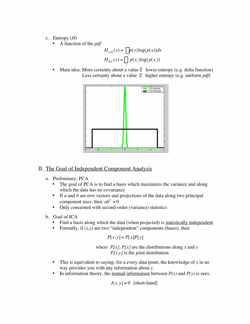
c. Entropy (H)• A function of the pdf

†

Hcont (x) = p(x)log(p(x))dxÚHdisc (x) = p(xi)log(p(xi))

iÂ

• Main idea: More certainty about a value ‡ lower entropy (e.g. delta function) Less certainty about a value ‡ higher entropy (e.g. uniform pdf)

II. The Goal of Independent Component Analysisa. Preliminary: PCA

• The goal of PCA is to find a basis which maximizes the variance and alongwhich the data has no covariance

• If a and b are row vectors and projections of the data along two principalcomponent axes, then

†

abT = 0• Only concerned with second-order (variance) statistics

b. Goal of ICA• Find a basis along which the data (when projected) is statistically independent• Formally, if (x,y) are two “independent” components (bases), then

†

P[x, y] = P[x]P[y]

where P[x], P[x] are the distributions along x and y P[x,y] is the joint distribution

• This is equivalent to saying: for a every data point, the knowledge of x in noway provides you with any information about y.

• In information theory, the mutual information between P(x) and P(y) is zero.

†

I(x, y) = 0 [short-hand]

c. Why neuroscience?• Several papers have conjectured that the goal of cortical processing is

redundancy reduction [1,2]• “the activation of each feature detector is supposed to be as statistically

independent from the others as possible” [5]

III. Several Solutions to ICA

a. Expectation Maximization (EM) with Maximum Likelihood Estimation (MLE)• Dayan and Abbott; difficult to understand.

b. Other methods• Kurtosis maximization: http://www.cs.toronto.edu/~roweis/kica.html• Projection pursuit: http://www.cis.hut.fi/aapo/papers/IJCNN99_tutorialweb/

c. Information maximization• The Bell and Sejnowski formulation

IV. Framework for ICA

a. Set-up (2 signal example)• An unknown set of statistically independent signals: S• An unknown mixing matrix: A

†

A =1 0-1 1

Ê

Ë Á

ˆ

¯ ˜

†

S =

| |signal1 signal2

| |

Ê

Ë

Á Á Á

ˆ

¯

˜ ˜ ˜

• Assume the data we receive X is a mixture of the original signals

†

X =

| |mixed1 mixed2

| |

Ê

Ë

Á Á Á

ˆ

¯

˜ ˜ ˜

= AS

• Because X is a mixture of signals, the mixed components (e.g. mixed1, mixed2)are not statistically independent.

b. The ICA Question• Can we recover A and S just from X?• Mathematically, can we find a matrix W such that:

†

U = WX

where

†

AW = I or equivalently,

†

U = S

• (Yes. By finding the basis vectors A that are statistically independent.)

c. The Discovery / Trick: Information Maximization

• The Main Goal: Maximize the joint entropy of

†

Y = g(U) where g is a sigmoidfunction

†

g(x) = 11+e - x

1. Find a matrix W such that:

†

max H(g(WX)){ }2. The matrix W becomes the inverse of A. (

†

W = A-1)3. Side note: We are coincidentally maximizing the mutual information

between X and Y if we assume our model does not magnify the entropy ofthe noise. [5]

• An intuitive algorithm to implement this:

1. Define a surface

†

H(g(WX))

2. Find the gradient

†

∂∂W

H(...) and ascend it!

3. When the gradient is zero, done.

V. Proof of Information Maximization: Why does this work?

a. Notes• This section is basically a rip off of a not-commonly-cited paper [3].• The “Why” is not discussed (fully) in the original papers [4,5]• Also, for my convenience I am being “fast and loose” with my notation.

Namely,

†

yi could mean the “distribution of

†

yi” (technically denoted

†

P(yi) orjust the variable

†

yi.

b. THE PROOF

1. If the columns of U are statistically independent, applying an invertibletransformation

†

Y = g(U) can not make them dependent.

†

I(ui,u j ) = 0 fi I(yi,y j ) = 0 where ui and yj are the columns of U and Y

2. The individual entropies

†

H(yi) are maximized when the distribution of

†

yi isthe cdf of the distribution of ui (the pdf).

•

†

H(yi) is maximum when

†

yi = g(ui) is the uniform distribution• By review section (b), we can equate:

†

P(yi) =P(ui)

∂yi ∂ui

1=P(ui)

∂yi ∂ui

yi = P(ui)duÚ

[4]Note: At wopt the output distribution becomes uniform and the sigmoid

aligns to become the cdf of the input distribution.

3. The joint entropy of two sigmoidally-transformed outputs

†

H(y1,y2) ismaximal when

†

y1, y2 are statistically independent and g is the cdf of

†

u1,u2 .• Remember the definition of joint entropy

†

H(y1,y2) = H(y1) + H(y2) - I(y1,y2)

• The mutual information is minimized (equal to zero) when

†

y1,y2 arestatistically independent.

• Via step 2, we know that that

†

H(yi) is maximized when the sigmoid isthe cdf of ui

4. When one combines 2 non-Gaussian pdf’s, the new pdf is more Gaussian.• This is the Central Limit Theorem.

5. FINAL POINT: The big one!

• Reconsider the joint entropy for two variables:

†

H(y1,y2)• This quantity is maximized when

†

y1,y2 are statistically independent andwhen g is the cdf of ui. By Step 1, this statement is equivalent torequiring

†

u1,u2 be statistically independent. Hence, it must be that

†

ui = signali!• If there is any deviation from this causing a mixing of the signals, then:

i. There exists a statistical dependency between the ui. Thisincreases

†

I(ui,u j ), increasing

†

I(g(ui),g(u j )) and thusdecreasing the joint entropy.

ii. There is a decrease in the individual entropies

†

H(yi) as theindividual distributions

†

yi deviate from a uniform distribution(via Step 4 and Step 2). This also decreases the joint entropy.

• Therefore, maximizing the joint entropy is equivalent to

†

ui = signali .

c. Problems with Information Maximization

1. The cdf must be able to “match” the pdf of the signal distributions (

†

signali).• One must use a judicious choice of non-linearity• The sigmoid works well in practice for super-Gaussian (or positive

kurtosis) distributions. Surprisingly, in practice the distribution of mostreal-world sensory input has a high kurtosis. [See figure 5 in 5]

2. There can not be more than one Gaussian source. There is no statisticalinformation to “pull” these distributions apart because of the Central LimitTheorem.

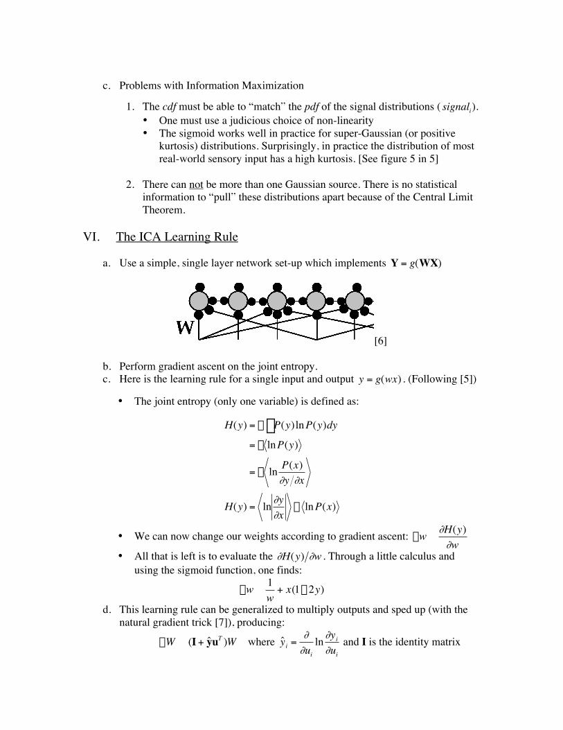
VI. The ICA Learning Rule

a. Use a simple, single layer network set-up which implements

†

Y = g(WX)

[6]

b. Perform gradient ascent on the joint entropy.c. Here is the learning rule for a single input and output

†

y = g(wx) . (Following [5])

• The joint entropy (only one variable) is defined as:

†

H(y) = - P(y)ln P(y)dyÚ= - lnP(y)

= - ln P(x)∂y ∂x

H(y) = ln ∂y∂x

- ln P(x)

• We can now change our weights according to gradient ascent:

†

Dw µ∂H(y)

∂w• All that is left is to evaluate the

†

∂H(y) ∂w . Through a little calculus andusing the sigmoid function, one finds:

†

Dw µ1w

+ x(1- 2y)

d. This learning rule can be generalized to multiply outputs and sped up (with thenatural gradient trick [7]), producing:

†

DW µ (I + ˆ y uT )W where

†

ˆ y i =∂

∂ui

ln∂yi

∂ui

and I is the identity matrix

e. General comments• A competition between an “anti-Hebbian” (first) term and a “Hebbian”

(second) term.• The learning rule is global (not local) making it not biologically plausible in

its current mathematical form.• … although many believe ICA is begin performed somewhere (e.g. primary

visual cortex [5]) but using a different mathematical form.

VII. References

[1] Barlow, H (1989) “Unsupervised Learning” Neural Computation 1, 295-311.

[2] Atick JJ (1992) “Could information theory provide an ecological thery of sensoryprocessing?” Network 3, 213-251.

[3] Bell A. and Sejnowski (1995) “Fast blind separation based on information theory.”Proceedings of the International Symposium on Nonlinear Theory and Applications.[Available at ftp://ftp.cnl.salk.edu/pub/tony/nolta3.ps.Z]

[4] Bell A.J. and Sejnowski T.J. (1995). An information maximization approach to blindseparation and blind deconvolution, Neural Computation, 7, 6, 1129-1159.

[5] Bell A.J. and Sejnowski T.J. (1996). The `Independent Components' of natural scenesare edge filters, to appear in Vision Research

[6] Dayan, Abbott (1999) Theoretical Neuroscience: MIT Press.

[7] Amari et al (1996) “A new learning algorithm for blind signal separation.” Advancesin neural information processing systems (Vol 8). Cambridge, MA: MIT Press.