NOTES ON MACDONALD POLYNOMIALSAND THE GEOMETRY OF HILBERT … · 2 1.2. HISTORY In 1988, Macdonald created something of a revolution in the ancient and classical theory of symmetric

NOTES ON MACDONALD POLYNOMIALS AND THE GEOMETRY

OF HILBERT SCHEMES

MARK HAIMAN ([email protected]) ∗U.C. Berkeley

Abstract. These notes are based on a series of seven lectures given in the combinatoricsseminar at U.C. San Diego in February and March, 2001. My lectures at the workshopwhich is the subject of this proceedings volume covered a portion of the same materialin a more abbreviated form.

Key words: Symmetric functions, Macdonald polynomials, Hilbert schemes

2000 Mathematics Subject Classification: Primary 14C05; Secondary 05E05, 14F17, 14M05

1. History and introduction

1.1. OVERVIEW

In these lectures we’ll be discussing a series of new results in combinatorics,algebra and geometry. The main combinatorial problems we solve are (1) weprove the positivity conjecture for Macdonald polynomials, and (2) we provea series of conjectures relating the diagonal harmonics to various familiarcombinatorial enumerations; in particular we prove that the dimension ofthe space of diagonal harmonics is (n+1)n−1. In order to prove these results,we have to work out some new results about geometry of the Hilbert schemeof points in the plane and a certain related algebraic variety. As a technicaltool for our geometric results, in turn, we need to do some commutativealgebra, which although complicated, has a quite explicit and combinatorialnature.

Today I want to give a short history of the original problem and how Igot mixed up in it, and then show you some theorems in three seeminglyunrelated areas. My goal in the remaining lectures will be to explain whatthese theorems have to do with each other and indicate how they are proved.The basic references are the series of four papers [15], [16], [17], and [18](an abbreviated version of the last one appeared as [19]).

∗ Research supported in part by NSF grant DMS-0070772.

2

1.2. HISTORY

In 1988, Macdonald created something of a revolution in the ancient andclassical theory of symmetric functions with the introduction of Macdon-ald polynomials. They are symmetric functions Pµ(x; q, t) in variables x =x1, x2, . . ., with coefficients that are rational functions of two parameters qand t. Their importance stems in part from the fact that by specializingthe two parameters in different ways we recover two previously known andimportant families of symmetric functions involving one parameter: theHall-Littlewood polynomials (by setting q = 0) and the Jack polynomials(by setting t = qα and letting q → 1). After suitably normalizing andtransforming the polynomials Pµ, we get polynomials Hµ(x; q, t), whoseexpansions in terms of Schur functions we may write as

Hµ(x; q, t) =∑

λ

Kλ,µ(q, t)sλ(x).

Here λ and µ are partitions of an integer n. The coefficients Kλ,µ(q, t)are called Kostka-Macdonald coefficients. We’ll define Hµ later. Right nowwe only mention that based on hand calculations, Macdonald conjecturedthat the Kostka-Macdonald coefficients are polynomials with non-negativeinteger coefficients:

Kλ,µ(q, t) ∈ N[q, t].

This is more remarkable for the fact that as defined, the Kλ,µ(q, t) arerational functions of q and t, and were only proved to be polynomials around1996, in five independent papers by a total of seven authors [12, 13, 21, 22,25].

Macdonald defined the coefficients Kλ,µ(q, t) in such a way that onsetting q = 0 (the specialization from Macdonald to Hall-Littlewood poly-nomials) they yield the famous t-Kostka coefficients Kλ,µ(t) = Kλ,µ(0, t).These were known to be in N[t] as a result of a cohomological interpreta-tion due to Hotta and Springer [20, 26], and later a beautiful and subtlecombinatorial interpretation due to Lascoux and Schutzenberger [23]. Bothdescriptions are rather difficult.

When I came to U.C. San Diego in 1991, Adriano Garsia and ClaudioProcesi had been working on a simpler approach to the positivity theoremfor the t-Kostka coefficients [11], with the idea that it might extend tothe q, t case. Adriano and I soon found the right extension—or so weconjectured—but surprisingly, our conjecture defied every attempt at anelementary proof. All that resulted from our attempts was an ever-largerpile of conjectures, notably those on diagonal harmonics alluded to above.Later, we discussed our efforts with Procesi. He was familiar with thegeometry of the Hilbert scheme of points in the plane, and realized that

MACDONALD POLYNOMIALS AND HILBERT SCHEMES 3

there was a way it might explain the diagonal harmonics conjectures. WhatI’ll describe in these lectures is ultimately the result of following up on thissuggestion by Procesi. His proposed set-up eventually turned out to explainthe diagonal harmonics conjectures and, still better and unexpectedly, toexplain our original conjecture on the Kostka-Macdonald coefficients too.

Now let’s turn to our promised list of seemingly unrelated theorems.

1.3. COMBINATORICS/LINEAR ALGEBRA

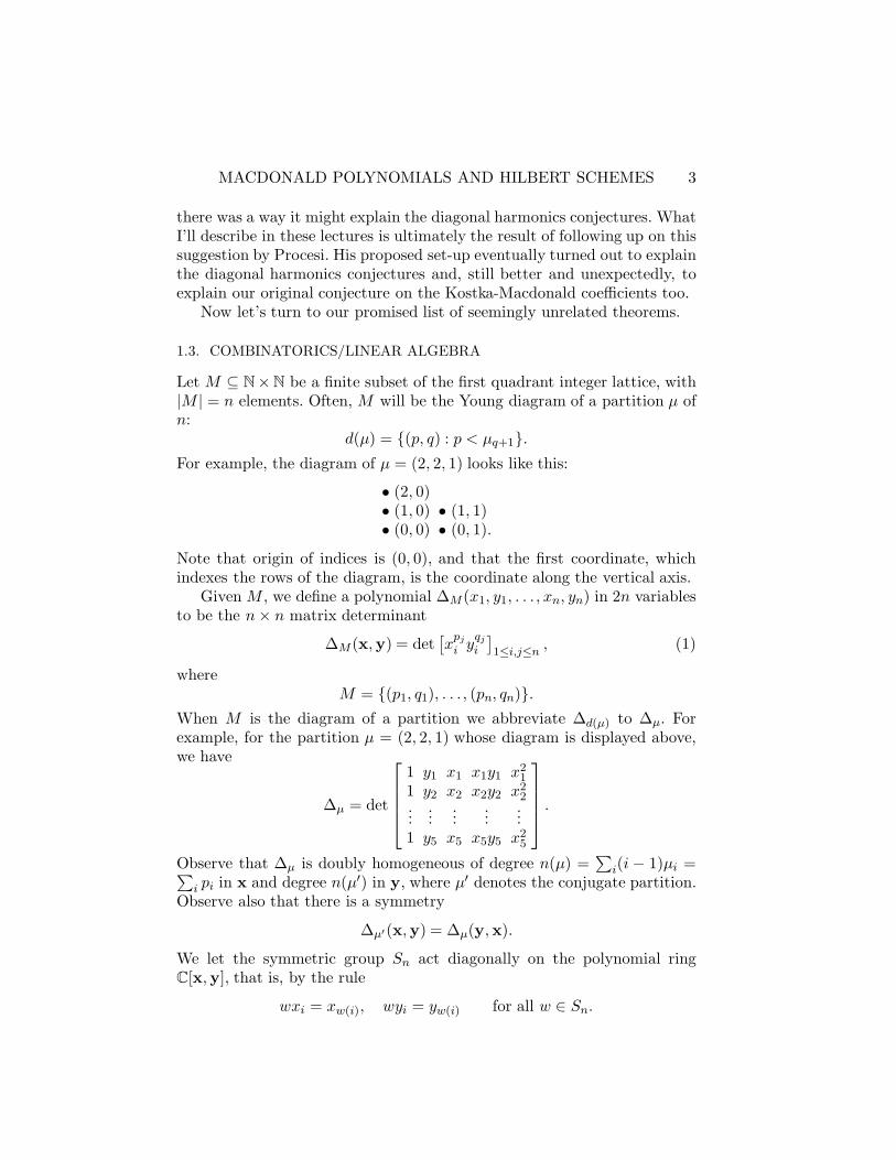
Let M ⊆ N×N be a finite subset of the first quadrant integer lattice, with|M | = n elements. Often, M will be the Young diagram of a partition µ ofn:

d(µ) = {(p, q) : p < µq+1}.For example, the diagram of µ = (2, 2, 1) looks like this:

• (2, 0)• (1, 0) • (1, 1)• (0, 0) • (0, 1).

Note that origin of indices is (0, 0), and that the first coordinate, whichindexes the rows of the diagram, is the coordinate along the vertical axis.

Given M , we define a polynomial ∆M(x1, y1, . . . , xn, yn) in 2n variablesto be the n× n matrix determinant

∆M(x, y) = det[x

pj

i yqj

i

]1≤i,j≤n

, (1)

whereM = {(p1, q1), . . . , (pn, qn)}.

When M is the diagram of a partition we abbreviate ∆d(µ) to ∆µ. Forexample, for the partition µ = (2, 2, 1) whose diagram is displayed above,we have

∆µ = det

1 y1 x1 x1y1 x21

1 y2 x2 x2y2 x22

......

......

...1 y5 x5 x5y5 x2

5

.

Observe that ∆µ is doubly homogeneous of degree n(µ) =∑

i(i− 1)µi =∑i pi in x and degree n(µ′) in y, where µ′ denotes the conjugate partition.

Observe also that there is a symmetry

∆µ′(x, y) = ∆µ(y, x).

We let the symmetric group Sn act diagonally on the polynomial ringC[x, y], that is, by the rule

wxi = xw(i), wyi = yw(i) for all w ∈ Sn.

4

Then Sn permutes the rows of the matrix in (1), hence acts on ∆M by

w∆M = ε(w)∆M ,

where ε is the sign character. In other words, ∆M is an alternating polyno-mial. Given any monomial xpyq = xp1

1 yq11 · · ·xpn

n yqnn with distinct exponents

(pi, qi), the alternation of xpyq is ±∆M for the corresponding M . If theexponents are not distinct, then the alternation of the monomial xpyq iszero. From this it is not hard to see that the set of all determinants ∆M

is a basis of the space of alternating polynomials C[x, y]ε. Another wayto see this is by identifying C[x, y]ε with the exterior power ∧nC[x, y].Then the determinants ∆M are identified with the basis given by wedgesof monomials xpyq ∈ C[x, y].

Now, given a partition µ of n, consider the space spanned by all iteratedpartial derivatives of ∆µ

Dµ = C[∂x, ∂y]∆µ.

This space is

− finite dimensional,− closed under differentiation (i.e., it’s a Macaulay inverse system),− Sn-invariant, and− doubly graded: Dµ =

⊕r,s(Dµ)r,s,

where (Dµ)r,s is the subset of doubly homogeneous polynomials in Dµ ofdegree r in x and s in y. The Sn action on Dµ respects the double grading.

THEOREM 1.1. We have dimDµ = n!, and Sn acts on Dµ by the regularrepresentation.

A refinement of this theorem describes the Sn action on each doublyhomogeneous component (Dµ)r,s individually. Recall that every Sn-moduleis a direct sum of irreducible ones, and that the irreducible Sn-modules V λ

(up to isomorphism) are indexed by partitions λ of n. The character of anSn-module will be denoted chV . The irreducible characters are χλ = chV λ.The multiplicity of χλ in an arbitrary character φ is denoted 〈χλ, φ〉.

THEOREM 1.2. The generating function for the multiplicty of χλ in thecomponents (Dµ)r,s is given by

∑r,s

trqs〈χλ, ch(Dµ)r,s〉 = Kλ,µ(q, t),

the Kostka-Macdonald coefficient.


The character multiplicities in the above formula are of course non-negative integers, so this proves the Macdonald positivity conjecture.

COROLLARY 1.3. (Conjecture, Macdonald 1988). We have Kλ,µ(q, t) ∈N[q, t].

Example (the classical case). Take µ = (1n). The diagram of (1n) is

• (n− 1, 0)...• (1, 0)• (0, 0)

Notice that the y variables have exponent zero in the determinant ∆(1n),while the x variables form the Vandermonde matrix. Thus we have

∆(1n) = ∆(x) =∏i<j

(xi − xj),

the Vandermonde determinant. Now let

I = {f(x) : f(∂x)∆(x) = 0}be the annihilating ideal of the inverse system generated by ∆(x). It isequal to the ideal generated by all Sn-invariant polynomials in x withoutconstant term, or just by the power-sums pk =

∑ni=1 x

ki , that is,

I = (C[x]Sn+ ) = (p1, . . . , pn).

We have isomorphisms of graded Sn-modules

D(1n)∼= C[x]/I ∼= H∗(GLn/B).

On the far right here we have the cohomology ring of the flag variety forGLn, which is well-known to have dimension n! and to carry the regularrepresentation of Sn. A corresponding result holds for any semi-simplecomplex Lie group and its Weyl group.

The spaces Dµ provide one kind of bivariate, doubly graded generaliza-tion of the above classical example. Another way to get such a generalizationis to consider the Macaulay inverse system defined by the bivariate analogof the ideal I . Thus we set

J = (C[x, y]Sn+ ) = (ph,k : 1 ≤ h+ k ≤ n).

Here ph,k =∑n

i=1 xhi y

ki is a polarized power-sum; they generate J by a

theorem of Weyl. The ideal J defines a Macaulay inverse system

DHn = {q ∈ C[x, y] : f(∂x, ∂y)q = 0 for all f ∈ J}.

6

Or, more simply, DHn is the solution space of the system of differentialequations ph,k(∂x, ∂y)q = 0. We have

DHn∼= C[x, y]/J

as (doubly) graded Sn-modules, so for character considerations the two areinterchangable. The ring on the right is the ring of coinvariants for thediagonal action of Sn. The space DHn is the space of harmonics for thisaction, or diagonal harmonics.

THEOREM 1.4. We have dimDHn = (n+ 1)n−1.

This theorem also has a refinement giving the character of (DHn)r,s inevery degree r, s. The formula involves Macdonald polynomials and will bepresented later. Garsia and I conjectured the above theorem around 1992.Shorty afterwards we and others including Gessel and Stanley found variouscombinatorial refinements to the conjecture. For example, (n+1)n−1 countsrooted forests on the vertex set {1, . . . , n}. If we only look at the gradingof DHn by x-degree, we find that dim(DHn)d,− is the number of rootedforests with d inversions (a pair of vertices i < j is an inversion if j ison the path connecting i to the root of its tree). As another example, thedimension of the space DHε

n of alternating diagonal harmonics turns outto be the Catalan number Cn. A full discussion of these various conjecturescan be found in [14].

Armed with Procesi’s idea about the underlying geometry, I was even-tually able to conjecture the full character formula for DHn. Garsia andI then succeeded in proving that all the combinatorial conjectures wouldfollow from the master formula [10]. The proof is based on the knownspecializations of Macdonald polynomials for q = 1 and for q = t, plus alot of work with symmetric function identities and Garsia’s theory of q-Lagrange inversion. This is very beautiful, but could take several lecturesin itself, so I won’t delve further into it.

1.4. ALGEBRAIC GEOMETRY

We denote byHn = Hilbn(C2)

the Hilbert scheme of points in the affine plane C2. It is an algebraic varietywhich parametrizes finite subschemes of length n in C2. You don’t reallyneed to know what those words mean, because (by definition) such sub-schemes correspond one-to-one with certain ideals in the coordinate ringof C2, and I’m going to tell you which ones they are. The coordinate ring


of C2 is of course the ring R = C[x, y] of polynomials in the coordinatefunctions x and y. We can describe the Hilbert scheme set-theoretically as

Hn = {I ⊆ R : dimCR/I = n}.Thus the relevant ideals are those for which R/I is a finite-dimensionalvector space, of dimension n. In more geometric language, R/I has Krulldimension zero, and length n. For such an ideal I , the locus V (I) ⊆ C2

defined by the vanishing of all polynomials in I is finite, with at most npoints. But V (I) may have fewer than n points, and then the local rings(R/I)P at these points may be non-reduced (they may contain non-zeronilpotent elements) and have length greater than 1. Defining the multiplicityof R/I at P to be the length of the local ring (R/I)P , the sum of themultiplicities is always equal to n. The multiplicities do not determine I ingeneral, so a point of Hn carries with it more information than just the setV (I) and the multiplicities of its elements.

Examples. (1) The “generic” example of a point ofHn is the ideal I = I(S)of all polynomials which vanish on a specified finite subset S ⊆ C2 of size|S| = n. In this case, I is a radical ideal and R/I is reduced. Each point in Shas multiplicity one, and R/I can be identified with the ring of polynomialfunctions on S. Since S is finite, every function is a polynomial function,so R/I ∼= CS ∼= Cn, showing that I(S) is a legitimate element of Hn.

(2) The “most special” examples of points of Hn are the monomialideals. Let µ be a partition of n, and let

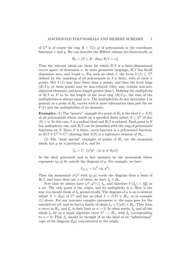
Iµ = C · {xpyq : (p, q) 6∈ d(µ)}be the ideal generated, and in fact spanned, by the monomials whoseexponents (p, q) lie outside the diagram of µ. For example, we have

I(3,1) = (x2, xy, y3).

Then the monomials xpyq with (p, q) inside the diagram form a basis ofR/I , and since there are n of them, we have Iµ ∈ Hn.

Note that we always have (xn, yn) ⊆ Iµ, and therefore V (Iµ) = {0} asa set. The only point is the origin, and its multiplicity is n. Here is theway you should think of Iµ geometrically. The diagram of µ is an n-elementsubset S = d(µ) of C2 and has an ideal I = I(S) ∈ Hn, as in example(1) above. For any non-zero complex parameter u, the same goes for therescaled set uS, and we have a family of ideals Iu = I(uS) ∈ Hn. They forma curve in Hn, and Iµ is their limit as u→ 0. In other words, Iµ and all theideals Iu lie on a single algebraic curve C1 ↪→ Hn, with Iµ correspondingto u = 0. Thus Iµ should be thought of as the ideal of an “infinitesimal”copy of the diagram d(µ) concentrated at the origin.

8

We haven’t yet said anything about the structure of Hn as an algebraicvariety, that is, about how it acquires local coordinates. Roughly speaking,its coordinates are defined similarly to the Plucker coordinates on a Grass-mann variety. This will be explained in more detail later. For now, let’saccept that it has a natural variety structure. It is a very special variety,as indicated by the following famous and remarkable theorem.

THEOREM 1.5. (Fogarty [7]). The Hilbert scheme Hn is non-singular andirreducible, of dimension 2n.

This theorem does not hold for the Hilbert scheme of points in Cd whend > 2. We may mention here also that the “n!” theorem, Theorem 1.1,does not hold in more than two sets of variables x, y, . . . , z, and these twophenomena are connected with each other. One reason why elementaryattempts to prove the n! theorem have failed so far is that most ideas onethinks of are equally applicable to three or more sets of variables—andtherefore must be wrong. In the geometric proof, the critical ingredientthat causes it to break down beyond the bivariate case is the role of Hn.

We remark that the irreducibility aspect of Forgarty’s theorem meansthat the ideals I = I(S) in example (1) above are truly “generic,” in thatthey form a dense (open) subset of Hn. Thus every I ∈ Hn can be realizedas a limit of ideals I(S), somewhat as we did above for Iµ (but not alwaysby a rescaling; that only gives the homogeneous ideals).

There is a map

σ:Hn → SnC2,

where SnC2 = C2n/Sn is the variety of unordered n-tuples JP1, . . . , PnK ofpoints in C2. It is defined by

σ(I) = Jm1 · P1, . . . , mk · PkK,

where V (I) = {P1, . . . , Pk} and mi = length(R/I)Pi is the multiplicity ofPi. The map σ is called the Chow morphism, and is a morphism of algebraicvarieties (in fact, a projective morphism). Note that for JP1, . . . , PnK ∈SnC2 with all Pi distinct, there is a unique I ∈ Hn such that σ(I) =JP1, . . . , PnK, namely I = I(S), where S = {P1, . . . , Pn}. Thus the Chowmorphism is generically one-to-one, or birational, and since Hn is non-singular it is a resolution of singularities of SnC2. Later we will see that itcan also be described as a certain blowup of SnC2.

Now we are ready for one last definition and our next theorem.


DEFINITION 1.6. The isospectral Hilbert scheme Xn is the reduced fiberproduct

Xn −−−→ C2ny yHn

σ−−−→ SnC2.

In other words, Xn is the closed subset {(I, P1, . . . , Pn) : σ(I) = JP1, . . . , PnK}⊆ Hn × C2n, with the induced structure of reduced algebraic variety.

For the experts, we should point out that the scheme-theoretic fiberproduct in this diagram, the closed subscheme of Hn × C2n whose idealsheaf is described by the equations σ(I) = JP1, . . . , PnK, is not reduced. Bydefinition, the ideal sheaf of Xn is the radical of the former ideal sheaf. Wedon’t know how to give explicit local generators of the ideal sheaf of Xn,although we will give an implicit description later on.

THEOREM 1.7. The isospectral Hilbert scheme Xn is normal, Cohen-Macaulay, and Gorenstein.

We’ll discuss the terms normal, Cohen-Macaulay and Gorenstein later,when they are needed. For now, they just mean that Xn, although singular,has only very special singularities.

1.5. COMMUTATIVE ALGEBRA

Let E be any space (topological space, algebraic variety, whatever). Wedefine the polygraph Z(n, l) to be the following subset of En × E l:

Z(n, l) ={

(P1, . . . , Pn, Q1, . . . , Ql) : Qi ∈ {P1, . . . , Pn} for all i}.

The reason for the name is as follows. Given a function f : {1, . . . , l} →{1, . . . , n}, define the map

πf :En → E l

πf (P1, . . . , Pn) = (Pf(1), . . . , Pf(l)).

Its graph is the locus Wf ⊆ En × E l defined by

Wf = {(P1, . . . , Pn, Q1, . . . , Ql) : Qi = Pf(i) for all i}.Clearly Z(n, l) =

⋃f Wf is the union of these graphs, hence “polygraph.”

Now fix E = C2 and fix coordinates on En ×E l = C2n+2l

x, y, a,b = x1, y1, . . . , xn, yn, a1, b1, . . . , al, bl.

10

In coordinates, Wf is the linear subspace, and algebraic subvariety, definedby the equations

Wf = V (If ), If = (ai − xf(i), bi − yf(i) : 1 ≤ i ≤ l).

Therefore Z(n, l) is an arrangement of linear subpaces in C2n+2l, whosecoordinate ring as a (non-irreducible) algebraic variety is

R(n, l) = C[x, y, a,b]/I(n, l),

where I(n, l) =⋂

f If is the ideal of all polynomials vanishing on Z(n, l)(or equivalently, vanishing on Wf for all f).

THEOREM 1.8. For E = C2, the coordinate ring R(n, l) of the polygraphZ(n, l) is a free C[y]-module.

By symmetry we could equally well have said that R(n, l) is a free C[x]-module. The point is that it’s free over the polynomial ring in either one ofthe two sets of coordinates on C2n.

1.6. CONCLUSION

We close with a hint as to the relationships between the various theoremsdiscussed above, and an outline of the remaining lectures. We shall see thatthe n! theorem is a consequence of the theorem on the geometry of Xn,Theorem 1.7. We can already indicate how the two are connected. BecauseHn is nonsingular and the projection ρ:Xn → Hn is finite, the Cohen-Macaulay property of Xn is equivalent to ρ being flat. This means thatits scheme-theoretic fibers have constant length. Now for a generic pointI = I(S) in Hn, with S = {P1, . . . , Pn}, the fiber of ρ over I consists ofthe points (I, Pw(1), . . . , Pw(n)), where (Pw(1), . . . , Pw(n)) is one of the n!possible orderings of the points of S. These generic fibers can be identifiedwith reduced, regular Sn-orbits in C2n, and have length n!. By flatness,every fiber has length n!, and carries the regular representation of Sn on itscoordinate ring (the Sn-character is constant, as well as the length). SinceV (Iµ) = {0}, the fiber of ρ over Iµ is (set-theoretically) concentrated at aunique point Qµ = (I, 0, . . . , 0) ∈ Xn. The coordinate ring of the scheme-theoretic fiber is a non-reduced local ring of the form Rµ = C[x, y]/Jµ, oflength n! and carrying the regular representation of Sn. It turns out thatthe ideal Jµ is exactly the annihilating ideal of the Macaulay inverse systemDµ, so that Rµ and Dµ are isomorphic as doubly-graded Sn-modules.

The proof of Theorem 1.7 is mostly geometric. Beginning with the nextlecture, we will work out some basic descriptive facts about Hn, Xn and anested Hilbert scheme Hn−1,n to be introduced later, and then go through


this geometric proof. At one point, however, we will assume a technicalresult: that the composite projection Xn → C2n → Cn, where the secondmap is projection on the y coordinates, is flat. To justify this we needthe polygraph theorem, Theorem 1.8. We will see that Xn is a blowup ofC2n, and using Theorem 1.8, we will see that the Rees algebra defining theblowup is a free C[y]-module. This implies the required flatness result.

The proof of the polygraph theorem has a completely different flavorfrom the geometric argument, and we will come to it afterwards. In essence,it is simple: to prove that R(n, l) is a free C[y]-module, we’ll construct afree module basis. In practice, the inductive procedure for doing this israther horrific. What’s worse, the algorithm by which we construct the basiselements does not immediately show that they are in R(n, l) at all! We willconstruct them as functions on Z(n, l), but not obviously as regular func-tions, i.e., functions defined by polynomials. So as an added complicationwe must prove as we go along that our basis elements are regular functions.We will not go through every detail of the proof in these lectures. What Iwill try to do is show you enough of the general framework and method ofthe construction so that you can more easily follow the details in [17], ifyou are interested.

What I will also try to show you, which is not in [17], is that thebasis construction has some beautiful combinatorics. Specifically, the basiselements will be indexed by simple combinatorial data from which youcan read off their degrees (like everything in this story, they are doublyhomogeneous) and other identifying information. As a consequence we get acombinatorial interpretation of the doubly graded Hilbert series An,l(q, t) ofthe ring R(n, l). This has the remarkable feature that although the Hilbertseries has an obvious symmetry An,l(q, t) = An,l(t, q), the combinatorialdescription is utterly asymmetric. It also has the remarkable feature thatthere is a formula for An,l(q, t) in terms of symmetric function operatorsderived from Macdonald polynomials. There are now many such quantitiesfor which we can prove that the coefficients are non-negative by geometricmeans, but we only have combinatorial interpretations for two of them.One is An,l(q, t), and the other is the q, t-Catalan number Cn(q, t) whosecombinatorial interpetation was discovered by Jim Haglund and proved byhim and Garsia [8, 9]. Apart from the n! theorem, we still have no purelycombinatorial interpretation for Kλ,µ(q, t).

After all this, we will return to Theorem 1.4 and its refinement givingthe full character formula for the diagonal harmonics. This is proved usingthe foregoing geometric results and something new, namely, cohomologyvanishing theorems for tensor powers of the tautological bundle. Our mainresult on Xn can be interpreted (as I will explain) as an isomorphism be-tween Hn and a Hilbert scheme of regular orbits of Sn acting on C2n. Given

12

this isomorphism, we can apply an amazing recent theorem of Bridgeland,King and Reid to completely characterize the derived category of coherentsheaves on Hn. This has the tremendous virtue that it reduces the proofsof the vanishing theorems we need to “mere calculations.” More exactly, itreduces them to calculations that can be done with the aid of the polygraphtheorem! I intend to explain enough of this for you to get a taste of it, butin a sketchier way than the other material, since the sheaf cohomologytechniques will be less accessible to many in the audience than the moreintuitive geometry and commutative algebra involved in the study of Hilbertschemes and polygraphs.

2. Welcome to Hilbert schemes

In this lecture and the next we will explore how the properties of Hn andXn are connected with the n! theorem, and describe Hn and Xn in more el-ementary terms. We will also meet the nested Hilbert scheme Hn−1,n whichwill play a key role in the geometric proof of Theorem 1.7 by induction onn.

2.1. HILBERT SCHEMES AS BLOWUPS

We recall some basics of algebraic geometry. Let R be a reduced (no non-zero nilpotent elements), finitely generated algebra over C. If x1, . . . , xm

generate R, we haveR = C[x]/I,

where I is an ideal such that I =√I . Then R is the ring of regular functions

on the affine algebraic locus

V (I) ⊆ Cn,

that is, its coordinate ring. The locus V (I) can be identified with the setof closed points of a scheme, denoted SpecR. You can and should thinkof SpecR as just another name for the locus V (I)—in the present context(reduced schemes of finite type over C) the two concepts are essentiallyinterchangeable.

A general reduced scheme X of finite type over C is a space which canbe covered by finitely many affine sets U = SpecR for various rings R of theabove kind. The notion of “regular function” on X is defined locally, thatis, the regular functions form a sheaf of rings of functions on X , denotedOX . Thus OX(U) is the ring of regular functions on the open set U . If Uis an affine open set U = SpecR, then OX(U) = R. The ring OX(X) isthe ring of global regular functions defined on all of X . If X is not affine, it


may have few global regular functions: for example, the only global regularfunctions on projective space Pn are the constants.

Next letS = S0 ⊕ S1 ⊕ · · ·

be a graded algebra, generated by S0 and S1. For f ∈ S1 define

Rf = S[f−1]0 = S0[f−1S1] ⊆ S[f−1].

The affine schemes Uf = SpecRf fit together to cover a schemeX projectiveover SpecS0. This scheme is denoted ProjS. For each f , the canonical ringhomomorphism S0 → Rf induces a morphism of affine schemes Uf →Spec S0. We have a canonical projective morphism X → Spec S0, given oneach set Uf by these morphisms.

Examples. (1) Take S = C[x0, . . . , xd] to be a polynomial ring with itsusual grading. We have

Rxi = C[x0/xi, . . . , xd/xi] (xi/xi = 1 omitted),

and Uxi = SpecRxi∼= Cd is the affine d-space with coordinates x0/xi, . . .,

xd/xi. In this caseProjS = Pd

is projective space, and the morphism

ProjS → Spec S0 = Spec C

is the trivial morphism from Pd to a point. A point of Pd given in projectivecoordinates as p = (x0 : x1 : . . . : xd) belongs to the open set Uxi iff xi 6= 0.Then rescaling to make xi = 1, we can write p = (x0/xi : . . . : 1 : . . . :xd/xi), which exhibits x0/xi, . . . , xd/xi as coordinates on Uxi .

(2) If R is a ring and J ⊆ R is an ideal, take

S = R⊕ J ⊕ J2 ⊕ · · · ,the Rees algebra of J. We can identify S with the subring R[tJ] of thepolynomial ring R[t] in an indeterminate t. The morphism

π:X → Y, X = ProjS, Y = SpecR

is the blowup of Y along the subscheme Z = V (J), or the blowup at theideal J. Among its properties:

− The ideal sheaf I ⊆ OX of the subscheme π−1(Z) ⊆ X is locally freeon one generator. Locally on Uf , for f ∈ S1 = J, it is given by theideal I(Uf) = (f) ⊆ Rf . Note that I(Uf) is by definition the idealgenerated by the image of J in Rf , but Rf contains an element g/ffor all g ∈ J, so f generates JRf .

14

− Over the complement W = Y \ Z of Z, the blowup restricts to anisomorphism π−1(W ) ∼= W .

We are going to construct the Hilbert scheme Hn and the isospectralHilbert scheme Xn as blowups. To this end we set

A = C[x, y]ε,

the space of alternating polynomials for the diagonal Sn action on C[x, y] =C[x1, y1, . . . , xn, yn], and let

J = C[x, y]A

be the ideal generated by A. Recall that the polynomials ∆M for all M ⊆N × N, |M | = n form a basis of A, and hence generate the ideal J. Wedefine spaces Ad in the obvious way for d > 0, and set A0 = C[x, y]Sn, toensure that we have

AjAk ⊆ Aj+k,

even when j or k is zero. Note that we also have

Jd = C[x, y]Ad.

THEOREM 2.1. We have

Hn∼= ProjS,

whereS = A0 ⊕A1 ⊕ A2 ⊕ · · · ,

as a scheme over SpecA0 = SnC2, that is, the canonical projective mor-phism for the Proj is the Chow morphism σ:Hn → SnC2. We also have

Xn∼= ProjC[x, y][tJ],

the blowup of C2n at J.

Remarks. (1) For d even, Ad is contained in the ring of invariants A0 =C[x, y]Sn as an ideal, and

S(2) = A0 ⊕A2 ⊕A4 ⊕ · · ·is the Rees algebra of A2. A general fact about the Proj construction isthat ProjS(k) ∼= ProjS, so Hn is the blowup of SnC2 at the ideal A2. Thedescription as ProjS is preferable to the description as the blowup ProjS(2)

because it gives rise to the “correct” ample line bundle O(1) on Hn.(2) The first part of Theorem 2.1 is proved in [15], and the part about

Xn in [17]. In the latter paper I also prove that J is equal to its radical,


which implies the same for A2 = J ∩C[x, y]Sn. In fact J is the ideal of theunion of pairwise diagonals

⋃i6=j

Eij ⊆ C2n, Eij = V (xi − xj , yi − yj),

and A2 is the ideal of its image in SnC2, the set of points JP1, . . . , PnKwith the Pi not all distinct. Thus Hn and Xn are the blowups of SnC2 andC2n respectively, along the pairwise diagonals. This had been expected bygeometers but not proved before.

Example. For n = 2, we have J = (x1 − x2, y1 − y2), and these twogenerators also generate A as an A0-module. The blowup ProjS is thereforecovered by two affines

Ux1−x2 = SpecA0[y1 − y2x1 − x2

], Uy1−y2 = SpecA0[x1 − x2

y1 − y2].

To see how this identifies with the Hilbert scheme H2, observe that thelatter is covered by two open sets

Wx = {I = (x2 − e1x+ e2, y − a1x− a0)},Wy = {I = (y2 − e′1y + e′2, x − a′1y − a′0)}.

Since the Chow morphism maps H2 birationally on S2C2, all regular func-tions on open sets in H2 can be identified with S2-invariant rational func-tions of x1, x2, y1, y2. For the coordinates e1, e2, a0, a1 on Wx we have

e1 = x1 + x2 = x21−x2

2x1−x2

e2 = x1x2 = x21x2−x1x2

2x1−x2

a0 = x1y2−y1x2x1−x2

= 12

(y1 + y2 − y1−y2

x1−x2(x1 + x2)

)

a1 = y1−y2

x1−x2.

These equations can easily be verified when I = I(S), where S ⊆ C2 is a setof two points with distinct x-coordinates x1 6= x2. All the above expressionsbelong to the ring

A0[y1 − y2x1 − x2

] = C[x1 + x2, x1x2, y1 + y2,y1 − y2x1 − x2

],

and they generate it. This gives an explicit isomorphism between Wx andUx1−x2 , and there is a similar isomorphism between Wy and Uy1−y2 .

16

2.2. THE UNIVERSAL FAMILY

We will outline the proof of Theorem 2.1, but we first need to introducethe universal family

F ⊆ Hn × C2

π

yHn

defined byF = {(I, P ) : P ∈ V (I)},

so that the fiber of the projection π:F → Hn over I ∈ Hn is the subschemeV (I) ⊆ C2. In general, universal families over Hilbert schemes are notreduced, but it follows from Fogarty’s theorem that F is reduced (F isflat and generically reduced over the reduced and irreducible scheme Hn).Hence the set-theoretic description of F above fully characterizes it. Thescheme structure of Hn is defined by a universal property of the universalfamily F , whose details need not detain us here.

What we do need to explore is the way in which regular functions on Fcan be interpreted as sections of a sheaf on Hn. Specifically, we define

B = π∗OF

to be the sheaf whose set of sections B(U) on any open set U ⊆ Hn is thealgebra of regular functions on the open set π−1(U) ⊆ F . Note that anyregular function f ∈ OHn(U) composes with π to give a regular functionπ∗f = f ◦ π on π−1(U). This gives a homomorphism of sheaves of algebrasOHn → π∗OF = B, making B a sheaf of OHn -algebras. These constructionsof course make sense with any morphism of schemes in place of π. SinceF is a closed subscheme of Hn × C2, local coordinates on F are generatedby coordinates pulled back from Hn, together with coordinates x, y on C2.This implies that B is generated as a sheaf of OHn-algebras by x and y.

Our particular morphism π is flat and finite. Finiteness means that Bis a coherent sheaf of OHn -modules, that is, B(U) is a finitely generatedOHn(U)-module. For a finite morphism, flatness means additionally that Bis a locally free sheaf of OHn -modules. In our case B is locally free of rankn, the common length of all scheme-theoretic fibers of π.

Example. If e1, . . . , en, a0, . . . , an−1 are arbitrary complex numbers, theideal

I = (xn − e1xn−1 + e2x

n−2 − · · · ± en, y − an−1xn−1 − · · · − a1x− a0)

⊆ C[x, y] ⊆ R


has the property that {1, x, . . . , xn−1} is a basis of R/I . These ideals forman open set Wx ⊆ Hn, isomorphic to C2n, with coordinates e1, . . . , en,a0, . . . , an−1. The coordinates on Wx × C2 are e, a, x, y. The open set

π−1(Wx) = F ∩ (Wx × C2)

in the universal family is defined by the two equations

xn − e1xn−1 + e2x

n−2 − · · · ± en = 0,

y − an−1xn−1 − · · · − a1x− a0 = 0

among these coordinates. We have OHn(Wx) = C[e, a], and the algebra ofsections B(Wx) is the C[e, a]-algebra C[e, a, x, y]/I(Wx), where I(Wx) isgenerated by the two equations above. As a C[e, a]-module, B(Wx) is freewith basis {1, x, . . . , xn−1}. More generally, given any set M of n monomialsin x and y, if W ⊆ Hn is the open set whose points are ideals I such thatM is a basis of R/I , then B(W ) is a free OHn(W )-module with basis M .Since Hn is covered by such sets W , this exhibits B as a locally free sheafof rank n.

Now if V is an algebraic vector bundle of rank n over any scheme X ,the sections of V form a sheaf on X , and this sheaf is locally free of rank n.Any vector space basis of the fiber V (x) over a point x ∈ X is also a freeOX(U)-module basis of V (U), for some open neighborhood U containing x.Conversely, every locally free sheaf V of rank n can be realized as the sheafof sections of an algebraic vector bundle. In precise language, the fiber ofthis vector bundle at x is V ⊗OX

kx, where kx = OX,x/x is the residue fieldof the local ring of X at the point x. We will abuse notation and write Vboth for the vector bundle and its sheaf of sections.

Subjecting the locally free sheaf B to these considerations identifies itwith the tautological bundle on Hn whose fiber at I is the n dimensionalvector space R/I . As such, B is a quotient bundle of the trivial bundleC[x, y]⊗C OHn with constant fiber R = C[x, y].

We now turn to the proof of Theorem 2.1. Given M ⊆ N × N with|M | = n, set

BM = {xpyq : (p, q) ∈M},and let WM ⊆ Hn be the open affine subset

WM = {I ∈ Hn : BM is a basis of R/I}, (2)

so that B(WM ) is free with basis BM . Since B(I) = R/I , the fiber of thetensor power B⊗n at a point I ∈ Hn can be identified with

C[x, y]/(I(x1, y1) + · · ·+ I(xn, yn)),

18

and the fiber of the exterior power ∧nB can be identified with the imageof A = C[x, y]ε in the above space. In particular, every ∆L ∈ A defines aglobal section of ∧nB, and the section ∆M is nowhere-vanishing on WM .Now ∧nB is a vector bundle of rank 1, or line bundle, so the ratio ∆L/∆M ∈OHn(WM ) is a well-defined regular function on WM , for every ∆L.

At a point I = I(S) ∈WM , where S = {P1, . . . , Pn} for n distinct pointsPi ∈ C2, the interpretation of ∆L/∆M as a ratio of sections in B(WM )coincides with its interpretation as a rational function of x, y. Since suchideals I(S) form a dense set, all identities among the functions ∆L/∆M

which hold in the ring of rational functions

C[∆L/∆M : all L]

also hold in O(WM ), giving rise to a ring homomorphism

C[∆L/∆M : all L] → O(WM) (3)

and corresponding morphism of schemes

WM → Spec C[∆L/∆M : all L] = U∆M⊆ ProjS.

Here S =⊕

dAd is as in Theorem 2.1. These morphisms combine to give a

morphismα:Hn → ProjS.

We are to show that α is an isomorphism.Every ideal I ∈ WM is generated, and even spanned as a vector space,

by elements of the form

xhyk −∑

(p,q)∈M

chkpqx

pyq. (4)

The coefficients chkpq are regular functions onWM , since they give the section

xhyk ∈ B(WM ) in terms of the basis BM . Moreover, they generate thecoordinate ring of WM . The reason for this is that the universal familyis defined over WM by the vanishing of the polynomials in (4). One wayof expressing the universal property of Hn and F , which defines Hn as ascheme, is that once we have enough coordinates to describe the ideal of theuniversal family, we have them all. A look back at the last example mayclarify this somewhat: the coordinates e1, . . . , en are the chk

pq for (h, k) =(n, 0), xhyk = xn, while a0, . . . , an−1 are the chk

pq for (h, k) = (0, 1), xhyk =y.

For I = I(S) with S = {P1, . . . , Pn} as before, we must have

xhi y

ki =

∑(p,q)∈M

chkpq x

pi y

qi


for all i = 1, . . . , n. Fixing h, k, these give n equations in n “unknowns”chkpq , whose solution is given by Cramer’s rule as

chkpq = ∆L/∆M , L = M ∪ {(h, k)} \ {(p, q)}.

Since the chkpq generate O(WM), this shows that the ring homomorphism in

(3) is surjective, so α is a closed embedding. On the generic locus, whereI = I(S), both the Chow morphism and the morphism ProjS → SnC2

restrict to isomorphisms, and hence so does α. Since the generic locus isdense, this implies that the closed embedding α is an isomorphism.

We have now proven that Hn∼= ProjS, and want to prove that Xn =

ProjT , where T = C[x, y][tJ]. Observe that S is a subring of T (in fact,S is the ring of invariants T Sn if we agree to make Sn act on t by thesign character). Since Jd = C[x, y]Ad, we see that C[x, y] and S togethergenerate T , so ProjT is a closed subscheme of ProjS × Spec C[x, y] =Hn × C2. We have a commutative diagram

ProjT −−−→ C2ny yHn = ProjS −−−→ SnC2.

Since ProjT is reduced, this implies ProjT ⊆ Xn. A geometric argu-ment using the irreducibility of Hn shows that Xn is also irreducible (see[17]). Since ProjT is closed in Xn and contains the generic locus, we haveProjT = Xn. 2Remarks. (1) For d > 2 the Hilbert scheme Hilbn(Cd) is not irreducible ingeneral. It has a unique irreducible component which maps birationally onSnCd, namely, the closure of the generic locus. The proof above adapts toshow that this generic component is the blowup of SnCd at the ideal A2 ⊆C[x, y, . . . , z]Sn , where A = C[x, y, . . . , z]ε as in the d = 2 case. Similarly,the analog of Xn, the reduced fiber product of the generic component withCdn over SnCd, is the blowup of Cdn at the ideal J = C[x, y, . . . , z]A. Whatwe don’t know is whether J and A2 are equal to their radicals, that is, theideals of the pairwise diagonals, for d > 2. We conjecture that this is true.

(2) Theorem 2.1 provides us with a compact, explicit description ofthe coordinate rings of affine open sets in Hn and Xn. Namely, the openset WM in (2) has coordinate ring C[∆L/∆M : all L], and (as followseasily) the preimage of WM by the projection Xn → Hn has coordinatering C[x, y,∆L/∆M ]. To cover Hn it suffices to take M to be the diagramof a partition µ. Then the monomial ideal Iµ is the point of Wµ defined bythe vanishing of all the coordinates ∆L/∆µ, L 6= µ. The scheme-theoretic

20

fiber of Xn over Iµ therefore has coordinate ring

C[x, y,∆L/∆µ]/(∆L/∆µ), (5)

that is, the quotient ring of C[x, y] obtained by adjoining the fractions∆L/∆µ and then modding them out. The content of Theorem 1.7 boilsdown to the statement that the ring in (5) is Gorenstein. Later we will seethat it is none other than the ring

C[x, y]/Jµ, (6)

where Jµ is the annihilating ideal of the Macaulay inverse system generatedby ∆µ. One might hope to give an elementary proof of Theorems 1.1 and1.7 by showing directly that the two rings in (5) and (6) are the same, butso far this has not been done.

3. Towards the proof of the n! theorem

3.1. AN EXAMPLE: N = 3

Let’s take a look at the picture for n = 3 over a non-trivial affine opensubset of the Hilbert scheme. First, what do points of H3 look like, viewedas subschemes S ⊆ C2 of length 3? There are four kinds:

− S = three reduced points.− S = a double point on a line L plus one reduced point. The scheme

structure detects the slope of L.− S = a triple point on a curve C. The scheme structure detects the

slope and curvature of C at the triple point.− S = a non-curvilinear triple point, for example I = I(2,1) = (x, y)2.

This example is unique up to translation.

Now we focus attention on the open set

U(2,1) ={I ∈ H3 : {1, x, y} is a basis of R/I

}.

In this example it happens that U(2,1) is the set of non-collinear subschemesS. In other words, a subscheme S as above is not in U(2,1) if S is either threecollinear reduced points, or a double point and a reduced point on the sameline, or a triple point on a line. We can also describe U(2,1) as the basin ofattraction for the fixed point I(2,1) under the contraction x 7→ tx, y 7→ ty, ast→ 0. All non-collinear subschemes contract to I(2,1) in the limit (collinearones contract to a triple point at 0 on a line through the origin).

Since the tautological bundle B has fibers B(I) = R/I , the open setU(2,1) is the non-vanising locus of the section 1 ∧ x ∧ y of the line bundle


∧3B. In terms of our blowup construction, this section is represented bythe alternating polynomial ∆(2,1)(x, y). The algebra of regular functions onU(2,1) is therefore

C[∆L/∆(2,1)].

Another way to describe the regular functions on U(2,1) is a follows. EveryI ∈ U(2,1) has generators

x2 − ax− by − g (7)xy − cx− dy − h (8)y2 − ex− fy − j (9)

for some complex parameters a, b, . . . , j. Modulo the above generators wecan reduce a monomial, say x2y, in more than one way:

x2y → y(ax+ by + g) →

a(cx+ dy + h)+b(ex+ fy + j)

+gy

or

x2y → x(cx+ dy + h) →

c(ax+ by + g)+d(cx+ dy + h)

+hx.

Equating these yields conditions on the parameters. Doing this for reduc-tions of xy2 as well, we find

h = be− cdg = b(c− f) + d(d− a)j = e(d− a) + c(c− f).

The remaining parameters serve as coordinates on U(2,1):

U(2,1) = Spec C[a, b, . . . , f ] ∼= C6.

We have the identification

C[a, b, . . . , f ] = C[∆L/∆(2,1)],

given by expressions for a, b, . . . , f such as

a = ∆L/∆(2,1) for L = {(2, 0), (0, 0), (0, 1)}.

To get this expression for a, we note that a is the coefficient of x in x2

(mod I), so that applying Cramer’s rule, we obtain L as the diagram of

22

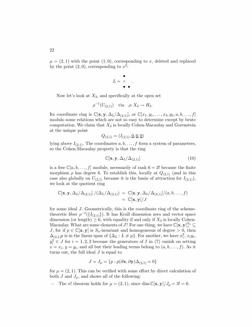
µ = (2, 1) with the point (1, 0), corresponding to x, deleted and replacedby the point (2, 0), corresponding to x2:

L =•◦• •

.

Now let’s look at X3, and specifically at the open set

ρ−1(U(2,1)) via ρ:X3 → H3.

Its coordinate ring is C[x, y,∆L/∆(2,1)], or C[x1, y1, . . . , x3, y3, a, b, . . . , f ]modulo some relations which are not so easy to determine except by brutecomputation. We claim that X3 is locally Cohen-Macaulay and Gorensteinat the unique point

Q(2,1) = (I(2,1), 0, 0, 0)

lying above I(2,1). The coordinates a, b, . . . , f form a system of parameters,so the Cohen-Macaulay property is that the ring

C[x, y,∆L/∆(2,1)] (10)

is a free C[a, b, . . . , f ] module, necessarily of rank 6 = 3! because the finitemorphism ρ has degree 6. To establish this, locally at Q(2,1) (and in thiscase also globally on U(2,1) because it is the basin of attraction for I(2,1)),we look at the quotient ring

C[x, y,∆L/∆(2,1)] /(∆L/∆(2,1)) = C[x, y,∆L/∆(2,1)]/(a, b, . . . , f)= C[x, y]/J

for some ideal J. Geometrically, this is the coordinate ring of the scheme-theoretic fiber ρ−1({I(2,1)}). It has Krull dimension zero and vector spacedimension (or length) ≥ 6, with equality if and only if X3 is locally Cohen-Macaulay. What are some elements of J? For one thing, we have C[x, y]Sn

+ ⊆J, for if p ∈ C[x, y] is Sn-invariant and homogeneous of degree > 0, then∆(2,1)p is in the linear span of {∆L : L 6= µ}. For another, we have x2

i , xiyi,y2i ∈ J for i = 1, 2, 3 because the generators of I in (7) vanish on settingx = xi, y = yi, and all but their leading terms belong to (a, b, . . . , f). As itturns out, the full ideal J is equal to

J = Jµ = {p : p(∂x, ∂y)∆(2,1) = 0}for µ = (2, 1). This can be verified with some effort by direct calculation ofboth J and Jµ, and shows all of the following:

− The n! theorem holds for µ = (2, 1), since dimC[x, y]/Jµ = 3! = 6.


− X3 is locally Cohen-Macaulay at Q(2,1).− X3 is Gorenstein at Q(2,1). The reason for this is that C[x, y]/Jµ is a

Gorenstein Artin graded algebra. In fact a graded Artin algebra C[x]/Iis Gorenstein if and only if I is the annihilating ideal of a Macaulayinverse system generated by one element, which is the case for Jµ.Since C[x, y]/J is the quotient of our Cohen-Macaulay ring in (10)by a parameter ideal, the Gorenstein property of the latter ring isequivalent to that of C[x, y]/J.

3.2. THE IDEAL SHEAF OF Xn

Our next order of business is to describe Xn as a closed subvariety ofHn × C2n by specifying its ideal sheaf, that is the subsheaf of OHn×C2n

consisting of regular functions that vanish onXn. To do this we first observethat if (I, P1, . . . , Pn) is a point of Xn, then each Pi belongs to V (I), so(I, Pi) is a point of the universal family F . In other words, Xn is a subsetof the n-fold fiber product

Fn/Hn = {(I, P1, . . . , Pn) : Pi ∈ V (I) for all i} ⊆ Hn × C2n.

Now we will describe the ideal sheaf of Xn as a subsheaf of the sheaf ofregular functions on Fn/Hn. More precisely, we will describe its pushdownto Hn. We denote the projection of F onto Hn by π, as before, and (abusingnotation slightly) we denote by ρ the projection onto Hn of Hn × C2n,or of its subschemes Xn or Fn/Hn. The projections π and ρ are affine,meaning that the inverse image of any affine open subset U ⊆ Hn is againaffine. Hence B = π∗OF contains full information about the sheaf of regularfunctions OF , and the same goes for ρ∗OFn/Hn

and ρ∗OXn . We have

B⊗n = ρ∗OFn/Hn

and we defineP = B⊗n/J = ρ∗OXn .

Our problem is to determine the sheaf of ideals J in the sheaf of OHn-algebras B⊗n. This problem is solved by the following result.

PROPOSITION 3.1. Let

φ:B⊗n → (B⊗n)∗ ⊗ ∧nB

be the homomorphism of vector bundles (or of their sheaves of sections)induced by the pairing

B⊗n ⊗B⊗n → ∧nB

24

which is multiplication in B⊗n followed by alternation:B⊗n → ∧nB. Thenthe ideal sheaf J of Xn is the kernel of φ:

J = ker φ ; P ∼= imφ.

Proof. LetΘεf =

∑w∈Sn

ε(w) wf (11)

be the alternation operator. By definition, a section g of B⊗n belongs tokerφ iff Θε(gs) = 0 for all s. Note that the regular function on (an open setin) Fn/Hn represented by any alternating section of B⊗n must vanish atevery point (I, P1, . . . , Pn) such that Pi = Pj for some i 6= j. Furthermore,Fn/Hn is the union of the locus V consisting of such points, and Xn.Suppose g belongs to J . Then so does Θε(gs), so the latter vanishes onboth V and Xn. Therefore it vanishes identically as a section of ∧nB, andg belongs to ker φ. Conversely, suppose g does not belong to J , so g doesnot vanish identically on Xn. We can find a point x = (I, P1, . . . , Pn) inXn with all Pi distinct and g(x) 6= 0, since the generic locus is dense inXn. Multiplying g by a suitable s, we can arrange that gs(wx) = 0 for all1 6= w ∈ Sn, but gs(x) 6= 0. Then Θε(gs)(x) 6= 0, so g 6∈ kerφ. 2

3.3. THE ANNIHILATING IDEAL OF ∆µ

The significance of Proposition 3.1 is that its implicit description of the idealsheaf J closely parallels a similar implicit description of the annihilatingideal Jµ ⊆ C[x, y] for the Macaulay inverse system Dµ generated by ∆µ.

PROPOSITION 3.2. Let

Jµ = {p ∈ C[x, y] : p(∂x, ∂y)∆µ = 0}.Then p belongs to Jµ if and only if the coefficient of ∆µ in Θε(ps) is zero,for all s ∈ C[x, y].

Here Θε is the alternation operator in (11). It makes sense to speak ofthe coefficient of ∆µ in Θε(ps), because the polynomials ∆M form a basisof C[x, y].

Proof. The coefficient Θε(ps)|∆µ is, apart from a fixed scalar factor,just the constant term of s(∂x, ∂y)p(∂x, ∂y)∆µ. By Taylor’s theorem, thisvanishes for all s if and only if p(∂x, ∂y)∆µ = 0. 2


We can reformulate the above proposition in the following suggestiveway. Recall that Iµ ∈ Hn denotes the ideal spanned by all monomials notin the diagram of µ. We see immediately that in the ring

B⊗n(Iµ) = C[x, y]/(Iµ(x1, y1) + · · ·+ Iµ(xn, yn)),

the image of ∆L(x, y) vanishes for all L 6= µ, while the image of ∆µ spansthe one-dimensional space ∧nB(Iµ). Hence the composite map

C[x, y] → B⊗n(Iµ) → ∧nB(Iµ) ∼= C

is in effect given by Θε(−)|∆µ . This yields:

COROLLARY 3.3. The ideal Jµ is the kernel of the composite map

C[x, y] → B⊗n(Iµ) →φ(Iµ)

B⊗n(Iµ)∗ ⊗ ∧nB(Iµ).

It might appear that Proposition 3.1 and Corollary 3.3 immediatelyimply that Jµ is (modulo Iµ(x1, y1) + · · ·+ Iµ(xn, yn)) the fiber of J andthat C[x, y]/Jµ is the fiber of P at the point Iµ ∈ Hn. In reality, the matteris not quite so simple. For one thing, we don’t know yet that P and J arelocally free, i.e., that they are the sheaves of sections of vector bundles.Absent this, their “fibers” at Iµ are not necessarily what intuition wouldsuggest. Even if we assume that they are locally free, if we carefully examinethe passage from sheaves of sections to fibers, the only conclusion we candraw immediately is that Jµ contains the fiber J (Iµ). Nevertheless, thefollowing facts do hold:

− P (and hence also J ) is locally free if and only if Xn is Cohen-Macaulay. This follows because Hn is non-singular and ρ:Xn → Hn isfinite; in this situation, the local freeness of P = ρ∗OXn is essentiallythe definition of the Cohen-Macaulay property.

− Generically, P is locally free of rank n!, because the map ρ is generi-cally n!-to-one. When I = I(S), there are n! choices for the orderingP1, . . . , Pn of the distinct points of S.

− It follows that every fiber of the linear map φ has rank at most n!, andthat coker φ, P and J are all locally free in a neighborhood of I ∈ Hn

if and only if φ(I) has rank n!.− The ring C[x, y]/Jµ is Gorenstein. More generally, a graded Artin al-

gebra C[x]/J is Gorenstein if and only if J is the annihilating ideal ofa Macaulay inverse system generated by one element [6]. If you like,you may take this as the definition of Gorenstein for a graded Artinalgebra; then a general graded algebra is Gorenstein if it is Cohen-Macaulay and its quotient by any (equivalently every) homogeneousparameter ideal is Gorenstein Artin. By the way, Artin means Krulldimension zero, or finite dimension as a vector space.

26

Using these facts, one can deduce from Proposition 3.1 and Corollary 3.3the following theorem.

THEOREM 3.4. Let Qµ = (Iµ, 0, . . . , 0) be the unique point of Xn lyingover Iµ ∈ Hn. The following are equivalent:

(1) Xn is locally Cohen-Macaulay and Gorenstein at Qµ;(2) the n! theorem (Theorem 1.1) holds for the partition µ.

When these conditions hold, moreover, Jµ is the ideal of the scheme-theoreticfiber ρ−1(Iµ) ⊆ Xµ, that is, we have C[x, y]/Jµ

∼= P (Iµ).

Proof. First assume (1) holds. Then P and J are locally free, and Jµ

contains J (Iµ). Moreover, P (Iµ) = B⊗n(Iµ)/J (Iµ) is a Gorenstein Artinring on which Sn acts by the regular representation. Its socle, or uniqueminimal ideal, is one-dimensional, so Sn must necessarily act on it by thesign representation. If Jµ is not equal to J (Iµ), then Jµ must contain the so-cle, and hence C[x, y]/Jµ does not contain a copy of the sign representationof Sn. In particular, we must have ∆µ ∈ Jµ, which is absurd.

Conversely, assume (2) holds. Then φ(Iµ) has rank n!, so Xn is locallyCohen-Macaulay at Iµ. Furthermore, J (Iµ) = Jµ, so P (Iµ) ∼= C[x, y]/Jµ isGorenstein, which implies Xn is Gorenstein at Iµ.

We have now tied together two of our seemingly unrelated theoremsfrom Lecture 1, namely, the n! theorem, and the geometric theorem thatXn is Gorenstein. In fact, we have shown that the latter theorem impliesthe n! theorem.

3.4. THE NESTED HILBERT SCHEME

For ideals In−1 ∈ Hn−1, In ∈ Hn, the condition that In ⊆ In−1 is a closedcondition on Hn−1 ×Hn, i.e., it is defined by polynomial equations in localcoordinates (much like those for the corresponding condition on a productof Grassmann varieties). Hence we can define the nested Hilbert scheme

Hn−1,n ⊆ {(In−1, In) : In ⊆ In−1} ⊆ Hn−1 ×Hn

as a closed subscheme. Geometrically, it parametrizes pairs of finite sub-schemes Sn−1 ⊆ Sn ⊆ C2, of lengths n − 1 and n. There is a remarkableextension of Fogarty’s theorem to the nested case.

THEOREM 3.5. (Tikhomirov, unpublished; see [4] for proof). The nestedHilbert scheme Hn−1,n is non-singular and irreducible, of dimension 2n.


One can define more general nested Hilbert schemes parametrizing flagsof subschemes of various lengths. Cheah [4] has shown that of these onlyHn

and Hn−1,n are non-singular, apart from some small exceptions like H1,2,3.We will prove Theorem 1.7, the Gorenstein property ofXn, by induction

on n, using the nested Hilbert scheme to provide the geometric link betweenXn−1 and Xn. For this we need to introduce the nested isospectral Hilbertscheme Xn−1,n. But first we must discuss Hn−1,n a little more. Given apair In ⊆ In−1 in Hn−1,n, there is a unique distinguished point P ∈ V (In)such that the length of (R/In)P is exceeds the length of (R/In−1)P by1. In terms of the Chow morphisms, if σn−1(In−1) = JP1, . . . , Pn−1K, thenσn(In) = JP1, . . . , Pn−1, P K, where P is the distinguished point. Anotherway to look at this is that the R-module In−1/In has length 1, hence isisomorphic to R/m = C[x, y]/(x− xn, y − yn) for some maximal ideal m.Then (xn, yn) are the coordinates of P . We get a Chow morphism

σn−1,n:Hn−1,n → Sn−1C2 × C2

defined byσn−1,n(In−1, In) = (σn−1(In−1), P ).

Both maps Hn−1,n → Sn−1C2 and Hn−1,n → SnC2 induced by the Chowmorphisms σn−1 and σn composed with the projections on Hn−1 and Hn

factor through σn−1,n.

DEFINITION 3.6. The nested isospectral Hilbert scheme Xn−1,n is thereduced fiber product

Xn−1,n −−−→ C2ny yHn−1,n −−−→ Sn−1C2 × C2.

(12)

In other words, the points of Xn−1,n are tuples (In−1, In, P1, . . . , Pn),where In ⊆ In−1, σn(In) = JP1, . . . , PnK, and Pn is the distinguished point.Note that the reduced fiber product Y in the diagram

Y −−−→ Hn−1,ny yXn−1 −−−→ Hn−1

(13)

can be identified with the set of tuples (In−1, In, P1, . . . , Pn−1) such thatIn ⊆ In−1 and σn−1(In−1) = JP1, . . . , Pn−1K. Then Xn−1,n is the graph ofthe morphism Y → C2 sending (In−1, In, P1, . . . , Pn−1) to its distinguished

28

point P = Pn. Thus the above fiber product Y provides an alternativedescription of Xn−1,n.

We can now indicate roughly how the proof of Theorem 1.7 goes. Weconsider the larger diagram

Y = Xn−1,ng−−−→ Xn

↘yy Hn−1,n −→ Hny

Xn−1 −→ Hn−1

(14)

We are to prove that Xn is Gorenstein, and we will assume the result forXn−1 by induction. Then the bottom arrow in (14) is flat with Gorensteinfibers, since it is finite and Hn−1 is non-singular. Hence the same holds forthe diagonal arrow if we take Y to be the scheme-theoretic fiber product.Since Hn−1,n is non-singular, the scheme-theoretic fiber product is againGorenstein. It is generically reduced, hence reduced, hence equal toXn−1,n.This shows that Xn−1,n is Gorenstein. The morphism g : Xn−1,n → Xn

given by the top arrow in (14) is projective and birational, allowingXn−1,n

to play the role of a partial desingularization of Xn. To complete the proofwe will use duality for the morphism g to deduce that Xn is Gorenstein, asdesired. In order to do this we will need the identity

Rg∗OXn−1,n = OXn

for the derived functor Rg∗ of the sheaf pushforward functor g∗. At the endof the day, to establish this identity we will need know something moreabout Xn than what follows merely from the inductive set-up. What thatsomething is and how to prove it will be taken up in the next lecture.

4. The main theorem and the polygraph theorem

4.1. MAIN THEOREM

We start by adding some details to the outline of the proof of Theorem 1.7given at the end of the last lecture. We want to prove that Xn is Gorensteinby induction on n, but we need to refine the induction hypothesis a bit.

The Proj construction gives rise to a line bundle denoted O(1) on anyX = ProjS, such that the elements of S1 represent global sections of O(1).The k-th tensor power of O(1) is denoted O(k); if k is negative, this meansthe (−k)-th tensor power of the dual O(−1) = O(1)∗. In the case of Hn


and Xn, it follows from the proof of Theorem 2.1 that O(1) = ∧nB. EveryGorenstein scheme X possesses a canonical line bundle (more on this below)which in the case of a non-singular scheme is the usual canonical line bundle,i.e., the sheaf of exterior differential d-forms, where d = dimX . What wewill prove by induction is that

Xn is Gorenstein, with canonical line bundle equal to O(−1).

As explained in the last lecture, we can deduce from the inductionhypothesis for n − 1 that Xn−1,n, is Gorenstein. In fact we can do a littlebetter. The relative canonical line bundles for the bottom arrow and thediagonal arrow in (14) are the same. On Hn−1,n and Xn−1,n, we writeO(k, l) for the tensor product of the pullback of O(k) from Hn−1 with thepullback of O(l) from Hn. By an explicit calculation in [17], the canonicalsheaf of Hn−1 is O (this was well-known) and that of Hn−1,n is O(1,−1)(this is new). By the induction hypothesis and the calculation for Hn−1,the relative canonical sheaf for the bottom and diagonal arrows in (14)is O(−1, 0). Hence by the calculation for Hn−1,n the canonical sheaf onXn−1,n is O(0,−1), that is, the pullback g∗OXn(−1) of O(−1) from Xn.

The key to the proof is to show that for the projection g:Xn−1,n → Xn

we haveRg∗OXn−1,n = OXn .

Here Rg∗ is the derived functor of the pushforward g∗. For present purposes,everything you need to know about derived functors and derived categoriescan be summed up as follows.

− On every scheme X of finite type over a field there is a complex ofsheaves ωX , which is a dualizing object in the derived category. Thismeans that the derived functor DX = RHom(−, ωX) satisfies DX ◦DX = id. Although a dualizing object is not unique, there is a canonicalpreferred choice (up to isomorphism in the derived category).

− IfX is Cohen-Macaulay and d-dimensional, then ωX reduces to a singlesheaf concentrated in degree −d. If X is also Gorenstein, that sheaf isthe canonical line bundle on X . The converse statements also hold.

− Duality theorem: if g: Y → X is a proper (e.g., projective) morphism,then the derived functor Rg∗ commutes with duality, i.e., DX ◦Rg∗ =Rg∗ ◦ DY .

− Projection formula: if L is a locally free sheaf on X , then Rg∗(A ⊗g∗L) = (Rg∗A) ⊗ L.

Now let’s grant for a moment that Rg∗OXn−1,n = OXn . We have establishedthat Xn−1,n is Gorenstein with canonical sheaf g∗OXn(−1), and hence itsdualizing complex is this sheaf, concentrated in degree −2n. The morphism

30

g is projective. On the one hand, using the projection formula with A =OXn−1,n and L = OXn(−1), we deduce

Rg∗g∗OXn(−1) = OXn(−1).

On the other hand, using the duality theorem, we deduce

Rg∗ωXn−1,n = ωXn .

Together, these two identites show that ωXn is the sheaf OXn(−1) concen-trated in degree −2n. Hence Xn is Gorenstein with canonical sheaf O(−1),which is what we wanted to prove.

How do we show that Rg∗OXn−1,n = OXn? First of all, this is a localquestion on the target Xn of g. On the locus where P1, . . . , Pn are not allequal, Xn is locally isomorphic to a product Xk ×Xl for some k, l < n, andg is locally isomorphic to g′:Xk×Xl−1,l → Xk ×Xl. This is intuitively easyto understand and not hard to prove, so I refer you to [17] for the details.We can assume as part of the induction that Rg′∗O = O, so we only haveto worry about the situation in the neighborhood of points of Xn whereP1, . . . , Pn all coincide. In particular, we only have to worry about whathappens where y1 − y2, y2 − y3, . . . , yn−1 − yn all vanish.

Now there is a standard technique for dealing with this situation usinglocal cohomology. Again I refer you to [17] for technical details, but theupshot is that to extend the identity Rg∗OXn−1,n = OXn from the comple-ment of V (y1 − y2, . . . , yn−1 − yn) to the whole of Xn and Xn−1,n we onlyneed to establish three facts:

(a) The sequence y1 − y2, . . . , yn−1 − yn is a regular sequence in the localring of OXn at every point x ∈ V (y1 − y2, . . . , yn−1 − yn),

(b) The same holds in OXn−1,n , and(c) The fibers of g have dimension less than n− 2.

To complete your confusion, we define another morphism

α:Hn−1,n → F (15)

sending (In−1, In) to (In, P ). Since the distinguished point can be any pointof In (for some choice of In−1), the image of α is indeed F . Generically,when In = I(S), we must have In−1 = I(S \ {P}), so the fiber of α over(I(S), P ) has just one point. Thus α is birational (it’s also projective). Thefibers of g are actually fibers of α, as you will see if you understand theremarks following Definition 3.6. The fiber of α over a point (I, P ) is theprojective space P(A) where A is the socle of the local ring (R/I)P , thatis, the annihilator of the maximal ideal. Its dimension must be maximizedat a monomial ideal. Hence the maximum fiber dimension is one less than


the maximum number of corners of the diagram of a partition µ of n. Forn ≥ 4, the number of corners of µ is always less than n − 1, so fact (c)holds.

For fact (b), we already know thatXn−1,n is Cohen-Macaulay, so we onlyhave to show that the locus V (y1−y2, . . . , yn−1−yn) has codimension n−1 inXn−1,n. Then it is a local complete intersection, and, by the general theoryof Cohen-Macaulay rings, the generators of its ideal form a regular sequence.The required dimension estimate follows from the cell decomposition ofHn−1,n in [4].

The heart of the matter is fact (a). It is true that V (y1−y2, . . . , yn−1−yn)has codimension n− 1 in Xn, but this information is useless since we don’tknow in advance that Xn is Cohen-Macaulay. What we need is the followinglemma.

LEMMA 4.1. The map Xn → Cn = Spec C[y], given by the compositeof the blowup map Xn → C2n with the projection C2n → Cn on the ycoordinates, is flat.

Granting this lemma, the proof is otherwise complete, except that weonly have fact (c) for n ≥ 4. For n = 1, 2, 3, we need to verify the inductionhypothesis directly. The action of (C∗)2 on C2 as the group of 2×2 diagonalmatrices induces an action of (C∗)2 on Xn in which every point has someQµ in the closure of its orbit. Using this fact, we can reduce the problemof showing that Xn is Gorenstein to the local problem at the distinguishedpoints Qµ. Then, using Theorem 3.4, we need only verify the n! theoremfor each ∆µ with |µ| ≤ 3. This is an easy computation which I invite you tocarry out by hand. The only case you really have to check is µ = (2, 1), sincethe others are classical Vandermonde determinants in one set of variables.

The multiplication and alternation pairing B⊗n ⊗B⊗n → ∧nB = O(1)in Proposition 3.1 induces a pairing P ⊗ P → O(1). Once we know Xn isGorenstein, P becomes a vector bundle and the induced pairing is perfecton every fiber. By the duality theorem for the finite morphism ρ:Xn → Hn

this implies that ωXn = O(−1). So we have verified the full inductionhypothesis, as we stated it, for n = 1, 2, 3.

Technically, the identity Rg∗OXn−1,n = OXn is part of the inductionhypothesis too. For n = 1, 2, the morphism g is an isomorphism, and thisidentity is trivial. For n = 3, g is everywhere locally an isomorphism, exceptover the locus Z consisting of non-curvilinear triple points. But in thiscase, we know that both X2,3 and X3 are Cohen-Macaulay, and we canfind a sequence z1, z2, z3 of global functions, regular on both X2,3 and X3

and vanishing on Z. Using this we can verify that Rg∗OX2,3 = OX3 by astandard local cohomology argument, like the one alluded to earlier in ourdiscussion of the induction step.

32

4.2. THE POLYGRAPH THEOREM ENTERS THE SCENE

Recall from Lecture 1 the definition of the polygraph Z(n, l) ⊆ C2n+2l andthe theorem (whose proof we will discuss later on) that its coordinate ringis a free C[y]-module, where x, y, a,b are the coordinates on C2n+2l. Wewill now show how Lemma 4.1 follows from the polygraph theorem and theconstruction of Xn as a blowup. Recall specifically that

Xn = ProjC[x, y][tJ] = Proj⊕

d

Jd,

where J = C[x, y]A is the ideal generated by the alternating polynomials.To establish Lemma 4.1 it suffices to prove the following proposition.

PROPOSITION 4.2. The ideal Jd is a free C[y]-module for all d.

Proof. Set l = dn, and let Z(n, l) ⊆ C2n+2l be the polygraph. Recallthat this is the union of the subspaces

Wf = V (ai − xf(i), bi − yf(i) : 1 ≤ i ≤ l),

for all f : {1, . . . , l} → {1, . . . , n}. Let G = Sdn be the Cartesian product

of d copies of the symmetric group Sn, acting on C2n+2l by permuting thefactors in C2l = (C2)dn in d consecutive blocks of length n. In other wordseach w ∈ G fixes the coordinates x, y on C2n, and for each k = 0, . . . , d− 1permutes the coordinate pairs akn+1, bkn+1 through akn+n, bkn+n amongthemselves.

Let R(n, l) = C[x, y,a,b]/I(n, l) be the coordinate ring of Z(n, l). ByTheorem 1.8, R(n, l) is a free C[y]-module. By the symmetry of its defi-nition, I(n, l) is a G-invariant ideal, so G acts on R(n, l). We claim thatJd is isomorphic as a C[x, y]-module to the space R(n, l)ε of G-alternatingelements of R(n, l). Each x-degree homogeneous component of R(n, l) isa finitely generated y-graded free C[y]-module. Since R(n, l)ε is a gradeddirect summand of R(n, l), it is a free C[y]-module, so the claim proves theProposition.

Define a function f0 by f0(kn + i) = i for all 0 ≤ k < d, 1 ≤ i ≤ n.Restriction of regular functions from Z(n, l) to its component subspaceWf0 is given by the C[x, y]-algebra homomorphism ψ : R(n, l) → C[x, y]mapping akn+i, bkn+i to xi, yi. Observe that ψ maps R(n, l)ε surjectivelyonto C[x, y]Ad = Jd. In fact, R(n, l)ε is the C[x, y]-submodule of R(n, l)generated by products of the form

∆M1(a1, b1, . . . , an, bn) · · ·∆Md(a(d−1)n+1, b(d−1)n+1, . . . , adn, bdn).


Let p be an arbitrary element of R(n, l)ε. Since p is G-alternating, pvanishes on Wf if f(kn + i) = f(kn + j) for some 0 ≤ k < d and some1 ≤ i < j ≤ n. Thus the regular function defined by p on Z(n, l) isdetermined by its restriction to those components Wf such that for eachk, the sequence f(kn + 1), . . . , f(kn + n) is a permutation of {1, . . . , n}.Moreover, for every such f there is an element w ∈ G carrying Wf ontoWf0. Hence p is determined by its restriction to Wf0. This shows that pvanishes on Z(n, l) if ψ(p) = 0, that is, the kernel of ψ:R(n, l)ε → Jd iszero. Hence ψ is injective as well surjective, so it’s an isomorphism. 2

At this point, everything is left hanging solely on the proof of the poly-graph theorem. Before we turn to the discussion of that proof, I want tomake a few more remarks on the geometric topics.

The first remark is that the polygraph has a direct geometric relevance tothe Hilbert scheme picture, which is somewhat obscured by its roundaboutentrance via Lemma 4.1 and Proposition 4.2. To see this, consider theuniversal family F/Xn = F ×Hn Xn pulled back to Xn, and its l-th fiberpower

F l/Xn = {(I, P1, . . . , Pn, Q1, . . . , Ql) : Qi ∈ V (I) for all i}.Since σ(I) = JP1, . . . , PnK the condition Qi ∈ V (I) is equivalent to Qi ∈{P1, . . . , Pn}. It follows immediately that the projection on C2n+2l of F l/Xn

⊆ Hn × C2n+2l is nothing other than the polygraph Z(n, l). In particular,every regular function on Z(n, l) can be composed with this projection toyield a global regular function on F l/Xn. The latter is the same thingas a global section of B⊗l over Xn (abusing notation, we write B forwhat is really ρ∗B). So we have a canonical, geometrically defined ringhomomorphism

R(n, l) → H0(Xn, B⊗l).

Later we will see that this homomorphism is an isomorphism, and what’smore, the higher cohomology modules H i(Xn, B

⊗l) vanish for i > 0. If wegrant in advance that Xn is Cohen-Macaulay, and observe that the locusV (y) is a complete intersection in Xn, these facts in turn imply that R(n, l)is a free C[y]-module. So, conceptually, the right idea is that R(n, l) is freebecause Xn is Cohen-Macaulay and the tensor powers of B enjoy a strongcohomology vanishing theorem on Xn. For now, however, we are obliged towork backwards and prove that R(n, l) is free by getting our hands dirty.

The second remark concerns the ideal J and its powers. Any alternatingpolynomial must obviously vanish at a point of C2n where xi = xj andyi = yj, for i 6= j. Thus we have obvious inclusions

J ⊆⋂i<j

(xi − xj, yi − yj),

34

and consequentlyJd ⊆

⋂i<j

(xi − xj, yi − yj)d.

It is a consequence of Proposition 4.2 that equality holds here:

PROPOSITION 4.3. For all n and d, we have

Jd =⋂i<j

(xi − xj, yi − yj)d. (16)

Proof. We first consider the situation locally at a point where the yi arenot all equal. With a little work, it can be shown that (16) reduces at sucha point to the same equation for smaller values of n. Thus we can assumeby induction that (16) holds locally on U = C2n \V (y1−y2, . . . , yn−1−yn).Since Jd is a free C[y]-module, the ring C[x, y]/Jd has depth at least n−1 asa C[y]-module. This implies that V (Jd) is scheme-theoretically equal to theclosure of its intersection with any open set of the form C2n \ V (I), whereI is generated by at least two independent linear forms in y. In particular,for n ≥ 3, V (Jd) is the closure of its intersection with U , establishing (16).For n = 1, 2, the result is trivial. 2

Proposition 4.3 and Theorem 2.1 justify the assertion that Hn and Xn

are the blowups of SnC2 and C2n, respectively, along the reduced union ofpairwise diagonals. See the remarks following Theorem 2.1. Proposition 4.3also implies that the ideals Jd are integrally closed, and hence the Reesealgebra T = C[x, y][tJ] is an integrally closed domain. By definition, thisshows that Xn is arithmetically normal in its realization as ProjT . Inparticular, Xn is normal, i.e., its local ring at every point is integrallyclosed.

We conjecture that Theorem 1.8 holds for the polygraph Z(n, l) ⊆Ckn+kl over E = Ck for any k, with freeness over the polynomial ringC[z] in any one set of n coordinates on Ckn. If true, this would imply thatProposition 4.2 and Proposition 4.3 hold in more than two sets of variablesx, y, . . . , z, with essentially the same proof. At present we cannot prove anyof these results for k > 2, not even the “intuitively obvious” case d = 1of Proposition 4.3. Indeed we cannot prove these results for k = 2 withoutrecourse to the polygraph theorem. For k = 1, by contrast, they are easyand well-known: the ideal J is generated by the Vandermonde determinant∆(x), and the intersection of ideals in (16) is equal to the their product.


4.3. THE POLYGRAPH BASIS

Rather than go over the proof of the polygraph theorem as presented in[17], what I would like to do is reveal the secret behind it. The secret is analgorithm for producing the elements of a free module basis of R(n, l), interms of combinatorial indexing data. The indexing data are pairs

e = (e1, . . . , en) ∈ Nn, f : [l] → [n].

Here and below we use the abbreviation [k] = {1, . . . , k}. Recall that R(n, l)is a quotient of a polynomial ring

R(n, l) = C[x, y, a,b]/I(n, l),

so our basis elements will be represented by polynomials

p[e, f ] ∈ C[x, y, a,b].

As R(n, l) is doubly graded by degree in the x, a variables (“x-degree”)and the y,b variables (“y-degree”), our elements p[e, f ] will be doublyhomogeneous. They will also satisfy certain important vanishing conditions.To describe the conditions, we introduce loci Y (m, r, k) ⊆ Z(n, l) definedby

Y (m, r, k) =⋃V (xT ) ∩Wf : |T ∩ [r] \ f([k])| ≥ m.

Here T is a subset of [n] and V (xT ) is shorthand for V (xj : j ∈ T ). Recallthat Wf is the component of the polygraph Z(n, l) on which ai = xf(i),bi = yf(i) for all i ∈ [l]. Thus, informally, Y (m, r, k) is the locus on which atleast m of the first r coordinates xj vanish, coordinates in f([k]) excluded.The ideal of Y (m, r, k) is called I(m, r, k). The basis elements p[e, f ] willsatisfy

− degx p[e, f ] = |e| = e1 + · · ·+ en,− degy p[e, f ] = i(e, f), defined below,− p[e, f ] ∈ I(m, r, k) iff |(supp e)c ∩ [r] \ f([k])| < m, and these elements

span I(m, r, k) as a C[y]-module.

Here supp e is the set of indices j with ej 6= 0, and (supp e)c is its com-plement. The last condition implies that the ideals I(m, r, k) generate adistributive sublattice of the lattice of ideals inR(n, l), all of whose membersare spanned by subsets of the basis {p[e, f ]}. It follows that the coordinatering of any intersection of unions of the loci Y (m, r, k) is again a freeC[y]-module (and also that every such intersection is scheme-theoreticallyreduced).

Let’s check that at least in a certain weak sense, the numbers work out.Any free C[y]-module basis of R(n, l) must also be a C(y)-vector space basis

36

of C(y)⊗ R(n, l). In C(y)⊗ R(n, l) we can form for each f the rationalfunction

1f =∏

i

∏j 6=f(i)

bi − yj

yf(i) − yj,

which is identically 1 on Wf and vanishes on all other components Wg (itis undefined where Wf and Wg intersect). The set of all elements

xe1f

is a C(y)-basis of C(y)⊗ R(n, l). In this basis, it is not hard to see thatC(y)⊗ I(m, r, k) is spanned by the elements

xe1f : |(supp e)c ∩ [r] \ f([k])| < m.

The reason is that if |T ∩ [r] \ f([k])| ≥ m and e, f are as above, then(supp e)c cannot contain T , that is, (supp e) ∩ T is non-empty, so xe mustvanish on V (xT ). This shows that in each x-degree, we have specified theright number of elements p[e, f ] to belong in I(m, r, k).

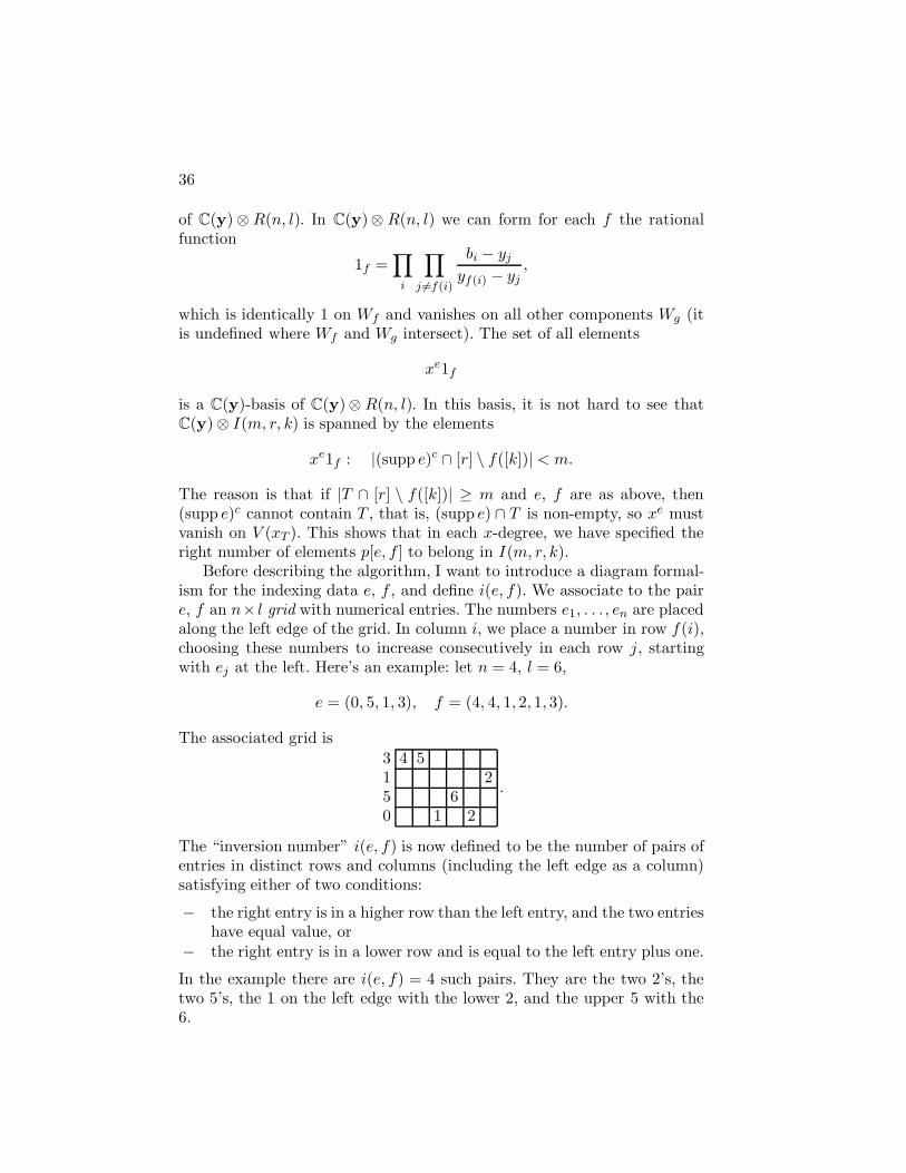
Before describing the algorithm, I want to introduce a diagram formal-ism for the indexing data e, f , and define i(e, f). We associate to the paire, f an n× l grid with numerical entries. The numbers e1, . . . , en are placedalong the left edge of the grid. In column i, we place a number in row f(i),choosing these numbers to increase consecutively in each row j, startingwith ej at the left. Here’s an example: let n = 4, l = 6,

e = (0, 5, 1, 3), f = (4, 4, 1, 2, 1, 3).

The associated grid is3 4 51 25 60 1 2

.

The “inversion number” i(e, f) is now defined to be the number of pairs ofentries in distinct rows and columns (including the left edge as a column)satisfying either of two conditions:

− the right entry is in a higher row than the left entry, and the two entrieshave equal value, or

− the right entry is in a lower row and is equal to the left entry plus one.

In the example there are i(e, f) = 4 such pairs. They are the two 2’s, thetwo 5’s, the 1 on the left edge with the lower 2, and the upper 5 with the6.


If we define the generating function

An,l(q, t) =1

(1− q)n

∑e,f

t|e|qi(e,f),

it follows that the Hilbert series of R(n, l) as a doubly graded algebra isgiven by ∑

r,s

trqs dimR(n, l)r,s = An,l(q, t).

In particular we must have An,l(q, t) = An,l(t, q), a fact which is ratheramazing when considered in light of the combinatorial definition. Later wewill see that there is an explicit formula for An,l(q, t) in terms of operatorson Macdonald polynomials.

The quantity i(e, f) can be computed by a combinatorial recurrence.The key to this is to observe that i(e, f) remains invariant if we “cycle” thegrid by moving the bottom row to the top, and subtracting one from eachentry of that row. Doing this only gives a new legal grid if e1 > 0, but thereare modifications that work when e1 = 0. Altogether there are three cases.Once and for all we fix the cyclic permutation

θ = (1 2 . . . n).

In terms of θ the result of cycling the grid for e, f is the grid for e′ =θ−1e− (0, . . . , 0, 1), f ′ = θ−1f .Case I: e1 = 0 and 1 6∈ f([l]), i.e. the only entry in the bottow row is azero at the left edge. The bottom row contributes nothing to i(e, f), soi(e, f) = i(e′, f ′), where e′ = (θ−1e)|[n−1], f ′ = θ−1f . Note that e′ ∈ Nn−1

and f ′ has image in [n − 1]. The grid of e′, f ′ is gotten by deleting thebottom row from the grid of e, f .Case II: e1 = 0 and t = min f−1({1}), i.e. there is a 1 in the bottom rowof the grid, in column t. Then

i(e, f) = i(e′, f ′) +m,

where e′ = θ−1e, f ′ = θ−1f |L, L = [l] \ {t}, and m = |(supp e)c \ f−1([t])|.In other words, m is the number of rows in the grid with a zero at the leftedge, and no entry in columns 1, . . . , t (in particular, the bottom row doesnot count). The grid of e′, f ′ is gotten by deleting column t from the grid ofe, f and cycling without diminishing e1. Note however that any remainingentries in the bottom row will get diminished as a result of deleting columnt.Case III: e1 > 0. Then i(e, f) = i(e′, f ′), where e′ = θ−1e − (0, . . . , 0, 1),f ′ = θ−1f . The grid of e′, f ′ is the result of cycling the grid of e, f ,diminishing e1 by 1.

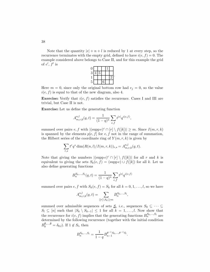
38

Note that the quantity |e| + n+ l is reduced by 1 at every step, so therecurrence terminates with the empty grid, defined to have i(e, f) = 0. Theexample considered above belongs to Case II, and for this example the gridof e′, f ′ is

0 13 4 51 25 6

.

Here m = 0, since only the original bottom row had ej = 0, so the valuei(e, f) is equal to that of the new diagram, also 4.

Exercise: Verify that i(e, f) satisfies the recurrence. Cases I and III aretrivial, but Case II is not.

Exercise: Let us define the generating function

An,lm,r,k(q, t) =

1(1 − q)n

∑e,f

t|e|qi(e,f),

summed over pairs e, f with |(supp e)c ∩ [r] \ f([k])| ≥ m. Since I(m, r, k)is spanned by the elements p[e, f ] for e, f not in the range of summation,the Hilbert series of the coordinate ring of Y (m, r, k) is given by∑

r,s

trqs dim(R(n, l)/I(m, r, k))r,s = An,lm,r,k(q, t).

Note that giving the numbers |(supp e)c ∩ [r] \ f([k])| for all r and k isequivalent to giving the sets Sk(e, f) = (supp e) ∪ f([k]) for all k. Let usalso define generating functions

BS0,...,Sln (q, t) =

1(1 − q)n

∑e,f

t|e|qi(e,f)

summed over pairs e, f with Sk(e, f) = Sk for all k = 0, 1, . . . , l, so we have

An,lm,r,k(q, t) =

∑|[r]\Sk|≥m

BS0,...,Sln ,

summed over admissible sequences of sets S, i.e., sequences S0 ⊆ · · · ⊆Sl ⊆ [n] such that |Sk \ Sk−1| ≤ 1 for all k = 1, . . . , l. Now show thatthe recurrence for i(e, f) implies that the generating functions BS0 ,...,Sl

n aredetermined by the following recurrence (together with the initial conditionB∅,...,∅

0 = δ0,l). If 1 6∈ Sl, then

BS0,...,Sln =

11 − q

Bθ−1S0,...,θ−1Sln−1 .


If 1 ∈ St \ St−1, then

BS0 ,...,Sln = qn−|St | ∑

S′0,...,S′

l−1

BS′

0 ,...,S′l−1

n ,

summed over admissible S′ such that S ′i = θ−1Si for i < t and S ′

i ∪ {n} =θ−1Si+1 for i ≥ t (note that n ∈ θ−1Si+1 for these values of i). If 1 ∈ S0,then

BS0 ,...,Sln = t

∑S′

0,...,S′l

BS′

0,...,S′l

n ,

where S ′ is admissible and S ′i ∪ {n} = θ−1Si for all i.

5. Constructing the basis

5.1. BASIS CONSTRUCTION ALGORITHM

Recall from the last lecture that our plan is to give a basis of R(n, l) consist-ing of doubly homogeneous polynomials p[e, f ] for e ∈ Nn and f : [l] → [n]such that

− degx p[e, f ] = |e|,− degy p[e, f ] = i(e, f),− p[e, f ] ∈ I(m, r, k) ⇔ |(supp e)c ∩ [r] \ f([k])| < m,

where i(e, f) is the number of inversions in the grid diagram of (e, f), asdefined in the last lecture. Also, the elements p[e, f ] we have specified tobelong to I(m, r, k) will actually span this ideal as a C[y]-module.

We now present an algorithm to compute p[e, f ]. In places, the algo-rithm specifies that we should compute some polynomial as the uniquesolution of some linear equations over C[y]. At such points, of course, thereis something to prove. First, the solution should exist and be unique inlinear algebra over the field of rational functions C(y), and second, theresulting polynomial should belong to C[x, y, a,b] when, a priori, it mightonly belong to C(y)[x, a,b]. These things are true, but I will not attemptto justify them fully here.

You can readily imagine a possible proof of the polygraph theorem alongthese lines: (1) present the algorithm, (2) prove that it works. The approachactually taken in [17] looks quite different. There I inductively constructbases for the rings R(n, l)/I(1, 1, t) for t going from l to 0, and finallyfor R(n, l). The algorithm presented here is what you get by unravellingthe inductive construction presented in Section 4.10 of [17], and the proofthat it works is implicit in the proof of the relevant lemmas there. Afterpresenting the algorithm, I’ll say a bit below about what is going on in

40

the proof of its correctness, and why the less algorithmic approach in [17]seems to be the only workable method.

In the algorithm to compute basis elements p[e, f ] in R(n, l), we willassume that they have already been computed in R(n−1, l), in R(n, l−1),and in smaller x-degrees in R(n, l). The starting point for the recurrence isthe case l = 0. Then we have R(n, 0) = C[x, y], and the required basis is

p[e, ∅] = xe.

This also covers the case n = 0, since R(0, l) = 0 if l > 0.Given (e, f), we set

t =

0 if e1 > 0l + 1 if e1 = 0 and 1 6∈ f([l])min f−1({1}) otherwise.

The value of t is, so to speak, the position of 1 in the bottom row of thegrid, with the convention that a missing 1 is “outside” the grid, on the leftedge if e1 > 1 and on the right edge if e1 = 0. We fix

θ = (1 2 . . . n),

as before.The algorithm proceeds in two phases. In the first phase, we construct

a proto-basis, whose elements we denote q[e, f ]. In the second phase, wecorrect these to get the p[e, f ]. To compute an individual p[e, f ] we wouldfirst have to compute all the proto-basis elements q[e, f ] of the same bi-degree, so in practice we might as well compute all p[e, f ] of a given bi-degreeat once. The proto-basis construction has three cases. Comparing them withthe three cases in the recurrence for i(e, f), you will see that i(e, f) doescorrectly give the y-degree of the constructed elements.Case I: t = l + 1. In other words, e = (0, e2, . . . , en) and f maps [l] into[n] \ {1}. Note that (θ−1e)|[n−1] ∈ Nn−1 determines e and that θ−1f maps[l] into [n− 1]. In this case, set

q[e, f ] = θpn−1,l[(θ−1e)|[n−1], θ−1f ],

the right-hand side having already been computed in R(n− 1, l).Case II: 1 ≤ t ≤ l. Define

Z ′(r, t) = V (at) ∩⋃f ′Wf ′ : f ′(t) ∈ [r] \ f ′([t− 1]), (17)

a subspace arrangement contained in R(n, l) as a closed subset. Set L =[l] \ {t}, and denote by R(n, L) the ring R(n, l − 1) using a,b variables


ai, bi : i ∈ L, that is, omitting index t. It is a fact that the coordinate ringO(Z ′(r, t)) is a free C[y]-module with basis consisting of elements

bm−1t pn,L[e′, f ′] : m ≤ |(supp e′)c ∩ [r] \ f ′([t− 1])|.

Digressing briefly, note that the pn,L[e′, f ′] satisfying the above restrictionfor a given m form a basis of R(n, L)/In,L(m, r, t−1). Over a general pointof Yn,L(m, r, t− 1), lying on a component Wf ′ , say, there are m choices ofj ∈ [r]\f ′([t−1]) with xj = 0, and hence of possible yj values for the extravariable bt on Z ′(r, t) (since at must be zero). In a loose sense, this explainswhy each such pn,L[e′, f ′] should be multiplied by the m different powersb0t through bm−1

t to get a basis of O(Z ′(r, t)).For our given (e, f), we have n ∈ (supp θ−1e)c \ θ−1f([t− 1]). Hence if

we fix

m = |(supp θ−1e)c ∩ [n− 1] \ θ−1f([t− 1])|= |(supp θ−1e)c \ θ−1f([t− 1])| − 1= |(supp e)c \ f−1([t])|,

then the polynomialbmt pn,L[θ−1e, θ−1f |L]

is one of our basis elements for O(Z ′(n, t)) but not for O(Z ′(n − 1, t)).Note that this is the same m as in Case II of the recurrence for i(e, f). Wenow define a new polynomial q1 by combining the above polynomial witha linear combination of our basis elements for O(Z ′(n − 1, t)) to make itvanish on Z ′(n− 1, t). In symbols,

q1 ∈ bmt pn,L[θ−1e, θ−1f |L]

+C[y]{bm

′−1t pn,L[e′, f ′] : m′ ≤ |(supp e′)c ∩ [n− 1] \ f ′([t− 1])|

},

q1|Z′(n−1,t) = 0.

The second condition just means that for each component V (at)∩Wf ′ fromthe definition of Z ′(n− 1, t) in (17), the result of substituting ai 7→ xf ′(i),bi 7→ yf ′(i), xf ′(t) 7→ 0 in q1 is zero. Thus the above conditions define q1in terms of the solution to some linear equations over C[y]. The existenceand uniqueness of the solution is equivalent to the claimed fact that thespecified elements of O(Z ′(n − 1, t)) indeed form a basis, which can beproven using the polygraph theorem for R(n, l− 1).

We’re not done yet! We now define q[e, f ], uniquely modulo I(1, 1, t−1),to be a polynomial of the correct bi-degree such that

− q[e, f ] coincides with θq1 on

V (x1) ∩⋃f

Wf : f(t) = 1, 1 6∈ f([t− 1]),

42

− q[e, f ] ∈ I(1, 1, t), that is, q[e, f ] vanishes on

V (x1) ∩⋃f

Wf : f(t) 6= 1, 1 6∈ f([t− 1]).

Note that the union of the two loci above is Y (1, 1, t−1), so the conditionsdefine q[e, f ] uniquely modulo I(1, 1, t− 1), provided a solution exists atall. It is a fact that a solution does exist.Case III: t = 0. We have e1 > 0 and we define

q[e, f ] = x1θp[θ−1(e1 − 1, e2, . . . , en), θ−1f ],

the right-hand side having already been computed as a basis element ofsmaller x-degree. In this case, it will turn out that p[e, f ] = q[e, f ].

Now that the proto-basis elements q[e, f ] have been computed, thealgorithm concludes with a correction phase: define p[e, f ] by the conditions

p[e, f ] ∈ q[e, f ] + C[y]{q[e′, f ′] : t′ < t and

∃r, k : |(supp e′)c ∩ [r] \ f ′([k])|> |(supp e)c ∩ [r] \ f([k])|},

p[e, f ] ∈ I(m, r, k) for m > |(supp e)c ∩ [r] \ f([k])|.In the set of correction terms appearing in the first line above, the conditiont′ < t refers to the “t” values defined for (e′, f ′) and (e, f) respectively. Thusthe correction terms are those q[e′, f ′] defined at a stage with a smaller tvalue than q[e, f ], and for which there is some I(m, r, k) that is supposed tocontain p[e, f ] but not p[e′, f ′]. Note that the correction terms could as wellhave been p[e′, f ′], presumed defined inductively for smaller t values. Thusthe correction serves to force p[e, f ] to vanish on the union of its appropriateloci Y (m, r, k), by adjusting it with elements that do not vanish there. Itis a fact that this correction is possible, and that the correction terms arelinearly independent on the union

⋃Y (m, r, k) : m > |(supp e)c∩[r]\f([k])|,

so the correction is unique. As in the construction of q1 in Case II, thesecond condition imposes a system of linear equations to be solved for thecoefficients of the correction terms.

5.2. ABOUT THE PROOF

Why is it so hard to prove directly that this algorithm gives well-definedresults? We have a convenient basis of C(y) ⊗ R(n, l), namely, the set ofrational functions

xe1f ∈ C(y)[x, a,b]

defined in the preceding lecture. The algorithm can be conceived of as amethod for computing p[e, f ] as a linear combination of the elements xe1f .


From this point of view it is actually not so hard to show that it works. Thedefinition of q[e, f ] in terms of q1 in Case II presents no problem in thissetting, and one can show that the linear equations over C(y) definingthe correction terms in the construction of q1 and later of p[e, f ] haveunique solutions. The problem with this is that it only gives the p[e, f ]as elements of C(y) ⊗ R(n, l). We have no reason to suppose in advancethat denominators appearing when we solve various linear equations overC(y) should cancel out.

Geometrically speaking, working over C(y) amounts to working withgeneric values of the y coordinates. Generically, the y coordinates aredistinct, and the subpaces Wf effectively do not meet. That is preciselywhy we have the C(y)-basis {xe1f}. The simplest non-generic points arewhere exactly two of the y coordinates coincide, say yp and yq, and the restare distinct from these and each other. At such a point, distinct subspacesWf and Wg can meet, but only if f and g are close: we can only havef(i) 6= g(i) if {f(i), g(i)} = {p, q}. Locally, in a neighborhood of such apoint, Z(n, l) looks like Z(2, L) × C2(n−2), for some set of indices L ⊆ [l].This suggests a possible proof strategy. The locus V where there is morethan one coincident pair of y variables has codimension 2 in Cn = Spec C[y].Any rational function h(y) which is locally regular outside V is regular, i.e.,is a polynomial. To show that the linear algebra over C(y) in the algorithmgives results in C[y], it is enough to show that the algorithm works locallyoutside V , and we can hope to reduce the problem there to the case n = 2.

This basic strategy works. Its chief trouble is that it is extremely awk-ward to formulate the geometric reduction to n = 2 directly in terms ofthe algorithm. This is the main reason why I do not follow an algorith-mic approach in [17]. There is a second, more subtle, source of trouble toovercome in the proof, which surfaces in the algorithm in the form of a non-canonical choice. Recall that in Case II, after constructing q1, we definedq[e, f ] by giving its value on Y (1, 1, t−1). The actual polynomial we chooseto represent it is arbitrary, modulo I(1, 1, t− 1). Part of this arbitrarinessis illusory, since different choices might correct to the same p[e, f ] in thelast phase. But a difference that is not only in I(1, 1, t− 1), but also inevery I(m, r, k) that contains p[e, f ], will persist as a difference in the finalp[e, f ]. In short, the conditions we imposed on the p[e, f ] do not define themuniquely.

To make the basis canonical, we can insist in Case II on realizing q[e, f ]as a C[y]-linear combination of basis elements for R(n, l)/I(1, 1, t−1) foundby other means (we must resort to other means because we don’t yet havethe basis of R(n, l)/I(1, 1, t−1) during the proto-basis construction phase).Such elements can be obtained by reverse induction on t using two furtherfacts.

44

− The elements q[e, f ] = θpn−1,l[(θ−1e)|[n−1], θ−1f ] constructed in Case

I form a free C[y]-module basis of R(n, l)/I(1, 1, l).− Given a free C[y]-module basis Bt of R(n, l)/I(1, 1, t), a free module

basis of R(n, l)/I(1, 1, t− 1) is given by atBt ∪ { bmt pn,L[e, f ] : m <|(supp e)c| and pn,L[e, f ] 6∈ In,L(1, 1, t− 1) }, where L = [l] \ {t}.

It is also true that if B0 is a basis of R(n, l)/I(1, 1, 0) then B0 ·{1, x1, x21, . . .}

is a basis of R(n, l). These facts provide a much simpler construction ofa basis of R(n, l) using inductively the bases {p[e, f ]} of R(n − 1, l) andR(n, l− 1). We can’t deduce the polygraph theorem from this alone, how-ever, because the simpler basis lacks compatibility with the ideals I(m, r, k),and we need that to make the induction go through.

Exercise: For n = 2, l = 1, e = (0, 1), f(1) = 1, use the algorithm to com-pute the polynomial p[e, f ], of bi-degree (1, 0).When constructing q1 in CaseII, canonicalize by expressing it in terms of the basis of R(n, l)/I(1, 1, 0)described above. Your final answer should be x1 + x2 − a1, and you shouldhave found {a1, x2} for the canonicalizing basis ofR(n, l)/I(1, 1, 0) in degree(1, 0). Note that Y (1, 2, 1) is the locus defined by the vanishing of whichevercoordinate xj is not assigned equal to a1, and that p[e, f ] = x1 + x2 − a1

vanishes on this locus, as it should.

6. Macdonald polynomials and character formulas

6.1. MACDONALD POLYNOMIALS

In the preceding lectures we’ve had a fairly thorough look at the ingredientsof the proof of the n! theorem, Theorem 1.1, but have so far said nothingabout Theorem 1.2, which identifies the doubly-graded character of thespace Dµ of derivatives of ∆µ as a Macdonald polynomial. We haven’t evendefined the Macdonald polynomials, so let’s do that now.

We first need the notion of plethystic substitution from the theory ofsymmetric functions. We work with the algebra of symmetric polynomials

Λ = ΛQ(q,t)(z1, z2, . . .)

in indeterminates zi, with coefficients in the field of rational functions oftwo parameters Q(q, t). In infinitely many indeterminates, the term “sym-metric polynomial” is something of a misnomer, since every non-constantsymmetric polynomial has infinitely many terms. Strictly speaking, Λ is thealgebra of symmetric formal power series with terms of bounded degree. Thealgebra Λ can be identified with the polynomial ring

Λ = Q(q, t)[p1, p2, . . .]


in the power-sumspk(z) =

∑i

zki .

For any A ∈ Λ, we define

pk[A] = A|q 7→qk,t→tk,zi 7→zki

to be the result of replacing every indeterminate in A by its k-th power.Since the power-sums freely generate Λ, there is a unique endomorphismof Q(q, t)-algebras

evA : Λ → Λ; evA(pk) = pk[A].

We define for every f ∈ Λ the plethystic substitution

f [A] = evA(f).

We also set Z = p1 = z1 + z2 + · · ·, and we see immediately that pk[Z] =pk(z), hence

f [Z] = f(z)

for all f ∈ Λ. More generally, if A = a1 + a2 + · · · is any sum of monomi-als, each with coefficient 1, then pk[A] = pk(a1, a2, . . .) and hence f [A] =f(a1, a2, . . .) for all f . The only plethystic substitutions we need here are

f 7→ f [Z/(1− q)], f 7→ f [Z/(1− t)],

and their inverses

f 7→ f [Z(1− q)], f 7→ f [Z(1 − t)].

If we identify Q(q, t) with a subfield of the formal Laurent series in q, t, wecan conveniently interpret f [Z/(1− q)] as

f [Z(1 + q + q2 + · · ·)] = f(z1, z2, . . . , qz1, qz2, . . . , q2z1, q2z2, . . .).

THEOREM/DEFINITION 6.1. There is a homogeneous Q(q, t)-basis {Hµ(z)}of Λ whose elements are uniquely characterized by the conditions

(1) Hµ[Z(1− q)] ∈ Q(q, t){sλ : λ ≥ µ},(2) Hµ[Z(1− t)] ∈ Q(q, t){sλ : λ ≥ µ′}, and(3) Hµ[1] = 1.

Here µ is an integer partition, and λ ranges over partitions of the sameinteger |λ| = |µ|, with ≤ denoting the dominance partial ordering on parti-tions.

46

The above theorem is a recasting of Macdonald’s existence theorem. TheHµ are related to the integral form Macdonald polynomials Jµ, as definedin Macdonald’s book [24] , by

Hµ(z) = tn(µ)Jµ

[Z

1− t−1; q, t−1

].

Equivalently, if we define coefficients Kλµ(q, t) ∈ Q(q, t) through the Schurfunction expansion

Hµ(z) =∑λ

Kλµsλ(z),

then these are related to Macdonald’s q, t-Kostka coefficients Kλµ(q, t) by

Kλµ(q, t) = tn(µ)Kλµ(q, t−1).

Note that since n(µ) is the x-degree of ∆µ, Theorem 1.2 shows that Kλµ(q, t)not only is a polynomial with coefficients in N, but that its degree in t isn(µ). It follows that Kλµ(q, t) is also a polynomial with coefficients in N,which was Macdonald’s original conjecture.

Theorem 6.1 is deduced from Macdonald’s existence theorem in [24]as follows. Condition (2) is the triangularity condition for Macdonald’sJµ. Condition (1) follows from the symmetry Hµ′(z; q, t) = Hµ(z; t, q), orKλ,µ′(q, t) = Kλ,µ(t, q), a consequence of the symmetries (8.14–15) in Mac-donald’s book. Condition (3) says K(n),µ = 1, which follows from formula(6.11′) in Macdonald’s book with n→ ∞ in his formula. This shows that thebasis {Hµ(z)} exists. It is unique because conditions (1) and (2) imply thatany alternative basis must be both upper- and lower-triangular with respectto {Hµ(z)} in the dominance ordering. Hence any alternative would consistof scalar multiples of the Hµ(z), and condition (3) fixes the scalar factor. Weremark that the orthogonality property in Macdonald’s original definitioncan be recovered from conditions (1) and (2) and the orthogonality of Schurfunctions with respect to the usual Hall inner product.

6.2. EXAMPLE

We compute Hµ(z) for all |µ| = 3. First, we find the plethystically trans-formed Schur functions

s3[Z/(1− q)] = 1(1−q)(1−q2)(1−q3)

[s3(z) + (q + q2)s21(z) + q3s111

],

s21[Z/(1− q)] = 1(1−q)(1−q2)(1−q3)

· [(q + q2)s3(z) + (1 + q + q2 + q3)s21(z)

+(q + q2)s111(z)].


By condition (1) in the definition, H3(z) is a scalar multiple of s3[Z/(1−q)].Condition (3) determines the scalar:

H3(z) = s3(z) + (q + q2)s21(z) + q3s111.

By symmetry we also have

H111(z) = s3(z) + (t+ t2)s21(z) + t3s111.

By condition (1), H21(z) is a linear combination of s21[Z/(1 − q)] ands3[Z/(1 − q)]. Note that s21[Z/(1− q)] − (q + q2)s3[Z/(1− q)] is a scalarmultiple of s3(z) + qs21(z), while s21[Z/(1− q)]− (q−1 + q−2)s3[Z/(1− q)]is a scalar multiple of s21(z) + qs111(z). Therefore

H21(z) = s3(z) + (q + t)s21(z) + qts111(z)

satisfies condition (1), and hence also condition (2), by symmetry. Clearlyit also satisfies condition (3).

Let’s compare this with Theorem 1.2 for µ = (21). The polynomial

∆21(x, y) = x1y2 − x1y3 + x2y3 − x2y1 + x3y1 − x3y2

has degree (1, 1) and is Sn-alternating, so the space of derivatives D21 hasthe sign character χ111 in degree (1, 1). This accounts for the term qts111(z)in H21(z). Differentiating by the y variables gives the linear span of x1−x2,x2 − x3 in degree (1, 0), with character χ21. Similarly y1 − y2, y2 − y3 spandegree (0, 1) with the same character. These two degrees account for theterm (q + t)s21(z). Finally, the constants in degree (0, 0) have the trivialcharacter χ3, accounting for the term s3(z).

6.3. FROBENIUS SERIES

To prove Theorem 1.2 using our geometric results, the first step is to recastthe theorem in more direct symmetric function terms by introducing theFrobenius characteristic. This is the map

Φ: (Sn characters) → Λ(n),

where Λ(n) denotes the space of symmetric polynomials homogeneous ofdegree n, given by

Φχ =1n!

∑w∈Sn

χ(w)pτ (w)(z).

Here τ(w) is the partition of n whose parts are the cycle-lengths in theexpression for w as a product of disjoint cycles. By a theorem of Frobenius,

48

the irreducible characters χλ of the symmetric groups are given in terms ofsymmetric functions by the identity

Φχλ = sλ(z).

Using this, we can reformulate Theorem 1.2 as an identity

FDµ(z; q, t) =def

∑r,s

trqsΦch(Dµ)r,s = Hµ(z). (18)

We call the expression FDµ(z; q, t) the Frobenius series of the doubly-gradedSn-module Dµ.

NowDµ is isomorphic as a doubly-graded Sn module toRµ = C[x, y]/Jµ,and by Theorem 3.4, the latter is the coordinate ring of the scheme-theoreticfiber of Xn over the distinguished point Iµ ∈ Hn. Equivalently, Rµ is thefiber of the vector bundle P on Hn at Iµ. We will prove that FRµ(z; q, t)satisfies the conditions (1)–(3) characterizing Hµ(z) in Theorem 6.1. Todo this, we extend the notion of Frobenius series to a broader geometriccontext. A fuller discussion is given in [16].

The algebraic torusT2 = (C∗)2

acts on C2 as the group of 2 × 2 invertible diagonal matrices. This actionextends equivariantly to all geometric objects under consideration: in par-ticular, to the schemes Hn and Xn, the universal family F , the polygraphZ(n, l), the vector bundles B and P . The monomial ideals Iµ ∈ Hn areprecisely the T2-fixed points of Hn. Wherever we have encountered doublygraded algebraic objects, the double grading can be identified with the T2

action, in the sense that an element p is doubly homogeneous of degree(r, s) if and only if p is a simultaneous eigenvector for the T2 action, with(t, q) ∈ T2 acting by

(t, q) · p = trqsp.

For example, an ideal I ⊆ C[x, y] is T2-invariant if and only if it is doublyhomogeneous—and hence a monomial ideal. For another example, the dou-ble grading of Rµ reflects the T2 action on the fiber of the T2-equivariantvector bundle P over the T2-fixed point Iµ. From this point of view, theFrobenius series of a doubly-graded Sn-module should be regarded as aformal expression for its character as a T2 × Sn-module.

Consider the local ring of the Hilbert scheme at a T2-fixed point,

S = OHn,Iµ ,

with maximal ideal M . The local ring (S,M) is regular, and has a T2

action. Since Iµ is an isolated fixed point, the induced action of T2 on the


cotangent space M/M2 has no non-trivial invariant vectors. Therefore therational function detM/M2(1−τ) of τ = (t, q) ∈ T2 is non-zero. We can makethis considerably more precise. For every n-element subset L ⊆ N × N, wehave seen that

∆L/∆µ

represents a regular function on Hn in a neighborhood of Iµ. Provided Lis not equal to the diagram of µ, this function vanishes at Iµ, that is, itbelongs to the maximal ideal M of S. In [15] we gave an alternate proof ofFogarty’s theorem by exhibiting a specific system of regular local param-eters (spanning set of M/M2) consisting of 2n of the the above elements,selected as follows. Choose a cell x in the diagram of µ, and locate the cellsjust inside and outside the ends of the hook based at x, as indicated in theexample below.

•• ◦w

• •z •• • •• • • • •• •x• • •u◦v

• • • • • •• • • • • •

Here the solid dots represent cells in the diagram of µ, while the open dotsare just outside. This choice contributes the two elements

∆d(µ)∪{v}\{z}/∆µ, ∆d(µ)∪{w}\{u}/∆µ

to the regular system of parameters. Their respective degrees are

(−l, 1 + a), (1 + l,−a),

where a and l are the lengths of the arm and leg in the hook of x (notcounting x itself). These parameters form a basis of T2-eigenvectors inM/M2. Hence we have explicitly

detM/M2(1− τt,q) =∏x∈µ

(1 − t−l(x)q1+a(x))(1 − t1+l(x)q−a∗x)). (19)

This formula was first obtained by Ellingsrud and Stromme [5], in a some-what different equivalent form.

For any T2-equivariant finitely generated S-module T , the modulesTorS

i (S/M, T ) are finite-dimensional doubly graded vector spaces. If T alsohas an action of Sn by S-module automorphisms, then these Tor-modules

50

are Sn modules as well, and so have Frobenius series, with coefficients thatare Laurent polynomials in q and t. We now define

FT (z; q, t) =

∑i(−1)iFTorS

i (S/M,T )(z; q, t)

detM/M2(1− τt,q).

The sum is finite, since S is regular and therefore T has a finite free reso-lution. The long exact sequence for Tor shows that FT is additive on exactsequences:

FT = FT ′ + FT ′′ for 0 → T ′ → T → T ′′ → 0.

Using the Koszul resolution of S/M , one sees that for T = V λ, an irre-ducible character of Sn, with T2 acting by some character (t, q) · v = trqsv,and trivial S-module structure V λ = (S/M)⊗CV

λ, our new definition of FT

yields trqssλ(z), in agreement with the Frobenius series as defined before.By additivity, it follows that our generalized Frobenius “series” coincideswith the original whenever T has finite length, i.e., is finite-dimensionalover C.

6.4. THE DOUBLY-GRADED CHARACTER OF Dµ

The key result we need for Theorem 1.2 is as follows.

THEOREM 6.2. Let T be a finite S-algebra with an equivariant T2-actionand an Sn-action commuting with the T2-action. Suppose that y1, . . . , yn ∈T are doubly homogeneous of degree (r, s) and form a regular sequence inT , and that Sn acts by permuting them. Then we have

FT/(y)T (z; q, t) = FT [Z(1− trqs); q, t].

This theorem is proved using the Koszul resolution of T/(y)T as aT -module, together with the following property of the Frobenius character-istic: if Ek denotes the k-th exterior power of the natural representation ofSn, and V is any representation, then

∑k

(−u)kΦch(Ek ⊗ V ) = f [Z(1 − u)], where f(z) = Φch(V ).

Now let’s see how to prove that FRµ(z; q, t) = Hµ(z). We take S =OHn,Iµ as before and T = OXn,Qµ , where Qµ ∈ Xn is the unique pointlying above Iµ. By Theorem 3.4 we know that T is a free S-module, withbasis any C-basis of Rµ = T/MT . In particular, we can choose such a basisto be doubly homogeneous and span an Sn-invariant space of polynomials.


Thus we have an equivariant isomorphism of S-modules T ∼= Rµ ⊗C S. Itfollows that

FT (z; q, t) =FRµ(z; q, t)

detM/M2(1− τt,q).

We also know that y = y1, . . . , yn is a regular sequence in T , as a conse-quence of Lemma 4.1. Theorem 6.2 yields

FT/(y)T (z; q, t) = FT [Z(1− q); q, t].

Combining the above two equations, we obtain condition (1) in Theorem 6.1for FRµ(z; q, t), provided that

FT/(y)T (z; q, t) ∈ Q(q, t){sλ(z) : λ ≥ µ}.

For this it suffices to show that there exists a T2 × Sn-invariant subspaceVµ ⊆ T/(y)T , which generates T/(y)T as an S-module, such that only thecharacters χλ : λ ≥ µ occur with non-zero multiplicity in ch(Vµ). A suitablespace Vµ is Rµ/(y)Rµ. Since Rµ generates T , Rµ/(y)Rµ generates T/(y)Tas an S-module. Since we killed off the y variables, Rµ/(y)Rµ is a quotientof the polynomial ring C[x]. It is isomorphic as a (singly) graded Sn-moduleto the y-degree zero component (Dµ)−,0 of Dµ. The latter space is theMacaulay inverse system generated by the Garnir polynomials, the deriva-tives of ∆µ by maximal degree monomials in y. The Garnir polynomialsare the product of Vandermonde determinants

∆(x1, . . . , xµ′1)∆(xµ′

1+1, . . . , xµ′1+µ′

2) · · ·∆(xn−µ′

l+1,...,xn)

and its conjugates by the Sn-action permuting the variables. They spanthe unique copy of the irreducible representation V µ of minimal degree,namely n(µ), in the polynomial ring C[x]. The Macaulay inverse systemthey generate was studied by Garsia, Procesi and N. Bergeron [2, 11],who showed by elementary means that its graded character is given bythe classical t-Kostka coefficients∑

r

tr〈χλ, ch(Dµ)r,0〉 = tn(µ)Kλµ(t−1) = Kλµ(0, t).

This result is what I alluded to in Lecture 1 as the starting point for mywork with Garsia on the n! conjecture. It yields the simplest known proofof the positivity theorem for the classical coefficients Kλµ(t). Since it isknown that Kλµ(t) = 0 unless λ ≥ µ, we have established condition (1) forFRµ(z; q, t). Condition (2) follows by symmetry. Condition (3) just says thatthe unique invariants in Rµ are the constants, which is clear. Theorem 1.2follows.

52

6.5. MORE CHARACTER FORMULAS

Let A be any T2-equivariant coherent sheaf of OHn-modules. Since theChow morphism Hn → SnC2 is projective, the cohomology modules

H i(Hn, A)

are finitely generated doubly-graded modules over O(SnC2) = C[x, y]Sn.Their Hilbert series

HiA(q, t) =

defHHi(Hn,A)(q, t)

are formal Laurent series which are rational functions of q and t. If A hasan Sn-action we can similarly define Frobenius series

F iA(z; q, t) =

defFHi(Hn,A)(z; q, t) ∈ Λ.

The cohomology Euler characteristic of A is given by the Atiyah–Bottformula ∑

i

(−1)iHiA(q, t) =

∑µ

∑i(−1)iHTori(kµ,A)(q, t)detT ∗Hn(Iµ)(1 − τt,q)

.

Here kµ = S/M is the residue field of S = OHµ,Iµ , regarded as a “skyscrapersheaf” supported at the point Iµ, and T ∗Hn denotes the cotangent bundle,so T ∗Hn(Iµ) = M/M2, where M is the maximal ideal of S. If A has anSn-action, then we can apply the Atiyah–Bott formula to each isotypiccomponent of A separately, obtaining

∑i

(−1)iF iA(q, t) =

∑µ

∑i(−1)iFTori(kµ,A)(q, t)detT ∗Hn(Iµ)(1− τt,q)

.

Note that the term on the right for any particular µ is nothing other thanour definition of FAIµ

(z; q, t) for the stalkAIµ as a module over the local ringS. Our context differs from the original setting for the Atiyah–Bott formulain that Hn is not projective. However, there are more general versions ofthe formula which apply in our situation [27].

When A is suitably explicit, the right-hand side of the Atiyah–Bottformula can be written out in full. We already know the denominator,which is given by (19). If A is locally free, that is, if A is a vector bundle,then the only non-zero term in the numerator is the Hilbert or Frobeniusseries of the fiber A(Iµ). For example, we have seen in Lecture 4 that thereis a natural homomorphism

R(n, l) → H0(Xn, B⊗l) = H0(Hn, P ⊗B⊗l).


The second equality here results from the definition P = ρ∗OXn . Weremarked earlier and will soon show that this homomorphism is an isomor-phism and that the higher cohomology modules H i(Hn, P⊗B⊗l) vanish fori > 0. Taking A = P ⊗ B⊗l, the left-hand side of the Atiyah–Bott formulathus reduces to the Frobenius series FR(n,l)(z; q, t), where Sn acts on R(n, l)through the variables x, y. For the right-hand side, we have

FP (Iµ)(z; q, t) = FRµ(z; q, t) = Hµ(z),

and we have

HB(Iµ)(q, t) = HC[x,y]/Iµ(q, t) = Bµ(q, t) =

def

∑(r,s)∈µ

trqs.

Therefore we obtain the explicit formula

FR(n,l)(z; q, t) =∑µ

Bµ(q, t)lHµ(z)∏x∈µ(1− t−l(x)q1+a(x))(1− t1+l(x)q−a(x))

.

To simplify this, we introduce the linear operator

∆ : Λ → Λ; ∆Hµ(z) =def

Bµ(q, t)Hµ(z).

We also observe that for l = 0 we have R(n, 0) = C[x, y], and the Frobeniusseries of this is given in plethystic notation by

FC[x,y](z; q, t) = hn

[Z

(1− q)(1− t)

],

where hn(z) = s(n)(z) is the complete homogeneous symmetric function.Hence we obtain

FR(n,l)(z; q, t) = ∆lhn

[Z

(1− q)(1− t)

].

We can specialize any Frobenius series F to the corresponding Hilbert seriesby specializing the Schur function sλ(z) to fλ = χλ(1) = dimV λ, thenumber of standard Young tableaux of shape λ. By the formula for theFrobenius characteristic, the result is equal to n! times the coefficient ofpn1 in the power-sum expansion of F , or to ∂pn

1F , if we regard F as apolynomial in the power-sums. This gives a second formula for the Hilbertseries of R(n, l), which we had earlier determined combinatorially:

HR(n,l)(q, t) = An,l(q, t) =1

(1 − q)n

∑e,f

t|e|qi(e,f)

= ∂pn1∆lhn

[Z

(1− q)(1− t)

].

54

Note that the last equation is between a purely combinatorial quantity anda quantity computed using only symmetric function theory. I leave it as achallenge to you to try to prove it by elementary means!

7. The diagonal harmonics character formula

7.1. MORE CHARACTER FORMULAS

In the last lecture, we saw how to use the Atiyah–Bott theorem to writedown a formula for the Frobenius series ofR(n, l). For this we had to assumethat the natural map

R(n, l) → H0(Hn, P ⊗ B⊗l) (20)

is an isomorphism and that the higher sheaf cohomology groupsH i(Hn, P⊗B⊗l), i > 0, vanish. We’ll discuss how to justify this assumption at theend of the lecture. First we’ll investigate how to get various other, relatedformulas.

The Frobenius series FR(n,l) contains information aboutR(n, l) as a dou-bly graded Sn-module. But R(n, l) is actually a doubly graded (Sn × Sl)-module, and we might ask to describe it as such. Under the identification in(20), the Sn action comes from P and the Sl action comes from permuta-tions of the factors in B⊗l . The decomposition into Sl-isotypic componentsis given by Schur-Weyl duality as

B⊗l =⊕

ν

Sν(B) ⊗ V ν ,

where ν ranges over partitions of l, V ν denotes an irreducible Sl-module,and Sν is the corresponding Schur functor. The Schur functor is charac-terized by the fact that the representation of GL(W ) on Sν(W ) is theirreducible representation with character given by the Schur function sν(z).More precisely, if τ : W → W is a diagonalizable endomorphism witheigenvalues z1, . . . , zk, then the induced action of τ on Sν(W ) has traceequal to sν(z1, . . . , zk). It follows that

HomSl(V ν, R(n, l)) ∼= H0(Hn, P ⊗ Sν(B)),

and that the higher cohomologies vanish. The doubly graded Hilbert seriesof Sν(B(Iµ)), or equivalently, the trace of τt,q ∈ T2 on Sν(B(Iµ)), is equal tothe Schur function sν evaluated on the eigenvalues of τt,q on B(Iµ). The sumof these eigenvalues is the generating function for the cells in the diagramof µ, which we previously denoted by

Bµ(q, t) =∑

(r,s)∈µ

trqs.


It is convenient to express the Schur function of the eigenvalues in plethysticnotation as

HSν (B(Iµ))(q, t) = Sν [Bµ(q, t)].

SettingR(n, l)ν = HomSl

(V ν, R(n, l)),

its Frobenius series is now given by the Atiyah–Bott formula as

FR(n,l)ν (z; q, t) =∑µ

Sν[Bµ(q, t)]Hµ(z)∏x∈µ(1 − t−l(x)q1+a(x))(1− t1+l(x)q−a(x))

.

Again we can simplify this by introducing the operator

∇ν : Λ → Λ, ∇νHµ(z) = Sν [Bµ(q, t)]Hµ(z).

In this notation, the operator ∆ introduced earlier is ∇(1). Note that prod-ucts of the operators ∇ν are positive integral linear combinations of theseoperators, since products of Schur functions have the same property. Inparticular,

∆l = ∇l(1) =

∑|ν|=l

fν∇ν ,

where fν = χν(1) is the number of standard Young tableaux of shape ν.Taking account of the Sl action, our earlier identity FR(n,l) = ∆lhn[Z/(1−q)(1− t)] is refined to the system of identities

FR(n,l)ν(z; q, t) = ∇νhn

[Z

(1− q)(1− t)

].

For every ν, the expression above is “q, t-Schur positive,” that is, it isa linear combination of Schur functions by power series in q and t withnon-negative integer coefficients. Our present knowledge of R(n, l) is notadequate to provide a combinatorial interpretation of the above expressions,or even of FR(n,l). What we lack is a basis of R(n, l) compatible with theSn and Sl actions.

7.2. THE ZERO-FIBER IN THE HILBERT SCHEME

LetZn = σ−1({0}) ⊆ Hn

denote the fiber of the Chow morphism σ:Hn → SnC2 over the origin0 ∈ SnC2. Here we mean the set-theoretic zero-fiber, as a reduced sub-scheme of Hn. In fact there is no ambiguity, since it was shown in [15]that the scheme-theoretic zero-fiber is reduced. Our next step is to work

56

out character formulas for the vector bundles P ⊗ B⊗l restricted to thezero-fiber. As before, we will explicitly identify the spaces of global sections

H0(Zn, P ⊗ B⊗l),

show that the higher cohomologies vanish, and use the Atiyah–Bott formulato express the Frobenius series. I’ll do this in outline, referring you to [18]for the details.

The key observation is that OZn has an explicit T2-equivariant resolu-tion by locally free sheaves of OHn -modules. To write it down we need abit of notation. Let Ct and Cq denote the 1-dimensional representations ofT2 on which τt,q ∈ T2 acts by t and q, respectively. We write

Ot = OHn ⊗ Ct, Oq = OHn ⊗ Cq

for OHn with its natural T2 action twisted by these 1-dimensional charac-ters. You can think of them as copies of O with degree shifts of (1, 0) and(0, 1), respectively. There is a trace homomorphism of OHn-modules

tr :B → Odefined as follows. Let α ∈ B(U) be a section of B on some open set U .Since B is a sheaf of algebras and also a vector bundle, there is a regularfunction tr (α) ∈ O(U) whose value at I is the trace of multiplication by αon the fiber B(I). Explicitly,B is a quotient of the trivial bundle C[x, y]⊗O,and we have

tr (xrys) = pr,s(x, y). (21)

Note that every Sn-invariant polynomial in x, y defines a global regularfunction on SnC2, and hence onHn, via the Chow morphism. The validity of(21) is easily seen by considering the dense open set of points I ∈ Hn whereσ(I) is a set of n distinct points {(x1, y1), . . . , (xn, yn)}. From equation (21),we see that

1n

tr :B → Ois left inverse to the canonical inclusion

O ↪→ B,

so we have a direct-sum decomposition of OHn-module sheaves, or of vectorbundles,

B = O ⊕B′, where B′ = ker(tr ).

THEOREM 7.1. There is a canonical T2-equivariant resolution

· · · → B⊗∧k(B′⊕Ot⊕Oq) → · · · → B⊗ (B′⊕Ot⊕Oq) → B → OZn → 0.(22)


Proof. (sketch) The projection π:F → Hn of the universal family on Hn

is set-theoretically one-to-one over Zn, so induces a bijective morphism ofthe reduced preimage Zn = π−1(Zn) onto Zn. This morphism correspondsto a homomorphism OZn → OZn

. Since B = π∗OF is generated over OHn

by x and y, which vanish identically on Zn, the homomorphisms OHn →OZn → OZn

and therefore OZn → OZnare surjective. This shows that

Zn → Zn is a closed embedding and hence an isomorphism. The inclusionZn ⊆ F corresponds to a surjective homomorphism B → OZn

∼= OZn . Thisgives the final map in the resolution (22).

The kernel of this map is an ideal in B containing the sections x and y.Multiplication by x and y respectively gives maps B⊗Ot → B, B⊗Oq → Bwith image in the kernel of B → OZn . The subbundle B′ = ker(tr ) ⊆ B isgenerated by the sections

xrys − 1npr,s(x, y),

and these also belong to the kernel of B → OZn . For r+ s > 0 this is clear,since x, y, and pr,s(x, y) all vanish on Zn. For r = s = 0 the displayedexpression is identically zero. Multiplication therefore gives a map B ⊗B′ → B with image in the kernel of B → OZn . Combining these gives thesecond-to-last map in (22).

Now F is flat and finite over the non-singular variety Hn, and henceCohen-Macaulay. By an old theorem of Briancon, the zero fiber Zn isirreducible of dimension n− 1, or codimension n+ 1 in F . Note that n+ 1is also the rank of the vector bundle B′ ⊕Ot ⊕Oq, so that the image of themap

B ⊗ (B′ ⊕Ot ⊕Oq) → B

is a sheaf of ideals locally generated by n + 1 elements. One shows as in[15] that this sheaf of ideals defines Zn set-theoretically, and generically alsoscheme-theoretically. Then it is the ideal sheaf of a generically reduced localcomplete intersection in F , which is therefore reduced and equal to Zn. Thewhole sequence in (22) is now exact, since it is the Koszul resolution of Zn

as a local complete intersection in F . As a corollary we can also deduce, asremarked above, that the scheme theoretic zero-fiber is reduced. 2

The higher cohomology vanishing H i(Hn, P⊗B⊗l) = 0 for i > 0 impliesa similar vanishing for the tensor product of every term in (22) with P orwith P ⊗ B⊗l. This immediately implies that

H i(Zn, P ⊗B⊗l) = H i(Hn,OZn ⊗ P ⊗ B⊗l) = 0 for i > 0

and also that

R(n, l+ 1) ∼= H0(Hn, B ⊗ P ⊗B⊗l) → H0(Zn, P ⊗B⊗l)

58

is surjective. It also determines the kernel of this surjection as the image ofthe map induced by

B ⊗ (B′ ⊕Ot ⊕Oq) → B,

tensored with P ⊗B⊗l. Knowing the maps in question, we can deduce thefollowing result essentially by direct calculation.

PROPOSITION 7.2. Assuming the identity H0(Hn, P ⊗ B⊗l) = R(n, l)and the vanishing of higher cohomology for these sheaves, we have

H0(Zn, P ⊗B⊗l) ∼= R(n, l)/M,

H i(Zn, P ⊗B⊗l) = 0 for i > 0,

where M = R(n, l)m is the ideal generated by the homogeneous maximalideal m = C[x, y]Sn

+ in the subring C[x, y]Sn ⊆ R(n, l).

Note that the elements of m represent global functions onHn that vanishon Zn, so the ideal M is necessarily contained in the kernel of the canonicalmap R(n, l) → H0(Zn, P ⊗B⊗l) given by restriction of sections from Hn toZn. The content of the proposition is that this canonical map is surjectiveand its kernel is exactly M . The resolution (22) can be combined with theAtiyah–Bott formula for each of its terms to get the character formula forR(n, l)/M , as follows.

FR(n,l)/M(z; q, t) =∑|µ|=n

(1− q)(1− t)Πµ(q, t)Bµ(q, t)l+1Hµ(z)∏x∈µ(1− t−l(x)q1+a(x))(1− t1+l(x)q−a(x))

, (23)

whereΠµ(q, t) =

∏(r,s)∈µ\{(0,0)}

(1− trqs) = en−1[Bµ − 1].

This is particularly interesting in the case l = 0, where R(n, l)/M =C[x, y]/M , and M = (C[x, y]Sn

+ ), so R(n, l)/M is the ring of coinvariantsfor the diagonal action of Sn on C2n. Its Frobenius series is equal to that ofthe diagonal harmonics DHn, so we have shown that FDHn(z; q, t) is givenby formula (23) with l = 0. In [10], Garsia and I showed that this reducesto

FDHn(z; q, t) = ∇en,where ∇ is the operator given in each degree n by ∇(1n) in our previousnotation, or simply

∇Hµ(z) = tn(µ)qn(µ′)Hµ.

This result follows from the expansion of en in terms of Macdonald poly-nomials, which can be calculated using the Cauchy formula for Macdonald


polynomials and other facts from the theory of symmetric functions. Usingthe known specializations of Hµ(z; q, t) for q = 1 and for q = t−1, we werealso able to calculate explicitly

FDHn(z; 1, t) and FDHn(z; q, q−1),

thereby establishing a whole series of combinatorial conjectures by ourselvesand others (recounted in [14]), relating the character of DHn to parkingfunctions, trees, q-Lagrange inversion and the like. In particular, usingeither specialization to set both q and t equal to 1, we obtain Theorem 1.4,as stated in the first lecture:

dimDHn = (n+ 1)n−1.

In our paper, of course, we proved all this modulo the master conjecturethat FDHn(z; q, t) = ∇en. Once we justify the assumptions referred to inProposition 7.2, the master conjecture follows.

7.3. VARIATIONS ON THE ZERO-FIBER

Just as we did for R(n, l), we can enquire for the description of R(n, l)/Mas an (Sn × Sl)-module. As before, we define

(R(n, l)/M)ν = HomSl(V ν , R(n, l)/M).

We conclude as before that its character formula is given by (23), with thefactor Bl+1

µ in the numerator replaced by BµSν[Bµ]. This yields ∇ν appliedto the case l = 1 of (23), or

F(R(n,l)/M )ν = ∇ν∇en.In particular, this expression is a q, t-Schur positive symmetric functionwith polynomial coefficients (since R(n, l)/M is finite dimensional). In [1],Garsia, F. Bergeron, Tesler and I conjectured, among other things, thestronger assertion that

∇νen

is q, t-Schur positive for all ν. Operating on the Atiyah–Bott formula with∇−1 multiplies the numerator by t−n(µ)q−n(µ′) = 1/en[Bµ], which is the T2-character of the fiber of the line bundle O(−1) = ∧nB∗. Hence the q, t-Schurpositivity of ∇νen would be a consequence of the following improvement ofour vanishing theorem.

CONJECTURE 7.3. We have

H i(Hn,O(−1)⊗ P ⊗ B⊗l) = 0 for i > 0.

60

Note that the perfect multiplication pairing P ⊗ P → O(1) implies thatO(−1) ⊗ P is the dual bundle P ∗, so we can also state the conjecture as

H i(Hn, P∗ ⊗B⊗l) = 0 for i > 0.

It may be possible to prove this by similar techniques to the vanishingtheorem for P ⊗ B⊗l, but I haven’t succeeded in doing so yet. I also don’tknow for sure what space should be identified with H0(Hn, P

∗ ⊗ B⊗l).

7.4. VANISHING THEOREM

To finish, I want to explain how to prove the vanishing theorem we havebeen relying upon.

THEOREM 7.4. The canonical map

R(n, l) → H0(Hn, P ⊗ B⊗l)

is an isomorphism, and we have

H i(Hn, P ⊗B⊗l) for i > 0.

This theorem is a consequence of a remarkable recent result of Bridge-land, King and Reid [3], combined with the results in [17]. The Bridgeland–King–Reid theorem concerns the Hilbert scheme of orbits V �G, for a finitegroup G acting on a complex vector space V as a subgroup of SL(V ). Forall vectors v in a Zariski open subset of V , the stabilizer of v is trivial. Theorbit Gv then has |G| distinct points and represents a point of the Hilbertscheme Hilb|G|(V ). By definition, V �G is the closure in HilbG(V ) of thelocus formed by such points. There is a canonical “Chow morphism”

σ: V �G→ V/G,

and a commutative diagram

Xf−−−→ V

ρ

y yV �G

σ−−−→ V/G,

where X is the universal family over V �G. By definition, V �G is reducedand irreducible, and X is flat over V � G, so X is also reduced. Thus Xis the reduced fiber product in the above diagram. Let D(V � G) be thederived category of complexes of coherent sheaves on V �G with bounded,coherent cohomology, and let DG(V ) be the bounded, coherent derived


category of G-equivariant complexes of sheaves on V . Equivalently, if C[z]denotes the coordinate ring of V , we can identify DG(V ) with the derivedcategory of bounded complexes of finitely-generated G-equivariant C[z]-modules. Consider the derived functor

Φ = Rf∗ ◦ ρ∗:D(V �G) → DG(V ).

The result of Bridgeland–King–Reid is the following remarkable theorem.

THEOREM 7.5. Assuming a certain condition on the dimensions of thefibers of σ: V �G → V/G holds, we have

(1) σ is a crepant resolution of singularities, that is, V � G is non-singular and has trivial canonical sheaf, and

(2) the functor Φ:D(V �G) → DG(V ) is an equivalence of categories.

We apply this with V = C2n, G = Sn. In this case we know that Xn

is a flat family over Hn whose generic fibers describe regular Sn-orbits inC2n. It follows from the universal property of V �G that we get a map

Hn → C2n � Sn

commuting with the Chow morphisms. It is elementary to construct theinverse map, so we have an isomorphism

C2n � Sn∼= Hn

identifying Xn with the universal family over C2n �Sn. This shows directlythat C2n�Sn is a crepant resolution of C2n/Sn = SnC2, and the Bridgeland–King–Reid fiber dimension condition is easy to verify for Hn. Hence thefunctor

Φ:D(Hn) → DSn(C2n)

is an equivalence of categories. Identifying DSn(C2n) with the derived cat-egory of Sn-equivariant C[x, y]-modules, the functor Φ becomes

Φ = RΓ(P ⊗−).

In this terminology, since the cohomology functors H i(Hn,−) are the de-rived functors RiΓ, Theorem 7.4 reduces to the identity

Φ(B⊗l) = R(n, l).

To prove this, we can equally well prove

ΨR(n, l) = B⊗l ,

62

where Ψ is the inverse functor. In the proof of their theorem, Bridgeland–King–Reid give Ψ explicitly as

Ψ = (ρ∗(ωX ⊗LLf∗−))G.

In our situation ωXn is the line bundle O(−1) pulled back from Hn, andthe Sn action on it is the sign character tensored with the canonical trivialaction. For us, Ψ is therefore given by

Ψ = (ρ∗(O(−1)⊗ Lf∗−))ε.

We have a canonical map R(n, l) → Φ(B⊗l) and a corresponding mapΨR(n, l) → B⊗l , and we are to show that the latter is an isomorphismin the derived category. In the derived category there is a distinguishedtriangle on the map ΨR(n, l) → B⊗l , and we are equivalently to showthat its apex C is zero. It follows from the freeness theorem for R(n, l),Theorem 1.8, that R(n, l) has an Sn-equivariant C[x, y]-free resolution oflength n − 1. Using this resolution to compute Lf∗R(n, l), we find thatΨR(n, l) has a locally free resolution of length n − 1, and hence C hasa locally free resolution of length n. In other words, C is represented asan object in the derived category by a complex of length n of locally freesheaves, and we are to show that this complex is exact.

A fundamental result of commutative algebra, known as the new in-tersection theorem, implies that the cohomology of the complex C, if notzero, has support of codimension at most n. Outside the locus Zn × C2 ofpoints I ∈ Hn such that σ(I) is concentrated at a single point P , we canuse induction on n to show that C is locally exact. Thus the support of Cis contained in the (n + 1)-dimensional locus Zn × C2. To show that C isexact, we need to cut its support down by two more dimensions. We do thisby an explicit calculation showing that C is locally exact on the curvilinearlocus. This suffices, because the non-curvilinear locus has codimension twoin Zn, and completes the proof of Theorem 7.4.

References

1. F. Bergeron, A. M. Garsia, M. Haiman, and G. Tesler, Identities and positivityconjectures for some remarkable operators in the theory of symmetric functions,Methods Appl. Anal. 6 (1999), no. 3, 363–420.

2. N. Bergeron and A. M. Garsia, On certain spaces of harmonic polynomials, Hyper-geometric functions on domains of positivity, Jack polynomials, and applications(Tampa, FL, 1991), Amer. Math. Soc., Providence, RI, 1992, pp. 51–86.

3. Tom Bridgeland, Alastair King, and Miles Reid, The McKay correspondence as anequivalence of derived categories, J. Amer. Math. Soc. 14 (2001), 535–554.

4. Jan Cheah, Cellular decompositions for nested Hilbert schemes of points, Pacific J.Math. 183 (1998), no. 1, 39–90.


5. Geir Ellingsrud and Stein Arild Strømme, On the homology of the Hilbert schemeof points in the plane, Invent. Math. 87 (1987), no. 2, 343–352.

6. Jacques Emsalem, Geometrie des points epais, Bull. Soc. Math. France 106 (1978),no. 4, 399–416.

7. John Fogarty, Algebraic families on an algebraic surface, Amer. J. Math 90 (1968),511–521.

8. A. M. Garsia and J. Haglund, A positivity result in the theory of Macdonaldpolynomials, Proc. Natl. Acad. Sci. USA 98 (2001), no. 8, 4313–4316 (electronic).

9. , A proof of the q,t-Catalan positivity conjecture, Discrete Mathematics (toappear), Proceedings of the September 2000 Montreal conference on AlgebraicCombinatorics.

10. A. M. Garsia and M. Haiman, A remarkable q, t-Catalan sequence and q-Lagrangeinversion, J. Algebraic Combin. 5 (1996), no. 3, 191–244.

11. A. M. Garsia and C. Procesi, On certain graded Sn-modules and the q-Kostkapolynomials, Adv. Math. 94 (1992), no. 1, 82–138.

12. A. M. Garsia and J. Remmel, Plethystic formulas and positivity for q, t-Kostkacoefficients, Mathematical essays in honor of Gian-Carlo Rota (Cambridge, MA,1996), Birkhauser Boston, Boston, MA, 1998, pp. 245–262.

13. A. M. Garsia and G. Tesler, Plethystic formulas for Macdonald q, t-Kostka coeffi-cients, Adv. Math. 123 (1996), no. 2, 144–222.

14. Mark Haiman, Conjectures on the quotient ring by diagonal invariants, J. AlgebraicCombin. 3 (1994), no. 1, 17–76.

15. , t, q-Catalan numbers and the Hilbert scheme, Discrete Math. 193 (1998),no. 1-3, 201–224, Selected papers in honor of Adriano Garsia (Taormina, 1994).

16. , Macdonald polynomials and geometry, New perspectives in geometric com-binatorics (Billera, Bjorner, Greene, Simion, and Stanley, eds.), MSRI Publications,vol. 38, Cambridge University Press, 1999, pp. 207–254.

17. , Hilbert schemes, polygraphs, and the Macdonald positivity conjecture., J.Amer. Math. Soc. 14 (2001), 941–1006.

18. , Vanishing theorems and character formulas for the Hilbert scheme of pointsin the plane, Preprint, UCB (2001).

19. , Vanishing theorems and character formulas for the Hilbert scheme of pointsin the plane (abbreviated version), Physics and Combinatorics 2000 (A. N. Kirillovand Nadejda Liskova, eds.), World Scientific, 2001, Proceedings of the Nagoya 2000International Workshop, pp. 1–21.

20. R. Hotta and T. A. Springer, A specialization theorem for certain Weyl group rep-resentations and an application to the Green polynomials of unitary groups, Invent.Math. 41 (1977), no. 2, 113–127.

21. Anatol N. Kirillov and Masatoshi Noumi, Affine Hecke algebras and raisingoperators for Macdonald polynomials, Duke Math. J. 93 (1998), no. 1, 1–39.

22. Friedrich Knop, Integrality of two variable Kostka functions, J. Reine Angew. Math.482 (1997), 177–189.

23. Alain Lascoux and Marcel-Paul Schutzenberger, Sur une conjecture de H. O.Foulkes, C. R. Acad. Sci. Paris Ser. A-B 286 (1978), no. 7, A323–A324.

24. I. G. Macdonald, Symmetric functions and Hall polynomials, second ed., TheClarendon Press, Oxford University Press, New York, 1995, With contributionsby A. Zelevinsky, Oxford Science Publications.

25. Siddhartha Sahi, Interpolation, integrality, and a generalization of Macdonald’spolynomials, Internat. Math. Res. Notices 10 (1996), 457–471.

64

26. T. A. Springer, A construction of representations of Weyl groups, Invent. Math. 44(1978), no. 3, 279–293.

27. R. W. Thomason, Une formule de Lefschetz en K-theorie equivariante algebrique,Duke Math. J. 68 (1992), no. 3, 447–462.

Documents

NOTES ON MACDONALD POLYNOMIALSAND THE GEOMETRY OF HILBERT … · 2 1.2. HISTORY In 1988, Macdonald created something of a revolution in the ancient and classical theory of symmetric