Embed Size (px)
Citation preview
Novel asymptotic expansions of hypergeometric functions
enable the mechanistic modeling of large ecological communities
Andrew Noblewith Nico Temme
International Conference on Special Functions in the 21st Century:
Theory and ApplicationsApril 6-9, 2011
A sampling theory for asymmetric communities
Andrew E. Noble a,!, Nico M. Temmeb, William F. Fagan a, Timothy H. Keitt c
a Department of Biology, University of Maryland, College Park, MD 20742, USAb Center for Mathematics and Computer Science, Science Park 123, 1098 XG Amsterdam, The Netherlandsc Section of Integrative Biology, University of Texas at Austin, 1 University Station C0930, Austin, TX 78712, USA
a r t i c l e i n f o
Article history:Received 23 February 2010Received in revised form3 December 2010Accepted 13 December 2010Available online 21 December 2010
Keywords:BiodiversityNeutral theoryNearly neutral theoryCoexistenceMass-effects
a b s t r a c t
We introduce the first analytical model of asymmetric community dynamics to yield Hubbell’s neutraltheory in the limit of functional equivalence among all species. Our focus centers on an asymmetricextension of Hubbell’s local community dynamics, while an analogous extension of Hubbell’s meta-community dynamics is deferred to an appendix. We find that mass-effects may facilitate coexistence inasymmetric local communities and generate unimodal species abundance distributions indistinguishablefrom those of symmetric communities. Multiple modes, however, only arise from asymmetric processesand provide a strong indication of non-neutral dynamics. Although the exact stationary distributions offully asymmetric communities must be calculated numerically, we derive approximate samplingdistributions for the general case and for nearly neutral communities where symmetry is broken by asingle species distinct from all others in ecological fitness and dispersal ability. In the latter case, ourapproximate distributions are fully normalized, and novel asymptotic expansions of the requiredhypergeometric functions are provided to make evaluations tractable for large communities. Employingthese results in a Bayesian analysismay provide a novel statistical test to assess the consistency of speciesabundance data with the neutral hypothesis.
& 2010 Elsevier Ltd. All rights reserved.
1. Introduction
The ecological symmetry of trophically similar species forms thecentral assumption in Hubbell’s unified neutral theory of biodi-versity and biogeography (Hubbell, 2001). In the absence of stablecoexistence mechanisms, local communities evolve under zero-sum ecological drift—a stochastic process of density-dependentbirth, death, and migration that maintains a fixed community size(Hubbell, 2001). Despite a homogeneous environment, migrationinhibits the dominance of any single species and fosters high levelsof diversity. The symmetry assumption has allowed for consider-able analytical developments that draw on the mathematics ofneutral population genetics (Fisher, 1930; Wright, 1931) to deriveexact predictions for emergent, macro-ecological patterns (Chave,2004; Etienne and Alonso, 2007;McKane et al., 2000, 2004; Valladeand Houchmandzadeh, 2003; Volkov et al., 2003, 2005, 2007;Etienne and Olff, 2004; Pigolotti et al., 2004; He, 2005; Hu et al.,2007; Babak and He, 2008, 2009). Among the most significantcontributions are calculations of multivariate sampling distribu-tions that relate local abundances to those in the regional meta-community (Alonso and McKane, 2004; Etienne and Alonso, 2005;
Etienne, 2005, 2007). Hubbell (2001) first emphasized the utility ofsampling theories for testing neutral theory against observedspecies abundance distributions (SADs). Since then, Etienne andOlff (2004, 2005) have incorporated sampling distributions asconditional likelihoods in Bayesian analyses (Etienne, 2007,2009). Recent work has shown that the sampling distributions ofneutral theory remain invariant when the restriction of zero-sumdynamics is lifted (Etienne et al., 2007; Haegeman and Etienne,2008; Conlisk et al., 2010) and when the assumption of strictsymmetry is relaxed to a requirement of ecological equivalence(Etienne et al., 2007; Haegeman and Etienne, 2008; Allouche andKadmon, 2009a,b; Lin et al., 2009).
The success of neutral theory in fitting empirical patterns ofbiodiversity (Hubbell, 2001; Volkov et al., 2003, 2005; He, 2005;Chave et al., 2006) has generated a heated debate among ecologists,as there is strongevidence for species asymmetry in thefield (Harper,1977;Goldberg andBarton, 1992;ChaseandLeibold, 2003;Wootton,2009; Levine and HilleRisLambers, 2009). Echoing previous work onthe difficulty of resolving competitive dynamics from the essentiallystatic observations of co-occurrence data (Hastings, 1987), recentstudies indicate that interspecific tradeoffs may generate unimodalSADs indistinguishable from the expectations of neutral theory(Chave et al., 2002; Mouquet and Loreau, 2003; Chase, 2005; He,2005; Purves and Pacala, 2005; Walker, 2007; Doncaster, 2009).These results underscore the compatibility of asymmetries andcoexistence. The pioneeringwork ofHutchinson (1951), has inspired
Contents lists available at ScienceDirect
journal homepage: www.elsevier.com/locate/yjtbi
Journal of Theoretical Biology
0022-5193/$ - see front matter & 2010 Elsevier Ltd. All rights reserved.doi:10.1016/j.jtbi.2010.12.021
! Corresponding author. Tel.: +1 607 351 6341.E-mail addresses: [email protected] (A.E. Noble),
[email protected] (N.M. Temme), [email protected] (W.F. Fagan),[email protected] (T.H. Keitt).
Journal of Theoretical Biology 273 (2011) 1–14

Outline
Origins of the Project
Niche and Neutral Coexistence Mechanisms
Breaking the Symmetry of Neutral Theory
Asymptotic Expansions of Hypergeometric Functions
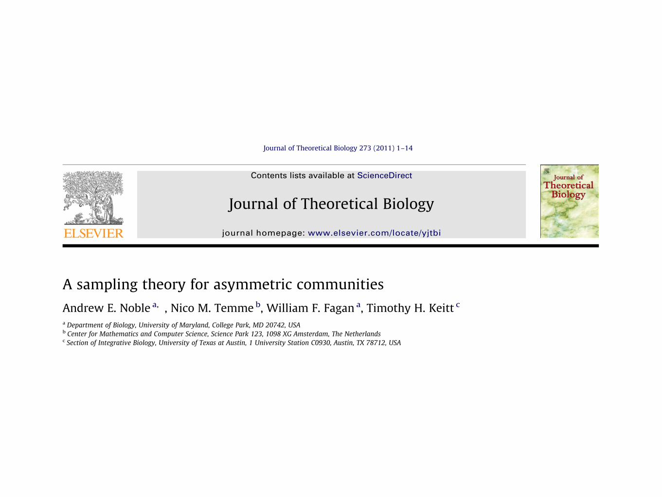
Current extinction rates are ~1000 times higher than the expected background.
At this rate, ~50% of present-day species will be extinct by 2100.
(UN Convention on Biological Diversity)
Motivation for Quantitative Modeling in Ecology
Goal: Predict observed patterns of species abundance and distribution based on a dynamical model prescribing interactions among the individuals of the coexisting species in a given area.
Central method: Specify rates of birth, death, migration, and speciation for a master equation where allowed abundances are the non-negative integers and the timing of demographic events are stochastic.
Quantitative Modeling of Community Ecology
The Appearance of Hypergeometric Functions
Univariate master equations with birth and death rates that are polynomial in the number of
individuals yield stationary distributions with a normalization given by a hypergeometric function.
Adrienne Kemp (1968)
J ! Community size > 10, 000 individuals
2F1that depends on


Journal of Computational and Applied Mathematics 153 (2003) 441–462www.elsevier.com/locate/cam
Large parameter cases of the Gauss hypergeometric functionNico M. Temme!
CWI, P.O. Box 94079, 1090 GB Amsterdam, Netherlands
Received 7 November 2001
Abstract
We consider the asymptotic behavior of the Gauss hypergeometric function when several of the parametersa; b; c are large. We indicate which cases are of interest for orthogonal polynomials (Jacobi, but also Meixner,Krawtchouk, etc.), which results are already available and which cases need more attention. We also considera few examples of 3F2 functions of unit argument, to explain which di!culties arise in these cases, whenstandard integrals or di"erential equations are not available.c! 2002 Elsevier Science B.V. All rights reserved.
MSC: 33C05; 33C45; 41A60; 30C15; 41A10
Keywords: Gauss hypergeometric function; Asymptotic expansion
1. Introduction
The Gauss hypergeometric function (see [1, chap. 15, 2, 30])
2F1
!
a; b
c; z
"
= 1 +abcz +
a(a+ 1)b(b+ 1)c(c + 1)2!
z2 + · · ·=!#
n=0
(a)n(b)n(c)nn!
zn; (1)
where Pochhammer’s symbol (a)n is de#ned by
(a)n =!(a+ n)!(a)
= ("1)nn!!
"a
n
"
; (2)
and the in#nite series in (1) is de#ned for |z|¡ 1 and c #= 0;"1;"2; : : : .
! Tel.: +20-592-4240; fax: +20-592-4199.E-mail address: [email protected] (N.M. Temme).
0377-0427/03/$ - see front matter c" 2002 Elsevier Science B.V. All rights reserved.PII: S0377-0427(02)00627-1

4/6/11 4:59 PMGmail - asymptotic expansions of 2F1
Page 1 of 1https://mail.google.com/mail/?ui=2&ik=d5ce93ba2a&view=pt&q=nico&qs=true&search=query&msg=120b528e30e23cf0
Andrew Noble <[email protected]>
asymptotic expansions of 2F1
Andrew Noble <[email protected]> Fri, Apr 17, 2009 at 1:39 PMTo: [email protected]
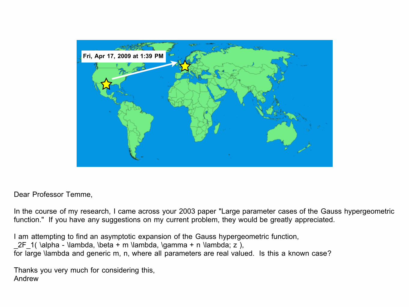
Dear Professor Temme,
In the course of my research, I came across your 2003 paper "Large parameter cases of the Gauss hypergeometricfunction." If you have any suggestions on my current problem, they would be greatly appreciated.
I am attempting to find an asymptotic expansion of the Gauss hypergeometric function, _2F_1( \alpha - \lambda, \beta + m \lambda, \gamma + n \lambda; z ), for large \lambda and generic m, n, where all parameters are real valued. Is this a known case?
Thanks you very much for considering this, Andrew
-----------------------------------------------------The University of Texas at AustinSection of Integrative Biology (BIO 223)1 University Station C0930Austin, TX 78712
4/6/11 4:59 PMGmail - asymptotic expansions of 2F1
Page 1 of 1https://mail.google.com/mail/?ui=2&ik=d5ce93ba2a&view=pt&q=nico&qs=true&search=query&msg=120b528e30e23cf0
Andrew Noble <[email protected]>
asymptotic expansions of 2F1
Andrew Noble <[email protected]> Fri, Apr 17, 2009 at 1:39 PMTo: [email protected]
Dear Professor Temme,
In the course of my research, I came across your 2003 paper "Large parameter cases of the Gauss hypergeometricfunction." If you have any suggestions on my current problem, they would be greatly appreciated.
I am attempting to find an asymptotic expansion of the Gauss hypergeometric function, _2F_1( \alpha - \lambda, \beta + m \lambda, \gamma + n \lambda; z ), for large \lambda and generic m, n, where all parameters are real valued. Is this a known case?
Thanks you very much for considering this, Andrew
-----------------------------------------------------The University of Texas at AustinSection of Integrative Biology (BIO 223)1 University Station C0930Austin, TX 78712

4/6/11 5:02 PMGmail - asymptotic expansions of 2F1
Page 1 of 1https://mail.google.com/mail/?ui=2&ik=d5ce93ba2a&view=pt&q=nico&qs=true&search=query&msg=120b582077d9dcb4
Andrew Noble <[email protected]>
asymptotic expansions of 2F1
Nico Temme <[email protected]> Fri, Apr 17, 2009 at 3:16 PMReply-To: [email protected]: Andrew Noble <[email protected]>Cc: [email protected]
Dear Andrew,
this is certainly not a known case; I will see what can be said about this. Are m and n positive? Perhaps integers?Also the value of the ratio m/n may be important. And is z < 1?
With best regards,
Nico.
[Quoted text hidden]
4/6/11 4:59 PMGmail - asymptotic expansions of 2F1
Page 1 of 1https://mail.google.com/mail/?ui=2&ik=d5ce93ba2a&view=pt&q=nico&qs=true&search=query&msg=120b528e30e23cf0
Andrew Noble <[email protected]>
asymptotic expansions of 2F1
Andrew Noble <[email protected]> Fri, Apr 17, 2009 at 1:39 PMTo: [email protected]
Dear Professor Temme,
In the course of my research, I came across your 2003 paper "Large parameter cases of the Gauss hypergeometricfunction." If you have any suggestions on my current problem, they would be greatly appreciated.
I am attempting to find an asymptotic expansion of the Gauss hypergeometric function, _2F_1( \alpha - \lambda, \beta + m \lambda, \gamma + n \lambda; z ), for large \lambda and generic m, n, where all parameters are real valued. Is this a known case?
Thanks you very much for considering this, Andrew
-----------------------------------------------------The University of Texas at AustinSection of Integrative Biology (BIO 223)1 University Station C0930Austin, TX 78712

Outline
Origins of the Project
Niche and Neutral Coexistence Mechanisms
Breaking the Symmetry of Neutral Theory
Asymptotic Expansions of Hypergeometric Functions
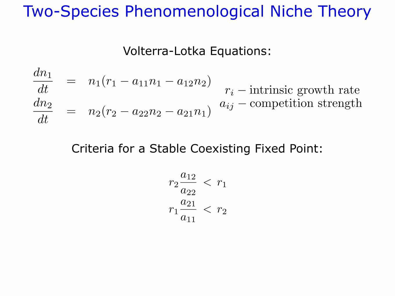
Two-Species Phenomenological Niche Theory
Criteria for a Stable Coexisting Fixed Point:
dn1
dt= n1(r1 ! a11n1 ! a12n2)
dn2
dt= n2(r2 ! a22n2 ! a21n1)
ri ! intrinsic growth rateaij ! competition strength
r2a12
a22< r1
r1a21
a11< r2
Volterra-Lotka Equations:
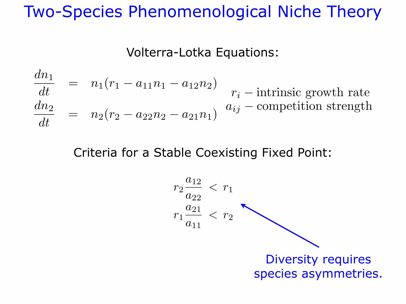
Two-Species Phenomenological Niche Theory
dn1
dt= n1(r1 ! a11n1 ! a12n2)
dn2
dt= n2(r2 ! a22n2 ! a21n1)
ri ! intrinsic growth rateaij ! competition strength
r2a12
a22< r1
r1a21
a11< r2
Volterra-Lotka Equations:
Diversity requires species asymmetries.
Criteria for a Stable Coexisting Fixed Point:

Consumer-Resource Niche Theory
Diversity requires species asymmetries.
The number of species at equilibrium is equal to the number of limiting resources.
Origins of Niche Theory222
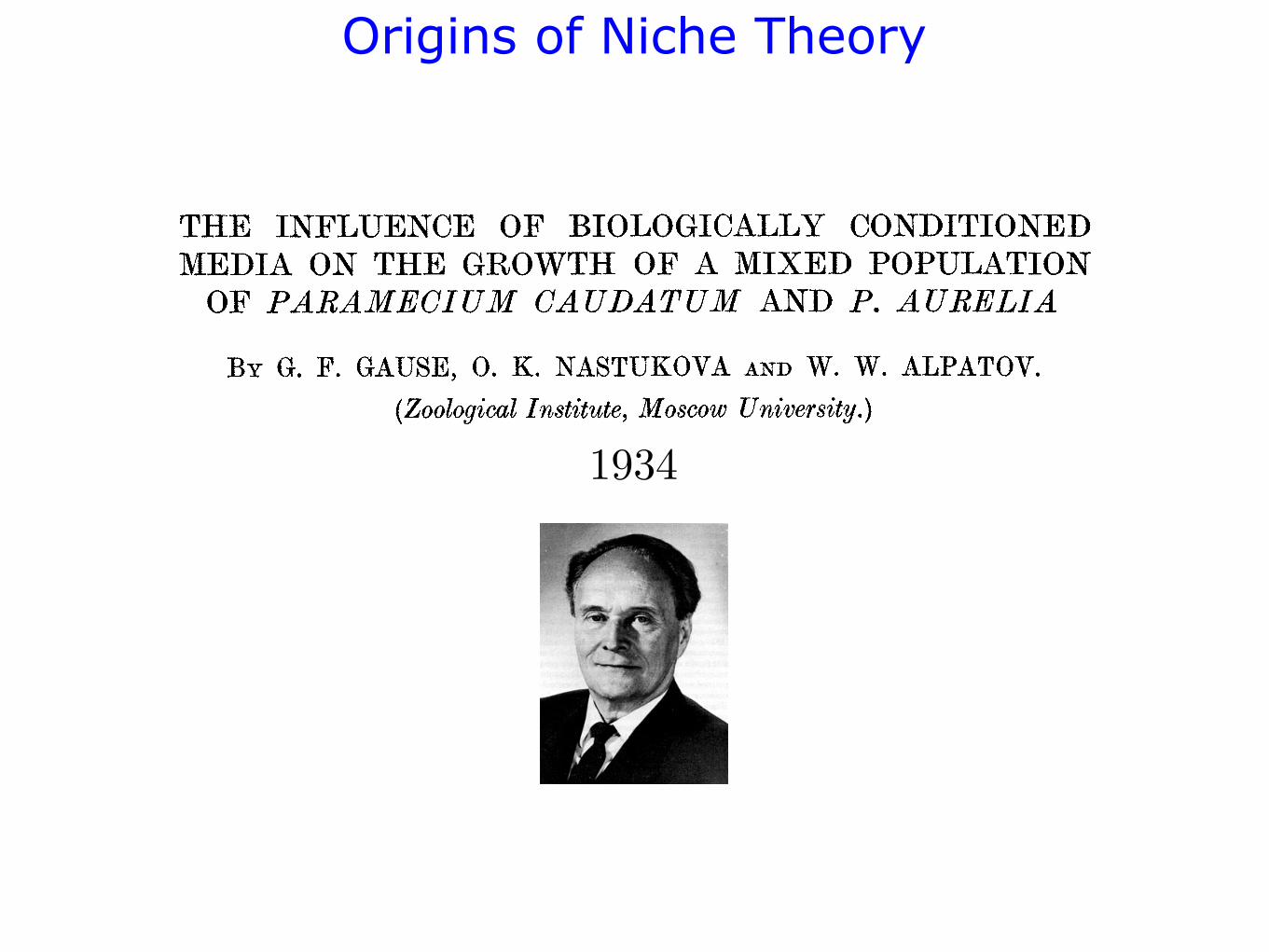
THE INFLUENCE OF BIOLOGICALLY CONDITIONED
MEDIA ON THE GROWTH OF A MIXED POPULATION
OF PARAMECIUM CAUDATUM AND P. AURELIA
BY G. F. GAUSE, 0. K. NASTUKOVA AND W. W. ALPATOV.
(Zoological Institute, Moscow University.)
(With six Figures in the Text.)
I. INTRODUCTION.
THE displacing of one species by another is apparently connected with the
advantages belonging to one of the competitors. In other terms one of them
is relatively better adapted to the habitat. The problem of relative adaptation
has been recently analysed theoretically by Fisher (4), but in spite of its
general interest it has hitherto been very insufficiently investigated on concrete
biological examples. The present paper is an account of the investigation on relative adaptation
in two species of Infusoria-Paramecium caudatum and P. aurelia-under
different conditions and at different stages of population growth. The case of
two similar species simplifies the analysis of certain general regularities of
competition in comparison with the study of similar races belonging to the
same species. Certain interesting observations showing the dependence of the relative
adaptation of two species of animals on environmental conditions have recently
appeared in ecological literature. For instance, Beauchamp and Ullyott (3)
have shown that when two species of Planaria in the English Lake District
occur in competition with one another, temperature is the factor which governs
the relative success and efficiency of the two species. Timofeeff-Ressovsky (9), dealing with the two species of fruit-fly Drosophila, has arrived at the same
conclusions. We have studied in this paper the action of biologically con-
ditioned media, containing waste products of the organisms that have lived in
them before. We had to deal with the influence of homotypic and heterotypic con-
ditioning (produced by organisms of the same and of a different species) on
the growth of a mixed population. As Woodruff (10) showed in his classical
paper, heterotypic conditioning in certain cases has much less influence on
the rate of reproduction of Infusoria than homotypic conditioning. In the
papers which have appeared since, the question of species specificity of the
conditioning has not attracted the attention it deserves-as Allee (1) has
1934
Origins of Niche Theory
G. F. GAUSE, 0. K. NASTUKOVA AND W. W. ALPATOV 225
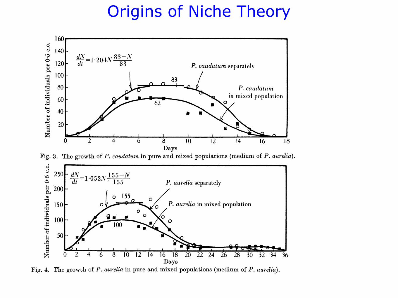
Figs. 1, 2, 3 and 4 show graphically the changes in the populations. One
can see that the first stage-growth of the populations-is generally completed
6 300 d 1-
00 d 21 2 p. aurelia separately
O 250I
Ca 200 ?
040> U P. aureliw in mixed population
0 2 4 6 8 10 12 14 16 18 20 22 24 26 28 30 32 34
Days Fig. 2. The growth of P. aurelia in pure and mixed populations (medium of P. caudatum).
160
1 40 dN8- -~~1-204NV
,< 120 | ddtN 1-20>1 N 8383N P. caudaturm separately
100 Ca
80 t:80t- P. cattdatuml io mixed populatioin
60-
40 40
20
0 2 4 6 8 10 12 14 16 18 Days
Fig. 3. The growth of P. caudatum in pure and mixed populations (medium of P. aurelia).
, 250 0~O5N 155 - P. aurelia separately 200
o 155
Ca ~ ~ ~ ~ ~ ~ ~ Dy
F 150 of P aurelia in mixed population 0
l1oo g 0 00
0~~~ 0
50
z 024 6 8 101214 16 182022 24 262830 3234 36 Days
Fig. 4. The growth of P. aurelia in pure and mixed populations (medium of P. aurelia).
on the seventh day. The maximal level attained remains invariable up to
about the tenth day, and decline of the population only begins later on.
Journ. of Animal Ecology ITI 15
Origins of Niche Theory
G. F. GAUSE, 0. K. NASTUKOVA AND W. W. ALPATOV 225
Figs. 1, 2, 3 and 4 show graphically the changes in the populations. One
can see that the first stage-growth of the populations-is generally completed
6 300 d 1-
00 d 21 2 p. aurelia separately
O 250I
Ca 200 ?
040> U P. aureliw in mixed population
0 2 4 6 8 10 12 14 16 18 20 22 24 26 28 30 32 34
Days Fig. 2. The growth of P. aurelia in pure and mixed populations (medium of P. caudatum).
160
1 40 dN8- -~~1-204NV
,< 120 | ddtN 1-20>1 N 8383N P. caudaturm separately
100 Ca
80 t:80t- P. cattdatuml io mixed populatioin
60-
40 40
20
0 2 4 6 8 10 12 14 16 18 Days
Fig. 3. The growth of P. caudatum in pure and mixed populations (medium of P. aurelia).
, 250 0~O5N 155 - P. aurelia separately 200
o 155
Ca ~ ~ ~ ~ ~ ~ ~ Dy
F 150 of P aurelia in mixed population 0
l1oo g 0 00
0~~~ 0
50
z 024 6 8 101214 16 182022 24 262830 3234 36 Days
Fig. 4. The growth of P. aurelia in pure and mixed populations (medium of P. aurelia).
on the seventh day. The maximal level attained remains invariable up to
about the tenth day, and decline of the population only begins later on.
Journ. of Animal Ecology ITI 15
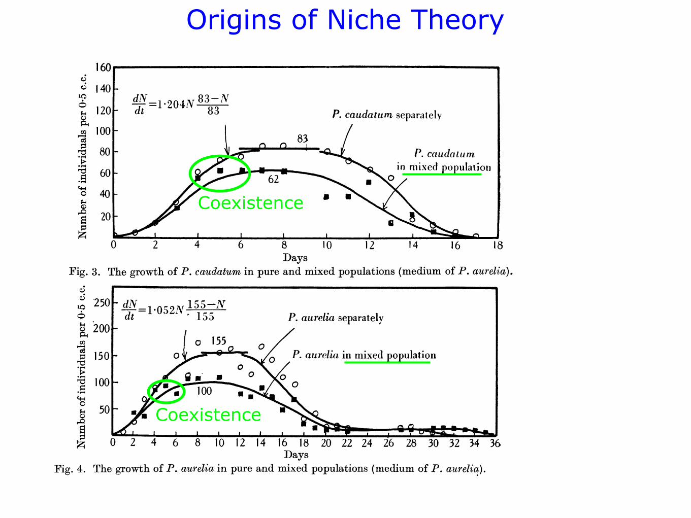
Coexistence
Coexistence
Origins of Niche Theory
G. F. GAUSE, 0. K. NASTUKOVA AND W. W. ALPATOV 225
Figs. 1, 2, 3 and 4 show graphically the changes in the populations. One
can see that the first stage-growth of the populations-is generally completed
6 300 d 1-
00 d 21 2 p. aurelia separately
O 250I
Ca 200 ?
040> U P. aureliw in mixed population
0 2 4 6 8 10 12 14 16 18 20 22 24 26 28 30 32 34
Days Fig. 2. The growth of P. aurelia in pure and mixed populations (medium of P. caudatum).
160
1 40 dN8- -~~1-204NV
,< 120 | ddtN 1-20>1 N 8383N P. caudaturm separately
100 Ca
80 t:80t- P. cattdatuml io mixed populatioin
60-
40 40
20
0 2 4 6 8 10 12 14 16 18 Days
Fig. 3. The growth of P. caudatum in pure and mixed populations (medium of P. aurelia).
, 250 0~O5N 155 - P. aurelia separately 200
o 155
Ca ~ ~ ~ ~ ~ ~ ~ Dy
F 150 of P aurelia in mixed population 0
l1oo g 0 00
0~~~ 0
50
z 024 6 8 101214 16 182022 24 262830 3234 36 Days
Fig. 4. The growth of P. aurelia in pure and mixed populations (medium of P. aurelia).
on the seventh day. The maximal level attained remains invariable up to
about the tenth day, and decline of the population only begins later on.
Journ. of Animal Ecology ITI 15
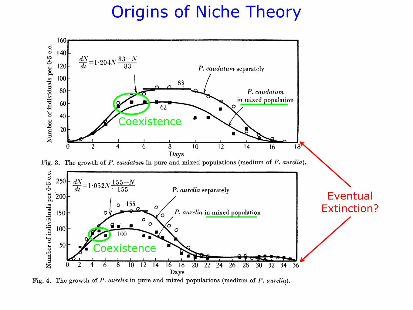
Coexistence
Coexistence
EventualExtinction?
2001
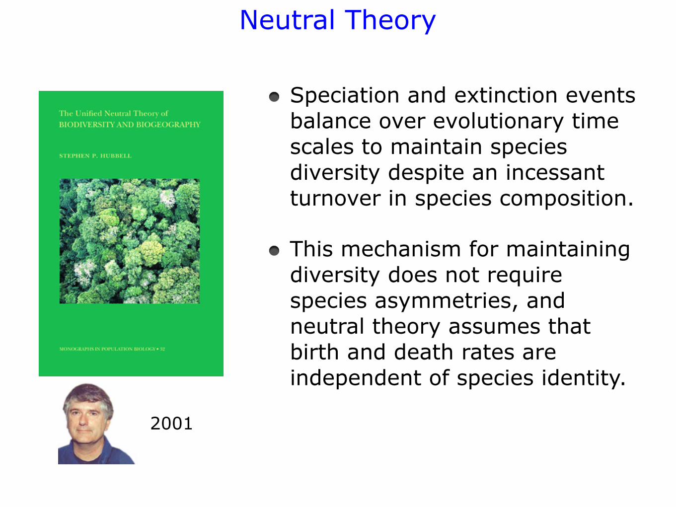
Neutral Theory
Speciation and extinction events balance over evolutionary time scales to maintain species diversity despite an incessant turnover in species composition.
This mechanism for maintaining diversity does not require species asymmetries, and neutral theory assumes that birth and death rates are independent of species identity.
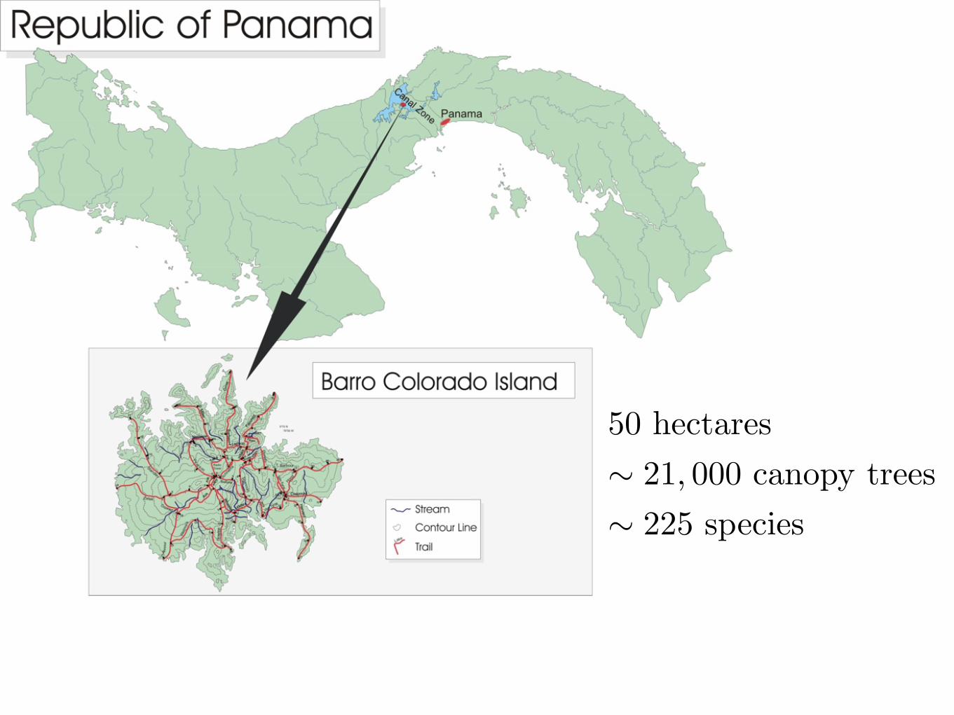
50 hectares! 21, 000 canopy trees! 225 species
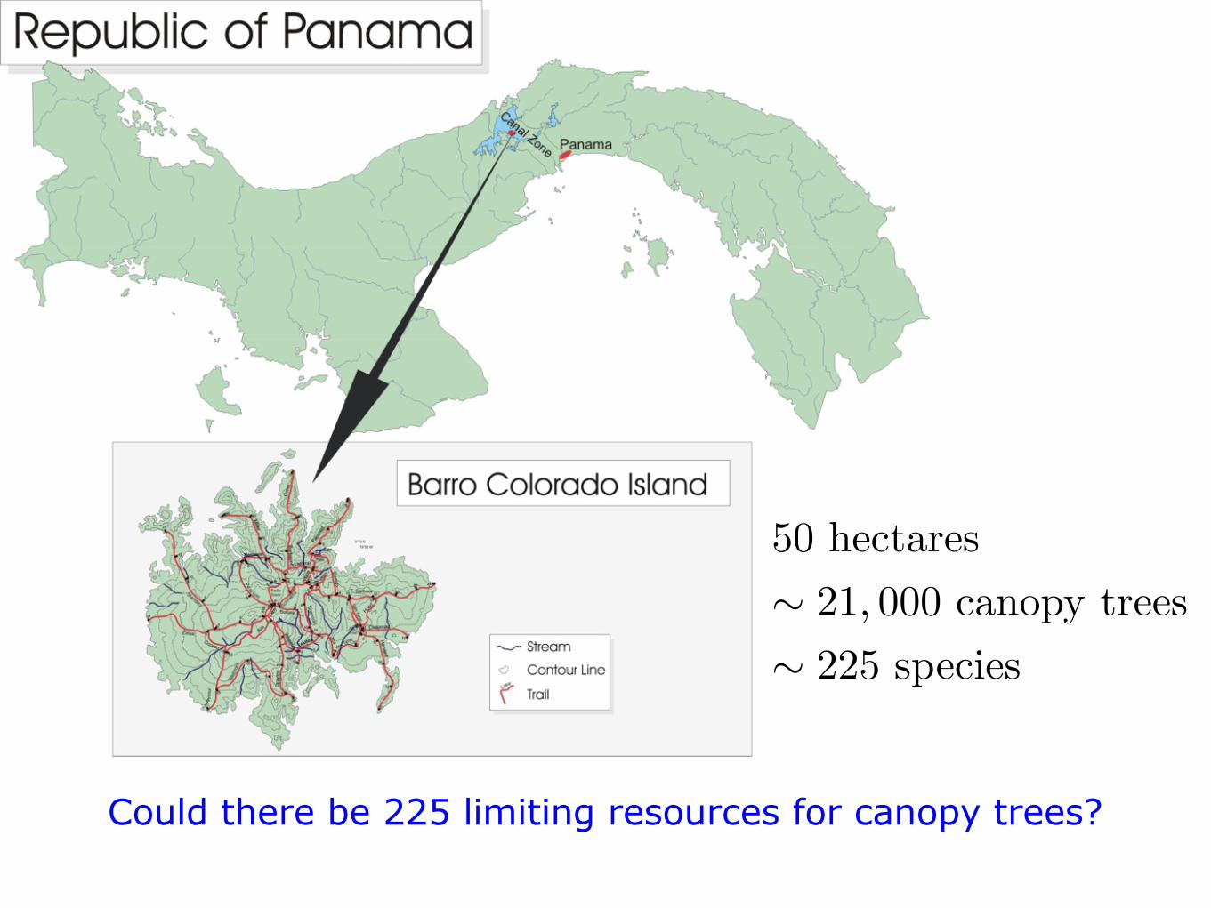
50 hectares! 21, 000 canopy trees! 225 species
Could there be 225 limiting resources for canopy trees?
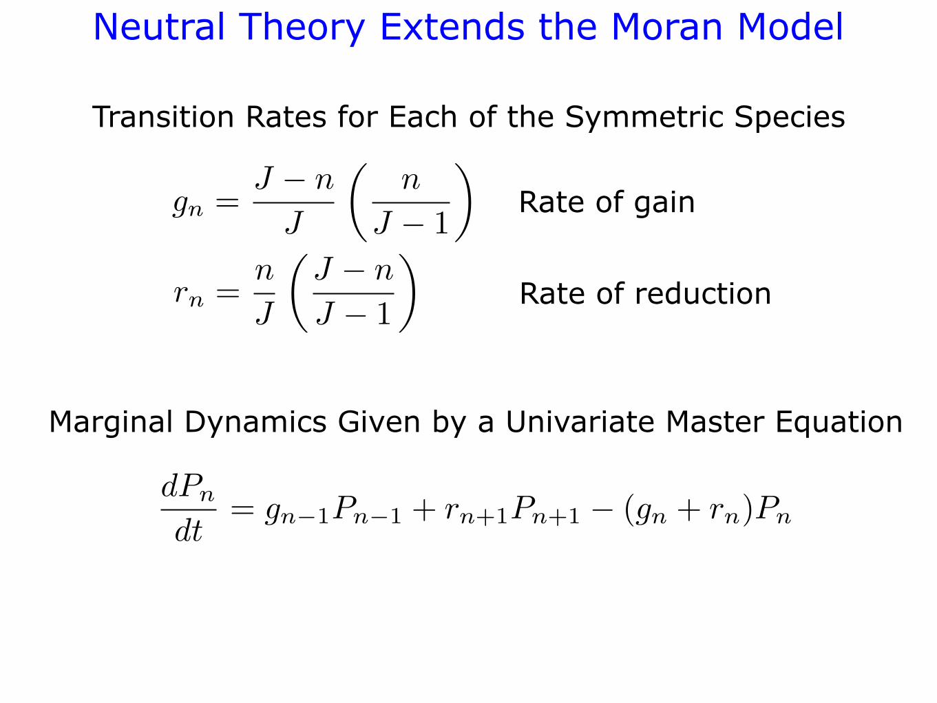
Neutral Theory Extends the Moran Model
Transition Rates for Each of the Symmetric Species
gn =J ! n
J
!n
J ! 1
"
rn =n
J
!J ! n
J ! 1
"
Marginal Dynamics Given by a Univariate Master Equation
dPn
dt= gn!1Pn!1 + rn+1Pn+1 ! (gn + rn)Pn
, probability of gain
, probability of loss
Rate of gain
Rate of reduction
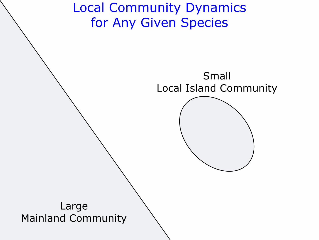
SmallLocal Island Community
LargeMainland Community
Local Community Dynamicsfor Any Given Species
Local Community Dynamicsfor Any Given Species
LargeMainland Community
Relative abundance
SmallLocal Island Community
x ! (0, 1)JL
A non-negative
integer number of individuals
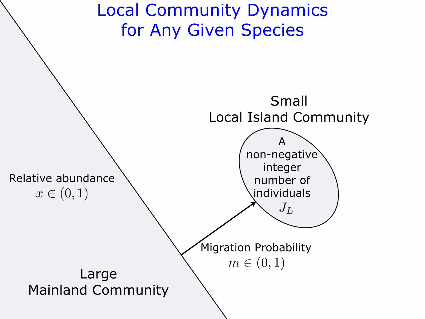
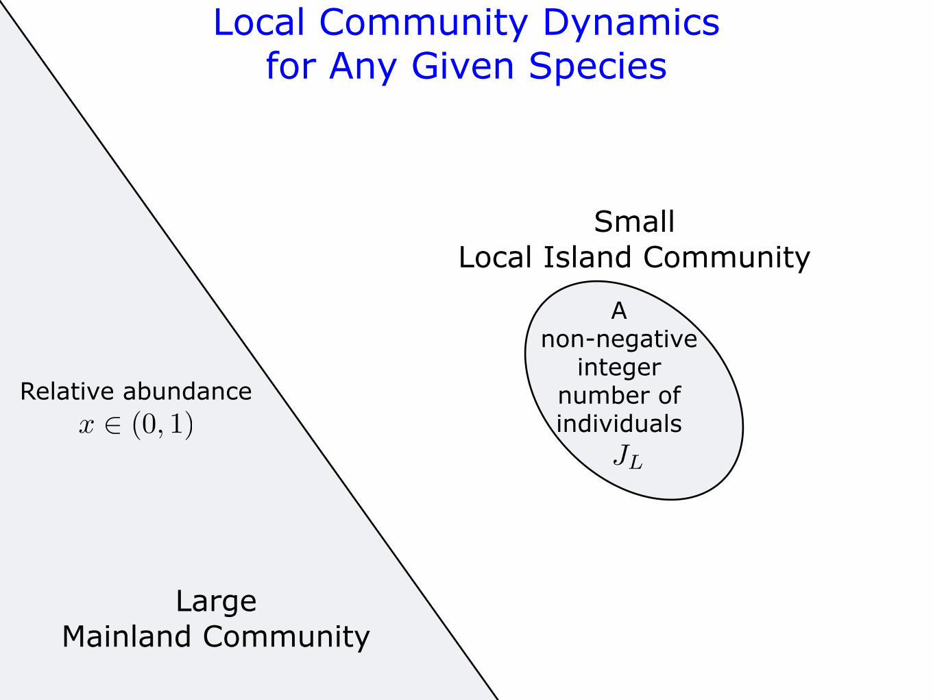
Local Community Dynamicsfor Any Given Species
LargeMainland Community
Relative abundance
SmallLocal Island Community
x ! (0, 1)JL
A non-negative
integer number of individuals
Migration Probabilitym ! (0, 1)
Neutral Theory
conservation of community size. One can show that the system isguaranteed to reach the stationary solution (2) in the infinite timelimit14.The frequency of species containing n individuals is given by:
fn !XS
k!1
Ik "3#
where S is the total number of species and the indicator I k is arandom variable which takes the value 1 with probability Pn,k and 0with probability (1 2 Pn,k). Thus the average number of speciescontaining n individuals is given by:
kfnl!XS
k!1
Pn;k "4#
The RSA relationship we seek to derive is the dependence of kfnlon n.Let a community consist of species with bn;k ; bn and dn;k ; dn
being independent of k (the species are assumed to be demographi-cally identical).From equation (4), it follows that kfnl is simply proportional to
Pn, leading to:
kfnl! SP0
Yn21
i!0
bidi$1
"5#
We consider a metacommunity in which the probability d that anindividual dies and the probability b that an individual gives birth toan offspring are independent of the population of the species towhich it belongs (density-independent case), that is, bn ! bn anddn ! dn"n. 0#: Speciation may be introduced by ascribing a non-zero probability of the appearance of an individual of a new species,that is, b0 ! v– 0: Substituting the expressions into equation (5),
one obtains the celebrated Fisher log series15:
kfMn l! SMP0
b0b1…bn21
d1d2…dn! v
xn
n"6#
where M refers to the metacommunity, x ! b/d and v! SMP0v=b isthe biodiversity parameter (also called Fisher’s a). We follow thenotation of Hubbell2 in this paper. Note that x represents the ratio ofeffective per capita birth rate to the death rate arising from a varietyof causes such as birth, death, immigration and emigration. Notethat in the absence of speciation, b0 ! v! v! 0; and, in equili-brium, there are no individuals in the metacommunity. When oneintroduces speciation, x has to be less than 1 to maintain a finitemetacommunity size JM !P
nnkfnl! vx=12 x:We turn now to the case of a local community of size Jundergoing
births and deaths accompanied by a steady immigration of indi-viduals from the surrounding metacommunity. When the localcommunity is semi-isolated from the metacommunity, one mayintroduce an immigration rate m, which is the probability ofimmigration from the metacommunity to the local community.For constant m (independent of species), immigrants belonging tothe more abundant species in the metacommunity will arrive in thelocal community more frequently than those of rarer species.
Our central result (see Box 1 for a derivation) is an analyticexpression for the RSA of the local community:
kfnl! vJ!
n!"J2 n#!G"g#
G"J$ g#
!g
0
G"n$ y#G"1$ y#
G"J2 n$ g2 y#G"g2 y#
exp"2yv=g#dy "7#
where G"z# !"10 t
z21e2tdt which is equal to (z 2 1)! for integer z
and g! m"J21#12m : As expected, kfnl is zero when n exceeds J. The
computer calculations in Hubbell’s book2 as well as those morerecently carried out by McGill3 were aimed at estimating kfnl bysimulating the processes of birth, death and immigration.
One can evaluate the integral in equation (7) numerically for agiven set of parameters: J, v andm. For large values of n, the integralcan be evaluated very accurately and efficiently using the method ofsteepest descent16. Any given RSA data set contains informationabout the local community size, J, and the total number of species inthe local community, SL !
PJk!1kfkl: Thus there is just one free
fitting parameter at one’s disposal.McGill asserted3 that the lognormal distribution is a more
parsimonious null hypothesis than the neutral theory, a suggestionwhich is not borne out by our reanalysis of the Barro ColoradoIsland (BCI) data. We focus only on the BCI data set because, aspointed out by McGill3, the North American Breeding Bird Surveydata are not as exhaustively sampled as the BCI data set, resulting infewer individuals and species in any given year in a given location.Furthermore, the McGill analysis seems to rely on adding the birdcounts over five years at the same sampling locations even thoughthese data sets are not independent.
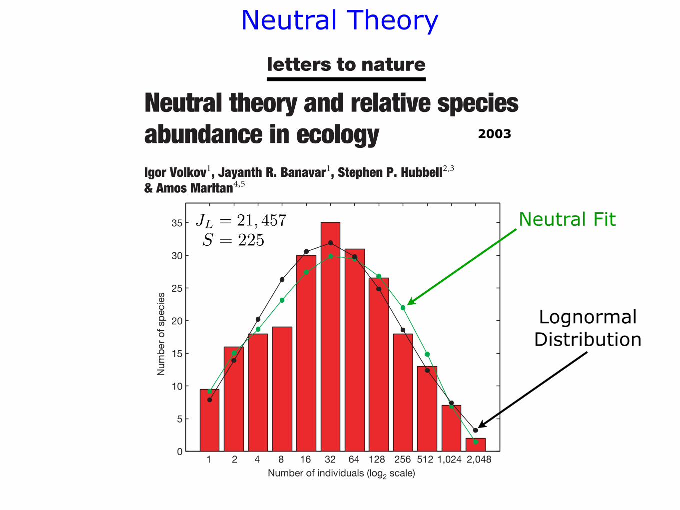
Figure 1 shows a Preston-like binning5 of the BCI data4 and the fitof our analytic expression with one free parameter (11 degrees offreedom) along with a lognormal having three free parameters (9degrees of freedom). Standard chi-square analysis17 yields values ofx2 ! 3.20 for the neutral theory and 3.89 for the lognormal. Theprobabilities of such good agreement arising by chance are 1.23%and 8.14% for the neutral theory and lognormal fits, respectively.Thus one obtains a better fit of the data with the analytical solutionto the neutral theory to BCI than with the lognormal, even thoughthere are two fewer free parameters. McGill’s analysis3 on the BCIdata set was based on computer simulations in which there weredifficulties in knowing when to stop the simulations, that is,when equilibrium had been reached. It is unclear whetherMcGill averaged over an ensemble of runs, which is essential toobtain repeatable and reliable results from simulations of stochastic
Figure 1 Data on tree species abundances in 50-hectare plot of tropical forest inBarro Colorado Island, Panama4. The total number of trees.10 cm DBH in the data set is
21,457 and the number of distinct species is 225. The red bars are observed numbers of
species binned into log2 abundance categories, following Preston’s method5. The first
histogram bar represents kf 1l/2, the second bar kf 1l/2 $ kf 2l/2, the third barkf 2l/2 $ kf 3l $ kf 4l/2 the fourth bar kf 4l/2 $ kf 5l $ kf 6l $ kf 7l $ kf 8l/2and so on. The black curve shows the best fit to a lognormal distribution
kfnl! Nn exp"2"log2n2 log2n0#2=2j2# (N ! 46.29, n 0 ! 20.82 and j ! 2.98),
while the green curve is the best fit to our analytic expression equation (7) (m ! 0.1 from
which one obtains v ! 47.226 compared to the Hubbell2 estimates of 0.1 and 50
respectively and McGill’s best fits3 of 0.079 and 48.5 respectively).
letters to nature
NATURE |VOL 424 | 28 AUGUST 2003 | www.nature.com/nature1036 © 2003 Nature Publishing Group
2003
..............................................................
Neutral theory and relative speciesabundance in ecologyIgor Volkov1, Jayanth R. Banavar1, Stephen P. Hubbell2,3
& Amos Maritan4,5
1Department of Physics, 104 Davey Laboratory, The Pennsylvania StateUniversity, University Park, Pennsylvania 16802, USA2Department of Plant Biology, The University of Georgia, Athens, Georgia 30602,USA3The Smithsonian Tropical Research Institute, Box 2072, Balboa, Panama4International School for Advanced Studies (SISSA), Via Beirut 2/4, 34014Trieste, Italy5INFM and The Abdus Salam International Center for Theoretical Physics,Trieste, Italy.............................................................................................................................................................................
The theory of island biogeography1 asserts that an island or alocal community approaches an equilibrium species richness as aresult of the interplay between the immigration of species fromthemuch larger metacommunity source area and local extinctionof species on the island (local community). Hubbell2 generalizedthis neutral theory to explore the expected steady-state distri-bution of relative species abundance (RSA) in the local commu-nity under restricted immigration. Here we present a theoreticalframework for the unified neutral theory of biodiversity2 and ananalytical solution for the distribution of the RSA both in themetacommunity (Fisher’s log series) and in the local community,where there are fewer rare species. Rare species are more extinc-tion-prone, and once they go locally extinct, they take longer tore-immigrate than do common species. Contrary to recentassertions3, we show that the analytical solution provides a betterfit, with fewer free parameters, to the RSA distribution of treespecies on Barro Colorado Island, Panama4, than the lognormaldistribution5,6.
The neutral theory in ecology2,7 seeks to capture the influence ofspeciation, extinction, dispersal and ecological drift on the RSAunder the assumption that all species are demographically alike on aper capita basis. This assumption, while only an approximation8–10,appears to provide a useful description of an ecological communityon some spatial and temporal scales2,7. More significantly, it allowsthe development of a tractable null theory for testing hypothesesabout community assembly rules. However, until now, there hasbeen no analytical derivation of the expected equilibrium distri-bution of RSA in the local community, and fits to the theory haverequired simulations2 with associated problems of convergencetimes, unspecified stopping rules, and precision3.
The dynamics of the population of a given species is governed bygeneralized birth and death events (including speciation, immigra-tion and emigration). Let bn,k and dn,k represent the probabilities ofbirth and death, respectively, in the kth species with n individualswith b21;k ! d0;k ! 0: Let pn,k(t) denote the probability that the kthspecies contains n individuals at time t. In the simplest scenario, thetime evolution of pn,k(t) is regulated by the master equation11–13
dpn;k"t#dt
! pn$1;k"t#dn$1;k $ pn21;k"t#bn21;k 2 pn;k"t#"bn;k
$ dn;k# "1#which leads to the steady-state or equilibrium solution, denoted byP:
Pn;k ! P0;k
Yn21
i!0
bi;kdi$1;k
"2#
for n . 0 and where P0,k can be deduced from the normaliza-tion condition
PnPn;k ! 1: Note that there is no requirement of
Box 1Derivation of the RSA of the local community
We study the dynamics within a local community following themathematical framework of McKane et al.27, who studied a mean-fieldstochastic model for species-rich communities. In our context, thedynamical rules2 governing the stochastic processes in thecommunity are:(1) With probability 1–m, pick two individuals at random from the
local community. If they belong to the same species, no action istaken.Otherwise, with equal probability, replace one of the individualswith the offspring of the other. In other words, the two individuals serveas candidates for death and parenthood.(2) With probability m, pick one individual at random from the local
community. Replace it by a new individual chosen with a probabilityproportional to the abundance of its species in the metacommunity.This corresponds to the death of the chosen individual in the localcommunity followed by the arrival of an immigrant from themetacommunity. Note that the sole mechanism for replenishingspecies in the local community is immigration from themetacommunity, which for the purposes of local community dynamicsis treated as a permanent source pool of species, as in the theory ofisland biogeography1.These rules are encapsulated in the following expressions for effective
birth and death rates for the kth species:
bn;k ! "12m#nJ
J2 n
J21$m
mkJM
12n
J
! ""8#
dn;k ! "12m#nJ
J2 n
J21$m 12
mkJM
# $n
J"9#
where mk is the abundance of the kth species in the metacommunityand JM is the total population of the metacommunity.The right hand side of equation (8) consists of two terms. The first
corresponds to rule (1) with a birth in the kth species accompanied by adeath elsewhere in the local community. The second term accountsfor an increase of the population of the kth species due to immigrationfrom the metacommunity. The immigration is, of course, proportionalto the relative abundance mk/JM of the kth species in themetacommunity. Equation (9) follows in a similar manner. Note thatbn,k and dn,k not only depend on the species label k but also are nolonger simply proportional to n.Substituting equation (8) and (9) into equation (2), one obtains the
expression27:
Pn;k !J!
n!"J2 n#!G"n$lk#G"lk#
G"ck 2 n#G"ck 2 J#
G"lk $ck 2 J#G"lk $ck#
; F"mk# "10#
where
lk !m
"12m# "J21# mkJM
"11#
and
ck ! J$ m
"12m# "J2 1# 12mkJM
# $"12#
Note that the k dependence in equation (10) enters only through mk.On substituting equation (10) into equation (4), one obtains:
kfnl!XSM
k!1
F"mk# ! SMkF"mk#l! SM
%dmr̂"m#F"m# "13#
Here r̂"m#dm is the probability distribution of the mean populations ofthe species in the metacommunity and has the form of the familiar Fisherlog series (in a singularity-free description15,28):
r̂"m#dm! 1
G"1#d1 exp"2m=d#m121dm "14#
where d ! x/(1 2 x). Substituting equation (14) into the integral inequation (13), taking the limits SM ! 1 and 1 ! 0 with v ! SM1approaching a finite value15,28 and on defining y ! m g
dv ; one can obtainour central result, equation (7).
letters to nature
NATURE |VOL 424 | 28 AUGUST 2003 | www.nature.com/nature 1035© 2003 Nature Publishing Group
JL = 21, 457S = 225
Neutral Fit
Lognormal Distribution

Outline
Origins of the Project
Niche and Neutral Coexistence Mechanisms
Breaking the Symmetry of Neutral Theory
Asymptotic Expansions of Hypergeometric Functions
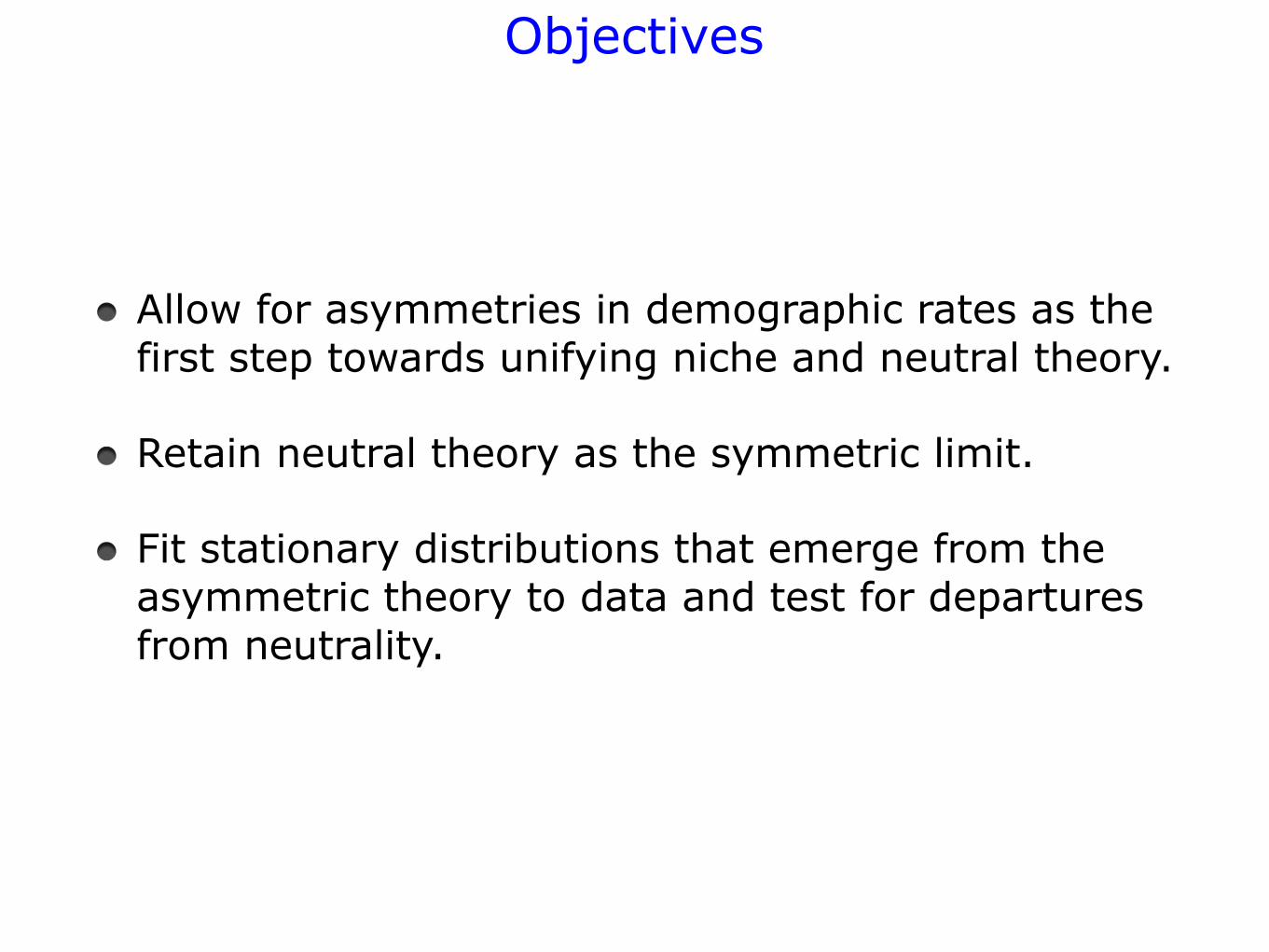
Objectives
Allow for asymmetries in demographic rates as the first step towards unifying niche and neutral theory.
Retain neutral theory as the symmetric limit.
Fit stationary distributions that emerge from the asymmetric theory to data and test for departures from neutrality.
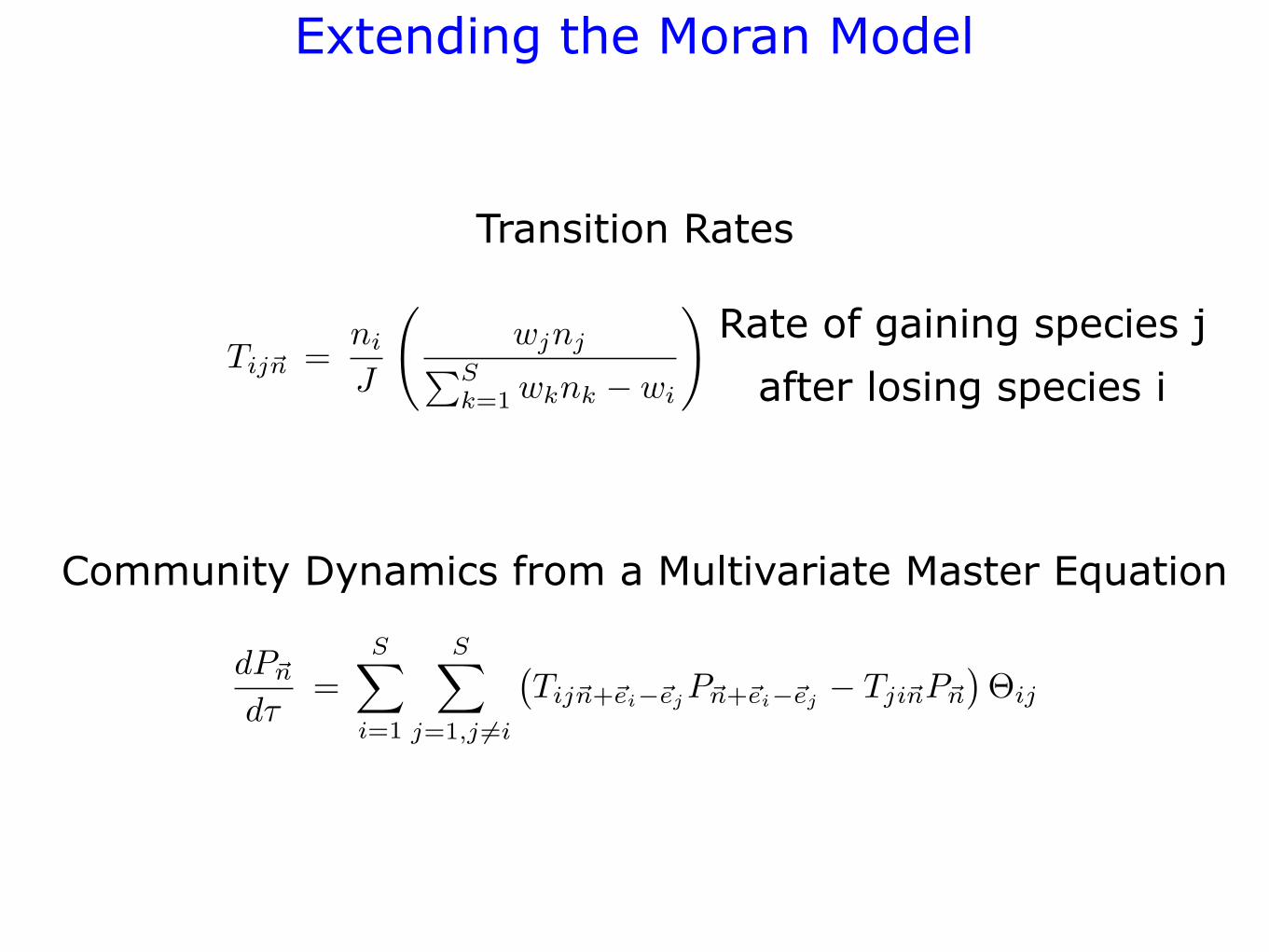
Extending the Moran Model
Transition Rates
Community Dynamics from a Multivariate Master Equation
, probability of lossRate of gaining species j
after losing species i
dP!n
d!=
S!
i=1
S!
j=1,j !=i
"Tij!n+!ei"!ej P!n+!ei"!ej ! Tji!nP!n
#!ij
Tij!n =ni
J
!wjnj"S
k=1 wknk ! wi
#
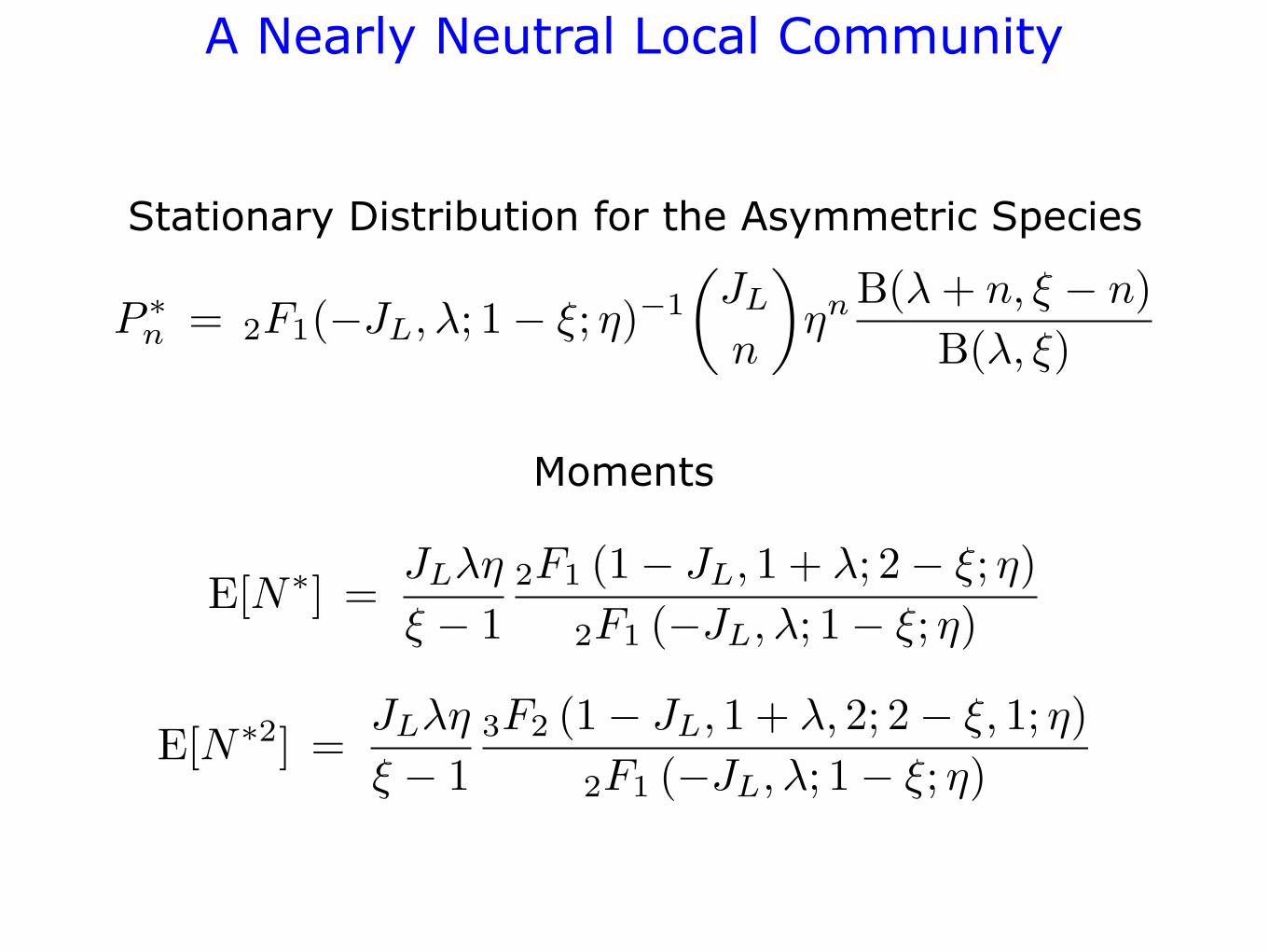
A Nearly Neutral Local Community
P !n = 2F1(!JL, !; 1! "; #)"1
!JL
n
"#n B(! + n, " ! n)
B(!, ")
Stationary Distribution for the Asymmetric Species
E[N!] =JL!"
# ! 12F1 (1! JL, 1 + !; 2! #; ")
2F1 (!JL, !; 1! #; ")
Moments
E[N!2] =JL!"
# ! 13F2 (1! JL, 1 + !, 2; 2! #, 1; ")
2F1 (!JL, !; 1! #; ")

Outline
Origins of the Project
Niche and Neutral Coexistence Mechanisms
Breaking the Symmetry of Neutral Theory
Asymptotic Expansions of Hypergeometric Functions
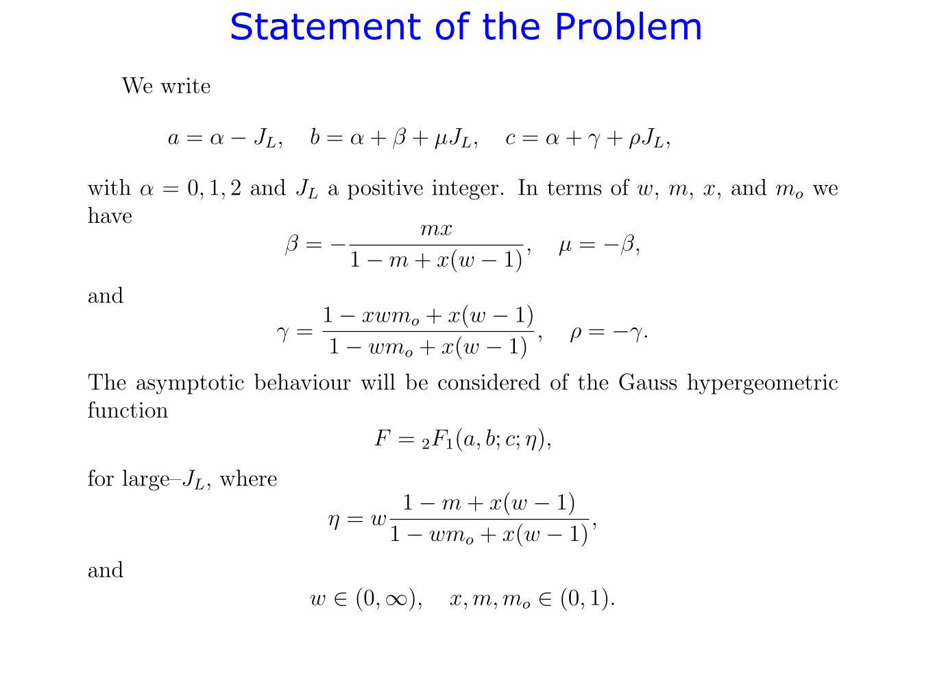
Statement of the ProblemAppendix C.2. Expanding 2F1(!! JL, ! + "; ! + 1! #; $)
Appendix C.2.1. NotationWe write
a = !! JL, b = ! + % + µJL, c = ! + & + 'JL, (C.2.1.1)
with ! = 0, 1, 2 and JL a positive integer. In terms of w, m, x, and mo wehave
% = ! mx
1!m + x(w ! 1), µ = !%, (C.2.1.2)
and
& =1! xwmo + x(w ! 1)
1! wmo + x(w ! 1), ' = !&. (C.2.1.3)
The asymptotic behaviour will be considered of the Gauss hypergeometricfunction
F = 2F1(a, b; c; $), (C.2.1.4)
for large–JL, where
$ = w1!m + x(w ! 1)
1! wmo + x(w ! 1), (C.2.1.5)
andw " (0,#), x,m, mo " (0, 1). (C.2.1.6)
Appendix C.2.2. The neutral case: w = 1, m = mo
In this case
$ = 1, µ =mx
1!m, ' = !1!mx
1!m. (C.2.2.1)
The exact relation
2F1(!n, b; c; 1) =(c! b)n
(c)n=
!(c)!(c! b + n)
!(c + n)!(c! b), n = 0, 1, 2, . . . , (C.2.2.2)
can be used, together with the asymptotic estimate of the ratio of gammafunctions
!(x + n)
!(y + n)= nx!y (1 +O(1/n)) , n$#. (C.2.2.3)
27
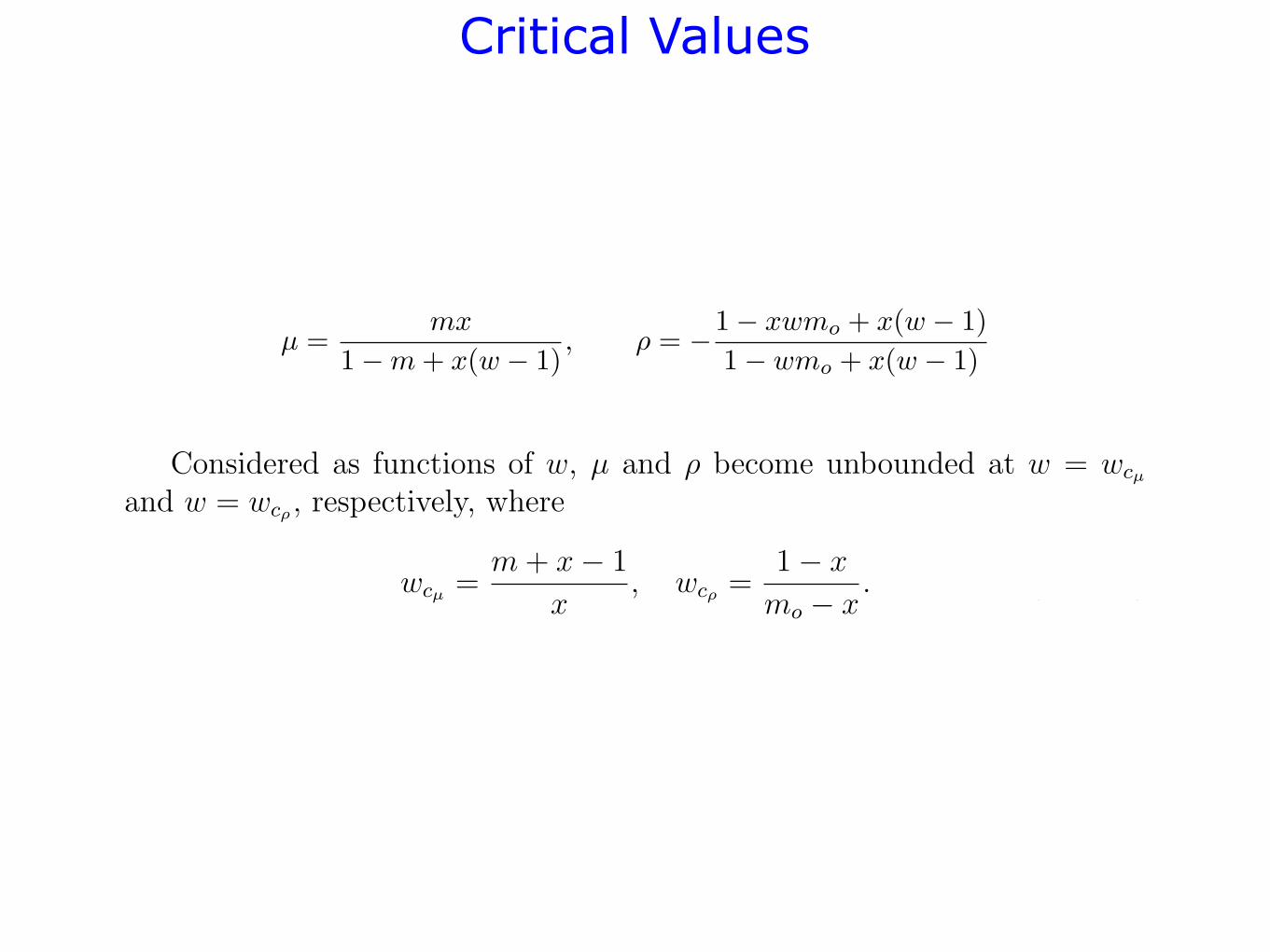
Critical Values
Appendix C.2.3. Critical valuesConsidered as functions of w, µ and ! become unbounded at w = wcµ
and w = wc! , respectively, where
wcµ =m + x! 1
x, wc! =
1! x
mo ! x. (C.2.3.1)
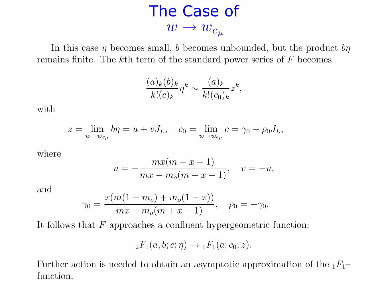
The case w " wcµ
In this case " becomes small, b becomes unbounded, but the product b"remains finite. The kth term of the standard power series of F becomes (seealso (C.2.2.3))
(a)k(b)k
k!(c)k"k # (a)k
k!(c0)kzk, (C.2.3.2)
with
z = limw!wcµ
b" = u + vJL, c0 = limw!wcµ
c = #0 + !0JL, (C.2.3.3)
where
u = ! mx(m + x! 1)
mx!mo(m + x! 1), v = !u, (C.2.3.4)
and
#0 =x(m(1!mo) + mo(1! x))
mx!mo(m + x! 1), !0 = !#0. (C.2.3.5)
It follows that F approaches a confluent hypergeometric function:
2F1(a, b; c; ")" 1F1(a; c0; z). (C.2.3.6)
Further action is needed to obtain an asymptotic approximation of the 1F1–function.
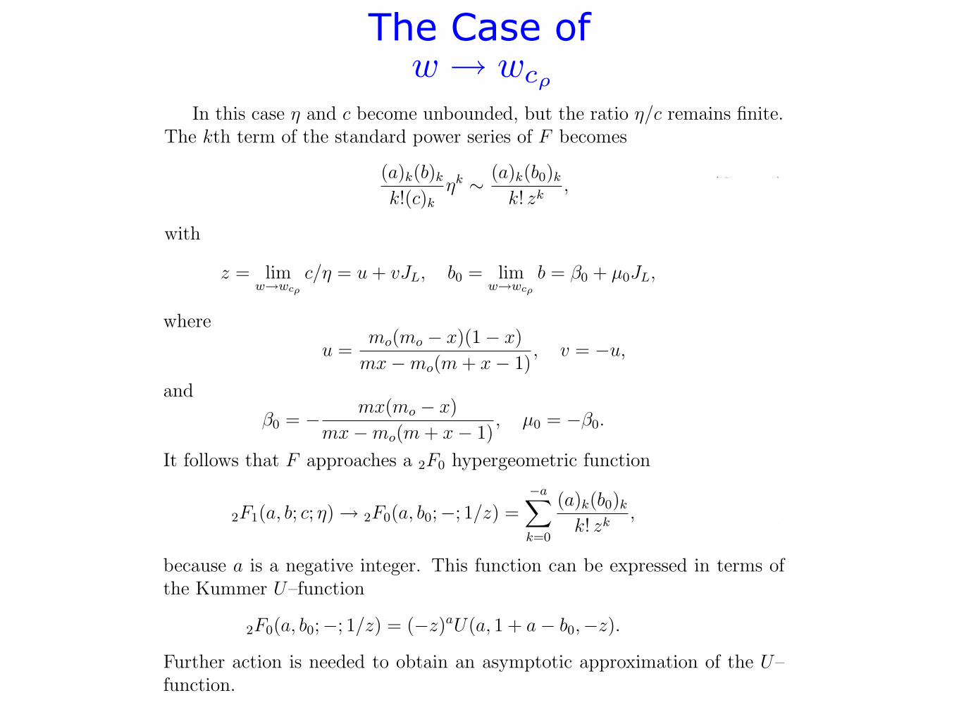
The case w " wc!
In this case " and c become unbounded, but the ratio "/c remains finite.The kth term of the standard power series of F becomes
(a)k(b)k
k!(c)k"k # (a)k(b0)k
k! zk, (C.2.3.7)
with
z = limw!wc!
c/" = u + vJL, b0 = limw!wc!
b = $0 + µ0JL, (C.2.3.8)
28
µ =mx
1!m + x(w ! 1), ! = !1! xwmo + x(w ! 1)
1! wmo + x(w ! 1)
The Case ofw ! wcµ
Appendix C.2.3. Critical valuesConsidered as functions of w, µ and ! become unbounded at w = wcµ
and w = wc! , respectively, where
wcµ =m + x! 1
x, wc! =
1! x
mo ! x. (C.2.3.1)
The case w " wcµ
In this case " becomes small, b becomes unbounded, but the product b"remains finite. The kth term of the standard power series of F becomes (seealso (C.2.2.3))
(a)k(b)k
k!(c)k"k # (a)k
k!(c0)kzk, (C.2.3.2)
with
z = limw!wcµ
b" = u + vJL, c0 = limw!wcµ
c = #0 + !0JL, (C.2.3.3)
where
u = ! mx(m + x! 1)
mx!mo(m + x! 1), v = !u, (C.2.3.4)
and
#0 =x(m(1!mo) + mo(1! x))
mx!mo(m + x! 1), !0 = !#0. (C.2.3.5)
It follows that F approaches a confluent hypergeometric function:
2F1(a, b; c; ")" 1F1(a; c0; z). (C.2.3.6)
Further action is needed to obtain an asymptotic approximation of the 1F1–function.
The case w " wc!
In this case " and c become unbounded, but the ratio "/c remains finite.The kth term of the standard power series of F becomes
(a)k(b)k
k!(c)k"k # (a)k(b0)k
k! zk, (C.2.3.7)
with
z = limw!wc!
c/" = u + vJL, b0 = limw!wc!
b = $0 + µ0JL, (C.2.3.8)
28
w ! wc!
The Case of
Appendix C.2.3. Critical valuesConsidered as functions of w, µ and ! become unbounded at w = wcµ
and w = wc! , respectively, where
wcµ =m + x! 1
x, wc! =
1! x
mo ! x. (C.2.3.1)
The case w " wcµ
In this case " becomes small, b becomes unbounded, but the product b"remains finite. The kth term of the standard power series of F becomes (seealso (C.2.2.3))
(a)k(b)k
k!(c)k"k # (a)k
k!(c0)kzk, (C.2.3.2)
with
z = limw!wcµ
b" = u + vJL, c0 = limw!wcµ
c = #0 + !0JL, (C.2.3.3)
where
u = ! mx(m + x! 1)
mx!mo(m + x! 1), v = !u, (C.2.3.4)
and
#0 =x(m(1!mo) + mo(1! x))
mx!mo(m + x! 1), !0 = !#0. (C.2.3.5)
It follows that F approaches a confluent hypergeometric function:
2F1(a, b; c; ")" 1F1(a; c0; z). (C.2.3.6)
Further action is needed to obtain an asymptotic approximation of the 1F1–function.
The case w " wc!
In this case " and c become unbounded, but the ratio "/c remains finite.The kth term of the standard power series of F becomes
(a)k(b)k
k!(c)k"k # (a)k(b0)k
k! zk, (C.2.3.7)
with
z = limw!wc!
c/" = u + vJL, b0 = limw!wc!
b = $0 + µ0JL, (C.2.3.8)
28where
u =mo(mo ! x)(1! x)
mx!mo(m + x! 1), v = !u, (C.2.3.9)
and
!0 = ! mx(mo ! x)
mx!mo(m + x! 1), µ0 = !!0. (C.2.3.10)
It follows that F approaches a 2F0 hypergeometric function
2F1(a, b; c; ")" 2F0(a, b0;!; 1/z) =!a!
k=0
(a)k(b0)k
k! zk, (C.2.3.11)
because a is a negative integer. This function can be expressed in terms ofthe Kummer U–function
2F0(a, b0;!; 1/z) = (!z)aU(a, 1 + a! b0,!z). (C.2.3.12)
Further action is needed to obtain an asymptotic approximation of the U–function.
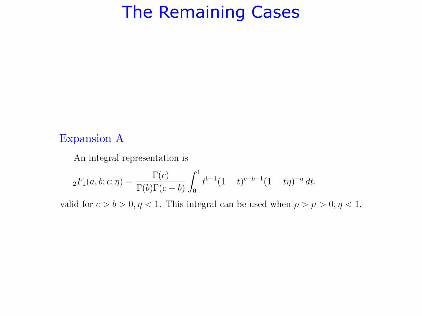
Appendix C.2.4. Expansion AAn integral representation is
2F1(a, b; c; ") =!(c)
!(b)!(c! b)
" 1
0
tb!1(1! t)c!b!1(1! t")!a dt, (C.2.4.1)
valid for c > b > 0, " < 1. This integral can be used when # > µ > 0, " < 1.As an example, consider
r = 3, m = 12 , mo = 1
2 , x = 13 . (C.2.4.2)
This gives
b = $ + 111(JL ! 1), c = $ + 5(JL ! 1), µ = 1
11 , # = 5, " = !11.(C.2.4.3)
In this case the integrand becomes small at t = 0 and t = 1, and there isa maximum of the integrand at t = t1, with t1 # (0, 1). This point gives themain contribution.
Write (C.2.4.1) as
2F1(a, b; c; ") =!(c)
!(b)!(c! b)
" 1
0
t!+"!1(1! t)#!"!1(1! t")!!e!JL$(t) dt,
(C.2.4.4)
29
The Remaining Cases
where
u =mo(mo ! x)(1! x)
mx!mo(m + x! 1), v = !u, (C.2.3.9)
and
!0 = ! mx(mo ! x)
mx!mo(m + x! 1), µ0 = !!0. (C.2.3.10)
It follows that F approaches a 2F0 hypergeometric function
2F1(a, b; c; ")" 2F0(a, b0;!; 1/z) =!a!
k=0
(a)k(b0)k
k! zk, (C.2.3.11)
because a is a negative integer. This function can be expressed in terms ofthe Kummer U–function
2F0(a, b0;!; 1/z) = (!z)aU(a, 1 + a! b0,!z). (C.2.3.12)
Further action is needed to obtain an asymptotic approximation of the U–function.
Appendix C.2.4. Expansion AAn integral representation is
2F1(a, b; c; ") =!(c)
!(b)!(c! b)
" 1
0
tb!1(1! t)c!b!1(1! t")!a dt, (C.2.4.1)
valid for c > b > 0, " < 1. This integral can be used when # > µ > 0, " < 1.As an example, consider
r = 3, m = 12 , mo = 1
2 , x = 13 . (C.2.4.2)
This gives
b = $ + 111(JL ! 1), c = $ + 5(JL ! 1), µ = 1
11 , # = 5, " = !11.(C.2.4.3)
In this case the integrand becomes small at t = 0 and t = 1, and there isa maximum of the integrand at t = t1, with t1 # (0, 1). This point gives themain contribution.
Write (C.2.4.1) as
2F1(a, b; c; ") =!(c)
!(b)!(c! b)
" 1
0
t!+"!1(1! t)#!"!1(1! t")!!e!JL$(t) dt,
(C.2.4.4)
29
Expansion A
The Remaining CasesExpansion B
Expansion C
The saddle points t0 and t1 are the zeros of !!(t). For the example (??) thisgives
t0 = !0.01169 · · · , t1 = 0.1178 · · · , (C.2.4.6)
and!(t1) = !0.02136 · · · , !!!(t1) = 35.83 · · · . (C.2.4.7)
An asymptotic approximation follows from the substitution
!(t)! !(t1) = 12!
!!(t1)s2, sign(t! t1) = sign(s), (C.2.4.8)
which gives
2F1(a, b; c; ") =!(c)
!(b)!(c! b)e"JL!(t1)
! #
"#f(s)e"
12JL!!!(t1)s2
ds, (C.2.4.9)
where
f(s) = t"+#"1(1! t)$"#"1(1! t")"" dt
ds. (C.2.4.10)
Because locally at t = t1 (or s = 0), t = t1 + s +O(s2), we have dt/ds = 1 ats = 0, and
f(0) = t"+#"11 (1! t1)
$"#"1(1! t1")"". (C.2.4.11)
This gives the first order approximation
2F1(a, b; c; ") " !(c)
!(b)!(c! b)e"JL!(t1)f(0)
! #
"#e"
12JL!!!(t1)s2
ds, (C.2.4.12)
that is
2F1(a, b; c; ") " !(c)
!(b)!(c! b)e"JL!(t1)f(0)
"2#
JL!!!(t1), JL #$.
(C.2.4.13)
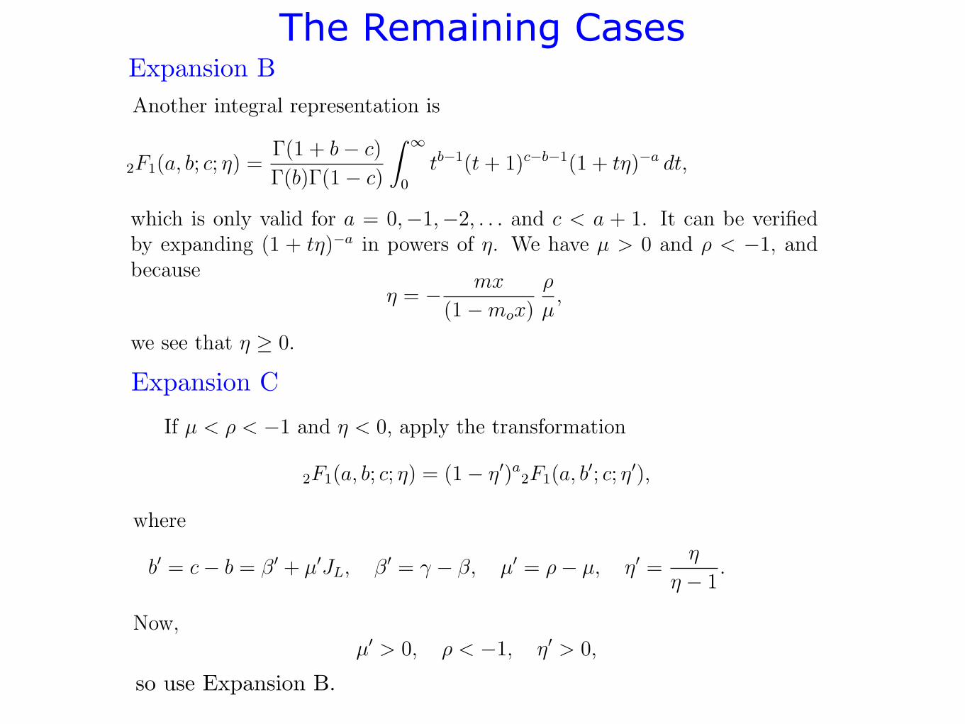
C.2.5. Expansion BAnother integral representation is
2F1(a, b; c; ") =!(1 + b! c)
!(b)!(1! c)
! #
0
tb"1(t + 1)c"b"1(1 + t")"a dt, (C.2.5.1)
29
which is only valid for a = 0,!1,!2, . . . and c < a + 1. It can be verifiedby expanding (1 + t!)!a in powers of !. We have µ > 0 and " < !1, andbecause
! = ! mx
(1!mox)
"
µ, (C.2.5.2)
we see that ! " 0.As an example, consider
r = 13 , m = 1
2 , mo = 12 , x = 1
3 . (C.2.5.3)
This gives
b = # + 3(JL ! 1), c = # + 1513(1! JL), µ = 3, " = !15
13 , ! = 113 .
(C.2.5.4)Write (??) as
2F1(a, b; c; !) =!(1 + b! c)
!(b)!(1! c)
! "
0
t!+"!1(t + 1)#!"!1(1 + t!)!!e!JL$(t) dt,
(C.2.5.5)where
$(t) = !µ ln(t)! ("! µ) ln(t + 1)! ln(1 + t!). (C.2.5.6)
The saddle points t0 and t1 are for the example (??)
t0 = !74.89 · · · , t1 = 3.385 · · · , (C.2.5.7)
and$(t1) = 2.251 · · · , $##(t1) = 0.04951 · · · . (C.2.5.8)
An asymptotic approximation follows from the substitution
$(t)! $(t1) = 12$
##(t1)s2, sign(t! t1) = sign(s), (C.2.5.9)
which gives
2F1(a, b; c; !) =!(1 + b! c)
!(b)!(1! c)e!JL$(t1)
! "
!"g(s)e!
12JL$!!(t1)s2
ds, (C.2.5.10)
where
g(s) = t!+"!1(1 + t)#!"!1(1 + t!)!! dt
ds. (C.2.5.11)
30
which gives
2F1(a, b; c; !) =!(1 + b! c)
!(b)!(1! c)e!JL!(t1)
! "
!"g(s)e!
12JL!!!(t1)s2
ds, (C.2.5.10)
where
g(s) = t"+#!1(1 + t)$!#!1(1 + t!)!" dt
ds. (C.2.5.11)
Because locally at t = t1 (or s = 0), t = t1 + s +O(s2), we have dt/ds = 1 ats = 0, and
g(0) = t"+#!11 (1 + t1)
$!#!1(1 + t1!)!". (C.2.5.12)
This gives the first order approximation
2F1(a, b; c; !) " !(1 + b! c)
!(b)!(1! c)e!JL!(t1)g(0)
! "
!"e!
12JL!!!(t1)s2
ds, (C.2.5.13)
that is
2F1(a, b; c; !) " !(1 + b! c)
!(b)!(1! c)e!JL!(t1)g(0)
"2"
JL###(t1), JL #$.
(C.2.5.14)
Appendix C.2.6. Expansion CIf µ < $ < !1 and ! < 0, apply the transformation
2F1(a, b; c; !) = (1! !#)a2F1(a, b#; c; !#), (C.2.6.1)
where
b# = c! b = %# + µ#JL, %# = & ! %, µ# = $! µ, !# =!
! ! 1. (C.2.6.2)
Now,µ# > 0, $ < !1, !# > 0, (C.2.6.3)
and it follows that Expansion B, §Appendix C.2.5, applies to the Gaussfunction on the right-hand side of (C.2.6.1).
32
so use Expansion B.
The Remaining Cases
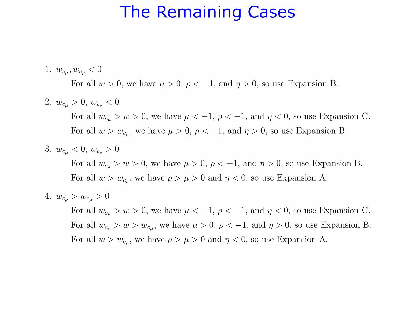
1. wcµ , wc! < 0
For all w > 0, we have µ > 0, ! < !1, and " > 0, so use Expansion B.
2. wcµ > 0, wc! < 0
For all wcµ > w > 0, we have µ < !1, ! < !1, and " < 0, so use Expansion C.
For all w > wcµ , we have µ > 0, ! < !1, and " > 0, so use Expansion B.
3. wcµ < 0, wc! > 0
For all wc! > w > 0, we have µ > 0, ! < !1, and " > 0, so use Expansion B.
For all w > wc! , we have ! > µ > 0 and " < 0, so use Expansion A.
4. wc! > wcµ > 0
For all wcµ > w > 0, we have µ < !1, ! < !1, and " < 0, so use Expansion C.
For all wc! > w > wcµ , we have µ > 0, ! < !1, and " > 0, so use Expansion B.
For all w > wc! , we have ! > µ > 0 and " < 0, so use Expansion A.
C.3 Expanding 2F1(1! JM , 1; 2! #M ; "M)
C.3.1 Notation
We writea = 1! JM , b = 1, c = $ + %JM , (C.3.1.1)
with
$ = 1 +1
1! w&o, % = ! 1
1! w&o. (C.3.1.2)
The asymptotic behaviour will be considered of the Gauss hypergeometric function
F = 2F1(a, b; c; "M) (C.3.1.3)
for large–JM , where
"M =w(1! &)
1! w&o, (C.3.1.4)
andw " (0,#), &, &o " (0, 1). (C.3.1.5)
C.3.2 The neutral case: w = 1, & = &o
In this case "M = 1 and (C.2.2.2) can be used to get an exact result in terms of gamma functions.
C.3.3 The critical case wc"o= 1/&o
In this case we have (see also §C.2.3)
2F1(a, b; c; "M)$ 2F0(a, b;!; 1/z) = (!z)aU(a, 1 + a! b,!z), (C.3.3.1)
where
z = !(JM ! 1)&o
1! &. (C.3.3.2)
19
Additional Work for the Mainland Model
Expanding 2F1(1! JM , 1; 2! !M ; "M ) and 3F2(1! JM , 1, 1; 2, 2! !M ; "M ).
Summary
For a problem in ecological modeling, we have derived a great number of expansions of hypergeometric functions by identifying critical parameter values and enumerating special cases.
In a few cases, the asymptotics can only be described by using their limits in the form of confluent hypergeometric functions.
Future research is needed to develop uniform transitions among the great number of special cases.


![ASYMPTOTIC EXPANSIONS FOR RATIOS OF PRODUCTS OF …downloads.hindawi.com/journals/ijmms/2003/953101.pdf · ASYMPTOTIC EXPANSIONS FOR RATIOS OF PRODUCTS... 1171 [3] R. B. Dingle, Asymptotic](https://img.pdfslide.net/doc/110x75/5f0746b27e708231d41c2ef3/asymptotic-expansions-for-ratios-of-products-of-asymptotic-expansions-for-ratios.jpg)