Embed Size (px)
Citation preview
Novel Mathematical Aspects of
Phylogenetic Estimation
A thesis submitted by
Mareike Fischer
in partial fulfillment of the requirements for the degree
Doctor of Philosophy
at the University of Canterbury
Examining Committee
Prof. Mike Steel: Internal Examiner
Prof. David Penny: External (NZ) Examiner
Prof. Arndt von Haeseler: External (overseas) Examiner

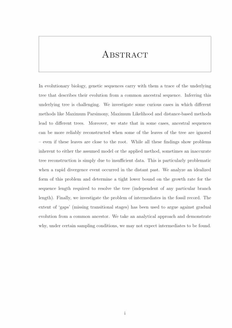
Abstract
In evolutionary biology, genetic sequences carry with them a trace of the underlying
tree that describes their evolution from a common ancestral sequence. Inferring this
underlying tree is challenging. We investigate some curious cases in which different
methods like Maximum Parsimony, Maximum Likelihood and distance-based methods
lead to different trees. Moreover, we state that in some cases, ancestral sequences
can be more reliably reconstructed when some of the leaves of the tree are ignored
– even if these leaves are close to the root. While all these findings show problems
inherent to either the assumed model or the applied method, sometimes an inaccurate
tree reconstruction is simply due to insufficient data. This is particularly problematic
when a rapid divergence event occurred in the distant past. We analyze an idealized
form of this problem and determine a tight lower bound on the growth rate for the
sequence length required to resolve the tree (independent of any particular branch
length). Finally, we investigate the problem of intermediates in the fossil record. The
extent of ‘gaps’ (missing transitional stages) has been used to argue against gradual
evolution from a common ancestor. We take an analytical approach and demonstrate
why, under certain sampling conditions, we may not expect intermediates to be found.
i

ii

Acknowledgements
I take this opportunity to thank my supervisor Mike Steel for his support over the last
three years. By explaining relevant concepts and pointing out various open problems
he made it easy for me to access the area of phylogenetics, which was new to me when
I first came to New Zealand. Moreover, he always took the time to discuss the progress
of my work, such that any problems at which I got stuck could be sorted out quickly.
Most importantly, he encouraged me right from the beginning to present my results at
various conferences, where I also got to meet many researchers from a variety of different
areas. These experiences have definitely contributed to the value the last three years
had both for my personal as well as my professional life.
Additionally, I want to thank my other two co-authors Hans-Jurgen Bandelt and
Bhalchandra Thatte. With both I had many fruitful discussions, which gave rise to
various mathematical ideas. Moreover, Bhalchandra often took the time to look at
my other projects and to give me helpful comments on them. Also, I thank Wolfgang
Fischl for the great collaboration concerning the relevance of ‘misleading sequences’ in
practice.
I wish to thank my co-supervisors Barbara Holland and Charles Semple, as well as
my external PhD examiners Arndt von Haeseler and David Penny. I will remember all
my visits to Palmerston North, during which I had many opportunities to present my
own work as well as to be introduced to open questions on which Barbara and David
were working, as great times – in spite of the weather in Palmy, which tried very hard
to convince me otherwise. The same applies to my visit to Arndt’s working group in
Vienna, where despite the unbearable heat many fruitful mathematical discussions took
place. I also owe many thanks to Marta Casanellas, who invited me to her working
iii

iv Novel Mathematical Aspects of Phylogenetic Estimation
group in Barcelona and introduced me to Elizabeth Allman and John Rhodes. All three
of them, Marta, Elizabeth and John, showed a lot of interest in my work and made
many useful suggestions. I also thank the Alfred Renyi Institute of Mathematics in
Budapest for enabling me to stay there and collaborate with Bhalchandra, but also for
giving me the opportunity to discuss my work with Peter Erdos and Laszlo Skekeley.
This was very helpful.
During the past three years, I attended about 15 conferences and meetings and I
additionally visited four different working groups. At all these occasions, I had useful
mathematical discussions with many different people – so, naturally, it is impossible to
thank all of them. But I do wish to explicitly thank Elliott Sober, who brought the
problem of intermediate fossils to my attention, as well as Matt Philips, who told me
about the importance of clades in biological research, and Oliver Will, who gave me
some additional information on the fossil record.
All of the above mentioned people made my time in New Zealand worthwhile and
unforgettable. But there are several others who made it even more invaluable: Beata
Faller, Ramona Schmid and Simone Linz – I thank you for all the coffees, walks, trips
and thoughts we shared. I remember that I once told you that our friendship developed
in time-lapse speed, and I still think that this is the reason why I felt at home in New
Zealand so quickly. Thanks, Madels, for everything!
I also wish to thank all other postgraduate students and postdocs I met in New
Zealand and who brightened up many of my days. To name just a few of them: Alethea,
Tanja, Klaas, Erick, Scott, Daniel, Hannes, Michael, Iris, Maarten and Meghan. More-
over, thanks to all my fellow Stats tutors, most importantly Irene David, Hilary Seddon,
Anna MacDonald, Miriam Hodge and, of course, the best colleague and officemate ever:
Kyoko Fukuda. Thanks for tolerating all my boxes for the last couple of months! I also
absolutely have to thank Rachael, Peter, Nicole, Joshua, Michael, Shannon and Liene
for the very best night during the last three years – as well as their support on the

v
worst morning ever, which directly followed that night.
Despite all these great people, my time in New Zealand would not have been the
same without the backup and support of my family and friends back home in Europe.
First of all, thanks to everyone who visited me here: Eva and Andreas, I knew you
would like the cave! Christian and Taiga, I will never forget our evening at that very
peculiar bar my sister suggested. And Julia, I am glad you could come here after all
– it has been great to see you growing up, and it was even better to be able to show
you one of the most beautiful countries in the world. Thanks also to you, Britta, Kata
and Oli – I know you wanted to visit me, but it did not work out in the end. I am
thankful for all your support over the last decade. Particular thanks also to Thomas
and Hannah – I lack the words to describe how glad I am to have friends like you.
Most importantly, I want to thank my family for their support and, particularly
my parents, for coping with the long journey just to visit me here – I know that for
you these long flights are even worse than for me. My sister Janina has always been
invaluable – she is inspiring and funny, and we are the best team ever (even though
some of the things we take up often just cause incredulous head shaking of our parents
and others). Thanks for being the only chemistry student in the world voluntarily
proofreading a maths PhD thesis, and even more thanks for coming to New Zealand
twice and joining every weird activity this country has to offer – the photo taken during
our paraflight is still my favorite.
I also wish to thank the New Zealand Mathematical Society for awarding me the
Aitken Prize. And, most importantly, I am much obliged to the Allan Wilson Centre
for Molecular Ecology and Evolution and the Marsden Fund for financing my research.
Without their support, all this would not have been possible.
Thanks to all of you and to this country, Aotearoa, for the best 3 years of my life.
Mareike Fischer

vi
Contents
Abstract i
Acknowledgement iii
1 Introduction 1
2 Preliminaries 5
2.1 Basic Definitions and Notations . . . . . . . . . . . . . . . . . . . . . . 5
2.2 The Nr-model . . . . . . . . . . . . . . . . . . . . . . . . . . . . . . . . 6
2.3 Phylogenetic Methods . . . . . . . . . . . . . . . . . . . . . . . . . . . 7
2.3.1 Maximum Parsimony . . . . . . . . . . . . . . . . . . . . . . . . 7
2.3.2 Maximum Likelihood . . . . . . . . . . . . . . . . . . . . . . . . 9
2.3.3 Distance-based Methods . . . . . . . . . . . . . . . . . . . . . . 9
3 Maximum Parsimony on Subsets of Taxa 13
3.1 The MP Reconstruction Accuracy of the Root State . . . . . . . . . . . 14
3.2 An Example of a Misleading Taxon . . . . . . . . . . . . . . . . . . . . 16
3.3 A Single Taxon under a Molecular Clock . . . . . . . . . . . . . . . . . 19
3.4 Interpretation . . . . . . . . . . . . . . . . . . . . . . . . . . . . . . . . 22
4 Misleading Sequences 25
4.1 Construction of Misleading Sequences from Ternary Characters . . . . 26
4.1.1 Illustration . . . . . . . . . . . . . . . . . . . . . . . . . . . . . 32
4.1.2 Sequence Length Analysis . . . . . . . . . . . . . . . . . . . . . 33
4.2 A Characterization of Misleading Sequences for Four Taxa . . . . . . . 38
vii
viii Novel Mathematical Aspects of Phylogenetic Estimation
4.3 Relevance of Misleading Sequences in Practice . . . . . . . . . . . . . . 45
4.4 Interpretation . . . . . . . . . . . . . . . . . . . . . . . . . . . . . . . . 48
5 Equivalence of Maximum Parsimony and Maximum Likelihood 51
5.1 Elementary Proof of the Tuffley-Steel Result . . . . . . . . . . . . . . . 52
5.2 Bounded Substitution Probabilities . . . . . . . . . . . . . . . . . . . . 58
5.3 Molecular Clock . . . . . . . . . . . . . . . . . . . . . . . . . . . . . . . 67
5.3.1 Analysis of Binary Characters under a Molecular Clock . . . . . 70
5.4 Interpretation . . . . . . . . . . . . . . . . . . . . . . . . . . . . . . . . 74
6 Resolving Deep Divergences 77
6.1 Preliminaries . . . . . . . . . . . . . . . . . . . . . . . . . . . . . . . . 79
6.2 Lower Bounds . . . . . . . . . . . . . . . . . . . . . . . . . . . . . . . . 81
6.3 An Upper bound: The Performance of Maximum Parsimony . . . . . . 84
6.4 The Performance of MP under the Random Cluster Model . . . . . . . 92
6.5 Lower Bounds for More General Models . . . . . . . . . . . . . . . . . 93
6.6 Interpretation . . . . . . . . . . . . . . . . . . . . . . . . . . . . . . . . 97
7 Expected Anomalies in the Fossil Record 99
7.1 Preliminaries . . . . . . . . . . . . . . . . . . . . . . . . . . . . . . . . 101
7.2 An Approach based on Evolutionary History . . . . . . . . . . . . . . . 103
7.3 Cladistic Approach . . . . . . . . . . . . . . . . . . . . . . . . . . . . . 110
7.4 Interpretation . . . . . . . . . . . . . . . . . . . . . . . . . . . . . . . . 116
8 Conclusion and Outlook 119
Appendix 123
List of Symbols 127

CONTENTS ix
List of Figures 129
List of Tables 131
Index 133
Publications Resulting from this Thesis 137
Bibliography 139

x Novel Mathematical Aspects of Phylogenetic Estimation
Chapter 1
Introduction
All sciences, arts and religions are branches of the same tree.
Albert Einstein
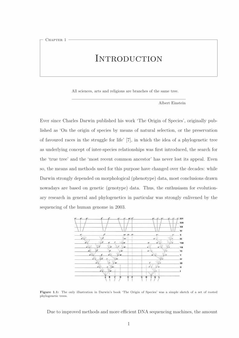
Ever since Charles Darwin published his work ‘The Origin of Species’, originally pub-
lished as ‘On the origin of species by means of natural selection, or the preservation
of favoured races in the struggle for life’ [7], in which the idea of a phylogenetic tree
as underlying concept of inter-species relationships was first introduced, the search for
the ‘true tree’ and the ‘most recent common ancestor’ has never lost its appeal. Even
so, the means and methods used for this purpose have changed over the decades: while
Darwin strongly depended on morphological (phenotype) data, most conclusions drawn
nowadays are based on genetic (genotype) data. Thus, the enthusiasm for evolution-
ary research in general and phylogenetics in particular was strongly enlivened by the
sequencing of the human genome in 2003.
Figure 1.1: The only illustration in Darwin’s book ‘The Origin of Species’ was a simple sketch of a set of rootedphylogenetic trees.
Due to improved methods and more efficient DNA sequencing machines, the amount
1
2 Novel Mathematical Aspects of Phylogenetic Estimation
of available DNA sequence data is ever-growing. Unsurprisingly, this makes phyloge-
netic models and methods, which help interpret the data, more and more essential. In
this thesis, we present the most important of these models and methods along with some
innovative results. We first present some general preliminaries in Chapter 2, in which
the methods and models used in this thesis are introduced along with some required
terminology. Then, we analyze these methods more in-depth. First, we show in Chap-
ter 3 that there are cases in which the Fitch algorithm for Maximum Parsimony (MP),
which is one of the most frequently used phylogenetic methods, gives more accurate
estimates of the ancestral root state when some taxa, i.e., leaves of the underlying tree,
are ignored – even if these taxa are close to the root. In Chapters 4, 5 and 6, we analyze
the performance and accuracy of different tree reconstruction methods: first, in Chapter
4, we show that for all numbers of taxa ternary sequences can be constructed for which
the perfect MP tree does not coincide with the distance-wise perfect tree. We show
how to construct such ‘misleading’ sequences and we present a full characterization of
them for the 4-taxa case. In Chapter 5, we show that MP and another tree inference
method, Maximum Likelihood (ML), may choose conflicting trees for certain biologi-
cally relevant modifications of the so-called ‘no common mechanism’ Nr-model, even
though they are known to be equivalent without these modifications. In particular, we
show that the equivalence fails when a molecular clock is assumed or when nucleotide
substitution probabilities are bounded by an upper bound less than that assumed by
the Nr-model (under ‘no common mechanism’). We will also explain to what extent
the latter inequivalence is related to the misleading sequences as introduced in Chapter
4. Then, in Chapter 6, we analyze the general accuracy of tree reconstruction methods
for a worst-case scenario: when speciation events occurred in rapid succession (leading
to short branch lengths) in the distant past (leading to the large branch lengths for
the incident edges), this makes the underlying tree particularly difficult to reconstruct.
We analyze a somewhat idealized 4-taxa case and provide tight lower bounds (up to a
constant factor) on the sequence length needed to reconstruct the true tree with high
probability.
Introduction 3
Finally, in Chapter 7 we introduce two simple stochastic models (one based on the
amount of evolutionary history and another one based on clades of the underlying tree)
for the estimation of the degree of relatedness of fossils from different times. We show
that there are cases in which fossils from an intermediate time cannot be expected to
be morphological intermediates – and thus will cause alleged ‘gaps’ in the fossil record.
This is a novel approach to explain anomalies in the fossil record, as traditionally only
reasons like the rare conditions needed for fossilization and the discontinuous fossil
discovery (as opposed to continuous evolutionary processes) are specified.
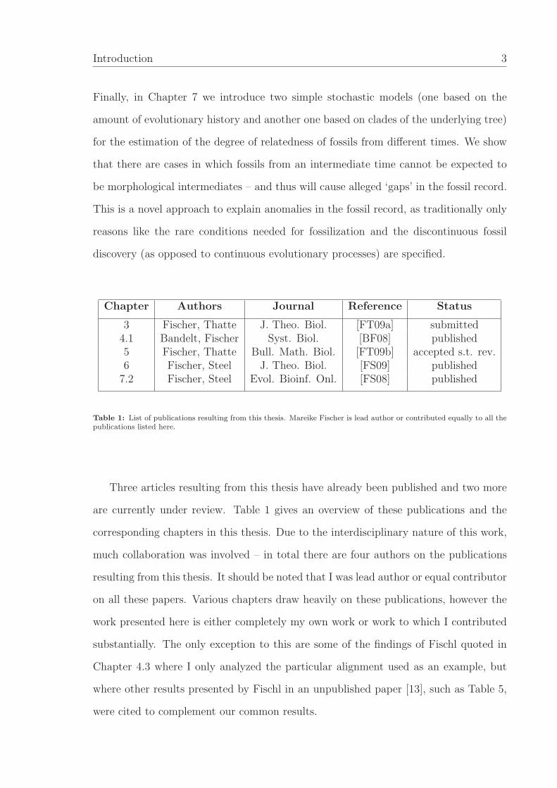
Chapter Authors Journal Reference Status
3 Fischer, Thatte J. Theo. Biol. [FT09a] submitted4.1 Bandelt, Fischer Syst. Biol. [BF08] published5 Fischer, Thatte Bull. Math. Biol. [FT09b] accepted s.t. rev.6 Fischer, Steel J. Theo. Biol. [FS09] published
7.2 Fischer, Steel Evol. Bioinf. Onl. [FS08] published
Table 1: List of publications resulting from this thesis. Mareike Fischer is lead author or contributed equally to all thepublications listed here.
Three articles resulting from this thesis have already been published and two more
are currently under review. Table 1 gives an overview of these publications and the
corresponding chapters in this thesis. Due to the interdisciplinary nature of this work,
much collaboration was involved – in total there are four authors on the publications
resulting from this thesis. It should be noted that I was lead author or equal contributor
on all these papers. Various chapters draw heavily on these publications, however the
work presented here is either completely my own work or work to which I contributed
substantially. The only exception to this are some of the findings of Fischl quoted in
Chapter 4.3 where I only analyzed the particular alignment used as an example, but
where other results presented by Fischl in an unpublished paper [13], such as Table 5,
were cited to complement our common results.

4 Novel Mathematical Aspects of Phylogenetic Estimation
Chapter 2
Preliminaries
2.1 Basic Definitions and Notations
We start with some basic definitions and general notations which will be used through-
out this thesis. Notations or definitions which are used only in one chapter will be
introduced where needed.
An unrooted phylogenetic X-tree is a tree T = (V (T ), E(T )) with vertices V (T )
and edges E(T ) on a leaf set X = {1, . . . , n} ⊆ V (T ) with no vertices of degree 2. If T
is binary, all internal nodes have degree 3. Note that a binary phylogenetic tree on X
has n leaves (end nodes) that are labeled by the n taxa in X and n − 2 interior nodes
that are unlabeled. The definition of rooted phylogenetic X-trees is analogous except
that there one node of degree 2, namely the root, is allowed. A character f is a function
f : X → C for some set C := {c1, c2, c3, . . . , cr} of r character states (r ∈ N) and is often
denoted by f = α1 . . . αn, where αi ∈ C for all i = 1, . . . , n, and where f(i) = αi. A
character is said to be informative (with respect to parsimony) if at least two distinct
character states occur more than once in X, otherwise it is called uninformative or
non-informative. Moreover, we say that each character induces a partition of X: if,
for instance, f = αβγ . . . γ, f induces the partition 1|2|3 . . . n, or, more formally, the
partition of X into the sets {1}, {2} and {3, . . . , n}. If f is binary, the induced partition
is called an X-split or split for short. Partitions and splits of X are said to be trivial
exactly when they are induced by non-informative characters on X. Throughout this
thesis, we will use the following notation (see [38]): Let Σ(X) be the set of all X-splits
σ = A|B = B|A of a set X of n taxa, i.e. Σ(X) = {σ = A|B = B|A : A ∪ B =
X,A ∩ B = ∅}. Furthermore, let Σ∗(X) be the set of non-trivial X-splits only (i.e.
5
6 Novel Mathematical Aspects of Phylogenetic Estimation
the set of X-splits for which |A|, |B| > 1). Analogously, let Σ(T ) denote the X-splits
induced by the edges of T (where T is an binary phylogenetic X-tree), and Σ∗(T ) the
non-trivial ones.
An extension of a character f to V (T ) is a map g : V (T ) → C such that the
restriction of g to X ⊆ V (T ) is f . For such an extension g of f , we denote by lT (g) the
number of edges e = (u, v) in T on which a substitution occurs, i.e., where g(u) 6= g(v).
Often, we analyze a sequence of characters rather than a single character. If a
sequence S consists of characters f1, . . . , fk for some integer k ≥ 1, we denote this by
S = f1 . . . fk. If two sequences S = f1 . . . fk and S = f1 . . . fl are concatenated, the
concatenation is denoted by sequence S = SS = f1 . . . fkf1 . . . fl.
2.2 The Nr-model
We now introduce the nucleotide substitution model on which most of our results are
based. Unless stated otherwise, our results will correspond to the so-called Nr-model,
also known as r-state symmetric model, Neyman r-state model or Cavender-Farris-
Neyman model. For r = 4, the Nr-model is also known as Jukes-Cantor model [20].
Let T be a phylogenetic X-tree, and let c1, . . . , cr be r distinct character states.
If T is not rooted, we may arbitrarily choose one of the leaves to be the root (note
that because of the so-called reversibility of the Nr-model, the actual root position
does not matter, see [11]). Then, the Nr-model assumes a uniform distribution of
states at the root, and assumes equal rates of substitutions between any two distinct
character states [31]. For any edge e ∈ E(T ), let pe denote the probability that a
substitution of a character state ci by another character state cj occurs on edge e for
ci 6= cj. Furthermore, let qe denote the probability that no substitution occurs on edge
e. Then, in the Nr-model we have 0 ≤ pe ≤ 1r
for all e ∈ E(T ) and (r − 1)pe + qe = 1.
Furthermore, the Nr-model assumes that substitutions occur independently on different
Preliminaries 7
edges.
Although it is the simplest non-trivial Markov process on a tree, the Nr-model
allows for an exact analysis of many scenarios. Moreover, stochastic results for this
model typically extend to more general finite-state models where an exact analysis is
usually more complex [28].
Note that for the interpretation of character sequences S = f1 . . . fm as opposed
to single characters, we often make the additional model assumption of ‘no common
mechanism’. This means that substitution probabilities on edges of the underlying tree
T may differ for each character in the sequence without any correlation between the
sites. That is, we suppose that for each character fi in the sequence and for each edge e
of the tree, there is a parameter pe,i that gives the substitution probability for fi on edge
e, and that the parameters pe,i are all independent. For all i = 1, . . . ,m, we will denote
by pi the vector of substitution probabilities pe,i assigned to the edges e of T . So the
difference between the Nr-model and the Nr-model with the additional assumption of
no common mechanism is that for a sequence S = f1 . . . fm of characters, both assume
that all characters evolved independently, but when there is a common mechanism, the
distributions of the characters additionally have to be identical (i.e., pe,i = pe for all
i and some fixed value pe). So whenever characters evolve ‘i.i.d.’, there is a common
mechanism.
We will introduce other models, such as the Random Cluster Model, in Chapters
6.4 and 6.5.
2.3 Phylogenetic Methods
2.3.1 Maximum Parsimony
Maximum Parsimony, or MP for short, is one of the most frequently used tree inference
8 Novel Mathematical Aspects of Phylogenetic Estimation
methods, and it is not based on a specific nucleotide substitution model. It selects the
tree that requires the smallest number of substitutions to extend the sequences at the
tips of the tree to (ancestral) sequences at all the interior vertices of the tree. Its
simplest form is the so-called Fitch parsimony [14], which will be considered in this
thesis unless stated otherwise. Given a character f and a tree T , MP assigns sets of
character states to all internal nodes such that they provide possible choices to achieve
the minimum number of changes to realize f . Along the way, the so-called parsimony
score or MP-score lT (f), which denotes the minimum number of changes required to
realize f on T , is calculated. It is obtained by minimizing lT (g) over all possible
extensions g of f . The parsimony score of a sequence of characters S := f1f2 . . . fm is
given by lT (S) =m∑
i=1
lT (fi). In order to use MP for tree inference, all possible trees
have to be analyzed. A (not necessarily unique) tree with minimal parsimony score
is called Maximum Parsimony tree, or MP-tree for short. Note that a parsimoniously
non-informative character has the same MP-score on all trees, whereas informative
characters have different scores on at least two trees. If an r-state character f has
parsimony score r − 1 on a tree T , it is said to be convex or homoplasy-free on T . A
sequence of characters is called convex or homoplasy-free on T when all its characters
have this property. If a sequence is convex on a tree T , T is called its perfect phylogeny.
Note that when MP is used for tree inference in Chapters 4, 5 and 6, unless stated
otherwise, the term most parsimonious extension g of a character f on a tree T refers
to any extension g for which lT (g) is minimal. The minimal MP-score can be calculated
with the Fitch algorithm given in [14]. However, in Chapter 3, where the reconstruction
accuracy of MP concerning the ancestral root state is examined, we consider only those
interior node labels and thus extensions which are suggested by the Fitch algorithm. It
is important to state this as it is known that while the Fitch algorithm calculates the
parsimony score and gives some most parsimonious extensions, it does not necessarily
find all most parsimonious extensions (see [12], pp. 12–13 for details). For further
background on MP, the reader can consult, for example, [12] or [38].
Preliminaries 9
2.3.2 Maximum Likelihood
Now we define Maximum Likelihood trees, or for short ML-trees. As opposed to MP,
ML is based on nucleotide substitution models and thus may give different results for
different models. In this thesis, we assume the Nr-model when inferring ML-trees. Note
that in the Nr-model, the parameter space is compact, which is why we can here define
ML-trees using only maxima rather than suprema.
For any phylogenetic X-tree T , any character f on the leaf set X and any vector
p of substitution probabilities assigned to all edges of T , we denote by P (f |T , p) the
likelihood of observing the character f on T for the given parameter values p. The max-
imum likelihood of a character f on T , denoted by max P (f |T ), is then the maximum
of P (f |T , p) over the space of all p, i.e., maxp P (f |T , p).
When the likelihood of a character sequence S is calculated, we assume ‘no common
mechanism’, i.e., if pe,i gives the substitution probability for fi on edge e, we assume
that the parameters pe,i are all independent. For a sequence S := f1 . . . fm the likelihood
is the product of the likelihoods of the individual characters, i.e., P (S|T , p1, . . . , pm) =m∏
i=1
P (fi|T , pi). Then, under no common mechanism, the maximum likelihood of S can
be calculated as the product of the maximum likelihoods of the individual characters,
i.e., max(p1,...,pm) P (S|T , p1, . . . , pm) =m∏
i=1
maxpiP (fi|T , pi). Finally, the (not necessarily
unique) Maximum Likelihood tree, or ML-tree for short, of S is a tree for which this
value is maximal, i.e., argmaxT max(p1,...,pm) P (S|T , p1, . . . , pm).
An algorithm for the explicit calculation of ML-trees is given by Felsenstein [11].
2.3.3 Distance-based Methods
Apart from various variations of MP and ML, the third group of most frequently used
tree inference methods are distance-based methods such as, for instance, Neighbor-
Joining [3]. In this thesis, we only consider the simplest kind of distances, namely
10 Novel Mathematical Aspects of Phylogenetic Estimation
the so-called non-normalized Hamming distance, which is also known as mismatch dis-
tance. In practice, these distances are normally used in a ‘corrected’ form to account
for so-called hidden changes in sequence evolution (for instance, if both a sequence and
one of its ancestral sequences have an A at a particular site, this does not mean that no
change has occurred during the sequence evolution – e.g., the A could have changed to a
G and back to an A. Since such changes are not observable when the two sequences are
compared, such changes are called ‘hidden’). However, all distance results of this thesis,
in particular the misleading sequences as introduced in Chapter 4, are not affected by
this correction – i.e., they remain valid even when the derived Hamming distances are
corrected. Therefore, it is here sufficient to formally introduce the Hamming distance
in its basic form.
From any finite sequence S = f1f2 . . . fm of characters on X (as e.g. obtained from
aligned DNA sequences) one derives the Hamming (mismatch) distance function d = dS
as follows:
dS(x, y) := |{i : fi(x) 6= fi(y)}| for taxa x, y ∈ X.
Note that for S = f , i.e., a single character f , df only depends on the partitions
associated with f , which is why we may index d by the corresponding partitions instead.
So in the case of a k-ary character f , which partitions the taxon set into k parts
A1, . . . , Ak, we also denote the mismatch distance as dA1|...|Ak:= df .
Regarding phylogenetic research, an important property of any distance function
is treelikeness: an arbitrary function d : X × X → R, where X is a leaf set, is called
a tree metric when it satisfies the so-called 4-point condition. As in [38], Definition
7.1.5, we define this as follows: A function d : X × X → R, where X is a leaf set, for
which d(x, x) = 0 and d(x, y) = d(y, x) for all x, y ∈ X, satisfies the 4-point condition
if, for every four (not necessarily distinct) elements w, x, y, z ∈ X, two of the sums
d(w, x) + d(y, z), d(w, y) + d(x, z) and d(w, z) + d(x, y) are equal and not less than the
remaining one. In the following, we will also often refer to tree metrics as treelike or
Preliminaries 11
additive distances. A tree metric dA|B, i.e., a metric induced by an X-split, will be
referred to as split metric.Note that if the Hamming distances are treelike on a binary
(and thus fully resolved) phylogenetic tree T , they are treelike only on T (see [4]).
A tree metric d : X × X → R for an X-tree T is called ultrametric if, for every
three distinct elements x, y, z ∈ X, two of the distances d(x, y), d(x, z) and d(y, z) are
equal and not less than the third. By Theorem 7.2.5 in [38], this is the case if and
only if d : X × X → R can be extended to d : V (T ) ∪ {ρ} × V (T ) ∪ {ρ} → R such
that for some distinguished point ρ (which either is in V (T ) or is a newly introduced
vertex of degree 2), we have d(x, ρ) = d(y, ρ) for all x, y ∈ X. In this case, we say the
distances are clocklike or conform to a molecular clock with root ρ. This is why in this
thesis, we often use the term ‘clocklike’ as a synonym for ‘ultrametric’. Note that this
distance-based definition of molecular clocks differs from the purely probability-based
definition which will be introduced and used in Chapters 3.3 and 5.3. There, rather
than the distances from all leaves to a distinguished root being equal, the probabilities
of a change along the paths from the root to all leaves are supposed to be equal.

12 Novel Mathematical Aspects of Phylogenetic Estimation
Chapter 3
Maximum Parsimony
on Subsets of Taxa
Learning to ignore things is one of the great paths to inner peace.
Robert J. Sawyer
In a recent study [22], a likelihood analysis of Fitch’s maximum parsimony method [14]
for the reconstruction of the ancestral state at the root was conducted. It was shown
that in a rooted phylogenetic tree if one leaf is closer to the root than all the other
leaves, then the character state at this leaf may sometimes be a more accurate guess
of the ancestral state than the ancestral state constructed by MP applied to all taxa.
The authors also provided an example of a phylogenetic tree for which MP for the
reconstruction of the root state works more reliably on a subset of taxa closer to the
root than on all taxa.
Generally the root state is more likely to be conserved on taxa that are nearer to
the root than on taxa that are further away. Therefore, it is not surprising that on
some trees the root state can be more reliably estimated by looking at only taxa nearer
to the root. But can the reconstruction accuracy of MP improve when a taxon or a
subset of taxa close to the root is ignored? In Chapter 3.2, we present a surprising
example of a tree on which MP on a subset of taxa is more likely to reconstruct the
correct ancestral state. In our example, the reconstruction accuracy improves when
we ignore a taxon close to the root from our analysis. Moreover, the ignored taxon
may be arbitrarily close to the root compared to the taxa that are not ignored. On
the other hand, in Chapter 3.3, we show that under a molecular clock, considering a
single taxon is never better than considering all taxa for the purpose of ancestral state
reconstruction. Our analysis resolves a conjecture of Li, Steel and Zhang [22] for the
13
14 Novel Mathematical Aspects of Phylogenetic Estimation
2-state case. They conjectured that under a molecular clock, MP on all taxa is expected
to generally perform at least as good (in the sense of the reconstruction accuracy) as
reconstructing the ancestral state based on the character state at a single taxon. In
Section 3.3, we make the conjecture precise and answer it affirmatively for the case of
the 2-state symmetric model.
3.1 The MP Reconstruction Accuracy of the Root State
We first state some general properties of the (Fitch) MP reconstruction accuracy of the
root state, before we provide an example for a misleading taxon. In the following, let
T be a rooted binary phylogenetic X-tree with root ρ. We assume that each vertex in
T takes one of the two states α and β. The states evolve from the root state under the
N2-model as described in Chapter 2.2.
In this chapter we analyze the probability that MP, in the form of the Fitch algo-
rithm, applied to a subset of the set of taxa correctly estimates the true state at the
root. Suppose that Y is a subset of X, i.e., Y ⊆ X. Y induces a subtree TY , rooted at
a vertex y. Here, y is the most recent common ancestor of vertices in Y . It is possible
that y = ρ. Let fY denote the restriction of a binary character f to Y . MP assigns
states α or β to all internal nodes (including the root ρ) so that the total number of
substitutions is minimized. Such an assignment is not necessarily unique: MP computes
a set Sz of possible states at each internal vertex z, so that each most parsimonious
assignment must assign one of the states in Sz to the vertex z. When MP is applied to
a binary character f , we have either Sρ = {α} or Sρ = {β} or Sρ = {α, β} at the root
ρ. If Sρ is either {α} or {β}, then we say that MP unambiguously reconstructs the root
state; otherwise (when Sρ = {α, β}) we say that MP ambiguously reconstructs the root
state.
The MP algorithm may also be applied to fY on the subtree TY . It returns a state
set Sy = {α} or Sy = {β} or Sy = {α, β} for the root y of TY . We will denote
Maximum Parsimony on Subsets of Taxa 15
by MP(fY , TY ) the set of states which MP assigns to the root y of the subtree TY for
character fY .
In the following, we will denote by MP(f, T ) the set of character states chosen by
Fitch’s maximum parsimony algorithm as possible root states when applied to a char-
acter f on a tree T .
Li, Steel and Zhang defined the unambiguous reconstruction accuracy UA(Y ) and
the ambiguous reconstruction accuracy AA(Y ) as follows:
UA(Y ) := P (MP(fY , TY ) = {α}|ρ = α) ,
AA(Y ) := P (MP(fY , TY ) = {α, β}|ρ = α) .
In other words, UA(Y ) is the probability that the root state α evolves to a character
f for which MP on Y assigns the state set {α} to the root y of TY . Similarly, AA(Y )
is the probability that the root state α evolves to a character f for which MP on Y
assigns the state set {α, β} to the root y of TY .
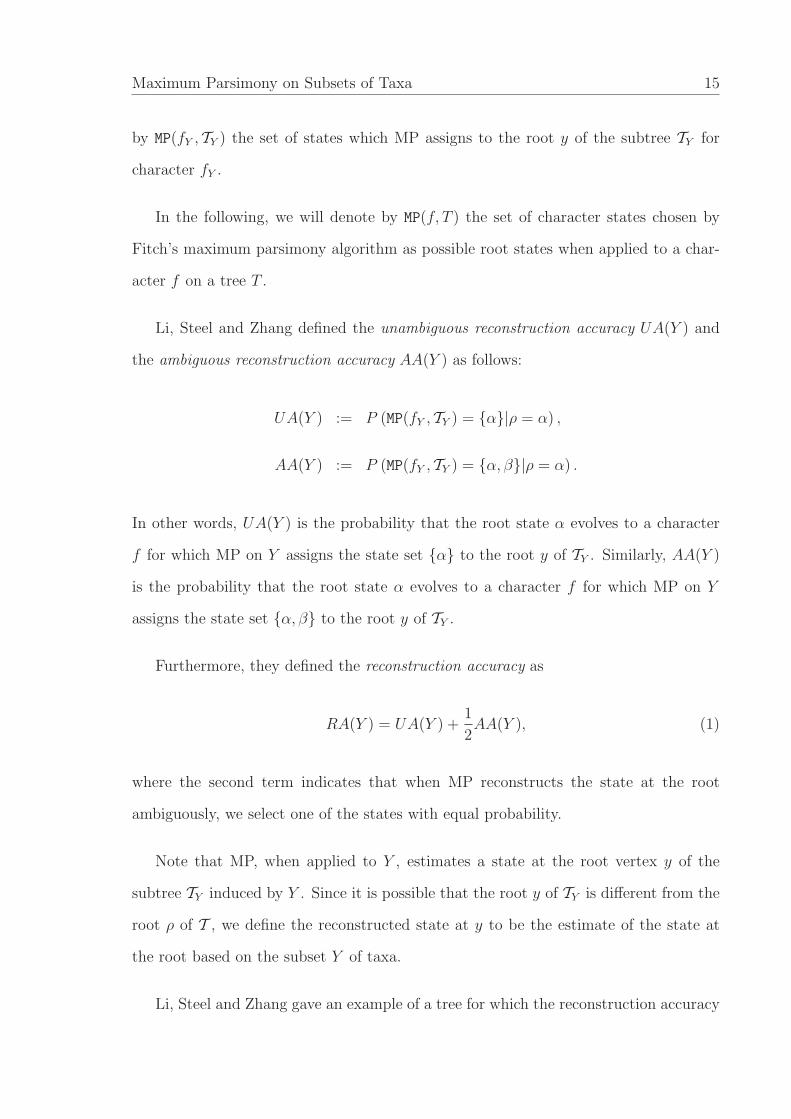
Furthermore, they defined the reconstruction accuracy as
RA(Y ) = UA(Y ) +1
2AA(Y ), (1)
where the second term indicates that when MP reconstructs the state at the root
ambiguously, we select one of the states with equal probability.
Note that MP, when applied to Y , estimates a state at the root vertex y of the
subtree TY induced by Y . Since it is possible that the root y of TY is different from the
root ρ of T , we define the reconstructed state at y to be the estimate of the state at
the root based on the subset Y of taxa.
Li, Steel and Zhang gave an example of a tree for which the reconstruction accuracy
16 Novel Mathematical Aspects of Phylogenetic Estimation
of MP on a proper subset of taxa is higher than the reconstruction accuracy of MP on all
taxa, i.e., RA(Y ) > RA(X) for some proper subset Y of X. But their example requires
that the taxa in Y are closer to the root than the other taxa, i.e., that the probability
of a substitution from the root to any taxon in Y is smaller than the probability of
a substitution from the root to the other taxa. The example that we present in the
following does not require any taxa to be closer to the root. On the contrary, our
example shows that a misleading taxon or taxa (a taxon or taxa that have an adverse
effect on the reconstruction accuracy) may be arbitrarily close to the root.
3.2 An Example of a Misleading Taxon
The main result of this chapter is the following theorem which shows that there are
trees on which the reconstruction accuracy improves when a taxon close to the root is
ignored in an MP based ancestral state reconstruction. Moreover, such a misleading
taxon may be arbitrarily close to the root. Note that we consider a taxon x1 ∈ X to
be closer to the root than a taxon x2 ∈ X whenever the substitution probability from
ρ to x1 is smaller than that from ρ to x2.
Theorem 3.1. Let pz be any real number such that 0 < pz < 12, and assume the N2-
model. Then there exists a binary phylogenetic tree T on a leaf set X and rooted at ρ
such that the following conditions are satisfied:
1. for some leaf z, the substitution probability from ρ to z is pz;
2. RA(X − {z}) > RA(X); and
3. for each leaf v 6= z, the substitution probability pv from ρ to v is more than pz,
i.e., z is closer to the root than any other taxon.
To prove the above theorem, we first need some notation and a lemma. Let y be
a vertex in a binary phylogenetic tree T , and let Y be the set of leaves below y. We
Maximum Parsimony on Subsets of Taxa 17
associate three probabilities with Y as follows.
Pα(Y ) := P (MP(fY , TY ) = {α}|y = α) ,
Pβ(Y ) := P (MP(fY , TY ) = {β}|y = α) ,
Pαβ(Y ) := P (MP(fY , TY ) = {α, β}|y = α) .
Let Th be a balanced binary tree of depth h, i.e., with leaf set X such that |X| = 2h.
Suppose that the substitution probability on each edge of Th is q. For this particu-
lar symmetric tree, we denote Pα(X), Pβ(X) and Pαβ(X) by Pα(h, q), Pβ(h, q) and
Pαβ(h, q), respectively. The convergence properties of these probabilities (for h → ∞
and for various values of q) have been studied in detail, [for example, 40; 48]. We state
the following result on the convergence of Pα(h, q) that additionally provides a lower
bound on Pα(h, q) which is independent of h.
Lemma 3.2 (Charleston and Steel, 1995, Yang, 2008). Let Th be a binary balanced
phylogenetic tree of depth h ≥ 2. Let q < 18
be the probability of a substitution on each
edge of the tree under the N2-model. Then Pα(h, q) approaches
1
2
(
1 − 2q
1 − 2q+
√
(1 − 8q)(1 − 4q)
(1 − 2q)2
)
from above as h → ∞. Moreover, as q goes to 0, the above limiting value approaches 1.
We are now in a position to prove the above theorem.
Proof of Theorem 3.1. Let T be a phylogenetic tree rooted at ρ constructed as follows.
The left subtree of T contains a single leaf z. The right subtree of T is TY with leaf
set Y and root y. Therefore, the leaf set of T is X = Y ∪ {z}. We choose TY to be a
balanced binary tree of depth h and substitution probability q on each edge. Let the
substitution probabilities on (ρ, z) and (ρ, y) be pz and py, respectively, where pz is any
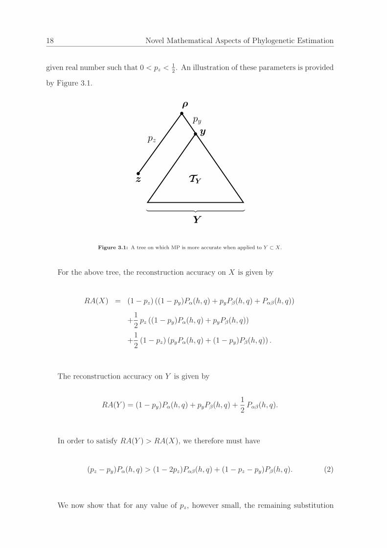
18 Novel Mathematical Aspects of Phylogenetic Estimation
given real number such that 0 < pz < 12. An illustration of these parameters is provided
by Figure 3.1.
︸ ︷︷ ︸
pz
ρ
y
Y
py
z TY
Figure 3.1: A tree on which MP is more accurate when applied to Y ⊂ X.
For the above tree, the reconstruction accuracy on X is given by
RA(X) = (1 − pz) ((1 − py)Pα(h, q) + pyPβ(h, q) + Pαβ(h, q))
+1
2pz ((1 − py)Pα(h, q) + pyPβ(h, q))
+1
2(1 − pz) (pyPα(h, q) + (1 − py)Pβ(h, q)) .
The reconstruction accuracy on Y is given by
RA(Y ) = (1 − py)Pα(h, q) + pyPβ(h, q) +1
2Pαβ(h, q).
In order to satisfy RA(Y ) > RA(X), we therefore must have
(pz − py)Pα(h, q) > (1 − 2pz)Pαβ(h, q) + (1 − pz − py)Pβ(h, q). (2)
We now show that for any value of pz, however small, the remaining substitution
Maximum Parsimony on Subsets of Taxa 19
probabilities q and py and the depth h of TY can be chosen such that RA(Y ) > RA(X)
(Condition 2 in Theorem 3.1), and for every vertex v in Y , the probability of a change
of state from the root to v is more than pz (Condition 3 in Theorem 3.1).
We express the third condition in Theorem 3.1 in a different form. Let Q := 1− 2q,
Pz := 1 − 2pz and Py := 1 − 2py. Since the tree Th is symmetric, the probability of a
change of state from the root to any leaf v in Y is the same, and is given by pv = 1−PyQh
2.
Therefore, the third condition may now be written as PyQh < Pz, or equivalently as
(1 − 2q)h <1 − 2pz
1 − 2py
. (3)
It follows from Lemma 3.2 that, for all h ≥ 2, as q approaches 0, the left hand side
of Equation (2) approaches pz − py and the right hand side approaches 0. Therefore,
there is a real number ǫ such that 0 < ǫ < 18, and whenever q < ǫ, Equation (2) is
satisfied. Now given a value of pz, we first arbitrarily fix py such that 0 < py < pz,
and then fix a value of H := (1 − 2q)h satisfying the constraint in Equation (3). We
then choose h sufficiently large so that q = 12(1 − H
1h ) < ǫ and the constraint given in
Equation (2) is satisfied as well. This completes the proof.
Note that when q ≥ 18, the sequence Pα(h, q) has quite different convergence prop-
erties than when q < 18, and the bound provided by Lemma 3.2 does not apply, [see
40; 48, for details]. Therefore, our construction of a misleading taxon given in the proof
of Theorem 3.1 strongly depends on q being sufficiently small.
3.3 A Single Taxon under a Molecular Clock
In this section, we consider binary characters on a binary phylogenetic tree T with
leaf set X under a molecular clock and the N2-model introduced earlier. Let p be the
probability that a leaf is in a different state than the root. Therefore, if we were to
20 Novel Mathematical Aspects of Phylogenetic Estimation
guess the root state by looking at only one taxon, the probability of success would be
the probability that the root state was conserved at this taxon, which is 1 − p. That
is, if Y = {x1} is a single taxon subset of X, then RA(Y ) = 1− p. In the following, we
show that 1 − p is in fact a lower bound on RA(X), implying that MP applied to all
taxa reconstructs the root state at least as successfully as reconstructing the root state
from a single taxon.
︸ ︷︷ ︸
p1
p′2
p2
p′1
︸ ︷︷ ︸
ρ
y2
y1
Y1 Y2
T2T1
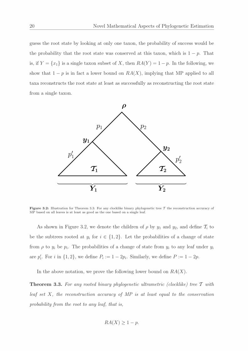
Figure 3.2: Illustration for Theorem 3.3: For any clocklike binary phylogenetic tree T the reconstruction accuracy ofMP based on all leaves is at least as good as the one based on a single leaf.
As shown in Figure 3.2, we denote the children of ρ by y1 and y2, and define Ti to
be the subtrees rooted at yi for i ∈ {1, 2}. Let the probabilities of a change of state
from ρ to yi be pi. The probabilities of a change of state from yi to any leaf under yi
are p′i. For i in {1, 2}, we define Pi := 1 − 2pi. Similarly, we define P := 1 − 2p.
In the above notation, we prove the following lower bound on RA(X).
Theorem 3.3. For any rooted binary phylogenetic ultrametric (clocklike) tree T with
leaf set X, the reconstruction accuracy of MP is at least equal to the conservation
probability from the root to any leaf, that is,
RA(X) ≥ 1 − p.
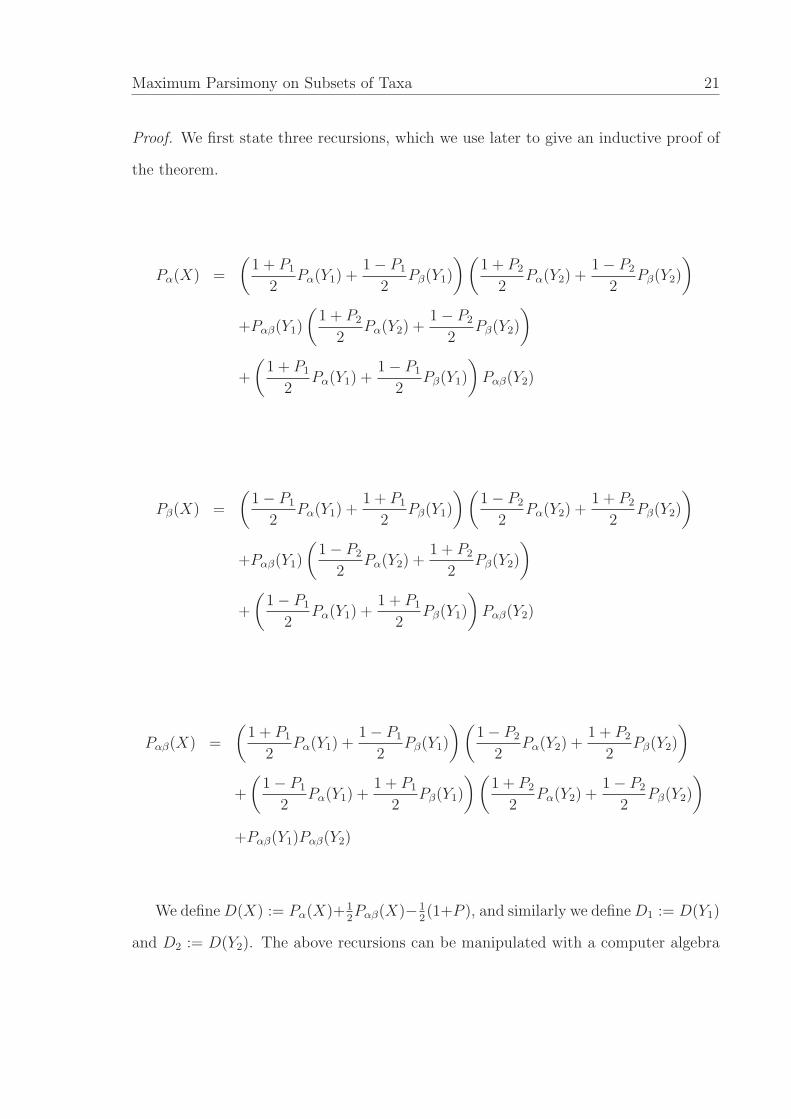
Maximum Parsimony on Subsets of Taxa 21
Proof. We first state three recursions, which we use later to give an inductive proof of
the theorem.
Pα(X) =
(1 + P1
2Pα(Y1) +
1 − P1
2Pβ(Y1)
)(1 + P2
2Pα(Y2) +
1 − P2
2Pβ(Y2)
)
+Pαβ(Y1)
(1 + P2
2Pα(Y2) +
1 − P2
2Pβ(Y2)
)
+
(1 + P1
2Pα(Y1) +
1 − P1
2Pβ(Y1)
)
Pαβ(Y2)
Pβ(X) =
(1 − P1
2Pα(Y1) +
1 + P1
2Pβ(Y1)
)(1 − P2
2Pα(Y2) +
1 + P2
2Pβ(Y2)
)
+Pαβ(Y1)
(1 − P2
2Pα(Y2) +
1 + P2
2Pβ(Y2)
)
+
(1 − P1
2Pα(Y1) +
1 + P1
2Pβ(Y1)
)
Pαβ(Y2)
Pαβ(X) =
(1 + P1
2Pα(Y1) +
1 − P1
2Pβ(Y1)
)(1 − P2
2Pα(Y2) +
1 + P2
2Pβ(Y2)
)
+
(1 − P1
2Pα(Y1) +
1 + P1
2Pβ(Y1)
)(1 + P2
2Pα(Y2) +
1 − P2
2Pβ(Y2)
)
+Pαβ(Y1)Pαβ(Y2)
We define D(X) := Pα(X)+ 12Pαβ(X)− 1
2(1+P ), and similarly we define D1 := D(Y1)
and D2 := D(Y2). The above recursions can be manipulated with a computer algebra
22 Novel Mathematical Aspects of Phylogenetic Estimation
system to verify that
4D(X) = 2Pαβ(Y1)D2P2 + 2Pαβ(Y2)D1P1 + 2D2P2 + 2D1P1 + Pαβ(Y1)P + Pαβ(Y2)P.
Now, by induction on the number of leaves, we show that D(X) is non-negative.
The base case of the inductive proof is when Y1 and Y2 are singleton sets, in which case
D(Y1), D(Y2) and D(X) are all equal to 0, that is RA(X) is 1 − p. Suppose that the
tree T has n taxa, and suppose that D(X) is non-negative for all trees having fewer
than n taxa. Since both Y1 and Y2 contain fewer than n taxa, D(Y1) and D(Y2) are
both non-negative. Since Pαβ(Y1), Pαβ(Y2), P1 and P2 are all non-negative, the right
hand side of the above equation is non-negative, implying the theorem.
3.4 Interpretation
In this chapter, we analyzed the question of how the Fitch MP algorithm performs
when used to reconstruct the ancestral root state. In particular, we considered the
problem for phylogenetic trees on which the probability of a change of state from the
root vertex to any leaf is constant. Earlier simulation studies [e.g., 36; 52] suggested
that the reconstruction accuracy is generally increased when more taxa are considered.
But simulations conducted by Li, Steel and Zhang showed that even under a molecular
clock, MP may perform better on certain subsets of taxa. In Chapter 3.1 we presented
an example of a tree in which one of the subtrees at the root consists of a single leaf
and a pending edge, and the other subtree is a balanced binary tree of depth h, for
some large h, and small (< 18) substitution probabilities on all edges. On this tree, we
observed that the ancestral state reconstruction is more accurate if only the set of taxa
on the balanced subtree is considered. This is in contrast to the example given by Li,
Steel and Zhang in which an outgroup taxon closer to the root or a single fossil record
may give a better estimate of the root state than considering the whole tree. As our
example shows, even a very short edge connecting the root with a leaf cannot guarantee
Maximum Parsimony on Subsets of Taxa 23
an accurate root state estimation if the remaining taxa induce a balanced tree with a
large number of taxa. For such trees, it may be better to ignore the fossil or a taxon
closer to the root. Thus, there seems to be no general theoretical guideline to decide
what subsets of taxa are to be used for a more reliable reconstruction of the root state.
In general, we believe that very long leaf edges would have an adverse effect on the
ancestral state reconstruction using MP.
While using the data on a subset of taxa may give a more accurate estimate of
the root state, in general a single taxon subset does not give a better reconstruction
accuracy. We showed this in Section 3.3 by resolving a conjecture of Li, Steel and Zhang
for the 2-state case. They conjectured that for r-state characters on an ultrametric
(clocklike) tree and a symmetric model of substitution, ancestral state reconstruction
using all taxa is at least as accurate as that using a single taxon. We expect such a
result to be true even when there are more than two states.

24 Novel Mathematical Aspects of Phylogenetic Estimation
Chapter 4
Misleading Sequences
An educated person is one who has learned that information al-
most always turns out to be at best incomplete and very often
false or misleading.
Russell Baker
In the previous chapter, the reconstruction accuracy of Fitch’s MP algorithm for the
estimation of the ancestral root state was analyzed. However, the ever-growing amount
of available genetic sequence data requires stochastic models for nucleotide substitution
and tree reconstruction methods not only to allow for ancestral state reconstructions but
also for the inference of phylogenetic trees. Unsurprisingly, such models and methods
have therefore been widely discussed in the last decades (see, e.g., [10], [12], [38], [50]).
One common method to infer phylogenetic trees is to transform large DNA data sets into
distance matrices, to which distance methods can then be applied. This transformation,
however, inevitably leads to some loss of information, but more seriously, distances
can be positively misleading in extreme cases. Huson and Steel [19] have constructed
sequences yielding a unique most parsimonious tree that is totally different from the tree
univocally supported by the corresponding distances. But their construction required
n− 1 character states for n taxa and therefore cannot be realized with DNA sequences
whenever n > 5.
We will show here that no more than three states are actually needed, that is, binary
and ternary characters suffice for generating the extreme contrast between parsimony-
and distance-based trees. We do this in a constructive way, i.e., for any choice of
binary phylogenetic trees T1, T2, we show how to generate a sequence of binary and
ternary characters for which T1 is the unique MP-tree and T2 is the best possible tree
25
26 Novel Mathematical Aspects of Phylogenetic Estimation
concerning the induced distances. For this purpose, parsimoniously non-informative
characters are very useful because they can yield some signal for distance-based methods
but do not discriminate between trees under the parsimony criterion. Specifically,
not only can non-informative ternary characters jointly generate any non-trivial split
metric (along with some trivial split metrics), they can totally cancel any non-trivial
split metric (i.e., generate a star tree), too. We can thus freely navigate between
perfectly additive distances by using only non-informative ternary characters. Last but
not least, we compare the sequence length of our construction to that of the Huson-
Steel construction and show that our sequences can be significantly shorter. We then
introduce an approach on how to characterize all misleading sequences for the four taxa
case. Finally, we analyze the relevance of misleading sequences for practical purposes
and show a misleading example from a DNA alignment including a human gene.
4.1 Construction of Misleading Sequences from Ternary Characters
We begin with some notation. In the following, we will assume that X is a set of n ≥ 4
taxa.
Let df : X × X → N denote the Hamming distance induced by a character f and
dS :=k∑
i=1
dfifor sequences S = f1...fk of k characters. Note that since df only depends
on the partitions associated with the character f , we may index d by the corresponding
partitions instead. In the case of a k-ary character f , which partitions the taxon set
into k parts A1, . . . , Ak, we also denote the Hamming distance as dA1|...|Ak:= df .
Recall that a non-informative ternary character f has three character states α, β,
γ for which α and β are attained in X exactly once: f(a) = α, f(b) = β, and f(x) = γ
for all taxa a, b, and x different from a and b. Such a character on X featuring the two
taxa a, b thus induces a ‘trivial’ partition of X into two singletons and a remainder, for
which we use the shorthand a|b|X−a, b. Similarly, the ‘trivial’ partition (alias trivial
split) of X associated with a non-informative binary character distinguishing taxon a
Misleading Sequences 27
is denoted by a|X−a.
We now give a formal definition of misleading sequences and distances, before we
continue with some more preliminaries required to prove Theorem 4.4, which is the
main result of this chapter.
Definition 4.1. A sequence S of characters on a leaf set X, which is convex only on
a binary phylogenetic X-tree T1 and whose derived Hamming distances are additive on
a binary phylogenetic X-tree T2 such that T1 6= T2, is called a misleading sequence, and
its derived Hamming distances dS are called misleading distances.
We now explore some useful properties of the Hamming distance which are needed
as prerequisites to construct misleading sequences from binary and ternary characters.
First, note that the mismatch distances derived from a partition with k parts
A1, . . . , Ak cannot be distinguished from the sum of the mismatch distances derived
from the half-weighted splits Ai|X−Ai (i = 1, . . . , k):
dA1|...|Ak=
1
2
(dA1|X−A1 + . . . + dAk|X−Ak
). (4)
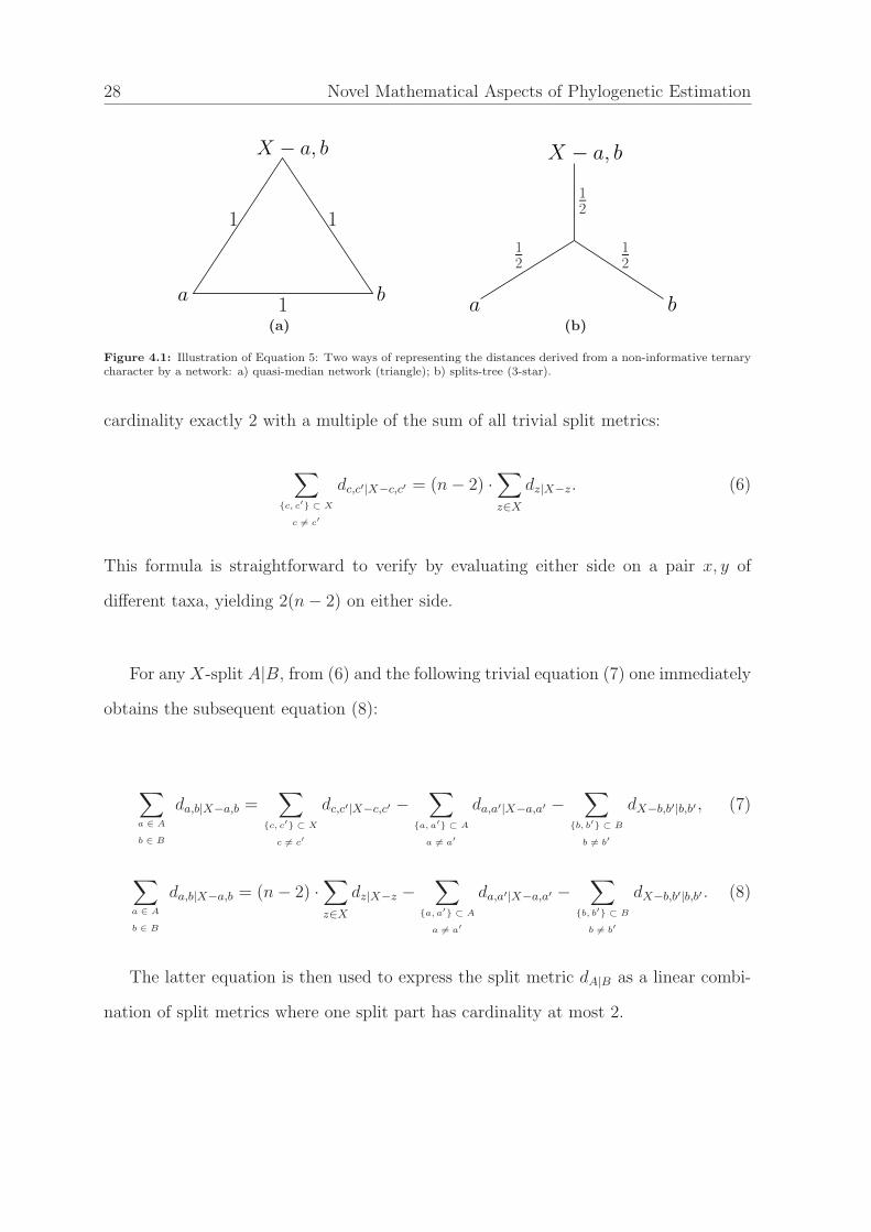
In particular, if f is a non-informative ternary character featuring the two taxa
a, b, then the derived mismatch distance df = da|b|X−a,b equals the sum of the three
mismatch distances derived from the half-weighted splits a|X−a, b|X−b, and a,b|X−a,b:
da|b|X−a,b =1
2
(da|X−a + db|X−b + da,b|X−a,b
). (5)
This obvious relationship is illustrated in Figure 4.1. This representation thus per-
mits substituting da|b|X−a,b by da,b|X−a,b, or vice versa, modulo trivial split metrics.
Linear dependence of the split metrics on X leads to several equations; for instance,
the most fundamental one equates the sum of all split metrics where one part has
28 Novel Mathematical Aspects of Phylogenetic Estimation
a
X − a, b
b
1 1
1
(a)
a b
1
2
1
2
1
2
X − a, b
(b)
Figure 4.1: Illustration of Equation 5: Two ways of representing the distances derived from a non-informative ternarycharacter by a network: a) quasi-median network (triangle); b) splits-tree (3-star).
cardinality exactly 2 with a multiple of the sum of all trivial split metrics:
∑
{c, c′} ⊂ X
c 6= c′
dc,c′|X−c,c′ = (n − 2) ·∑
z∈X
dz|X−z. (6)
This formula is straightforward to verify by evaluating either side on a pair x, y of
different taxa, yielding 2(n − 2) on either side.
For any X-split A|B, from (6) and the following trivial equation (7) one immediately
obtains the subsequent equation (8):
∑
a ∈ A
b ∈ B
da,b|X−a,b =∑
{c, c′} ⊂ X
c 6= c′
dc,c′|X−c,c′ −∑
{a, a′} ⊂ A
a 6= a′
da,a′|X−a,a′ −∑
{b, b′} ⊂ B
b 6= b′
dX−b,b′|b,b′ , (7)
∑
a ∈ A
b ∈ B
da,b|X−a,b = (n − 2) ·∑
z∈X
dz|X−z −∑
{a, a′} ⊂ A
a 6= a′
da,a′|X−a,a′ −∑
{b, b′} ⊂ B
b 6= b′
dX−b,b′|b,b′ . (8)
The latter equation is then used to express the split metric dA|B as a linear combi-
nation of split metrics where one split part has cardinality at most 2.
Misleading Sequences 29
Lemma 4.2. The split metric dA|B for a non-trivial split A|B of an n-taxa set X
satisfies the following two equations:
dA|B =1
2
|B|∑
a∈A
da|X−a + |A|∑
b∈B
dX−b|b −∑
a ∈ A
b ∈ B
da,b|X−a,b
, (9)
dA|B =1
2
∑
{a, a′} ⊂ A
a 6= a′
da,a′|X−a,a′ +∑
{b, b′} ⊂ B
b 6= b′
dX−b,b′|b,b′ − (|A| − 2)∑
a∈A
da|X−a − (|B| − 2)∑
b∈B
dX−b|b
.
(10)
Proof. To prove (9), one needs to evaluate either side on a pair x, y where x is from A,
say, and y is either from A−x or from B. The result on the right side is 12[2·|B|−2·|B|] =
0 in the former case and equal to 12[|B|+ |A|−(n−2)] = 1 in the latter case, as required.
From (9) one readily derives (10) by substituting the sum of all da,b|X−a,b (a ∈ A, b ∈ B)
by the right-hand side of (8).
This lemma and the preceding equations constitute the ingredients for the following
proposition, which describes how one can either cancel or create a single split metric
by means of metrics derived from non-informative ternary characters.
Proposition 4.3. The split metric dA|B for a non-trivial split A|B of an n-taxa set
X can, up to a sum of trivial split metrics, either be canceled via
dA|B +∑
a ∈ A
b ∈ B
da|b|X−a,b = |B|∑
a∈A
da|X−a + |A|∑
b∈B
db|X−b, (11)
or be created via
∑
{a, a′} ⊂ A
a 6= a′
da|a′|X−a,a′+∑
{b, b′} ⊂ B
b 6= b′
dX−b,b′|b|b′ = dA|B+
(
|A| − 3
2
)∑
a∈A
da|X−a+
(
|B| − 3
2
)∑
b∈B
db|X−b
(12)
through metrics derived from non-informative ternary characters.
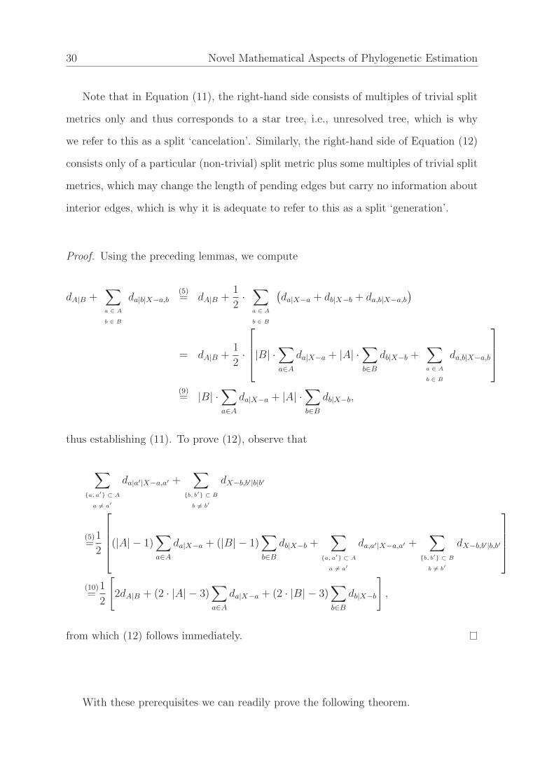
30 Novel Mathematical Aspects of Phylogenetic Estimation
Note that in Equation (11), the right-hand side consists of multiples of trivial split
metrics only and thus corresponds to a star tree, i.e., unresolved tree, which is why
we refer to this as a split ‘cancelation’. Similarly, the right-hand side of Equation (12)
consists only of a particular (non-trivial) split metric plus some multiples of trivial split
metrics, which may change the length of pending edges but carry no information about
interior edges, which is why it is adequate to refer to this as a split ‘generation’.
Proof. Using the preceding lemmas, we compute
dA|B +∑
a ∈ A
b ∈ B
da|b|X−a,b(5)= dA|B +
1
2·∑
a ∈ A
b ∈ B
(da|X−a + db|X−b + da,b|X−a,b
)
= dA|B +1
2·
|B| ·
∑
a∈A
da|X−a + |A| ·∑
b∈B
db|X−b +∑
a ∈ A
b ∈ B
da,b|X−a,b
(9)= |B| ·
∑
a∈A
da|X−a + |A| ·∑
b∈B
db|X−b,
thus establishing (11). To prove (12), observe that
∑
{a, a′} ⊂ A
a 6= a′
da|a′|X−a,a′ +∑
{b, b′} ⊂ B
b 6= b′
dX−b,b′|b|b′
(5)=
1
2
(|A| − 1)∑
a∈A
da|X−a + (|B| − 1)∑
b∈B
db|X−b +∑
{a, a′} ⊂ A
a 6= a′
da,a′|X−a,a′ +∑
{b, b′} ⊂ B
b 6= b′
dX−b,b′|b,b′
(10)=
1
2
[
2dA|B + (2 · |A| − 3)∑
a∈A
da|X−a + (2 · |B| − 3)∑
b∈B
db|X−b
]
,
from which (12) follows immediately.
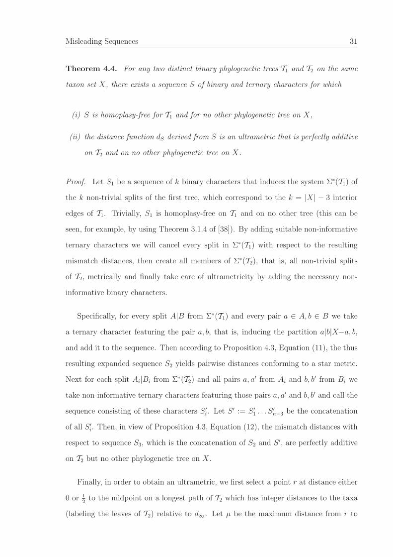
With these prerequisites we can readily prove the following theorem.
Misleading Sequences 31
Theorem 4.4. For any two distinct binary phylogenetic trees T1 and T2 on the same
taxon set X, there exists a sequence S of binary and ternary characters for which
(i) S is homoplasy-free for T1 and for no other phylogenetic tree on X,
(ii) the distance function dS derived from S is an ultrametric that is perfectly additive
on T2 and on no other phylogenetic tree on X.
Proof. Let S1 be a sequence of k binary characters that induces the system Σ∗(T1) of
the k non-trivial splits of the first tree, which correspond to the k = |X| − 3 interior
edges of T1. Trivially, S1 is homoplasy-free on T1 and on no other tree (this can be
seen, for example, by using Theorem 3.1.4 of [38]). By adding suitable non-informative
ternary characters we will cancel every split in Σ∗(T1) with respect to the resulting
mismatch distances, then create all members of Σ∗(T2), that is, all non-trivial splits
of T2, metrically and finally take care of ultrametricity by adding the necessary non-
informative binary characters.
Specifically, for every split A|B from Σ∗(T1) and every pair a ∈ A, b ∈ B we take
a ternary character featuring the pair a, b, that is, inducing the partition a|b|X−a, b,
and add it to the sequence. Then according to Proposition 4.3, Equation (11), the thus
resulting expanded sequence S2 yields pairwise distances conforming to a star metric.
Next for each split Ai|Bi from Σ∗(T2) and all pairs a, a′ from Ai and b, b′ from Bi we
take non-informative ternary characters featuring those pairs a, a′ and b, b′ and call the
sequence consisting of these characters S ′i. Let S ′ := S ′
1 . . . S ′n−3 be the concatenation
of all S ′i. Then, in view of Proposition 4.3, Equation (12), the mismatch distances with
respect to sequence S3, which is the concatenation of S2 and S ′, are perfectly additive
on T2 but no other phylogenetic tree on X.
Finally, in order to obtain an ultrametric, we first select a point r at distance either
0 or 12
to the midpoint on a longest path of T2 which has integer distances to the taxa
(labeling the leaves of T2) relative to dS3 . Let µ be the maximum distance from r to
32 Novel Mathematical Aspects of Phylogenetic Estimation
a taxon in X. Then, for every x ∈ X, add µ − dS3(r, x) many non-informative binary
characters featuring x to the current sequence S3. Then the final sequence S delivers
an ultrametric dS and still supports T2 and only T2, as required. This finishes the proof
of the Theorem.
We will now illustrate our construction with the help of an example.
4.1.1 Illustration
1 : α α α α α γ γ γ α α γ γ γ γ α γ γ γ α α γ γ β
2 : α α γ γ γ α α α γ γ α α γ γ γ α α γ γ γ γ α β
3 : β α β γ γ β γ γ γ γ γ γ α α β γ γ γ β γ α γ α
4 : β β γ β γ γ β γ β γ β γ β γ γ β γ α γ β β γ β
5 : β β γ γ β γ γ β γ β γ β γ β γ γ β β γ γ γ β β
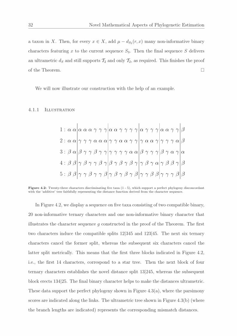
Figure 4.2: Twenty-three characters discriminating five taxa (1 - 5), which support a perfect phylogeny disconcordantwith the ‘additive’ tree faithfully representing the distance function derived from the character sequence.
In Figure 4.2, we display a sequence on five taxa consisting of two compatible binary,
20 non-informative ternary characters and one non-informative binary character that
illustrates the character sequence g constructed in the proof of the Theorem. The first
two characters induce the compatible splits 12|345 and 123|45. The next six ternary
characters cancel the former split, whereas the subsequent six characters cancel the
latter split metrically. This means that the first three blocks indicated in Figure 4.2,
i.e., the first 14 characters, correspond to a star tree. Then the next block of four
ternary characters establishes the novel distance split 13|245, whereas the subsequent
block erects 134|25. The final binary character helps to make the distances ultrametric.
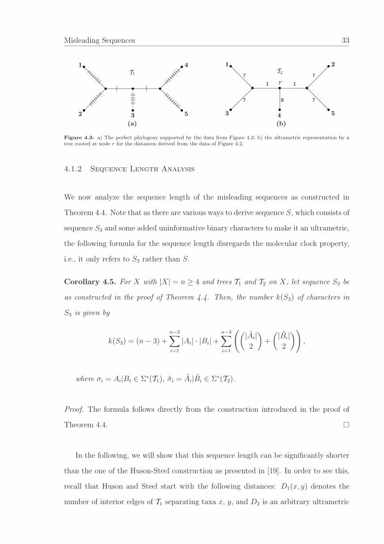
These data support the perfect phylogeny shown in Figure 4.3(a), where the parsimony
scores are indicated along the links. The ultrametric tree shown in Figure 4.3(b) (where
the branch lengths are indicated) represents the corresponding mismatch distances.
Misleading Sequences 33
3
T1
41
2 5
(a)
7
1
7
8
1
7
7
4
T2
21
3 5
r
(b)
Figure 4.3: a) The perfect phylogeny supported by the data from Figure 4.2; b) the ultrametric representation by atree rooted at node r for the distances derived from the data of Figure 4.2.
4.1.2 Sequence Length Analysis
We now analyze the sequence length of the misleading sequences as constructed in
Theorem 4.4. Note that as there are various ways to derive sequence S, which consists of
sequence S3 and some added uninformative binary characters to make it an ultrametric,
the following formula for the sequence length disregards the molecular clock property,
i.e., it only refers to S3 rather than S.
Corollary 4.5. For X with |X| = n ≥ 4 and trees T1 and T2 on X, let sequence S3 be
as constructed in the proof of Theorem 4.4. Then, the number k(S3) of characters in
S3 is given by
k(S3) = (n − 3) +n−3∑
i=1
|Ai| · |Bi| +n−3∑
i=1
((|Ai|2
)
+
(|Bi|2
))
,
where σi = Ai|Bi ∈ Σ∗(T1), σi = Ai|Bi ∈ Σ∗(T2).
Proof. The formula follows directly from the construction introduced in the proof of
Theorem 4.4.
In the following, we will show that this sequence length can be significantly shorter
than the one of the Huson-Steel construction as presented in [19]. In order to see this,
recall that Huson and Steel start with the following distances: D1(x, y) denotes the
number of interior edges of T1 separating taxa x, y, and D2 is an arbitrary ultrametric
34 Novel Mathematical Aspects of Phylogenetic Estimation
on T2 such that all interior edges have edge weight 1 and all pending edges have a
non-negative integer edge weight. Moreover, they set dij := |D2(i, j) − D1(i, j)|, s =∑
i∈X
∑
j 6=i∈X
dij. Finally, they define nij = r − B · dij + s, where B =((
n2
)− 1)
and r is
such that r − dij + s ≥ 0 for all dij.
Note that this construction does not lead to a unique sequence as there are various
choices of D2, which lead to different sequences and different edge lengths. The basic
approach used by Huson and Steel is this: they first add B copies of all binary characters
induced by the n−3 interior edges of T1, i.e., by Σ∗(T1), and then they concatenate this
sequence with nij copies of a character in which the (distinct) taxa i and j are in state α,
and all other taxa are in states other than α and different from one another. The latter
characters are all non-informative. So as in our approach, non-informative characters
are used to cancel splits induced by the binary characters defining the perfect phylogeny.
But the non-informative characters of the Huson-Steel approach employ n−1 character
states (where n = |X|) as opposed to the three states required by the Bandelt-Fischer
approach.
Concerning the sequence length of the Huson-Steel construction, we can now state
the following lemma.
Lemma 4.6. The number of characters k(S) of the misleading sequence S constructed
in [19] is
k(S) =
((n
2
)
− 1
)
(n − 3) +∑
i∈X
∑
j 6=i∈X
nij. (13)
In order to compare k(S3) and k(S), we have to make sure that we do not make
k(S) unnecessarily large. Note that as soon as D2 is chosen, the values for dij and s
are fixed. So one can only minimize∑
nij by making r minimal. This means that r
has to be chosen such that r = B · maxij dij − s. Let d∗ij = maxij dij.
Misleading Sequences 35
Lemma 4.7. The number of characters k(S) of the misleading sequence S constructed
in [19] is bounded from below by
k(S) ≥((
n
2
)
− 1
)
·(
(n − 3) +
(n
2
)
· d∗ij − s
)
.
Proof. From Lemma 4.6 we have
k(S) =
((n
2
)
− 1
)
(n − 3) +∑
i∈X
∑
j 6=i∈X
(r − B · dij + s)
=
((n
2
)
− 1
)
(n − 3) +
(n
2
)
(r + s) − B ·∑
i∈X
∑
j 6=i∈X
dij
=
((n
2
)
− 1
)
(n − 3) +
(n
2
)
(r + s) − B · s
≥((
n
2
)
− 1
)
(n − 3) +
((n
2
)
− 1
)
·((
n
2
)
· d∗ij − s
)
=
((n
2
)
− 1
)
·(
(n − 3) +
(n
2
)
· d∗ij − s
)
,
where the lower bound in the second to last step is obtained by using the the minimal
value for r, i.e., r = B · d∗ij − s.
Even the lower bound on the sequence length of S is not independent of the original
choice of D2. Therefore, the sequence lengths of the Huson-Steel approach and the
Bandelt-Fischer approach cannot directly be compared. However, we will show with
the following example that the difference can in fact be huge.
Example 4.8. Consider again trees T1 and T2 given by Figure 4.3. We will now follow
the Huson-Steel approach for these trees, and we will also use D2 as given in Figure
4.3.
Table 2 shows the values required for the Huson-Steel approach. Note that here,
r is chosen to be minimal. Since B =(52
)− 1 = 9 by definition, and since s = 144
36 Novel Mathematical Aspects of Phylogenetic Estimation
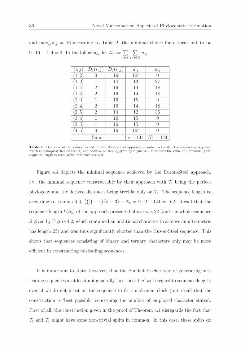
and maxij dij = 16 according to Table 2, the minimal choice for r turns out to be
9 · 16 − 144 = 0. In the following, let Nr :=∑
i∈X
∑
j 6=i∈X
nij.
(i, j) D1(i, j) D2(i, j) dij nij
(1, 2) 0 16 16∗ 0(1, 3) 1 14 13 27(1, 4) 2 16 14 18(1, 5) 2 16 14 18(2, 3) 1 16 15 9(2, 4) 2 16 14 18(2, 5) 2 14 12 36(3, 4) 1 16 15 9(3, 5) 1 16 15 9(4, 5) 0 16 16∗ 0
Sum: s = 144 N0 = 144
Table 2: Overview of the values needed for the Huson-Steel approach in order to construct a misleading sequencewhich is homoplasy-free on tree T1 and additive on tree T2 given by Figure 4.3. Note that the value of r minimizing thesequence length is used, which here means r = 0.
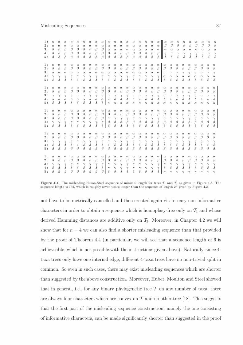
Figure 4.4 depicts the minimal sequence achieved by the Huson-Steel approach,
i.e., the minimal sequence constructable by their approach with T1 being the perfect
phylogeny and the derived distances being treelike only on T2. The sequence length is,
according to Lemma 4.6,((
52
)− 1)(5 − 3) + Nr = 9 · 2 + 144 = 162. Recall that the
sequence length k(S3) of the approach presented above was 22 (and the whole sequence
S given by Figure 4.2, which contained an additional character to achieve an ultrametric
has length 23) and was thus significantly shorter than the Huson-Steel sequence. This
shows that sequences consisting of binary and ternary characters only may be more
efficient in constructing misleading sequences.
It is important to state, however, that the Bandelt-Fischer way of generating mis-
leading sequences is at least not generally ‘best possible’ with regard to sequence length,
even if we do not insist on the sequence to fit a molecular clock (but recall that the
construction is ‘best possible’ concerning the number of employed character states).
First of all, the construction given in the proof of Theorem 4.4 disregards the fact that
T1 and T2 might have some non-trivial splits in common. In this case, these splits do
Misleading Sequences 37
1 : α2 : α3 : β4 : β5 : β
ααβββ
ααβββ
ααβββ
ααβββ
ααβββ
ααβββ
ααβββ
ααβββ
αααββ
αααββ
αααββ
αααββ
αααββ
αααββ
αααββ
αααββ
αααββ
αβαγδ
αβαγδ
αβαγδ
αβαγδ
αβαγδ
αβαγδ
αβαγδ
αβαγδ
αβαγδ
1 : α2 : β3 : α4 : γ5 : δ
αβαγδ
αβαγδ
αβαγδ
αβαγδ
αβαγδ
αβαγδ
αβαγδ
αβαγδ
αβαγδ
αβαγδ
αβαγδ
αβαγδ
αβαγδ
αβαγδ
αβαγδ
αβαγδ
αβαγδ
αβγαδ
αβγαδ
αβγαδ
αβγαδ
αβγαδ
αβγαδ
αβγαδ
αβγαδ
αβγαδ
1 : α2 : β3 : γ4 : α5 : δ
αβγαδ
αβγαδ
αβγαδ
αβγαδ
αβγαδ
αβγαδ
αβγαδ
αβγαδ
αβγδα
αβγδα
αβγδα
αβγδα
αβγδα
αβγδα
αβγδα
αβγδα
αβγδα
αβγδα
αβγδα
αβγδα
αβγδα
αβγδα
αβγδα
αβγδα
αβγδα
αβγδα
1 : α2 : β3 : β4 : γ5 : δ
αββγδ
αββγδ
αββγδ
αββγδ
αββγδ
αββγδ
αββγδ
αββγδ
αβγβδ
αβγβδ
αβγβδ
αβγβδ
αβγβδ
αβγβδ
αβγβδ
αβγβδ
αβγβδ
αβγβδ
αβγβδ
αβγβδ
αβγβδ
αβγβδ
αβγβδ
αβγβδ
αβγβδ
αβγβδ
1 : α2 : β3 : γ4 : δ5 : β
αβγδβ
αβγδβ
αβγδβ
αβγδβ
αβγδβ
αβγδβ
αβγδβ
αβγδβ
αβγδβ
αβγδβ
αβγδβ
αβγδβ
αβγδβ
αβγδβ
αβγδβ
αβγδβ
αβγδβ
αβγδβ
αβγδβ
αβγδβ
αβγδβ
αβγδβ
αβγδβ
αβγδβ
αβγδβ
αβγδβ
1 : α2 : β3 : γ4 : δ5 : β
αβγδβ
αβγδβ
αβγδβ
αβγδβ
αβγδβ
αβγδβ
αβγδβ
αβγδβ
αβγγδ
αβγγδ
αβγγδ
αβγγδ
αβγγδ
αβγγδ
αβγγδ
αβγγδ
αβγγδ
αβγδγ
αβγδγ
αβγδγ
αβγδγ
αβγδγ
αβγδγ
αβγδγ
αβγδγ
αβγδγ
Figure 4.4: The misleading Huson-Steel sequence of minimal length for trees T1 and T2 as given in Figure 4.3. Thesequence length is 162, which is roughly seven times longer than the sequence of length 23 given by Figure 4.2.
not have to be metrically cancelled and then created again via ternary non-informative
characters in order to obtain a sequence which is homoplasy-free only on T1 and whose
derived Hamming distances are additive only on T2. Moreover, in Chapter 4.2 we will
show that for n = 4 we can also find a shorter misleading sequence than that provided
by the proof of Theorem 4.4 (in particular, we will see that a sequence length of 6 is
achieveable, which is not possible with the instructions given above). Naturally, since 4-
taxa trees only have one internal edge, different 4-taxa trees have no non-trivial split in
common. So even in such cases, there may exist misleading sequences which are shorter
than suggested by the above construction. Moreover, Huber, Moulton and Steel showed
that in general, i.e., for any binary phylogenetic tree T on any number of taxa, there
are always four characters which are convex on T and no other tree [18]. This suggests
that the first part of the misleading sequence construction, namely the one consisting
of informative characters, can be made significantly shorter than suggested in the proof
38 Novel Mathematical Aspects of Phylogenetic Estimation
pattern character type corresponding variable
1 : ααββ binary, informative x1
2 : αβββ binary, non-informative x2
3 : αβαα binary, non-informative x3
4 : ααβα binary, non-informative x4
5 : αααβ binary, non-informative x5
6 : ααβγ ternary, non-informative x6
7 : αβαγ ternary, non-informative x7
8 : αβγα ternary, non-informative x8
9 : αββγ ternary, non-informative x9
10 : αβγβ ternary, non-informative x10
11 : αγββ ternary, non-informative x11
12 : αβαβ binary, informative x12
13 : αββα binary, informative x13
14 : αβγδ quaternary, non-informative x14
15 : αααα unitary, non-informative x15
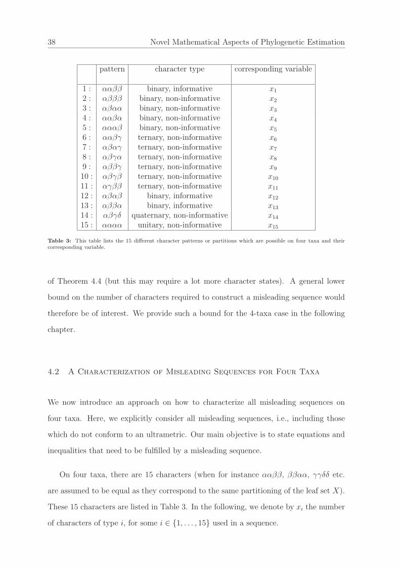
Table 3: This table lists the 15 different character patterns or partitions which are possible on four taxa and theircorresponding variable.
of Theorem 4.4 (but this may require a lot more character states). A general lower
bound on the number of characters required to construct a misleading sequence would
therefore be of interest. We provide such a bound for the 4-taxa case in the following
chapter.
4.2 A Characterization of Misleading Sequences for Four Taxa
We now introduce an approach on how to characterize all misleading sequences on
four taxa. Here, we explicitly consider all misleading sequences, i.e., including those
which do not conform to an ultrametric. Our main objective is to state equations and
inequalities that need to be fulfilled by a misleading sequence.
On four taxa, there are 15 characters (when for instance ααββ, ββαα, γγδδ etc.
are assumed to be equal as they correspond to the same partitioning of the leaf set X).
These 15 characters are listed in Table 3. In the following, we denote by xi the number
of characters of type i, for some i ∈ {1, . . . , 15} used in a sequence.
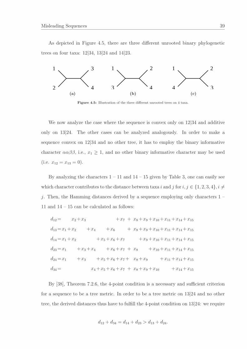
Misleading Sequences 39
As depicted in Figure 4.5, there are three different unrooted binary phylogenetic
trees on four taxa: 12|34, 13|24 and 14|23.
3
42
1
(a)
2
43
1
(b)
2
34
1
(c)
Figure 4.5: Illustration of the three different unrooted trees on 4 taxa.
We now analyze the case where the sequence is convex only on 12|34 and additive
only on 13|24. The other cases can be analyzed analogously. In order to make a
sequence convex on 12|34 and no other tree, it has to employ the binary informative
character ααββ, i.e., x1 ≥ 1, and no other binary informative character may be used
(i.e. x12 = x13 = 0).
By analyzing the characters 1 – 11 and 14 – 15 given by Table 3, one can easily see
which character contributes to the distance between taxa i and j for i, j ∈ {1, 2, 3, 4}, i 6=
j. Then, the Hamming distances derived by a sequence employing only characters 1 –
11 and 14 – 15 can be calculated as follows:
d12 = x2 +x3 +x7 + x8 +x9 +x10 +x11 +x14 +x15
d13 =x1 +x2 +x4 +x6 + x8 +x9 +x10 +x11 +x14 +x15
d14 =x1 +x2 +x5 +x6 +x7 +x9 +x10 +x11 +x14 +x15
d23 =x1 +x3 +x4 +x6 +x7 + x8 +x10 +x11 +x14 +x15
d24 =x1 +x3 +x5 +x6 +x7 + x8 +x9 +x11 +x14 +x15
d34 = x4 +x5 +x6 +x7 + x8 +x9 +x10 +x14 +x15
By [38], Theorem 7.2.6, the 4-point condition is a necessary and sufficient criterion
for a sequence to be a tree metric. In order to be a tree metric on 13|24 and no other
tree, the derived distances thus have to fulfill the 4-point condition on 13|24: we require
d12 + d34 = d14 + d23 > d13 + d24.

40 Novel Mathematical Aspects of Phylogenetic Estimation
Note that in order to avoid a star tree, the last inequality has to be strict. Furthermore,
we require all triangle inequalities to hold (note that these are induced by the general
form of the 4-point condition as the four points need not be all distinct):
dij + djk − dik ≥ 0 for all i, j, k ∈ {1, 2, 3, 4}.
So altogether we have the following conditions on d to make it a tree metric (exclusively)
on 13|24:
d12 + d34 = d14 + d23 > d13 + d24 (14)
d12 + d23 ≥ d13 (15)
d13 + d23 ≥ d12 (16)
d12 + d13 ≥ d23 (17)
d12 + d24 ≥ d14 (18)
d14 + d24 ≥ d12 (19)
d12 + d14 ≥ d24 (20)
d13 + d34 ≥ d14 (21)
d14 + d34 ≥ d13 (22)
d13 + d14 ≥ d34 (23)
d23 + d34 ≥ d24 (24)
d24 + d34 ≥ d23 (25)
d23 + d24 ≥ d34 (26)
This leads directly to the following corollary.
Corollary 4.9. Any choice of x1, . . . , x15 with x1 ≥ 1 and x12 = x13 = 0 such that
Inequalities (14) – (26) are fulfilled induces a misleading sequence S on four taxa.
More precisely, S is homoplasy-free only on tree 12|34 and additive only on tree 13|24.
Moreover, for any sequence S which is homoplasy-free only on tree 12|34 and additive
only on tree 13|24 we have x1 ≥ 1 and x12 = x13 = 0. Additionally, such a sequence
fulfills Inequalities (14) – (26).
Misleading Sequences 41
Proof. The claim follows directly from the preceding arguments.
Remark: Note that the roles of the trees can be swapped by modifying the inequali-
ties accordingly. Thus, a full characterization of all misleading sequences on 4 taxa can
be achieved with this approach.
We are now in the position to prove a lower bound for the sequence length required
to construct misleading sequences on four taxa.
Proposition 4.10. Let T1 and T2 be two distinct binary phylogenetic X-trees, where
|X| = 4. Then, any sequence S of characters on X such that
1. T1 is the unique MP-tree and
2. the Hamming distances derived from S are perfectly additive on T2
has length at least six.
Proof. We assume wlog. that T1 = 12|34 and T2 = 13|24. Then, we know that in
order for T1 to be the unique MP-tree, we require x12 = x13 = 0. Note that the
unitary non-informative character αααα and the quaternary non-informative character
αβγδ are not only non-informative regarding parsimony, but also regarding distances.
Therefore, in order to determine the minimum length of a misleading sequence S, we
can furthermore assume wlog. x14 = x15 = 0. Then, by Inequality (14), we need
d12 + d34 = d14 + d23 > d13 + d24. As above we can express the distances as follows:
1. d12 + d34 = x2 + x3 + x4 + x5 + x6 + 2x7 + 2x8 + 2x9 + 2x10
2. d14 + d23 = 2x1 + x2 + x4 + x5 + 2x6 + 2x7 + x8 + x9 + 2x10 + 2x11
3. d13 + d24 = 2x1 + x2 + x3 + x4 + x5 + 2x6 + x7 + 2x8 + 2x9 + x10 + 2x11
42 Novel Mathematical Aspects of Phylogenetic Estimation
This leads to x7+x10 > x8+x9 = 2x1+x6+2x11. As x1 ≥ 1 as T1 is the unique MP-tree,
this means that x8+x9 ≥ 2 and x7+x10 ≥ 3. Therefore, we have x1+x7+x8+x9+x10 ≥
6. This completes the proof.
Corollary 4.11. Let S be a misleading sequence on |X| = n ≥ 4 taxa, such that S
contains all binary characters induced by the non-trivial splits of its perfect phylogeny.
Then, S has length at least six. Moreover, the function f : N → N defined by n 7→
minS length(S), which maps the number of taxa to the minimum length of misleading
sequences on n taxa with the additional property of containing all binary characters
induced by the non-trivial splits of their perfect phylogeny, is non-decreasing.
Proof. We will prove the claim by induction on n = |X|. For |X| = 4, the result
follows from Proposition 4.10. Now let n be a number of taxa such that for misleading
sequences (with the additional property of containing all binary characters induced
by the non-trivial splits of their perfect phylogeny) on fewer than n taxa we already
know that they have at least length k for some k ≥ 6, and that f(i) is non-decreasing
over the range i = 4, . . . , n − 1. Let S be a character sequence which has T1 as its
unique perfect phylogeny and which contains all n− 3 binary characters induced by its
non-trivial splits and whose derived Hamming distances are treelike only on T2, where
T1 6= T2 are X-trees with |X| = n. Let additionally the length of S be f(n) (i.e., S is a
misleading sequence containing all binary characters induced by splits of T1 of minimum
length). Now for an arbitrary taxon x ∈ X, we consider Sx := S|X−{x}, T x1 := T1|X−{x}
and T x2 := T2|X−{x}, i.e., the restrictions of S, T1 and T2 on X − {x}, respectively.
Note that Sx is convex on T x1 . This is due to the fact that the removal of a row in
the alignment S cannot create homoplasies as some informative characters may become
non-informative, but non-informative characters remain non-informative. Therefore, no
conflicting signals are added. Furthermore, note that the Hamming distances derived
from Sx are additive on T x2 , as deleting a row of S cannot destroy additivity: since
the distances derived by S fit on T2, by disregarding x we do not change the fact that
the remaining distances fit on the remaining edges. Now, S contains by assumption
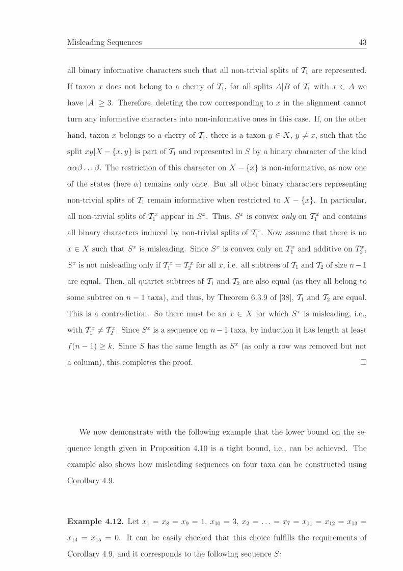
Misleading Sequences 43
all binary informative characters such that all non-trivial splits of T1 are represented.
If taxon x does not belong to a cherry of T1, for all splits A|B of T1 with x ∈ A we
have |A| ≥ 3. Therefore, deleting the row corresponding to x in the alignment cannot
turn any informative characters into non-informative ones in this case. If, on the other
hand, taxon x belongs to a cherry of T1, there is a taxon y ∈ X, y 6= x, such that the
split xy|X −{x, y} is part of T1 and represented in S by a binary character of the kind
ααβ . . . β. The restriction of this character on X − {x} is non-informative, as now one
of the states (here α) remains only once. But all other binary characters representing
non-trivial splits of T1 remain informative when restricted to X − {x}. In particular,
all non-trivial splits of T x1 appear in Sx. Thus, Sx is convex only on T x
1 and contains
all binary characters induced by non-trivial splits of T x1 . Now assume that there is no
x ∈ X such that Sx is misleading. Since Sx is convex only on T x1 and additive on T x
2 ,
Sx is not misleading only if T x1 = T x
2 for all x, i.e. all subtrees of T1 and T2 of size n−1
are equal. Then, all quartet subtrees of T1 and T2 are also equal (as they all belong to
some subtree on n − 1 taxa), and thus, by Theorem 6.3.9 of [38], T1 and T2 are equal.
This is a contradiction. So there must be an x ∈ X for which Sx is misleading, i.e.,
with T x1 6= T x
2 . Since Sx is a sequence on n− 1 taxa, by induction it has length at least
f(n − 1) ≥ k. Since S has the same length as Sx (as only a row was removed but not
a column), this completes the proof.
We now demonstrate with the following example that the lower bound on the se-
quence length given in Proposition 4.10 is a tight bound, i.e., can be achieved. The
example also shows how misleading sequences on four taxa can be constructed using
Corollary 4.9.
Example 4.12. Let x1 = x8 = x9 = 1, x10 = 3, x2 = . . . = x7 = x11 = x12 = x13 =
x14 = x15 = 0. It can be easily checked that this choice fulfills the requirements of
Corollary 4.9, and it corresponds to the following sequence S:
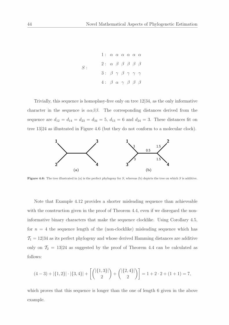
44 Novel Mathematical Aspects of Phylogenetic Estimation
S :
1 : α α α α α α
2 : α β β β β β
3 : β γ β γ γ γ
4 : β α γ β β β
Trivially, this sequence is homoplasy-free only on tree 12|34, as the only informative
character in the sequence is ααββ. The corresponding distances derived from the
sequence are d12 = d14 = d23 = d34 = 5, d13 = 6 and d24 = 3. These distances fit on
tree 13|24 as illustrated in Figure 4.6 (but they do not conform to a molecular clock).
1
42
3
(a)
4
3
3 1.5
0.5
1.5
3
1 2
(b)
Figure 4.6: The tree illustrated in (a) is the perfect phylogeny for S, whereas (b) depicts the tree on which S is additive.
Note that Example 4.12 provides a shorter misleading sequence than achieveable
with the construction given in the proof of Theorem 4.4, even if we disregard the non-
informative binary characters that make the sequence clocklike. Using Corollary 4.5,
for n = 4 the sequence length of the (non-clocklike) misleading sequence which has
T1 = 12|34 as its perfect phylogeny and whose derived Hamming distances are additive
only on T2 = 13|24 as suggested by the proof of Theorem 4.4 can be calculated as
follows:
(4 − 3) + |{1, 2}| · |{3, 4}| +[(|{1, 3}|
2
)
+
(|{2, 4}|2
)]
= 1 + 2 · 2 + (1 + 1) = 7,
which proves that this sequence is longer than the one of length 6 given in the above
example.
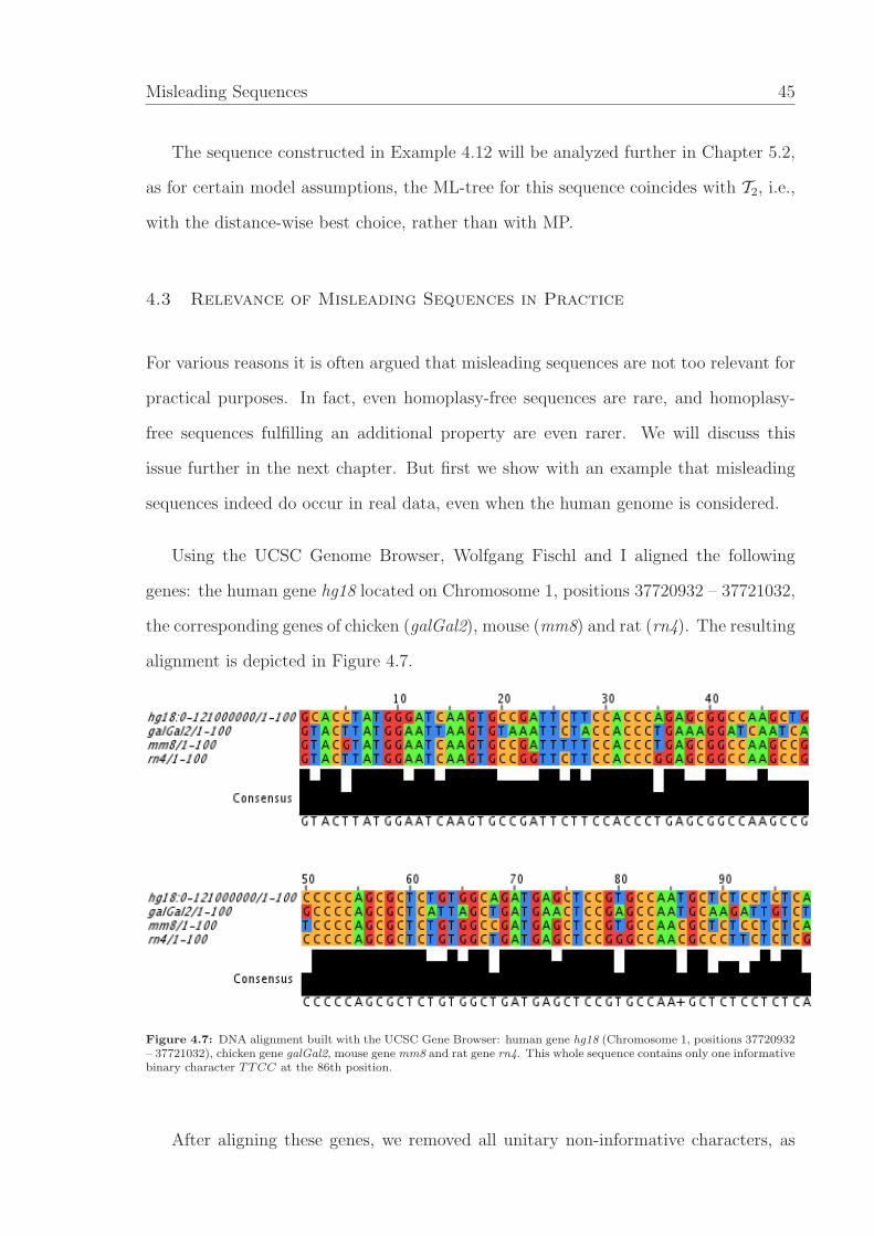
Misleading Sequences 45
The sequence constructed in Example 4.12 will be analyzed further in Chapter 5.2,
as for certain model assumptions, the ML-tree for this sequence coincides with T2, i.e.,
with the distance-wise best choice, rather than with MP.
4.3 Relevance of Misleading Sequences in Practice
For various reasons it is often argued that misleading sequences are not too relevant for
practical purposes. In fact, even homoplasy-free sequences are rare, and homoplasy-
free sequences fulfilling an additional property are even rarer. We will discuss this
issue further in the next chapter. But first we show with an example that misleading
sequences indeed do occur in real data, even when the human genome is considered.
Using the UCSC Genome Browser, Wolfgang Fischl and I aligned the following
genes: the human gene hg18 located on Chromosome 1, positions 37720932 – 37721032,
the corresponding genes of chicken (galGal2), mouse (mm8) and rat (rn4). The resulting
alignment is depicted in Figure 4.7.
Figure 4.7: DNA alignment built with the UCSC Gene Browser: human gene hg18 (Chromosome 1, positions 37720932– 37721032), chicken gene galGal2, mouse gene mm8 and rat gene rn4. This whole sequence contains only one informativebinary character TTCC at the 86th position.
After aligning these genes, we removed all unitary non-informative characters, as
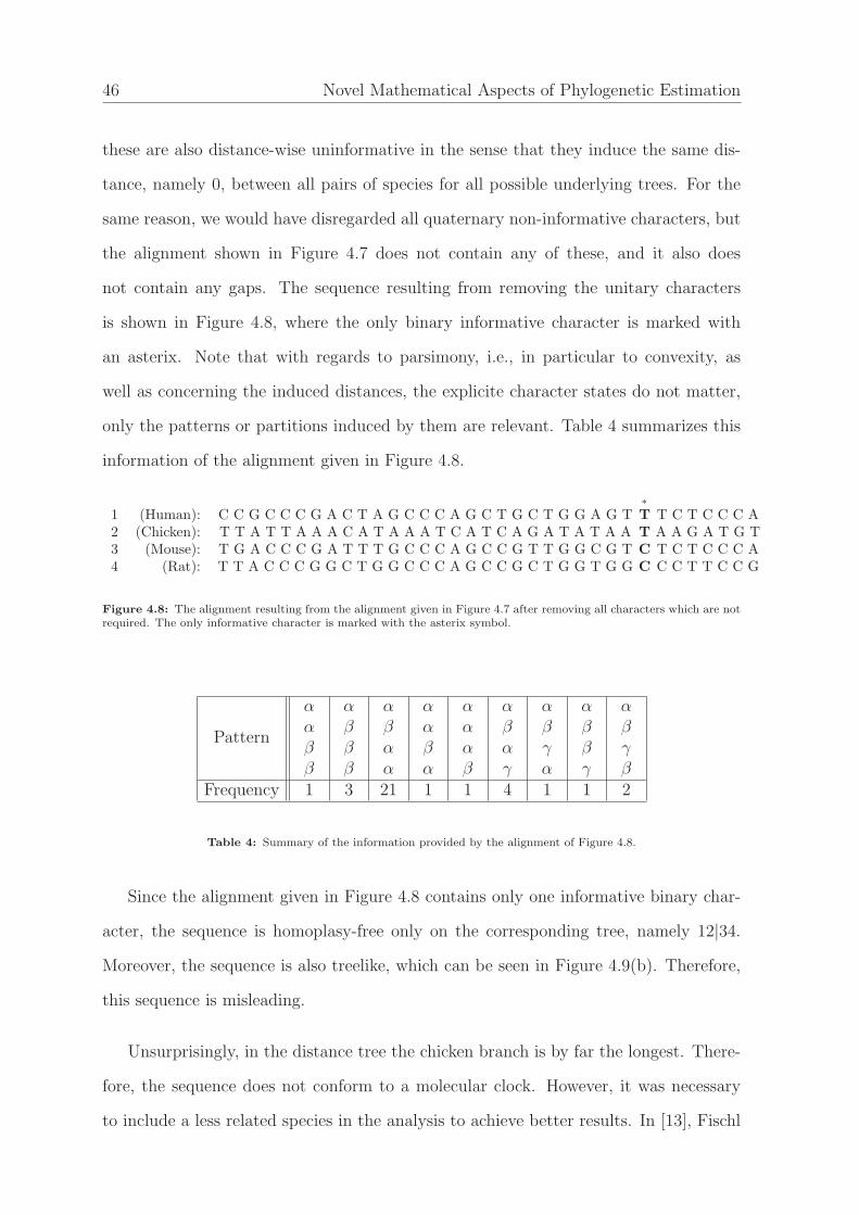
46 Novel Mathematical Aspects of Phylogenetic Estimation
these are also distance-wise uninformative in the sense that they induce the same dis-
tance, namely 0, between all pairs of species for all possible underlying trees. For the
same reason, we would have disregarded all quaternary non-informative characters, but
the alignment shown in Figure 4.7 does not contain any of these, and it also does
not contain any gaps. The sequence resulting from removing the unitary characters
is shown in Figure 4.8, where the only binary informative character is marked with
an asterix. Note that with regards to parsimony, i.e., in particular to convexity, as
well as concerning the induced distances, the explicite character states do not matter,
only the patterns or partitions induced by them are relevant. Table 4 summarizes this
information of the alignment given in Figure 4.8.
∗
1 (Human): C C G C C C G A C T A G C C C A G C T G C T G G A G T T T C T C C C A2 (Chicken): T T A T T A A A C A T A A A T C A T C A G A T A T A A T A A G A T G T3 (Mouse): T G A C C C G A T T T G C C C A G C C G T T G G C G T C T C T C C C A4 (Rat): T T A C C C G G C T G G C C C A G C C G C T G G T G G C C C T T C C G
Figure 4.8: The alignment resulting from the alignment given in Figure 4.7 after removing all characters which are notrequired. The only informative character is marked with the asterix symbol.
Pattern
ααββ
αβββ
αβαα
ααβα
αααβ
αβαγ
αβγα
αββγ
αβγβ
Frequency 1 3 21 1 1 4 1 1 2
Table 4: Summary of the information provided by the alignment of Figure 4.8.
Since the alignment given in Figure 4.8 contains only one informative binary char-
acter, the sequence is homoplasy-free only on the corresponding tree, namely 12|34.
Moreover, the sequence is also treelike, which can be seen in Figure 4.9(b). Therefore,
this sequence is misleading.
Unsurprisingly, in the distance tree the chicken branch is by far the longest. There-
fore, the sequence does not conform to a molecular clock. However, it was necessary
to include a less related species in the analysis to achieve better results. In [13], Fischl
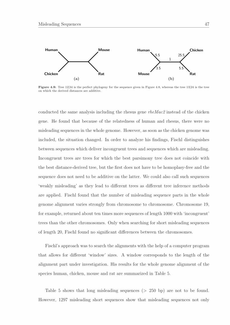
Misleading Sequences 47
Mouse
Rat
Human
Chicken
(a)
25.5
Rat
Human Chicken
Mouse
5.5
5.5
1
3.5
(b)
Figure 4.9: Tree 12|34 is the perfect phylogeny for the sequence given in Figure 4.8, whereas the tree 13|24 is the treeon which the derived distances are additive.
conducted the same analysis including the rhesus gene rheMac2 instead of the chicken
gene. He found that because of the relatedness of human and rhesus, there were no
misleading sequences in the whole genome. However, as soon as the chicken genome was
included, the situation changed. In order to analyze his findings, Fischl distinguishes
between sequences which deliver incongruent trees and sequences which are misleading.
Incongruent trees are trees for which the best parsimony tree does not coincide with
the best distance-derived tree, but the first does not have to be homoplasy-free and the
sequence does not need to be additive on the latter. We could also call such sequences
‘weakly misleading’ as they lead to different trees as different tree inference methods
are applied. Fischl found that the number of misleading sequence parts in the whole
genome alignment varies strongly from chromosome to chromosome. Chromosome 19,
for example, returned about ten times more sequences of length 1000 with ‘incongruent’
trees than the other chromosomes. Only when searching for short misleading sequences
of length 20, Fischl found no significant differences between the chromosomes.
Fischl’s approach was to search the alignments with the help of a computer program
that allows for different ‘window’ sizes. A window corresponds to the length of the
alignment part under investigation. His results for the whole genome alignment of the
species human, chicken, mouse and rat are summarized in Table 5.
Table 5 shows that long misleading sequences (> 250 bp) are not to be found.
However, 1297 misleading short sequences show that misleading sequences not only
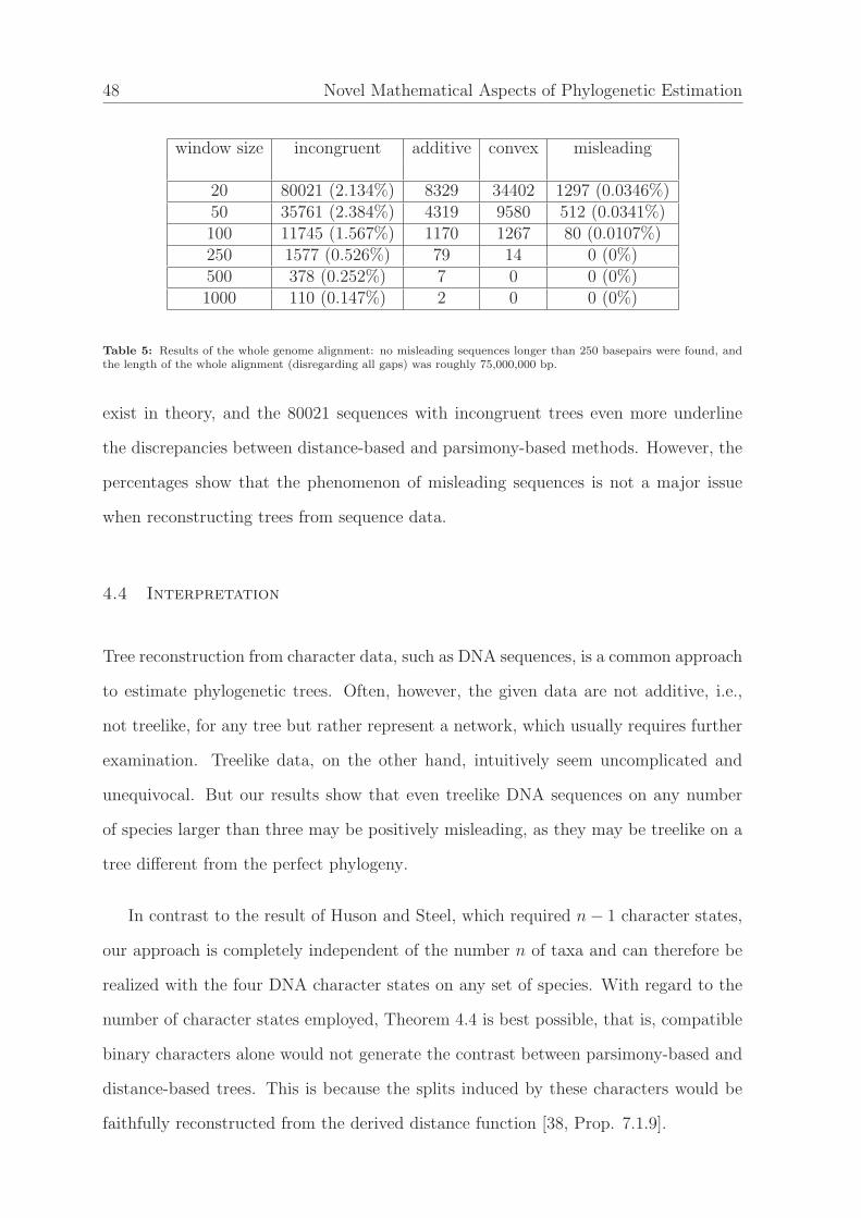
48 Novel Mathematical Aspects of Phylogenetic Estimation
window size incongruent additive convex misleading
20 80021 (2.134%) 8329 34402 1297 (0.0346%)50 35761 (2.384%) 4319 9580 512 (0.0341%)100 11745 (1.567%) 1170 1267 80 (0.0107%)250 1577 (0.526%) 79 14 0 (0%)500 378 (0.252%) 7 0 0 (0%)1000 110 (0.147%) 2 0 0 (0%)
Table 5: Results of the whole genome alignment: no misleading sequences longer than 250 basepairs were found, andthe length of the whole alignment (disregarding all gaps) was roughly 75,000,000 bp.
exist in theory, and the 80021 sequences with incongruent trees even more underline
the discrepancies between distance-based and parsimony-based methods. However, the
percentages show that the phenomenon of misleading sequences is not a major issue
when reconstructing trees from sequence data.
4.4 Interpretation
Tree reconstruction from character data, such as DNA sequences, is a common approach
to estimate phylogenetic trees. Often, however, the given data are not additive, i.e.,
not treelike, for any tree but rather represent a network, which usually requires further
examination. Treelike data, on the other hand, intuitively seem uncomplicated and
unequivocal. But our results show that even treelike DNA sequences on any number
of species larger than three may be positively misleading, as they may be treelike on a
tree different from the perfect phylogeny.
In contrast to the result of Huson and Steel, which required n − 1 character states,
our approach is completely independent of the number n of taxa and can therefore be
realized with the four DNA character states on any set of species. With regard to the
number of character states employed, Theorem 4.4 is best possible, that is, compatible
binary characters alone would not generate the contrast between parsimony-based and
distance-based trees. This is because the splits induced by these characters would be
faithfully reconstructed from the derived distance function [38, Prop. 7.1.9].
Misleading Sequences 49
Note that correcting for so-called ‘hidden changes’ under some model of sequence
evolution would not eliminate the problem. This is due to the fact that for clocklike
data, the corrections will not change the relative size of distances and the corrected
sequence would still be treelike and conform to a molecular clock on the tree which is
not the perfect phylogeny (for more details, see [38], Proposition 7.5.2).
Although ternary characters come up naturally with DNA data, Theorem 4.4 is
of rather theoretical nature because such an amount of ternary characters necessary
for split switching is out of reach with natural data (particularly when n is large).
Especially in mitochondrial DNA data sets, ternary characters are sparse. Nonetheless,
the presence of ternary characters with their different contributions to parsimony scores
and distance values can yield a minor effect that would come on top of other noise
patterns, which could adversely influence the reconstruction of distance trees and their
interpretation as phylogenetic trees. Moreover, for small n, e.g. n = 4, we have shown
in Chapter 4.3 that misleading sequences can be found in DNA data, so they do not
only exist in theory. However, the misleading sequences found were relatively small and
would therefore nowadays not be used for tree inference.
The purpose of Theorem 4.4 is not to state the importance of misleading sequences
for tree reconstruction, but rather to show that even in the perfect – and unlikely – case
of a homoplasy-free sequence whose derived distances are additive, the corresponding
trees can differ. If such a scenario is possible even if the sequence is ‘best possible’
according to both the convexity as well as the additivity criterion, it is intuitively clear
that tree reconstruction from DNA data that does incluce some homoplasies or corre-
sponds to a network rather than a tree has to be conducted even more carefully. As
Fischl has shown [13], the number of sequences giving rise to contradictory (‘incongru-
ent’) trees is, as could be expected, far higher than that of misleading sequences.
In Section 4.2, we introduced an approach which allows for sequences on four taxa
to be checked for misleadingness by just considering some equations and inequalities,
50 Novel Mathematical Aspects of Phylogenetic Estimation
but without the necessity of inferring the corresponding trees. We believe that this
approach can easily be expanded to five or more taxa, but the number of equations
and inequalities to consider will increase correspondingly. We conjecture that our char-
acterization can be used to explicitly calculate the probability of the occurrence of
misleading sequences for a given model of nucleotide substitution, which would help
answer the question of how relevant misleading sequences really are. Moreover, the se-
quence constructed in Example 4.12 also has some interesting properties concerning the
relationship of MP and ML, which will be highlighted in Chapter 5.2. In fact, the idea
used in this chapter (namely constructing a disagreement between MP and distance
methods by using the binary characters induced by the splits of the tree supposed to be
the perfect phylogeny and then adding only parsimoniously uninformative characters)
can also be used to construct a disagreement between MP and ML under certain model
assumptions. This is due to the fact that ML, just like distance methods but opposed
to MP, does not ignore parsimoniously uninformative characters.
Chapter 5
Equivalence of
Maximum Parsimony and
Maximum Likelihood
You can’t be suspicious of a tree (or accuse a bird or a squirrel of
subversion or challenge the ideology of a violet).
Hal Borland
In the previous chapter, the differences of Maximum Parsimony and distance-based tree
reconstruction methods were analyzed. In the present chapter, MP will be compared to
Maximum Likelihood (ML), which is another frequently used tree inference method. As
explained in Chapter 2, a basic difference between these two methods is that MP, unlike
ML, is not based on a specific nucleotide substitution model, and thus the methods
may perform differently under different models: if the sequences under consideration
are related by a specific model of substitution, the results of MP and ML coincide [17],
but there are also examples, such as the famous ‘Felsenstein Zone’, for which this is not
the case [10].
In 1997, Tuffley and Steel carried the analysis of MP and ML an important step
further [44]: they showed that the Nr-model with ‘no common mechanism’ is sufficient
for MP and ML to be equivalent when applied to a sequence of characters. Here, we
will present a very elementary and short proof of the Tuffley-Steel result in order to
make it more widely accessible. Along the way, we exploit some useful properties of the
likelihood function, such as its multilinearity.
Moreover, the main purpose of this chapter is to analyze this equivalence of MP and
ML further by considering slightly modified model assumptions that are of biological
relevance. For instance, MP is often assumed to be justified whenever the nucleotide
51
52 Novel Mathematical Aspects of Phylogenetic Estimation
substitution probabilities are small (see, e.g., [12], p. 101). Therefore, we restrict the
model by placing an upper bound on these probabilities, and find that under no common
mechanism, MP and ML are no longer equivalent. Moreover, the equivalence of MP and
ML under a ‘no common mechanism model’ also fails under the constraint of a mole-
cular clock, even without a bound on the substitution probabilities. These two claims
will be established by constructing counterexamples that are minimal with respect to
the number of taxa. To construct our examples, we exploit a useful property of the
likelihood function for a ‘no common mechanism’ model, namely that it is multilinear
in the substitution probabilities. This fact underlies Equation 18 and Lemma 2 in [44],
which we use in our arguments. We will show that some ideas which are useful to
construct a disagreement of MP and ML are related to the ideas used in Chapter 4.
Additionally, we prove bounds on the ML-value of a given sequence of characters on
a tree, and use them to show that it is possible to choose sufficiently small substitution
probabilities (depending on the number of taxa, the number of characters and the
number of states) so that every tree chosen by ML is also a most parsimonious tree.
5.1 Elementary Proof of the Tuffley-Steel Result
We begin with explicitly stating the equivalence of MP and ML in the following theorem.
We first prove it for a single character, and then generalize the proof to a sequence of
characters, assuming no common mechanism.
Theorem 5.1. (Tuffley and Steel 1997) Let m ∈ N and S := f1 . . . fm be a sequence
of r-state characters on a phylogenetic X-tree T . Then, under the Nr-model with no
common mechanism, the maximum likelihood of S and its parsimony score are related
by
max P (S|T ) = r−lT (S)−m, (27)
which implies that Maximum Likelihood and Maximum Parsimony both choose the same
tree(s).
Equivalence of Maximum Parsimony and Maximum Likelihood 53
We first consider the case m = 1, i.e., a single character f . Thus, we first show
max P (f) = r−lT (f)−1. (28)
Note that in the Nr-model, P (f) = 1r· P (f |f(1) = c1), where c1 is the character
state assigned to leaf taxon 1 (for details on the so-called reversibility of the Nr-model,
which is the reason why the actual root position does not matter, the reader is referred
to [11]). Thus, in order to show (28) it is sufficient to show
max P (f |f(1) = c1) = r−lT (f). (29)
We prove (29) by first showing with Lemma 5.2 that r−lT (f) is a lower bound for
max P (f |f(1) = c1). Then, Lemma 5.5 completes the proof by demonstrating that
r−lT (f) is additionally an upper bound for P (f |f(1) = c1).
Lemma 5.2.
max P (f |f(1) = c1) ≥ r−lT (f)
Proof. Consider a most parsimonious extension g of f . Then, g requires exactly
lT (f) substitutions. We assign substitution probability 1r
to those edges on which
a substitution occurs in g, and substitution probability 0 to all other edges. Then,
P (g|f(1) = c1) = r−lT (f). The lower bound for max P (f |f(1) = c1) now follows from
the fact that P (f |f(1) = c1) =∑
g
P (g|f(1) = c1).
Lemma 5.2 states that r−lT (f) is a lower bound for maxP (f |f(1) = c1). In order
to show that it is also an upper bound, we need some preliminaries concerning the
likelihood function. These will be provided by Lemma 5.3 and Corollary 5.4.
54 Novel Mathematical Aspects of Phylogenetic Estimation
Lemma 5.3. Let h be a function from the k-dimensional box Bk = [0, t]k to the real
numbers, i.e., h : Bk → R. If h is multilinear, then there is a corner p of Bk such that
h(p) ≥ h(x) for every point x in Bk.
Proof. We use an arbitrary point x := (x1, x2, . . . , xk) in Bk as the initial value of a
greedy hill climbing algorithm. Suppose we fix the values xj for all j other than i. Since
h is multilinear, h(x) then takes the form axi + b. Now we distinguish between two
cases:
1. a ≥ 0. In this case, we replace xi by t.
2. a < 0. In this case, we replace xi by 0.
In either case, the value of h(x) cannot decrease. Repeating this step for all i = 1, . . . , k,
one eventually arrives at a corner p of the box Bk, where h(p) ≥ h(x). The particular
corner p obtained by the above procedure depends on the initial choice of x. Thus, as a
last step we select a corner of Bk that maximizes h among all corners. This completes
the proof.
We are now in the position to make first statements on the likelihood function.
Corollary 5.4. Let f be a character on a phylogenetic X-tree T . Then under the Nr-
model with all substitution probabilities bounded by u, where 0 ≤ u ≤ 1r, the likelihood
P (f |T ) can be maximized at a point where all substitution probabilities are either 0 or
u.
Proof. First, recall that
P (f |f(1) = c1) =∑
g
P (g|f(1) = c1), (30)
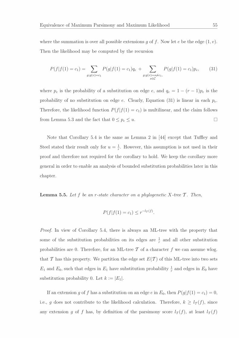
Equivalence of Maximum Parsimony and Maximum Likelihood 55
where the summation is over all possible extensions g of f . Now let e be the edge (1, v).
Then the likelihood may be computed by the recursion
P (f |f(1) = c1) =∑
g:g(v)=c1
P (g|f(1) = c1)qe +∑
g:g(v)=s 6=c1,s∈C
P (g|f(1) = c1)pe, (31)
where pe is the probability of a substitution on edge e, and qe = 1 − (r − 1)pe is the
probability of no substitution on edge e. Clearly, Equation (31) is linear in each pe.
Therefore, the likelihood function P (f |f(1) = c1) is multilinear, and the claim follows
from Lemma 5.3 and the fact that 0 ≤ pe ≤ u.
Note that Corollary 5.4 is the same as Lemma 2 in [44] except that Tuffley and
Steel stated their result only for u = 1r. However, this assumption is not used in their
proof and therefore not required for the corollary to hold. We keep the corollary more
general in order to enable an analysis of bounded substitution probabilities later in this
chapter.
Lemma 5.5. Let f be an r-state character on a phylogenetic X-tree T . Then,
P (f |f(1) = c1) ≤ r−lT (f).
Proof. In view of Corollary 5.4, there is always an ML-tree with the property that
some of the substitution probabilities on its edges are 1r
and all other substitution
probabilities are 0. Therefore, for an ML-tree T of a character f we can assume wlog.
that T has this property. We partition the edge set E(T ) of this ML-tree into two sets
E1 and E0, such that edges in E1 have substitution probability 1r
and edges in E0 have
substitution probability 0. Let k := |E1|.
If an extension g of f has a substitution on an edge e in E0, then P (g|f(1) = c1) = 0,
i.e., g does not contribute to the likelihood calculation. Therefore, k ≥ lT (f), since
any extension g of f has, by definition of the parsimony score lT (f), at least lT (f)
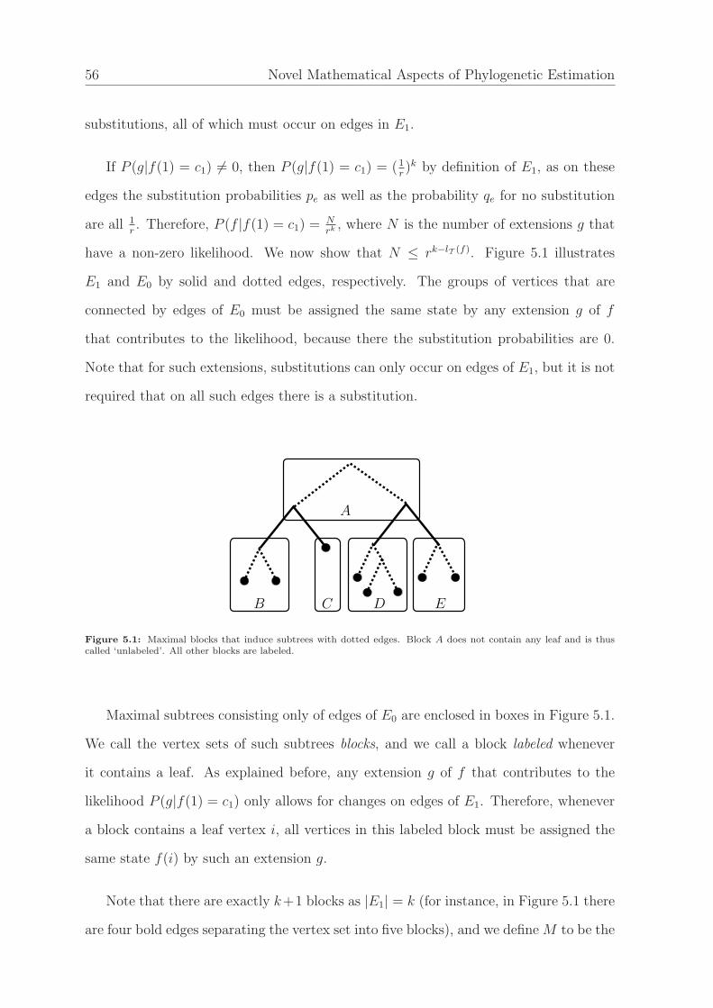
56 Novel Mathematical Aspects of Phylogenetic Estimation
substitutions, all of which must occur on edges in E1.
If P (g|f(1) = c1) 6= 0, then P (g|f(1) = c1) = (1r)k by definition of E1, as on these
edges the substitution probabilities pe as well as the probability qe for no substitution
are all 1r. Therefore, P (f |f(1) = c1) = N
rk , where N is the number of extensions g that
have a non-zero likelihood. We now show that N ≤ rk−lT (f). Figure 5.1 illustrates
E1 and E0 by solid and dotted edges, respectively. The groups of vertices that are
connected by edges of E0 must be assigned the same state by any extension g of f
that contributes to the likelihood, because there the substitution probabilities are 0.
Note that for such extensions, substitutions can only occur on edges of E1, but it is not
required that on all such edges there is a substitution.
E
A
CB D
Figure 5.1: Maximal blocks that induce subtrees with dotted edges. Block A does not contain any leaf and is thuscalled ‘unlabeled’. All other blocks are labeled.
Maximal subtrees consisting only of edges of E0 are enclosed in boxes in Figure 5.1.
We call the vertex sets of such subtrees blocks, and we call a block labeled whenever
it contains a leaf. As explained before, any extension g of f that contributes to the
likelihood P (g|f(1) = c1) only allows for changes on edges of E1. Therefore, whenever
a block contains a leaf vertex i, all vertices in this labeled block must be assigned the
same state f(i) by such an extension g.
Note that there are exactly k+1 blocks as |E1| = k (for instance, in Figure 5.1 there
are four bold edges separating the vertex set into five blocks), and we define M to be the
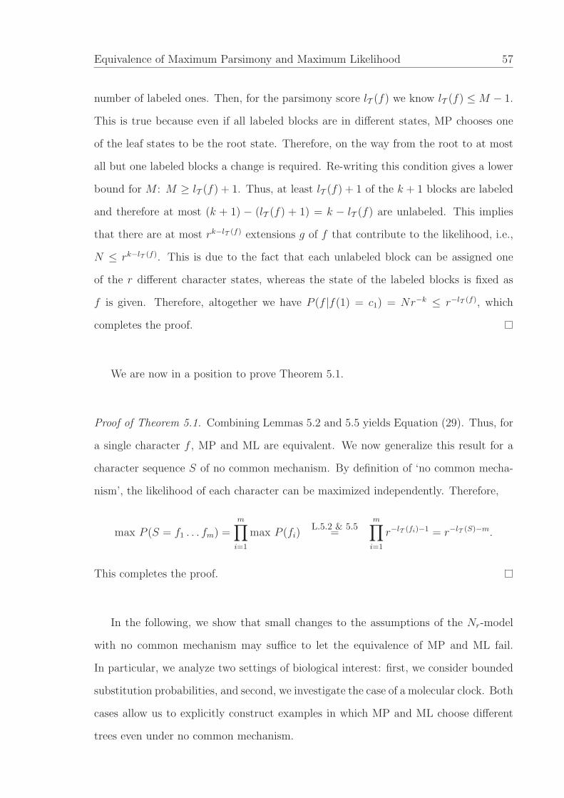
Equivalence of Maximum Parsimony and Maximum Likelihood 57
number of labeled ones. Then, for the parsimony score lT (f) we know lT (f) ≤ M − 1.
This is true because even if all labeled blocks are in different states, MP chooses one
of the leaf states to be the root state. Therefore, on the way from the root to at most
all but one labeled blocks a change is required. Re-writing this condition gives a lower
bound for M : M ≥ lT (f) + 1. Thus, at least lT (f) + 1 of the k + 1 blocks are labeled
and therefore at most (k + 1) − (lT (f) + 1) = k − lT (f) are unlabeled. This implies
that there are at most rk−lT (f) extensions g of f that contribute to the likelihood, i.e.,
N ≤ rk−lT (f). This is due to the fact that each unlabeled block can be assigned one
of the r different character states, whereas the state of the labeled blocks is fixed as
f is given. Therefore, altogether we have P (f |f(1) = c1) = Nr−k ≤ r−lT (f), which
completes the proof.
We are now in a position to prove Theorem 5.1.
Proof of Theorem 5.1. Combining Lemmas 5.2 and 5.5 yields Equation (29). Thus, for
a single character f , MP and ML are equivalent. We now generalize this result for a
character sequence S of no common mechanism. By definition of ‘no common mecha-
nism’, the likelihood of each character can be maximized independently. Therefore,
max P (S = f1 . . . fm) =m∏
i=1
max P (fi)L.5.2 & 5.5
=m∏
i=1
r−lT (fi)−1 = r−lT (S)−m.
This completes the proof.
In the following, we show that small changes to the assumptions of the Nr-model
with no common mechanism may suffice to let the equivalence of MP and ML fail.
In particular, we analyze two settings of biological interest: first, we consider bounded
substitution probabilities, and second, we investigate the case of a molecular clock. Both
cases allow us to explicitly construct examples in which MP and ML choose different
trees even under no common mechanism.
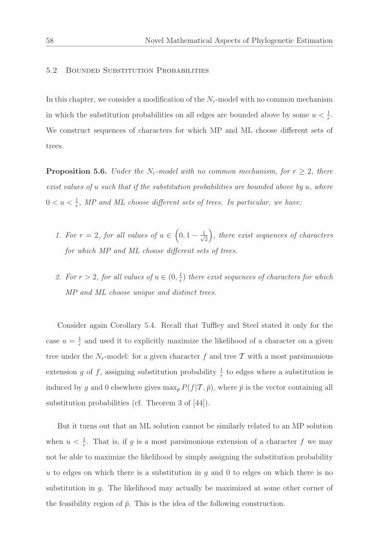
58 Novel Mathematical Aspects of Phylogenetic Estimation
5.2 Bounded Substitution Probabilities
In this chapter, we consider a modification of the Nr-model with no common mechanism
in which the substitution probabilities on all edges are bounded above by some u < 1r.
We construct sequences of characters for which MP and ML choose different sets of
trees.
Proposition 5.6. Under the Nr-model with no common mechanism, for r ≥ 2, there
exist values of u such that if the substitution probabilities are bounded above by u, where
0 < u < 1r, MP and ML choose different sets of trees. In particular, we have:
1. For r = 2, for all values of u ∈(
0, 1 − 1√2
)
, there exist sequences of characters
for which MP and ML choose different sets of trees.
2. For r > 2, for all values of u ∈ (0, 1r) there exist sequences of characters for which
MP and ML choose unique and distinct trees.
Consider again Corollary 5.4. Recall that Tuffley and Steel stated it only for the
case u = 1r
and used it to explicitly maximize the likelihood of a character on a given
tree under the Nr-model: for a given character f and tree T with a most parsimonious
extension g of f , assigning substitution probability 1r
to edges where a substitution is
induced by g and 0 elsewhere gives maxp P (f |T , p), where p is the vector containing all
substitution probabilities (cf. Theorem 3 of [44]).
But it turns out that an ML solution cannot be similarly related to an MP solution
when u < 1r. That is, if g is a most parsimonious extension of a character f we may
not be able to maximize the likelihood by simply assigning the substitution probability
u to edges on which there is a substitution in g and 0 to edges on which there is no
substitution in g. The likelihood may actually be maximized at some other corner of
the feasibility region of p. This is the idea of the following construction.
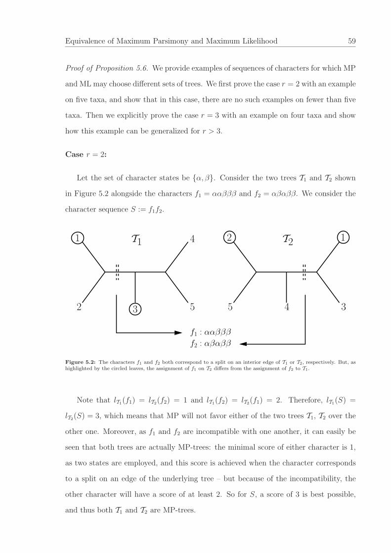
Equivalence of Maximum Parsimony and Maximum Likelihood 59
Proof of Proposition 5.6. We provide examples of sequences of characters for which MP
and ML may choose different sets of trees. We first prove the case r = 2 with an example
on five taxa, and show that in this case, there are no such examples on fewer than five
taxa. Then we explicitly prove the case r = 3 with an example on four taxa and show
how this example can be generalized for r > 3.
Case r = 2:
Let the set of character states be {α, β}. Consider the two trees T1 and T2 shown
in Figure 5.2 alongside the characters f1 = ααβββ and f2 = αβαββ. We consider the
character sequence S := f1f2.
5
f2 : αβαββ
1
3
4
52 4
T1 T21
3
2
f1 : ααβββ
Figure 5.2: The characters f1 and f2 both correspond to a split on an interior edge of T1 or T2, respectively. But, ashighlighted by the circled leaves, the assignment of f1 on T2 differs from the assignment of f2 to T1.
Note that lT1(f1) = lT2(f2) = 1 and lT1(f2) = lT2(f1) = 2. Therefore, lT1(S) =
lT2(S) = 3, which means that MP will not favor either of the two trees T1, T2 over the
other one. Moreover, as f1 and f2 are incompatible with one another, it can easily be
seen that both trees are actually MP-trees: the minimal score of either character is 1,
as two states are employed, and this score is achieved when the character corresponds
to a split on an edge of the underlying tree – but because of the incompatibility, the
other character will have a score of at least 2. So for S, a score of 3 is best possible,
and thus both T1 and T2 are MP-trees.
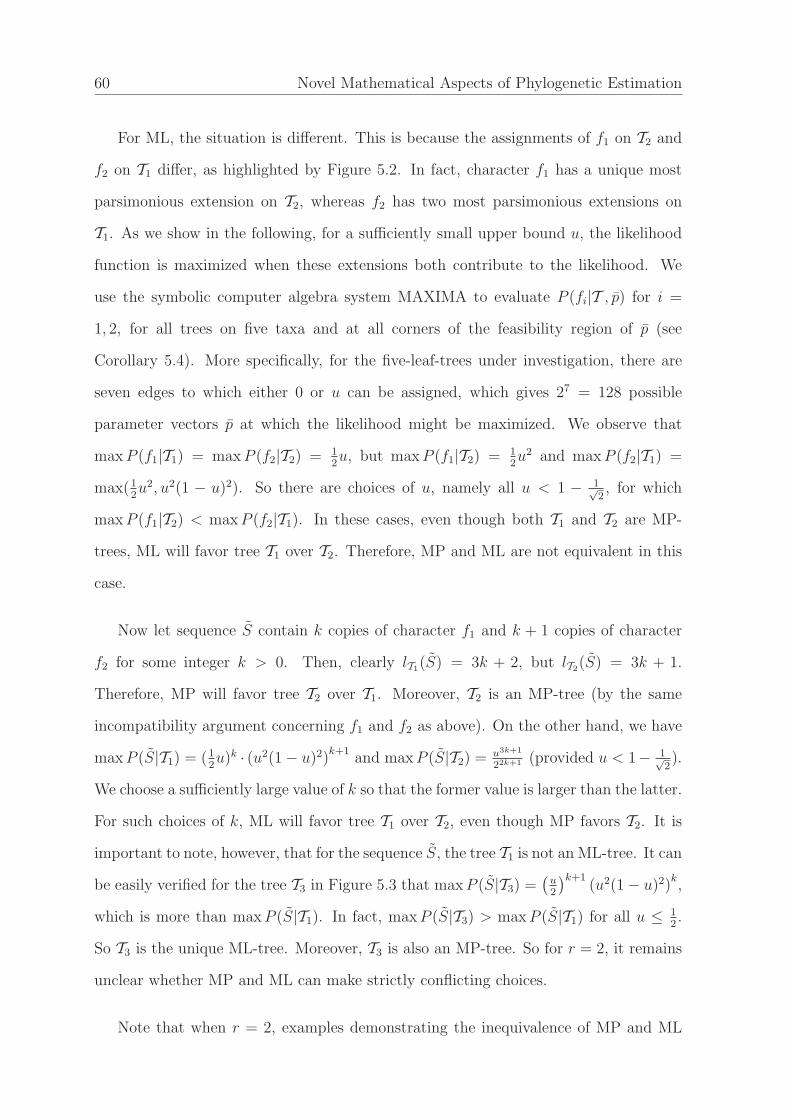
60 Novel Mathematical Aspects of Phylogenetic Estimation
For ML, the situation is different. This is because the assignments of f1 on T2 and
f2 on T1 differ, as highlighted by Figure 5.2. In fact, character f1 has a unique most
parsimonious extension on T2, whereas f2 has two most parsimonious extensions on
T1. As we show in the following, for a sufficiently small upper bound u, the likelihood
function is maximized when these extensions both contribute to the likelihood. We
use the symbolic computer algebra system MAXIMA to evaluate P (fi|T , p) for i =
1, 2, for all trees on five taxa and at all corners of the feasibility region of p (see
Corollary 5.4). More specifically, for the five-leaf-trees under investigation, there are
seven edges to which either 0 or u can be assigned, which gives 27 = 128 possible
parameter vectors p at which the likelihood might be maximized. We observe that
max P (f1|T1) = max P (f2|T2) = 12u, but max P (f1|T2) = 1
2u2 and max P (f2|T1) =
max(12u2, u2(1 − u)2). So there are choices of u, namely all u < 1 − 1√
2, for which
max P (f1|T2) < max P (f2|T1). In these cases, even though both T1 and T2 are MP-
trees, ML will favor tree T1 over T2. Therefore, MP and ML are not equivalent in this
case.
Now let sequence S contain k copies of character f1 and k + 1 copies of character
f2 for some integer k > 0. Then, clearly lT1(S) = 3k + 2, but lT2(S) = 3k + 1.
Therefore, MP will favor tree T2 over T1. Moreover, T2 is an MP-tree (by the same
incompatibility argument concerning f1 and f2 as above). On the other hand, we have
max P (S|T1) = (12u)k · (u2(1 − u)2)
k+1and max P (S|T2) = u3k+1
22k+1 (provided u < 1− 1√2).
We choose a sufficiently large value of k so that the former value is larger than the latter.
For such choices of k, ML will favor tree T1 over T2, even though MP favors T2. It is
important to note, however, that for the sequence S, the tree T1 is not an ML-tree. It can
be easily verified for the tree T3 in Figure 5.3 that maxP (S|T3) =(
u2
)k+1(u2(1 − u)2)
k,
which is more than max P (S|T1). In fact, max P (S|T3) > max P (S|T1) for all u ≤ 12.
So T3 is the unique ML-tree. Moreover, T3 is also an MP-tree. So for r = 2, it remains
unclear whether MP and ML can make strictly conflicting choices.
Note that when r = 2, examples demonstrating the inequivalence of MP and ML
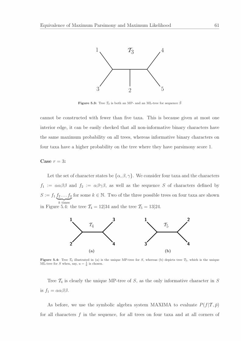
Equivalence of Maximum Parsimony and Maximum Likelihood 61
4
5
1
3 2
T3
Figure 5.3: Tree T3 is both an MP- and an ML-tree for sequence S
cannot be constructed with fewer than five taxa. This is because given at most one
interior edge, it can be easily checked that all non-informative binary characters have
the same maximum probability on all trees, whereas informative binary characters on
four taxa have a higher probability on the tree where they have parsimony score 1.
Case r = 3:
Let the set of character states be {α, β, γ}. We consider four taxa and the characters
f1 := ααββ and f2 := αβγβ, as well as the sequence S of characters defined by
S := f1 f2 . . . f2︸ ︷︷ ︸
k times
for some k ∈ N. Two of the three possible trees on four taxa are shown
in Figure 5.4: the tree T4 = 12|34 and the tree T5 = 13|24.
1
42
3
T4
(a)
1
4
T5
2
3
(b)
Figure 5.4: Tree T4 illustrated in (a) is the unique MP-tree for S, whereas (b) depicts tree T5, which is the uniqueML-tree for S when, say, u = 1
8is chosen.
Tree T4 is clearly the unique MP-tree of S, as the only informative character in S
is f1 = ααββ.
As before, we use the symbolic algebra system MAXIMA to evaluate P (f |T , p)
for all characters f in the sequence, for all trees on four taxa and at all corners of
62 Novel Mathematical Aspects of Phylogenetic Estimation
the feasibility region of p. We observed that max P (f2|T4) = u2
3and max P (f2|T5) =
u2(1 − 2u). Therefore, for all u < 1r, we have max P (f2|T5) > max P (f2|T4). Now for
any u < 1r, a sufficiently large value of k may be chosen such that max P (S|T5)
max P (S|T4)> 1. We do
not analyze the character f1, although the actual choice of k will depend on the ratio
max P (f1|T5)max P (f1|T4)
and on u. Therefore, MP and ML choose different trees in this three-state
setting. Moreover, it can be easily verified that for the third topology on four taxa,
namely T6 = 14|23, we have max P (S|T6) < max P (S|T5) for all choices of u ≤ 13. So,
T5 is the unique ML-tree, whereas T4 is the unique MP-tree in this setting. So MP and
ML make strictly conflicting choices.
Case r > 3:
Let the set of states be C := {α, β, γ, δ1, δ2, . . . , δr−3}. Let D := {δ1, δ2, . . . , δr−3}.
We analyze four taxa and the same characters f1 := ααββ and f2 := αβγβ that were
analyzed in the case r = 3, but this time under the Nr-model with r > 3. Again we
consider the sequence of characters S := f1 f2 . . . f2︸ ︷︷ ︸
k times
.
We only sketch the proof in this case. In particular, we indicate how the expressions
for the likelihood function may be written regardless of the number of states.
The expressions for P (fi|Tj) for i = 1, 2 and j = 1, 2, 3 can be written in a simple
manner since the states δi do not occur in S. For example, let the substitution prob-
abilities on the edges of a four-taxa tree T be p = (pi, i = 1, 2, . . . , 5), where pi (for
i ∈ {1, 2, 3, 4}) are the substitution probabilities on the pending edges adjacent to taxa
1, 2, 3, 4, respectively, and p5 is the substitution probability on the internal edge. Let
u and v be the internal vertices of T . We write P (fi|T , p) =∑
g P (g|T , p), where the
summation is over all extensions g of fi.
Now observe that if g and h are two extensions of a character f , then we have
P (g|T , p) = P (h|T , p) if g(u), h(u) ∈ D and g(v) = h(v) = s /∈ D (or vice versa with
the roles of u and v interchanged).
Equivalence of Maximum Parsimony and Maximum Likelihood 63
Therefore:∑
g : g(u) ∈ D,
g(v) = s /∈ D
P (g|T , p) = (r − 3)P (h|T , p),
where h is an extension of f for which h(u) = δ1 and h(v) = s.
Similarly:∑
g : g(u) = s /∈ D,
g(v) ∈ D
P (g|T , p) = (r − 3)P (h|T , p),
where h is an extension of f for which h(u) = s and h(v) = δ1.
Finally:∑
g : g(u) ∈ D,
g(v) ∈ D
P (g|T , p) = (r − 3)(1 − 3p5)p1p2p3p4,
With these observations, it is possible to write the expressions for computing P (fi|Tj)
in a computer algebra system like MAXIMA. As in the case r = 3, we analyzed only
P (f2|T4) and P (f2|T5), and verified that maxP (f2|T5) ≥ u2(3−2ru)r
and max P (f2|T4) =
u2
r. Since (3−2ru) > 1 for all u < 1
r, there is a k for which max P (S|T5) > max P (S|T4).
This means that ML will favor T5 over T4, even though T4 is the unique MP-tree in this
setting.
Remark 1. It is important to state that in the examples for r ≥ 3 introduced in the
proof of Proposition 5.6, where the number of taxa is bounded (in fact, it is only 4), as
u approaches 1r, we require the sequence length k +1, and thus k, to tend to infinity for
ML and MP to make different choices. However, this is a necessary property of any such
example for which the number of taxa is bounded: For any fixed character sequence
S, the continuity of the likelihood function and the Tuffley-Steel result (Theorem 5.1)
imply that there is a positive real number ǫ(S) such that if u > 1r− ǫ(S), then ML and
MP choose the same sets of trees. Therefore, for a bounded number of taxa, since there
are only finitely many sequences of length at most k +1, we set ǫ := minS(ǫ(S)), where
64 Novel Mathematical Aspects of Phylogenetic Estimation
the minimization takes place over all character sequences of length at most k + 1, and
conclude that MP and ML would be equivalent (in the sense of the Tuffley-Steel result)
for all u > 1r−ǫ, for all sequences of length at most k+1. Therefore, as u approaches 1
r,
the sequence length k + 1 of sequences for which MP and ML make conflicting choices
has to tend to infinity.
Note that the role of the N2-model with no common mechanism in Proposition 5.6
is different than that of the Nr-model with no common mechanism for r > 2: for r = 2,
we only state that the sets of trees chosen by MP and ML may be different for certain
choices of values for the upper bound u. In particular, our proof shows that some
MP-trees may not be ML-trees in this setting, but it is still unknown if the opposite
can also happen. The intuitive reason why the binary case might indeed be different is
due to the relationship of sequence S = f1f2 . . . f2 as used in Propositon 5.6 and the
(distance-wise) misleading sequences as introduced in Chapter 4. In fact, S = f1f2f2f2
(i.e. the particular case with three copies of character f2) is a shorter version of the
sequence constructed in Chapter 4.2; only two characters are missing, namely αβγα
and αββγ – and trivially, the ML-values of these characters on T4 and T5 (depicted in
Figure 5.4) are equal (as the pattern of both characters is equal on both trees). It can
be easily verified that the ML-value of each of these characters on both trees is u2
3. So
adding these characters to the sequence used in Proposition 5.6 does not change the
example: in fact, this sequence, which was constructed in Chapter 4.2 as a case in which
the perfect phylogeny and the tree induced by the derived distances differ, is also an
example for a sequence where a certain choice of an upper bound u will make MP and
ML differ (but note that the shorter version of this sequence, which for certain values
of u causes a disagreement of MP and ML, is not a misleading sequence concerning
the Hamming distance as it is not even treelike). In fact, for these choices of u, e.g.
u = 18
as shown in the proof of Proposition 5.6, ML will agree with the tree on which
the Hamming distances are treelike, namely T2, whereas MP will naturally favor T1 as
the only informative character in the sequence is f1 = ααββ.
Equivalence of Maximum Parsimony and Maximum Likelihood 65
We now complement the above inequivalence results by showing that for sufficiently
small choices of u, all ML-trees are also MP-trees. To prove this result, we first establish
lower and upper bounds for the maximum probability of observing a character given a
tree.
Proposition 5.7. Let T be a phylogenetic X-tree, where |X| = n. Let f be a character
on X. Then under the Nr-model with no common mechanism and with all substitution
probabilities bounded by u, where 0 ≤ u < 1r, we have
(1
r
)
ulT (f) ≤ max P (f |T ) ≤ rm−3ulT (f),
where max P (f |T ) is the maximum likelihood of f on T and lT (f) is the parsimony
score of f on T .
Proof. For the lower bound, just as in the Tuffley-Steel approach explained above, we
take a most parsimonious extension g of f and assign substitution probability u to each
edge that has a substitution in g and 0 to all other edges. Considering the r possible root
states (for an arbitrarily chosen root), this gives the lower bound for maxp P (f |T , p).
To prove the upper bound, we observe that there are exactly rn−2 extensions of f ,
where n−2 is the number of internal vertices, each of which may be assigned any of the
r states. We will now analyze these extensions. Let g be any extension of f . For any
assignment of substitution probabilities to the edges of the tree, the value of P (g|T , p)
for an assignment of probabilities that maximizes P (f |T , p) is either 0 (if one of the
edges on which there is a substitution in g has been assigned a substitution probability
0) or is given by
maxp
P (g|T , p) =1
ruk1(1 − (r − 1)u)k2 ≤ 1
ruk1 ≤ 1
rulT (f), (32)
where k1 ≥ lT (f) is the number of edges on which there is a substitution in g and
k2 is the number of edges which require no substitution in g but have been assigned
66 Novel Mathematical Aspects of Phylogenetic Estimation
substitution probability u. The factor 1r
is due to the r possible choices for the root
state.
By Equation (32), each extension of f has a likelihood of at most 1rulT (f). The upper
bound now follows by summing the likelihoods of all extensions.
Now we will use the bounds for the maximum likelihood to derive the desired con-
clusion on ML-trees.
Theorem 5.8. Let S = f1f2 . . . fm be a character sequence and let Ta and Tb be two
phylogenetic X-trees, where |X| = n. Then under the Nr-model with no common mech-
anism and with all substitution probabilities bounded by u, where 0 ≤ u < 1r, we have
for sufficiently small choices of u
lTb(S) < lTa(S) ⇒ max P (S|Tb) > max P (S|Ta),
i.e., if Tb is parsimoniously better than Ta, it also has a better ML-value.
Proof. By Proposition 5.7 we have
max P (S|Ta) ≤ r(n−3)mu∑
i lTa (fi) (33)
and
max P (S|Tb) ≥(
1
r
)m
u∑
i lTb(fi). (34)
Note that for any positive integers a and b such that b < a and any positive constant
c, for sufficiently small values of u we have ua < cub. Now by assumption we have
b :=∑
i lTb(fi) <
∑
i lTa(fi) =: a. With c := min(1, (rn+(n−3)n)−1), using this argument
for Equations (33) and (34), we get for sufficiently small values of u that max P (S|Tb) >
max P (S|Ta).
Equivalence of Maximum Parsimony and Maximum Likelihood 67
Corollary 5.9. Let S be sequence of m characters on a set of n taxa. Then there is
an ǫ = ǫ(n,m, r) such that under the Nr-model with no common mechanism and with
all substitution probabilities subject to an upper bound u ∈ [0, ǫ), all ML-trees of S are
also MP-trees.
Proof. Let ǫ be ‘sufficiently small’ with respect to Theorem 5.8, and let Tb be any MP-
tree for S. Let Ta be another tree that is not a most parsimonious tree. That is, lTb(S) <
lTa(S). Therefore, by Theorem 5.8, for u ∈ [0, ǫ), we have max P (S|Tb) > max P (S|Ta).
Thus, Ta cannot be an ML-tree, implying that all ML-trees are also MP-trees.
5.3 Molecular Clock
We now prove a statement similar to Proposition 5.6, but instead of considering bounded
substitution probabilities, we analyze substitution probabilities which conform to a
molecular clock. Moreover, we consider only the three-state symmetric model. Under
the N3-model, we consider two cases (for any phylogenetic X-tree rooted at some root ρ
and conforming to a molecular clock). In the first case, the probability of a substitution
from the root to any of its leaves is bounded above by pmax ∈ [0, 13). In the second case,
the probability of a substitution from the root to any of its leaves is bounded above by
pmax = 13
(as suggested by the N3-model).
Proposition 5.10. Under the N3-model with no common mechanism, with the substi-
tution probabilities constrained by a molecular clock, MP and ML are not equivalent for
any bound pmax ∈ [0, 13].
Proof. We show the inequivalence first for pmax ∈ [0, 13), and then for pmax = 1
3.
Consider the two rooted trees T1 and T2 along with substitution probabilities pi and
pi, respectively, on their edges as shown in Figure 5.5. The trees have the same shape
but different leaf labels, and possibly different probabilities of a substitution from the
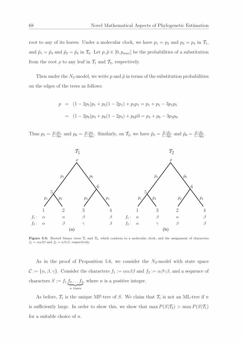
68 Novel Mathematical Aspects of Phylogenetic Estimation
root to any of its leaves. Under a molecular clock, we have p1 = p2 and p3 = p4 in T1,
and p1 = p3 and p2 = p4 in T2. Let p, p ∈ [0, pmax] be the probabilities of a substitution
from the root ρ to any leaf in T1 and T2, respectively.
Then under the N3-model, we write p and p in terms of the substitution probabilities
on the edges of the trees as follows:
p = (1 − 2p5)p1 + p5(1 − 2p1) + p5p1 = p1 + p5 − 3p1p5
= (1 − 2p6)p3 + p6(1 − 2p3) + p6p3 = p3 + p6 − 3p3p6.
Thus p5 = p−p1
1−3p1and p6 = p−p3
1−3p3. Similarly, on T2, we have p5 = p−p1
1−3p1and p6 = p−p2
1−3p2.
5
3
β
β
2
αf1 :
αf2 :
1
α
β
β
4
ρ
T1
6
p2 p4
p6p5
p3p1
γ
(a)
β
β
4
ρ
T2
6
5
p5 p6
p3p1 p4p2
3 2
f1 :
αf2 :
1
α β α
γ β
(b)
Figure 5.5: Rooted binary trees T1 and T2, which conform to a molecular clock, and the assignment of charactersf1 = ααββ and f2 = αβγβ, respectively.
As in the proof of Proposition 5.6, we consider the N3-model with state space
C := {α, β, γ}. Consider the characters f1 := ααββ and f2 := αβγβ, and a sequence of
characters S := f1 f2 . . . f2︸ ︷︷ ︸
n times
, where n is a positive integer.
As before, T1 is the unique MP-tree of S. We claim that T1 is not an ML-tree if n
is sufficiently large. In order to show this, we show that maxP (S|T2) > max P (S|T1)
for a suitable choice of n.
Equivalence of Maximum Parsimony and Maximum Likelihood 69
Since we assume no common mechanism, we have
max P (S|T2)
max P (S|T1)=
(max P (f1|T2))(max P (f2|T2))n
(max P (f1|T1))(max P (f2|T1))n.
We now demonstrate, without calculating maxP (f1|T1) and max P (f1|T2) explicitly
(but using the fact that these values are positive), that maxP (f2|T2) > max P (f2|T1)
for all values of pmax. This allows us to choose a sufficiently large value of n so that the
ratio above is more than 1.
First we seek to maximize:
P (f2|T1, p) =∑
c∈CP (f2|T1, p, ρ = c)P (ρ = c) =
1
3
∑
c∈CP (f2|T1, p, ρ = c).
Using the computer algebra system MAXIMA, we expand the right-hand side of
this equation by summing the probabilities over all possible assignments of states to
the internal nodes 5 and 6, and substitute p5 = p−p1
1−3p1and p6 = p−p3
1−3p3to obtain:
P (f2|T1, p) =p1p3(3p1p3 − 2p1 − 2p3 + 1 + 2p − 3p2)
3.
Observe that for any fixed values of p1+p3 and p, the expression above is maximized
when p1p3 is maximized, i.e. when p1 = p3. Therefore, we can substitute p1 for p3 and
maximize the resulting expression given by:
p21(1 − p − p1)(1 + 3p − 3p1)
3.
Under the constraint p ∈ [0, pmax], straightforward arguments show that the expres-
sion shown above has a maximum at p1 = p = pmax, and the maximum is given by
p2max(1−2pmax)
3. Therefore:
70 Novel Mathematical Aspects of Phylogenetic Estimation
max P (f2|T1) =p2
max(1 − 2pmax)
3. (35)
Similar calculations show that:
max P (f2|T2) = p2max(1 − 2pmax), (36)
where the maximum is obtained by setting p2 = p4 = p5 = 0 and p1 = p3 = p6 = p =
pmax.
Equations (35) and (36) imply that maxP (f2|T2) > max P (f2|T1) for all pmax ∈
(0, 13]. Now we can select a sufficiently large value of n so that max P (S|T1) < max P (S|T2),
where the actual choice of n will depend on the ratio max P (f1|T2)max P (f1|T1)
and pmax.
This analysis does not show that T2 is an ML-tree, but it shows that T1, which is
a unique MP-tree, is not an ML-tree. Therefore, the two methods are not equivalent
under the constraint of a molecular clock, even when we assume no common mechanism.
Note that the relationship maxP (f2|T1) < max P (f2|T2) holds even when pmax = 13.
In particular, we observe that P (f2|T2, pi, i = 1, 2, . . . , 6) takes a maximum value of 127
in the limit as p → 13, and P (f2|T1, pi, i = 1, 2, . . . , 6) takes a maximum value of 1
81in
the limit as p → 13.
5.3.1 Analysis of Binary Characters under a Molecular Clock
Just as in the previous chapter, the question arises whether an example for which MP
and ML make strictly conflicting choices can also be found for binary characters. Using
the same arguments as before, in the following we provide an example which shows
that in N2-model, there are sequences for which some MP-trees are not ML-trees, but
as before we do not know if an example vice versa does also exist.
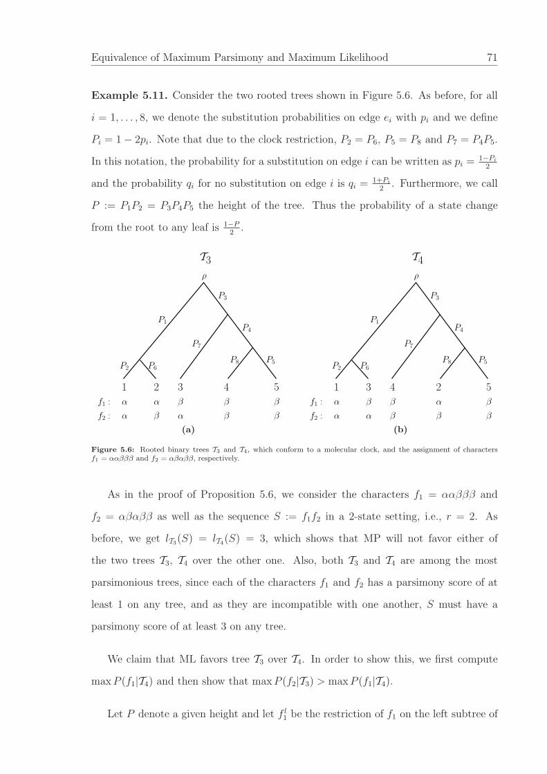
Equivalence of Maximum Parsimony and Maximum Likelihood 71
Example 5.11. Consider the two rooted trees shown in Figure 5.6. As before, for all
i = 1, . . . , 8, we denote the substitution probabilities on edge ei with pi and we define
Pi = 1 − 2pi. Note that due to the clock restriction, P2 = P6, P5 = P8 and P7 = P4P5.
In this notation, the probability for a substitution on edge i can be written as pi = 1−Pi
2
and the probability qi for no substitution on edge i is qi = 1+Pi
2. Furthermore, we call
P := P1P2 = P3P4P5 the height of the tree. Thus the probability of a state change
from the root to any leaf is 1−P2
.
P5
4
β
β
2
αf1 :
α βf2 : α
1 3 5
α β β
ρ
T3
P1
P2 P6
P7
P3
P4
P8
β
(a)
P5
f1 :
α βf2 : β
1 5
α β β
ρ
T4
α
β
β
2
α
3 4
P1
P2 P6
P7
P3
P4
P8
(b)
Figure 5.6: Rooted binary trees T3 and T4, which conform to a molecular clock, and the assignment of charactersf1 = ααβββ and f2 = αβαββ, respectively.
As in the proof of Proposition 5.6, we consider the characters f1 = ααβββ and
f2 = αβαββ as well as the sequence S := f1f2 in a 2-state setting, i.e., r = 2. As
before, we get lT3(S) = lT4(S) = 3, which shows that MP will not favor either of
the two trees T3, T4 over the other one. Also, both T3 and T4 are among the most
parsimonious trees, since each of the characters f1 and f2 has a parsimony score of at
least 1 on any tree, and as they are incompatible with one another, S must have a
parsimony score of at least 3 on any tree.
We claim that ML favors tree T3 over T4. In order to show this, we first compute
max P (f1|T4) and then show that maxP (f2|T3) > max P (f1|T4).
Let P denote a given height and let f l1 be the restriction of f1 on the left subtree of
72 Novel Mathematical Aspects of Phylogenetic Estimation
T4, and f r1 the restriction of f1 on the right subtree of T4. We have
P (f1|T4) = P (f1|T4, ρ = α)P (ρ = α) + P (f1|T4, ρ = β)P (ρ = β)
=1
2P (f l
1|T4, ρ = α)P (f r1 |T4, ρ = α) +
1
2P (f l
1|T4, ρ = β)P (f r1 |T4, ρ = β)
=1
2P (f l
1|T4, ρ = α) (P (f r1 |T4, ρ = α) + P (f r
1 |T4, ρ = β)) , (37)
since P (f l1|T4, ρ = α) = P (f l
1|T4, ρ = β). Moreover, to obtain the ML value, the
two factors P (f l1|T4, ρ = α) and (P (f r
1 |T4, ρ = α) + P (f r1 |T4, ρ = β)) can be maximized
independently.
Evaluating the left factor P (f l1|T4, ρ = α) yields
P (f l1|T4, ρ = α) =
(1 + P1
2
)(1 − P2
2
)(1 + P2
2
)
+
(1 − P1
2
)(1 − P2
2
)(1 + P2
2
)
=1 − P 2
2
4,
which is maximized when P2 takes the minimum possible value. Since P = P1P2 is
given (and fixed), P2 cannot be less than P (otherwise, P1 would have to be more than
1, which is not possible). Therefore,
max P (f l1|T4, ρ = α) =
1 − P 2
4, (38)
and the maximum is obtained when P1 = 1 (since P1P2 = P ). In other words, the
substitution probability p1 = 0, so the left subtree is rooted at ρ by a 0-length edge.
Equivalence of Maximum Parsimony and Maximum Likelihood 73
Analyzing the right factor (P (f r1 |T4, ρ = α) + P (f r
1 |T4, ρ = β)) yields
P (f r1 |T4, ρ = α) + P (f r
1 |T4, ρ = β)
=
(1 + P3
2
)(1 − P4P5
2
)((1 + P4
2
)(1 − P 2
5
4
)
+
(1 − P4
2
)(1 − P 2
5
4
))
+
(1 − P3
2
)(1 + P4P5
2
)((1 − P4
2
)(1 − P 2
5
4
)
+
(1 + P4
2
)(1 − P 2
5
4
))
+
(1 − P3
2
)(1 − P4P5
2
)((1 + P4
2
)(1 − P 2
5
4
)
+
(1 − P4
2
)(1 − P 2
5
4
))
+
(1 + P3
2
)(1 + P4P5
2
)((1 − P4
2
)(1 − P 2
5
4
)
+
(1 + P4
2
)(1 − P 2
5
4
))
=
(1 − P 2
5
4
)
, (39)
which is maximized when P5 is minimum (that is P5 = P ) and P3 = P4 = 1. Combining
Equations (37), (38) and (39) yields
max P (f1|T4) =1
2
(1 − P 2
4
)2
, (40)
obtained by setting P2 = P5 = P and P1 = P3 = P4 = 1, that is, by attaching all leaves
to the root ρ like in a star tree.
It can easily be seen that the right-hand side of Equation (40) is maximized, namely
equal to 132
, when P = 0.
Similarly, maximizing P (f2|T3) yields
max P (f2|T3) =
(1 − P 2
4
)2
, (41)
and this value is obtained by setting P5 = 1 (which corresponds to making the
corresponding edges e5 and e8 short) and as before setting P2 = P , P1 = 1, P3 = 1 and
P4 = P . The right-hand side of Equation (41) assumes its maximum 116
at P = 0.
74 Novel Mathematical Aspects of Phylogenetic Estimation
Equations (40) and (41) imply maxP (f2|T3) > max P (f1|T4) for all fixed values
of P as well as in the limit as P → 0. Note that maxP (f1|T3) = max P (f2|T4). So
altogether we have for the sequence S = f1f2: max P (S|T3) > max P (S|T4). Thus, ML
favors tree T3 over tree T4, whereas both trees are most parsimonious. Therefore, MP
and ML are not equivalent under the constraints of a molecular clock, even when there
is no common mechanism.
As before, we can construct a longer sequence S comprised of k copies of character
f1 and k + c copies of character f2 for some integers k, c > 0. Then k can be chosen
sufficiently large such that ML will favor tree T3 over T4, while T4 is an MP-tree and
T3 is not. Thus, even under the assumption of no common mechanism, MP and ML
choose different sets of trees in this setting.
As in Proposition 5.6, the above example for the binary case subject to a molecular
clock only provides an MP-tree, namely T4, which is not an ML-tree, but it is unclear
whether or not the opposite can occur. However, as both our ternary as well as binary
examples show, it is often possible to modify the examples for bounded substitution
probabilities such that they also provide examples for the clock case. Therefore, we
assume that if such an example exists for the bounded case described in Chapter 5.2,
this might also lead to an example for the restriction induced by a molecular clock.
5.4 Interpretation
Our main objective was to present examples demonstrating that MP and ML may
choose different sets of trees under the Nr-model with no common mechanism when
the substitution probabilities are bounded above by u < 1r
or when a molecular clock
is assumed. Another intention was to give an elementary proof for the equivalence of
MP and ML in the Nr-setting with no common mechanism, as shown by Tuffley and
Steel [44], and thus to make this important result more easily accessible. The main idea
of the proof is basically Corollary 5.4 (which corresponds to Lemma 2 of [44]), which
Equivalence of Maximum Parsimony and Maximum Likelihood 75
states that the maximum likelihood can be obtained at a corner of the k-dimensional
box [0, 1r]k. But as we have shown, for an upper bound u < 1
ron the substitution
probabilities, the approach of assigning probabilities u to those edges on which a most
parsimonious extension g for a given character requires a change and 0 elsewhere, does
not work. This is due to the fact that the maximum of the likelihood function might
occur at a different corner of the box in this case.
Our 4-taxa example employing three character states shows that even if the upper
bound u is arbitrarily close to 1r, we can find a sequence of characters which causes
MP and ML to make conflicting choices. The motivation for our 4-taxa examples was
based on the idea of misleading sequences as defined in Chapter 4. In particular, the
construction idea of the sequences of the present chapter is based on the fact that MP
ignores parsimoniously non-informative characters in any sequence, whereas ML (just
as distance-based methods) does not. We exploited this fact to cause a discrepancy
between MP and ML by taking sufficiently many non-informative characters.
It has been known that there are no binary misleading sequences: If the pairwise
Hamming distances among a set of binary sequences perfectly fit a tree then this tree
is also the perfect phylogeny (see [38], Proposition 7.1.9). But for MP and ML it is
still unknown if under the N2-model with no common mechanism there is a sequence
of binary characters for which these methods make strictly conflicting choices when the
substitution probabilities are bounded above by u < 1r. Our 5-taxa example, which
uses binary characters only, shows that in this setting there are some MP-trees that are
not ML-trees, but we observed that the ML-trees in our examples are also MP-trees –
which means that the equivalence of MP and ML failed but we did not find an example
for strictly conflicting choices in the binary case.
A particularly surprising aspect of our results regards small substitution probabil-
ities, where MP is normally assumed to be justified in the sense of agreement with
ML (see, e.g., [12]): small substitution probabilities or, more precisely, substitution

76 Novel Mathematical Aspects of Phylogenetic Estimation
probabilities subject to an upper bound, are one of the settings that make the equiv-
alence fail – however, we also showed that for a sufficiently small choice of the upper
bound, at least every ML-tree is also an MP-tree (but not vice versa). Moreover, al-
though MP has been proven to agree with ML in the Nr-model under the assumption
of no common mechanism (under no further constraints) our examples show that this
equivalence may fail when the model is changed slightly. Therefore, we conclude that
neither the presence nor the absence of a common mechanism alone can justify MP in
the sense of an MP-ML equivalence. More research could be done on other models of
nucleotide substitution in order to analyze conditions under which ML and MP may
give conflicting results. This might highlight even more differences between MP and
ML.
Chapter 6
Sequence Length Bounds
for Resolving a Deep
Phylogenetic Divergence
There is, after all, one true tree of life, the unique pattern of
evolutionary branchings that actually happened. It exists.
Richard Dawkins
When sequence sites evolve independently under a Markov process along the branches
of a tree T , the sequences observed at the tips contain information concerning the un-
derlying tree. This allows for the tree T to be reconstructed accurately from sufficiently
long sequences, which is the basis of modern molecular systematics [12]. The number
of sites required to accurately reconstruct T depends on how long the edges of the tree
are. More precisely, it depends on the expected number of substitutions on each branch
(edge) e of the tree – which we refer to as the branch length of e (this is the product of
the temporal duration of the branch and the substitution rate).
A number of authors (e.g. [6; 21; 35; 43; 46; 47; 49]) have considered various ways
to quantify the phylogenetic signal in aligned DNA sequences, and to estimate the
sequence length required to reconstruct a phylogenetic tree. Most of these studies have
involved simulations or heuristic approaches, although some analytical bounds have also
been obtained [28; 41]. Typically, these bounds state that if an interior branch length
is very short, or if a terminal (external) branch length is long, then a large number of
sites will be required.
In this chapter, we explore these results further by obtaining bounds that are ex-
pressed purely in terms of the relative sizes of the branch lengths, not their absolute
values. One motivation for our approach is that different genes are known to evolve at
77
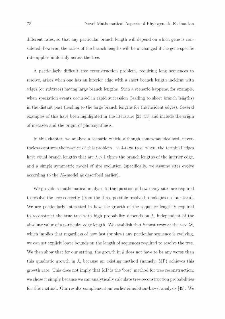
78 Novel Mathematical Aspects of Phylogenetic Estimation
different rates, so that any particular branch length will depend on which gene is con-
sidered; however, the ratios of the branch lengths will be unchanged if the gene-specific
rate applies uniformly across the tree.
A particularly difficult tree reconstruction problem, requiring long sequences to
resolve, arises when one has an interior edge with a short branch length incident with
edges (or subtrees) having large branch lengths. Such a scenario happens, for example,
when speciation events occurred in rapid succession (leading to short branch lengths)
in the distant past (leading to the large branch lengths for the incident edges). Several
examples of this have been highlighted in the literature [23; 33] and include the origin
of metazoa and the origin of photosynthesis.
In this chapter, we analyze a scenario which, although somewhat idealized, never-
theless captures the essence of this problem – a 4-taxa tree, where the terminal edges
have equal branch lengths that are λ > 1 times the branch lengths of the interior edge,
and a simple symmetric model of site evolution (specifically, we assume sites evolve
according to the N2-model as described earlier).
We provide a mathematical analysis to the question of how many sites are required
to resolve the tree correctly (from the three possible resolved topologies on four taxa).
We are particularly interested in how the growth of the sequence length k required
to reconstruct the true tree with high probability depends on λ, independent of the
absolute value of a particular edge length. We establish that k must grow at the rate λ2,
which implies that regardless of how fast (or slow) any particular sequence is evolving,
we can set explicit lower bounds on the length of sequences required to resolve the tree.
We then show that for our setting, the growth in k does not have to be any worse than
this quadratic growth in λ, because an existing method (namely, MP) achieves this
growth rate. This does not imply that MP is the ‘best’ method for tree reconstruction;
we chose it simply because we can analytically calculate tree reconstruction probabilities
for this method. Our results complement an earlier simulation-based analysis [49]. We
Resolving Deep Divergences 79
contrast our results by considering a quite different model of site evolution (the infinite
state model) and establishing that order λ growth in k can sometimes suffice for this
model.
We also extend the approach to more general Markov processes on trees, obtaining
exact, but less explicit lower bounds on k and which involve absolute (rather than rela-
tive) branch lengths. Our arguments are based on standard techniques from probability
theory, such as a Central Limit approximation, and information-theoretic arguments
based on the properties of the Hellinger distance.
6.1 Preliminaries
Consider an unrooted binary phylogenetic tree on four taxa, say 12|34, with branch
length x for the interior edge e5 and λx for the terminal edges e1, . . . , e4, where λ > 1.
This is illustrated in Figure 6.1(a), and the topology of the tree is shown at the top of
Figure 6.1(b). The other two competing topologies (13|24 and 14|23) are also shown
in Figure 6.1(b). Here, branch length refers to the expected number of substitutions
under some continuous time substitution process.
4
3
4
2
4
2
3321
4
1
3
1
2
1
(a) (b)
λx
e2 e3 e4
e5 x
e1
Figure 6.1: (a) The generating tree with interior branch length x and all four terminal branch lengths equal to λx. (b)This tree has the topology 12|34, while the other two binary topologies are 13|24 and 14|23.
80 Novel Mathematical Aspects of Phylogenetic Estimation
Suppose that a sequence of binary characters are generated independently and iden-
tically (i.i.d.) under the N2-model. Although it is the simplest non-trivial Markov
process on a tree, it allows for an exact analysis. Moreover, stochastic results for this
model typically extend to more general finite-state models where an exact analysis is
usually more complex [28], and in Section 6.5 we show how some of our approaches
extend to more general Markov processes.
If we denote the substitution probability on edge ei by P (ei), then for each terminal
edge we have P (ei) = 12(1− exp(−2λx)) while for the central edge e5, we have P (e5) =
12(1 − exp(−2x)). Let θi = 1 − 2P (ei) for i = 1, . . . , 5. Then we can express these five
θi-values in terms of θ := e−2x as follows:
θi = θλ for i = 1, . . . , 4; and θ5 = θ.
Now, if we fix x and let λ grow, or, alternatively, if we fix λx and let x tend to
zero, then the sequence length k required to accurately reconstruct the topology of the
generating tree tends to infinity. Informally, this is because under either of the two
limiting situations described, the three trees in Figure 6.1(b) will (in the limit) give
the same probability distribution on site patterns, and so the three trees will describe
any data equally well. This holds for any tree reconstruction method that treats all
three topologies fairly (if, on the other hand, a method has an a priori preference for a
particular topology, it will perform worse on an alternative topology). Moreover, if λx is
fixed, then k grows at the rate 1x2 as x tends to zero (by Theorem 4.1 of [41]). However,
if we do not fix x or λx in advance, two fundamental questions arise: what is the slowest
rate that k can possibly grow as a function of λ, and does some value of x (dependent
on λ) achieve this rate of growth for a certain tree reconstruction method? We will see
that for the simple scenario described, the answer is that the slowest rate, namely λ2,
can be achieved (up to a constant factor), for example by Maximum Parsimony.
Resolving Deep Divergences 81
6.2 Lower Bounds
The main result of this section is the following theorem.
Theorem 6.1. Suppose k sites evolve i.i.d. under a symmetric 2-state model on some
(unknown) 4-taxa tree that has branch length x on the interior edge and λx on each
terminal edge. Then any method that is able to correctly identify the underlying tree
topology with probability at least 1 − ǫ requires:
k ≥ cǫ · λ2
for any x, where cǫ = 12(1 − 3
2ǫ)2.
To establish this result we require some preliminaries. We begin with a general
information-theoretic bound on the number of i.i.d. observations required to reconstruct
a discrete parameter in a general setting.
Suppose one has a finite set A (e.g., the set of all phylogenetic trees on n taxa), and
each element a ∈ A has an associated probability distribution on a finite set U (e.g.,
the set of all site patterns on n taxa). Suppose we have k observations from U that are
generated independently by the same unknown element a ∈ A. Suppose, furthermore,
that some method M estimates the element of A that generated our observations and
does so correctly with probability at least 1− ǫ (regardless of which element a actually
generated the data). Then we can set a lower bound on k in terms of a stochastic
distance between elements of A.
Definition 6.2 (Hellinger distance). We define the Hellinger distance of two elements
a, a′ ∈ A for a finite set A with associated probability distribution on a finite set U as
follows. If p : U → [0, 1], such that p(u) = pu, and q : U → [0, 1], such that q(u) = qu,
82 Novel Mathematical Aspects of Phylogenetic Estimation
denote the probability distributions induced by a and a′, respectively, then let:
d2H(a, a′) :=
∑
u∈U
(√
pu −√
qu)2 = 2
(
1 −∑
u∈U
√puqu
)
. (42)
Note that the latter equality holds as∑
u∈U
pu =∑
u∈U
qu = 1.
The following result corresponds to Theorem 3.1 and Equation (2.7) in [41].
Lemma 6.3. If there is a subset A′ of A of size m ≥ 2 for which dH(a, a′) ≤ d for all
a, a′ ∈ A′, and some method M correctly identifies each element of A′ with probability
at least 1 − ǫ from k independently generated elements in some set U , then:
k ≥ 1
4(1 − m
m − 1ǫ)2d−2.
In our setting, A will consist of the three binary 4-taxa trees on leaf set {1, 2, 3, 4},
U will consist of the assignment of states to the elements of this leaf set, and m will be
3 (in this chapter) or 2 (in Chapter 6.5).
Let S be the set of possible binary site patterns on {1, 2, 3, 4}. These consist of the
site patterns s1 := ααββ, s2 := αβαβ and s3 := αββα, and five non-informative ones
s4, . . . , s8. Note that pairs of complementary site patterns – for example ααββ and
ββαα – are regarded as equivalent. For any site pattern s ∈ S, let ps = P (s|T1) (and
qs = P (s|T2), respectively) be the probability that the site pattern s is generated on T1
(or T2, respectively). We can express the probabilities ps1 and ps2 in terms of θ = e−2x
by using the Hadamard representation of [16] (see [38], Section 8.6):
ps1 =1
8· (1 + θ1θ2 + θ3θ4 − θ1θ3θ5 − θ2θ3θ5 − θ1θ4θ5 − θ2θ4θ5 + θ1θ2θ3θ4) ,
ps2 =1
8· (1 − θ1θ2 − θ3θ4 + θ1θ3θ5 − θ2θ3θ5 − θ1θ4θ5 + θ2θ4θ5 + θ1θ2θ3θ4) .
Resolving Deep Divergences 83
So here, we have:
ps1 =1
8·(1 + 2 · θ2λ − 4 · θ2λ+1 + θ4λ
), (43)
and
ps2 =1
8·(1 − 2 · θ2λ + θ4λ
)=
1
8
(1 − θ2λ
)2. (44)
To obtain an upper bound on the Hellinger distance, we require a further technical
lemma.
Lemma 6.4. Let γ > 1 and let h(x) = xγ(1−x)(1−xγ)
. Then the supremum of h(x) for x in
the half-open interval [0, 1) equals 1γ.
Proof. Since γ > 1, it can be checked that h′(x) > 0 for all x in (0, 1), and so
supx∈[0,1) h(x) = limx↑1 h(x). By L’Hopital’s rule, we have limx↑1 h(x) = 1γ.
We are now in a position to prove the theorem.
Proof of Theorem 6.1. If any method has a probability of at least 1 − ǫ of correctly
reconstructing each of the three binary trees on four taxa from i.i.d. sequences of
length k then, by Lemma 6.3 with m = 3 we have:
k ≥ (1 − 32ǫ)2
4· d−2
H , (45)
where dH is the maximum Hellinger distance between any two of the three trees. Now,
if each of the three trees has the x, λx combination of branch lengths (for interior and
pending branches, respectively) then, by symmetry, all three of these pairwise Hellinger
distances are equal. Moreover, we claim that:
d−2H ≥ 2λ2, (46)
84 Novel Mathematical Aspects of Phylogenetic Estimation
which together with (45) requires k ≥ cǫλ2 for cǫ = 1
2(1 − 3
2ǫ)2. Thus, it remains to
establish (46).
Wlog. T1 = 12|34 and T2 = 13|24. Now, for all i = 3, . . . , 8, we have psi= qsi
.
Furthermore, ps1 = qs2 and ps2 = qs1 as the given trees are identical except for their
leaf labeling. Consequently, Equation (42) can be simplified as follows:
d2H(T1, T2) = 2
(
1 −8∑
i=1
√psi
qsi
)
= 2
(
1 −8∑
i=3
psi− 2
√ps1ps2
)
, (47)
= 2(1 − (1 − ps1 − ps2) − 2
√ps1ps2
), (48)
= 2(ps1 + ps2 − 2
√ps1ps2
). (49)
Let δ = 12θ2λ(1 − θ). Then ps1 = ps2 + δ, and so Equation (49) can be re-written as:
d2H(T1, T2) = 4ps2
(
1 +δ
2ps2
−√
1 +δ
ps2
)
. (50)
Applying the inequality√
1 + y ≥ 1 + y2− y2
4, for any y > 0, to y = δ
ps2in (50), gives:
d2H(T1, T2) ≤
δ2
ps2
= 2
[θ2λ(1 − θ)
1 − θ2λ
]2
≤ 1
2λ2,
where the last inequality follows by invoking Lemma 6.4 with γ = 2λ, x = θ. This
establishes (46) and thereby completes the proof of the theorem.
6.3 An Upper bound: The Performance of Maximum Parsimony
We now show that the lower bound described above is essentially ‘best possible’ (up to
a constant factor) for the given model, as it can be achieved for a certain choice of x
by a simple tree reconstruction method, namely Maximum Parsimony.
The probability that MP correctly reconstructs the true tree 12|34 will be called
the MP reconstruction probability. Let f(ǫ) denote the one-sided ǫ-critical value for the
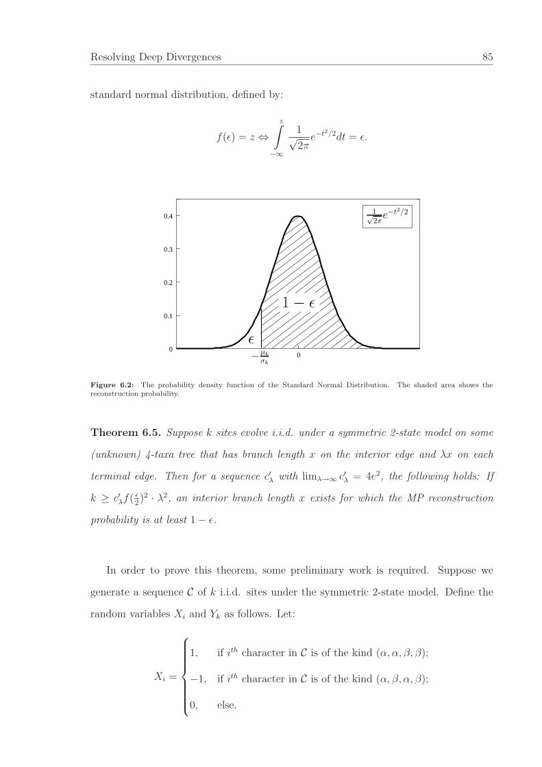
Resolving Deep Divergences 85
standard normal distribution, defined by:
f(ǫ) = z ⇔z∫
−∞
1√2π
e−t2/2dt = ǫ.
0
0.1
0.2
0.3
0.4
0
ǫ
1 − ǫ
−µk
σk
1√2π
e−t2/2
Figure 6.2: The probability density function of the Standard Normal Distribution. The shaded area shows thereconstruction probability.
Theorem 6.5. Suppose k sites evolve i.i.d. under a symmetric 2-state model on some
(unknown) 4-taxa tree that has branch length x on the interior edge and λx on each
terminal edge. Then for a sequence c′λ with limλ→∞ c′λ = 4e2, the following holds: If
k ≥ c′λf( ǫ2)2 · λ2, an interior branch length x exists for which the MP reconstruction
probability is at least 1 − ǫ.
In order to prove this theorem, some preliminary work is required. Suppose we
generate a sequence C of k i.i.d. sites under the symmetric 2-state model. Define the
random variables Xi and Yk as follows. Let:
Xi =
1, if ith character in C is of the kind (α, α, β, β);
−1, if ith character in C is of the kind (α, β, α, β);
0, else.
86 Novel Mathematical Aspects of Phylogenetic Estimation
and let:
Yk =k∑
i=1
Xi. (51)
The probability that MP will favor the tree 12|34 over 13|24 is then P (Yk > 0). We will
exploit the fact that the random variables Xi are i.i.d., and so Yk can be approximated
for large k by a normal distribution with a mean µk and a standard deviation σk. These
two parameters can be easily described (just) in terms of θ, λ and k as follows.
Lemma 6.6.
1. µk = k · [P (X1 = 1) − P (X1 = −1)]
2. σ2k = k ·
[P (X1 = 1) + P (X1 = −1) − [P (X1 = 1) − P (X1 = −1)]2
]
Proof.
1. µk = E(Yk) = E
(k∑
i=1Xi
)
add.=
k∑
i=1E(Xi)
i.i.d.= k · E(X1) =
k·[P (X1 = 1) · 1 + P (X1 = −1) · (−1) + P (X1 = 0) · 0] = k·[P (X1 = 1) − P (X1 = −1)]
2. σ2k = V ar(Yk) = V ar
(k∑
i=1Xi
)
i.i.d.=
k∑
i=1V ar(Xi)
i.i.d.= k · V ar(X1) =
k·[(1 − E(X1))
2 · P (X1 = 1) + (−1 − E(X1))2 · P (X1 = −1) + (0 − E(X1))
2 · P (X1 = 0)]
= k ·[
P (X1 = 1) + P (X1 = −1) − [P (X1 = 1) − P (X1 = −1)]2]
Using this lemma, we can establish the following.
Lemma 6.7.
1. µk = k · 12θ2λ(1 − θ).
2. σ2k = k · 1
4(1 + 2θ4λ+1 − 2θ2λ+1 − θ4λ+2).
3. µk
σk≥
√k · θ2λ(1 − θ).
Resolving Deep Divergences 87
Proof. In the N2-model and the generating tree in Figure 6.1(a), we have:
P (X1 = 1) = ps1 , and P (X1 = −1) = ps2 ,
where ps1 , ps2 were given above in Equations (43) and (44), respectively. Parts (1)
and (2) of the lemma now follow by substitution of the expressions for ps1 , ps2 into the
formulas given by Lemma 6.6(1) and (2), respectively. For Part (3), note that Parts
(1) and (2) imply that
µk
σk
=√
k · Nθ
Dθ
(52)
where Nθ = θ2λ(1− θ); Dθ =√
1 + 2θ4λ+1 − 2θ2λ+1 − θ4λ+2. We now show that Dθ ≤ 1.
We have 1 + 0.5θ2λ+1 ≥ θ2λ and so 2θ2λ+1(1 − θ2λ + 0.5θ2λ+1) ≥ 0. Consequently
1 − 2θ2λ+1(1 − θ2λ + 0.5θ2λ+1) ≤ 1, which implies that D2θ ≤ 1. Part (3) now follows
from (52) by the inequality Dθ ≤ 1.
Proof of Theorem 6.5. Note that the MP reconstruction probability is the probability
that MP will favor the true tree 12|34 over both alternative trees on four taxa, namely
13|24 and 14|23. Recall that the event of the tree 12|34 being favored over 13|24 can be
expressed as P (Yk > 0). The event of 12|34 being favored over 14|23 can be expressed
similarly by defining the random variables Xi and Yk which are analogous to Xi and
Yk, using the character (α, β, β, α) instead of (α, β, α, β). Then, the MP reconstruction
probability can be written as P(
(Yk > 0) ∩ (Yk > 0))
. Let:
Zk =Yk − µk
σk
.
Thus, Zk is the normalized difference of the parsimony score between tree 13|24 and
12|34 for a k i.i.d. characters generated by the tree in Figure 6.1(a). By Lemma 6.7(3)
we have
P (Yk ≤ 0) = P (Zk ≤ −µk
σk
) ≤ P(
Zk ≤ −√
kθ2λ(1 − θ))
. (53)
Now, by symmetry of the branch length of the generating tree in Figure 6.1(a), we have
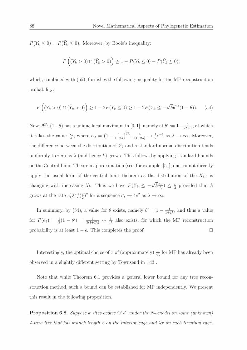
88 Novel Mathematical Aspects of Phylogenetic Estimation
P (Yk ≤ 0) = P (Yk ≤ 0). Moreover, by Boole’s inequality:
P(
(Yk > 0) ∩ (Yk > 0))
≥ 1 − P (Yk ≤ 0) − P (Yk ≤ 0),
which, combined with (55), furnishes the following inequality for the MP reconstruction
probability:
P(
(Yk > 0) ∩ (Yk > 0))
≥ 1 − 2P (Yk ≤ 0) ≥ 1 − 2P (Zk ≤ −√
kθ2λ(1 − θ)). (54)
Now, θ2λ ·(1−θ) has a unique local maximum in [0, 1], namely at θ′ := 1− 12λ+1
, at which
it takes the value αλ
λ, where αλ =
(1 − 1
1+2λ
)2λ · λ(1+2λ)
→ 12e−1 as λ → ∞. Moreover,
the difference between the distribution of Zk and a standard normal distribution tends
uniformly to zero as λ (and hence k) grows. This follows by applying standard bounds
on the Central Limit Theorem approximation (see, for example, [51]; one cannot directly
apply the usual form of the central limit theorem as the distribution of the Xi’s is
changing with increasing λ). Thus we have P (Zk ≤ −√
kαλ
λ) ≤ ǫ
2provided that k
grows at the rate c′λλ2f( ǫ
2)2 for a sequence c′λ → 4e2 as λ → ∞.
In summary, by (54), a value for θ exists, namely θ′ = 1 − 11+2λ
, and thus a value
for P (e5) = 12(1 − θ′) = 1
2(1+2λ)∼ 1
4λalso exists, for which the MP reconstruction
probability is at least 1 − ǫ. This completes the proof.
Interestingly, the optimal choice of x of (approximately) 14λ
for MP has already been
observed in a slightly different setting by Townsend in [43].
Note that while Theorem 6.1 provides a general lower bound for any tree recon-
struction method, such a bound can be established for MP independently. We present
this result in the following proposition.
Proposition 6.8. Suppose k sites evolve i.i.d. under the N2-model on some (unknown)
4-taxa tree that has branch length x on the interior edge and λx on each terminal edge.
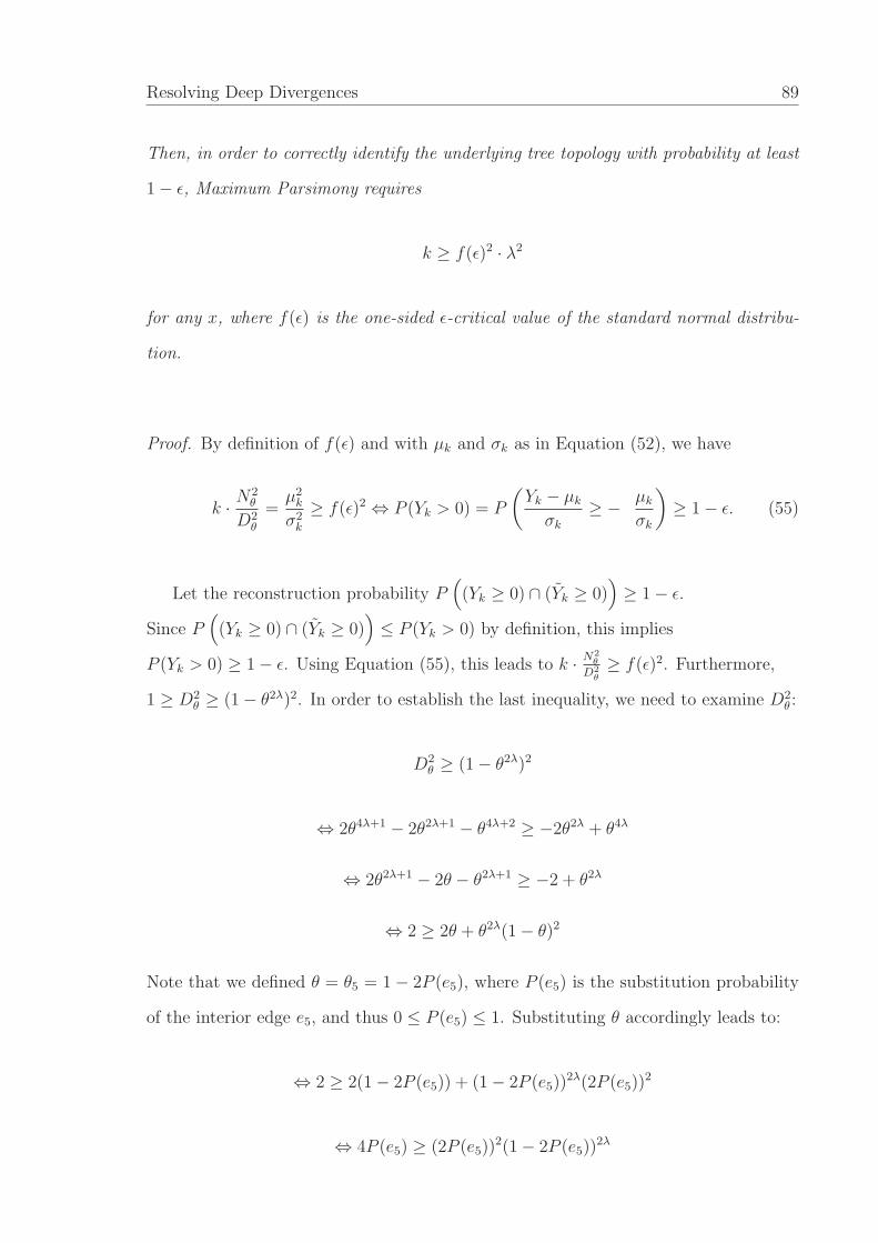
Resolving Deep Divergences 89
Then, in order to correctly identify the underlying tree topology with probability at least
1 − ǫ, Maximum Parsimony requires
k ≥ f(ǫ)2 · λ2
for any x, where f(ǫ) is the one-sided ǫ-critical value of the standard normal distribu-
tion.
Proof. By definition of f(ǫ) and with µk and σk as in Equation (52), we have
k · N2θ
D2θ
=µ2
k
σ2k
≥ f(ǫ)2 ⇔ P (Yk > 0) = P
(Yk − µk
σk
≥ − µk
σk
)
≥ 1 − ǫ. (55)
Let the reconstruction probability P(
(Yk ≥ 0) ∩ (Yk ≥ 0))
≥ 1 − ǫ.
Since P(
(Yk ≥ 0) ∩ (Yk ≥ 0))
≤ P (Yk > 0) by definition, this implies
P (Yk > 0) ≥ 1 − ǫ. Using Equation (55), this leads to k · N2θ
D2θ≥ f(ǫ)2. Furthermore,
1 ≥ D2θ ≥ (1 − θ2λ)2. In order to establish the last inequality, we need to examine D2
θ :
D2θ ≥ (1 − θ2λ)2
⇔ 2θ4λ+1 − 2θ2λ+1 − θ4λ+2 ≥ −2θ2λ + θ4λ
⇔ 2θ2λ+1 − 2θ − θ2λ+1 ≥ −2 + θ2λ
⇔ 2 ≥ 2θ + θ2λ(1 − θ)2
Note that we defined θ = θ5 = 1 − 2P (e5), where P (e5) is the substitution probability
of the interior edge e5, and thus 0 ≤ P (e5) ≤ 1. Substituting θ accordingly leads to:
⇔ 2 ≥ 2(1 − 2P (e5)) + (1 − 2P (e5))2λ(2P (e5))
2
⇔ 4P (e5) ≥ (2P (e5))2(1 − 2P (e5))
2λ
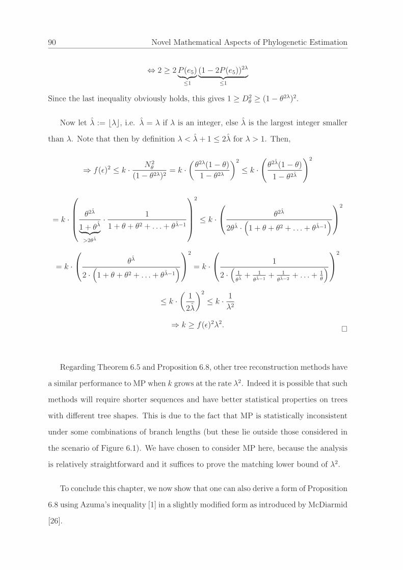
90 Novel Mathematical Aspects of Phylogenetic Estimation
⇔ 2 ≥ 2 P (e5)︸ ︷︷ ︸
≤1
(1 − 2P (e5))2λ
︸ ︷︷ ︸
≤1
Since the last inequality obviously holds, this gives 1 ≥ D2θ ≥ (1 − θ2λ)2.
Now let λ := ⌊λ⌋, i.e. λ = λ if λ is an integer, else λ is the largest integer smaller
than λ. Note that then by definition λ < λ + 1 ≤ 2λ for λ > 1. Then,
⇒ f(ǫ)2 ≤ k · N2θ
(1 − θ2λ)2= k ·
(θ2λ(1 − θ)
1 − θ2λ
)2
≤ k ·(
θ2λ(1 − θ)
1 − θ2λ
)2
= k ·
θ2λ
1 + θλ
︸ ︷︷ ︸
>2θλ
· 1
1 + θ + θ2 + . . . + θλ−1
2
≤ k ·
θ2λ
2θλ ·(
1 + θ + θ2 + . . . + θλ−1)
2
= k ·
θλ
2 ·(
1 + θ + θ2 + . . . + θλ−1)
2
= k ·
1
2 ·(
1
θλ+ 1
θλ−1+ 1
θλ−2+ . . . + 1
θ
)
2
≤ k ·(
1
2λ
)2
≤ k · 1
λ2
⇒ k ≥ f(ǫ)2λ2.
Regarding Theorem 6.5 and Proposition 6.8, other tree reconstruction methods have
a similar performance to MP when k grows at the rate λ2. Indeed it is possible that such
methods will require shorter sequences and have better statistical properties on trees
with different tree shapes. This is due to the fact that MP is statistically inconsistent
under some combinations of branch lengths (but these lie outside those considered in
the scenario of Figure 6.1). We have chosen to consider MP here, because the analysis
is relatively straightforward and it suffices to prove the matching lower bound of λ2.
To conclude this chapter, we now show that one can also derive a form of Proposition
6.8 using Azuma’s inequality [1] in a slightly modified form as introduced by McDiarmid
[26].
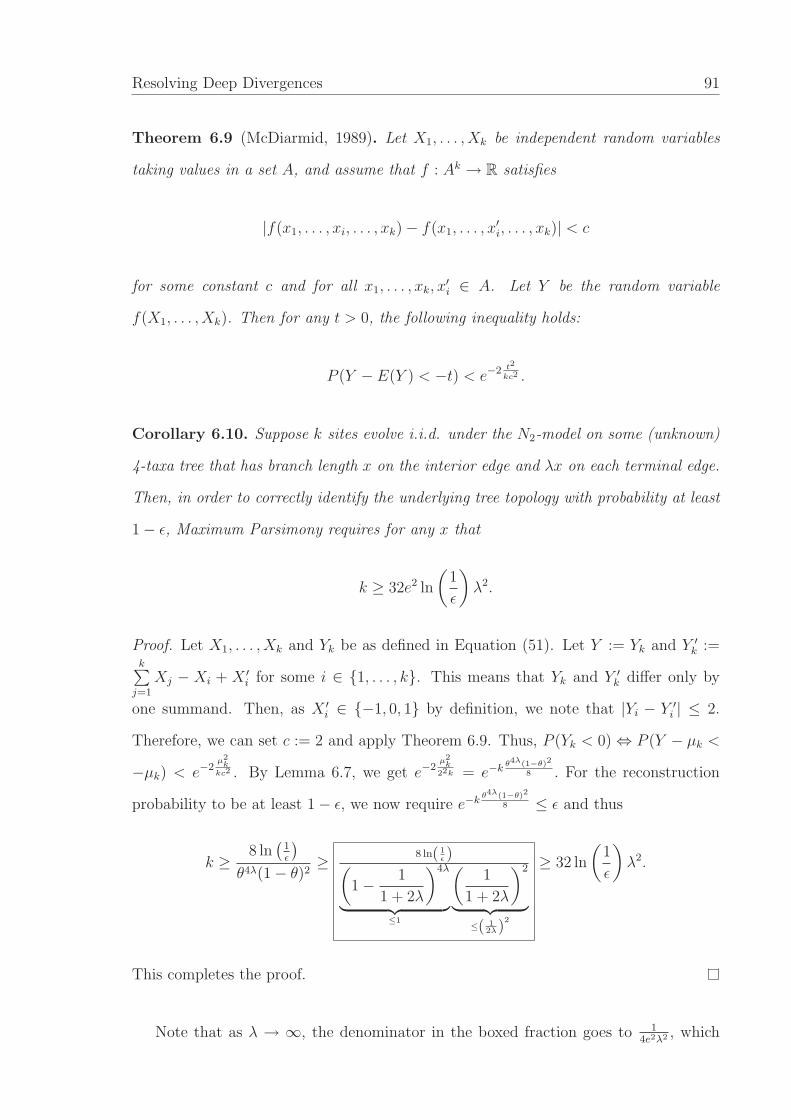
Resolving Deep Divergences 91
Theorem 6.9 (McDiarmid, 1989). Let X1, . . . , Xk be independent random variables
taking values in a set A, and assume that f : Ak → R satisfies
|f(x1, . . . , xi, . . . , xk) − f(x1, . . . , x′i, . . . , xk)| < c
for some constant c and for all x1, . . . , xk, x′i ∈ A. Let Y be the random variable
f(X1, . . . , Xk). Then for any t > 0, the following inequality holds:
P (Y − E(Y ) < −t) < e−2 t2
kc2 .
Corollary 6.10. Suppose k sites evolve i.i.d. under the N2-model on some (unknown)
4-taxa tree that has branch length x on the interior edge and λx on each terminal edge.
Then, in order to correctly identify the underlying tree topology with probability at least
1 − ǫ, Maximum Parsimony requires for any x that
k ≥ 32e2 ln
(1
ǫ
)
λ2.
Proof. Let X1, . . . , Xk and Yk be as defined in Equation (51). Let Y := Yk and Y ′k :=
k∑
j=1
Xj − Xi + X ′i for some i ∈ {1, . . . , k}. This means that Yk and Y ′
k differ only by
one summand. Then, as X ′i ∈ {−1, 0, 1} by definition, we note that |Yi − Y ′
i | ≤ 2.
Therefore, we can set c := 2 and apply Theorem 6.9. Thus, P (Yk < 0) ⇔ P (Y − µk <
−µk) < e−2µ2
kkc2 . By Lemma 6.7, we get e−2
µ2k
22k = e−kθ4λ(1−θ)2
8 . For the reconstruction
probability to be at least 1 − ǫ, we now require e−kθ4λ(1−θ)2
8 ≤ ǫ and thus
k ≥ 8 ln(
1ǫ
)
θ4λ(1 − θ)2≥ 8 ln( 1
ǫ )(
1 − 1
1 + 2λ
)4λ
︸ ︷︷ ︸≤1
(1
1 + 2λ
)2
︸ ︷︷ ︸
≤( 12λ)
2
≥ 32 ln
(1
ǫ
)
λ2.
This completes the proof.
Note that as λ → ∞, the denominator in the boxed fraction goes to 14e2λ2 , which
92 Novel Mathematical Aspects of Phylogenetic Estimation
gives k ≥ 32e2 ln(
1ǫ
)λ2. So in the limit, the term in place of c′λ is larger by a factor
of 8 than suggested by the Central Limit Theorem, but the advantage of the Azuma
approach as opposed to the CLT is that it is non-asymptotic and therefore valid for
any given finite k.
6.4 The Performance of MP under the Random Cluster Model
We now consider Markov processes in which the state space is countably infinite, and
where a substitution is always to a new state. In particular, we consider the following
random process on a phylogenetic tree T . For each edge e ∈ E(T ), let a map p : e 7→
p(e), where p(e) denotes a probability, be given (and let all p(e)’s be independent). Then
cut this edge with probability p(e) (or leave it intact with probability 1 − p(e)). The
resulting disconnected graph partitions the vertex set V (T ) into non-empty components
according to the equivalence relation that u ∼ v if u and v are in the same component.
This process thus generates random partitions of V (T ), and thereby of X. We call
the resulting probability distribution on partitions of X the random cluster model for
homoplasy-free evolution with parameters (T , p). For more information on this model,
the reader is referred to [27].
For the random cluster model, the situation regarding sequence length requirements
is quite different from that of the N2-model described in the previous chapter. In this
case, the required sequence length need only grow at the rate λ (not λ2), as the following
result shows.
Proposition 6.11. Suppose k sites evolve i.i.d. under a random cluster model on some
(unknown) 4-taxa tree that has branch length x on the interior edge and λx on each
terminal edge. Then, for a constant C ′ǫ which depends just on ǫ, the following holds: If
k ≥ C ′ǫ ·λ, then an x exists for which the MP reconstruction probability is at least 1− ǫ.
Proof. In the random cluster model, the probability of a substitution event on an edge e
Resolving Deep Divergences 93
can be written as P (e) = 1− exp(−l) where l is the expected number of changes on the
edge (the branch length). Now, the random cluster model generates only characters
that are homoplasy-free on the generating tree; thus MP will return the generating
tree from a sequence of characters, provided this tree is the only one on which those
characters are homoplasy-free. For a tree with topology 12|34, this will occur precisely
if at least one of the k characters generated assigns taxa 1, 2 a shared state, and taxa
3, 4 a second shared state that is different to that assigned to 1, 2. The probability Q
that any given character generated by the tree in Figure 6.1(a) has this property is
given by:
Q = P (e5)4∏
i=1
(1 − P (ei)) = (1 − e−x)e−4λx.
Moreover, if k ≥ log( 1ǫ )
Qthen 1−(1−Q)k ≥ 1−ǫ (using the inequality − log(1−Q) ≥ Q).
Consequently, MP will correctly reconstruct the generating tree with probability at least
1 − ǫ provided that:
k ≥ log(ǫ−1) · (1 − e−x)−1e4λx. (56)
Taking x = 14λ
we have (1 − e−x)−1e4λx ∼ 4eλ, which, in view of Equation (56),
establishes the result.
6.5 Lower Bounds for More General Models
In this chapter we derive a lower bound on the sequence length required for tree recon-
struction, for a much wider range of Markov processes. However, unlike the previous
chapters our bound is expressed in terms of the absolute branch lengths (or bounds
on these) rather than in terms of ratios, and it involves constants that depend on the
details of the model.
We first derive a general lemma. Consider any continuous-time, stationary and
reversible Markov process. Let S denote its state space (thus, in previous sections
S = {α, β}), and let S = S4. Let T1 and T2 be two topologically distinct 4-taxa trees.
94 Novel Mathematical Aspects of Phylogenetic Estimation
Suppose that the branch lengths of T1 are arbitrary, and that each edge of T2 has the
corresponding interior or pendant branch length specified by T1 (where the pendant edge
incident with leaf i in T1 corresponds to the pendant edge incident with leaf i in T2).
For s = (s1, s2, s3, s4) ∈ S, let ps (respectively qs) denote the probability of generating
s at the tips of T1 (respectively T2). Let p′s (respectively q′s) denote the conditional
probability of generating s at the tips of T1 (respectively T2) given that a substitution
has occurred on the central edge of T1 (respectively T2), and let Ds := q′s − p′s. Then
we have the following result.
Lemma 6.12.
d2H(T1, T2) ≤ l2 ·
∑
s∈S
D2s
ps
where l denotes the branch length of the interior edge of T1.
Proof. Let τ denote the probability that a substitution occurs on the interior edge
of T1, and let p0s (respectively q0
s) denote the conditional probability of generating s
on T1 (respectively T2) given that no substitution occurs on the interior edge of T1
(respectively T2). By the law of total probability we have:
ps = (1 − τ) · p0s + τ · p′s
and
qs = (1 − τ) · q0s + τ · q′s.
Moreover, the assumptions on the correspondence between branch lengths of T1 and T2
imply that p0s = q0
s for all s ∈ S and so:
qs − ps = τ(q′s − p′s) = τDs.
Resolving Deep Divergences 95
Now,
d2H(T1, T2) = 2(1 −
∑
s∈S
√psqs) = 2
(
1 −∑
s∈S
ps
√
1 +τDs
ps
)
.
Applying the inequality√
1 + y ≥ 1+ y2− y2
2(for all y ≥ −1) to y = τDs
ps(and observing
that y ≥ −1 since qs ≥ 0), we obtain:
d2H(T1, T2) ≤ 2
(
1 −∑
s
ps
(
1 + τDs
2ps
− τ 2 D2s
2ps
))
.
Now,∑
s ps = 1, and∑
s Ds = 0 (since∑
s q′s =∑
s p′s = 1) and so this last inequality
reduces to:
d2H(T1, T2) ≤ τ 2 ·
∑
s∈S
D2s
ps
. (57)
Furthermore, τ = P (N > 0), where N is the number of substitutions occurring on the
interior edge of T1. However, P (N > 0) ≤ E(N); that is, τ ≤ l, which, together with
(57), provides the inequality stated in the lemma.
We now apply this lemma to a slightly more restricted class of Markov processes to
obtain the main result of this section.
Theorem 6.13. Suppose k sites evolve i.i.d. under a finite-state, stationary and re-
versible continuous-time Markov process in which each state is accessible from any other
state. Let l0 be any strictly positive value. Consider this process on some (unknown)
4-taxa tree that has branch length at most l on the interior edge and at least L ≥ l0 on
each terminal edge. Then any method that is able to correctly identify with probability
at least 1 − ǫ the underlying tree topology given these restriction requires:
k ≥ C
4(1 − 2ǫ)2 · ecL
l2
where c and C are positive constants that depend only on R (the rate matrix for the
process) and l0.
96 Novel Mathematical Aspects of Phylogenetic Estimation
Proof. We exploit the fact that any Markov process of the type described converges to
its unique stationary distribution at an exponential rate (see, for example, Theorem
8.3 of [34]). Let π(s) denote the stationary probability of s under the model. For
j = 1, . . . , 4, let p(j) ∈ {u, v} be the end of the interior edge uv of T1 that is adjacent
to leaf j (we may assume p(1) = p(2) = u; p(3) = p(4) = v), and let Sp(j) denote the
random state present at that vertex under the model. Then for any sj, s′j ∈ S there
exist positive constants A, a (dependent on R) for which:
|P (Sj = sj|Sp(j) = s′j) − π(sj)| ≤ Ae−aLj (58)
([34], Theorem 8.3), where Lj denotes the branch length of the edge incident with leaf
j. For s = (s1, s2, s3, s4) ∈ S = S4, let
πs =4∏
j=1
π(sj).
For s′s′′ ∈ S let p′(s′, s′′) denote the probability of generating state s′ at u and the state
s′′ at v given that at least one substitution occurs on the edge uv. Then, by the Markov
assumption, and recalling the definition of p′s from Lemma 6.12, we have:
p′s =∑
(s′,s′′)∈S2
p′(s′, s′′) ·2∏
j=1
P (Sj = sj|Su = s′) ·4∏
j=3
P (Sj = sj|Sv = s′′). (59)
Combining (58) and (59), there exist positive constants B, b (dependent only on R)
such that:
|p′s − πs| ≤ Be−bL (60)
for all s ∈ S (recall that L ≤ Lj for all j). Now, consider tree T2 which has branch
lengths that correspond to those in T1 (as in Lemma 6.12). Then we also have:
|q′s − πs| ≤ Be−bL (61)
Resolving Deep Divergences 97
for all s ∈ S. Combining (60) and (61) using the triangle inequality gives:
|Ds| = |qs − ps| ≤ 2Be−bL. (62)
Moreover, since Lj ≥ l0 (for all j) and each state is accessible from any other state, we
have ps ≥ δ (for some δ > 0 dependent only on R and l0). Combining this with (62)
gives the following inequality, for all s ∈ S:
D2s
ps
≤ (4B2/δ)e−2bL. (63)
The theorem now follows from Lemma 6.12 and Lemma 6.3 (with m = 2).
6.6 Interpretation
In this chapter we have provided precise results for a specific and simple model (the N2-
model), along with less explicit results for more general Markov processes (and phrased
in terms of absolute rather than relative branch lengths). The aim was to determine
rigorous bounds on the sequence length required for resolving a deep divergence, which
may shed light on debates as to whether some early radiations might be fundamentally
unresolvable on the basis of current models and data.
Of course, in applications, other phenomena (such as lineage sorting, sequencing
errors, substitution model mis-specification, misalignment of sequences and alignment
artifacts [32] and so forth) may further impede phylogenetic reconstruction. These
errors are unlikely to help the tree reconstruction if our bound shows it is impossible
even when the ideal model assumptions hold. We have seen that some models require
significantly fewer characters for resolving a tree – in particular this holds for the random
cluster model, and it is possible that new types of genomic data (involving rare genomic
events where homoplasy is unlikely) can be described by these and related processes
that preserve more phylogenetic signal regarding distant evolutionary divergences.

98 Novel Mathematical Aspects of Phylogenetic Estimation
One limitation concerning our bounds is that they apply to pure Markov processes,
in which each character evolves according to the same process. In molecular biology, a
common assumption is that there is a distribution of rates across sites, in which each
site evolves at a rate (selected independently from some fixed distribution) that acts
as a multiplier for all the branch lengths in the tree (see e.g. [12; 38]). It would be
interesting to extend the analysis in the last section to these models to obtain a lower
bound on k analogous to Theorem 6.13.
Chapter 7
Expected Anomalies
in the Fossil Record
Why has not anyone seen that fossils alone gave birth to a the-
ory about the formation of the earth, that without them, no one
would have ever dreamed that there were successive epochs in the
formation of the globe?
Georges Cuvier
Since Darwin’s book On the Origin of Species by Means of Natural Selection, or the
Preservation of Favoured Races in the Struggle for Life [7], there has been much debate
about the evidence for continuous evolution from a universal common ancestor. Initially,
Darwin only assumed the relatedness of the majority of species, not of all of them.
Later, however, he came to the view that because of the similarities of all existing
species, there could only be one ‘root’ and one ‘tree of life’ [39]. All species have
descended from this common ancestor and indications for their gradual evolution have
been sought in the fossil record ever since. Usually, the improbability of fossilization
or of finding existing fossils was put forward as the standard answer to the question of
why there are so many ‘gaps’ in the fossil record. Such gaps have become popularly
referred to as ‘missing links’, i.e., missing intermediates between taxa existing either
today or as fossils.
Of course, the existence of gaps is in some sense inevitable: every new link gives
rise to two new gaps, since evolution is generally a continuous process whereas fossil
discovery will always remain discontinuous. Moreover, a patchy fossil record is not
necessarily evidence against evolution from a common ancestor through a continuous
series of intermediates – indeed, in a recent approach, Elliott Sober applied simple
probabilistic arguments to conclude that the existence of some intermediates provides
99
100 Novel Mathematical Aspects of Phylogenetic Estimation
a stronger support for evolution than the non-existence of any (or some) intermediates
could ever provide for a hypothesis of separate ancestry [39]. Moreover, some lineages
appear to be densely sampled, whereas of others only few fossiliferous horizons are
known [37]. This problem has been well investigated and statistical models have been
developed to master it (see e.g. [25], [24]), [42]).
In this chapter, we suggest a further argument that may help explain missing links
in the fossil record. Suppose that three fossils can be dated back to three different times.
Can we really expect that a fossil from the intermediate time will appear (morphologi-
cally) to be an ‘intermediate’ of the other two fossils? We will explore this question via
a simple stochastic model.
In order to develop this model, we first state some assumptions: firstly, we will
consider that we are sampling fossil taxa of closely related organisms and which differ
in a number of morphological characteristics. We assume this group of taxa has evolved
in a ‘treelike’ fashion from some common ancestor; that is, there is an underlying
phylogenetic tree, and the taxa are randomly sampled from points on the branches of
this tree for given times. It is also necessary to say how morphological divergence might
be related to time, as this is important for deciding whether a taxon is an intermediate
or not. We will introduce two different interpretations for the degree of morphological
divergence: in Chapter 7.2, we assume that fossils connected by short paths in the
underlying phylogenetic tree are closely related, whereas fossils connected by a longer
path are not as closely related. In Chapter 7.3, we will explain a biological drawback of
this approach and analyze a more cladistic setting to overcome this problem. We will
show, however, that for both approaches the main result does not change; namely, that
it is possible that fossils from an intermediate time can, for certain trees and times,
be expected to be less related to the first and the last sample than the latter two to
one another. This surprising and counterintuitive result may help explain some of the
‘gaps’ in the fossil record.
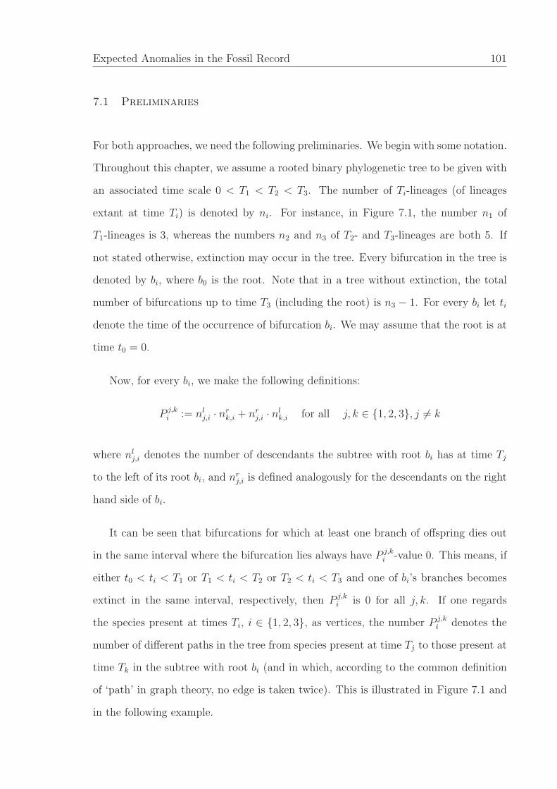
Expected Anomalies in the Fossil Record 101
7.1 Preliminaries
For both approaches, we need the following preliminaries. We begin with some notation.
Throughout this chapter, we assume a rooted binary phylogenetic tree to be given with
an associated time scale 0 < T1 < T2 < T3. The number of Ti-lineages (of lineages
extant at time Ti) is denoted by ni. For instance, in Figure 7.1, the number n1 of
T1-lineages is 3, whereas the numbers n2 and n3 of T2- and T3-lineages are both 5. If
not stated otherwise, extinction may occur in the tree. Every bifurcation in the tree is
denoted by bi, where b0 is the root. Note that in a tree without extinction, the total
number of bifurcations up to time T3 (including the root) is n3 − 1. For every bi let ti
denote the time of the occurrence of bifurcation bi. We may assume that the root is at
time t0 = 0.
Now, for every bi, we make the following definitions:
P j,ki := nl
j,i · nrk,i + nr
j,i · nlk,i for all j, k ∈ {1, 2, 3}, j 6= k
where nlj,i denotes the number of descendants the subtree with root bi has at time Tj
to the left of its root bi, and nrj,i is defined analogously for the descendants on the right
hand side of bi.
It can be seen that bifurcations for which at least one branch of offspring dies out
in the same interval where the bifurcation lies always have P j,ki -value 0. This means, if
either t0 < ti < T1 or T1 < ti < T2 or T2 < ti < T3 and one of bi’s branches becomes
extinct in the same interval, respectively, then P j,ki is 0 for all j, k. If one regards
the species present at times Ti, i ∈ {1, 2, 3}, as vertices, the number P j,ki denotes the
number of different paths in the tree from species present at time Tj to those present at
time Tk in the subtree with root bi (and in which, according to the common definition
of ‘path’ in graph theory, no edge is taken twice). This is illustrated in Figure 7.1 and
in the following example.
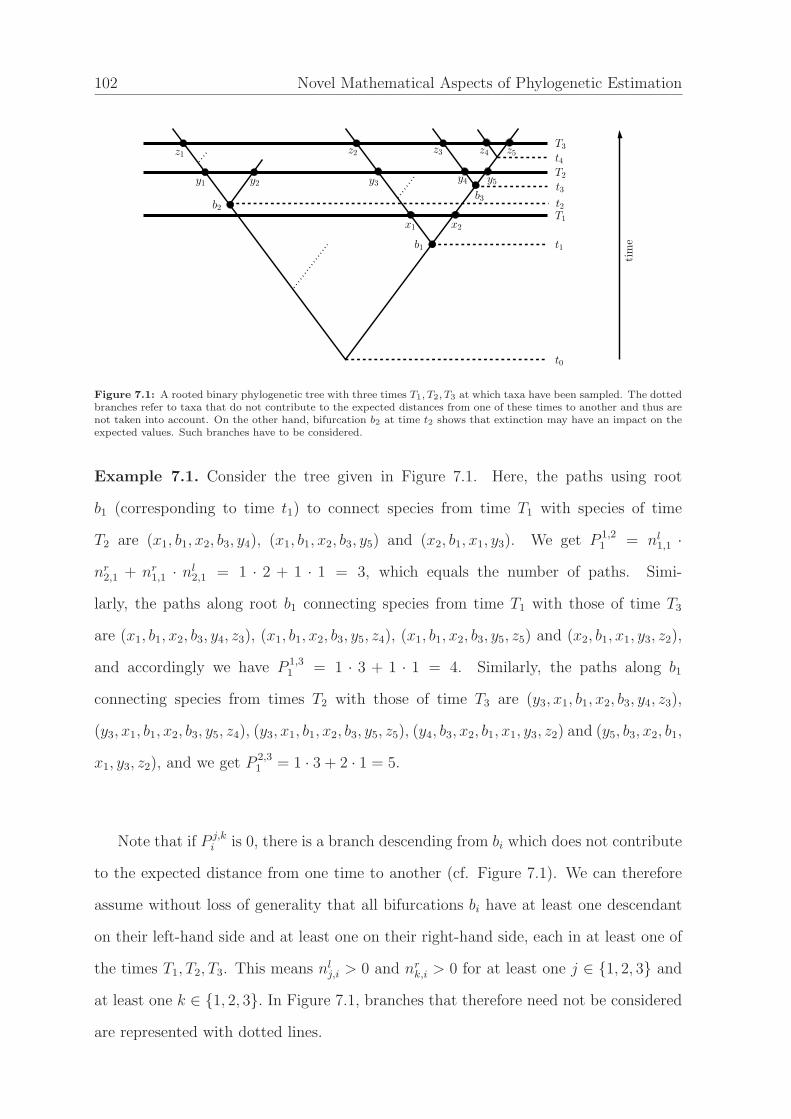
102 Novel Mathematical Aspects of Phylogenetic Estimation
T3
T2
T1
t1
t0
tim
e
t4
t3
b2
y2y1
z1z5
y5y4y3
x2x1
b1
t2
z4z3z2
b3
Figure 7.1: A rooted binary phylogenetic tree with three times T1, T2, T3 at which taxa have been sampled. The dottedbranches refer to taxa that do not contribute to the expected distances from one of these times to another and thus arenot taken into account. On the other hand, bifurcation b2 at time t2 shows that extinction may have an impact on theexpected values. Such branches have to be considered.
Example 7.1. Consider the tree given in Figure 7.1. Here, the paths using root
b1 (corresponding to time t1) to connect species from time T1 with species of time
T2 are (x1, b1, x2, b3, y4), (x1, b1, x2, b3, y5) and (x2, b1, x1, y3). We get P 1,21 = nl
1,1 ·
nr2,1 + nr
1,1 · nl2,1 = 1 · 2 + 1 · 1 = 3, which equals the number of paths. Simi-
larly, the paths along root b1 connecting species from time T1 with those of time T3
are (x1, b1, x2, b3, y4, z3), (x1, b1, x2, b3, y5, z4), (x1, b1, x2, b3, y5, z5) and (x2, b1, x1, y3, z2),
and accordingly we have P 1,31 = 1 · 3 + 1 · 1 = 4. Similarly, the paths along b1
connecting species from times T2 with those of time T3 are (y3, x1, b1, x2, b3, y4, z3),
(y3, x1, b1, x2, b3, y5, z4), (y3, x1, b1, x2, b3, y5, z5), (y4, b3, x2, b1, x1, y3, z2) and (y5, b3, x2, b1,
x1, y3, z2), and we get P 2,31 = 1 · 3 + 2 · 1 = 5.
Note that if P j,ki is 0, there is a branch descending from bi which does not contribute
to the expected distance from one time to another (cf. Figure 7.1). We can therefore
assume without loss of generality that all bifurcations bi have at least one descendant
on their left-hand side and at least one on their right-hand side, each in at least one of
the times T1, T2, T3. This means nlj,i > 0 and nr
k,i > 0 for at least one j ∈ {1, 2, 3} and
at least one k ∈ {1, 2, 3}. In Figure 7.1, branches that therefore need not be considered
are represented with dotted lines.
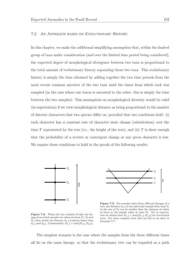
Expected Anomalies in the Fossil Record 103
7.2 An Approach based on Evolutionary History
In this chapter, we make the additional simplifying assumption that, within the limited
group of taxa under consideration (and over the limited time period being considered),
the expected degree of morphological divergence between two taxa is proportional to
the total amount of evolutionary history separating those two taxa. This evolutionary
history is simply the time obtained by adding together the two time periods from the
most recent common ancestor of the two taxa until the times from which each was
sampled (in the case where one taxon is ancestral to the other, this is simply the time
between the two samples). This assumption on morphological diversity would be valid
(in expectation) if we view morphological distance as being proportional to the number
of discrete characters that two species differ on, provided that two conditions hold: (i)
each character has a constant rate of character state change (substitution) over the
time T represented by the tree (i.e., the height of the tree), and (ii) T is short enough
that the probability of a reverse or convergent change at any given character is low.
We require these conditions to hold in the proofs of the following results.
time
T3
T2
T1
Figure 7.2: When the tree consists of only one lin-eage from which samples are taken at times T1, T2 andT3, then clearly the distance d1,3 is always larger thand1,2 and d2,3. Consequently, E1,3 > max{E1,2, E2,3}.
time
T3
T2
T1
Figure 7.3: For samples taken from different lineages of atree, the distance d1,3 of one particular sample from time T1
to the one of T3 can be smaller than the distance of eitherof them to the sample taken at time T2. Yet in expecta-tion we always have E1,3 > max{E1,2, E2,3} for two-branchtrees. For more complex trees this can fail as we show inExample 7.7.
The simplest scenario is the case where the samples from the three different times
all lie on the same lineage, so that the evolutionary tree can be regarded as a path
104 Novel Mathematical Aspects of Phylogenetic Estimation
(cf. Figure 7.2). In this case, the path distance (and hence expected morphological
distance) between the outer two fossils is always larger than the distance that either
of them has from the fossil sampled from an intermediate time. But for samples that
straddle bifurcations in a tree, it is quite easy to imagine how this intermediacy could
fail; for example, if the two outer taxa lie on one branch of the tree and the fossil from
the intermediate time lies on another branch far away (cf. Figure 7.3). But this example
might be unlikely to occur, and indeed we will see that if sampling is uniform across the
tree at any given time, in expectation the morphological distances remain intermediate
even for this case (cf. Figure 7.3). Yet for more complex trees, this expected outcome
can fail, and perhaps most surprisingly, the distance between the earliest and latest
sample can, in expectation, be the smallest of the three distances in certain extreme
cases.
Thus, in order to make general statements, we will consider the expected degree
of relatedness of fossils sampled randomly from given times. Our results will depend
solely on the tree shape (including branch lengths) of the underlying tree and the chosen
times.
In the sampling, select uniformly at random one of the Ti-lineages as well as one of
the Tj-lineages to get the expected length Ei,j of the path connecting a lineage at time
Ti with one at time Tj in the underlying phylogenetic tree. Then, the expectation that a
fossil from the intermediate time T2 also will be an intermediate taxon of two taxa taken
from T1 and T3, respectively, refers to the assumption that E1,3 > max{E1,2, E2,3}. We
will show in the following lemma that this last inequality can fail and describe the
precise condition for this to occur. Moreover, we later show that E1,3 can be strictly
smaller (!) than both E1,2 and E2,3 - that is the temporally most distant samples can,
on average, be more similar than the temporally intermediate sample is to either of the
two.
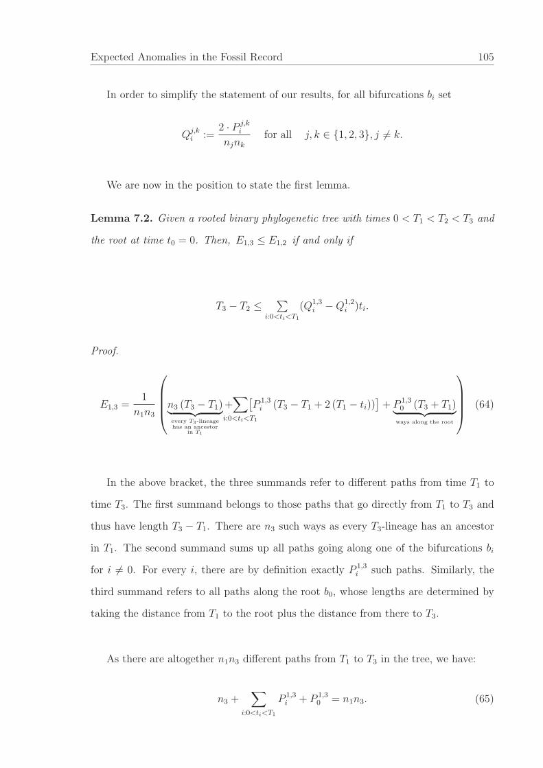
Expected Anomalies in the Fossil Record 105
In order to simplify the statement of our results, for all bifurcations bi set
Qj,ki :=
2 · P j,ki
njnk
for all j, k ∈ {1, 2, 3}, j 6= k.
We are now in the position to state the first lemma.
Lemma 7.2. Given a rooted binary phylogenetic tree with times 0 < T1 < T2 < T3 and
the root at time t0 = 0. Then, E1,3 ≤ E1,2 if and only if
T3 − T2 ≤∑
i:0<ti<T1
(Q1,3i − Q1,2
i )ti.
Proof.
E1,3 =1
n1n3
n3 (T3 − T1)︸ ︷︷ ︸every T3-lineagehas an ancestor
in T1
+∑
i:0<ti<T1
[P 1,3
i (T3 − T1 + 2 (T1 − ti))]+ P 1,3
0 (T3 + T1)︸ ︷︷ ︸
ways along the root
(64)
In the above bracket, the three summands refer to different paths from time T1 to
time T3. The first summand belongs to those paths that go directly from T1 to T3 and
thus have length T3 − T1. There are n3 such ways as every T3-lineage has an ancestor
in T1. The second summand sums up all paths going along one of the bifurcations bi
for i 6= 0. For every i, there are by definition exactly P 1,3i such paths. Similarly, the
third summand refers to all paths along the root b0, whose lengths are determined by
taking the distance from T1 to the root plus the distance from there to T3.
As there are altogether n1n3 different paths from T1 to T3 in the tree, we have:
n3 +∑
i:0<ti<T1
P 1,3i + P 1,3
0 = n1n3. (65)
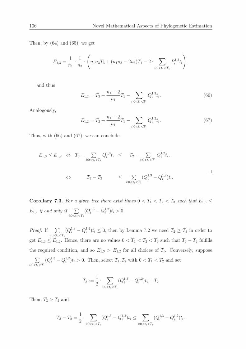
106 Novel Mathematical Aspects of Phylogenetic Estimation
Then, by (64) and (65), we get
E1,3 =1
n1
· 1
n3
·(
n1n3T3 + (n1n3 − 2n3)T1 − 2 ·∑
i:0<ti<T1
P 1,3i ti
)
,
and thus
E1,3 = T3 +n1 − 2
n1
T1 −∑
i:0<ti<T1
Q1,3i ti. (66)
Analogously,
E1,2 = T2 +n1 − 2
n1
T1 −∑
i:0<ti<T1
Q1,2i ti. (67)
Thus, with (66) and (67), we can conclude:
E1,3 ≤ E1,2 ⇔ T3 −∑
i:0<ti<T1
Q1,3i ti ≤ T2 −
∑
i:0<ti<T1
Q1,2i ti,
⇔ T3 − T2 ≤ ∑
i:0<ti<T1
(Q1,3i − Q1,2
i )ti.
Corollary 7.3. For a given tree there exist times 0 < T1 < T2 < T3 such that E1,3 ≤
E1,2 if and only if∑
i:0<ti<T1
(Q1,3i − Q1,2
i )ti > 0.
Proof. If∑
i:0<ti<T1
(Q1,3i − Q1,2
i )ti ≤ 0, then by Lemma 7.2 we need T2 ≥ T3 in order to
get E1,3 ≤ E1,2. Hence, there are no values 0 < T1 < T2 < T3 such that T3 − T2 fulfills
the required condition, and so E1,3 > E1,2 for all choices of Ti. Conversely, suppose∑
i:0<ti<T1
(Q1,3i − Q1,2
i )ti > 0. Then, select T1, T2 with 0 < T1 < T2 and set
T3 :=1
2·∑
i:0<ti<T1
(Q1,3i − Q1,2
i )ti + T2
Then, T3 > T2 and
T3 − T2 =1
2·∑
i:0<ti<T1
(Q1,3i − Q1,2
i )ti ≤∑
i:0<ti<T1
(Q1,3i − Q1,2
i )ti.
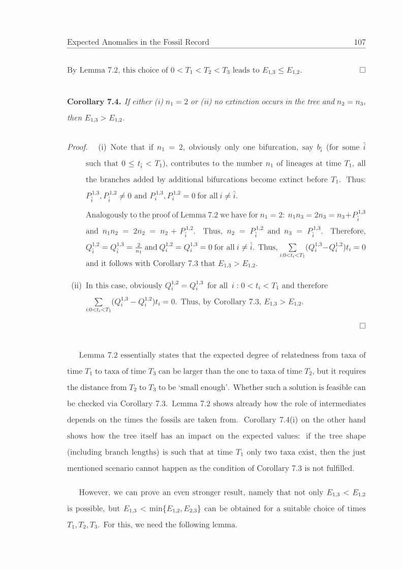
Expected Anomalies in the Fossil Record 107
By Lemma 7.2, this choice of 0 < T1 < T2 < T3 leads to E1,3 ≤ E1,2.
Corollary 7.4. If either (i) n1 = 2 or (ii) no extinction occurs in the tree and n2 = n3,
then E1,3 > E1,2.
Proof. (i) Note that if n1 = 2, obviously only one bifurcation, say bi (for some i
such that 0 ≤ ti < T1), contributes to the number n1 of lineages at time T1, all
the branches added by additional bifurcations become extinct before T1. Thus:
P 1,3
i, P 1,2
i6= 0 and P 1,3
i , P 1,2i = 0 for all i 6= i.
Analogously to the proof of Lemma 7.2 we have for n1 = 2: n1n3 = 2n3 = n3+P 1,3
i
and n1n2 = 2n2 = n2 + P 1,2
i. Thus, n2 = P 1,2
iand n3 = P 1,3
i. Therefore,
Q1,2
i= Q1,3
i= 2
n1and Q1,2
i = Q1,3i = 0 for all i 6= i. Thus,
∑
i:0<ti<T1
(Q1,3i −Q1,2
i )ti = 0
and it follows with Corollary 7.3 that E1,3 > E1,2.
(ii) In this case, obviously Q1,2i = Q1,3
i for all i : 0 < ti < T1 and therefore∑
i:0<ti<T1
(Q1,3i − Q1,2
i )ti = 0. Thus, by Corollary 7.3, E1,3 > E1,2.
Lemma 7.2 essentially states that the expected degree of relatedness from taxa of
time T1 to taxa of time T3 can be larger than the one to taxa of time T2, but it requires
the distance from T2 to T3 to be ‘small enough’. Whether such a solution is feasible can
be checked via Corollary 7.3. Lemma 7.2 shows already how the role of intermediates
depends on the times the fossils are taken from. Corollary 7.4(i) on the other hand
shows how the tree itself has an impact on the expected values: if the tree shape
(including branch lengths) is such that at time T1 only two taxa exist, then the just
mentioned scenario cannot happen as the condition of Corollary 7.3 is not fulfilled.
However, we can prove an even stronger result, namely that not only E1,3 < E1,2
is possible, but E1,3 < min{E1,2, E2,3} can be obtained for a suitable choice of times
T1, T2, T3. For this, we need the following lemma.
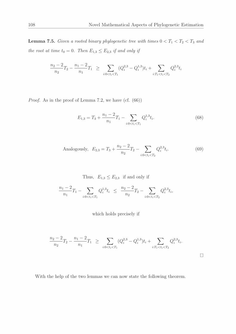
108 Novel Mathematical Aspects of Phylogenetic Estimation
Lemma 7.5. Given a rooted binary phylogenetic tree with times 0 < T1 < T2 < T3 and
the root at time t0 = 0. Then E1,3 ≤ E2,3 if and only if
n2 − 2
n2
T2 −n1 − 2
n1
T1 ≥∑
i:0<ti<T1
(Q2,3i − Q1,3
i )ti +∑
i:T1<ti<T2
Q2,3i ti
Proof. As in the proof of Lemma 7.2, we have (cf. (66))
E1,3 = T3 +n1 − 2
n1
T1 −∑
i:0<ti<T1
Q1,3i ti. (68)
Analogously, E2,3 = T3 +n2 − 2
n2
T2 −∑
i:0<ti<T2
Q2,3i ti. (69)
Thus, E1,3 ≤ E2,3 if and only if
n1 − 2
n1
T1 −∑
i:0<ti<T1
Q1,3i ti ≤ n2 − 2
n2
T2 −∑
i:0<ti<T2
Q2,3i ti,
which holds precisely if
n2 − 2
n2
T2 −n1 − 2
n1
T1 ≥∑
i:0<ti<T1
(Q2,3i − Q1,3
i )ti +∑
i:T1<ti<T2
Q2,3i ti.
With the help of the two lemmas we can now state the following theorem.
Expected Anomalies in the Fossil Record 109
Theorem 7.6. Given a rooted binary phylogenetic tree with times 0 < T1 < T2 < T3
and the root at time 0. Then, E1,3 ≤ min{E1,2, E2,3} if and only if the following two
conditions hold:
(i) T3 − T2 ≤∑
i:0<ti<T1
(Q1,3i − Q1,2
i )ti,
(ii) n2−2n2
T2 − n1−2n1
T1 ≥ ∑
i:0<ti<T1
(Q2,3i − Q1,3
i )ti +∑
i:T1<ti<T2
Q2,3i ti.
Proof. The Theorem follows directly from Lemmas 7.2 and 7.5.
The following example demonstrates the influence of times 0 < T1 < T2 < T3
according to the above theorem.
Example 7.7. Consider again Figure 7.1.
1. Assume t1 = 15, T1 = 100, t2 = 107, t3 = 109, T2 = 110, T3 = 130. Then, E1,2 =
137.33, E2,3 = 155.28 and E1,3 = 155.33. Hence, for this choice of times, we have
E1,3 > max{E1,2, E2,3}.
2. Consider the same times as in the previous case, but choose T2 = 129 instead
of T2 = 110. This means to move T2 further away from T1 and closer to T3.
This change is enough to give completely different expected values: E1,2 = 156.33,
E2,3 = 166.68 and E1,3 = 155.33. Hence, for this choice of times, we have E1,3 <
min{E1,2, E2,3}.
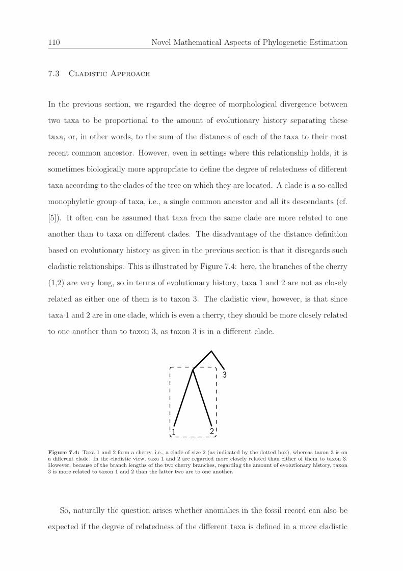
110 Novel Mathematical Aspects of Phylogenetic Estimation
7.3 Cladistic Approach
In the previous section, we regarded the degree of morphological divergence between
two taxa to be proportional to the amount of evolutionary history separating these
taxa, or, in other words, to the sum of the distances of each of the taxa to their most
recent common ancestor. However, even in settings where this relationship holds, it is
sometimes biologically more appropriate to define the degree of relatedness of different
taxa according to the clades of the tree on which they are located. A clade is a so-called
monophyletic group of taxa, i.e., a single common ancestor and all its descendants (cf.
[5]). It often can be assumed that taxa from the same clade are more related to one
another than to taxa on different clades. The disadvantage of the distance definition
based on evolutionary history as given in the previous section is that it disregards such
cladistic relationships. This is illustrated by Figure 7.4: here, the branches of the cherry
(1,2) are very long, so in terms of evolutionary history, taxa 1 and 2 are not as closely
related as either one of them is to taxon 3. The cladistic view, however, is that since
taxa 1 and 2 are in one clade, which is even a cherry, they should be more closely related
to one another than to taxon 3, as taxon 3 is in a different clade.
3
1 2
Figure 7.4: Taxa 1 and 2 form a cherry, i.e., a clade of size 2 (as indicated by the dotted box), whereas taxon 3 is ona different clade. In the cladistic view, taxa 1 and 2 are regarded more closely related than either of them to taxon 3.However, because of the branch lengths of the two cherry branches, regarding the amount of evolutionary history, taxon3 is more related to taxon 1 and 2 than the latter two are to one another.
So, naturally the question arises whether anomalies in the fossil record can also be
expected if the degree of relatedness of the different taxa is defined in a more cladistic
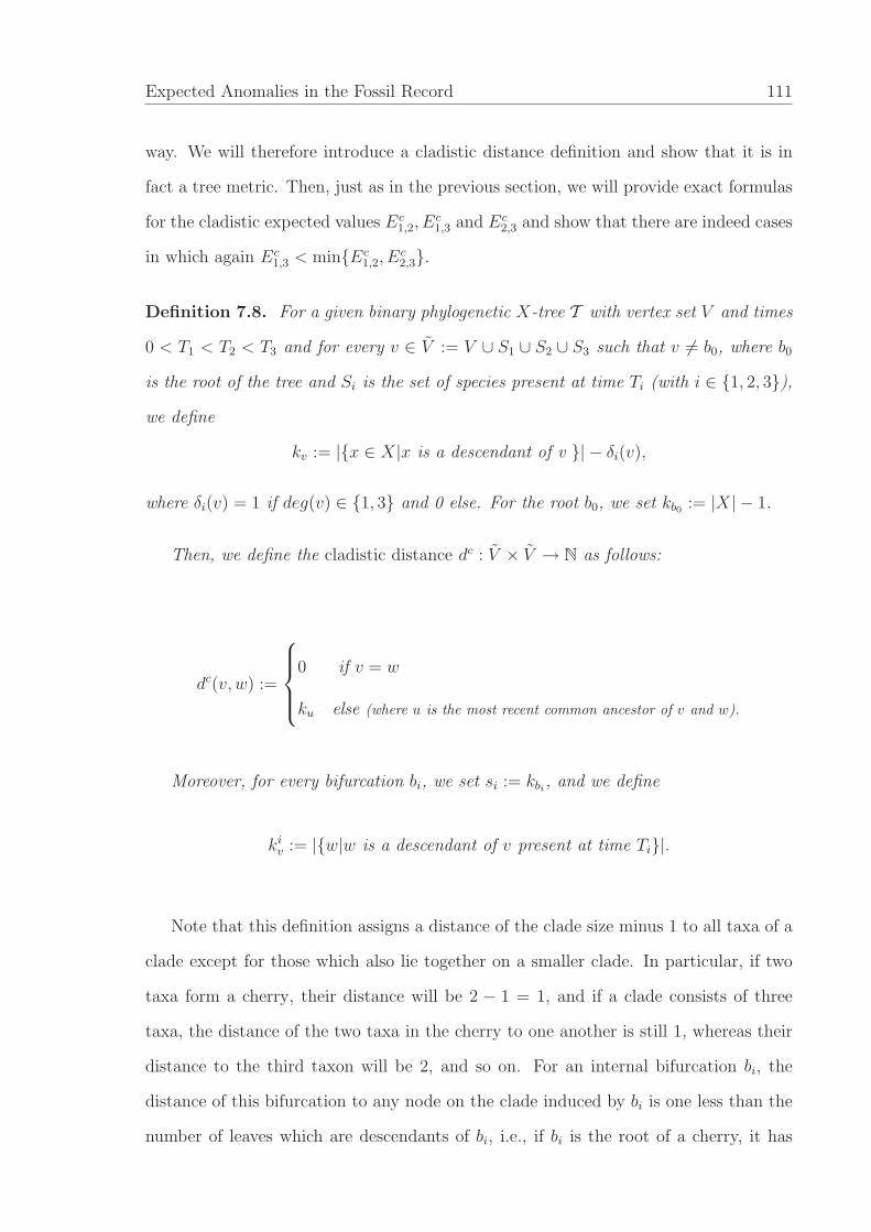
Expected Anomalies in the Fossil Record 111
way. We will therefore introduce a cladistic distance definition and show that it is in
fact a tree metric. Then, just as in the previous section, we will provide exact formulas
for the cladistic expected values Ec1,2, E
c1,3 and Ec
2,3 and show that there are indeed cases
in which again Ec1,3 < min{Ec
1,2, Ec2,3}.
Definition 7.8. For a given binary phylogenetic X-tree T with vertex set V and times
0 < T1 < T2 < T3 and for every v ∈ V := V ∪ S1 ∪ S2 ∪ S3 such that v 6= b0, where b0
is the root of the tree and Si is the set of species present at time Ti (with i ∈ {1, 2, 3}),
we define
kv := |{x ∈ X|x is a descendant of v }| − δi(v),
where δi(v) = 1 if deg(v) ∈ {1, 3} and 0 else. For the root b0, we set kb0 := |X| − 1.
Then, we define the cladistic distance dc : V × V → N as follows:
dc(v, w) :=
0 if v = w
ku else (where u is the most recent common ancestor of v and w).
Moreover, for every bifurcation bi, we set si := kbi, and we define
kiv := |{w|w is a descendant of v present at time Ti}|.
Note that this definition assigns a distance of the clade size minus 1 to all taxa of a
clade except for those which also lie together on a smaller clade. In particular, if two
taxa form a cherry, their distance will be 2 − 1 = 1, and if a clade consists of three
taxa, the distance of the two taxa in the cherry to one another is still 1, whereas their
distance to the third taxon will be 2, and so on. For an internal bifurcation bi, the
distance of this bifurcation to any node on the clade induced by bi is one less than the
number of leaves which are descendants of bi, i.e., if bi is the root of a cherry, it has
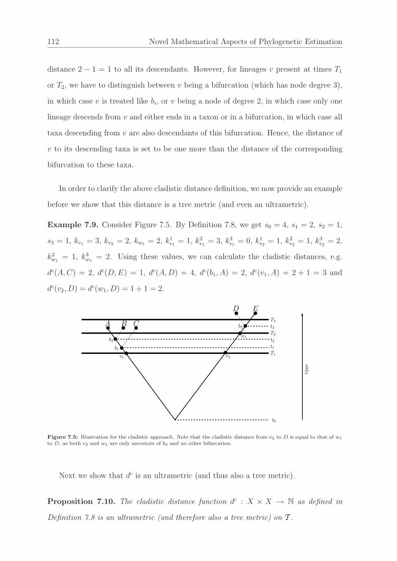
112 Novel Mathematical Aspects of Phylogenetic Estimation
distance 2 − 1 = 1 to all its descendants. However, for lineages v present at times T1
or T2, we have to distinguish between v being a bifurcation (which has node degree 3),
in which case v is treated like bi, or v being a node of degree 2, in which case only one
lineage descends from v and either ends in a taxon or in a bifurcation, in which case all
taxa descending from v are also descendants of this bifurcation. Hence, the distance of
v to its descending taxa is set to be one more than the distance of the corresponding
bifurcation to these taxa.
In order to clarify the above cladistic distance definition, we now provide an example
before we show that this distance is a tree metric (and even an ultrametric).
Example 7.9. Consider Figure 7.5. By Definition 7.8, we get s0 = 4, s1 = 2, s2 = 1,
s3 = 1, kv1 = 3, kv2 = 2, kw1 = 2, k1v1
= 1, k2v1
= 3, k3v1
= 0, k1v2
= 1, k2v2
= 1, k3v2
= 2,
k2w1
= 1, k3w1
= 2. Using these values, we can calculate the cladistic distances, e.g.
dc(A,C) = 2, dc(D,E) = 1, dc(A,D) = 4, dc(b1, A) = 2, dc(v1, A) = 2 + 1 = 3 and
dc(v2, D) = dc(w1, D) = 1 + 1 = 2.
C
tim
e
t0
v2
w1
T1
t1
t2
T2
t3
T3
b2
b1
v1
b3
D E
A B
Figure 7.5: Illustration for the cladistic approach. Note that the cladistic distance from v2 to D is equal to that of w1
to D, as both v2 and w1 are only ancestors of b3 and no other bifurcation.
Next we show that dc is an ultrametric (and thus also a tree metric).
Proposition 7.10. The cladistic distance function dc : X × X → N as defined in
Definition 7.8 is an ultrametric (and therefore also a tree metric) on T .
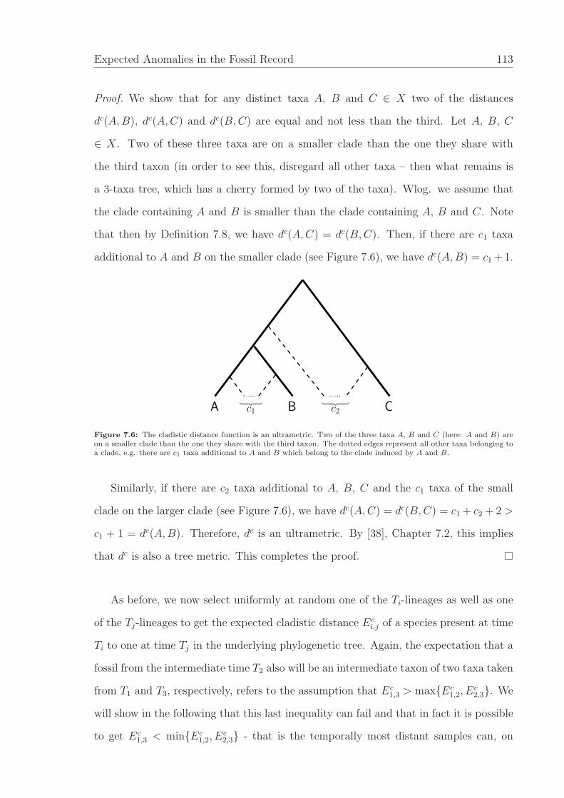
Expected Anomalies in the Fossil Record 113
Proof. We show that for any distinct taxa A, B and C ∈ X two of the distances
dc(A,B), dc(A,C) and dc(B,C) are equal and not less than the third. Let A, B, C
∈ X. Two of these three taxa are on a smaller clade than the one they share with
the third taxon (in order to see this, disregard all other taxa – then what remains is
a 3-taxa tree, which has a cherry formed by two of the taxa). Wlog. we assume that
the clade containing A and B is smaller than the clade containing A, B and C. Note
that then by Definition 7.8, we have dc(A,C) = dc(B,C). Then, if there are c1 taxa
additional to A and B on the smaller clade (see Figure 7.6), we have dc(A,B) = c1 +1.
A B C︸ ︷︷ ︸
c1︸ ︷︷ ︸
c2
Figure 7.6: The cladistic distance function is an ultrametric. Two of the three taxa A, B and C (here: A and B) areon a smaller clade than the one they share with the third taxon. The dotted edges represent all other taxa belonging toa clade, e.g. there are c1 taxa additional to A and B which belong to the clade induced by A and B.
Similarly, if there are c2 taxa additional to A, B, C and the c1 taxa of the small
clade on the larger clade (see Figure 7.6), we have dc(A,C) = dc(B,C) = c1 + c2 + 2 >
c1 + 1 = dc(A,B). Therefore, dc is an ultrametric. By [38], Chapter 7.2, this implies
that dc is also a tree metric. This completes the proof.
As before, we now select uniformly at random one of the Ti-lineages as well as one
of the Tj-lineages to get the expected cladistic distance Eci,j of a species present at time
Ti to one at time Tj in the underlying phylogenetic tree. Again, the expectation that a
fossil from the intermediate time T2 also will be an intermediate taxon of two taxa taken
from T1 and T3, respectively, refers to the assumption that Ec1,3 > max{Ec
1,2, Ec2,3}. We
will show in the following that this last inequality can fail and that in fact it is possible
to get Ec1,3 < min{Ec
1,2, Ec2,3} - that is the temporally most distant samples can, on
114 Novel Mathematical Aspects of Phylogenetic Estimation
average, be more similar than the temporally intermediate sample is to either of the
two, even in the cladistic setting.
Lemma 7.11. For a given binary phylogenetic X-tree and for times 0 < T1 < T2 < T3,
let dc be the cladistic distance function as defined in Definiton 7.8. Then, the expected
cladistic distance Ecj,l for j, l ∈ {1, 2, 3}, j < l, can be written as follows:
Ecj,l =
1
njnl
·
∑
i:ti<Tj
(P j,li · si) +
∑
v∈Sj
(klv · kv)
,
where Sj is the the set of species present at time Tj.
Proof. In the tree, there are njnl distinct paths connecting elements of Sj with elements
of Sl (as by definition, nj = |Sj|, nl = |Sl|). Thus, the expected value has to be divided
by this product. Moreover, as in the previous section the number of such ways employing
bi is denoted by P j,li , and for every bi (including the root b0), any path from Tj to Tl
along bi connects taxa which are on the clade induced by bi and not on any subclade.
Therefore, the cladistic distance between such species is by definition si. This explains
the first sum. The second sum is the sumation induced by direct ancestry: every species
present in time Tl has an ancestor v in Tj. The distance to this ancestor is by definition
kv, and there are by definition klv species present in time Tl which have v as an ancestor.
So altogether we have:
Ecj,l =
1
njnl
·
∑
i:ti<Tj
(P j,li · si)
︸ ︷︷ ︸distances
contributedby all bi’s
+∑
v∈Sj
(klv · kv)
︸ ︷︷ ︸distances
contributedby directancestry
.
This completes the proof.
Note that the expected values provided by Lemma 7.11 do not depend on the dis-
Expected Anomalies in the Fossil Record 115
tance between the times 0 < T1 < T2 < T3. Rather, they depend on the tree topology.
The times are only relevant in terms of the number of species present at each time.
This means that in this cladistic setting, there is no direct analog to Theorem 7.6.
More precisely, in order to find an example for which Ec1,3 < min{Ec
1,2, Ec2,3}, it is not
necessary to make a certain choice of values for T1, T2, T3. By making a suitable choice
of a tree topology, it is nevertheless possible to find examples for which fossils from T2
will on expectation be less related to fossils of times T1 and T3 than the latter two to
one another. We now provide such an example.
Example 7.12. Consider again the tree given in Figure 7.5 and the values calculated
in Example 7.9. The additional values needed to calculate the expected distances for
this example are n1 = 2, n2 = 4, n3 = 2, P 1,20 = 4, P 1,3
0 = 2, P 2,30 = 6, P 2,3
1 = 0,
P 2,32 = 0. Then, by Lemma 7.11, we get
Ec1,2 =
1
n1n2
·(∑
i:ti<T1
(P 1,2i · si) +
∑
v∈S1
(kkv · kv)
)
=1
2 · 4 · (4 · 4 + 3 · 3 + 1 · 2) =27
8
Ec2,3 =
1
n2n3
·(∑
i:ti<T2
(P 2,3i · si) +
∑
v∈S2
(kkv · kv)
)
=1
4 · 2 · (6 · 4 + 0 · 2 + 0 · 1 + 2 · 2) =28
8
Ec1,3 =
1
n1n3
·(∑
i:ti<T1
(P 1,3i · si) +
∑
v∈S1
(kkv · kv)
)
=1
2 · 2 · (2 · 4 + 0 · 3 + 2 · 2) =24
8
Therefore, Ec1,3 < min{Ec
1,2, Ec2,3}, and thus for the tree given in Figure 7.5, fossils
from times T1 and T3 can be expected to be more related to one another than to a
taxon from the intermediate time T2.
116 Novel Mathematical Aspects of Phylogenetic Estimation
7.4 Interpretation
The analysis of the fossil record provides an insight into the history of species and thus
into evolutionary processes. Stochastic models can provide a good approach to infer
patterns of diversification, and they form a useful link between molecular phylogenetics
and paleontology [29]. Such models would greatly benefit from incorporation of po-
tential fossil ancestors and other extinct data points to infer patterns of evolution. In
this chapter, we have applied a simple model-based phylogenetic approach to study the
expected degree of similarity between fossil taxa sampled at intermediate times.
‘Gaps’ in the fossil record are problematic [37] as they can be interpreted as ‘missing
links’. Therefore, numerous studies concerning the adequacy of the fossil record have
been conducted (see, for example, [8], [30], [45]), and it is frequently found that even
the available fossil record is still incompletely understood. This is particularly true
for ancestor-descendant relationships (see, for instance, [9], [15]). For example, Foote
[15] reported the probability that a preserved and recorded species has at least one
descendant species that is also preserved and recorded is on the order of 1% – 10%.
This number is much higher than the number of identified ancestor-descendant pairs.
Thus, it remains an important challenge to recognize such pairs [2]. This is also essential
with regard to ancestor-intermediate-descendant triplets, as it is possible that there are
in fact fewer ‘gaps’ than currently assumed, i.e., that intermediates are present but
not yet recognized. Such issues have an important bearing on any conclusions our
results might imply concerning the testing of hypotheses of continuous morphological
evolution, or concerning the shape of the underlying evolutionary tree based on the
non-existence of certain intermediates.
Another challenge is to investigate different phylogenetic models for describing the
expected degree of morphological separation between different fossil taxa sampled at
different times. Our findings of Chapter 7.2 strongly depend on the assumption that
morphological diversification is proportional to the distance in the underlying phyloge-
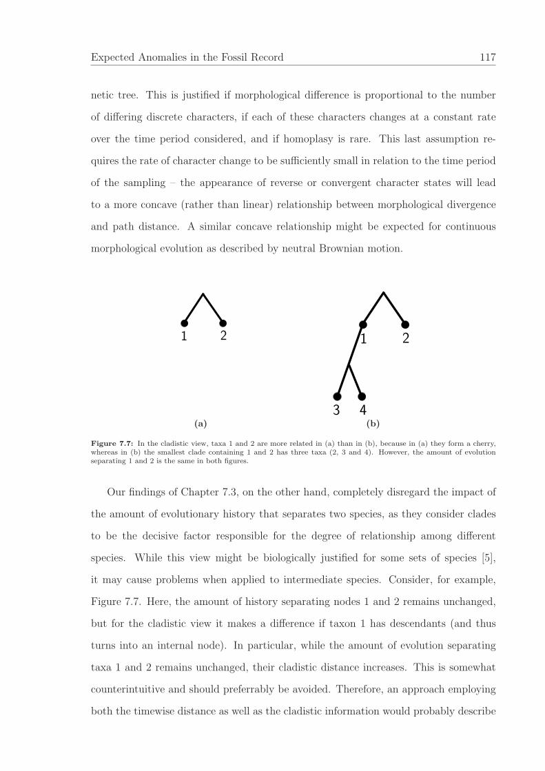
Expected Anomalies in the Fossil Record 117
netic tree. This is justified if morphological difference is proportional to the number
of differing discrete characters, if each of these characters changes at a constant rate
over the time period considered, and if homoplasy is rare. This last assumption re-
quires the rate of character change to be sufficiently small in relation to the time period
of the sampling – the appearance of reverse or convergent character states will lead
to a more concave (rather than linear) relationship between morphological divergence
and path distance. A similar concave relationship might be expected for continuous
morphological evolution as described by neutral Brownian motion.
21
(a)
21
3 4(b)
Figure 7.7: In the cladistic view, taxa 1 and 2 are more related in (a) than in (b), because in (a) they form a cherry,whereas in (b) the smallest clade containing 1 and 2 has three taxa (2, 3 and 4). However, the amount of evolutionseparating 1 and 2 is the same in both figures.
Our findings of Chapter 7.3, on the other hand, completely disregard the impact of
the amount of evolutionary history that separates two species, as they consider clades
to be the decisive factor responsible for the degree of relationship among different
species. While this view might be biologically justified for some sets of species [5],
it may cause problems when applied to intermediate species. Consider, for example,
Figure 7.7. Here, the amount of history separating nodes 1 and 2 remains unchanged,
but for the cladistic view it makes a difference if taxon 1 has descendants (and thus
turns into an internal node). In particular, while the amount of evolution separating
taxa 1 and 2 remains unchanged, their cladistic distance increases. This is somewhat
counterintuitive and should preferrably be avoided. Therefore, an approach employing
both the timewise distance as well as the cladistic information would probably describe

118 Novel Mathematical Aspects of Phylogenetic Estimation
the relationships amongst different species best. But since for both the pure cladistic
as well as the pure history-based approach it was possible to construct examples in
which the expected degree of relatedness of fossils from two distant times is less than to
fossils of an intermediate time, we conjecture that even in a model that combines both
approaches, such cases may exist. But this does not necessarily have to be bad news:
in fact, gaps caused by a scenario as described in Chapter 7.2 may even give some faint
hints on the shape and size of the underlying phylogenetic tree in the light of Theorem
7.6.
Chapter 8
Conclusion and Outlook
I am still confused. But on a higher level.
Enrico Fermi
The main purpose of this thesis was to present some very surprising properties
of the most important tree inference techniques. Many of these ‘surprises’, such as
presented in Chapters 4 and 5, deal with scenarios in which different methods lead to
different trees. At first glance, such scenarios may seem more curious in a biological
sense than in a mathematical one – as, from the mathematical point of view, one
might wonder right away why different methods should lead to the same result. In this
respect, examples in which Maximum Parsimony gives a tree which differs from the one
induced by distance-based methods or by Maximum Likelihood might not seem too
curious at all. Therefore, in this thesis we presented not only examples for such cases,
but additionally the mathematical ideas which can be used to construct such examples
for any number of taxa. Moreover, Chapter 5 shows that the likelihood support for a
tree which is not most parsimonious can be made arbitrarily large under only slight
modifications of the ‘no common mechanism’ Nr-model, even though without these
modifications MP and ML are equivalent. Chapter 4 gives precise instructions on how
to construct sequences which are homoplasy-free (and thus MP-wise ‘best possible’)
on one tree and treelike (and thus distance-wise ‘best possible’) on a different tree
– where both trees can be freely chosen. In this sense, our findings are indeed also
mathematically surprising, because they show that arbitrarily many examples can be
constructed and that these examples can make the gap between different methods
arbitrarily large.
119
120 Novel Mathematical Aspects of Phylogenetic Estimation
On the other hand, as mentioned above, some of the results presented in this thesis
are even more surprising from a biological point of view. As demonstrated in Chapter
5, the often cited and well-known equivalence of MP and ML under the ‘no common
mechanism’ Nr-model fails under certain additional assumptions of biological relevance
– such as a molecular clock or bounded (and thus small) substitution probabilities.
In the latter case, MP has traditionally been believed to be justified in the sense of
agreement with ML (for a further discussion of this issue, the reader is referred to [12],
pp. 100 ff.). Moreover, in Chapter 3 we showed that the Fitch algorithm sometimes
provides a better estimation of the ancestral root state when some taxa are ignored
– and that these taxa may even be arbitrarily close to the root. This is biologically
counterintuitive as on short branches the probability of the conservation of the root
state is relatively high, which is why it seems logical that MP should take them into
account. Our example shows that, surprisingly, this is not in general true – in particular,
if the rest of the tree fulfills certain properties, e.g. concerning balance, this part of
the tree alone can provide a better estimate of the root state than when combined with
other taxa.
Results that show how certain methods can disagree when inferring trees are not
necessarily ‘bad news’ for phylogeneticists. They rather contribute to the general under-
standing of these methods and underline the importance of choosing the ‘right’ method
and model for the analysis of particular data sets. In the same sense, Chapter 6 can be
regarded as useful, as the sequence length bounds provided in this chapter may indicate
that certain sequences simply are not long enough for a reliable tree reconstruction.
Chapter 7 is somewhat unrelated to the other chapters as it does not analyze existing
methods or models but rather introduces a novel way to explain the degree of relatedness
of different fossils using a simple stochastic model. Moreover, it is maybe the only
chapter in this thesis whose results can be regarded as ‘good news’ already at first glance:
here, we do not highlight disagreements of different methods, we rather explain why the
perceived ‘disagreement’ of the patchy fossil record with the assumption of a continuous
Conclusion and Outlook 121
evolutionary process can in some cases (at least partially) be resolved. We show that
some tree topologies and certain choices of times have the curious property that fossils
from an intermediate time can be expected not to be morphologically intermediate.
Additionally, we have shown that this property does not necessarily disappear when a
more cladistic view is assumed. While the models used in this chapter are very simple,
we are convinced that similar results can be achieved for more complex models, too –
in particular if these combine the history-based and the cladistic view.
Solving mathematical problems may in a way be a thankless job: along with the sat-
isfaction of having answered one question often comes the comprehension that ten more
questions arise from the solution. For instance, finding a way to construct sequences
of binary and ternary characters whose perfect phylogeny and perfect distance-based
tree differ, was satisfactory in the sense that this result is best possible concerning the
number of character states (as binary sequences are already known to be insufficient for
this purpose). Similarly, finding a way of causing discrepancies between MP and ML for
certain modifications of the Nr-model with no common mechanism was positive. And
finally, the realization that these seemingly unrelated problems can be approached using
similar techniques, and that even some sequences for which MP and and the derived
Hamming distances disagree can be used to find an upper bound on the substitution
probabilities such that MP and ML will also disagree for the same sequences, was as-
tonishing. But, naturally, this cognition leads to many more questions: is there always
an upper bound on the substitution probabilities such that for treelike sequences, ML
will agree with the tree on which the distances are additive? What is the relationship
of ML and distance-based methods like Neighbor-Joining in general? Are there binary
sequences which lead, with an appropriate choice of an upper bound for the substitu-
tion probabilities or under the restriction of a molecular clock, to conflicting choices of
MP and ML? These questions are beyond the scope of this thesis, but they certainly
provide grounds for future research.
While we are confident that this thesis throws light on some surprising and curious

122 Novel Mathematical Aspects of Phylogenetic Estimation
aspects of phylogenetics, we also appreciate that even 35 years after Fitch’s parsimony
algorithm was first introduced and 30 years after the discovery of the Felsenstein zone,
there are still properties even of the most frequently used and discussed tree inference
methods which are unknown – which is why all these methods are still worth further
investigation.
Appendix
Here we present in detail the analysis of the likelihood of the character f1 := aabb on
tree T1 := 12|34 under the N3-model (with state set {A,B,C}) with the help of the
computer algebra system MAXIMA.
Notation: The pending edges of T1 are denoted by ei, for leaves i = 1, . . . , 4, with
substitution probabilities pi, respectively. We evaluate the likelihood by Felsenstein’s
postorder traversal [11] rooting the tree at leaf 1 (where the likelihood does not depend
on the root position). The interior edge is denoted by e5 = (v, w), where w is the
vertex at which the edges e1 and e2 are pending, and v is the vertex at which e3 and
e4 are pending. The substitution probability for the interior edge e5 is denoted by p5.
Moreover, we denote by Av, Bv and Cv the likelihood of character f1 restricted to the
vertices below v (that is, vertices 3 and 4) conditional on v being in state A, B or C,
respectively. Similarly, Aw is the likelihood of the character restricted to 2,3,4 (which
are the vertices below w) conditional on w being in state A, and so on. We denote by
u the upper bound on the substitution probabilities. By Corollary 5.4 we know that
the likelihood is maximized at a point where all substitution probabilities are either 0
or u, so these are the only cases for which we have to calculate the likelihood values.
123
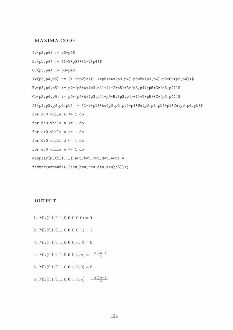
MAXIMA CODE
Av(p3,p4) := p3*p4$
Bv(p3,p4) := (1-2*p3)*(1-2*p4)$
Cv(p3,p4) := p3*p4$
Aw(p3,p4,p5) := (1-2*p2)*((1-2*p5)*Av(p3,p4)+p5*Bv(p3,p4)+p5*Cv(p3,p4))$
Bw(p3,p4,p5) := p2*(p5*Av(p3,p4)+(1-2*p5)*Bv(p3,p4)+p5*Cv(p3,p4))$
Cw(p3,p4,p5) := p2*(p5*Av(p3,p4)+p5*Bv(p3,p4)+(1-2*p5)*Cv(p3,p4))$
A1(p1,p2,p3,p4,p5) := (1-2*p1)*Au(p3,p4,p5)+p1*Bu(p3,p4,p5)+p1*Cu(p3,p4,p5)$
for a:0 while a <= 1 do
for b:0 while b <= 1 do
for c:0 while c <= 1 do
for d:0 while d <= 1 do
for e:0 while e <= 1 do
display(ML(f_1,T_1,a*u,b*u,c*u,d*u,e*u) =
factor(expand(A1(a*u,b*u,c*u,d*u,e*u)/3)));
OUTPUT
1. ML (f 1, T 1, 0, 0, 0, 0, 0) = 0
2. ML (f 1, T 1, 0, 0, 0, 0, u) = u3
3. ML (f 1, T 1, 0, 0, 0, u, 0) = 0
4. ML (f 1, T 1, 0, 0, 0, u, u) = −u (2 u−1)3
5. ML (f 1, T 1, 0, 0, u, 0, 0) = 0
6. ML (f 1, T 1, 0, 0, u, 0, u) = −u (2 u−1)3
124
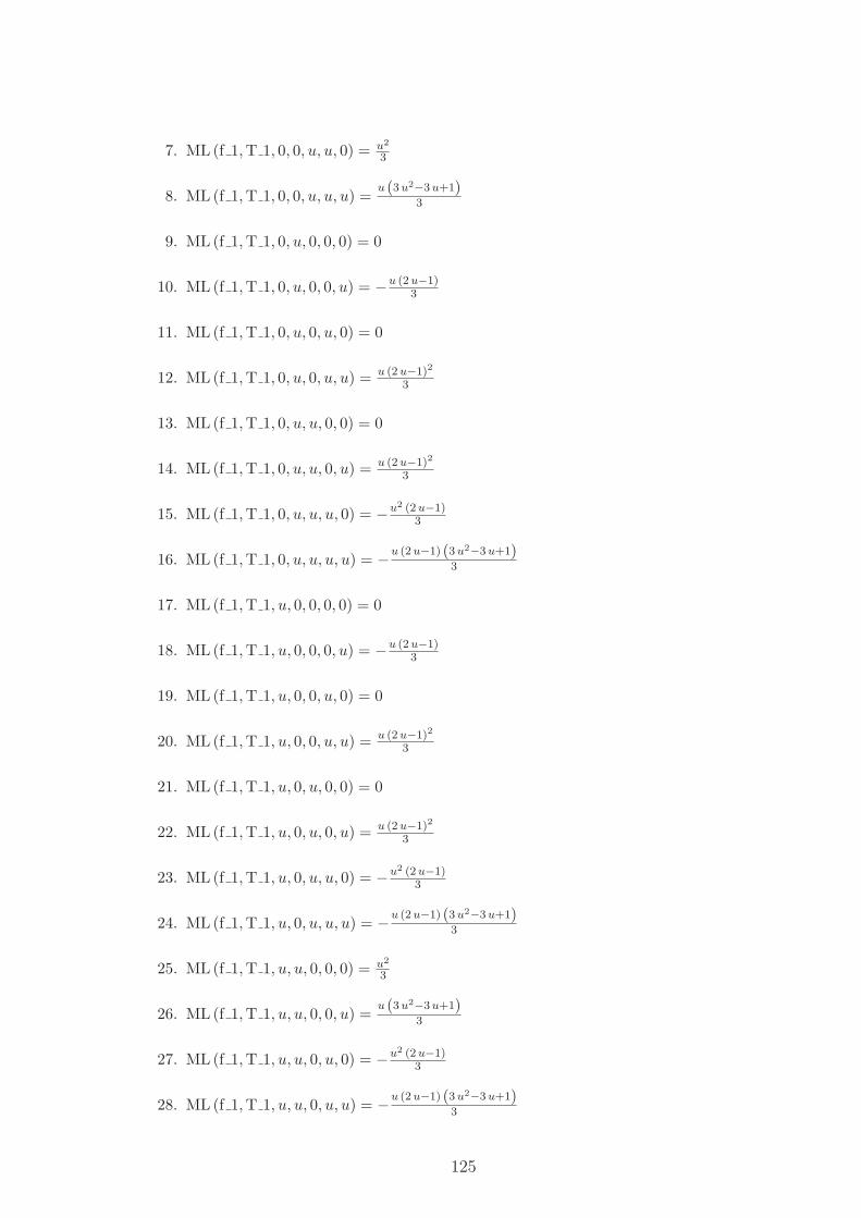
7. ML (f 1, T 1, 0, 0, u, u, 0) = u2
3
8. ML (f 1, T 1, 0, 0, u, u, u) =u (3 u2−3 u+1)
3
9. ML (f 1, T 1, 0, u, 0, 0, 0) = 0
10. ML (f 1, T 1, 0, u, 0, 0, u) = −u (2 u−1)3
11. ML (f 1, T 1, 0, u, 0, u, 0) = 0
12. ML (f 1, T 1, 0, u, 0, u, u) = u (2 u−1)2
3
13. ML (f 1, T 1, 0, u, u, 0, 0) = 0
14. ML (f 1, T 1, 0, u, u, 0, u) = u (2 u−1)2
3
15. ML (f 1, T 1, 0, u, u, u, 0) = −u2 (2 u−1)3
16. ML (f 1, T 1, 0, u, u, u, u) = −u (2 u−1) (3 u2−3 u+1)3
17. ML (f 1, T 1, u, 0, 0, 0, 0) = 0
18. ML (f 1, T 1, u, 0, 0, 0, u) = −u (2 u−1)3
19. ML (f 1, T 1, u, 0, 0, u, 0) = 0
20. ML (f 1, T 1, u, 0, 0, u, u) = u (2 u−1)2
3
21. ML (f 1, T 1, u, 0, u, 0, 0) = 0
22. ML (f 1, T 1, u, 0, u, 0, u) = u (2 u−1)2
3
23. ML (f 1, T 1, u, 0, u, u, 0) = −u2 (2 u−1)3
24. ML (f 1, T 1, u, 0, u, u, u) = −u (2 u−1) (3 u2−3 u+1)3
25. ML (f 1, T 1, u, u, 0, 0, 0) = u2
3
26. ML (f 1, T 1, u, u, 0, 0, u) =u (3 u2−3 u+1)
3
27. ML (f 1, T 1, u, u, 0, u, 0) = −u2 (2 u−1)3
28. ML (f 1, T 1, u, u, 0, u, u) = −u (2 u−1) (3 u2−3 u+1)3
125
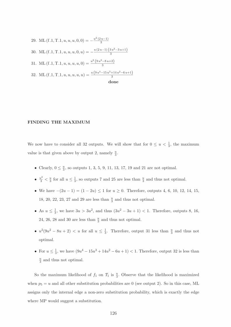
29. ML (f 1, T 1, u, u, u, 0, 0) = −u2 (2 u−1)3
30. ML (f 1, T 1, u, u, u, 0, u) = −u (2 u−1) (3 u2−3 u+1)3
31. ML (f 1, T 1, u, u, u, u, 0) =u2 (9 u2−8 u+2)
3
32. ML (f 1, T 1, u, u, u, u, u) =u (9 u4−15 u3+14 u2−6 u+1)
3
done
FINDING THE MAXIMUM
We now have to consider all 32 outputs. We will show that for 0 ≤ u < 13 , the maximum
value is that given above by output 2, namely u3 .
• Clearly, 0 ≤ u3 , so outputs 1, 3, 5, 9, 11, 13, 17, 19 and 21 are not optimal.
• u2
3 < u3 for all u ≤ 1
3 , so outputs 7 and 25 are less than u3 and thus not optimal.
• We have −(2u − 1) = (1 − 2u) ≤ 1 for u ≥ 0. Therefore, outputs 4, 6, 10, 12, 14, 15,
18, 20, 22, 23, 27 and 29 are less than u3 and thus not optimal.
• As u ≤ 13 , we have 3u > 3u2, and thus (3u2 − 3u + 1) < 1. Therefore, outputs 8, 16,
24, 26, 28 and 30 are less than u3 and thus not optimal.
• u2(9u2 − 8u + 2) < u for all u ≤ 13 . Therefore, output 31 less than u
3 and thus not
optimal.
• For u ≤ 13 , we have (9u4 − 15u3 + 14u2 − 6u + 1) < 1. Therefore, output 32 is less than
u3 and thus not optimal.
So the maximum likelihood of f1 on T1 is u3 . Observe that the likelihood is maximized
when p5 = u and all other substitution probabilities are 0 (see output 2). So in this case, ML
assigns only the internal edge a non-zero substitution probability, which is exactly the edge
where MP would suggest a substitution.
126
List of Symbols
Symbol Meaning
AA ambiguous reconstruction accuracy of Maximum ParsimonyA|B X-splitbi bifurcation at a time tibp base pairsc character stateC set of character statesd(x, y) time-based distance between two taxa x and ydc(x, y) cladistic distance between two taxa x and ydS(x, y) Hamming distance between taxa x and y induced by SE(T ) edge set of a tree TEi,j expected time-based distance of species of time Ti to species of time Tj
Eci,j expected cladistic distance of species of time Ti to species of time Tj
f characteridS
(σ) isolation index of an X-split σ for a sequence Sg extension of a characterlT (f) parsimony score of a character f on a tree TlT (g) parsimony score of an extension g of a character on a tree Tpe,i substitution probability of a character fi on an edge e
P j,ki number of paths from time Tj to time Tk along node bi
r number of character statesRA reconstruction accuracy of Maximum ParsimonyS character sequenceσ X-splitΣ(X) set of X-splitsΣ∗(X) set of non-trivial X-splitsT phylogenetic treeT , t fixed timeTY restriction of an X-tree T to a subset Y ⊆ Xu upper bound on the substitution probabilityUA unambiguous reconstruction accuracy of Maximum ParsimonyV (T ) vertex set of a tree TX set of leaves of a tree Twlog. without loss of generality
127

128 Novel Mathematical Aspects of Phylogenetic Estimation
List of Figures
1.1 The only sketch of a phylogenetic tree in Darwin’s ‘The Origin of Species’ . . . 1
3.1 A tree on which MP is more accurate when applied to Y ⊂ X. . . . . . . . . . 18
3.2 Illustration for Theorem 3.3 . . . . . . . . . . . . . . . . . . . . . . . . . . . . . 20
4.1 Illustration of Equation 5 . . . . . . . . . . . . . . . . . . . . . . . . . . . . . . 28
4.2 Example of a misleading sequence . . . . . . . . . . . . . . . . . . . . . . . . . 32
4.3 Trees derived from the sequence given in Figure 4.2 . . . . . . . . . . . . . . . . 33
4.4 Huson-Steel sequence derived by the trees given in Figure 4.3 . . . . . . . . . . 37
4.5 Illustration of the three unrooted trees on four taxa. . . . . . . . . . . . . . . . 39
4.6 Illustration of the perfect phylogeny versus the perfect distance-tree . . . . . . 44
4.7 DNA alignment of human, chicken, mouse and rat . . . . . . . . . . . . . . . . 45
4.8 Shortened version of the alignment given in Figure 4.7 . . . . . . . . . . . . . . 46
4.9 The perfect phylogeny and the distance-based tree for the alignment of Figure
4.8. . . . . . . . . . . . . . . . . . . . . . . . . . . . . . . . . . . . . . . . . . . . 47
5.1 Illustration of labelled and unlabelled blocks . . . . . . . . . . . . . . . . . . . . 56
5.2 The characters f1 and f2 both correspond to a split on an interior edge of T1
or T2, respectively. But, as highlighted by the circled leaves, the assignment of
f1 on T2 differs from the assignment of f2 to T1. . . . . . . . . . . . . . . . . . . 59
5.3 Tree T3 is both an MP- and an ML-tree for sequence S . . . . . . . . . . . . . . 61
129
130 Novel Mathematical Aspects of Phylogenetic Estimation
5.4 Illustration of the unique MP tree versus the perfect distance-tree . . . . . . . 61
5.5 Clocklike example for which the MP- and ML-trees differ . . . . . . . . . . . . 68
5.6 Binary clocklike example for an MP-tree which is not an ML-tree . . . . . . . . 71
6.1 The 4-taxa setting with short internal edge and long pending edges . . . . . . . 79
6.2 The density of the standard normal distribution . . . . . . . . . . . . . . . . . . 85
7.1 Illustration of the fossil setting . . . . . . . . . . . . . . . . . . . . . . . . . . . 102
7.2 One-branch example for the approach using evolutionary history . . . . . . . . 103
7.3 Two-branch example for the approach using evolutionary history . . . . . . . . 103
7.4 Illustration of the cladistic approach . . . . . . . . . . . . . . . . . . . . . . . . 110
7.5 Example for the cladistic approach . . . . . . . . . . . . . . . . . . . . . . . . . 112
7.6 The cladistic distance function is an ultrametric. . . . . . . . . . . . . . . . . . 113
7.7 The problem of internal nodes in the cladistic approach. . . . . . . . . . . . . . 117

List of Tables
1 List of publications resulting from this thesis . . . . . . . . . . . . . . . . . . . 3
2 Overview of the values needed for the Huson-Steel approach . . . . . . . . . . . 36
3 15 different patterns on 4 taxa . . . . . . . . . . . . . . . . . . . . . . . . . . . 38
4 Summary of the information induced by Figure 4.8 . . . . . . . . . . . . . . . . 46
5 Results of the whole genome alignment . . . . . . . . . . . . . . . . . . . . . . . 48
131

132 Novel Mathematical Aspects of Phylogenetic Estimation
Index
4-point condition, see Four-point condition
additive distances, 11, 26, 31, 32, 36, 39, 40,
47–49
alignment, 45–47
ambigous MP reconstruction accuracy, 14, 15
ancestral root state reconstruction, 13, 22, 23
Azuma’s inequality, 90–92
bifurcation, 101, 102, 104, 107, 111, 112
block, 56
branch, 102, 104
Brownian motion, 117
Cavender-Farris-Neyman model, 6
Central Limit approximation, 79, 88
Central Limit Theorem, 88, 92
character, 5
extension, 6, 53, 55, 57, 58, 65
informative, 5, 8, 8, 39, 44–46
non-informative, 5, 8, 26, 32, 41, 50, 75
state, 5
uninformative, see non-informative
characterization of misleading sequences, 38,
41
cherry, 110, 111
clade, 110, 111, 114, 117
clocklike, see molecular clock
CLT, see Central Limit Theorem
common ancestor, 99, 103, 110
convex, 8, see homoplasy-free
density
standard normal distribution, 85
distance
cladistic, 100, 111–113
corrected, 10, 49
Hamming, 10, 26, 27, 39, 41, 64, 75
Hellinger, 79, 81, 83, 84
misleading, 27
mismatch, see Hamming distance
morphological, 104
treelike, 10, 36, 46, 48, 64, 100
distance-based methods, 9
DNA sequences, 48, 77
evolutionary history, 103, 110
extension, see character extension
extinction, 101, 107
Felsenstein zone, 51
Fitch parsimony, 8, 13, 14, 22
fossil, 23, 116, 118
fossil record, 99, 100, 110, 116
fossilization, 99
Four-point condition, 10, 39, 40
133
134 Novel Mathematical Aspects of Phylogenetic Estimation
galGal12, 45
gap, 99, 100, 116, 118
Hadamard representation, 82
height (of a tree), 71, 103
Hellinger distance, see distance
hg18, 45
hidden changes, 10, 49
homoplasy, 97, 117
homoplasy-free, 8, 31, 36, 40, 44–47, 49, 92,
93
human genome, 45
i.i.d., 7, 80, 81, 85, 86, 88, 92, 95
incongruent trees, 47, 49
infinite state model, 79
intermediate, 99, 114, 116–118
Jukes-Cantor model, 6
Markov process, 7, 77, 79, 80, 92, 93, 95–98
maximal subtree, 56
Maximum Likelihood (ML), 9, 50–52, 58, 65,
66
Maximum Likelihood tree (ML-tree), 9, 9, 45,
55, 67, 70, 75
Maximum Parsimony (MP), 7, 13–16, 22, 51,
58, 78, 80, 84, 86, 89–91, 93
Maximum Parsimony tree (MP-tree), 8, 25,
41, 67, 68, 70, 75
metazoa, 78
misleading distances, 25, 31–33, 36, 38, 40, 45,
48, 49
misleading sequence, 27, 64
misleading taxon, 16, 19
mismatch distance, 32
missing link, 116
mm8, 45
molecular clock, 11, 13, 19, 20, 22, 23, 31–34,
38, 46, 67, 74
monophyletic group, 110
morphological characteristic, 100
morphological divergence, 100, 103, 110
morphological diversification, 116
morphological diversity, 103
most parsimonious extension, 8
MP reconstruction probability, see reconstruc-
tion probability
MP-score, see parsimony score
multilinearity, 51, 54, 55
Nr-model, 6, 9, 14, 19, 52, 57, 58, 65, 66, 74,
76, 80, 85, 88, 97
Neighbor-Joining, 9
network, 48
no common mechanism, 7, 9, 51, 52, 57, 58,
65, 66, 74, 76
normal distribution, 86
nucleotide substitution, 25
paleontology, 116
parsimony score, 8, 49, 55, 65, 71, 87
parsmimony score, 52
partition, 5, 31, 46
perfect phylogeny, 8, 32, 36, 48, 64, 75
INDEX 135
photosynthesis, 78
phylogenetic X-tree, 5
Random Cluster Model, 7
random cluster model, 92, 92, 93, 97
rate matrix, 95
reconstruction accuracy, 8, 15, 16, 18, 20, 22,
23
reconstruction probability, 84, 85, 87–89, 92,
93, 95
rheMac2, 47
rn4, 45
root, 14, 65, 73, 99, 101, 105
of a molecular clock, 11
rooted phylogenetic X-tree, 5
rooted subtree, 14
sequence length, 26, 34–36, 41, 43
speciation event, 78
split, 5, 32
split metric, 11, 26, 27, 29, 30
standard normal distribution, 85, 89
star tree, 30, 32, 73
state, see character state
substitution, 6, 55, 79
substitution probability, 9, 16, 52, 53, 55–57,
65, 66, 75, 89, 92
bounded, 58
substitution rate, 77
symmetric r-state model, see Nr-model
tree metric, 10, 40
triangle inequality, 40, 97
UCSC Genome Browser, 45
ultrametric, see molecular clock
unambigous MP reconstruction accuracy, 14,
15
unresolved tree, 30
weakly misleading sequences, 47
whole genome, 47
window size, 47
X-split
non-trivial, 5, 31
trivial, 5

136 Novel Mathematical Aspects of Phylogenetic Estimation
Publications Resulting
from this Thesis
[BF08] H.-J. Bandelt and M. Fischer. Perfectly misleading distances from ternary characters.
Syst. Biol., 57(4):540–543, 2008.
[FS08] M. Fischer and M. Steel. Expected anomalies in the fossil record. Evol. Bioinf. Onl.,
4:61–67, 2008.
[FS09] M. Fischer and M. Steel. Sequence length bounds for resolving a deep phylogenetic
divergence. J. Theo. Biol., 256:247–252, 2009.
[FT09a] M. Fischer and B. Thatte. Maximum parsimony on subsets of taxa. Submitted to J.
Theo. Biol., 2009.
[FT09b] M. Fischer and B. Thatte. Revisiting an equivalence between maximum parsimony
and maximum likelihood methods in phylogenetics. Submitted to Bull. Math. Biol.,
2009.
137

138 Novel Mathematical Aspects of Phylogenetic Estimation
Bibliography
[1] Alon, N., and Spencer, J. The probabilistic method. John Wiley and Sons, New
York, 2000.
[2] Alroy, J. Continuous track analysis: a new phylogenetic and biogeographic method.
Syst. Biol. 44 (1995), 152 – 178.
[3] Atteson, K. The performance of neighbor-joining methods of phylogenetic reconstruc-
tion. Algorithmica 25 (1999), 251 – 278.
[4] Bandelt, H.-J., and Dress, A. Reconstructing the shape of a tree from observed
dissimilarity data. Adv. Appl. Math. 7 (1986), 309–343.
[5] Benton, M., and Harper, D. Basic paleontology. Prentice Hall, 1997.
[6] Churchill, G., von Haeseler, A., and Navidi, W. Sample size for a phylogenetic
inference. Mol. Biol. Evol. 9(4) (1992), 753–769.
[7] Darwin, C. On the origin of species by means of natural selection, or the preservation
of favoured races in the struggle for life. John Murray, London, 1859.
[8] Durham, J. The incompleteness of our knowledge of the fossil record. J. Paleont. 41
(1967), 559 – 565.
[9] Engelmann, G., and Wiley, E. The place of ancestor-descendant relationships in
phylogeny reconstruction. Syst. Zool. 26 (1977), 1 – 11.
[10] Felsenstein, J. Cases in which parsimony or compatibility will be positively misleading.
Syst. Zool. 27 (1978), 401–410.
[11] Felsenstein, J. Evolutionary trees from dna sequences: a maximum likelihood ap-
proach. J. Mol. Evol. 17 (1981), 368–376.
139
140 Novel Mathematical Aspects of Phylogenetic Estimation
[12] Felsenstein, J. Inferring phylogenies. Sinauer Associates, Massachusetts, 2004.
[13] Fischl, W. Distances that perfectly mislead: a practical approach. Project report,
2007.
[14] Fitch, W. Toward defining the course of evolution: minimum change for a specific tree
topology. Syst. Zool. 20(4) (1971), 406–416.
[15] Foote, M. On the probability of ancestors in the fossil record. Paleobiol. 22(2) (1996),
141 – 151.
[16] Hendy, M. The relationship between simple evolutionary tree models and observable
sequence data. Syst. Zool. 38 (1989), 310–321.
[17] Hendy, M., and Penny, D. A framework for the qualitative study of evolutionary
trees. Syst. Zool. 38 (1989), 297–309.
[18] Huber, K., Moulton, V., and Steel, M. Four characters suffice to convexly define
a phylogenetic tree. SIAM J. discr. Math. 18(4) (2005), 835–843.
[19] Huson, D., and Steel, M. Distances that perfectly mislead. Syst. Biol. 53(2) (2004),
327 – 332.
[20] Jukes, T., and Cantor, C. Evolution of protein molecules. In “Mammalian Protein
Metabolism”, New York Academic Press (1969), 21–132.
[21] Lecointre, G., Philippe, H., van Le, H., and Le Guyader, H. How many nu-
cleotides are required to resolve a phylogenetic problem? the use of a new statistical
method applicable to available sequences. Mol. Phyl. Evol. 3(4) (1994), 292–309.
[22] Li, G., Steel, M., and Zhang, L. More taxa are not necessarily better for the
reconstruction of ancestral character state. Syst. Biol. 57(4) (2008), 647 – 653.
[23] Lockhart, P., Novis, P., Milligan, B., Riden, J., Rambaut, A., and T., L.
Heterotachy and tree building: a case study with plastids and eubacteria. Mol. Biol.
Evol. 23(1) (2006), 40–45.
BIBLIOGRAPHY 141
[24] Marshall, C. Confidence intervals on stratigraphic ranges. Paleobiol. 16(1) (1990), 1
– 10.
[25] Marshall, C. The fossil record and estimating divergence times between lineages:
maximum divergence times and the importance of reliable phylogenies. J. Mol. Evol. 30
(1990), 400 – 408.
[26] McDiarmid, C. On the method of bounded differences. Surveys in Combinatorics, J.
Siemons ed., London Mathematical Society Lecture Note Series 141, Cambridge Univer-
sity Press (1989), 148–188.
[27] Mossel, E., and Steel, M. A phase transition for a random cluster model on phylo-
genetic trees. Math. Biosci. 187 (2004), 189–203.
[28] Mossel, E., and Steel, M. How much can evolved characters tell us about the
tree that generated them? In: Olivier Gascuel (ed.), Mathematics of Evolution and
Phylogeny, Oxford University Press (2005), 384–412.
[29] Nee, S. Extinct meets extant: simple models in paleontology and molecular phyloge-
netics. Paleobiol. 30(2) (2004), 172 – 178.
[30] Newell, N. Adequacy of the fossil record. J. Paleont. 33 (1959), 488 – 499.
[31] Neyman, J. Molecular studies of evolution: A source of novel statistical problems.
In “Statistical Decision Theory and Related Topics”, New York Academic Press (1971),
1–27.
[32] Philippe, H., Delsuc, F., Brinkmann, H., and Lartillot, N. Phylogenomics.
Annu. Rev. Ecol. Evol. Syst. 36 (2005), 541–562.
[33] Rokas, A., and Carrol, S. Bushes in the tree of life. PLoS Biology 4(11) (2006),
e352.
[34] Rozanov, Y. Probability theory: a concise course. Dover Publications, New York, 1969.
[35] Saitou, N., and Nei, M. The number of nucleotides required to determine the branch-
ing order of three species, with special reference to the human-chimpanzee-gorilla diver-
gence. J. Mol. Evol. 24 (1986), 189–204.
142 Novel Mathematical Aspects of Phylogenetic Estimation
[36] Salisbury, B., and Kim, J. Ancestral state estimation and taxon sampling density.
Syst. Biol. 50(4) (2001), 557–564.
[37] Schoch, R. Gaps in the fossil record. Nature 299 (1982), 490.
[38] Semple, C., and Steel, M. Phylogenetics. Oxford University Press, 2003.
[39] Sober, E. Evidence and Evolution: the logic behind the science. Cambridge Unversity
Press, 2008.
[40] Steel, M., and Charleston, M. Five surprising properties of parsimoniously colored
trees. Bulletin of Mathematical Biology 57(2) (1995), 367–375.
[41] Steel, M., and Szekely, L. Inverting random functions ii: explicit bounds for discrete
maximum likelihood estimation, with applications. SIAM J. Discr. Math. 15(4) (2002),
562–575.
[42] Strauss, D., and Sadler, P. Classical confidence intervals and bayesian probability
estimates for ends of local taxon ranges. Math. Geol. 21(4) (1989), 411–427.
[43] Townsend, J. Profiling phylogenetic informativeness. Syst. Biol. 56(2) (2007), 222–231.
[44] Tuffley, C., and Steel, M. Links between maximum likelihood and maximum par-
simony under a simple model of site substitution. Bull. Math. Biol. 59 (1997), 581–607.
[45] Valentine, J. How good was the fossil record? clues from the californian pleistocene.
Paleobiol. 15 (1989), 83 – 94.
[46] Wortley, A., Rudall, P., Harris, D., and Scotland, R. How much data are
needed to resolve a difficult phylogeny? case study in lamiales. Syst. Biol. 54(5) (2005),
696–709.
[47] Xia, X., Xie, Z., Salemi, M., L., C., and Wang, Y. An index of substitution
saturation and its applications. Mol. Phyl. Evol. 26 (2003), 1–7.
[48] Yang, J. Three mathematical issues in reconstructing ancestral genome. PhD thesis,
National University of Singapore, 2008.
BIBLIOGRAPHY 143
[49] Yang, Z. On the best evolutionary rate for phylogenetic analysis. Syst. Biol. 47(1)
(1998), 125–133.
[50] Yang, Z. Computational Molecular Evolution. Oxford University Press, 2006.
[51] Zahl, S. Bounds for the central limit theorem error. SIAM J. Appl. Math. 14(6) (1966),
1225–1245.
[52] Zhang, J., and Nei, M. Accuracies of ancestral amino acid sequences inferred by the
parsimony, likelihood, and distance methods. J. Mol. Evol. 44 (1997), 139 – 146.