Embed Size (px)
Citation preview

NOVEL METHODS FOR MANIPULATING AND COMBINING
LIGHT FIELDS
A DISSERTATION
SUBMITTED TO THE DEPARTMENT OF COMPUTER SCIENCE
AND THE COMMITTEE ON GRADUATE STUDIES
OF STANFORD UNIVERSITY
IN PARTIAL FULFILLMENT OF THE REQUIREMENTS
FOR THE DEGREE OF
DOCTOR OF PHILOSOPHY
Billy Chen
September 2006

c© Copyright by Billy Chen 2006
All Rights Reserved
ii

I certify that I have read this dissertation and that, in my opinion, it
is fully adequate in scope and quality as a dissertation for the degree
of Doctor of Philosophy.
(Marc Levoy) Principal Adviser
I certify that I have read this dissertation and that, in my opinion, it
is fully adequate in scope and quality as a dissertation for the degree
of Doctor of Philosophy.
(Hendrik Lensch)
I certify that I have read this dissertation and that, in my opinion, it
is fully adequate in scope and quality as a dissertation for the degree
of Doctor of Philosophy.
(Pat Hanrahan)
Approved for the University Committee on Graduate Studies.
iii

iv

Abstract
Image-based modeling is a family of techniques that uses images, rather than 3D
geometric models, to represent a scene. A light field is a common image-based model
used for rendering the appearance of objects with a high-degree of realism. Light
fields are used in a variety of applications. For example, they are used to capture the
appearance of real-world objects with complex geometry, like human bodies, furry
teddy bears, or bonsai trees. They are also used to represent intricate distributions
of light, like the illumination from a flash light. However, despite the increasing pop-
ularity of using light fields, sufficient tools do not exist for editing and manipulating
them. A second limitation is that those tools that have been developed have not been
integrated into toolkits, making it difficult to combine light fields.
This dissertation presents two contributions towards light field manipulation. The
first is an interactive tool for deformation of a light field. Animators could use this
tool to deform the shape of captured objects. The second contribution is a system,
called LightShop, for manipulating and combining light fields. Operations such as
deforming, compositing, and focusing within light fields can be combined together in
a single system. Such operations are specified independent of how that light field is
captured or parameterized, allowing a user to simultaneously manipulate and combine
multiple light fields of varying parameterizations. This dissertation first demonstrates
light field deformation for animating captured objects. Then, LightShop is demon-
strated in three applications: 1) animating captured objects in a composite scene
containing multiple light fields, 2) focusing on multiple depths in an image, for em-
phasizing different layers in sports photography and 3) integrating captured objects
into interactive games.
v

vi

Acknowledgments
My success in graduate school would not have been possible if not for the support
and guidance of many people. First I would like to thank my advisor, Marc Levoy,
for his enduring patience and advice throughout my graduate career. There have
been multiple times when Marc went above and beyond the call of duty to edit paper
drafts, finalize submissions, and review talks. His guidance played a critical role
in my success. I would also like to thank Hendrik Lensch for his practical advice
and support. Hendrik has an excellent intuition for building acquisition systems; his
advice on such matters was invaluable. In the course of conducting research together,
Hendrik became not only my mentor but also my good friend. I would also like to
thank the other members of my committee, Pat Hanrahan, Leo Guibas, and Bernd
Girod for their discussions on this dissertation. Their insights greatly improved this
thesis.
I would also like to thank my friends and family for their recreational and emo-
tional support. In particular, my colleagues in room 360 have become my life-long
friends: Vaibhav Vaish, Gaurav Garg, Doantam Phan, and Leslie Ikemoto. When I
look back at our graduate years, I will remember our experiences the most. I am also
honored to have the opportunity to share my Ph.D. adventure with other friends in
the department. Most notably, those notorious gslackers, with which I have had many
mind-altering conversations and experiences, greatly enhanced my time at Stanford.
I am also deeply indebted to my family for believing in me and for giving me the
inspiration to apply and complete a doctoral degree.
Last but not least, I would like to thank my girl friend, Elizabeth, who was my
pillar of support throughout my graduate career. During times of stress, she listened.
vii

After paper deadlines, she celebrated. When research hit a dead-end, she inspired.
When research felt like it was spiraling out of control, she brought serenity. It should
be no surprise that this dissertation would be impossible without her. I dedicate this
thesis to her.
viii

Contents
Abstract v
Acknowledgments vii
1 Introduction 1
2 Background 5
2.1 Image-based Models and Light Fields . . . . . . . . . . . . . . . . . . 5
2.1.1 The Plenoptic Function . . . . . . . . . . . . . . . . . . . . . 6
2.1.2 The Light Field . . . . . . . . . . . . . . . . . . . . . . . . . . 6
2.1.3 Parameterizations . . . . . . . . . . . . . . . . . . . . . . . . . 7
2.1.4 A Discrete Approximation to the Continuous Light Field . . . 8
2.1.5 Rendering an Image from a Light Field . . . . . . . . . . . . . 9
2.2 Acquisition Systems . . . . . . . . . . . . . . . . . . . . . . . . . . . 10
3 Light Field Deformation 13
3.1 Previous Work: 3D Reconstruction for Deformation . . . . . . . . . . 15
3.2 Solving the Illumination Problem . . . . . . . . . . . . . . . . . . . . 16
3.2.1 The Coaxial Light Field . . . . . . . . . . . . . . . . . . . . . 17
3.2.2 Using Coaxial Light Fields to Solve Illumination Inconsistency 18
3.2.3 Trading-off Ray-transformation and Lighting Complexity . . . 22
3.3 Specifying a Ray Transformation . . . . . . . . . . . . . . . . . . . . 23
3.3.1 Free-form Deformation . . . . . . . . . . . . . . . . . . . . . . 24
3.3.2 Trilinear Interpolation . . . . . . . . . . . . . . . . . . . . . . 24
ix

3.3.3 Defining a Ray Transformation . . . . . . . . . . . . . . . . . 27
3.3.4 Properties of the Ray Transformation . . . . . . . . . . . . . . 27
3.4 Implementing the Ray Transformation . . . . . . . . . . . . . . . . . 35
3.5 Results . . . . . . . . . . . . . . . . . . . . . . . . . . . . . . . . . . . 37
3.6 Specifying Multiple Ray Transformations . . . . . . . . . . . . . . . . 38
3.7 Rendering Multiple Deformed Layers . . . . . . . . . . . . . . . . . . 39
3.8 Results with Multiple Deformations . . . . . . . . . . . . . . . . . . . 41
3.9 Summary . . . . . . . . . . . . . . . . . . . . . . . . . . . . . . . . . 42
4 LightShop: A System for Manipulating Light Fields 45
4.1 Introduction . . . . . . . . . . . . . . . . . . . . . . . . . . . . . . . . 45
4.2 LightShop’s Conceptual Model . . . . . . . . . . . . . . . . . . . . . . 47
4.3 Example: Focusing within a Light Field . . . . . . . . . . . . . . . . 49
4.4 LightShop’s Design . . . . . . . . . . . . . . . . . . . . . . . . . . . . 50
4.5 The LightShop Implementation . . . . . . . . . . . . . . . . . . . . . 52
4.5.1 Light Field Representation . . . . . . . . . . . . . . . . . . . . 53
4.5.2 LightShop’s Modeling Implementation . . . . . . . . . . . . . 53
4.5.3 LightShop’s Ray-shading Implementation . . . . . . . . . . . . 55
4.6 Results Using LightShop . . . . . . . . . . . . . . . . . . . . . . . . . 55
4.6.1 Digital Photography . . . . . . . . . . . . . . . . . . . . . . . 56
4.6.2 Integrating Light Fields into Games . . . . . . . . . . . . . . . 61
4.7 Summary . . . . . . . . . . . . . . . . . . . . . . . . . . . . . . . . . 65
5 Conclusions and Future Work 69
A Table of Light Fields and their Sizes 71
B Projector-based Light Field Segmentation 73
C The LightShop API 79
C.1 Overview of the API . . . . . . . . . . . . . . . . . . . . . . . . . . . 79
C.2 LightShop’s Modeling Interface . . . . . . . . . . . . . . . . . . . . . 80
C.2.1 Graphics Environment (Scene) . . . . . . . . . . . . . . . . . . 83
x
C.2.2 Modeling Functions Available to the Programmer . . . . . . . 84
C.3 LightShop’s Ray-shading Language . . . . . . . . . . . . . . . . . . . 85
C.3.1 Data Types and Scope . . . . . . . . . . . . . . . . . . . . . . 86
C.3.2 Flow Control . . . . . . . . . . . . . . . . . . . . . . . . . . . 87
C.3.3 Light Field Manipulation Functions . . . . . . . . . . . . . . . 88
C.4 A Simple Example . . . . . . . . . . . . . . . . . . . . . . . . . . . . 93
D Focus-based Light Field Segmentation 103
E Other Light Field Manipulations 107
E.1 Refraction and Focusing . . . . . . . . . . . . . . . . . . . . . . . . . 107
E.2 Shadows . . . . . . . . . . . . . . . . . . . . . . . . . . . . . . . . . . 108
Bibliography 113
xi

xii

List of Tables
4.1 Light field operations . . . . . . . . . . . . . . . . . . . . . . . . . . . 47
A.1 Light fields, their sizes and their acquisition methods . . . . . . . . . 71
C.1 LightShop primitives and attributes . . . . . . . . . . . . . . . . . . . 97
C.2 LightShop compositing operators . . . . . . . . . . . . . . . . . . . . 97
xiii

xiv

List of Figures
2.1 Ray parameterization for a SLF . . . . . . . . . . . . . . . . . . . . . 9
3.1 Images of a twisted toy Terra Cotta Warrior . . . . . . . . . . . . . . 13
3.2 A lambertian scene with distant lighting . . . . . . . . . . . . . . . . 17
3.3 The lambertian scene deformed . . . . . . . . . . . . . . . . . . . . . 18
3.4 Two images from a coaxial light field . . . . . . . . . . . . . . . . . . 19
3.5 Goniometric Diagrams of Two Differential Patches . . . . . . . . . . . 20
3.6 Goniometric Diagrams of After Ray Transformation . . . . . . . . . . 21
3.7 Comparing deformation of a coaxial and fixed lighting light field . . . 22
3.8 Bilinear deformation . . . . . . . . . . . . . . . . . . . . . . . . . . . 26
3.9 Algorithm for free-form deformation of rays . . . . . . . . . . . . . . 28
3.10 An illustration of ray transformation . . . . . . . . . . . . . . . . . . 29
3.11 A hierarchy of line transformations . . . . . . . . . . . . . . . . . . . 30
3.12 A projective transform on lines . . . . . . . . . . . . . . . . . . . . . 33
3.13 Bilinear ray-transforms on lines . . . . . . . . . . . . . . . . . . . . . 34
3.14 Approximating an inverse warp by interpolation . . . . . . . . . . . . 36
3.15 An inverse warp is approximated by forwarding warping samples . . . 37
3.16 Deformation box for the toy Terra Cotta Warrior . . . . . . . . . . . 38
3.17 Illustration of free-form deformation on a light field . . . . . . . . . . 39
3.18 An image from the teddy bear light field . . . . . . . . . . . . . . . . 40
3.19 Rendering a view ray . . . . . . . . . . . . . . . . . . . . . . . . . . . 42
3.20 Images from a deformed fish light field . . . . . . . . . . . . . . . . . 43
3.21 Images from a deformed teddy bear light field . . . . . . . . . . . . . 44
xv
4.1 Warping view-rays to simulate deformation . . . . . . . . . . . . . . . 48
4.2 Figure of focusing through a single lens . . . . . . . . . . . . . . . . . 50
4.3 Example ray-shading program for focusing . . . . . . . . . . . . . . . 51
4.4 Overview of LightShop . . . . . . . . . . . . . . . . . . . . . . . . . . 52
4.5 Comparing S3TC to uncompressed imagery . . . . . . . . . . . . . . 54
4.6 An image from a wedding light field . . . . . . . . . . . . . . . . . . . 56
4.7 Images from three light fields of individuals in front of a green screen 57
4.8 Sample code for relighting . . . . . . . . . . . . . . . . . . . . . . . . 57
4.9 Images virtually relit by linearly combining light fields . . . . . . . . 58
4.10 Images composited from the wedding and mugshot LFs . . . . . . . . 58
4.11 Code for compositing . . . . . . . . . . . . . . . . . . . . . . . . . . . 59
4.12 An image from the swimmers light field . . . . . . . . . . . . . . . . . 59
4.13 Illustration of light integration for a single pixel . . . . . . . . . . . . 61
4.14 Ray-shading code for multi-plane focusing . . . . . . . . . . . . . . . 62
4.15 Images illustrating focusing and multi-focal planes . . . . . . . . . . . 63
4.16 Images from Vega Strike . . . . . . . . . . . . . . . . . . . . . . . . . 64
4.17 Images from a light field of a toy space ship . . . . . . . . . . . . . . 65
4.18 Screen captures of toy ships in Vega Strike . . . . . . . . . . . . . . . 66
B.1 Acquisition setup for capturing light fields . . . . . . . . . . . . . . . 74
B.2 A hand-drawn projector color mask . . . . . . . . . . . . . . . . . . . 76
B.3 Images illustrating projected-based light field segmentation . . . . . . 77
C.1 Modeling a scene with LightShop . . . . . . . . . . . . . . . . . . . . 81
C.2 A LightShop ray-shading program . . . . . . . . . . . . . . . . . . . . 82
C.3 The lens model used in LightShop . . . . . . . . . . . . . . . . . . . . 83
C.4 Rendering from a sphere-plane light field . . . . . . . . . . . . . . . . 90
C.5 Images illustrating ray-warping for turning heads . . . . . . . . . . . 93
C.6 Multiple views of the twisted light field . . . . . . . . . . . . . . . . . 93
C.7 An image rendered from a scene of light fields . . . . . . . . . . . . . 94
C.8 Novel views of a composite scene of light fields . . . . . . . . . . . . . 95
C.9 LightShop function calls that model the toy scene . . . . . . . . . . . 98
xvi

C.10 An example ray-shading program for Figure C.7 . . . . . . . . . . . . 99
C.11 Image after sampling from the Buddha light field . . . . . . . . . . . 100
C.12 Image after compositing the flower over the Buddha light field . . . . 100
C.13 Image after compositing the refracted Buddha over the flower light field101
D.1 Illustration of the alpha matte extraction pipeline . . . . . . . . . . . 104
E.1 Combining focusing with refraction . . . . . . . . . . . . . . . . . . . 108
E.2 Images illustrating shadow-casting with light fields . . . . . . . . . . 110
E.3 Focusing with soft shadows . . . . . . . . . . . . . . . . . . . . . . . . 111
xvii

xviii
Chapter 1
Introduction
A long-term goal in computer graphics has been rendering photo-realistic imagery.
One approach for increasing realism is image-based modeling, which uses images to
represent appearance. In recent years, the light field [LH96], a particular image-based
model, has been used to increase realism in a variety of applications. For example,
light fields capture the appearance of real-world objects with complex geometry, like
furry teddy bears [COSL05], or bonsai trees [MPN+02]. Incident light fields capture
the local illumination impinging on an object, whether it is a flash light with intricate
light patterns [GGH03], or general 4D illumination [MPDW03, SCG+05, CL05]. In
the film industry, light fields have found their use in creating “bullet-time” effects in
production films like The Matrix or national sports broadcasts like the Superbowl of
2001. Light fields are useful in representing objects that are challenging for traditional
model-based graphics1.
However, light fields have their limitations, compared to traditional modeling.
Light fields are typically represented using images, so it is not obvious how to ma-
nipulate them as we do with traditional models. This difficulty explains why only a
handful of editing tools exist for light fields. However, if one could deform, composite
or segment light fields, this would enable a user to interact with the object, rather
than just to view it from different viewpoints.
1“traditional model” refers to the use of models to represent the geometry, lighting and surfaceappearance in a scene.
1

2 CHAPTER 1. INTRODUCTION
Another challenge is that the existing tools found in the literature, like view-
interpolation [LH96], focusing [VWJL04], or morphing [ZWGS02], were not designed
for general light field editing. Consequently, the ability to combine tools, similar to
how images are edited in Adobe Photoshop, is simply not offered by these research
systems..
To address the two problems of interacting with a light field and combining such
interactions, this dissertation presents two contributions toward manipulating and
combining light fields:
1. a novel way to manipulate a light field by approximating the appearance of
object deformation
2. a system that enables a user to apply and combine operations on light fields,
regardless of how each dataset is parameterized or captured
In the first contribution, a technique is presented that enables an animator to
deform an object represented by a light field. Object deformation is a common
operation for traditional, mesh-based objects. Deformation is performed by moving
the vertices of the underlying mesh. The goal is to apply this operation to light fields.
However, light fields do not have an explicit geometry, so it is not immediately clear
how to simulate a deformation of the represented object. Furthermore, we require
the deformation to be intuitive so that it is accessible by animators.
The key insight that enables light field deformation is the use of free-form de-
formation [SP86] to specify a transformation on the rays in a light field. Free-form
deformation is a common animation tool for specifying a deformation for mesh-based
objects. We modify this deformation technique to induce a transformation on rays.
The ray transformation approximates a deformation of the underlying geometry rep-
resented by the light field. This operation enables a user to deform real, captured
objects for use in animation or interactive games.
In the second contribution, we introduce a system that incorporates deformation,
along with a host of other tools, into a unified framework for light field manipulation.
We call this system LightShop. Previous work for manipulating light fields are sys-
tems designed for a single task, like view interpolation. A system that incorporates

3
multiple operations faces additional challenges. First, operations can manipulate light
fields in a variety of ways, so the system must expose different functionality for each
operation. Some examples include summing over multiple pixels in each image (like
focusing), or shifting pixels across images (like deformation). Second, light fields may
be captured and parameterized differently, so the system must abstract the light field
representation from the user. These challenges indicate that careful thought must be
given to how to specify operations.
There are two key insights that drive the design of LightShop. The first insight is
to leverage the conceptual model of existing 3D modeling packages for manipulating
traditional 3D objects. In systems like RenderMan [Ups92] or OpenGL [BSW+05],
a user first defines a scene made up of polygons, lights, and cameras. Then, the
user manipulates the scene by transforming vertices, and adjusting light and camera
properties. Finally, the user renders a 2D image using the defined cameras and
the scene. We call this conceptual model, model, manipulate, render. LightShop is
designed in the same way, except that the scene contains only light fields and cameras.
LightShop exports functions in an API to model (e.g. define) a scene. The light fields
are then manipulated and an image is rendered from the scene. The problem of
manipulating and rendering a light field is solved using the second key insight.
The second key insight is to specify light field operations as operations on rays.
Ray operations can be defined independent of the light field parameterization. Fur-
thermore, we define these operations using a ray-shading language that enables a
programmer to freely combine operations. In a ray-shading program, by composing
multiple function calls, a user can combine multiple operations on light fields. To
render an image from this manipulated scene, we map the ray-shading program to a
pixel shading language that runs on the graphics hardware. The same ray-shading
program is executed for every pixel location of the image. When the program has
finished execution for all pixels, the final image is returned. Rendering an image
using the programmable graphics hardware allows LightShop to produce images at
interactive rates and makes it more amenable for integration into video games.
A system like LightShop can be used in a variety of applications. In this disser-
tation, three applications are prototyped: 1) a light field compositing program that

4 CHAPTER 1. INTRODUCTION
allows a user to rapidly compose and deform a scene, 2) a novel post-focusing program
that allows for simultaneously focusing at multiple depths, and 3) an integration of
a captured light field into a popular OpenGL space-flight simulator.
The dissertation is organized in the following way. Chapter 2 describes back-
ground material related to light fields. This chapter also motivates the need to ma-
nipulate light fields by describing the increasing number of acquisition systems and
their decreasing cost and complexity in acquiring a dataset. Chapter 3 describes
the first contribution of this thesis: a novel way to manipulate light fields through
deformation. Chapter 4 describes the second contribution: LightShop, a system for
manipulating and combining light fields. In this chapter, results are shown for ap-
plications in digital photography, and interactive games. Many of these results are
time-varying, so the reader is invited to peruse the webpage,
http://graphics.stanford.edu/papers/bchen_thesis . Chapter 5 concludes with
a summary of the contributions and future improvements.

Chapter 2
Background
In this chapter, image-based models are reviewed. In particular, the physics-based
notion of a light field is discussed, and its approximation, by a set of images, is
reviewed. Next, the need to manipulate and combine light fields is motivated by
a discussion of the progression of light field acquisition systems. In this discussion,
it is shown that these systems are becoming easier to use, cheaper to build, and
more commonplace. These factors lead to the result that light fields are becoming
akin to images and traditional 3D models. Consequently, there is an increasing need
to manipulate and interact with such datasets, beyond just rendering from novel
viewpoints.
2.1 Image-based Models and Light Fields
An image-based model (IBM) uses images to represent an object’s appearance, with-
out explicitly modeling geometry, surface properties or illumination. The key idea
is that an object’s appearance is fully captured by the continuous distribution of
radiance eminating from that object. This distribution of radiance is called the
plenoptic function [AB91]. In practice, one can not fully capture an object’s con-
tinuous plenoptic function and must therefore capture restrictions of it. The light
field [LH96, GGSC96] is one such restriction that allows for convenient acquisition of
real-world objects and efficient rendering. In the following, the notion of the plenoptic
5

6 CHAPTER 2. BACKGROUND
function is briefly reviewed, followed by a discussion of the light field.
2.1.1 The Plenoptic Function
The plenoptic function [AB91, MB95a] is a seven dimensional function that describes
the radiance along a ray at time t, wavelength λ:
P = P (x, y, z, θ, φ, λ, t) (2.1)
x, y, z, θ, φ describe the ray incident to the point (x, y, z) with direction (θ, φ) in spher-
ical coordinates. The interesting point about Equation 2.1 is that it fully describes
the appearance of an object under fixed lighting. An object’s appearance depends on
the incident illumination, surface properties, and geometry [Kaj86]. The plenoptic
function captures this appearance parameterized as radiance along each point and
direction pair in the scene. When an image needs to be rendered from the plenoptic
function, the radiance along a ray is computed by evaluating the plenoptic function.
In practice, measuring an object’s entire continuous plenoptic function is impos-
sible, so it is approximated by discretization and restricted by dimension reduction.
The 4D light field is one such approximation/restriction.
2.1.2 The Light Field
First, assume that the plenoptic function is static and does not vary over time. Next,
based on the tristimulus theory of color perception [FvDFH97], the locus of spectral
colors is approximated by a basis of three primaries: red, green and blue. This
converts Equation 2.1 to the following vector-valued equation:
Prgb = Prgb(x, y, z, θ, φ) (2.2)
where Prgb is a 3-vector corresponding to the weights for each red, green, and blue
primary.
One more reduction can be performed, which assumes that the radiance along a
ray is constant. This assumption is true when the plenoptic function is defined in free
2.1. IMAGE-BASED MODELS AND LIGHT FIELDS 7
space. The redundancy in Equation 2.2 is removed by parameterizing the light field
in terms of rays instead of a (x, y, z) point and (θ, φ) direction [LH96, Mag05]. Hence,
a light field is a four dimensional function mapping rays in free space to radiance:
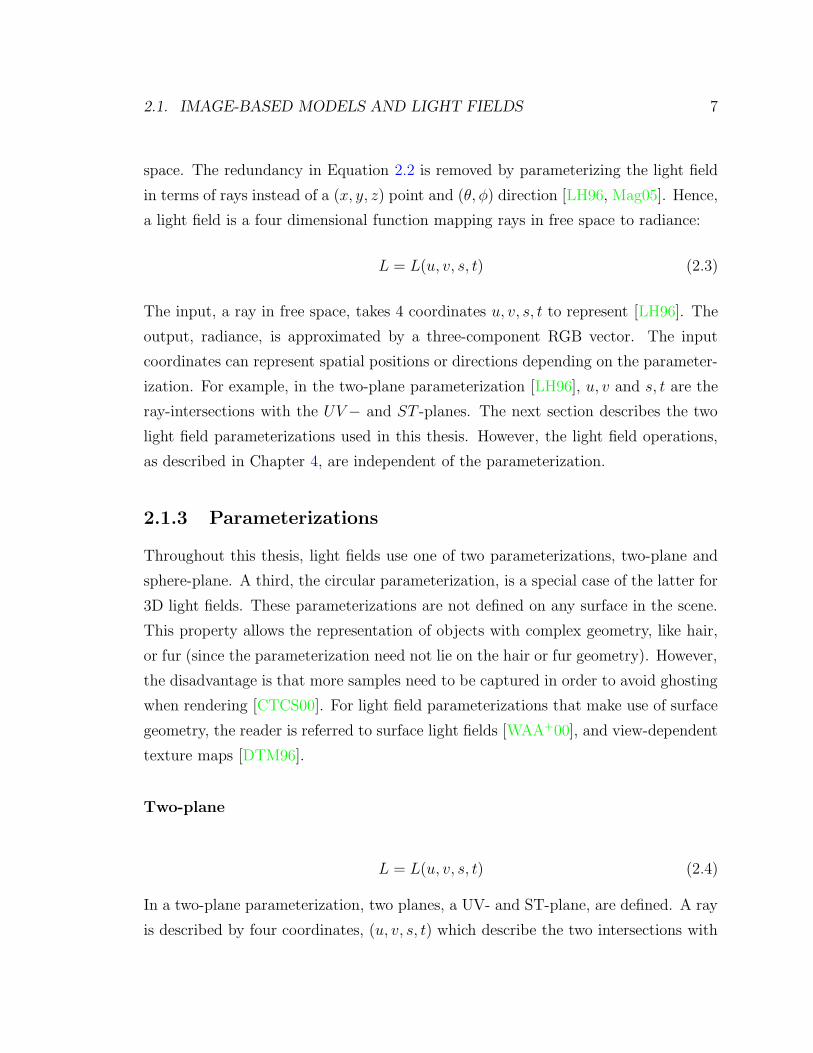
L = L(u, v, s, t) (2.3)
The input, a ray in free space, takes 4 coordinates u, v, s, t to represent [LH96]. The
output, radiance, is approximated by a three-component RGB vector. The input
coordinates can represent spatial positions or directions depending on the parameter-
ization. For example, in the two-plane parameterization [LH96], u, v and s, t are the
ray-intersections with the UV− and ST -planes. The next section describes the two
light field parameterizations used in this thesis. However, the light field operations,
as described in Chapter 4, are independent of the parameterization.
2.1.3 Parameterizations
Throughout this thesis, light fields use one of two parameterizations, two-plane and
sphere-plane. A third, the circular parameterization, is a special case of the latter for
3D light fields. These parameterizations are not defined on any surface in the scene.
This property allows the representation of objects with complex geometry, like hair,
or fur (since the parameterization need not lie on the hair or fur geometry). However,
the disadvantage is that more samples need to be captured in order to avoid ghosting
when rendering [CTCS00]. For light field parameterizations that make use of surface
geometry, the reader is referred to surface light fields [WAA+00], and view-dependent
texture maps [DTM96].
Two-plane
L = L(u, v, s, t) (2.4)
In a two-plane parameterization, two planes, a UV- and ST-plane, are defined. A ray
is described by four coordinates, (u, v, s, t) which describe the two intersections with

8 CHAPTER 2. BACKGROUND
the UV- and ST-plane. This is a natural parameterization for datasets acquired from
an array of cameras. The UV-plane is defined as the plane on which the cameras
lie. The ST-plane is the plane on which all camera images are rectified. Images
are rectified by capturing a light field of a planar calibration target and computing
homographies to a user-selected camera image [VWJL04].
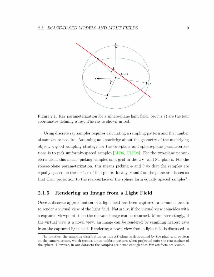
Sphere-plane
L = L(φ, θ, s, t) (2.5)
The sphere-plane light field parameterization (SLF) uses a different set of four coor-
dinates. A sphere with radius R surrounds the object represented by the light field.
A ray is parameterized by two intersections, (φ, θ) and (s, t). The first is the closest
intersection with the sphere. This is parameterized using spherical coordinates; φ is
the angle from the vertical axis of the sphere and θ is the rotation angle around the
vertical axis. The second intersection, parameterized by (s, t), is on a plane that
is incident to the center of the sphere, with normal N . Figure 2.1 illustrates this
parameterization.
A special case of the SLF for 3D light fields is the circular parameterization, which
fixes φ to 90◦. The fish, teddy bear and toy warrior light fields listed in Table A.1
use this parameterization.
2.1.4 A Discrete Approximation to the Continuous Light
Field
Given the two parameterizations described above, acquisition systems discretely sam-
ple the continuous light field with ray samples. In practice, these discrete samples
are acquired from captured photographs. Assuming that cameras are pinhole devices,
each photograph measures the radiance along a bundle of rays converging to the cen-
ter of projection of the camera. If multiple photographs are captured from different
viewpoints, these images approximate the continuous light field.
2.1. IMAGE-BASED MODELS AND LIGHT FIELDS 9
θ
(s,t)
φ
y
x
z
Figure 2.1: Ray parameterization for a sphere-plane light field. (φ, θ, s, t) are the fourcoordinates defining a ray. The ray is shown in red.
Using discrete ray samples requires calculating a sampling pattern and the number
of samples to acquire. Assuming no knowledge about the geometry of the underlying
object, a good sampling strategy for the two-plane and sphere-plane parameteriza-
tions is to pick uniformly-spaced samples [LH96, CLF98]. For the two-plane param-
eterization, this means picking samples on a grid in the UV- and ST-planes. For the
sphere-plane parameterization, this means picking φ and θ so that the samples are
equally spaced on the surface of the sphere. Ideally, s and t on the plane are chosen so
that their projection to the rear-surface of the sphere form equally spaced samples1.
2.1.5 Rendering an Image from a Light Field
Once a discrete approximation of a light field has been captured, a common task is
to render a virtual view of the light field. Naturally, if the virtual view coincides with
a captured viewpoint, then the relevant image can be returned. More interestingly, if
the virtual view is a novel view, an image can be rendered by sampling nearest rays
from the captured light field. Rendering a novel view from a light field is discussed in
1In practice, the sampling distribution on this ST -plane is determined by the pixel grid patternon the camera sensor, which creates a non-uniform pattern when projected onto the rear surface ofthe sphere. However, in our datasets the samples are dense enough that few artifacts are visible.
10 CHAPTER 2. BACKGROUND
more detail in [LH96, GGSC96, BBM+01]. This process of rendering an image from
a light field has numerous names, including “light field sampling,” “rendering from a
light field,” “novel view synthesis,” and “extracting a 2D slice”.
2.2 Acquisition Systems
Historically, a major hurdle in the use of light fields is acquiring dense samples to
approximate the continuous function shown in Equation 2.3. Fortunately, recent ad-
vances in camera technology combined with novel uses of optics have made acquisition
not only a practical task, but also a cheap and potentially common one as well. As
light fields become more common, users will want to interact with them as they do
with images and traditional 3D models.
Early acquisition systems made use of mechanical gantries to acquire light fields.
A camera is attached to the end of the gantry arm and the arm is moved to multiple
positions. Two useful gantry configurations are the planar and spherical ones. In
a planar configuration, the end effector of the gantry arm moves within a plane,
enabling acquisition of two-plane parameterized light fields. One example is the
gantry [Lev04a] used to acquire 3D scans of Michelangelo’s David [LPC+00] and a
light field of the statue of Night. This gantry is used to acquire several two-plane
light fields listed in Table A.1. In a spherical configuration, the end-effector travels
on the surface of a sphere, enabling acquisition of circular and spherical light fields.
The Stanford Spherical Gantry [Lev04b] is one example. This gantry is also used to
acquire the sphere-plane and circular light fields in Table A.1. While these gantries
can capture a dense sampling of a light field, they assume a static scene, are bulky,
and are costly. The Stanford Spherical Gantry costs $130,000.
To capture dynamic scenes, researchers have built arrays of cameras. The ability
to acquire dynamic scenes enables the acquisition of complex objects like human
actors. Manex Entertainment first popularized this technique in the movie, The
Matrix. During one scene, the actress appears to freeze while the camera moves
around her. This effect, now coined the “Matrix effect” or “bullet-time,” was created
by simultaneously triggering an array of cameras, and rendering images from the

2.2. ACQUISITION SYSTEMS 11
captured photographs.
Other camera arrays include the video camera array in the Virtualized Reality
Project at CMU [RNK97] , the 8x8 webcam array at MIT [YEBM02], the 48 pan-
translation camera array [ZC04], and the Stanford Multi-camera Array [WJV+05,
WSLH02]. This thesis uses several datasets captured using the Stanford Multi-camera
Array. With the exception of the webcam array, each system is costly and makes use
of specialized hardware. Furthermore, arrays like the Stanford Multi-camera Array
generally span a large area (3 x 2 meters), which makes it challenging to move. These
acquisition devices are useful in a laboratory setting, but have limited use in everyday
settings.
To build mobile and cheap acquisition devices, researchers have exploited optics
to trade off the spatial resolution of a single camera for multiple viewpoints of a scene.
One of the first techniques is integral photography, in which a fly’s-eye lens sheet is
placed in front of a sensor array, thereby allowing the array to capture the scene from
many viewpoints [Oko76]. The total image is composed of tiny images, each with a
different viewpoint. Today, such images are created by embedding lenses within a
camera body [NLB+05] or a lens encasement [GZN+06]. This thesis contains light
fields captured from the hand-held light field camera built by Ng et al. In [GZN+06],
they construct a lens encasement containing 20 lenses. Each lens provides a different
viewpoint of the scene. The lens encasement is attachable to any conventional SLR
camera. A light field is captured simply by pressing the shutter button. Acquisition
devices such as this are mobile, cheap, and easy to use. As such devices become
common, light fields will become abundant and users will want to manipulate this
data type as they do with images and 3D objects. The first contribution of this thesis
is a novel way to manipulate these light fields, described in Chapter 3.

12 CHAPTER 2. BACKGROUND
Chapter 3
Light Field Deformation
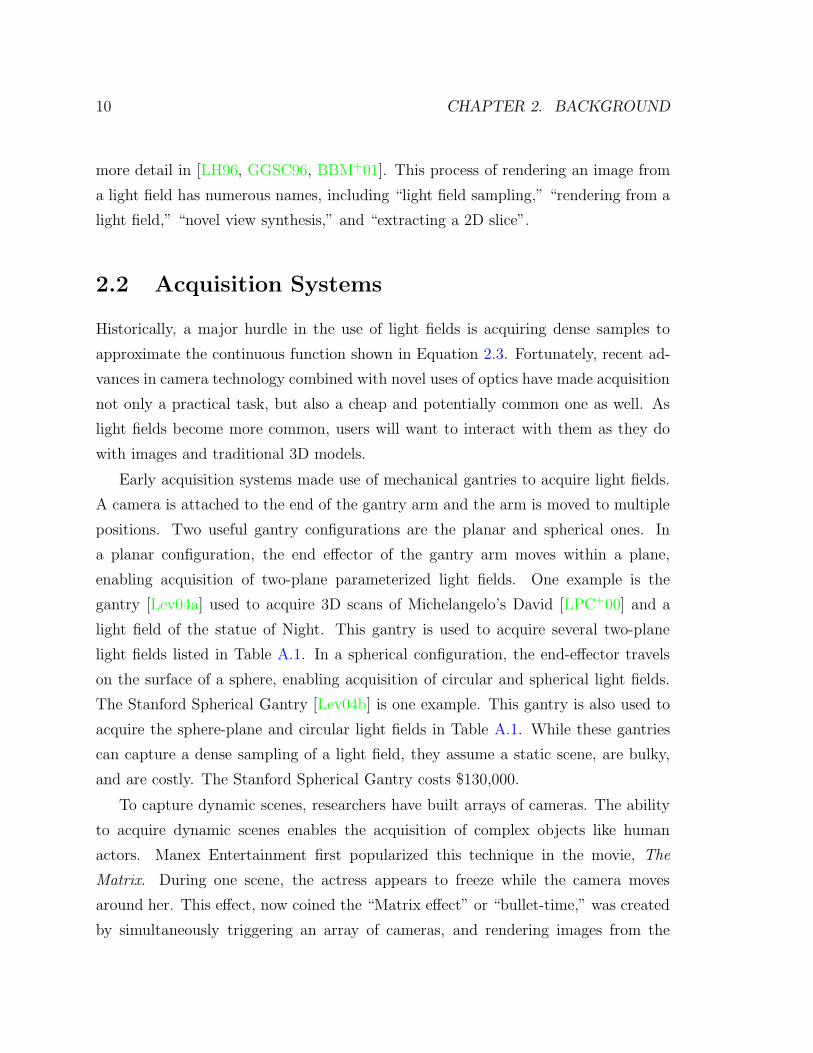
The first contribution of this thesis is a novel way to manipulate light fields, by
approximating object deformation. An animator can then “breathe life” into objects
represented by light fields. Our goal is similar to cartoon animation; the final result is
a deformed object, but the object need not be physically plausible, volume-preserving,
or “water-tight”. Figure 3.1 illustrates a deformation that twists a light field of a toy
Terra Cotta Warrior.
Figure 3.1: Light field deformation enables an animator to interactively deform photo-realistic objects. The left figure is an image from a light field of a toy Terra CottaWarrior. The middle image shows a view of the light field after applying a deforma-tion, in this case, a twist to the left. Notice that his feet remain fixed and his rightear now becomes visible. The right image shows the warrior turning to his right.Animating the light field in this way makes it appear alive and dynamic, propertiesnot commonly associated with light fields.
13

14 CHAPTER 3. LIGHT FIELD DEFORMATION
In order to deform a light field there are two core problems that need to be
solved. The first is specifying a transformation on the rays of the light field so that
it approximates a change in shape. The second is ensuring that the illumination
conditions after deformation remain consistent.
For the first problem, recall from Chapter 2 that a light field is a 4D function
mapping rays to RGB colors. In practice, this 4D function is approximated by a
set of images. In other words, a light field can be thought of as a set of rays, or a
set of pixels. An object represented by a light field is composed of these rays. The
goal is to specify a transformation that maps rays in the original light field to rays
in a deformed light field. Many ray-transformations exist, but we seek a mapping
that approximates a change in the shape of the represented object. For example,
a simple ray-transformation can be constructed by exploiting the linear mapping of
3D points. If we represent this mapping as a 4x4 matrix and represent 3D points in
homogeneous coordinates, then to deform the light field we simply take each ray, pick
two points along that ray, apply the 4x4 matrix to both points, and form a new ray
from the two transformed points. This ray-transformation simulates a homogeneous
transformation on the object represented by the light field. In this chapter, we present
a ray-transformation that can intuitively express Euclidean, similarity, and affine
transformations. This transformation can also simulate the effect of twisting the 3D
space in which an object is embedded, an effect that is difficult with a projective
transformation.
The second problem to deformation is related to the property that the RGB color
along any ray in a light field is a function of the illumination condition. When a
ray is transformed, the illumination condition is transformed along with the ray.
When multiple rays are transformed, this can produce an overall illumination that is
different than the original. For example, consider a light field of a scene with a point
light and a flat surface. Consider a ray r that is incident to a point on the surface.
The incident illumination makes an angle with respect to r. If we transform r, the
illumination angle remains fixed, relative to r. This causes the apparent illumination
to differ from the original light direction. The goal is to provide a way to ensure
that after deformation, the illumination remains consistent to the original lighting

3.1. PREVIOUS WORK: 3D RECONSTRUCTION FOR DEFORMATION 15
conditions. To solve this problem, a special kind of light field, called a coaxial light
field is captured.
These two problems are not new. Previous approaches avoid the two problems of
specifying a ray-transform and preserving illumination by attempting to reconstruct
a 3D model based on the input images1. Hence, an accurate 3D model is necessary.
The solution presented in this thesis avoids building an explicit model and provides
a solution for maintaining a specific form of illumination during deformation.
3.1 Previous Work: 3D Reconstruction for Defor-
mation
Previous approaches reconstruct geometry, surface properties and illumination using
the images from the light field. Then the geometry is deformed by displacing mesh
vertices. The deformed object can then be re-rendered. However, reconstructing a
geometry from images is a difficult problem in computer vision. Nevertheless, several
techniques exist, including multi-baseline stereo [KS96] and voxel coloring [SK98].
Assuming that a 3D model can be constructed, reflectance properties are then
estimated. In [SK98], they assume the object is diffuse. Meneveaux and Fournier
discuss a system that can make use of more complex reflectance properties [MSF02].
The reflectance properties can also be represented in a sampled form, as is shown by
Weyrich et al., in which they capture and deform a surface reflectance field [WPG04].
Knowing the surface properties and geometry is sufficient to keep the apparent il-
lumination consistent after object deformation. Once the mesh vertices have been
deformed, the appearance of that part of the mesh can be rendered using the local
surface normal, incident light direction and view direction.
This approach is successful as long as geometry, surface properties, and illumi-
nation can be accurately modeled. Unfortunately, this assumption fails for many
interesting objects for which light fields are commonly used, like furry objects. The
1One approach, used in light field morphing [ZWGS02], avoids 3D reconstruction and instead in-duces a ray-transformation between two input light fields by specifying corresponding rays. However,they do not address the problem of inconsistent illumination.

16 CHAPTER 3. LIGHT FIELD DEFORMATION
approach presented in this thesis avoids explicit reconstruction and presents a tech-
nique for keeping illumination consistent and for specifying a ray-transformation.
3.2 Solving the Illumination Problem
In introducing our technique for light field deformation, we first address the problem
of maintaining consistent illumination during a transformation of the rays of a light
field. Then, we discuss how a transformation can be specified by an animator in an
intuitive, interactive manner.
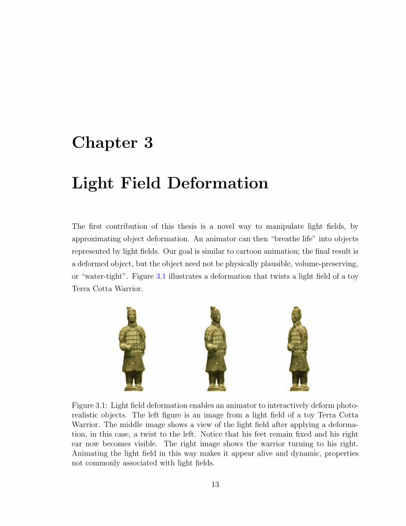
To understand the illumination problem that arises when transforming the rays
of a light field, consider the scene shown in Figure 3.2. A point light is located at
infinity, emitting parallel light rays onto a lambertian, checkerboard surface. A light
field of this checkerboard is captured. Two rays of this light field are shown as black,
vertical arrows. The corresponding light direction for these two rays is shown in
yellow. Notice that since both rays of the light field are vertical and the illumination
is distant, the angle between the illumination ray and the light field ray is φ. The key
idea is that no matter how a ray is transformed, the color along that ray direction
will be as if the illumination direction had made an angle φ to the ray.
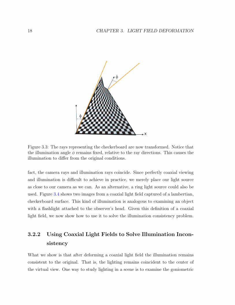
Figure 3.3 shows the illumination directions for the two rays of the light field after
transforming the upper-right ray. Notice that the illumination direction maintains an
angle φ with the ray direction. However, the two illumination directions are no longer
parallel. The illumination after transforming the rays is different than the original.
Because the color along a ray is a function of the relative angle between the
illumination and the ray, after transforming this ray the illumination direction points
in a different direction. In most cases, this means that when a light field is deformed
(e.g. all its rays are transformed), the apparent illumination will also change. To
solve this problem, we capture a new kind of light field, called a coaxial light field,
which maintains lighting consistency during deformation but still captures interesting
shading effects.
3.2. SOLVING THE ILLUMINATION PROBLEM 17
Figure 3.2: A lambertian scene with distant lighting. The checkerboard surface is litby a point light located at infinity. Two rays of the light field are shown in black.They make an angle φ with respect to the illumination direction.
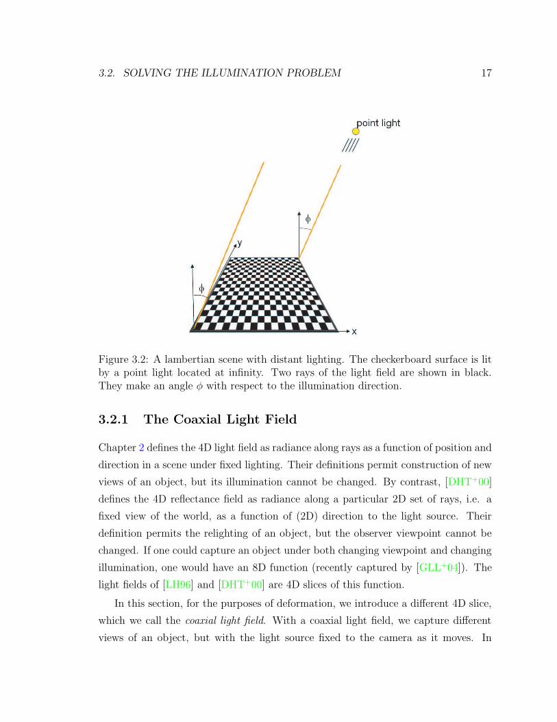
3.2.1 The Coaxial Light Field
Chapter 2 defines the 4D light field as radiance along rays as a function of position and
direction in a scene under fixed lighting. Their definitions permit construction of new
views of an object, but its illumination cannot be changed. By contrast, [DHT+00]
defines the 4D reflectance field as radiance along a particular 2D set of rays, i.e. a
fixed view of the world, as a function of (2D) direction to the light source. Their
definition permits the relighting of an object, but the observer viewpoint cannot be
changed. If one could capture an object under both changing viewpoint and changing
illumination, one would have an 8D function (recently captured by [GLL+04]). The
light fields of [LH96] and [DHT+00] are 4D slices of this function.
In this section, for the purposes of deformation, we introduce a different 4D slice,
which we call the coaxial light field. With a coaxial light field, we capture different
views of an object, but with the light source fixed to the camera as it moves. In
18 CHAPTER 3. LIGHT FIELD DEFORMATION
Figure 3.3: The rays representing the checkerboard are now transformed. Notice thatthe illumination angle φ remains fixed, relative to the ray directions. This causes theillumination to differ from the original conditions.
fact, the camera rays and illumination rays coincide. Since perfectly coaxial viewing
and illumination is difficult to achieve in practice, we merely place our light source
as close to our camera as we can. As an alternative, a ring light source could also be
used. Figure 3.4 shows two images from a coaxial light field captured of a lambertian,
checkerboard surface. This kind of illumination is analogous to examining an object
with a flashlight attached to the observer’s head. Given this definition of a coaxial
light field, we now show how to use it to solve the illumination consistency problem.
3.2.2 Using Coaxial Light Fields to Solve Illumination Incon-
sistency
What we show is that after deforming a coaxial light field the illumination remains
consistent to the original. That is, the lighting remains coincident to the center of
the virtual view. One way to study lighting in a scene is to examine the goniometric

3.2. SOLVING THE ILLUMINATION PROBLEM 19
Figure 3.4: Two images from a coaxial light field. The lighting is a point light sourceplaced at the center of projection of the camera. As the camera moves to an obliqueposition (right), the checkerboard is dimmed due to the irradiance falling off with theangle between the lighting direction and the surface normal.
diagram at a differential patch on a lambertian surface. A goniometric diagram plots
the distribution of reflected radiance over the local bundle of rays incident to that
patch2. In a goniometric diagram, the length of the plotted vectors is proportional to
the reflected radiance quantity in that direction. Since the patch is on a lambertian
surface, it reflects light equally in all directions (e.g. the diagram is not biased in
any direction by the reflectance properties). Thus the shape and size of the diagram
gives us insight into the illumination condition. For example, under fixed lighting
a goniometric diagram of a patch on a lambertian surface has the shape of a semi-
circle. This is because the lambertian surface reflects radiance equally in all directions.
Furthermore, the radius of the semi-circle is a function of the angle between the surface
normal and the illumination direction.
Now let us examine the goniometric diagram corresponding to coaxial lighting.
Let us return to Figure 3.4 which shows a checkerboard captured by a coaxial light
field. Consider two differential patches A1 and A2 on the checkerboard. Figure 3.5
shows the associated goniometric diagrams. Compared to fixed lighting, the diagrams
indicate that reflected radiance is now a function of the reflection angle.
Described mathematically, because the surface is lambertian the radiance R can
2Some goniometric diagrams are drawn as a function of radiant intensity. However, we felt thatplotting radiance provides a more intuitive notion of the reflected “light energy”.
20 CHAPTER 3. LIGHT FIELD DEFORMATION
be described as a function of the light direction L and the surface normal N [CW93]:
R = ρE = ρIN • L
r2(3.1)
where ρ is the BRDF for a diffuse surface, E is irradiance, I the radiant intensity of
the point light and r the distance from the light to the patch.
Since the illumination is coaxial, any ray V from the patch has coaxial illumina-
tion, e.g. V = L. If we substitute this equality into Equation 3.1,
R = ρIN • V
r2(3.2)
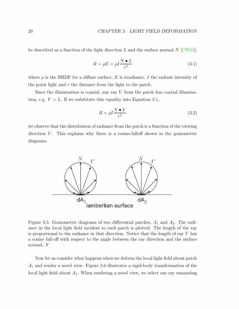
we observe that the distribution of radiance from the patch is a function of the viewing
direction V . This explains why there is a cosine-falloff shown in the goniometric
diagrams.
Figure 3.5: Goniometric diagrams of two differential patches, A1 and A2. The radi-ance in the local light field incident to each patch is plotted. The length of the rayis proportional to the radiance in that direction. Notice that the length of ray V hasa cosine fall-off with respect to the angle between the ray direction and the surfacenormal, N
Now let us consider what happens when we deform the local light field about patch
A1 and render a novel view. Figure 3.6 illustrates a rigid-body transformation of the
local light field about A1. When rendering a novel view, we select one ray emanating

3.2. SOLVING THE ILLUMINATION PROBLEM 21
from A1 and one ray from A2. In both rays, the radiance along those directions have
coaxial illumination. Only one illumination condition satisfies this constraint: a point
light source located at the virtual viewpoint. This illumination is consistent with the
initial conditions before deforming the rays.
Figure 3.6: Goniometric diagrams of two differential patches, A1 and A2, after trans-forming the rays from A1. When a novel view is rendered by sampling rays fromthe two diagrams, notice that the radiance along L1 has coaxial illumination (shownin red). Similarly, the radiance along L2 has coaxial illumination. The only plausi-ble illumination condition for these constraints is a point light located at the virtualviewpoint.
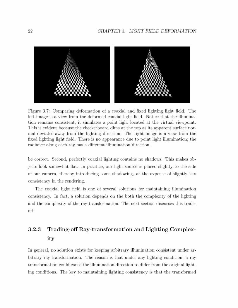
For comparison, Figure 3.7 shows novel views after deforming a coaxial and fixed-
illumination light field. Only the coaxial light field generates a correct rendering of
the deformed checkerboard.
Thus, the advantage of using coaxial light fields is that it ensures the correct
appearance of objects under deformation, even though no geometry has been cap-
tured. However, coaxial light fields have several limitations. First, the object must
be diffuse; specular highlights will look reasonable when deformed, but they will not
22 CHAPTER 3. LIGHT FIELD DEFORMATION
Figure 3.7: Comparing deformation of a coaxial and fixed lighting light field. Theleft image is a view from the deformed coaxial light field. Notice that the illumina-tion remains consistent; it simulates a point light located at the virtual viewpoint.This is evident because the checkerboard dims at the top as its apparent surface nor-mal deviates away from the lighting direction. The right image is a view from thefixed lighting light field. There is no appearance due to point light illumination; theradiance along each ray has a different illumination direction.
be correct. Second, perfectly coaxial lighting contains no shadows. This makes ob-
jects look somewhat flat. In practice, our light source is placed slightly to the side
of our camera, thereby introducing some shadowing, at the expense of slightly less
consistency in the rendering.
The coaxial light field is one of several solutions for maintaining illumination
consistency. In fact, a solution depends on the both the complexity of the lighting
and the complexity of the ray-transformation. The next section discusses this trade-
off.
3.2.3 Trading-off Ray-transformation and Lighting Complex-
ity
In general, no solution exists for keeping arbitrary illumination consistent under ar-
bitrary ray-transformation. The reason is that under any lighting condition, a ray
transformation could cause the illumination direction to differ from the original light-
ing conditions. The key to maintaining lighting consistency is that the transformed

3.3. SPECIFYING A RAY TRANSFORMATION 23
ray must have an associated lighting direction that is consistent with the original
illumination3. Therefore, the simpler the ray-transform, the more complex the light-
ing can be, and vice-versa. A trivial example is the identity transform. Under this
ray-mapping, the illumination can be arbitrarily complex. The equivalent trivial ex-
ample for lighting is ambient lighting4. In this case the ray-transform can be arbitrary
complex. Both these cases maintain lighting consistency. Something between triv-
ial lighting and trivial ray-transformation is if the illumination is distant (and hence
has parallel illumination directions). In this case any pure translation will preserve
lighting.
Given this trade-off for preserving lighting during ray-transformation, we chose
coaxial lighting because it has reasonable illumination properties and preserves coaxial
illumination during transformation. The next section discusses the details of the
actual ray-transformation.
3.3 Specifying a Ray Transformation
The second problem to light field deformation is specifying a ray transformation. Our
goal is to enable an animator to artistically express motion and feeling using light
fields.
There are many ways to specify a transformation on rays. For example, in the
beginning of this chapter, a 4x4 matrix was used to specify a rigid-body transfor-
mation. However, specifying a matrix is not intuitive for an animator. Instead, we
borrow a technique from the animation community for specifying transformations on
traditional 3D models (e.g. with mesh geometry). We adapt it to transform light
fields. The technique is called free-form deformation [SP86]. We first introduce the
original technique, then adapt it to deform light fields.
3Here, we ignore global illumination effects like self-shadowing, and inter-reflection.4In computer graphics, ambient lighting is a constant term added to all lighting calculations for
an object. In reality, the ambient lighting is a composition of all indirect illumination. The trivialcase being considered is if the object is only lit by ambient lighting, and hence has uniform lightingfrom all directions.

24 CHAPTER 3. LIGHT FIELD DEFORMATION
3.3.1 Free-form Deformation
In a traditional free-form deformation (FFD) [SP86], a deformation box C is defined
around a mesh geometry. The animator deforms C to form Cw, a set of eight displaced
points defining a deformed box5. The free-form deformation D is a 3D function
mapping C, the original box, to Cw, the deformed one:
D : <3 → <3 (3.3)
More importantly, D is used to warp all points inside the box C.
How is D parameterized? In the original paper by Sederberg and Parry, D is
represented by a trivariate tensor product Bernstein polynomial. The details of their
formulation of D are unimportant for deforming light fields. The key idea is that
we use their method for specifying a deformation. That is, an animator manipulates
a deformation box to specify a warp. The difference is that while the original FFD
warps 3D points, our formulation warps rays.
To make use of the FFD paradigm, we first define a function that makes use of
the deformation box to warp 3D points. We will prove that this function does not
preserve straight lines, so we modify it to warp ray parameters instead of 3D points.
This modified form will be the final ray warp. Let us begin by introducing the 3D
warping function, parameterized by trilinear interpolation.
3.3.2 Trilinear Interpolation
To introduce trilinear interpolation, assume that a deformation box (e.g. a rectan-
gular parallelepiped) is defined with 8 vertices, ci, i = 1 . . . 8. These 8 vertices also
define three orthogonal basis vectors, U , V , and W . The origin of these basis vectors
is X0, one of the vertices of the box. Then for any 3D point p, Equation 3.4 defines
coordinates, u, v, and w:
u = V ×W ·(X−X0)V ×W ·U
v = U×W ·(X−X0)U×W ·V
w = U×V ·(X−X0)U×V ·W
(3.4)
5One assumption is that the animator does not move points to form self-intersecting polytopes.

3.3. SPECIFYING A RAY TRANSFORMATION 25
By trilinearly interpolating across the volume, p can be described in terms of the
interpolation coordinates and the 8 vertices of the cube:
p = (1− u)(1− v)(1− w)c1 + (u)(1− v)(1− w)c2 +
(1− u)(v)(1− w)c3 + (u)(v)(1− w)c4 +
(1− u)(1− v)(w)c5 + (u)(1− v)(w)c6 +
(1− u)(v)(w)c7 + (u)(v)(w)c8
(3.5)
Given the trilinear coordinates u, v, w for a point p, the transformed point is
computed using Equation 3.5 and the points in Cw substituted for ci. Any 3D point
can be warped using this technique.
Unfortunately, this technique does not preserve straight lines. To observe this
property, without loss of generality let us examine the bilinear interpolation case and
consider the deformation shown in Figure 3.8. Three collinear points a, b and c are
transformed. We test for collinearity by forming a line between two points (in this
case, a and c) and showing that the third point lies on the line:
ax + by + c = 0 (line in standard form) (3.6)
−x + y = 0 (line through a and c) (3.7)
1− 1 = 0 (substituting b) (3.8)
We show that after transformation, a′, b′ and c′ are no longer collinear. After
bilinear interpolation,
a′ =
0
0
b′ =
23109
c′ =
3
4
(3.9)
The line formed from a′ and c′ is:
4
3x− y = 0 (3.10)
26 CHAPTER 3. LIGHT FIELD DEFORMATION
a (0,0)
b (1,1)
c (3,3)
a‘ (0,0)
c‘ (3,4)
b‘ ( , )2
3
10
9
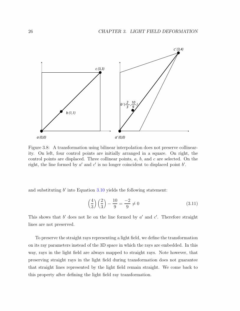
Figure 3.8: A transformation using bilinear interpolation does not preserve collinear-ity. On left, four control points are initially arranged in a square. On right, thecontrol points are displaced. Three collinear points, a, b, and c are selected. On theright, the line formed by a′ and c′ is no longer coincident to displaced point b′.
and substituting b′ into Equation 3.10 yields the following statement:
(
4
3
) (
2
3
)
−10
9=−2
96= 0 (3.11)
This shows that b′ does not lie on the line formed by a′ and c′. Therefore straight
lines are not preserved.
To preserve the straight rays representing a light field, we define the transformation
on its ray parameters instead of the 3D space in which the rays are embedded. In this
way, rays in the light field are always mapped to straight rays. Note however, that
preserving straight rays in the light field during transformation does not guarantee
that straight lines represented by the light field remain straight. We come back to
this property after defining the light field ray transformation.

3.3. SPECIFYING A RAY TRANSFORMATION 27
3.3.3 Defining a Ray Transformation
The key idea in defining a ray transformation that preserves the straight rays of the
light field is to define the transformation in terms of the ray parameters. In this way,
rays are always mapped to straight rays. We use the two-plane parameterization of a
ray and factor the trilinear warp into two bilinear warps that displace the (u, v) and
(s, t) coordinates in the UV - and ST -plane, respectively.
First, to compute the location of the UV - and ST -planes and the (u, v, s, t) co-
ordinates for a ray, we intersect the ray of the light field6 with the deformation box
C. The two intersection planes define the UV - and ST -planes. The corresponding
intersection points define the (u, v, s, t) coordinates. In other words, the two planes
define the entrance and exiting plane for the ray as it travels through the deformation
box.
Next, a separate bilinear warp is applied to the (u, v) and (s, t) coordinates. Fac-
torizing the trilinear warp into two bilinear warps is advantageous for two reasons.
First, bilinearly warping in this way preserves straight rays representing the light
field. That is, the new light field is represented by a set of straight rays. Second, two
bilinear warps take 18 scalar multiplications of the coefficients. A single trilinear warp
takes 42 scalar multiplications. Therefore bilinear warps can be computed quicker.
The bilinear warp is a simplified version of Equation 3.5. The four interpolat-
ing points are those defining the UV - or ST -plane. This warp produces a new ray
(u′, v′, s′, t′) which is then re-parameterized to the original parameterization of the
light field. Figure 3.9 summarizes the algorithm for transforming a ray of the light
field. Figure 3.10 illustrates how a ray is transformed, pictorially.
3.3.4 Properties of the Ray Transformation
Given the above definition of a ray transformation, it is useful to compare it to other
transformations to understand its advantages and disadvantages. A common set of 3D
transformations is the specializations of a projective transformation. The projective
6The captured light field already has a ray parameterization, but needs to be re-parameterizedfor ray transformation.

28 CHAPTER 3. LIGHT FIELD DEFORMATION
transform ray (ray)1 ruvst ← reparameterize(ray)2 puv ← biwarp(ruv)3 pst ← biwarp(rst)4 quvst ← [puv, pst]5 return reparameterize original(quvst)
Figure 3.9: Algorithm for using bilinear interpolation to transform rays.
transformation is a group of invertible n x n matrices, related by a scalar multiplier.
In the case of transformations on 3D points, n = 4.
The projective transformation maps straight lines to straight lines [HZ00]. There-
fore, it is useful to compare our ray-transformation to it. We show that our ray-
transformation can define Euclidean, similarity, and affine transforms. Unfortunately,
as we will show, not all general projective transforms can be produced. However, we
show that our ray-transform can perform mappings beyond projective mappings, like
twisting.
Euclidean, Similarity, and Affine Transforms
A Euclidean transform models the motion of a rigid object; angles between lines,
length and area are preserved. If the object is also allowed to scale uniformly, then
this models a similarity transform; angles are still preserved, as well as parallel lines.
If an object can undergo non-isotropic scaling and rotation followed by a translation,
this transformation models an affine one7. Affine transforms preserve parallel lines,
ratios of lengths of parallel line segments, and ratios of areas.
Mathematically, these three transforms can be written in matrix form:
x′ = Tx =
A t
0 1
x (3.12)
where x and x′ are 4x1 vectors, T a 4x4 matrix, A a 3x3 matrix, t a 3x1 vector and
0 a 1x3 vector. If A = G, for orthogonal matrix G, then T is a Euclidean transform.
7It can be shown that an affine matrix can be factored into a rotation, a non-isotropic scaling,and another two rotations, followed by a translation [HZ00].
3.3. SPECIFYING A RAY TRANSFORMATION 29
UV
ST
UV
ST
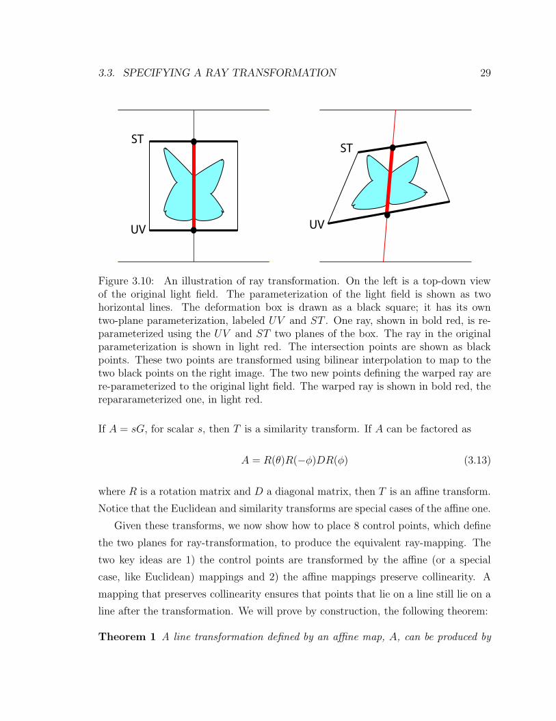
Figure 3.10: An illustration of ray transformation. On the left is a top-down viewof the original light field. The parameterization of the light field is shown as twohorizontal lines. The deformation box is drawn as a black square; it has its owntwo-plane parameterization, labeled UV and ST . One ray, shown in bold red, is re-parameterized using the UV and ST two planes of the box. The ray in the originalparameterization is shown in light red. The intersection points are shown as blackpoints. These two points are transformed using bilinear interpolation to map to thetwo black points on the right image. The two new points defining the warped ray arere-parameterized to the original light field. The warped ray is shown in bold red, therepararameterized one, in light red.
If A = sG, for scalar s, then T is a similarity transform. If A can be factored as
A = R(θ)R(−φ)DR(φ) (3.13)
where R is a rotation matrix and D a diagonal matrix, then T is an affine transform.
Notice that the Euclidean and similarity transforms are special cases of the affine one.
Given these transforms, we now show how to place 8 control points, which define
the two planes for ray-transformation, to produce the equivalent ray-mapping. The
two key ideas are 1) the control points are transformed by the affine (or a special
case, like Euclidean) mappings and 2) the affine mappings preserve collinearity. A
mapping that preserves collinearity ensures that points that lie on a line still lie on a
line after the transformation. We will prove by construction, the following theorem:
Theorem 1 A line transformation defined by an affine map, A, can be produced by

30 CHAPTER 3. LIGHT FIELD DEFORMATION
Projective
Affine
Euclidean
Similarity
Bilinear Ray Warp
Figure 3.11: A hierarchy of line/ray transformations. The bilinear ray-transformationintroduced in Section 3.3.3 can simulate up to affine transforms and a subset of theprojective ones. It can also perform line transformations that are impossible with theprojective transform, such as twisting.
the ray-transformation described in Section 3.3.3 by applying A to all 8 control points.
The proof is by construction. The ray-transform in Section 3.3.3 is specified by 8
control points, 4 defining the UV -plane and 4 for the ST -plane. We call the control
points, which are in homogeneous coordinates, a, b, c, . . . , h. The new control points
are defined as follows: a′ = Aa, b′ = Ab, c′ = Ac, . . . , h′ = Ah. In other words,
the new control points are simply the affine mappings of the original control points.
These control points will be used for the bilinear warp in the UV - and ST -planes
Given the displaced control points a′, . . .h′, we now show that any warped ray is
transformed in exactly the same way as the affine mapping. This is done by taking
2 points in the UV - and ST -planes, bilinearly warping them, and showing that these
3.3. SPECIFYING A RAY TRANSFORMATION 31
two new points are the same points using an affine warp. Furthermore, since the
affine warp preserves collinearity, the line formed by the two affinely warped points
is the same as the line made by connecting the bilinearly warped points on the UV -
and ST -planes.
Suppose we have a point Puv on the UV -plane:
Puv = (1− u)(1− v)a + (u)(1− v)b+
(1− u)(v)c + (u)(v)d(3.14)
where u and v are the interpolation coordinates on the UV -plane. Then using the
displaced control points, we can bilinearly interpolate the warped point for Puv:
P ′
uv = (1− u)(1− v)a′ + (u)(1− v)b′+
(1− u)(v)c′ + (u)(v)d′
(3.15)
But recall that a′ = Aa, b′ = Ab, c′ = Ac, . . . , h′ = Ah. Substituting this in:
P ′
uv = (1− u)(1− v)Aa + (u)(1− v)Ab+
(1− u)(v)Ac + (u)(v)Ad(3.16)
and factoring out A reveals:
P ′
uv = A[(1− u)(1− v)a + (u)(1− v)b + (1− u)(v)c + (u)(v)d] = APuv (3.17)
Equation 3.17 states that the bilinearly warped point P ′
uv can be computed by ap-
plying the affine warp A to Puv. A similar argument can be made for P ′
st = APst.
Since affine warps preserve collinearity of points, the affine warp has mapped any
line through Puv and Pst to a line through P ′
uv and P ′
st. This proves that any affine
mapping of lines can be produced by our ray-transform.
Tackling the General Projective Transform
Unfortunately, the proof-by-construction presented above does not apply to general
projective transforms. In Equation 3.17, suppose A is a projective transform of the

32 CHAPTER 3. LIGHT FIELD DEFORMATION
form:
x′ = Ax =
P t
vT s
x (3.18)
with 3x3 matrix P , 3x1 vector t, 3x1 vector v and scalar s. In this case, A can
not be factored out of the equation because there may be a different homogeneous
division for each term in the equation. This means that directly applying a projective
transform to the control points will not yield the same ray-transform as a projective
transform. Note that this was the case with the affine map. Figure 3.12 is a graphical
explanation of the projective transform. In this case, the transform is in flatland,
e.g. a 2D projective transform. What we’ve shown so far is that a bilinear ray-warp
constructed by projectively mapping the original control points does not produce
the same ray-warp. But can a different construction of the control points yield an
equivalent ray-warp? Unfortunately, the answer is no. The reason is simple. If
the control points are not projectively mapped, then warped rays between control
points will never match projectively warped rays. Therefore, for general projective
transforms, it is impossible to produce an equivalent bilinear ray warp.
Fundamentally, the 8 control points of the bilinear ray transform need to map
to the 8 projectively transformed points. If this is not the case, then rays formed
from opposing corners in the undeformed case will map to different rays when using
the bilinear and the projective warp. However, as shown in Figure 3.12 for the 2D
case, if the 4 control points coincide with the projectively warped points then rays
still do not match between bilinear and projective mappings. Therefore, for general
projective transforms, it is impossible to produce an equivalent bilinear ray warp.
Beyond Projective Transforms
Although the bilinear ray-transform cannot reproduce all projective transforms, it
has two nice properties that make it more useful for an animator. First, bilinear
ray-transforms can simulate the effect of twisting (like in Figure 3.1); projective
transforms can not. Twisting is a rotation of one of the faces of the deformation
box. Bilinear ray-warping handles this case as it normally handles any ray warp. 3D
projective transforms, however, cannot map a cube to a twisted one because some

3.3. SPECIFYING A RAY TRANSFORMATION 33
Figure 3.12: A 2D projective transform applied to lines on a checkerboard. On theleft, are the checkerboard lines before transformation. The checkerboard is a unitsquare, with the lower-left corner at the origin. Notice, the lines intersect the bordersof the checkerboard in a uniform fashion. On the right, are the checkerboard linesafter a projective transform. The projective transformation has translated the top-left corner to (0, 0.5) and the top right corner to (0.5, 1) Notice, that the intersectionsare no longer uniform along the borders. In our ray-transformation, the uniformly-spaced intersections on the left image map to uniform intersections on the right image(this is also true in the affine case because parallel lines are preserved). However, theprojective transform does not preserve this property for the borders, shown on theright.
of the sides of the box are no longer planar. Projective transforms preserve planes:
any four points that lie on a plane must lie on the same plane after the transforma-
tion8. Because of this invariant, projective transforms cannot represent ray warps
that involve bending the sides of the deformation box, like twisting. However, this
ray transformation is useful for an animator to produce twisting effects on toys or
models.
The trade-off is that the bilinear ray-transform no longer preserves straight lines
within the scene represented by the light field. Although this transform keeps the
rays of the light field straight after warping, lines in the scene represented by the
8The proof is a simple extension of the 2D version (that preserves lines), described in Theorem2.10 of [HZ03].
34 CHAPTER 3. LIGHT FIELD DEFORMATION
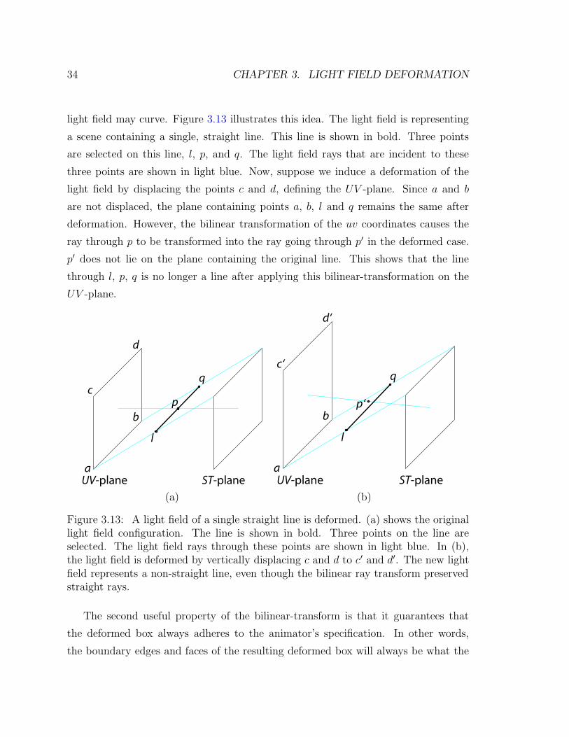
light field may curve. Figure 3.13 illustrates this idea. The light field is representing
a scene containing a single, straight line. This line is shown in bold. Three points
are selected on this line, l, p, and q. The light field rays that are incident to these
three points are shown in light blue. Now, suppose we induce a deformation of the
light field by displacing the points c and d, defining the UV -plane. Since a and b
are not displaced, the plane containing points a, b, l and q remains the same after
deformation. However, the bilinear transformation of the uv coordinates causes the
ray through p to be transformed into the ray going through p′ in the deformed case.
p′ does not lie on the plane containing the original line. This shows that the line
through l, p, q is no longer a line after applying this bilinear-transformation on the
UV -plane.
a
b
c
d
l
p
q
UV-plane ST-plane UV-plane ST-planea
b
c‘
d‘
l
p‘
q
(a) (b)
Figure 3.13: A light field of a single straight line is deformed. (a) shows the originallight field configuration. The line is shown in bold. Three points on the line areselected. The light field rays through these points are shown in light blue. In (b),the light field is deformed by vertically displacing c and d to c′ and d′. The new lightfield represents a non-straight line, even though the bilinear ray transform preservedstraight rays.
The second useful property of the bilinear-transform is that it guarantees that
the deformed box always adheres to the animator’s specification. In other words,
the boundary edges and faces of the resulting deformed box will always be what the

3.4. IMPLEMENTING THE RAY TRANSFORMATION 35
animator specifies. In contrast, when using a projective transform the deformed box
may not be exactly the same as what the animator specified. This is a useful property
when specifying multiple adjacent deformation boxes.
In summary, our analysis of the bilinear ray-transform shows that it can reproduce
up to affine mappings of rays. It cannot reproduce all projective mappings, but can
produce other effects, like twisting, which are impossible for projective transforms.
Furthermore, a bilinear ray-transform is guaranteed to adhere to the eight new control
points specified by the animator. This enables an intuitive method for specifying a
ray-transformation of the light field. Next we discuss how the bilinear ray transform
is implemented to enable interactive light field deformation.
3.4 Implementing the Ray Transformation
The ray transformation discussed so far warps all rays of the light field. The problem
is that light fields are dense, so transforming every ray is a time consuming process.
A typical light field has over 60 million rays (see Appendix A). Applying a transfor-
mation to all 60 million rays prevents interactive deformation. Instead, we exploit the
fact that at any given time, an animator only needs to see a 2D view of the deformed
light field, e.g. never the entire dataset. This means that we only need to warp the
view rays of the virtual camera. In other words, we deform rays “on demand” to
produce an image from the desired view point.
How are the warps on the light field and the warps on the view rays related? The
two warps are in fact inverses of each other, as shown in [Bar84]. For example, to
translate an object to the left, one can either apply a translation to the object, or
apply the inverse translation (i.e. translate to the right) to the viewing camera.
Therefore, to render an image from a deformed light field, we apply the inverse
ray warp to the view rays of the virtual camera. Given a view ray in the deformed
space, we need to find the pre-image (e.g. ray) in the undeformed space such that
warping the pre-image yields the given view ray. To find the pre-image of a ray, we
forward warp many rays, and interpolate amongst nearby rays. Figure 3.14 illustrates
this interpolation in ray space.

36 CHAPTER 3. LIGHT FIELD DEFORMATION
In the actual implementation, we use texture-mapping to help us forward-warp
many ray samples and interpolate amongst them. Recall from Section 3.3.3 that a
ray transformation is defined by 8 control points defining a deformation box (e.g.
two planes in the UV ST parameterization). To forward warp many ray samples, we
simply create many samples on the UV - and ST -planes and bilinearly warp them. To
interpolate between UV - and ST -samples, we triangulate the points and use barycen-
tric coordinates to shade each triangle. In this way, the texture color codes the original
coordinates of each UV and ST point. We used 64 x 64 x 2 textured triangles per
plane for our datasets. Figure 3.15 shows the UV -planes (left) and ST -planes (right)
for a deformation box.
U
S
U
S
ray warp
undeformed space deformed space
Figure 3.14: A pre-image of a ray is found by computing the forward warp for manysample rays, and interpolating amongst nearest rays. The above two diagrams are 2Dray-space diagrams illustrating the undeformed space (left) and the deformed space(right). Rays in ray-space are represented as points. The pre-image of the ray inthe deformed space (shown in red) is found by computing the nearest rays (shownin green), finding their counterparts in the undeformed space, and interpolating theoriginal ray positions. The interpolation is represented by the black lines. The pre-image is shown in blue in the undeformed space.

3.5. RESULTS 37
Figure 3.15: An inverse warp is approximated by forward warping many ray samplesand then interpolating the results. We use a hardware-accelerated texture-mappingapproach to quickly interpolate among the ray samples.
3.5 Results
We now present results illustrating how the bilinear ray-transform is used to intu-
itively specify a ray-transformation on the light field. This ray-transformation simu-
lates the effect of deforming the object represented by the light field. The animations
can be found at the following webpage:
http://graphics.stanford.edu/papers/bchen_thesis .
Figure 3.1 at the beginning of this chapter illustrates a twisting effect on the
light field. Figure 3.16 shows the associated deformation box for the twisted soldier.
The twisting of the deformation box is impossible for a projective transform. Figure
3.17 illustrates a bilinear ray-transform that simulates an affine ray warp. The user
supplies a deformation by moving vertices of the box (shown in gray) to a deformed
position (shown in red).
In these results so far, the deformation is global and lacks local control. In contrast,
an animator typically applies multiple deformations to a single object. In the next
section, we introduce a technique for applying multiple, independent ray transforms
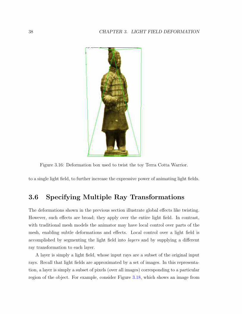
38 CHAPTER 3. LIGHT FIELD DEFORMATION
Figure 3.16: Deformation box used to twist the toy Terra Cotta Warrior.
to a single light field, to further increase the expressive power of animating light fields.
3.6 Specifying Multiple Ray Transformations
The deformations shown in the previous section illustrate global effects like twisting.
However, such effects are broad; they apply over the entire light field. In contrast,
with traditional mesh models the animator may have local control over parts of the
mesh, enabling subtle deformations and effects. Local control over a light field is
accomplished by segmenting the light field into layers and by supplying a different
ray transformation to each layer.
A layer is simply a light field, whose input rays are a subset of the original input
rays. Recall that light fields are approximated by a set of images. In this representa-
tion, a layer is simply a subset of pixels (over all images) corresponding to a particular
region of the object. For example, consider Figure 3.18, which shows an image from

3.7. RENDERING MULTIPLE DEFORMED LAYERS 39
Figure 3.17: Illustration of free-form deformation on a light field. The left image isfrom a light field of a statue bust. The deformation box has been overlaid in red.Moving vertices of the box induces a ray-transformation on the light field. The visualeffect is a deformation on the object represented by the light field, as shown in theimage on the right. The red lines show the deformed box, the gray lines show theoriginal box. The user supplies the deformation by dragging vertices with the mousein a graphical user interface.
a light field captured of a toy teddy bear. The “head” layer of the light field are all
pixels (in all images) that “see” the teddy bear’s head. Therefore, in segmenting the
teddy bear light field, we split the light field into multiple light fields, which we call
layers. To compute these layers, we use projector illumination. Appendix B describes
this technique in more detail. The important thing is that the output is a set of coax-
ial layers (e.g. light fields). The animator then supplies deformations to each coaxial
layer. Finally, the deformed layers are rendered together with correct visibility. This
rendering algorithm is described next.
3.7 Rendering Multiple Deformed Layers
The goal of the rendering algorithm is to produce an image from a given viewpoint,
while maintaining correct visibility between deformed layers of the light field. Unlike

40 CHAPTER 3. LIGHT FIELD DEFORMATION
Figure 3.18: Illustrating a “layer” of a light field. An image from a light field of ateddy bear is shown. The head layer of this light field corresponds to every pixel inall images that see the teddy bear’s head.
the global deformation case, deforming a layer can cause a visibility change. In other
words, deforming a layer may reveal or occlude layers behind it.
In order to render with correct visibility, the algorithm makes two assumptions
about the deformed layers: 1) the control points defining the deformation box com-
pletely enclose the region represented by that layer and 2) the alpha masks computed
from projector-based segmentation accurately describe that object’s opacity. We use
the first assumption to sort the layers in a front-to-back depth order with respect to
each view ray. The second assumption allows us to use alpha to test whether a view
ray is incident upon an object represented by a particular layer.
To render an image, a view ray is shot out from each pixel. The idea is that this
ray travels through different deformed layers. As it travels through each layer the ray
is transformed; we then test if it is incident to an object represented by that layer. If

3.8. RESULTS WITH MULTIPLE DEFORMATIONS 41
it is not, then the ray continues to the next layer, and the process is repeated. If the
ray is incident to an object within the layer, then the color sampled from this layer
is returned as the color along the original view ray.
More concretely, for each output pixel of the image form a view ray. Sort the
layers in a front-to-back order with respect to the view-ray. The layer locations are
defined by their deformation box. The boxes are assumed to be non-intersecting.
Traversing each layer, warp the view-ray using the associated ray-transformation (see
Section 3.4 for how this is implemented). Use the transformed ray to sample from
this layer. If the alpha along this ray is non-zero, this means the ray has “hit” an
object in this layer and we return its color9. If the alpha is zero, then we proceed
to the next layer along the view-ray. Figure 3.19 gives a pictorial example of this
rendering algorithm for a single view-ray.
Does this rendering algorithm solve our problem with changes in visibility? For
occlusions, yes. For disocclusions, only partially. For occlusions, if a layer is deformed
to occlude another layer, when traversing the ray in a front-to-back order, the front
layer will be rendered correctly. Disocclusions are more challenging. A layer may
deform in a way that reveals parts of background layers that were not captured during
acquisition. This problem can be solved by using hole-filling techniques, although our
work has not implemented such techniques. Heuristics based on texture structure
[EL99, WL01] or a priori knowledge [ZWGS02] could be used to reconstruct the holes
in these layers. These algorithms could be applied on the layers of the segmented light
field before deformation. Now we show results using the entire deformation process.
3.8 Results with Multiple Deformations
In Figure 3.20 a fish light field is animated by controlling three deformation boxes.
The middle box is being warped, while the front box (the head) and the back box (the
tail) are rotated according to the bending of the middle box. Notice that visibility is
rendered correctly: the head pixels are drawn in front of the body and tail pixels.
9Recall that the alpha values in each layer are determined using the projector-base segmentationtechnique described in Appendix B.

42 CHAPTER 3. LIGHT FIELD DEFORMATION
Figure 3.19: Rendering a view ray. The left pair of images show the deformationboxes in the deformed and undeformed space. A view ray, shown in black, crossesthe layers. As the ray traverses the front layer (containing the pink object), it isdeformed and tested for visibility (shown in the middle). In this case, the alpha is 0and we proceed to the next layer. In the next layer (shown in green on the right),the view ray is deformed and tested for visibility. In this case the alpha is non-zeroand its associated color is returned for this view-ray.
Figure 3.21 shows a few frames from an animation of a furry teddy bear. Using
projectors, the bear is split into several deformation boxes to allow for independent
arm, leg and head motion.
3.9 Summary
The first contribution of this thesis is light field deformation, a novel way to interact
with light fields. The technique is an intuitive tool that lets animators deform light
fields. We describe two key challenges in accomplishing deformation: maintaining
consistent illumination and specifying a ray transformation. We show how to maintain
consistent illumination through capturing a coaxial light field. We then introduce a
novel ray transformation and analyze its properties, showing that it can perform affine
and other non-projective transforms. Our implementation exploits texture-mapping
on graphics hardware to facilitate interactive deformation.
Then, we show how to extend global deformation to local light field deformation
by segmenting the light field into layers. Segmentation is accomplished using active

3.9. SUMMARY 43
Figure 3.20: Deforming a fish with three independent deformations. The top-leftimage shows the original fish with deformation boxes shown in the top-right image.The middle-left image shows the deformed fish with corresponding control boxes inthe middle-right image. The bottom-left image shows a different view. Notice thatvisibility changes are handled correctly by our algorithm, the fish head pixels arerendered in front of the tail pixels. This light field was created with 3D Studio Max.
illumination, as described in Appendix B. After deforming each layer, our novel ren-
dering algorithm renders an image while preserving correct visibility between layers.
The technique has its limitations. Coaxial illumination is a limiting type of illumi-
nation. For example, shadows are not possible. One topic of future work is investigat-
ing the relationship between the types of ray-transformations and the illumination
conditions that remain consistent under those transforms. A second limitation in-
volves specifying the ray-transformation. The warp is specified by moving 8 control
points in 3D. This means that there are 24 degrees of freedom. However, there are
multiple configurations of control points that yield the same ray transform, so there
is a redundancy in the specification. It would be useful to investigate other, more
efficient ways to specify ray transformations, perhaps in ray-space.
Despite these limitations, the technique is shown to be useful for animators and
can be extended to other deformation techniques (like skeleton-based deformation).
In the second half of this thesis, we incorporate deformation as a tool in a host of
tools for general manipulation of light fields.
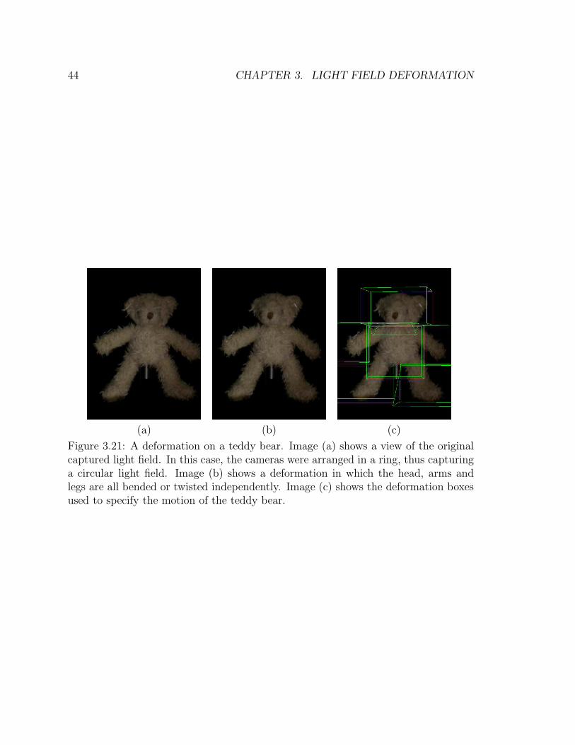
44 CHAPTER 3. LIGHT FIELD DEFORMATION
(a) (b) (c)
Figure 3.21: A deformation on a teddy bear. Image (a) shows a view of the originalcaptured light field. In this case, the cameras were arranged in a ring, thus capturinga circular light field. Image (b) shows a deformation in which the head, arms andlegs are all bended or twisted independently. Image (c) shows the deformation boxesused to specify the motion of the teddy bear.
Chapter 4
LightShop: A System for
Manipulating Light Fields
4.1 Introduction
The first half of this dissertation introduced light field deformation. This tool, like
those found in the literature, operates in a stand-alone application. In comparison,
image manipulation applications, like Adobe Photoshop, allow a user to use and
combine multiple tools. The ability to combine tools enables creative manipulation
of images.
The second contribution of this dissertation is a system that provides a user with
a mechanism to use and combine multiple tools for manipulating light fields. We
call this system LightShop. A system that operates on multiple light fields faces two
key challenges. First, operations can manipulate light fields in a variety of ways, so
specifying an operation must be designed carefully. For example, some operations are
sum over multiple pixels in each image (like focusing), or shift pixels across images
(like deformation). Second, light fields are captured and parameterized differently,
so one must design the system so that operations are independent of the light field
representation.
45

46CHAPTER 4. LIGHTSHOP: A SYSTEM FOR MANIPULATING LIGHT FIELDS
Keeping these challenges in mind, we designed LightShop with the following goals:
1. Light field operations must be specified independent of the representation.
2. The system must be extendable to incorporate new operations.
3. The system must be amenable to graphics hardware.
The first design goal addresses the problem of multiple light field parameterizations.
The second goal addresses the problem of specifying operations and combining them.
The third goal enables interactive manipulation and editing. This also enables light
fields to be easily integrated into video games.
Given these design goals, what are common operations that should be incorporated
into LightShop? Table 4.1 lists five common operations on light fields and their
applications. Ray transforms were demonstrated in the first half of this thesis for
light field deformation. Compositing light fields is demonstrated in an application,
called “pop-up light fields,” to create ghost-free renderings from light fields. The idea
is to segment a light field into multiple two-plane parameterizations (e.g. layers),
where each ST-plane serves as a local geometric proxy to that part of the scene. The
final image is rendered by compositing the samples from each layer of the light field.
The third class of operations are the arithmetic operations on colors sampled from
light fields. This has a use in relighting applications where several light fields of an
object are captured under varying illumination. By taking linear combinations of
samples from these light fields, relighting can be simulated. The fourth operation is
focusing within a light field. Instead of creating a virtual view from a pinhole camera,
one can simulate a camera with a finite-depth-of-field by summing over sampled colors
in the light field. Researchers have demonstrate its use in seeing behind occluders and
noise reduction. The final operation is perhaps the most fundamental: synthesizing
a novel view. This involves sampling and interpolating from data in a light field to
create an image from a novel viewpoint.
Given our design goals and a list of common operations on light fields, we can now
introduce the system. To begin, we describe our conceptual model for manipulating
and combining light fields. This conceptual model will drive LightShop’s entire design.

4.2. LIGHTSHOP’S CONCEPTUAL MODEL 47
Operation Applicationray transformation light field deformation [COSL05, ZWGS02]compositing pop-up light fields [SS04]arithmetic face relighting [DHT+00]focusing synthetic aperture photography [VWJL04, IMG00, LH96]sampling novel view interpolation [LH96, GGSC96, BBM+01]
Table 4.1: Common light field operations found in the literature.
4.2 LightShop’s Conceptual Model
What does it mean to manipulate and combine light fields? To answer this question,
we borrow from current modeling packages for mesh-based geometry. In particular,
we study Pixar’s RenderMan [Ups92] and OpenGL [BSW+05]. Both software pack-
ages are designed for modeling and manipulating 3D objects. We characterize their
conceptual model as one that models a scene containing multiple objects, manipulates
these objects, and renders an output image based on the modified scene. We then
adapt this conceptual model for manipulating light fields.
In RenderMan, functions are exported to the user through the RenderMan Inter-
face. These functions modify internal state that represents the scene and rendering
contexts. Some functions enable the definition of polygons, surfaces, lights and shad-
ing properties: RiPolygon, RiSurface, RiLightSource, .... These functions are
part of the modeling process. Other functions modify previously defined objects:
RiDeformation, RiSolidBegin, .... These functions are part of the manipulation
process. Finally, after a scene is modeled and modified it is rendered by the system.
In RenderMan this rendering process is hidden from the user.
OpenGL also maintains similar internal state and exports a set of functions to
model and manipulate the scene. However, instead of hiding the rendering process,
OpenGL exposes two steps of the rendering pipeline to enable more control. The
vertex shader enables a user to manipulate vertex information. The fragment shader
allows for pixel-processing before frame-buffer operations. In other words, the frag-
ment shader is a mechanism for the user to specify how an image is rendered from
the scene.

48CHAPTER 4. LIGHTSHOP: A SYSTEM FOR MANIPULATING LIGHT FIELDS
Since both RenderMan and OpenGL are well-known modeling packages, we design
LightShop with a similar 3-part conceptual model: model, manipulate, and render.
For modeling a scene, LightShop exports functions for inserting two primitive types in
a scene: light fields and viewing cameras. Appendix C lists the associated functions.
Once a scene is composed, to manipulate it a user must specify operations on light
fields. Recalling our design goals, these operation must be specified in a way that
is independent of the light field representation, easily extendable, and amenable to
graphics hardware.
The key insight to our design is that an operation on a light field can be realized
by manipulating the viewing rays from the rendering camera. This is best explained
by an example. Recall from Chapter 3 on deformation that rendering an image of
a deformed light field can be performed in two ways: 1) transform all rays of the
light field and interpolate a novel view or 2) apply the inverse ray-transform on
all view-rays, and sample from the original light field. In the second approach, by
manipulating the view-rays we can render deformed light fields. Figure 4.1 illustrates
warping view-rays to simulate deformation. It turns out that all operations listed in
Table 4.1 can be realized by manipulating view-rays in a straight-forward manner.
warp
camera light field
Figure 4.1: Warping view rays to simulate deformation. The rays emanating fromthe camera are transformed before sampling from the light field. This can simulatethe effect of deforming the original light field.
This approach has three advantages over directly manipulating the light field.
First, specifying an operation is in terms of the view-rays, which is independent of
the parameterizations of the light field and optimized for changing only those rays
4.3. EXAMPLE: FOCUSING WITHIN A LIGHT FIELD 49
needed for rendering a 2D image. Second, these view-ray operations can be combined,
one after another. For example, one can first warp a view-ray, then sample from a
light field, then composite it with the color from another light field. In fact, these
operations are represented as functions in a language. We call a set of operations
a ray-shading program. This is similar to Ken Perlin’s Pixel Stream Editor [Per85].
The third advantage is that this language can be directly mapped to the fragment
shader, so manipulating view-rays is amenable to graphics hardware. In fact, we the
implement the ray-shading program as a fragment-shading program. The graphics
rendering pipeline executes this program for every pixel, rendering an output image.
In summary, LightShop uses a conceptual model of 1) modeling a scene, 2) ma-
nipulating that scene and 3) rendering it to an output image. Modeling is performed
by calling on LightShop’s modeling API. The scene is both manipulated and ren-
dered through the ray-shading program. The ray-shading program is a user-written
program that specifies exactly how a view-ray should interact with light fields in the
scene. The program is executed per output pixel and returns an RGBA color for that
pixel. To demonstrate how a light field is manipulated, we present an example where
render an image with shallow depth-of-field from a light field.
4.3 Example: Focusing within a Light Field
We now show an example that illustrates how a light field may be manipulated. Our
example is creating an image focused at particular depth in the light field. Objects
(represented by the light field) at the focused depth will be sharp, objects off this
depth will be blurred. Figure 4.2 briefly summarizes how focusing occurs. Focusing
is discussed in more detail in the graphics [LCV+04, WJV+05, IMG00, LH96] and
vision [VWJL04] literature.
Assume during the modeling phase a scene is created containing a single light
field and a single camera1. To manipulate the light field, a user writes a ray-shading
program that describes how view-rays are manipulated as they travel through the
light field. Figure 4.3 illustrates the ray-shading program for creating an image with
1Recall that a scene is modeled by LightShop’s modeling API, described in Appendix C.

50CHAPTER 4. LIGHTSHOP: A SYSTEM FOR MANIPULATING LIGHT FIELDS
image plane focal planelens
Figure 4.2: Focusing through a single lens. The radiance contributing to a singleimage pixel is a summation of light emitted from a point on the focal plane throughthe lens aperture. More specifically, the radiant exitance/emittance from a point onthe focal plane is integrated as the irradiance on a image pixel. The radiant exitance ofpoints off the focal plane is spread across multiple pixels (e.g. this point is “blurred”).
a shallow depth-of-field. The ray-shading program takes as input a 2D xy pixel
location. It returns an RGBA color for this pixel location. The key component is
the use of two for-loops and the summation operator to simulate light aggregation
at the pixel location. To sample from the light field, the function, LiSampleLF is
called. It takes a light field index and a ray, and returns a color sampled along that
ray direction. Appendix C contains more details about this function, LiSampleLF.
The other operations listed in Table 4.1 are implemented as easily as focusing.
They are discussed in Appendix C. Now that we have discussed the conceptual
model behind LightShop and shown how to implement operations, we present the
LightShop design in the following section.
4.4 LightShop’s Design
Figure 4.4 illustrates the overall design of LightShop. The system is designed to follow
the model, manipulate, render conceptual model. It takes two inputs. The first is a
series of function calls to model a scene. The second input is a ray-shading program
that describes how a pixel should be colored, given the scene (e.g. the manipulating

4.4. LIGHTSHOP’S DESIGN 51
LtColor main(LtVec2 pixelLocation) {
LtColor sum = LtVec4(0,0,0,0);
for(i=0; i < 1.0; i += 0.1) {
for(j = 0; j < 1.0; j += 0.1) {
LtRay ray = LiGetRay(0, pixelLocation, LtVec2(i,j));
LtColor col = LiSampleLF(0,ray);
sum += col;
}
}
return sum;
}
Figure 4.3: Example ray-shading program for focusing. The core functionality thatenables focusing is that two for-loops and a summation are used to simulate theaggregation at a pixel location, over the lens aperture. The two LightShop ray-shadingfunctions, LiGetRay and LiSampleLF are discussed in more detail in Appendix C.
and rendering component). The output is a 2D image.
Following the arrows in Figure 4.4, the input modeling calls are evaluated by the
modeler, which creates an internal representation of the scene. This scene repre-
sentation is passed to the renderer, which takes the input ray-shading program and
executes it over every output pixel location to produce a 2D image. To manipulate
and combine light fields, a user modifies the ray-shading program. As the ray-shading
program executes, it accesses the scene to retrieve data from the light fields. Recalling
our three design goals, first note that the ray-shading program defines operations on
rays, which is independent of the light field representation. Second, since the program
utilizes a ray-shading language, new operations can be easily defined simply by writ-
ing new expressions. Third, the job of the renderer, which executes the ray-shading
program at each ouput pixel location, can be directly mapped to a fragment shader.
This makes LightShop amenable to graphics hardware.
Note that this design is independent of any implementation. LightShop can be
thought of as a specification for manipulating and rendering light fields. In the fol-
lowing section we discuss one particular implementation of LightShop using OpenGL.
Other implementations (using DirectX, for example) are also possible.

52CHAPTER 4. LIGHTSHOP: A SYSTEM FOR MANIPULATING LIGHT FIELDS
LightShop
scene
LtColor main(LtVec2 pos) {
LtVec2 lens = LtVec2(0,0);
LtRay ray =
LiGetRay(0, pos, lens);
LtColor samp =
LiSampleLF(0, ray);
}
LtColor main(LtVec2 pos) {
LtVec2 lens = LtVec2(0,0);
LtRay ray =
LiGetRay(0, pos, lens);
LtColor samp =
LiSampleLF(0, ray);
}
modeler
renderer
LtInt camera0 = LiCamera();
LtInt lightfield0 =
LiLightField(”flower”);
A
P
I
ray-shading program
function calls
output image
Figure 4.4: Overview of LightShop. The user passes two inputs to the system. Thefirst is a series of function calls that define a scene. The second is a ray-shadingprogram denoting how a pixel should be colored, given the scene. The function callsare passed to the modeler which creates an internal representation of the scene. Thescene is outputted to LightShop’s renderer, which takes the user-defined ray-shadingprogram and executes it per pixel of the output image. During computation, theray-shading program accesses the scene. When the renderer has executed for everyoutput pixel location, the output image is constructed and outputted.
4.5 The LightShop Implementation
Recall that LightShop is composed of three parts: the modeling interface, the ray-
shading language, and the renderer. The modeling interface is implemented in C++;
the ray-shading language and the renderer leverage the OpenGL programmable ren-
dering pipeline. The goal of the system is to manipulate and render light fields. First,

4.5. THE LIGHTSHOP IMPLEMENTATION 53
we describe our light field representation.
4.5.1 Light Field Representation
All light fields are represented by a set of images, regardless of parameterization and
acquisition method. These images have a RGBA color per pixel2. The images are
concatenated together into a single file3. The file is then compressed using S3 tex-
ture compression [INH99], yielding a 4:1 compression ratio. This compressed datafile
represents the light field. The compression rate is modest, and few artifacts are
visible. However, Figure 4.5 illustrates a case where the compression artifacts are evi-
dent. Other compression techniques exist for light fields: vector-quantization [LH96],
predictive image coding [MG00], wavelet-based compression [Pe01], as well as model-
based compression [MRG03]. However, S3 texture compression is supported natively
on the graphics hardware; decompression is quick and invisible to LightShop.
All acquired data is converted to this internal representation. During the modeling
phase, when a light field is inserted into the scene, the appropriate file is loaded from
disk and stored into memory. The modeling implementation is described next.
4.5.2 LightShop’s Modeling Implementation
LightShop’s modeling interface is implemented in C++ and utilizes the OpenGL
graphics state to pass information to the ray-shading component. The programmer
uses the interface to load light fields and define cameras. When a procedure is called
to insert a light field, LightShop loads the compressed file from disk to graphics
memory in the form of a 3D texture. Similarly, when a user calls a function to insert
a camera, data structures are allocated in graphics memory as uniform variables.
Uniform variables are variables that are accessible by the fragment shader and are
fixed when rendering a primitive in OpenGL4. In this way, when the ray-shading
2Alpha is obtained using active illumination (Appendix B) or focusing (Appendix D).3For the two-plane parameterization, the images are first rectified to a common plane before being
concatenated together. The rectification is performed by taking a light field of a planar calibrationtarget [VWJL04].
4For more information on programmable graphics hardware, the reader is referred to [Ros04].
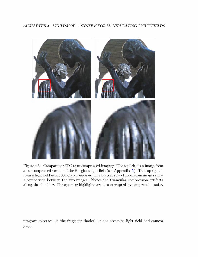
54CHAPTER 4. LIGHTSHOP: A SYSTEM FOR MANIPULATING LIGHT FIELDS
Figure 4.5: Comparing S3TC to uncompressed imagery. The top left is an image froman uncompressed version of the Burghers light field (see Appendix A). The top right isfrom a light field using S3TC compression. The bottom row of zoomed-in images showa comparison between the two images. Notice the triangular compression artifactsalong the shoulder. The specular highlights are also corrupted by compression noise.
program executes (in the fragment shader), it has access to light field and camera
data.

4.6. RESULTS USING LIGHTSHOP 55
4.5.3 LightShop’s Ray-shading Implementation
LightShop’s ray-shading language is implemented using the OpenGL Shading Lan-
guage (GLSL) [Ros04]. In other words, the ray-shading program is run through a pre-
processor which performs variable name mangling, macro substitution and for-loop
expansions to facilitate auxiliary state that LightShop needs in order to maintain a
consistent graphics environment. The preprocessed ray-shading program is now valid
GLSL code and is compiled by the graphics driver and linked into the rendering pro-
gram for execution. The details are of the implementation are discussed in Appendix
C.
Using GLSL is advantageous because it is designed for real-time rendering. This
enables LightShop to be used as an interactive editing tool or as a library for games.
Sampling from light fields is fast because GLSL takes advantage of texture memory
coherence. Additionally, bilinear interpolation from one slice is computationally free
so quadrilinear interpolation takes 4 computations as opposed to 16. A second ad-
vantage is that rendering an output image is taken care of by OpenGL. That is, the
converted ray-shading program (e.g. fragment shader) is automatically executed for
every output pixel and stored in the frame buffer. In fact, the LightShop’s renderer
implementation is exactly OpenGL’s rendering pipeline.
Given this implementation, we now show results of using LightShop in digital
photography and interactive games.
4.6 Results Using LightShop
The following results show applications of LightShop to digital photography and in-
teractive games. All light fields and their properties are enumerated in Appendix A.
Animation results are found on the website at
http://graphics.stanford.edu/papers/bchen_thesis .

56CHAPTER 4. LIGHTSHOP: A SYSTEM FOR MANIPULATING LIGHT FIELDS
4.6.1 Digital Photography
In this first demonstration, LightShop is used in two digital photography applications:
1) composing multiple light fields, similar to Photoshop for images, and 2) performing
novel post-focusing for sports photography.
Composing Scenes
LightShop can be used as a compositing tool for light fields, the 4D analogy to
image compositing with Adobe Photoshop. As a demonstration, LightShop is used
to composite light fields of several actors into a light field of a wedding couple. Figure
4.6 shows one image from this wedding light field. This light field was captured using
a hand-held light field camera [NLB+05].
Figure 4.6: An image from a light field of a wedding couple.
Figure 4.7 shows images from three light fields of three actors. We will composite
these actors into the wedding light field. The actors are captured using the camera
array. Each actor is standing in front of a green screen to facilitate matte extraction
[SB96]. Additionally, we acquire a light field of each actor under two lighting condi-
tions: left light on and right light on. In order to acquire these multiple light fields,
the actor must stand still for about 10 seconds. The purpose of acquiring light fields
under different illumination is to enable coarse relighting. LightShop can simulate
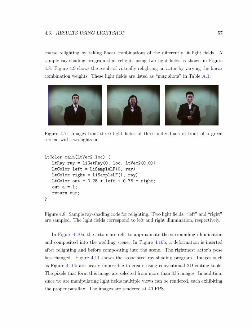
4.6. RESULTS USING LIGHTSHOP 57
coarse relighting by taking linear combinations of the differently lit light fields. A
sample ray-shading program that relights using two light fields is shown in Figure
4.8. Figure 4.9 shows the result of virtually relighting an actor by varying the linear
combination weights. These light fields are listed as “mug shots” in Table A.1.
Figure 4.7: Images from three light fields of three individuals in front of a greenscreen, with two lights on.
LtColor main(LtVec2 loc) {
LtRay ray = LiGetRay(0, loc, LtVec2(0,0))
LtColor left = LiSampleLF(0, ray)
LtColor right = LiSampleLF(1, ray)
LtColor out = 0.25 * left + 0.75 * right;
out.a = 1;
return out;
}
Figure 4.8: Sample ray-shading code for relighting. Two light fields, “left” and “right”are sampled. The light fields correspond to left and right illumination, respectively.
In Figure 4.10a, the actors are relit to approximate the surrounding illumination
and composited into the wedding scene. In Figure 4.10b, a deformation is inserted
after relighting and before compositing into the scene. The rightmost actor’s pose
has changed. Figure 4.11 shows the associated ray-shading program. Images such
as Figure 4.10b are nearly impossible to create using conventional 2D editing tools.
The pixels that form this image are selected from more than 436 images. In addition,
since we are manipulating light fields multiple views can be rendered, each exhibiting
the proper parallax. The images are rendered at 40 FPS.

58CHAPTER 4. LIGHTSHOP: A SYSTEM FOR MANIPULATING LIGHT FIELDS
Figure 4.9: Virtually relighting an individual by taking linear combinations of colorsof rays sampled from two light fields. The left- and right-most images are from theoriginal light fields, lit from the left and right, respectively. The second image issampled from a light field that takes 0.66 of the left light field and 0.33 of the rightone. The third image uses the ratios 0.33 and 0.66 for the left and right light fields,respectively. Because the illumination is at only two positions, simulating a smoothlymoving light source by blending will cause the shadows to incorrectly hop around.
(a) (b)
Figure 4.10: (a) An image from the composite light field. To approximate the illumi-nation conditions in the wedding light field, we take linear combinations of the lightfields of a given individual under different lighting conditions. The illumination doesnot match well because the lighting conditions were too sparse. (b) An image fromthe composite light field where we have turned a couple individuals’ heads.
Manipulating Focus
The next demonstration uses LightShop as a post-focusing tool. However, unlike
conventional focusing (see Section 4.3), which has a single plane of focus, LightShop

4.6. RESULTS USING LIGHTSHOP 59
LtColor main(LtVec2 loc) {
LtRay ray = LiGetRay(0, loc, LtVec2(0,0))
// deform light fields
...
// relight light fields
...
// composite light fields together
LtColor out = LiOver(woman, wedding);
out = LiOver(right_man, out);
out = LiOver(left_man, out);
return out;
}
Figure 4.11: Ray-shading code for compositing the wedding scene.
allows a user to create an image with multiple planes of focus. This feature is useful
in sports photography, where areas of interest may occur at multiple depths. A sports
photographer would then want to focus only on these depths. For example, Figure
4.12 shows one image from a light field captured of several Stanford swimmers. We
will show how to use LightShop to create an image where different swimmers are in
focus.
Figure 4.12: One image from the swimmers light field. Notice that are multiple planesof interest, corresponding to each swimmer.

60CHAPTER 4. LIGHTSHOP: A SYSTEM FOR MANIPULATING LIGHT FIELDS
The key idea is to combine the focusing and compositing operator using LightShop.
We focus on different depths of the light field and composite these focused images
together. In order to independently blur different depths of the light field, we segment
it into layers. Recall from Section 3.6 that a layer is a subset of the original light
field. In this case, instead of using projectors for light field segmentation, we use
focus. Appendix D describes this focus-based segmentation technique in more detail.
Treated as a black box, the algorithm takes a light field as input, and outputs separate
layers (e.g. light fields).
Once the light field has been segmented into layers, a separate “focused image”
can be computed from each layer. Each layer’s sharpness is specified by its own
camera and focal depth. In other words, if the light field is segmented into 3 layers,
the user defines 3 cameras in the scene, one for each layer. The focal properties of
each camera determine how light in the layer is integrated for a single pixel. Figure
4.13 illustrates how the integration occurs for a single pixel, through multiple layers.
One important aspect of this focusing process is the ordering in which compositing
rays and focusing (e.g. integration) occurs. If one were to integrate rays from each
layer of the light field and composite afterwards, this would produce an incorrect
result. The physically correct result is to first composite individual rays (i.e. the
black ray segments in Figure 4.13), then integrate the composited rays together. In
addition, since each layer is a light field (and not an image), the refraction of the rays
enables defocusing to see through occluders and around corners. This is impossible to
perform correctly if the layers are only 2D images. Figure 4.14 shows the ray-shading
program that accomplishes this compositing and focusing result.
In summary, in order to create a multi-focal plane image of the Stanford swimmers,
first segment the light field into layers, one for each swimmer. Appendix D describes
how the layers can be extracted from the swimmers light field. Second, insert each
layer into the scene. For each layer, insert a lens camera. The cameras have the
same attributes (i.e. image plane, lens aperture, lens position, etc.) except for the
focal distance5. The focal distance controls the amount of blurring for that layer.
5If the four cameras had different poses and had pinhole apertures, one could also use LightShopto construct multi-perspective images like cross-slit images, panoramas, or general linear cameras[YM04].
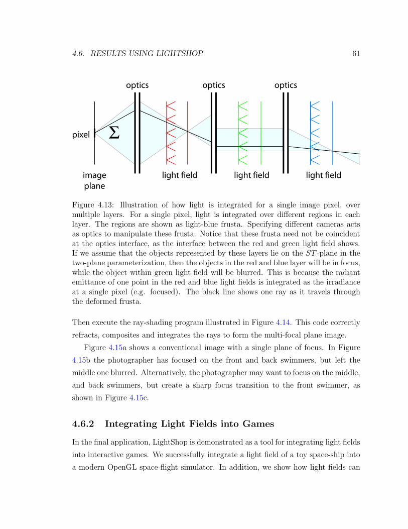
4.6. RESULTS USING LIGHTSHOP 61
light field light fieldlight field
pixel
image
plane
optics optics optics
Σ
Figure 4.13: Illustration of how light is integrated for a single image pixel, overmultiple layers. For a single pixel, light is integrated over different regions in eachlayer. The regions are shown as light-blue frusta. Specifying different cameras actsas optics to manipulate these frusta. Notice that these frusta need not be coincidentat the optics interface, as the interface between the red and green light field shows.If we assume that the objects represented by these layers lie on the ST -plane in thetwo-plane parameterization, then the objects in the red and blue layer will be in focus,while the object within green light field will be blurred. This is because the radiantemittance of one point in the red and blue light fields is integrated as the irradianceat a single pixel (e.g. focused). The black line shows one ray as it travels throughthe deformed frusta.
Then execute the ray-shading program illustrated in Figure 4.14. This code correctly
refracts, composites and integrates the rays to form the multi-focal plane image.
Figure 4.15a shows a conventional image with a single plane of focus. In Figure
4.15b the photographer has focused on the front and back swimmers, but left the
middle one blurred. Alternatively, the photographer may want to focus on the middle,
and back swimmers, but create a sharp focus transition to the front swimmer, as
shown in Figure 4.15c.
4.6.2 Integrating Light Fields into Games
In the final application, LightShop is demonstrated as a tool for integrating light fields
into interactive games. We successfully integrate a light field of a toy space-ship into
a modern OpenGL space-flight simulator. In addition, we show how light fields can

62CHAPTER 4. LIGHTSHOP: A SYSTEM FOR MANIPULATING LIGHT FIELDS
LtColor main(LtVec2 currentPixel) {
LtColor finalColor = LtVec4(0,0,0,0);
LtColor sum = LtVec4(0,0,0,0);
// iterate over the lens aperture
for(float x=0.0;x<1.0;x+=1.0/16) {
for(float y=0.0;y<1.0;y+=1.0/16) {
LtColor composite_sample = LtVec4(0,0,0,0);
// iterate over the 3 layers in the scene
for(float i = 0; i < 3; i++) {
LiVec2 lensSample = LtVec2(x,y);
// form a ray from camera i’s optical properties
LtRay ray = LiGetRay(i, currentPixel, lensSample);
// sample from light field i
LtVec4 sample = LiSampleLF(i, ray);
// composite the ray colors
composite_sample = LiOver(sample, composite_sample);
}
// sum over the aperture
sum += composite_sample;
}
}
return finalColor;
}
Figure 4.14: Ray-shading code for multi-plane focusing. The first 2 for-loops iterateover the lens aperture. The inner for-loop iterates over the light field field layers. Foreach layer, the ray is transformed according to the optics of the associated camera.Then the appropriate light field is sampled, using this ray. The returned color valueis composited with colors along previous ray segments. The final composited color isthen summed with other rays in the aperture to produce the focusing effect.

4.6. RESULTS USING LIGHTSHOP 63
(a) (b) (c)
Figure 4.15: (a) Conventional focusing in a light field. The front swimmer lies on thefocal plane. (b) A multi-focal plane image where the front and back swimmers arebrought into focus for emphasis. The middle swimmer and the crowd are defocused.(c) The front swimmer is defocused, but a large depth of field exists over the depthsof the middle and back swimmer. There is a sharp transition in focus between thefront and mid swimmers, but the photograph still has a pleasing result.
be hacked, using LightShop, for producing refraction and shadowing effects. These
effects are described in Appendix E.
Light Fields in Vega Strike
Because LightShop is implemented in OpenGL and GLSL, this makes it easy to
integrate it into interactive games. Game programmers that utilize the programmable
vertex and fragment shaders can use LightShop’s functions to access light fields like
any other texture. The vertex shader needs only to define a quad spanning the
projected area of the light field and the fragment shader executes the LightShop’s
ray-shading program to color the quad. From the game programmer’s point of view,
LightShop provides an interface for a “3D billboard” [MBGN98, AMH02] 6.
To demonstrate LightShop’s use in interactive games, it is integrated into Vega
Strike, an open-source OpenGL-based space-ship game [Hor06]. Vega Strike is a
popular spaceflight simulator with 1.3 million downloads since its inception in 2001. It
is a medium-sized open source project with approximately 100,000 lines of code. The
6The billboard appears 3D since a 3D object appears to be inside it, but in fact the light fieldrepresentation is in general 4D.

64CHAPTER 4. LIGHTSHOP: A SYSTEM FOR MANIPULATING LIGHT FIELDS
game is well supported by the community, with multiple user-contributed modules
including Privateer, and Wing Commander. Figures 4.16 shows some screenshots of
the game.
The light field that we wish to insert into Vega Strike represents a toy ship. The
acquired light field is uniformly sampled [CLF98] around the toy ship. Figure 4.17
shows a view from this light field.
Figure 4.16: Images from Vega Strike.
In VegaStrike, each model has multiple meshes defining its geometry. Each mesh in
turn has one associated 2D texture map. In the game loop, when a mesh is scheduled
to be drawn at a particular location, the appropriate MODELWVIEW matrix is loaded
into OpenGL and the associated texture is made active. The mesh vertices are then
passed to OpenGL, along with the associated texture coordinates.
To integrate LightShop into VegaStrike, the game programmer defines a Tex-
ture4D sub-class that references the light field data. The mesh for a light field object
is simply a quadrilateral spanning [-1, 1] x [-1, 1] x [-1, -1] in x, y, and z in normalized
device coordinates. The vertex shader takes this quadrilateral and maps it to the cor-
rect screen coordinates, depending on the location of the view camera and the light
field. The game programmer writes a simple ray-shading program (e.g. fragment
program) that samples from the light field. This fragment shader is activated when
the light field is ready to be drawn. Figure 4.18, shows the light fields of the toy ships
integrated into the game.

4.7. SUMMARY 65
Figure 4.17: Image from a light field of a toy space ship.
The significance of this application is that through the use of LightShop, light
fields can be integrated into the standard graphics pipeline. This means that one
can take real-world objects and place them into games or other graphics applications.
Another possibility is to use light fields from pre-rendered images of complex scenes.
This effectively caches the images of a traditional 3D object, and LightShop is used to
interactively render it. This level of facility in integrating light fields into interactive
applications is unprecedented. Hopefully it will encourage the use of such image-based
models in interactive games.
4.7 Summary
In summary, the second contribution of this thesis is LightShop, a system for gen-
eral manipulation and rendering of light fields. It borrows from traditional modeling
packages by using the model, manipulate, render conceptual model. The modeling
component is represented by an API. Manipulating and rendering a light field is rep-
resented by manipulating view-rays as they emit from the virtual viewpoint. These

66CHAPTER 4. LIGHTSHOP: A SYSTEM FOR MANIPULATING LIGHT FIELDS
Figure 4.18: In-game screen captures of the light fields of the toy ships in Vega Strike.The game runs in real-time (30+ fps). In the top-left, the protagonist approachesan unidentified space-craft. Notice that the light field is integrated seamlessly intothe surrounded 3D graphics. The top-right shows a closer view of the ship. Detailedgeometry can be seen. Bottom-left shows an out-of-cockpit view where the protagonisthas attacked the ship. The ship’s shields light up around the light field. In thebottom-right the ship light field makes a pass by the cockpit. A particle system forthe thrusters has been rendered with the light field.
manipulations are encapsulated in a ray-shading language that allows for novel defi-
nitions of operations and combining existing ones.
The system satisfies our initial design goals for building a light field manipula-
tion system. The conceptual model of manipulating view-rays instead of light fields
allows the user to abstract away the actual light field representation. The use of
a ray-shading language enables for easily extending the system to new operations
and combinations of operations. Finally, by mapping the ray-shading language to a
fragment shader, the system is amenable to graphics hardware.

4.7. SUMMARY 67
We show several compelling examples using LightShop in digital photography and
interactive games. These demonstrations illustrate that LightShop can not only oper-
ate on a variety of light fields, but allows a user to creatively combine and manipulate
them. It is our hope that LightShop can serve as a core component in any light field
manipulation application. This thesis illustrates one step towards that direction.

68CHAPTER 4. LIGHTSHOP: A SYSTEM FOR MANIPULATING LIGHT FIELDS

Chapter 5
Conclusions and Future Work
This thesis presents two contributions towards light field manipulation. The first is
an interactive technique for deforming a light field. We discuss the two key chal-
lenges to deformation: specifying a ray-transformation and maintaining consistent
illumination. Our solutions are a modified free-form deformation and coaxial light
fields. The second is a system, LightShop, that enables for general manipulation of
a light field. We design the system to abstract away the light field parameterization,
be easily extendable, and be amenable to graphics hardware. The system is designed
having three-stages: model, manipulate, and render. We have demonstrated that
deformations and LightShop have applications in photo-realistic animation, digital
photography, and interactive games.
Above are just a few domains that could benefit from a system like LightShop.
Other potential domains include opthalmology, surgical simulation, or rapid proto-
typing of scenes. In opthalmology, one important problem is the synthesis of scenes,
as seen through human optical systems, for the analysis of corneal aberrations or
diseases [Bar04]. LightShop can use Shack-Hartmann wavefront data to refract view-
rays, and sample from light fields of real scenes. The images rendered using Light-
Shop would contain optical aberrations consistent with human eye characteristics and
also be rendered from imagery representing real scenes. Because LightShop allows a
user to arbitrarily manipulate rays, there is a potential for designing optical systems
to correct for such aberrations. In surgical simulation, LightShop can be used to
69

70 CHAPTER 5. CONCLUSIONS AND FUTURE WORK
simulate dynamic organ behavior by the use of light field deformation. The visual
feedback of a realistic deforming organ may be useful for training purposes. In rapid-
prototyping of scenes, film directors or game designers may want to quickly compose a
photo-realistic scene, for pre-visualization purposes. Fundamentally, LightShop offers
a simple mechanism for composing realistic scenes.
LightShop could be extended in a number of ways. First, one can find more
uses for LightShop itself. For example, light field segmentation (either using active
illumination or focus) could be better incorporated into the editing pipeline. Another
novel use of LightShop is in combining multi-perspective imaging (i.e. panoramas)
with focusing. One could produce panoramas that contain spatially-varying focus
properties. This might be useful in blurring unwanted objects in street panoramas.
A third use of LightShop is to modify a 3D modeling tool, like 3D Studio Max, to
output function calls to drive LightShop. In this sense, LightShop acts as a light field
renderer plugin for the modeling tool.
Other improvements extend LightShop’s architecture. For example, in addition
to RGBA per ray, one could incorporate depth, normal, or time as additional data.
This would allow for more creative operations like painting, or new datasets like
time-varying light fields. These extensions are incremental steps toward the ultimate
editing tool: manipulation of reflectance fields. Since reflectance fields represent the
exitant light field as function of incident lighting (it is 8 dimensional), it is a more
comprehensive representation than a light field. In time, as data-acquisition becomes
easier and compression techniques improve, one can imagine extending LightShop to
ReflectShop, a general editing tool for reflectance fields. ReflectShop would enable
not only changes in the shape of captured objects, but also changes in incident illumi-
nation. A scene composited in ReflectShop would encapsulate correct global illumi-
nation, i.e. shadows, inter-reflection, scattering, etc. This has the potential to allow
directors to completely synthesize realistic actors, immerse gamers in a completely
real environment, or enable doctors to train on photo-realistic simulation imagery.
Hopefully, such editing tools will increase the use of image-based models in computer
graphics.

Appendix A
Table of Light Fields and their
Sizes
LF Resolution Width Height Size Acquisition Fig.
Buddha 128 x 128 x 32 x 32 4 RU 4 RU 16 ray-tracer C.7Burghers 256 x 256 x 16 x 16 37 37 10 LF camera 4.5fish 320 x 240 x 180 360◦ 0 13 ray-tracer 3.20flower 256 x 256 x 16 x 16 550 80 16 gantry C.7giraffe 256 x 256 x 16 x 16 550 80 16 gantry E.2glass ball (x2) 256 x 256 x 32 x 32 2 RU 2 RU 128 ray-tracer E.1highlight 256 x 256 x 32 x 32 2 RU 2 RU 64 ray-tracer C.8swimmers 292 x 292 x 16 x 16 37 37 10 LF camera 4.12ship 256 x 256 x 31 x 61 360◦ 124◦ 130 sph. gantry 4.17teddy bear 240 x 320 x 180 360◦ 0 13 sph. gantry 3.21toy warrior 480 x 640 x 360 360◦ 0 52 turntable 3.1twisted heads 512 x 512 x 12 x 5 1770 600 15 camera array C.5mug shots 512 x 512 x 12 x 5 1770 600 15 camera array 4.7wedding 292 x 292 x 16 x 16 37 37 10 LF camera 4.6
Table A.1: Light fields, their sizes (in MB), and acquisition methods. The Widthand Height denote maximum distance between cameras horizontally and vertically, inmm. When the light field uses a sphere-plane parameterization, “sph. gantry,” widthand height are specified in terms of degrees for θ and φ. “RU” stands for renderingunits, which is in the coordinate system of the renderer. The “turntable” acquisition isacquired by placing the toy on a mechanical turntable and taking successive snapshotswhile rotating the table.
71

72 APPENDIX A. TABLE OF LIGHT FIELDS AND THEIR SIZES

Appendix B
Projector-based Light Field
Segmentation
In this appendix, we describe a technique to segment a light field into layers, using
projector illumination. The definition of a layer is described in Section 3.6. To
motivate the use of projectors to segment a light field into layers, consider the teddy
bear shown in Figure 3.18. Suppose, before capturing a coaxial light field, we paint
the bear. We paint his head red, his body blue, his left arm green, etc. Now, when
capturing a light field of the painted teddy bear, the color of each pixel in this dataset
denotes the layer in which that pixel belongs. For example, all reddish pixels in the
light field correspond to rays which are incident to the teddy bear’s head. This
is one solution for segmenting a light field into layers: paint the individual regions
then acquired this colored light field. Unfortunately, painting the object destroys the
geometry and the appearance of the object. In other words, if we first paint the
object and acquire a colored light field, then we cannot capture the object with its
original appearance. If we first acquire a coaxial light field and then a colored light
field, then the geometry will change between acquisitions from applying the paint.
For this reason, we use projectors to effectively “paint” the object. In other words,
the image that is loaded into the projectors will color different regions of the object.
This solution preserves the object’s geometry. Afterwards, the projectors can be
turned off, and a coaxial light field can be captured for light field deformation. The
73

74 APPENDIX B. PROJECTOR-BASED LIGHT FIELD SEGMENTATION
coaxial light field is then segmented into layers (e.g. light fields) by using the color
information from the colored light field. For example, to segment the head layer from
the coaxial light field, we examine all red-colored pixels in the colored light field and
use their locations to copy from the coaxial light field to the head layer.
Figure B.1 illustrates the acquisition setup using the Stanford Spherical Gantry
[Lev04b]. Two projectors throw colors onto the teddy bear. One projector illuminates
the teddy bear’s front, and the other his back. When capturing a light field with this
projector illumination, which we call a colored light field, the color of each pixel in
the light field denotes the layer.
Figure B.1: The acquisition setup for capturing light fields. The camera is attachedto the end effector of the Stanford spherical gantry and rotates in a circle aroundthe object. Two projectors (one shown above) are placed above and outside of thegantry. The two projectors display a fixed pattern onto the front and back parts ofthe teddy bear. With the fixed pattern illuminated, the camera then proceeds tocapture a colored light field of the object. After acquiring this colored light field, theprojectors are turned off and the secondary light attached to the camera is turnedon. With this new illumination, a separate, coaxial light field is captured. The colorsin the colored light field are used to segment out layers from the coaxial light field.

75
So what images are displayed on the projectors while the camera captures images?
In the case of the teddy bear, the images are color masks that coarsely segment the
bear into regions. Note the difference between a region and a layer. A region is a
physical region on the teddy bear (i.e. the head region). The corresponding layer
is a light field in which all rays are in incident to that region. Figure B.2 shows
an example mask for the front of the teddy bear. A similar mask is created for the
projector aimed at the back of the teddy bear. The images are created by hand in
an interactive process. A person sits at a computer that has two video outputs; the
video outputs are exact clones of each other. One output is shown on a standard
CRT monitor. The other output is displayed through a projector, aimed at the teddy
bear. Using a drawing program displayed on the CRT monitor, the user paints colored
regions which are displayed live onto the teddy bear, through the projector. Drawing
the images that the projector emits takes less than 10 minutes because the images
need only to segment the bear into layers, not to precisely illuminate fine geometry
like its fur. After painting these colored regions (which are projected onto the teddy
bear), a colored light field is captured under this new illumination. The middle image
in Figure B.3 is an image from the colored light field captured with this projector
illumination.
Notice in this image that within one color region there are still changes in color
due to varying albedo or non-uniform illumination brightness. To solve this problem,
we capture an additional light field, where the projectors are emitting a floodlit white
pattern. The images from this floodlit light field are used to normalize the data from
the colored light field, thus reducing non-uniformity artifacts. Normalization of each
image of the colored light field is computed by the following equation:
B′ = 256 ∗B/W (B.1)
where W is a floodlit image (8 bits per channel), B is a colored image and B ′ is
the normalized color image. Figure B.3 shows image B′ for one camera’s view of the
teddy bear light field. Notice that the union of all colored regions in the normalized
image is also a binary mask for an object’s opacity. In other words, we may use the

76 APPENDIX B. PROJECTOR-BASED LIGHT FIELD SEGMENTATION
colored regions as an alpha mask for each image. In fact this mask is directly stored
in the alpha channel for each layer.
Figure B.2: A hand-drawn color mask is displayed on the front-facing projector tophysically segment the teddy bear into colored regions. The user draws a coarse colormask. With this illumination pattern (and a corresponding back-facing pattern)turned on, a colored light field is captured.This light field is used to segment outlayers from the coaxial light field.
In summary, to segment the teddy bear light field, we use projectors to effectively
paint the bear when we acquire the data. This colored light field has the property
that the colors of each pixel denote the layer to which that pixel belongs. Then, a
separate coaxial light field is acquired. The colors in the colored light field are used
to segment the coaxial light field into layers. Each layer has alpha per pixel, which
describes an object’s opacity. The output of this algorithm is a set of layers (e.g.
light fields), each with alpha.

77
Figure B.3: Segmenting a teddy bear light field by using projector illumination. Theleft image is the bear under floodlit illumination. The middle image shows the samebear when projected with color masks. The colors designate layers for the head, torso,arms, legs and joints. Each color denotes the layer to which that pixel belongs. Onthe right is the same view after normalization. Notice that the union of the coloredregions form an alpha mask for this image. We store this information in the alphachannel. These illumination conditions are captured for each camera position in thelight field.

78 APPENDIX B. PROJECTOR-BASED LIGHT FIELD SEGMENTATION

Appendix C
The LightShop API
This appendix describes the LightShop API and implementation details. The overall
design and motivation for the system are described in Chapter 4.
C.1 Overview of the API
Recall that LightShop consists of a modeling interface, a ray-shading language and a
rendering system. The modeling interface exports a set of functions that are used to
define a scene containing light fields. The ray-shading language is used to describe
how that scene should be rendered to a 2D image, i.e. how a view-ray is shaded,
given multiple light fields in the scene. LightShop’s renderer then executes the user-
defined ray-shading program at each pixel of the output image. Each execution of the
program shades a single pixel until the entire image is rendered. Figure 4.4 illustrates
an overview of LightShop.
To use the interface, a programmer makes a series of procedure calls to setup a
scene with light fields. These include positioning light fields and defining viewing
cameras. To describe how an image is rendered from this scene, the programmer
writes a ray-shading program that describes how a view ray from a selected camera
is shaded as it interacts with the light fields. Figures C.1 and C.2 show a program
containing procedure calls to setup a scene, and a ray-shading program that dictates
how an image should be rendered.
79

80 APPENDIX C. THE LIGHTSHOP API
First we describe LightShop’s modeling interface. Then, we describe the ray-
shading language that allows the programmer to specify how a 2D image should be
rendered from the light fields in the scene.
C.2 LightShop’s Modeling Interface
In LightShop, a scene is modeled with two primitive types: cameras with a single lens1
and light fields. The programmer calls specific functions that insert these primitives
into an internal representation of the scene. Each primitive stores its own related
information: focal distance, sampling, etc. This information is called LightShop at-
tributes or attributes for short. Table C.1 shows the supported LightShop primitives,
and their associated attributes.
In LightShop, a camera with a lens (henceforth called a “lens camera” or “cam-
era”) follows the simple lens model. Figure C.3 illustrates the model. It has an image
plane, a lens plane, and a focal plane. Intuitively, light emitted from a point on the
focal plane passes through an aperture in the lens plane and is focused onto a point
on the image plane. More specifically, on the image plane is a rectangular region
defining the digital sensor or film area. The camera attributes “lower left,” “up,” and
“right” define both the image plane and the sensor area. The lens plane is parallel
to the image plane. The lens aperture is a rectangular region lying on the lens plane.
The attributes “lens center,” “lens width,” and “lens height,” define the location of
this lens aperture. The focal plane is parallel to the lens plane and image plane. Its
location is defined by the “focal distance” attribute, which is the distance between
the focal and lens plane. Since diffraction is not modeled, a pinhole camera can be
created by setting the “lens width” and “lens height” attributes to 0. As we will see in
Section C.3.3, the LiGetRay ray-shading function makes use of the camera attributes
to form a ray, given the 2D locations of the image pixel and a sample point on the
lens.
1Although LightShop could include a more complex optical system, in practice a single lensmodel suffices for many applications. When more complexity is necessary, LightShop’s ray-shadinglanguage allows for arbitrary ray refraction (see Section C.3).

C.2. LIGHTSHOP’S MODELING INTERFACE 81
// Initialize LightShop
LiBegin();
// insert the camera
LtInt camera0 = LiCamera();
// set camera0’s attributes
LtDir lowerLeft= {-1, -1, -1};
LtDir up = {0, 2, 0};
LtDir right = {2, 0, 0};
LiDir lensCenter = {1,1,1};
LiFloat focalDistance = 10.0;
LiInt xRes = 512;
LiInt yRes = 512;
LiAttributeCam(camera0, ‘‘x res’’, &xRes);
LiAttributeCam(camera0, ‘‘y res’’, &yRes);
LiAttributeCam(camera0, ‘‘lower left’’, lowerLeft);
LiAttributeCam(camera0, ‘‘up’’, up);
LiAttributeCam(camera0, ‘‘right’’, right);
LiAttributeCam(camera0, ‘‘lens center’’, lensCenter);
LiAttributeCam(camera0, ‘‘focal distance’’, focalDistance);
// insert the light field
LtColor clear = {0, 0, 0, 0};
LtMatrix translate = {1, 0, 0, 0, 0, 1, 0, 0, 0, 0, 1, 0, 0, 0, -10, 1};
LtInt lightField1 = LiLightField(‘‘lightfield.tlf’’);
LiAttributeLF(lightField1, ‘‘sampling’’, ‘‘quadralinear’’);
LiAttributeLF(lightField1, ‘‘wrapping’’, clear);
LiAttributeLF(lightField1, ‘‘transform’’, translate);
// tell LightShop to clean up
LiEnd();
Figure C.1: A simple LightShop program that models a scene containing a lens cameraand a light field.

82 APPENDIX C. THE LIGHTSHOP API
LtColor main(LtVec2 currentPixel)
{
LtColor col = LtVec4(0,0,0,0);
// convert the current pixel location to a ray based on camera 0
LtRay=LiGetRay(0, currentPixel, LtVec2(0, 0));\\
// use the ray to sample from light field 0
col = LiSampleLF(0, ray);
// return the color sampled from the light field
return col;
}
Figure C.2: A simple ray-shading program that takes the scene modeled in FigureC.1 and returns the color of a single pixel of the display image. LightShop’s rendererexecutes the program over all pixels to compute a final image.
For light fields, we approximate the continuous 4D function with discrete samples
that can be thought of as a 4D texture. Hence, light fields in LightShop have similar,
texture-like attributes: sampling method (i.e. nearest-neighbor, or quadralinear, and
wrapping behavior (i.e. repeat or clamp to a value). Nearest-neighbor sampling
simply extracts the color of the ray “nearest” to the input ray. Quadralinear sampling
[LH96] is the 4D equivalent to bilinear interpolation in 2D.
The third light field attribute, “transform”, is an optional attribute that allows the
programmer to pass implementation-specific parameters to LightShop. For example,
in the implementation described in Section 4.5, LightShop supports the two-plane pa-
rameterization of light fields. The “transform” attribute is used to pass a 4x4 matrix
that is applied to the vectors describing the UV- and ST-plane of the light field. This
allows a programmer to position a light slab by providing an appropriate transform
matrix. Other implementations may use this attribute for other applications.
Notice that LightShop does not specify a particular light field parameterization;
the attributes are invariant to this and the implementor may support various types
(i.e. UVST 2-plane, sphere-plane, circular, etc.) at her discretion.

C.2. LIGHTSHOP’S MODELING INTERFACE 83
lens_center
x
y
z
lower leftright
up lens_center
width
he
igh
tfocal distance
Figure C.3: The lens model used in LightShop. The pink, green and blue rectan-gles are the sensor area, lens aperture and focal plane, respectively. These cameraattributes are used by the LiGetRay ray-shading function, described in Section C.3.3.
C.2.1 Graphics Environment (Scene)
Given the previously defined primitives, a programmer creates a scene by calling
specific functions that modify an internal representation of the world. This internal
representation is called the graphics environment or scene, which is invisible to the
programmer and completely contained within LightShop. The graphics environment
is simply a set of cameras and a set of light fields; it is shared between the modeling
interface and the ray-shading language.

84 APPENDIX C. THE LIGHTSHOP API
C.2.2 Modeling Functions Available to the Programmer
The goal of the LightShop functions is to provide an interface between the programmer
and the graphics environment. The functions use specific data types defined by
LightShop for arguments and return values. We first define these data types, then
describe the procedures that use them. The data types are presented using a C-
like syntax as an explanatory medium. However, note that LightShop can also be
implemented in other high-level languages like Java or Python.
The name of each data type is prefixed with Lt (LightShop type). Procedures
and variables are prefixed with Li (LightShop interface).
Scalar Types
typedef long LtInt;
typedef float LtFloat;
typedef char* LtString;
typedef void LtVoid;
typedef void* LtPointer;
LightShop supports the usual data types found in C.
Vector Types
class LtVector3;
class LtVector4;
class LtMatrix3;
class LtMatrix4;
typedef LtVector3 LtPoint;
typedef LtVector3 LtDir;
typedef LtVector4 LtColor;
The Vector[34] types are generic vectors used for variables containing 3D points,
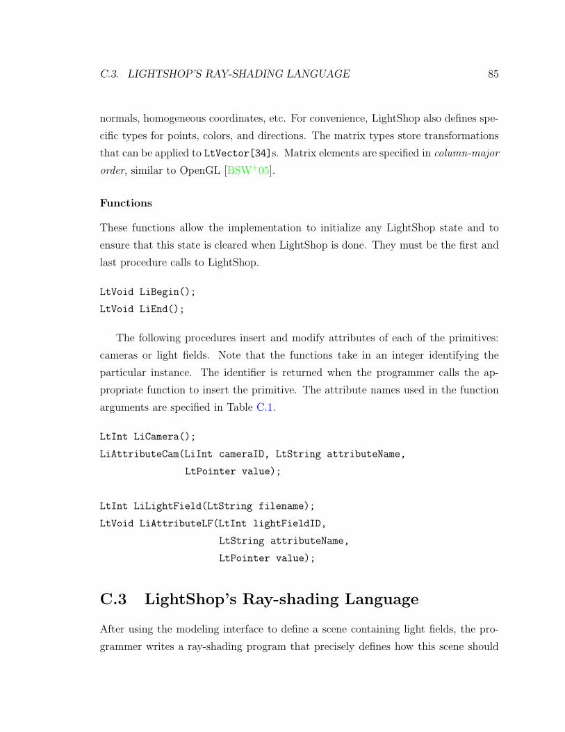
C.3. LIGHTSHOP’S RAY-SHADING LANGUAGE 85
normals, homogeneous coordinates, etc. For convenience, LightShop also defines spe-
cific types for points, colors, and directions. The matrix types store transformations
that can be applied to LtVector[34]s. Matrix elements are specified in column-major
order, similar to OpenGL [BSW+05].
Functions
These functions allow the implementation to initialize any LightShop state and to
ensure that this state is cleared when LightShop is done. They must be the first and
last procedure calls to LightShop.
LtVoid LiBegin();
LtVoid LiEnd();
The following procedures insert and modify attributes of each of the primitives:
cameras or light fields. Note that the functions take in an integer identifying the
particular instance. The identifier is returned when the programmer calls the ap-
propriate function to insert the primitive. The attribute names used in the function
arguments are specified in Table C.1.
LtInt LiCamera();
LiAttributeCam(LiInt cameraID, LtString attributeName,
LtPointer value);
LtInt LiLightField(LtString filename);
LtVoid LiAttributeLF(LtInt lightFieldID,
LtString attributeName,
LtPointer value);
C.3 LightShop’s Ray-shading Language
After using the modeling interface to define a scene containing light fields, the pro-
grammer writes a ray-shading program that precisely defines how this scene should

86 APPENDIX C. THE LIGHTSHOP API
be rendered to a 2D image. An image is created by associating a ray to each out-
put pixel, and deciding on how to shade this “view-ray”. As the view-ray travels
through the scene, its color (RGBA) or direction may change due to interaction with
light fields. This is similar to ray-tracing except that objects are represented by light
fields. LightShop’s ray-shading language allows the programmer to precisely define
how this view ray is affected by the light fields.
The ray-shading language executes in a manner similar to the Pixel Stream Editor
[Per85]. It takes as input the xy location of a pixel of the 2D image, executes the
ray-shading program at this pixel, and outputs a RGBA color. At any one pixel,
the program has access to the graphics environment (i.e. the light fields and the
cameras). It uses this environment to first form a ray from the given pixel position
and then to shade the color of this ray. The pixel color is set to the computed ray
color. LightShop’s renderer executes the same ray-shading program at each pixel
location to progressively construct the final image.
First we describe the language’s data types, then flow control, then high-level
functions available to the programmer. We use GLSL [Ros04] as the explanatory
medium for data types and procedures. It has a C-like syntax and we build func-
tionality on top of it in our implementation in Section 4.5. However, note that the
ray-shading language could be implemented in other languages like C++, HLSL, or
Cg.
C.3.1 Data Types and Scope
typedef void LtVoid;
typedef int LtInt;
typedef float LtFloat;
typedef vec2 LtVec2; // A general 2-vector
typedef vec3 LtVec3; // A general 3-vector
typedef vec4 LtVec4; // A general 4-vector
typedef mat4 LtMat4; // A general 4x4 matrix of floats

C.3. LIGHTSHOP’S RAY-SHADING LANGUAGE 87
typedef vec4 LtColor; // A RGBA color value
typedef vec3 LtPoint; // A XYZ 3D point
typedef vec3 LtDir; // A direction vector
typedef vec4 LtPlane; // A plane equation Ax+By+Cz+D=0
struct LtRay {
LtVec4 pos;
LtDir dir;
};
The ray-shading language supports the standard C data types. The LtRay type
describes a ray in 3-space. It is used for sampling from a light field to obtain a color
in that ray direction. A ray in LightShop is represented by a point on the ray (in
homogeneous coordinates) and a direction. Although a ray can be described by four
parameters, the point-direction representation facilitates ray intersection calculations.
The scope of variables is the same as in C++, i.e. local scope within the enclosing
block and global scope otherwise.
C.3.2 Flow Control
The program starts execution in the main function. The same main function executes
for every output pixel of the image. It takes as input the current pixel location and
outputs a RGBA color. It can also access the global graphics environment.
Aside from a few different token names, the LightShop ray-shading language uses
the same grammar as GLSL [Ros04]. Looping is accomplished using the same syntax
and keywords as those in C++: for, while, and do ... while. Looping allows a
programmer to map the colors of multiple rays in different light fields to a single pixel
color. One useful application is for focusing, where a single pixel color is computed
by integrating over the colors of multiple rays (see Section 4.6.1). Branches also use
the same syntax as in C++: if and if ... else. This allows the program to have

88 APPENDIX C. THE LIGHTSHOP API
per-pixel variability. Functions are defined and called in the same way as in C++.
A return type is followed by the name of the function, followed by a parameter list.
The language allows for function overloading.
C.3.3 Light Field Manipulation Functions
On top of this language, LightShop offers the standard math functions (sin, asin,
pow, etc.) and several high-level functions specifically for manipulating light fields.
The ray-utility function, LiGetRay, takes as input a 2D pixel location, a 2D po-
sition on the lens aperture and a camera primitive. It uses the camera attributes,
defined in Section C.2, to produce a ray. First, LiGetRay forms an intermediate ray
based on the pixel location and sample position on the lens. This ray is then refracted
through the lens and returned as output. The amount of refraction is based on the
simple lens model; rays emitted from one point on the image plane converge to a point
on the focal plane defined by Gaussian optics. Recall that the focal plane and other
camera attributes are specified during the modeling process, described in Section C.2.
The LightShop function is the following:
LtRay LiGetRay(LiInt cameraID, LtVec2 currentPixel,
LtVec2 lensSample)
For example, in the simple ray-shading program shown in Figure C.2, LiGetRay
returns the refracted ray that started from the current pixel location, entered the lens
center and refracted out. Section 4.3 demonstrates how focusing can be accomplished
by summing the colors of rays that enter multiple positions on the lens aperture.
Once a ray has been formed, it can be passed as input to several high-level func-
tions. These functions form a basis for a wide variety of light field manipulation
operations. Additionally, these functions can be called in combination, which allows
arbitrarily complex light field manipulations.
The following are the LightShop functions: 4D sampling, which samples a RGBA
color from a light field; compositing, which combines two RGBA colors into a single
one; and warping, which maps rays to rays.
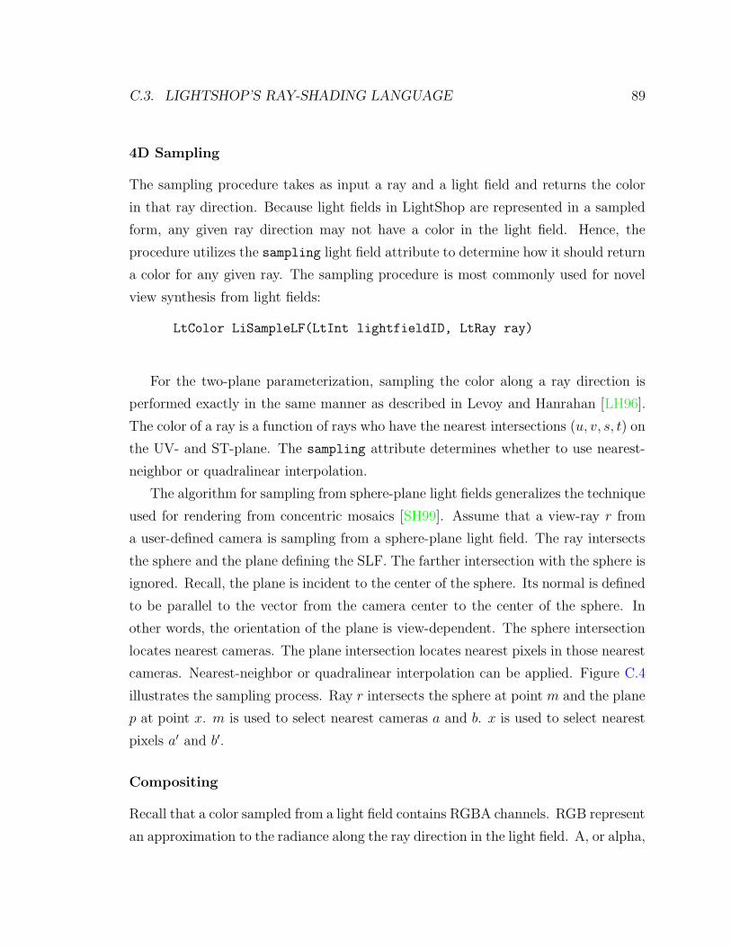
C.3. LIGHTSHOP’S RAY-SHADING LANGUAGE 89
4D Sampling
The sampling procedure takes as input a ray and a light field and returns the color
in that ray direction. Because light fields in LightShop are represented in a sampled
form, any given ray direction may not have a color in the light field. Hence, the
procedure utilizes the sampling light field attribute to determine how it should return
a color for any given ray. The sampling procedure is most commonly used for novel
view synthesis from light fields:
LtColor LiSampleLF(LtInt lightfieldID, LtRay ray)
For the two-plane parameterization, sampling the color along a ray direction is
performed exactly in the same manner as described in Levoy and Hanrahan [LH96].
The color of a ray is a function of rays who have the nearest intersections (u, v, s, t) on
the UV- and ST-plane. The sampling attribute determines whether to use nearest-
neighbor or quadralinear interpolation.
The algorithm for sampling from sphere-plane light fields generalizes the technique
used for rendering from concentric mosaics [SH99]. Assume that a view-ray r from
a user-defined camera is sampling from a sphere-plane light field. The ray intersects
the sphere and the plane defining the SLF. The farther intersection with the sphere is
ignored. Recall, the plane is incident to the center of the sphere. Its normal is defined
to be parallel to the vector from the camera center to the center of the sphere. In
other words, the orientation of the plane is view-dependent. The sphere intersection
locates nearest cameras. The plane intersection locates nearest pixels in those nearest
cameras. Nearest-neighbor or quadralinear interpolation can be applied. Figure C.4
illustrates the sampling process. Ray r intersects the sphere at point m and the plane
p at point x. m is used to select nearest cameras a and b. x is used to select nearest
pixels a′ and b′.
Compositing
Recall that a color sampled from a light field contains RGBA channels. RGB represent
an approximation to the radiance along the ray direction in the light field. A, or alpha,

90 APPENDIX C. THE LIGHTSHOP API
rx
a
b
p
ma’
b’
Figure C.4: Plan-view of rendering from a sphere-plane light field.
represents both opacity and coverage. Once a color has been sampled from a light
field, it can be composited with samples from other light fields. Using the proper
compositing operators and ordering allows a programmer to render an image of a
scene of light fields.
The compositing operator allows for all twelve of Porter and Duff’s [PD84] com-
positing operations. Similar to their formulation, LightShop assumes that the colors
in the light field are premultiplied by the alpha channel. This is useful because com-
positing equations for RGB are the same as those for alpha.
The twelve compositing operations for two RGBA colors, A and B, can be ex-
pressed as a linear combination. More specifically, to compute the composited color,
the programmer specifies weights, w1, w2 to the linear combination of A and B:
C = w1A + w2B (C.1)
For particular choices of w1 and w2, the resulting color have familiar forms, as
shown in Table C.2. The LightShop procedures in this table return a LtColor and take
in two LtColors as argument. One example is shown below for the over compositing
operator:
LtColor LiOver(LtColor A, LtColor B)

C.3. LIGHTSHOP’S RAY-SHADING LANGUAGE 91
Also, for brevity the symmetric procedure for each operation has been omitted from
the table (i.e. B over A, B in A, etc.).
Specific procedure names have been given to the common compositing operations.
The LightShop procedure for general compositing is:
LtColor LiComposite(LtFloat w1, LtColor A, LtFloat w2, LtColor B)
Warping
LightShop’s warping functions take a ray as input and return a new (i.e. warped) ray.
Ray warping is commonly used to simulate deformation of a light field [COSL05], or
refractive effects [HLCS99, YYM05].
LightShop provides two types of warps to the programmer: procedural warps and
4D table lookup. Procedural warps are commonly-used utility functions for warping
rays. These are various functions that transform points. New rays can be formed
by taking two points on the original ray, applying a transformation on them, and
forming a vector from the two new points. Some of these functions are shown below:
LtPoint LiRotateX(LtPoint v, LtFloat theta)
LtPoint LiRotateY(LtPoint v, LtFloat theta)
LtPoint LiRotateZ(LtPoint v, LtFloat theta)
LtPoint LiRotateXAboutPt(LtPoint v, LtPoint org,
LtFloat theta)
LtPoint LiRotateYAboutPt(LtPoint v, LtPoint org,
LtFloat theta)
LtPoint LiRotateZAboutPt(LtPoint v, LtPoint org,
LtFloat theta)
Figure C.5 illustrates a twisting effect that can be accomplished using LightShop’s
warping functions. Figure C.6 shows several other views of this “twisted light field”.

92 APPENDIX C. THE LIGHTSHOP API
To accomplish the twisting effect for the left individual, two points on each view
ray are selected and rotated about a vertical axis centered over the left person. The
amount of rotation is a function of the height of each of the points. The higher
a point is, the more rotation is applied. LiRotateYAboutPt is used to perform the
rotation. The warped ray is formed from the rotated points. A similar warp is defined
for twisting the right individual. To keep the left and right ray-warps from creating
discontinuities in the image, the final ray warp is a linear combination of the left and
right twists. The weight for each twist is inversely related to the ray’s proximity to
the left or right twist axes.
The warping functions that use a 4D lookup table represent the ray warp with
discrete samples. The lookup table is treated in the same way as a light field, except
that the value per ray is not an RGBA color, but a new ray. One can think of the light
field as a ray-valued one as opposed to a color-valued one. The LightShop procedure
that samples from the ray-valued light field is shown below. Notice that it returns a
ray instead of a color.
LtRay LiWarpRayLookup(LtInt lightFieldID, LtRay ray)
The lookup table is treated in the same way as a light field, except that the value
per ray is not an RGBA color, but information describing a warped ray. LightShop
represents this ray information as two 3D points on the ray. Since each point takes
3 coordinates, xyz, the warped ray needs 6 coordinates. These 6 coordinates are
stored separately in the 3 RGB channels of 2 light fields. The alpha channel of
both light fields is used to indicate if a warp exists (1) or not (0) for that particular
input ray. Using 6 coordinates to represent a ray wastes space, since a ray can
be represented by 4 coordinates. However, the extra channel is used as a flag for
when a ray warp is defined. Additionally, no extra information about the coordinate
system of the parameterization needs to be known (i.e. the plane locations for a
2-plane parameterization). By convention, it is assumed that the two light fields have
sequential identifiers, so that a ray warp lookup is performed by specifying the ray
and the light field containing the first point on the warped ray.
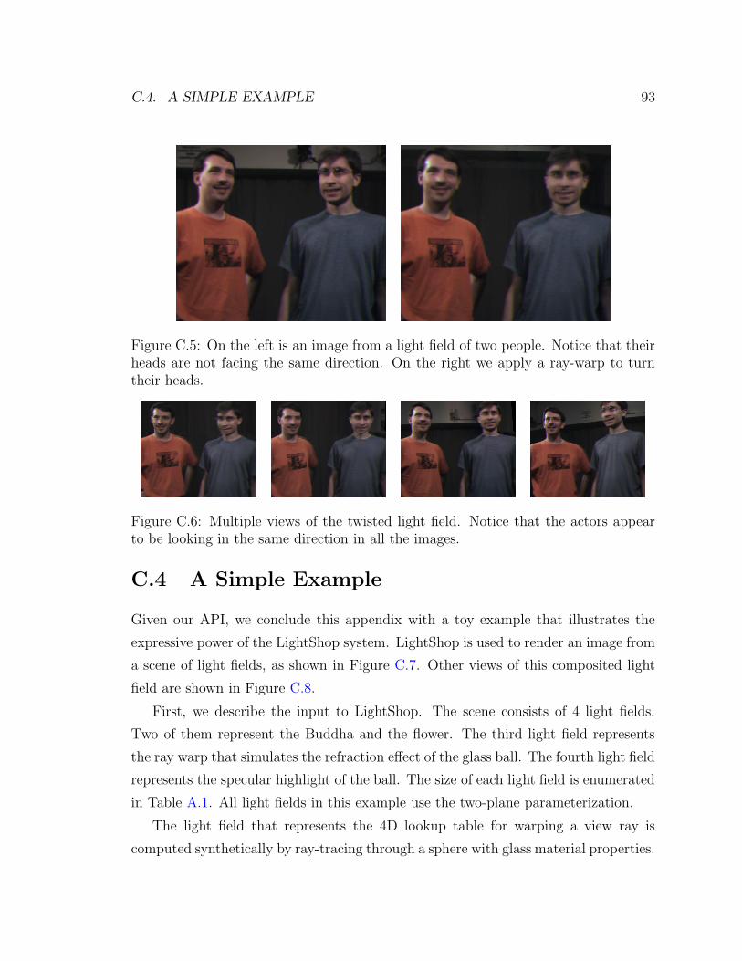
C.4. A SIMPLE EXAMPLE 93
Figure C.5: On the left is an image from a light field of two people. Notice that theirheads are not facing the same direction. On the right we apply a ray-warp to turntheir heads.
Figure C.6: Multiple views of the twisted light field. Notice that the actors appearto be looking in the same direction in all the images.
C.4 A Simple Example
Given our API, we conclude this appendix with a toy example that illustrates the
expressive power of the LightShop system. LightShop is used to render an image from
a scene of light fields, as shown in Figure C.7. Other views of this composited light
field are shown in Figure C.8.
First, we describe the input to LightShop. The scene consists of 4 light fields.
Two of them represent the Buddha and the flower. The third light field represents
the ray warp that simulates the refraction effect of the glass ball. The fourth light field
represents the specular highlight of the ball. The size of each light field is enumerated
in Table A.1. All light fields in this example use the two-plane parameterization.
The light field that represents the 4D lookup table for warping a view ray is
computed synthetically by ray-tracing through a sphere with glass material properties.

94 APPENDIX C. THE LIGHTSHOP API
More specifically, in a ray-tracing program called yafray [yaf05], we create a scene
consisting of a single sphere. We set the material properties of this sphere to mimic
refractive glass with index of refraction 1.5. Then, for 32x32 camera positions, we
ray-trace 256x256 rays into the scene containing the glass sphere. For each ray, the
ray-tracer outputs a description of the refracted ray. We store this description in the
RGBA components of the light field. This light field yields a mapping from any ray
(from the 32x32x256x256 rays) to a ray refracted through the glass ball.
Figure C.7: A rendered image from a composite light field scene.
The procedure calls that model the scene are shown in Figure C.9. Referring to
Figure C.9, the programmer first inserts a camera into the scene. It is a pinhole
camera pointed at a specific location (namely, where we will position the light fields).
The next set of procedure calls insert light fields into the scene. The integer
identifiers of each light field begin at 0 and increase sequentially (i.e. the Buddha
light field is mapped to identifier 0). Light fields 0 and 1 are typical light fields that
have RGBA as values per ray. Light field 2 is a 4D lookup table that warps rays as if
the ray had gone through a glass ball. Light field 3 is an RGBA light field containing
the specular highlight of the glass ball. Next, the programmer specifies various light
field attributes that define their position.

C.4. A SIMPLE EXAMPLE 95
Figure C.8: Novel views of the scene of composited light fields.
Once the scene has been modeled, the programmer writes a ray-shading program
that defines precisely how a 2D image is rendered from this scene. This is done by
writing a program that executes per output pixel of the image to determine the color
of each pixel, given the scene of light fields.
Figure C.10 shows the ray-shading program. We now proceed to describe each
step of the program and show its effects on the current output image.
First, we convert the current pixel location into a ray and use this ray to sample
from the Buddha light field. We set the background color to be black. Lines 5–13
produce Figure C.11.
Next, in line 17 we use the same ray to sample from the flower light field and
composite that color over the Buddha sample, which produces Figure C.12.
Now, to create the spherical refraction effect, we warp the view ray as if the ray
had gone through the glass ball. Recall that light field 2 maps an input ray to a

96 APPENDIX C. THE LIGHTSHOP API
warped ray. We use the LiWarpRayLookup procedure to acquire the warped ray. This
warped ray is then used to sample from the Buddha and the flower light field to
produce a refractive version. Figure C.13 shows the current image after lines 20–26.
Finally, in lines 44-46 we add a specular highlight to the scene by sampling from
the light field containing the ball’s specular highlight and adding this color to the
final color. This produces the final image, as shown in Figure C.7, other views are
shown in Figure C.8.

C.4. A SIMPLE EXAMPLE 97
Primitive Attribute Default Descriptionlens camera lower left [-1, -1, -1] lower left of the image plane
up [0, 2, 0] vector from the lower left to theupper left of the image plane
right [2, 0, 0] vector from the lower left to thelower right of the image plane
lens center [1, 1, 1] vector from the lower left to thecenter of the lens aperture
lens width 2 width of the lens aperturelens height 2 height of the lens aperturefocal distance 1 the perpendicular distance
between the lens plane and thefocal plane
x res 512 horizontal resolution of theoutput image
y res 512 vertical resolution of theoutput image
light field sampling quadralinear sampling method:nearest-neighbor or quadralinear
wrapping [0, 0, 0, 0] wrapping behavior when samplingoutside the light field: “clamp”,“repeat”, or a RGBA user-definedcolor
transform 4x4 identity a transformation applied to therays of the light field
Table C.1: Primitives and attributes that LightShop supports. Other image options,like bias, gain, pixel sampling rates, filter sizes, color quantization, etc., could also besupported by LightShop.
Operation w1 w2 Expression FunctionA add B 1 1 A + B +A over B 1 1− αA A + (1− αA)B LiOver
A in B αB 0 αBA LiIn
A out B 1− αB 0 (1− αB)A LiOut
A atop B αB 1− αA αBA + (1− αA)B LiAtop
A xor B 1− αB 1− αA (1− αB)A + (1− αA)B LiXor
Table C.2: Common compositing operations that have special names in LightShop.

98 APPENDIX C. THE LIGHTSHOP API
// Initialize LightShop
LiBegin();
// insert the camera
LtDir lowerLeft = {4.14, 4.00, 7.92};
LtDir up = {0.00, -8.00, 0.00};
LtDir right = {-7.99, 0.00, 0.15};
LtFloat lensWidth = 0;
LtInt camera0 = LiCamera();
LiAttributeCam(‘‘lower left’’, lowerLeft);
LiAttributeCam(‘‘up’’, up);
LiAttributeCam(‘‘right’’, right);
LiAttributeCam(‘‘lens width’’, lensWidth);
LiAttributeCam(‘‘lens height’’, lensHeight);
// insert the light fields
LtInt lightField0 = LiLightField(‘‘buddha’’);
LtInt lightField1 = LiLightField(‘‘flower’’);
LtInt lightField2 = LiLightField(‘‘glass ball’’);
LtInt lightField3 = LiLightField(‘‘highlight’’);
// set light field attributes
LtMatrix4 transform0 = {4,0,0,0,0,4,0,0,0,0,4,0,0,0,3.5,1};
LtMatrix4 transform1 = {.6,0,0,0,0,.6,0,0,0,0,.6,0,-1.25,0,4.0,1};
LtMatrix4 transform2 = {1,0,0,0,0,1,0,0,0,0,1,0,.5,0,0,1};
LiAttributeLF(lightField0, ‘‘transform’’, transform0);
LiAttributeLF(lightField1, ‘‘transform’’, transform1);
LiAttributeLF(lightField2, ‘‘transform’’, transform2);
LiAttributeLF(lightField3, ‘‘transform’’, transform2);
// tell LightShop to clean up
LiEnd();
Figure C.9: LightShop function calls that model the toy scene shown in Figure C.7.
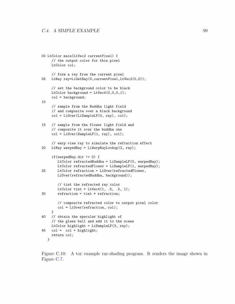
C.4. A SIMPLE EXAMPLE 99
00 LtColor main(LtVec2 currentPixel) {
// the output color for this pixel
LtColor col;
// form a ray from the current pixel
05 LtRay ray=LiGetRay(0,currentPixel,LtVec2(0,0));
// set the background color to be black
LtColor background = LtVec4(0,0,0,1);
col = background;
10
// sample from the Buddha light field
// and composite over a black background
col = LiOver(LiSampleLF(0, ray), col);
15 // sample from the flower light field and
// composite it over the buddha one
col = LiOver(SampleLF(1, ray), col);
// warp view ray to simulate the refraction effect
20 LtRay warpedRay = LiWarpRayLookup(2, ray);
if(warpedRay.dir != 0) {
LtColor refractedBuddha = LiSampleLF(0, warpedRay);
LtColor refractedFlower = LiSampleLF(1, warpedRay);
25 LtColor refraction = LiOver(refractedFlower,
LiOver(refractedBuddha, background));
// tint the refracted ray color
LtColor tint = LtVec4(1, .5, .5, 1);
30 refraction = tint * refraction;
// composite refracted color to output pixel color
col = LiOver(refraction, col);
}
40 // obtain the specular highlight of
// the glass ball and add it to the scene
LtColor highlight = LiSampleLF(3, ray);
45 col = col + highlight;
return col;
}
Figure C.10: A toy example ray-shading program. It renders the image shown inFigure C.7.

100 APPENDIX C. THE LIGHTSHOP API
Figure C.11: The image after sampling from the Buddha light field.
Figure C.12: The image after compositing the flower RGBA sample over the Buddhaone.

C.4. A SIMPLE EXAMPLE 101
Figure C.13: The image after compositing the refracted Buddha and flower lightfields. There are jaggy artifacts in the refraction due to the limited sampling rate ofthe ray warp. For simple geometric objects, this artifact can be remedied by providinga function characterizing the ray warp. For more complex objects, a higher samplingrate is necessary. LightShop can handle either solutions.

102 APPENDIX C. THE LIGHTSHOP API

Appendix D
Focus-based Light Field
Segmentation
In this appendix we describe how to segment a light into layers using focus. The
dataset we use is the swimmers light field (see Section 4.6.1 and Appendix A). Seg-
menting this dataset for a given layer is equivalent to computing an alpha matte for
each image of the light field. Thus the goal is to compute these alpha mattes.
To compute the alpha mattes for each layer, we process the layers in a front-to-
back order. For the front swimmer, an implementation of intelligent scissors [MB95b]
is used to segment it out in one of the images of the light field. Figure D.1a illus-
trates this contour and D.1b shows the binary mask. This binary mask needs to be
propagated to all images, but in this case it turns out that the front swimmer lies on
the ST plane, so the binary mask remains fixed to her silhouette in all images.
Next, a tri-map is created based on the binary mask to serve as an input to a
Bayesian matte extraction algorithm [CCSS01]. The technique is similar to the one
used by Zitnick et. al [ZKU+04]. A tri-map consists of a foreground, background,
and unknown region of the image. The foreground mask is computed by eroding the
initial binary mask (shown in Figure D.1c). The background is computed by dilating
the binary mask twice and taking the difference of the dilated masks (shown in Figure
D.1d). The unknown region lies between the foreground and background masks. This
tri-map is passed into the Bayesian matte extraction algorithm to produce the alpha
103

104 APPENDIX D. FOCUS-BASED LIGHT FIELD SEGMENTATION
matte in Figure D.1e. Figure D.1f shows the extracted front swimmer for this image.
Since this swimmer lies on the ST plane, we can use the same alpha matte to extract
her from all images.
(a) (b) (c)
(d) (e) (f)
Figure D.1: Illustration of the alpha matte extraction pipeline. The user uses intelli-gent scissors to specify a binary mask in (a). The mask is shown in (b). The mask isthen eroded by 3 pixels to form a foreground mask shown in (c). Dilating the maskby 2 and 30 pixels and taking their difference produces the background mask in (d).The output of the Bayesian matte extraction is shown in (e). A neighborhood size of4 pixels was used. (f) shows the extracted front swimmer.
For the layers belonging to the middle and back swimmer, the binary mask in a
single image will shift in the other images due to parallax. To handle this shift, we
choose a plane approximating the depth of that layer. This plane is then used to
project a binary mask in one image to all other images. In other words, the plane
acts as a geometric proxy to propagate a binary mask in one image to all other images
in the light field. How do we select the planar proxy depth? The solution is to use

105
focus.
We use LightShop to create images where we focus on different depths in the
swimmers light field. When a layer comes into focus, the corresponding depth is
recorded. Given the depth of this plane, a binary mask in one image is projected to
all other images by a homography induced by the plane [HZ00].
Now we quickly review how to compute a 3x3 homography matrix that is induced
between two cameras and a plane. Using the notation presented in Hartley and
Zisserman’s book, two cameras are defined with projection parameters, K[I|0] and
K ′[R|t]. The homography induced by a plane, nT + d = 0, is given by:
H = K ′(R− tnT/d)K−1 (D.1)
Equation D.1 correctly computes the homography for general camera positions.
However, for cameras in a two-plane parameterization, we can simplify the equation
further. For camera images from a two-plane parameterization, each camera can be
thought of as having an off-axis projection, with a common principle direction. This
means that R maps to the identity matrix and the intrinsics and extrinsics only have
a translation component that is a function of the relative camera locations in the
UV-plane. Mathematically, Equation D.1 reduces to
H = K ′(I − tnT/d)K−1 (D.2)
where K ′, K have the form of
f 0 cx
0 f cy
0 0 1
(D.3)
and t = [−cx − cy − cz]. cx, cy, and cz are the relative coordinates for the position
of the second camera. In summary, Equations D.2 and D.3 provide a closed-form
solution for computing homographies between cameras in a two-plane parameterized
light field.
A similar technique is used for rendering ghost-free images from under-sampled
light fields [SS04]. Instead of a plane, one could use image priors on the distribution of

106 APPENDIX D. FOCUS-BASED LIGHT FIELD SEGMENTATION
the foreground and alpha mask, like optical flow [CAC+02], image gradients [WFZ02],
or continuity across images [AF04]. We found that using a plane was sufficient on
the swimmers dataset.
The above technique works well when computing alpha values for an unoccluded
layer. However, alpha mattes be occluded by foreground layers. For this reason,
alpha mattes for each layer are computed in a front to back order. Then, the alpha
values from the front layers are used to mask values in the current layer. This will
account for occlusions, but what about disocclusions? Disocclusions in the alpha
mask are handled by selecting the image in the light field that exposes the largest
area of the swimmer in that layer. This image is used to compute the initial binary
mask via intelligent scissors. This way, the mask in all other images can only undergo
an occlusion1.
In summary, this appendix has described a technique for using focus to segment a
light field into layers. The input is a single light field and the output is a set of alpha
masks, one set for each layer.
1For regions in a layer that undergo both occlusions and disocclusions, we manually segmentthose regions into only occlusion or disocclusion.
Appendix E
Other Light Field Manipulations
This appendix contains ways to manipulate light fields. They are not essential to
LightShop, but were discovered in the process of using it to edit light fields. Perhaps
these manipulations will inspire the reader towards other novel light field operations.
E.1 Refraction and Focusing
The first manipulation demonstrates combining refraction and focus. Appendix C.4
demonstrated refraction through a sphere. An interesting property of refracting a
scene through a sphere is that the sphere acts as an optical lens, creating a real
image of the scene in front of it. Then in Section 4.6.1 a method for focusing was
presented. Focusing allows the user to focus at a depth, blurring out other parts of the
scene. Combining refraction and focusing, we can effectively focus on the real image
in the refraction by the sphere. Figure E.1a illustrates this concept. The camera is
focused on this real image, so both the sphere and the background are out of focus.
Changing the focal plane of the camera, one can focus on the background light field,
and the sphere and the real image go out of focus. This is shown in Figure E.1b. The
function calls for modeling the scene are similar to those shown in Figure C.9 for the
toy example. The ray-shading program combines the double for-loop found in Figure
4.3 with the refraction and compositing code found in Figure C.10.
107

108 APPENDIX E. OTHER LIGHT FIELD MANIPULATIONS
(a) (b)
Figure E.1: Combining focusing with refraction. In (a), the lens camera is focusedon the real image created by the refracting sphere. Both the background and sphereare out of focus. In (b), the lens camera is focused on the background.
E.2 Shadows
The second manipulation enables light fields to cast shadows on one another. This
is possible because LightShop’s ray-shading language is general enough to act as a a
ray-tracer for light fields. The idea is simple. Assume that an object represented by a
light field is flat. In fact, the object lies on the ST-plane of a two-plane parameterized
light field. Next, we assume each light field has alpha values per ray, representing
coverage. Now, to determine if a part of a light field is in shadow, the ray is intersected
with the ST-plane. From this depth, a “shadow ray” is shot to all light sources1. This
shadow-ray samples from all other light fields to determine occlusion (based on alpha).
This process of computing shadows is easily encoded as a ray-shading program. In
the following ray-shading code fragment, light field 0 casts a shadow onto light field
1. The user-defined function Shadow takes a light field and a 3D point. In this case,
the 3D point is formed by intersecting the view ray with the ST plane of light field 1.
1While light primitives are currently not supported by LightShop, a user can still define lightpositions and pass them into ray-shading program via GLSL.

E.2. SHADOWS 109
The Shadow function then forms a shadow ray from the 3D point to the point light
source and uses this ray to sample from the argument light field (in this case, light
field 0). It returns the RGBA color of sampling from light field 0, in the direction
of the shadow ray. The resulting alpha is used to mask the color sampled from light
field 1.
LiColor shadow = Shadow(0, IntersectST(1, ray));
LiColor col = LiOver(LiSampleLF(0, ray),
shadow.a * LiSampleLF(1,ray));
Figure E.2a and b illustrate shadows cast from the giraffe and flower light fields
onto a ground plane (light field). The toy giraffe and flower are captured using the
gantry, in front of a fixed-color background. Alpha mattes are extracted based on
blue-screen matting [SB96]. The images are rendered at 10 FPS. Soft shadows are
combined with focusing to produce Figure E.3. This image is rendered at 10 FPS.
This technique is obviously an over-simplification of shadows. The planar-depth
assumption for a light field is a restrictive one. If actual depth is known per ray (from
multi-baseline stereo, or range-finding, for example), this can be passed into Light-
Shop as a depth-valued light field and utilized in the shadow computation. LightShop’s
framework is general enough to account for this extension.
Also, since the flower and giraffe light fields are captured under fixed illumination,
their surface appearance will not match the user-specified illumination conditions.
This limitation is the same for other image compositing/editing tools, like Adobe
Photoshop. One solution is to capture the light fields of the object under different
illumination conditions, and to use LightShop to add these light fields to better ap-
proximate the user-specified illumination. A similar technique was used in Section
4.6.1 when compositing several actors into a wedding light field. However, even with
these simplifications, we demonstrate that shadows provide more realism to the scene.

110 APPENDIX E. OTHER LIGHT FIELD MANIPULATIONS
(a) (b)
Figure E.2: Simulating shadows. In image (a), sharp shadows are being cast fromthe giraffe and flower light field. The shadow on the ground is computed by casting ashadow ray from a synthetic light field of a ground plane to a user-defined point lightsource. In image (b), we create multiple virtual light sources and sum their masksto approximate soft shadows. The shadow on the flower is computed by casting ashadow ray from the ST-plane of the flower light field to the point lights. Noticethat the soft shadow interacts correctly with the flower light fields. More point lightsources would lessen the aliasing in the soft shadows.
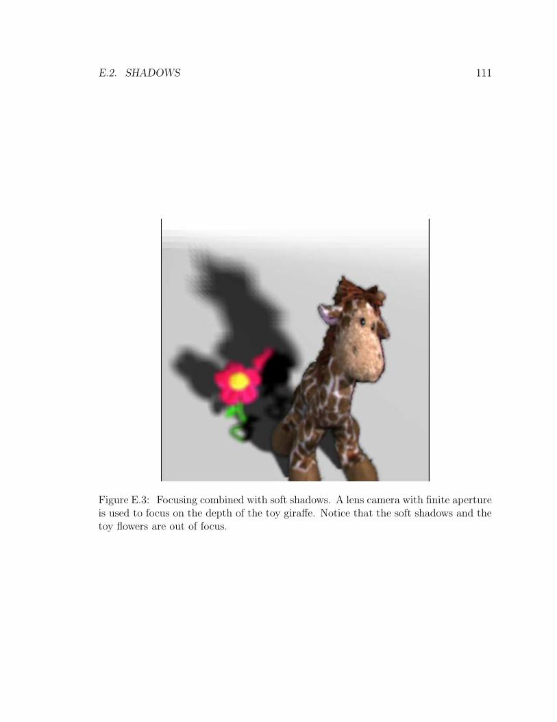
E.2. SHADOWS 111
Figure E.3: Focusing combined with soft shadows. A lens camera with finite apertureis used to focus on the depth of the toy giraffe. Notice that the soft shadows and thetoy flowers are out of focus.

112 APPENDIX E. OTHER LIGHT FIELD MANIPULATIONS

Bibliography
[AB91] Edward H. Adelson and James R. Bergen. The plenoptic function and
the elements of early vision. In Computation Models of Visual Processing,
pages 3–20, 1991. 5, 6
[AF04] Nicholas Apostoloff and Andrew Fitzgibbon. Bayesian video matting
using learnt image priors. In Proceedings of Computer Vision and Pattern
Recognition (CVPR), pages 407–414, 2004. 106
[AMH02] Tomas Akenine-Moller and Eric Haines. Real-time Rendering. A K Pe-
ters, 2002. 63
[Bar84] Alan Barr. Global and local deformations of solid primitives. In Proceed-
ings of SIGGRAPH, pages 21–30, 1984. 35
[Bar04] Brian A. Barsky. Vision-realistic rendering: simulation of the scanned
foveal image from wavefront data of human subjects. In Proceedings
of Symposium on Applied Perception in Graphics and Visualization
(APGV), pages 73–81, New York, NY, USA, 2004. ACM Press. 69
[BBM+01] Chris Buehler, Michael Bosse, Leonard McMillan, Steven J. Gortler, and
Michael F. Cohen. Unstructured lumigraph rendering. In Proceedings of
SIGGRAPH, pages 425–432, 2001. 10, 47
[BSW+05] OpenGL Architecture Review Board, Dave Shreiner, Mason Woo, Jackie
Neider, and Tom Davis. OpenGL(R) Programming Guide : The Official
Guide to Learning OpenGL(R), Version 2 (5th Edition). Addison-Wesley,
2005. 3, 47, 85
113

114 BIBLIOGRAPHY
[CAC+02] Yung-Yu Chuang, Aseem Agarwala, Brian Curless, David H. Salesin,
and Richard Szeliski. Video matting of complex scenes. In Proceedings
of Transactions on Graphics (SIGGRAPH), pages 243–248, 2002. 106
[CCSS01] Yung-Yu Chuang, Brian Curless, David H. Salesin, and Richard Szeliski.
A bayesian approach to digital matting. In Proceedings of Computer
Vision and Pattern Recognition (CVPR), volume 2, pages 264–271. IEEE
Computer Society, December 2001. 103
[CL05] Billy Chen and Hendrik P. A. Lensch. Light source interpolation for
sparsely sampled reflectance fields. In Proceedings of Workshop on Vi-
sion, Modeling and Visualization (VMV), pages 461–468, 2005. 1
[CLF98] Emilio Camahort, Apostolos Lerios, and Don Fussell. Uniformly sampled
light fields. In Proceedings of Eurographics Rendering Workshop, pages
117–130, 1998. 9, 64
[COSL05] Billy Chen, Eyal Ofek, Heung-Yeung Shum, and Marc Levoy. Interactive
deformation of light fields. In Proceedings of Symposium on Interactive
3D Graphics and Games (I3D), pages 139–146, 2005. 1, 47, 91
[CTCS00] Jin-Xiang Chai, Xin Tong, Shing Chow Chan, and Heung-Yeung Shum.
Plenoptic sampling. In Proceedings of SIGGRAPH, pages 307–318, 2000.
7
[CW93] Michael Cohen and John Wallace. Radiosity and Realistic Image Synthe-
sis. Academic Press, 1993. 20
[DHT+00] Paul Debevec, Tim Hawkins, Chris Tchou, Haarm-Pieter Duiker, West-
ley Sarokin, and Mark Sagar. Acquiring the reflectance field of a human
face. In Proceedings of SIGGRAPH, pages 145–156, 2000. 17, 47
[DTM96] Paul E. Debevec, Camillo J. Taylor, and Jitendra Malik. Modeling and
rendering architecture from photographs: A hybrid geometry- and image-
based approach. Proceeedings of Computer Graphics, 30(Annual Confer-
ence Series):11–20, 1996. 7
BIBLIOGRAPHY 115
[EL99] Alexei A. Efros and Thomas K. Leung. Texture synthesis by non-
parametric sampling. In Proceedings of International Conference on
Computer Vision (ICCV), pages 1033–1038, 1999. 41
[FvDFH97] James D. Foley, Andries van Dam, Steven K. Feiner, and John F. Hughes.
Computer Graphics: Principles and Practice. Addison-Wesley, 1997. 6
[GGH03] Michael Goesele, Xavier Granier, Wolfgang Heidrich, and Hans-Peter Sei-
del 1. Accurate light source acquisition and rendering. In Proceedings of
Transactions on Graphics (SIGGRAPH), pages 621–630, 2003. 1
[GGSC96] Steven J. Gortler, Radek Grzeszczuk, Richard Szeliski, and Michael F.
Cohen. The lumigraph. In Proceedings of SIGGRAPH, pages 43–54,
1996. 5, 10, 47
[GLL+04] Michael Goesele, Hendrik P. A. Lensch, Jochen Lang, Christian Fuchs,
and Hans-Peter Seidel. Disco – acquisition of translucent objects. In
Proceedings of Transactions on Graphics (SIGGRAPH), pages 835–844,
2004. 17
[GZN+06] Todor Georgiev, Colin Zheng, Shree K. Nayar, David Salesin, Brian Cur-
less, and Chintan Intwala. Spatio-angular resolution trade-offs in integral
photography. In Proceedings of Eurographics Symposium on Rendering,
pages 263–272, 2006. 11
[HLCS99] Wolfgang Heidrich, Hendrik Lensch, Michael F. Cohen, and Hans-Peter
Seidel. Light field techniques for reflections and refractions. In Proceed-
ings of Eurographics Rendering Workshop, pages 187–196, 1999. 91
[Hor06] Daniel Horn. Vega strike. http://vegastrike.sourceforge.net, 2006. 63
[HZ00] Richard Hartley and Andrew Zisserman. Multiple View Geometry in
computer vision. Press Syndicate of the University of Cambridge, 2000.
28, 105
116 BIBLIOGRAPHY
[HZ03] Richard Hartley and Andrew Zisserman. Multiple View Geometry in
Computer Vision (Second Edition). Press Syndicate of the University of
Cambridge, 2003. 33
[IMG00] Aaron Isaksen, Leonard McMillan, and Steven J. Gortler. Dynamically
reparameterized light fields. In Proceedings of SIGGRAPH, pages 297–
306, 2000. 47, 49
[INH99] Konstantine Iourcha, Krishna Nayak, and Zhou Hong. System and
method for fixed-rate block-based image compression with inferred pixel
values. US Patent 5,956,431, 1999. 53
[Kaj86] James T. Kajiya. The rendering equation. In Proceedings of SIGGRAPH,
pages 143–150. ACM Press / ACM SIGGRAPH, 1986. 6
[KS96] Sing Bing Kang and Rick Szeliski. 3-d scene data recovery using omni-
directional multibaseline stereo. In Proceedings of Computer Vision and
Pattern Recognition (CVPR), pages 167–183, 1996. 15
[LCV+04] Marc Levoy, Billy Chen, Vaibhav Vaish, Mark Horowitz, Ian McDowall,
and Mark Bolas. Synthetic aperture confocal imaging. In Proceedings of
Transactions on Graphics (SIGGRAPH), pages 825–834, 2004. 49
[Lev04a] Marc Levoy. The stanford large statue scanner.
http://graphics.stanford.edu/projects/mich/mgantry-in-lab/mgantry-
in-lab.html, 2004. 10
[Lev04b] Marc Levoy. Stanford spherical gantry.
http://graphics.stanford.edu/projects/gantry, 2004. 10, 74
[LH96] Marc Levoy and Pat Hanrahan. Light field rendering. In Proceedings of
SIGGRAPH, pages 31–42, 1996. 1, 2, 5, 7, 9, 10, 17, 47, 49, 53, 82, 89
[LPC+00] Marc Levoy, Kari Pulli, Brian Curless, Szymon Rusinkiewicz, David
Koller, Lucas Pereira, Matt Ginzton, Sean Anderson, James Davis,

BIBLIOGRAPHY 117
Jeremy Ginsberg, Jonathan Shade, and Duane Fulk. The digital
michelangelo project: 3D scanning of large statues. In Kurt Akeley,
editor, Proceedings of SIGGRAPH, pages 131–144. ACM Press / ACM
SIGGRAPH / Addison Wesley Longman, 2000. 10
[Mag05] Marcus A. Magnor. Video-based Rendering. A K Peters, 2005. 7
[MB95a] Leonard McMillan and Gary Bishop. Plenoptic modeling: An image-
based rendering system. Proceedings of Computer Graphics, 29(Annual
Conference Series):39–46, 1995. 6
[MB95b] Eric N. Mortensen and William A. Barrett. Intelligent scissors for im-
age composition. In Proceedings of Computer graphics and Interactive
Techniques, pages 191–198, 1995. 103
[MBGN98] Tom McReynolds, David Blythe, Brad Grantham, and Scott Nelson.
Programming with opengl: Advanced techniques. In Course 17 notes at
SIGGRAPH 98, 1998. 63
[MG00] Marcus Magnor and Bernd Girod. Data compression for light field ren-
dering. In Proceedings of Transactions on Circuits and Systems for Video
Technology, number 3, pages 338–343, 2000. 53
[MPDW03] Vincent Masselus, Pieter Peers, Philip Dutre, and Yves D. Willems. Re-
lighting with 4d incident light fields. In Proceedings of Transactions on
Graphics (SIGGRAPH), pages 613–620, 2003. 1
[MPN+02] Wojciech Matusik, Hanspeter Pfister, Addy Ngan, Paul Beardsley, Remo
Ziegler, and Leonard McMillan. Image-based 3d photography using opac-
ity hulls. In Proceedings of Transactions on Graphics (SIGGRAPH),
pages 427–437, 2002. 1
[MRG03] Marcus Magnor, Prashant Ramanathan, and Bernd Girod. Multi-view
coding for image-based rendering using 3-d scene geometry. In IEEE

118 BIBLIOGRAPHY
Transactions on Circuits and Systems for Video Technology, pages 1092–
1106, 2003. 53
[MSF02] D. Meneveaux, G. Subrenat, and A. Fournier. Reshading lightfields.
Technical report, IRCOM/SIC, March 2002. No 2002-01. 15
[NLB+05] Ren Ng, Marc Levoy, Mathieu Bredif, Gene Duval, Mark Horowitz, and
Pat Hanrahan. Light field photography with a hand-held plenoptic cam-
era. Technical report, Stanford University, 2005. 11, 56
[Oko76] Takanori Okoshi. Three-Dimensional Imaging Techniques. Academic
Press, 1976. 11
[PD84] Thomas Porter and Tom Duff. Compositing digital images. In Proceed-
ings of Computer Graphics, number 3, pages 253–259, 1984. 90
[Pe01] Ingmar Peter and Wolfgang Straßer. The wavelet stream: Interactive
multi resolution light field rendering. In Proceedings of Eurographics
Rendering Workshop, pages 262–273, 2001. 53
[Per85] Ken Perlin. An image synthesizer. In Proceedings of SIGGRAPH, pages
287–296. ACM Press / ACM SIGGRAPH, 1985. 49, 86
[RNK97] Peter Rander, PJ Narayanan, and Takeo Kanade. Virtualized reality:
Constructing time-varying virtual worlds from real world events. In IEEE
Visualization 1997, pages 277–284, 1997. 11
[Ros04] Randi J. Rost. OpenGL Shading Language. Addison-Wesley, 2004. 53,
55, 86, 87
[SB96] Alvy Ray Smith and James F. Blinn. Blue screen matting. In Proceedings
of Computer Graphics and Interactive Techniques, pages 259–268, 1996.
56, 109
[SCG+05] Pradeep Sen, Billy Chen, Gaurav Garg, Stephen R. Marschner, Mark
Horowitz, Marc Levoy, and Hendrik P. A. Lensch. Dual photography. In

BIBLIOGRAPHY 119
Proceedings of Transactions on Graphics (SIGGRAPH), pages 745–755,
2005. 1
[SH99] Heung-Yeung Shum and Li-Wei He. Rendering with concentric mosaics.
In Proceedings of SIGGRAPH, pages 299–306, 1999. 89
[SK98] Steve Seitz and Kiriakos N. Kutulakos. Plenoptic image editing. In
Proceedings of International Conference on Computer Vision (ICCV),
pages 17–24, 1998. 15
[SP86] Thomas W. Sederberg and Scott R. Parry. Free-form deformation of solid
geometry models. In Proceedings of SIGGRAPH, pages 151–160, 1986.
2, 23, 24
[SS04] Heung-Yeung Shum and Jian Sun. Pop-up light field: An interactive
image-based modeling and rendering system. In Proceedings of Transac-
tions on Graphics, pages 143–162, 2004. 47, 105
[Ups92] Steve Upstill. The RenderMan Companion: A Programmer’s Guide to
Realistic Computer Graphics. Addison-Wesley, 1992. 3, 47
[VWJL04] Vaibhav Vaish, Bennett Wilburn, Neel Joshi, and Marc Levoy. Using
plane + parallax for calibrating dense camera arrays. In Proceedings of
Computer Vision and Pattern Recognition (CVPR), pages 2–9, 2004. 2,
8, 47, 49, 53
[WAA+00] Daniel N. Wood, Daniel I. Azuma, Ken Aldinger, Brian Curless, Tom
Duchamp, David H. Salesin, and Werner Stuetzle. Surface light fields for
3d photography. In Proceedings of SIGGRAPH, pages 287–296, 2000. 7
[WFZ02] Yoni Wexler, Andrew Fitzgibbon, and Andrew Zisserman. Bayesian es-
timation of layers from multiple images. In Proc. ECCV, pages 487–501,
2002. 106
[WJV+05] Bennett Wilburn, Neel Joshi, Vaibhav Vaish, Eino-Ville Talvala, Emilio
Antunez, Adam Barth, Andrew Adams, Mark Horowitz, and Marc Levoy.

120 BIBLIOGRAPHY
High performance imaging using large camera arrays. In Proceedings of
Transactions on Graphics (SIGGRAPH), pages 765–776, 2005. 11, 49
[WL01] Li-Yi Wei and Marc Levoy. Texture synthesis over arbitrary manifold
surfaces. In Proceedings of SIGGRAPH, pages 355–360, 2001. 41
[WPG04] Tim Weyrich, Hanspeter Pfister, and Markus Gross. Rendering de-
formable surface reflectance fields. In Proceedings of Transactions on
Computer Graphics and Visualization, pages 48–58, 2004. 15
[WSLH02] Bennett Wilburn, Michael Smulski, Hsiao-Heng Kelin Lee, and Mark
Horowitz. The light field video camera. In Proceedings of Media Proces-
sors 2002, SPIE Electronic Imaging, 2002. 11
[yaf05] yafray. yafray. http://www.yafray.org/, 2005. 94
[YEBM02] Jason C. Yang, Matthew Everett, Chris Buehler, and Leonard McMillan.
A real-time distributed light field camera. In Proceedings of Eurographics
Rendering Workshop, pages 77–86, 2002. 11
[YM04] Jingyi Yu and Leonard McMillan. General linear cameras. In Proceed-
ings of European Conference on Computer Vision (ECCV), pages 14–27,
2004. 60
[YYM05] Jingyi Yu, Jason Yang, and Leonard McMillan. Real-time reflection
mapping with parallax. In Proceedings of Symposium on Interactive 3D
Graphics and Games (I3D), pages 133–138, 2005. 91
[ZC04] Cha Zhang and Tsuhan Chen. A self-reconfigurable camera array. In
Proceedings of Eurographics Symposium on Rendering, pages 243–254,
2004. 11
[ZKU+04] C. Lawrence Zitnick, Sing Bing Kang, Matthew Uyttendaele, Simon
Winder, and Richard Szeliski. High-quality video view interpolation us-
ing a layered representation. In Proceedings of Transactions on Graphics
(SIGGRAPH), pages 600–608, 2004. 103

BIBLIOGRAPHY 121
[ZWGS02] Zhunping Zhang, Lifeng Wang, Baining Guo, and Heung-Yeung Shum.
Feature-based light field morphing. In Proceedings of Transactions on
Graphics (SIGGRAPH), pages 457–464, 2002. 2, 15, 41, 47