Embed Size (px)
Citation preview

3109 Cornelius Drive
Bloomington, IL 61704 309.807.2300
pinnacleactuaries.com
Commitment Beyond Numbers
Roosevelt C. Mosley, Jr., FCAS, MAAA [email protected]
Direct: 309.807.2330
November 10, 2017
Dana Wade
General Deputy Assistant Secretary
Office of Housing
U.S. Department of Housing and Urban Development
451 Seventh Street, S.W., Room 9100
Washington, D.C. 20410
Dear Ms. Wade:
Pinnacle Actuarial Resources, Inc. (Pinnacle) has completed Fiscal Year 2017 Independent Actuarial
Review of the Mutual Mortgage Insurance Fund. The attached report details our estimate of the Cash
Flow Net Present Value for Fiscal Year 2017.
Roosevelt C. Mosley, Jr., FCAS, MAAA and Thomas R. Kolde, FCAS, MAAA are responsible for the
content and conclusions set forth in the report. We are Fellows of the Casualty Actuarial Society and
Members of the American Academy of Actuaries, and are qualified to render the actuarial opinion
contained herein.
It has been a pleasure working with you and your team to complete this study. We are available for any
questions or comments you have regarding the report and its conclusions.
Respectfully Submitted,
Roosevelt C. Mosley, Jr. FCAS, MAAA Thomas R. Kolde, FCAS, MAAA
Principal and Consulting Actuary Consulting Actuary
3109 Cornelius Drive Bloomington, IL 61704
309.807.2300 pinnacleactuaries.com
Commitment Beyond Numbers
FiscalYear2017IndependentActuarialReviewoftheMutualMortgage
InsuranceFund:CashFlowNetPresentValuefromHomeEquityConversion
MortgageInsurance‐In‐Force
November 10, 2017

Fiscal Year 2017 Independent Actuarial Review of the Mutual Mortgage Insurance Fund: Cash Flow Net Present
Value from Home Equity Conversion Mortgage Insurance‐In‐Force
Commitment Beyond Numbers
Table of Contents
Summary of Findings ................................................................................................................................................. 1
Executive Summary ................................................................................................................................................... 4
Impact of Economic and Mortgage Factors .......................................................................................................... 4
Distribution and Use .................................................................................................................................................. 6
Reliances and Limitations .......................................................................................................................................... 6
Section I. Introduction ............................................................................................................................................... 8
Scope ..................................................................................................................................................................... 8
HECM Background ................................................................................................................................................. 9
Maximum Claim Amount ................................................................................................................................... 9
Principal Limits and Principal Limit Factors ..................................................................................................... 10
Payment Plans ................................................................................................................................................. 10
Unpaid Principal Balance and Mortgage Costs................................................................................................ 10
Mortgage Terminations ................................................................................................................................... 10
Assignments and Recoveries ........................................................................................................................... 11
Report Structure .................................................................................................................................................. 11
Section 2. Summary of Findings .............................................................................................................................. 12
Fiscal Year 2017 Net Present Value Estimate ...................................................................................................... 12
Section 3. HECM Cash Flow NPV Based on Alternative Scenarios .......................................................................... 14
Moody’s Baseline Assumptions ........................................................................................................................... 14
Stronger Near‐Term Growth Scenario ................................................................................................................ 14
Slower Near‐Term Growth Scenario ................................................................................................................... 15
Moderate Recession Scenario ............................................................................................................................. 15
Protracted Slump Scenario .................................................................................................................................. 15
Below‐Trend Long‐Term Growth Scenario .......................................................................................................... 15
Stagflation Scenario ............................................................................................................................................. 15
Next‐Cycle Recession Scenario ............................................................................................................................ 16

Fiscal Year 2017 Independent Actuarial Review of the Mutual Mortgage Insurance Fund: Cash Flow
Net Present Value from Home Equity Conversion Mortgage Insurance‐In‐Force November 10, 2017 Page ii
Pinnacle Actuarial Resources, Inc.
Low Oil Price Scenario ......................................................................................................................................... 16
Summary of Alternative Scenarios ...................................................................................................................... 16
Stochastic Simulation .......................................................................................................................................... 16
Sensitivity Tests of Economic Variables ............................................................................................................... 17
Section 4. Summary of Methodology ...................................................................................................................... 22
Data Sources (Appendix A) .................................................................................................................................. 22
Data Processing – Mortgage‐Level Modeling ...................................................................................................... 23
Data Reconciliation .............................................................................................................................................. 24
HECM Base Termination Model (Appendix B) ..................................................................................................... 25
HECM Cash Flow Draw Projection Models (Appendix C) .................................................................................... 26
HECM Cash Flow Analysis (Appendix E) .............................................................................................................. 26
Cash Flow Components ................................................................................................................................... 26
Net Future Cash Flows ..................................................................................................................................... 27
Discount Factors .............................................................................................................................................. 27
Appendices .............................................................................................................................................................. 28
Appendix A: Data Sources, Processing and Reconciliation ..................................................................................... 29
Data Processing – Mortgage Level Modeling ...................................................................................................... 30
Data Reconciliation .............................................................................................................................................. 30
Appendix B: HECM Base Termination Model .......................................................................................................... 33
Model Specification ............................................................................................................................................. 33
Multinomial Logistic Regression Theory ......................................................................................................... 34
Explanatory Variables .......................................................................................................................................... 35
Model Validation ................................................................................................................................................. 36
Appendix C: HECM Cash Draw Projection Models .................................................................................................. 43
Likelihood of a Cash Draw ................................................................................................................................... 43
Estimated Cash Draw Amount ............................................................................................................................. 43
Appendix D: Economic Scenarios ............................................................................................................................ 44
Alternative Scenarios ........................................................................................................................................... 44
Graphical Depiction of the Scenarios .................................................................................................................. 45

Fiscal Year 2017 Independent Actuarial Review of the Mutual Mortgage Insurance Fund: Cash Flow
Net Present Value from Home Equity Conversion Mortgage Insurance‐In‐Force November 10, 2017 Page iii
Pinnacle Actuarial Resources, Inc.
Stochastic Simulations ......................................................................................................................................... 47
Historical Data ................................................................................................................................................. 48
Modeling Techniques ...................................................................................................................................... 51
1‐Year CMT Rate .............................................................................................................................................. 51
Additional Interest Rate Models ..................................................................................................................... 53
HPA .................................................................................................................................................................. 54
Unemployment Rate ....................................................................................................................................... 56
Gross Domestic Product .................................................................................................................................. 57
Final Simulation Selection ............................................................................................................................... 57
Appendix E: HECM Cash Flow Analysis .................................................................................................................... 58
General Approach to Mortgage Termination Projections ................................................................................... 58
Cash Flow Components ....................................................................................................................................... 58
Mortgage Balance ............................................................................................................................................ 59
Tax & Insurance Defaults ................................................................................................................................. 59
MIP .................................................................................................................................................................. 60
Claims .............................................................................................................................................................. 60
Note Holding Expenses After Assignment ....................................................................................................... 62
Recoveries from Assigned Mortgages ............................................................................................................. 62
Net Future Cash Flows ......................................................................................................................................... 63
Discount Factors .................................................................................................................................................. 63
Fiscal Year 2017 Independent Actuarial Review of the Mutual Mortgage Insurance Fund: Cash Flow Net Present
Value from Home Equity Conversion Mortgage Insurance‐In‐Force
Commitment Beyond Numbers
Summary of Findings This report presents the results of Pinnacle Actuarial Resources, Inc.’s (Pinnacle) independent actuarial review of
the Cash Flow Net Present Value (NPV) associated with Home Equity Conversion Mortgages (HECM) insured by
the Mutual Mortgage Insurance Fund (MMIF) for fiscal year 2017. The Cash Flow NPV associated with forward
mortgages are analyzed separately and are excluded from this report. In the remainder of this report, the term
MMIF refers to HECMs and excludes forward mortgages.
Below, we summarize the findings associated with each of the required deliverables.
Deliverable 1: The Actuary’s conclusion regarding the reasonableness of Federal Housing Administration’s
(FHA) estimate of Cash Flow Net Present Value from Home Equity Conversion Mortgage Insurance‐In‐Force as
presented in FHA’s Annual Report to Congress and the Actuary’s best estimate of the range of reasonable
estimates, including the 90th, 95th and 99th percentiles.
As of the end of Fiscal Year 2017, Pinnacle’s Actuarial Central Estimate (ACE) of the MMIF HECM Cash Flow NPV
is negative $14.2 billion. Pinnacle’s ACE is based on the Economic Assumptions for the 2018 Budget Fall Baseline
from the Office of Management and Budget (OMB Economic Assumptions).
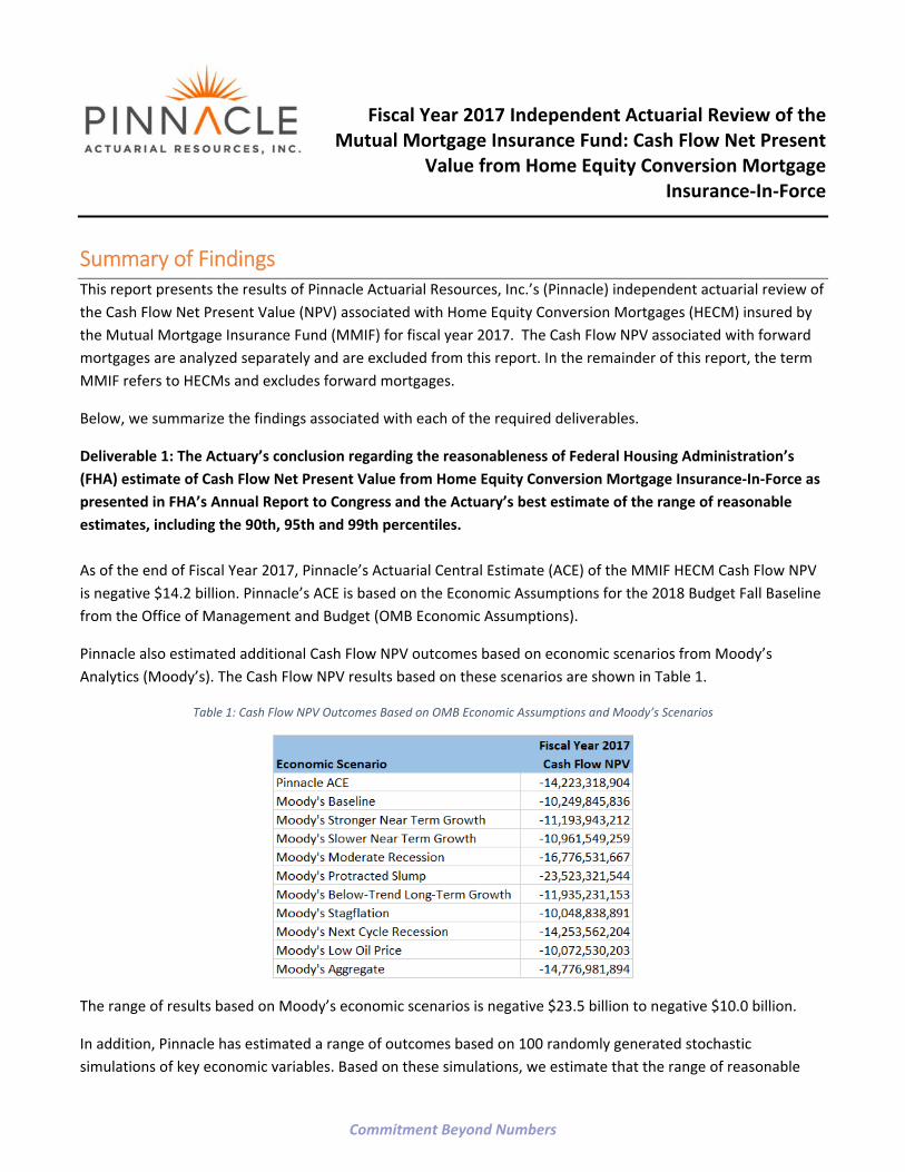
Pinnacle also estimated additional Cash Flow NPV outcomes based on economic scenarios from Moody’s
Analytics (Moody’s). The Cash Flow NPV results based on these scenarios are shown in Table 1.
Table 1: Cash Flow NPV Outcomes Based on OMB Economic Assumptions and Moody’s Scenarios
The range of results based on Moody’s economic scenarios is negative $23.5 billion to negative $10.0 billion.
In addition, Pinnacle has estimated a range of outcomes based on 100 randomly generated stochastic
simulations of key economic variables. Based on these simulations, we estimate that the range of reasonable

Fiscal Year 2017 Independent Actuarial Review of the Mutual Mortgage Insurance Fund: Cash Flow
Net Present Value from Home Equity Conversion Mortgage Insurance‐In‐Force November 10, 2017 Page 2
Pinnacle Actuarial Resources, Inc.
Cash Flow NPV estimates is negative $20.4 billion to negative $7.6 billion. This range is based on an 80%
likelihood that the ultimate Cash Flow NPV will fall within the lower and upper bound of the range. The 90th, 95th
and 99th percentiles of the stochastic simulations are shown below:
90th percentile: ‐ $7.6 billion
95th percentile: ‐ $5.7 billion
99th percentile: ‐ $3.2 billion
The Cash Flow NPV estimate provided by FHA to be used in the FHA’s Annual Report to Congress is negative
$15.5 billion. Based on Pinnacle’s ACE and range of reasonable estimates, we conclude that the FHA estimate of
Cash Flow NPV is reasonable.
Deliverable 2: The Actuary’s best estimate and range of reasonable estimates of Cash Flow Net Present Value
by cohort from Home Equity Conversion Mortgage Insurance‐In‐Force as presented in FHA’s Annual Report to
Congress.
Pinnacle’s ACE and range of reasonable estimates of the Cash Flow NPV by cohort are shown below. The range
of estimates are based on the stochastic simulation results.
Table 2: Range of Reasonable Estimates ‐ HECM Cash Flow NPV
Deliverable 3: Reconciliation of the data used to prepare Pinnacle’s estimates with data used by FHA to
prepare its estimated Cash Flow NPV.
Section 4 shows the reconciliation of the data used by Pinnacle with the data used by FHA. Please see the
section titled Data Reconciliation.
Deliverable 4: Assumptions and judgments on which estimates are based, support for the assumptions and
sensitivity of the estimates to alternative assumptions and judgments.

Fiscal Year 2017 Independent Actuarial Review of the Mutual Mortgage Insurance Fund: Cash Flow
Net Present Value from Home Equity Conversion Mortgage Insurance‐In‐Force November 10, 2017 Page 3
Pinnacle Actuarial Resources, Inc.
The assumptions and judgments on which the estimates are based are summarized in Section 4. The section
titled HECM Base Termination Model summarizes the specifications and assumptions related to the base
termination models. The HECM Cash Flow Draw Projection Models section summarizes the cash draw models
for HECM mortgages with lines of credit. Section 3 discusses the economic assumptions incorporated into the
estimates. Lastly, the HECM Cash Flow Analysis section of Section 4 details the assumptions associated with the
cash flow projections. Section 3 also shows the sensitivity of the estimates to alternative economic scenarios.
Deliverable 5: Narrative component that provides detail to explain to FHA and the Department of Housing and
Urban Development (HUD) management and auditors, OMB and Congressional offices the findings and their
significance, and technical component that traces the analysis from the data to the conclusions.
Sections 1 and 2 provide an explanation of the findings and the significance of the findings. Also, Section 4 traces
the analysis from data to conclusions.
Deliverable 6: Commentary on the likelihood of risks and uncertainties that could result in material adverse
changes in the condition of the MMIF HECM portfolio as measured by the Cash Flow NPV.
Section 3 provides a discussion of the economic conditions that could result in material adverse condition of the
Cash Flow NPV.
Fiscal Year 2017 Independent Actuarial Review of the Mutual Mortgage Insurance Fund: Cash Flow
Net Present Value from Home Equity Conversion Mortgage Insurance‐In‐Force November 10, 2017 Page 4
Pinnacle Actuarial Resources, Inc.
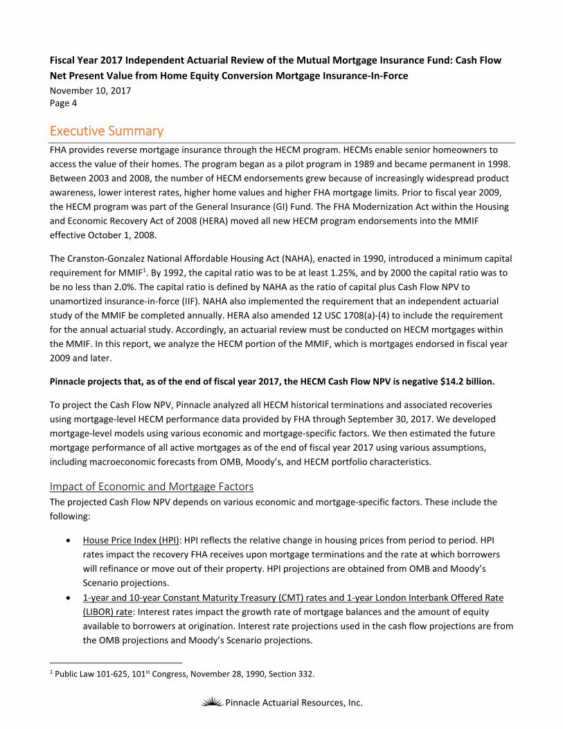
Executive Summary FHA provides reverse mortgage insurance through the HECM program. HECMs enable senior homeowners to
access the value of their homes. The program began as a pilot program in 1989 and became permanent in 1998.
Between 2003 and 2008, the number of HECM endorsements grew because of increasingly widespread product
awareness, lower interest rates, higher home values and higher FHA mortgage limits. Prior to fiscal year 2009,
the HECM program was part of the General Insurance (GI) Fund. The FHA Modernization Act within the Housing
and Economic Recovery Act of 2008 (HERA) moved all new HECM program endorsements into the MMIF
effective October 1, 2008.
The Cranston‐Gonzalez National Affordable Housing Act (NAHA), enacted in 1990, introduced a minimum capital
requirement for MMIF1. By 1992, the capital ratio was to be at least 1.25%, and by 2000 the capital ratio was to
be no less than 2.0%. The capital ratio is defined by NAHA as the ratio of capital plus Cash Flow NPV to
unamortized insurance‐in‐force (IIF). NAHA also implemented the requirement that an independent actuarial
study of the MMIF be completed annually. HERA also amended 12 USC 1708(a)‐(4) to include the requirement
for the annual actuarial study. Accordingly, an actuarial review must be conducted on HECM mortgages within
the MMIF. In this report, we analyze the HECM portion of the MMIF, which is mortgages endorsed in fiscal year
2009 and later.
Pinnacle projects that, as of the end of fiscal year 2017, the HECM Cash Flow NPV is negative $14.2 billion.
To project the Cash Flow NPV, Pinnacle analyzed all HECM historical terminations and associated recoveries
using mortgage‐level HECM performance data provided by FHA through September 30, 2017. We developed
mortgage‐level models using various economic and mortgage‐specific factors. We then estimated the future
mortgage performance of all active mortgages as of the end of fiscal year 2017 using various assumptions,
including macroeconomic forecasts from OMB, Moody’s, and HECM portfolio characteristics.
Impact of Economic and Mortgage Factors
The projected Cash Flow NPV depends on various economic and mortgage‐specific factors. These include the
following:
House Price Index (HPI): HPI reflects the relative change in housing prices from period to period. HPI
rates impact the recovery FHA receives upon mortgage terminations and the rate at which borrowers
will refinance or move out of their property. HPI projections are obtained from OMB and Moody’s
Scenario projections.
1‐year and 10‐year Constant Maturity Treasury (CMT) rates and 1‐year London Interbank Offered Rate
(LIBOR) rate: Interest rates impact the growth rate of mortgage balances and the amount of equity
available to borrowers at origination. Interest rate projections used in the cash flow projections are from
the OMB projections and Moody’s Scenario projections.
1 Public Law 101‐625, 101st Congress, November 28, 1990, Section 332.
Fiscal Year 2017 Independent Actuarial Review of the Mutual Mortgage Insurance Fund: Cash Flow
Net Present Value from Home Equity Conversion Mortgage Insurance‐In‐Force November 10, 2017 Page 5
Pinnacle Actuarial Resources, Inc.
Mortality Rates: Information on the date of death of borrowers and co‐borrowers have either been
directly obtained or derived from the U.S. Decennial Life Table for the 1990‐1991, 1999‐2001, and 2001‐
2012 populations, published by the Center for Disease Control and Prevention (CDC) or from the Social
Security Administration.
Cash Drawdown Rates: These rates represent the speed at which borrowers access the equity in their
homes over time, which impacts the growth of the mortgage balance. Predictive models have been
developed to estimate borrower cash draw rates based on past HECM program experience, borrower
characteristics and the economic environment.
The realized Cash Flow NPV will vary from the estimates in this analysis if the actual drivers of mortgage
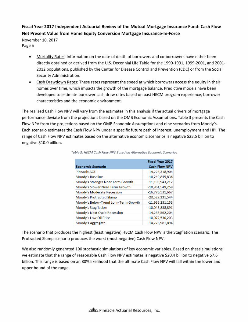
performance deviate from the projections based on the OMB Economic Assumptions. Table 3 presents the Cash
Flow NPV from the projections based on the OMB Economic Assumptions and nine scenarios from Moody’s.
Each scenario estimates the Cash Flow NPV under a specific future path of interest, unemployment and HPI. The
range of Cash Flow NPV estimates based on the alternative economic scenarios is negative $23.5 billion to
negative $10.0 billion.
Table 3: HECM Cash Flow NPV Based on Alternative Economic Scenarios
The scenario that produces the highest (least negative) HECM Cash Flow NPV is the Stagflation scenario. The
Protracted Slump scenario produces the worst (most negative) Cash Flow NPV.
We also randomly generated 100 stochastic simulations of key economic variables. Based on these simulations,
we estimate that the range of reasonable Cash Flow NPV estimates is negative $20.4 billion to negative $7.6
billion. This range is based on an 80% likelihood that the ultimate Cash Flow NPV will fall within the lower and
upper bound of the range.

Fiscal Year 2017 Independent Actuarial Review of the Mutual Mortgage Insurance Fund: Cash Flow
Net Present Value from Home Equity Conversion Mortgage Insurance‐In‐Force November 10, 2017 Page 6
Pinnacle Actuarial Resources, Inc.
Distribution and Use This report is being provided to FHA for their use and the use of makers of public policy in evaluating the Cash
Flow NPV of the MMIF. Permission is hereby granted for its distribution on the condition that the entire report,
including the exhibits and appendices, is distributed rather than any excerpt. Pinnacle also acknowledges that
excerpts of this report will be used in preparing summary comparisons for FHA’s Annual Report to Congress, and
permission is granted for this purpose as well. We are available to answer any questions that may arise
regarding this report.
Any third parties receiving the report should recognize that the furnishing of this report is not a substitute for
their own due diligence and should place no reliance on this report or the data contained herein that would
result in the creation of any duty or liability by Pinnacle to the third party.
Our conclusions are predicated on a number of assumptions as to future conditions and events. These
assumptions, which are documented in subsequent sections of the report, must be understood in order to place
our conclusions in their appropriate context. In addition, our work is subject to inherent limitations, which are
also discussed in this report.
Reliances and Limitations Listed in Section 4 are the data sources Pinnacle has relied on in our analysis. We have relied on the accuracy of
these data sources in our calculations. If it is subsequently discovered that the underlying data or information is
erroneous, then our calculations would need to be revised accordingly.
We have relied on a significant amount of data and information without auditing or verifying the accuracy of the
data. This includes economic data projected over the next 30 years from Moody’s and the OMB. However, we
did review as many elements of the data and information as practical for reasonableness and consistency with
our knowledge of the mortgage insurance industry. It is possible that the historical data used to develop our
estimates may not be predictive of future default and loss experience. We have not anticipated any
extraordinary changes to the legal, social or economic environment which might affect the number or cost of
mortgage defaults beyond those contemplated in the economic scenarios described in this report. To the extent
that realized experience deviates significantly from these assumptions, the actual results may differ, perhaps
significantly, from estimated results.
The predictive models used in this analysis are based on a theoretical framework and certain assumptions.
These models predict the termination rates, cash flow draws and net loss based on a number of individual
mortgage characteristics and economic variables. The parameters of the predictive models are estimated over a
wide variety of mortgages that originated since 1989 and their performance under the range of economic
conditions and mortgage market environments experienced. The models are combined with assumptions about
future mortgage endorsements and certain key economic assumptions to produce future projections of the Cash
Flow NPV. Although the models are based on mortgages from as far back as 1989, the results presented in the
report are only related to mortgages endorsed in fiscal year 2009 and later, as this is when the HECM mortgages

Fiscal Year 2017 Independent Actuarial Review of the Mutual Mortgage Insurance Fund: Cash Flow
Net Present Value from Home Equity Conversion Mortgage Insurance‐In‐Force November 10, 2017 Page 7
Pinnacle Actuarial Resources, Inc.
were added to the MMIF.
Pinnacle is not qualified to provide formal legal interpretation of federal legislation or FHA policies and
procedures. The elements of this report that require legal interpretation should be recognized as reasonable
interpretations of the available statutes, regulations and administrative rules.
Fiscal Year 2017 Independent Actuarial Review of the Mutual Mortgage Insurance Fund: Cash Flow
Net Present Value from Home Equity Conversion Mortgage Insurance‐In‐Force November 10, 2017 Page 8
Pinnacle Actuarial Resources, Inc.
Section I. Introduction
Scope
FHA has engaged Pinnacle to perform an annual independent actuarial study of the MMIF. This study is required
by 12 USC 1708(a)‐(4) and must be completed in compliance with the Federal Credit Reform Act as implemented
and all applicable Actuarial Standards of Practice (ASOPs).
The FHA Modernization Act within the HERA moved all new endorsements for FHA’s HECM program from the GI
Fund to the MMIF starting in fiscal year 2009. Therefore, an actuarial review must also be conducted on the
HECM portfolio within the MMIF. This report provides the estimated HECM Cash Flow NPV as of September 30,
2017.
The MMIF is a group of accounts of the federal government which records transactions associated with the
FHA’s guaranty programs for single family mortgages. Currently, the FHA insures approximately 7.82 million
forward mortgages under the MMIF and 440,000 reverse mortgages under the HECM program.
Per 12 USC 1711‐(f), the FHA must ensure that the MMIF maintains a capital ratio of not less than 2.0%. The
capital ratio is defined as the ratio of capital to MMIF obligations on outstanding mortgages (IIF). Capital is
defined as cash available to the Fund plus the Cash Flow NPV that is expected to result from the outstanding
HECMs insured by the MMIF.
The deliverables included in this study are:
1. The Actuary’s conclusion regarding the reasonableness of FHA’s estimate of Cash Flow NPV from Home
Equity Conversion Mortgage Insurance‐In‐Force as presented in FHA’s Annual Report to Congress and
the Actuary’s best estimate of the range of reasonable estimates, including the 90th, 95th and 99th
percentiles.
2. The Actuary’s best estimate and range of reasonable estimates of Cash Flow NPV by cohort from Home
Equity Conversion Mortgage Insurance‐In‐Force as presented in FHA’s Annual Report to Congress.
3. Reconciliation of the data used to prepare Pinnacle’s estimates with data used by FHA to prepare its
estimated Cash Flow NPV.
4. Assumptions and judgments on which estimates are based, support for the assumptions and sensitivity
of the estimates to alternative assumptions and judgments.
5. Narrative component that provides detail to explain to FHA and HUD management and auditors, OMB
and Congressional offices the findings and their significance, and a technical component that traces the
analysis from the data to the conclusions.

Fiscal Year 2017 Independent Actuarial Review of the Mutual Mortgage Insurance Fund: Cash Flow
Net Present Value from Home Equity Conversion Mortgage Insurance‐In‐Force November 10, 2017 Page 9
Pinnacle Actuarial Resources, Inc.
6. Commentary on the likelihood of risks and uncertainties that could result in material adverse changes in
the condition of the MMIF as measured by the Cash Flow NPV.
HECM Background
FHA insures reverse mortgages through the HECM program, which enables senior homeowners to borrow
against the value of their homes. Since the inception of the HECM program in 1989, FHA has insured just over
one million reverse mortgages. The following conditions must be met to be eligible for a HECM:
1. at least one of the homeowners must be 62 years of age or older,
2. if there is an existing mortgage, the outstanding balance must be paid off with the HECM proceeds and
3. the borrower(s) must have received FHA‐approved reverse mortgage counseling to learn about the
program.
HECM’s are available from FHA‐approved lending institutions. These approved institutions provide homeowners
with cash payments or lines of credit secured by the collateral property. There is no required repayment as long
as the borrowers continue to live in the home and meet FHA guidelines on requirements for paying property
taxes and homeowner’s insurance premiums and for maintaining the property in a reasonable condition. A
HECM terminates for reasons including death, moving out of the home and refinance. The existence of negative
equity does not require borrowers to pay off the mortgage and it does not prevent the borrowers from receiving
additional cash draws if available based on their HECM contract.
The reverse mortgage insurance provided by FHA through the HECM program protects lenders from losses due
to insufficient recovery on terminated mortgages. When a mortgage terminates and the mortgage balance is
greater than the net sale price of the home, the lender can file a claim for loss up to the maximum claim amount
(MCA). A lender can assign the mortgage note to FHA if the mortgage meets the eligibility requirements when
the mortgage balance reaches 98% of the MCA. On assignment, the lender is reimbursed for the balance of the
mortgage (up to the MCA). When note assignment occurs, FHA switches from being the insurer to the holder of
the note and controls the servicing of the mortgage until termination. At mortgage termination (post‐
assignment), FHA attempts to recover the mortgage balance including any expenses, accrued interest, property
taxes and insurance premiums.
The following are definitions of common HECM terms.
Maximum Claim Amount
The MCA is the minimum of the appraised value or purchase price of the home and the FHA mortgage limit at
the time of origination. It is the maximum HECM insurance claim a lender can receive. The MCA is also used
together with the Principal Limit Factor (PLF) to calculate the maximum amount of initial credit available to the
borrower. The MCA is determined at origination and does not change over the life of the mortgage. However, if
the home value appreciates over time, borrowers may access additional credit by refinancing. In the event of
termination, the entire net sales proceeds can be used to pay off the outstanding mortgage balance, regardless
of whether the size of the MCA was capped by the FHA mortgage limit at origination.

Fiscal Year 2017 Independent Actuarial Review of the Mutual Mortgage Insurance Fund: Cash Flow
Net Present Value from Home Equity Conversion Mortgage Insurance‐In‐Force November 10, 2017 Page 10
Pinnacle Actuarial Resources, Inc.
Principal Limits and Principal Limit Factors
FHA manages its insurance risk by limiting the percentage of the initial available equity that a HECM borrower
can draw by use of a PLF. The PLF is similar conceptually to the loan‐to‐value (LTV) ratio applied to a traditional
mortgage. For a HECM, the MCA is multiplied by the PLF, which is determined according to the HECM program
features and the borrower’s age and gender. The result is the maximum HECM Principal Limit (PL) available to
be drawn by the applicant. The PLF increases with the borrower’s age at HECM origination and decreases as the
expected mortgage interest rate increases. Over the course of the mortgage, the PL grows at a rate equal to the
sum of the mortgage interest, the Mortgage Insurance Premium (MIP) and the servicing fees. Borrowers can
continue to draw cash as long as the mortgage balance is below the current PL (except for the tenure plan,
which acts as an annuity)2.
Payment Plans
HECM borrowers access the equity available to them according to the payment plan they select. Borrowers can
change their payment plan at any time during the course of the mortgage as long as they have not exhausted
their PL. The payment plans are:
Tenure plan: a fixed monthly cash payment as long as the borrowers stay in their home;
Term plan: a fixed monthly cash payment over a specified number of years;
Line of credit: the ability to draw on allowable funds at any time; and
Any combination of the above.
Under the current program, the initial disbursement period limitation is applicable to all payment plans and
subsequent payment plan changes that occur during the initial disbursement period.
Unpaid Principal Balance and Mortgage Costs
The Unpaid Principal Balance (UPB) is the mortgage balance and represents the amount drawn from the HECM.
In general, after the initial cash draw, the mortgage balance continues to grow with additional borrower cash
draws and accruals of interest, premiums and servicing fees until the mortgage terminates.
Mortgage Terminations
When a HECM terminates, the current mortgage balance becomes due. If the net sales proceeds from the home
sale exceed the mortgage balance, the borrower or the estate is entitled to the difference. If the net proceeds
from the home sale are insufficient to pay off the full outstanding mortgage balance and the lender has not
assigned the note, the lender can file a claim for the shortfall, up to the amount of the MCA. HECMs are non‐
recourse, so the property is the only collateral for the mortgage; no other assets or the income of the borrowers
can be accessed to cover any shortfall.
2 Mortgagee Letter 97‐15, April 24, 1997: Home Equity Conversion Mortgage (HECM) Insurance Program – Implementation of Final Rule and Other Information.

Fiscal Year 2017 Independent Actuarial Review of the Mutual Mortgage Insurance Fund: Cash Flow
Net Present Value from Home Equity Conversion Mortgage Insurance‐In‐Force November 10, 2017 Page 11
Pinnacle Actuarial Resources, Inc.
Assignments and Recoveries
The assignment option is a unique feature of the HECM program. When the balance of a HECM reaches 98% of
the MCA and meets other assignment requirements, the lender can choose to terminate the FHA insurance by
redeeming the mortgage note with FHA at face value, a transaction referred to as mortgage assignment. FHA
will pay an assignment claim in the full amount of the mortgage balance (up to the MCA) and will continue to
hold the note until termination. During the note holding period, the mortgage balance will continue to grow by
additional draws and unpaid taxes and insurance. Borrowers can continue to draw cash as long as the mortgage
balance is below the current PL. The only exception is that borrowers on the tenure plan are not constrained by
the PL. At mortgage termination, the borrowers or their estates are required to repay FHA the minimum of the
mortgage balance and the net sales proceeds of the home. These repayments are referred to as post‐
assignment recoveries.
Report Structure
The remainder of this report consists of the following sections:
Section 2. Summary of Findings – presents the estimated Cash Flow NPV for the HECM portfolio as of
the end of fiscal year 2017.
Section 3. HECM NPV Based on Alternative Scenarios – presents the HECM portfolio Cash Flow NPV
using alternative economic scenarios.
Section 4. Summary of Methodology – presents an overview of the data processing and reconciliation,
base termination models, cash draw models for mortgages with a line of credit and cash flow models
used to estimate the Cash Flow NPV.
Fiscal Year 2017 Independent Actuarial Review of the Mutual Mortgage Insurance Fund: Cash Flow
Net Present Value from Home Equity Conversion Mortgage Insurance‐In‐Force November 10, 2017 Page 12
Pinnacle Actuarial Resources, Inc.
Section 2. Summary of Findings This section presents the projected HECM Cash Flow NPV for fiscal year 2017. This review covers mortgages that
were endorsed in fiscal year 2009 and subsequent and are still in force as of the end of fiscal year 2017. Data
through September 30, 2017 was used to estimate the Cash Flow NPV.
Fiscal Year 2017 Net Present Value Estimate
The Cash Flow NPV of in‐force HECM’s consists of discounted cash inflows and outflows. HECM cash inflows
consist of MIP and recoveries. Cash outflows consist of claims and note‐holding expenses. The cash flow model
projects cash inflows and outflows using economic forecasts and mortgage performance projections. The Cash
Flow NPV is estimated to be negative $14.2 billion as of the end of fiscal year 2017. This estimate is the result of
the cash flow projections resulting from the OMB President’s Economic Assumptions for Fiscal Year 2017.
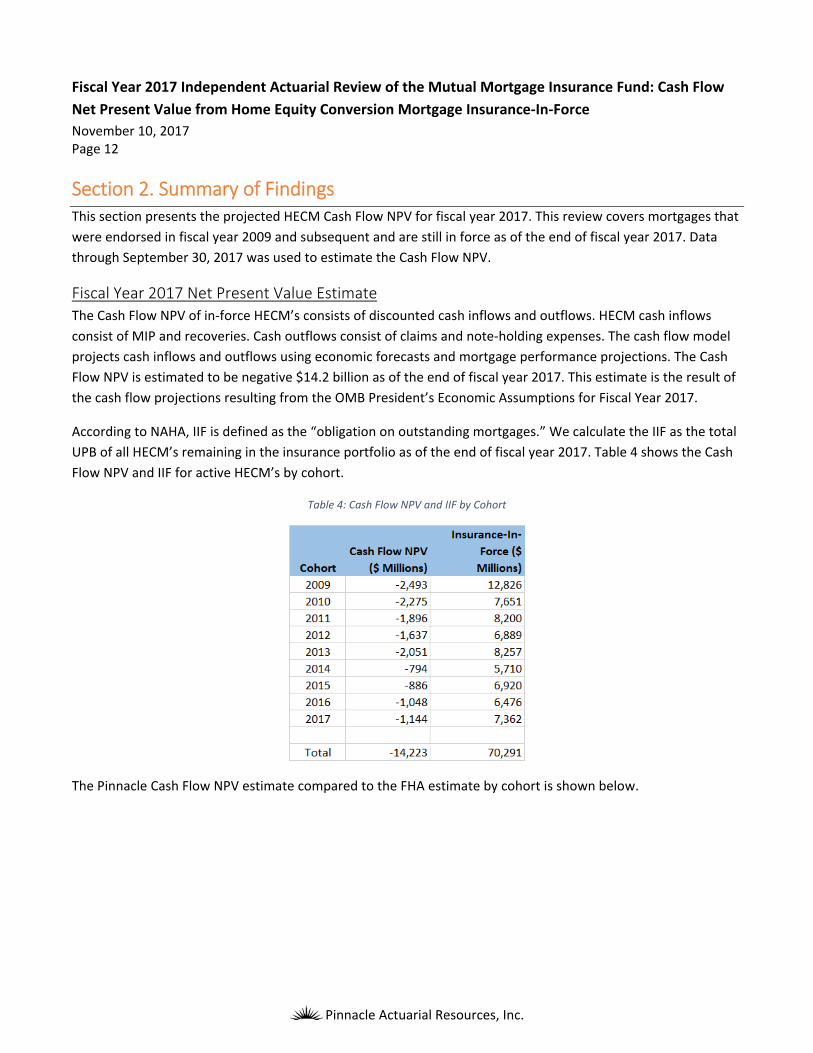
According to NAHA, IIF is defined as the “obligation on outstanding mortgages.” We calculate the IIF as the total
UPB of all HECM’s remaining in the insurance portfolio as of the end of fiscal year 2017. Table 4 shows the Cash
Flow NPV and IIF for active HECM’s by cohort.
Table 4: Cash Flow NPV and IIF by Cohort
The Pinnacle Cash Flow NPV estimate compared to the FHA estimate by cohort is shown below.
Fiscal Year 2017 Independent Actuarial Review of the Mutual Mortgage Insurance Fund: Cash Flow
Net Present Value from Home Equity Conversion Mortgage Insurance‐In‐Force November 10, 2017 Page 13
Pinnacle Actuarial Resources, Inc.
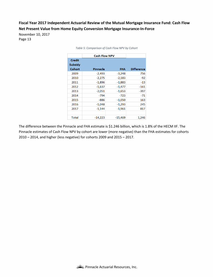
Table 5: Comparison of Cash Flow NPV by Cohort
The difference between the Pinnacle and FHA estimate is $1.246 billion, which is 1.8% of the HECM IIF. The
Pinnacle estimates of Cash Flow NPV by cohort are lower (more negative) than the FHA estimates for cohorts
2010 – 2014, and higher (less negative) for cohorts 2009 and 2015 – 2017.

Fiscal Year 2017 Independent Actuarial Review of the Mutual Mortgage Insurance Fund: Cash Flow
Net Present Value from Home Equity Conversion Mortgage Insurance‐In‐Force November 10, 2017 Page 14
Pinnacle Actuarial Resources, Inc.
Section 3. HECM Cash Flow NPV Based on Alternative Scenarios The Cash Flow NPV will vary from our estimates if the actual drivers of mortgage performance deviate from the
projections based on the OMB Economic Assumptions. In this section, we develop additional estimates of the
Cash Flow NPV based on the following:
1. Moody’s Economic Scenarios
2. Stochastic simulation of key economic variables
3. Sensitivity testing of key economic variables
Each Moody’s scenario produces an estimate of the Cash Flow NPV using the future interest, unemployment and
HPI rates as a deterministic path.
The Moody’s scenarios are:
Moody’s Baseline
Stronger Near‐Term Growth
Slower Near‐Term Growth
Moderate Recession
Protracted Slump
Below‐Trend Long‐Term Growth
Stagflation
Next‐Cycle Recession
Low Oil Price
The resulting Cash Flow NPV associated with each alternative scenario is summarized in Table 6.
Moody’s Baseline Assumptions
In this scenario, the HPI increases over the entire projection period, and the rate of change is consistently
between 2.0% and 3.5%. This is different from the OMB Economic Assumptions in that the Moody’s baseline
grows more slowly for the first four years, and then increases at a faster rate through 2027. The mortgage
interest rate increases more slowly than the OMB Economic Assumptions scenario, and settles at a longer term
average of about 5.5%, which is lower than the OMB Economic Assumptions long term estimate of just over
6.0%. The unemployment rate decreases slightly to 3.7% over the next year, and then increases to a long‐term
average of around 5.0%. The OMB estimate decreases to about 4.4% over the next year, and then increases to a
long‐term average of 4.8%.
Stronger Near‐Term Growth Scenario
In the Moody’s Stronger Near‐Term Growth scenario, the HPI is projected to increase more quickly than under
the OMB scenario. In addition, mortgage interest rates are projected to be lower than the OMB estimates
through 2018, then projected to be higher than OMB through 2020, then decrease to a long‐term average of

Fiscal Year 2017 Independent Actuarial Review of the Mutual Mortgage Insurance Fund: Cash Flow
Net Present Value from Home Equity Conversion Mortgage Insurance‐In‐Force November 10, 2017 Page 15
Pinnacle Actuarial Resources, Inc.
just under 5.5%. The unemployment rate also is lower than projected in the OMB scenario and remains lower
throughout the entire projection period.
Slower Near‐Term Growth Scenario
In the Moody’s Slower Near‐Term Growth scenario, the HPI increases more slowly than in the OMB scenario,
and near the end of the projection period recovers to the level of the OMB assumptions. Mortgage interest rates
are projected to be lower than the OMB assumptions throughout the projection period, settling at a long‐term
average of just over 5.5%. The unemployment rate is projected to be almost 0.70 points higher than the OMB
assumptions scenario by 2021, and then recovers to just 0.25 points higher than the OMB assumptions in the
long‐term.
Moderate Recession Scenario
In the Moderate Recession scenario, the HPI decreases over the next 18 months, and then begins to increase.
Despite the recovery, the projected HPI is lower than the OMB assumptions for the entire projection period.
Mortgage interest rates spike sharply in the fourth quarter of 2017, and then drop significantly through the first
quarter of 2019. Mortgage rates then begin to slowly increase until they reach the long‐term average of just
over 5.5%. The unemployment rate spikes to almost 8% by 2019, and then recovers to a long‐term average of
just over 5%. The projected unemployment rate is higher than the OMB assumptions for the entire projection
period.
Protracted Slump Scenario
In the Moody’s Protracted Slump scenario, the HPI decreases significantly over the next 18 months, and then
begins to increase again. Despite the recovery, the projected HPI is lower than the OMB assumptions for the
entire projection period. Mortgage interest rates spike sharply in the fourth quarter of 2017, and then drop until
the fourth quarter of 2019. They begin to slowly increase until they reach the long term average of just over
5.5%. The unemployment rate spikes to over 10% by 2020, and then recovers to a long‐term average of
approximately 5.4%. The projected unemployment rate is higher than the OMB scenario for the entire
projection period.
Below‐Trend Long‐Term Growth Scenario
In the Moody’s Below‐Trend Long‐Term Growth scenario, the HPI increases more slowly than in the OMB
assumptions and remains lower for the entire projection period. Mortgage interest rates increase gradually and
settle at a long‐term average of about 5.7%. The projected mortgage interest rate is lower than the OMB
projection over the entire period. The unemployment rate increases to 5.6% by 2020, and then decreases to a
long‐term average of approximately 5.0%.
Stagflation Scenario
In the Moody’s Stagflation scenario, the HPI decreases through the third quarter of 2019, and then begins to
increase. Despite the recovery, the projected HPI is lower than the OMB assumptions for the entire projection
period. Mortgage interest rates increase sharply to 6.8% by the second quarter of 2018, and then drop through

Fiscal Year 2017 Independent Actuarial Review of the Mutual Mortgage Insurance Fund: Cash Flow
Net Present Value from Home Equity Conversion Mortgage Insurance‐In‐Force November 10, 2017 Page 16
Pinnacle Actuarial Resources, Inc.
the second quarter of 2019. They then begin to slowly increase to the long‐term average of just over 5.5%.
Unemployment rates increase significantly to just over 8% by 2019, and then decrease to a long‐term average of
just over 5%.
Next‐Cycle Recession Scenario
In the Moody’s Next‐Cycle Recession scenario, the HPI increases at the same rate as the OMB assumptions
through the first quarter of 2020, and then decreases significantly through the second quarter of 2021. The HPI
then increases again until it is equal to the OMB assumptions by 2027. The mortgage interest rates are
approximately equal to the OMB assumptions through 2020, and then increase significantly to 7.7% by 2022.
The rates then drop slightly and settle in at a long‐term average of 7.4%. The unemployment rate is lower than
the OMB assumptions through the third quarter of 2019, and then increases sharply to over 8% by 2021. It then
decreases to the level of the OMB assumptions by 2024.
Low Oil Price Scenario
In the Moody’s Low Oil Price scenario, the HPI increases at a rate similar to the OMB assumptions throughout
the entire projection period. Mortgage interest rates decrease slightly through the first quarter of 2018, and
then increase significantly through 2020. The rate then levels off at a long‐term average of about 5.8%.
Unemployment rates decrease through 2019, and then increase for the remainder of the projection period,
settling at a long‐term average of just over 5%.
Summary of Alternative Scenarios
Table 6 shows the projected Cash Flow NPV from the ten deterministic scenarios. The range of projected results
is between negative $23.5 billion and negative $10.0 billion.
Table 6: Cash Flow NPV Summaries from Alternative Scenarios
Stochastic Simulation
The stochastic simulation approach provides information about the probability distribution of the HECM Cash
Flow NPV with respect to different possible future economic conditions and the corresponding terminations,
cash flow draws and loss rates. The simulation provides the Cash Flow NPV associated with each one of the 100
possible future economic paths. The distribution of Cash Flow NPV based on these scenarios allows us to gain
insights into the sensitivity of the Cash Flow NPV to different economic conditions.
Fiscal Year 2017 Independent Actuarial Review of the Mutual Mortgage Insurance Fund: Cash Flow
Net Present Value from Home Equity Conversion Mortgage Insurance‐In‐Force November 10, 2017 Page 17
Pinnacle Actuarial Resources, Inc.
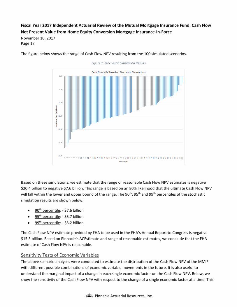
The figure below shows the range of Cash Flow NPV resulting from the 100 simulated scenarios.
Figure 1: Stochastic Simulation Results
Based on these simulations, we estimate that the range of reasonable Cash Flow NPV estimates is negative
$20.4 billion to negative $7.6 billion. This range is based on an 80% likelihood that the ultimate Cash Flow NPV
will fall within the lower and upper bound of the range. The 90th, 95th and 99th percentiles of the stochastic
simulation results are shown below:
90th percentile: ‐ $7.6 billion
95th percentile: ‐ $5.7 billion
99th percentile: ‐ $3.2 billion
The Cash Flow NPV estimate provided by FHA to be used in the FHA’s Annual Report to Congress is negative
$15.5 billion. Based on Pinnacle’s ACEstimate and range of reasonable estimates, we conclude that the FHA
estimate of Cash Flow NPV is reasonable.
Sensitivity Tests of Economic Variables
The above scenario analyses were conducted to estimate the distribution of the Cash Flow NPV of the MMIF
with different possible combinations of economic variable movements in the future. It is also useful to
understand the marginal impact of a change in each single economic factor on the Cash Flow NPV. Below, we
show the sensitivity of the Cash Flow NPV with respect to the change of a single economic factor at a time. This

Fiscal Year 2017 Independent Actuarial Review of the Mutual Mortgage Insurance Fund: Cash Flow
Net Present Value from Home Equity Conversion Mortgage Insurance‐In‐Force November 10, 2017 Page 18
Pinnacle Actuarial Resources, Inc.
sensitivity test is conducted for the House Price Appreciation (HPA) and interest rates.
The marginal impact is measured by the change of the Cash Flow NPV based on the OMB scenario. These
simulations change each of these variables one at a time from the OMB scenario. The changes are parallel shifts
in the path of each variable in the OMB scenario, where all three interest rates are shifted together and at the
same magnitudes, but are kept from going negative.
Figure 2 reports the sensitivity of the Cash Flow NPV with respect to changes in the HPA forecast. Specifically, we applied a parallel shift to the annualized HPA rates from the base scenario up and down by 20, 50, 100 and 200 basis points. The sensitivity to shifts in the
annualized HPA from the base scenario has a positive slope, and a more significant effect from increases in HPAs than decreases. The results show that adverse house price shifts reduce the Cash Flow NPV by a lower level of magnitude than favorable house price shifts increase the Cash Flow NPV. A negative 100 basis points parallel shift in HPA will decrease Cash Flow NPV by $1.3 billion, and a positive
100 basis points parallel shift in HPA will increase Cash Flow NPV by $980 million.
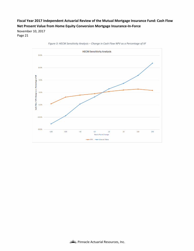
Figure 3 shows the change in Cash Flow NPV as a percentage of the IIF. The change as a percentage of IIF ranges
from ‐4.5% to +1.4%.
Figure 2 also reports the sensitivity of the Cash Flow NPV with respect to changes in interest rates. Specifically, we applied a parallel shift to the annualized CMT and mortgage rates from the base scenario up and down by 20, 50, 100 and 200 basis points. The sensitivity to shifts in the interest rates from the base scenario has a positive slope. A negative 100 basis points parallel shift in interest rates will

Fiscal Year 2017 Independent Actuarial Review of the Mutual Mortgage Insurance Fund: Cash Flow
Net Present Value from Home Equity Conversion Mortgage Insurance‐In‐Force November 10, 2017 Page 19
Pinnacle Actuarial Resources, Inc.
decrease Cash Flow NPV by $6.6 billion, and a positive 100 basis points parallel shift in HPA will increase Cash Flow NPV by $4.9 billion.
Figure 3 shows the change in Cash Flow NPV as a percentage of the IIF. The change as a percentage of IIF ranges
from ‐12.7% to +11.9%.

Fiscal Year 2017 Independent Actuarial Review of the Mutual Mortgage Insurance Fund: Cash Flow
Net Present Value from Home Equity Conversion Mortgage Insurance‐In‐Force November 10, 2017 Page 20
Pinnacle Actuarial Resources, Inc.
Figure 2: HECM Sensitivity Analysis – Change in Cash Flow NPV
Fiscal Year 2017 Independent Actuarial Review of the Mutual Mortgage Insurance Fund: Cash Flow
Net Present Value from Home Equity Conversion Mortgage Insurance‐In‐Force November 10, 2017 Page 21
Pinnacle Actuarial Resources, Inc.
Figure 3: HECM Sensitivity Analysis – Change in Cash Flow NPV as a Percentage of IIF
Fiscal Year 2017 Independent Actuarial Review of the Mutual Mortgage Insurance Fund: Cash Flow
Net Present Value from Home Equity Conversion Mortgage Insurance‐In‐Force November 10, 2017 Page 22
Pinnacle Actuarial Resources, Inc.
Section 4. Summary of Methodology This section describes the analytical approach implemented in this analysis.
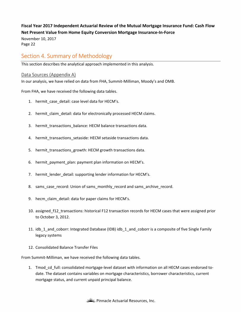
Data Sources (Appendix A)
In our analysis, we have relied on data from FHA, Summit‐Milliman, Moody’s and OMB.
From FHA, we have received the following data tables.
1. hermit_case_detail: case level data for HECM’s.
2. hermit_claim_detail: data for electronically processed HECM claims.
3. hermit_transactions_balance: HECM balance transactions data.
4. hermit_transactions_setaside: HECM setaside transactions data.
5. hermit_transactions_growth: HECM growth transactions data.
6. hermit_payment_plan: payment plan information on HECM’s.
7. hermit_lender_detail: supporting lender information for HECM’s.
8. sams_case_record: Union of sams_monthly_record and sams_archive_record.
9. hecm_claim_detail: data for paper claims for HECM’s.
10. assigned_f12_transactions: historical F12 transaction records for HECM cases that were assigned prior
to October 3, 2012.
11. idb_1_and_coborr: Integrated Database (IDB) idb_1_and_coborr is a composite of five Single Family
legacy systems
12. Consolidated Balance Transfer Files
From Summit‐Milliman, we have received the following data tables.
1. Tmod_cd_full: consolidated mortgage‐level dataset with information on all HECM cases endorsed to‐
date. The dataset contains variables on mortgage characteristics, borrower characteristics, current
mortgage status, and current unpaid principal balance.

Fiscal Year 2017 Independent Actuarial Review of the Mutual Mortgage Insurance Fund: Cash Flow
Net Present Value from Home Equity Conversion Mortgage Insurance‐In‐Force November 10, 2017 Page 23
Pinnacle Actuarial Resources, Inc.
2. Tmod_ti_trans: transaction‐level dataset with tax and insurance delinquency related cash flows over
time for HECM cases.
3. Tmod_upb_fyr_fqtr: dataset with one observation per mortgage‐fiscal quarter with UPB information
over time for each HECM case.
From Moody’s, we have received the following data elements.
1. Historical Economic Data
2. Baseline Economic Scenario Projections
3. Alternative Economic Scenario Projections
From OMB, we received the Economic Assumptions for the 2018 Budget Fall Baseline as of March, 2017
The economic data that is included in the analysis is shown below.
1. HPI
2. Mortgage rates
3. CMT rates
4. LIBOR
Data Processing – Mortgage‐Level Modeling
Starting with the raw data, Pinnacle processed the data to create datasets for developing the mortgage‐level
transition and loss severity models. The steps below describe the data processing that occurred to prepare the
data that was used for this analyses.
1. Pre‐Processing: fields from supplemental tables were added to main HECM Case file
2. HECM Quarterly: a number of calculated fields and flags are added to the dataset
3. Transaction Processing: quarterly historical transactions are then processed
4. Claim Processing: historical claim amounts are calculated based on claims transactions
5. Historical quarterly UPB is calculated for each mortgage
6. MIP Processing: Initial and subsequent MIP inflows are summarized by case number and period from the
Consolidated Balance Transfer File
7. Cash Draw Processing: Incremental and cumulative cash draws are calculated by case number and
period
8. Taxes and Insurance Processing: Incremental and cumulative taxes and insurance are calculated by case
number and period
9. Line of Credit Processing: Incremental and cumulative line of credit draws are calculated by case number
and period
10. Table Joins: tables generated in steps 3 – 9 were joined to the main table created in step 2
Fiscal Year 2017 Independent Actuarial Review of the Mutual Mortgage Insurance Fund: Cash Flow
Net Present Value from Home Equity Conversion Mortgage Insurance‐In‐Force November 10, 2017 Page 24
Pinnacle Actuarial Resources, Inc.
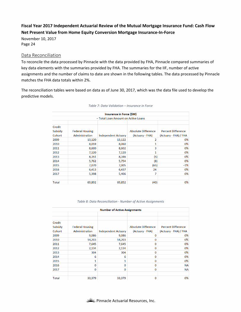
Data Reconciliation
To reconcile the data processed by Pinnacle with the data provided by FHA, Pinnacle compared summaries of
key data elements with the summaries provided by FHA. The summaries for the IIF, number of active
assignments and the number of claims to date are shown in the following tables. The data processed by Pinnacle
matches the FHA data totals within 2%.
The reconciliation tables were based on data as of June 30, 2017, which was the data file used to develop the
predictive models.
Table 7: Data Validation – Insurance in Force
Table 8: Data Reconciliation ‐ Number of Active Assignments

Fiscal Year 2017 Independent Actuarial Review of the Mutual Mortgage Insurance Fund: Cash Flow
Net Present Value from Home Equity Conversion Mortgage Insurance‐In‐Force November 10, 2017 Page 25
Pinnacle Actuarial Resources, Inc.
Table 9: Data Reconciliation – Number of Claims to Date
HECM Base Termination Model (Appendix B)
Pinnacle developed predictive models to estimate future HECM terminations. No repayment of principal is
required on a HECM while the mortgage is active. Termination of a HECM typically occurs due to death of the
borrower, the borrower moving out, or voluntary termination via refinance or payoff. The termination model
estimates the probabilities of the three mutually exclusive HECM termination events denoted as mortality,
mobility and refinance. A multinomial logistic regression modeling approach was used to analyze the different
termination events.
The termination model incorporates four main categories of explanatory variables:
Fixed initial borrower characteristics, such as borrower age at origination and gender.
Fixed initial mortgage characteristics, such as mortgage interest rate, origination year and quarter, the
first month cash draw percentage, the estimated ratio of the property value to the local area’s median
home values at time of origination, and the estimated ratio of the local area’s median home value to the
HECM national mortgage limit at the time of origination.
Dynamic variables based on mortgage/borrower characteristics, such as mortgage age and borrower
and co‐borrower ages.
Dynamic variables derived by combining mortgage characteristics with external macroeconomic data,
such as interest rates, HPI, the amount of additional equity available to the borrower through
refinancing and the updated ratio of UPB to home value.
For each possible termination event type, a multinomial logistic model is developed based on mortgage‐level
historical HECM performance data and economic factors to determine the overall termination probabilities for
the HECM’s.

Fiscal Year 2017 Independent Actuarial Review of the Mutual Mortgage Insurance Fund: Cash Flow
Net Present Value from Home Equity Conversion Mortgage Insurance‐In‐Force November 10, 2017 Page 26
Pinnacle Actuarial Resources, Inc.
HECM Cash Flow Draw Projection Models (Appendix C)
Over 90% of HECM’s have a line of credit associated with them. To estimate the present value of future cash
flows on the existing portfolio of HECM’s, we need to estimate the future cash draws associated with the line of
credit. As these cash draws are not certain as they would be for a term product, we have developed predictive
models to forecast cash draws. We have incorporated a two‐stage model:
1. A binomial model is developed to estimate the likelihood of a cash draw occurring in a period
2. A Generalized Linear Model (GLM) is then developed to estimate the amount of the cash draw for the
period
Using the historical HECM data, for each quarter we develop an indicator of whether or not a net positive
unscheduled cash draw was taken from the line of credit during that quarter, and also the amount of the cash
draw. We then develop models to predict the amount of future cash draws based on a series of explanatory
variables. The explanatory variables used in the model are the same as those used for the Base Termination
Models.
HECM Cash Flow Analysis (Appendix E)
HECM termination rates are projected for all future policy years for each active mortgage. The variables used in
the projection are derived from mortgage characteristics and economic forecasts. Moody’s September 2017
forecasts of interest, unemployment rates and HPI are combined with the mortgage‐level data to simulate the
projected economic paths and create the necessary forecasted variables. MSA‐level forecasts of HPI apply to
mortgages in metropolitan areas; otherwise mortgages use the state‐level HPI forecasts. Moody’s house price
forecasts are generated simultaneously with various macroeconomic variables including the local
unemployment rates.
For each mortgage during future policy years, the derived mortgage variables serve as independent variables to
the multinomial logistic termination models described in the Base Termination Model section. The termination
projections by claim type are then calculated to generate the probability of mortgage termination in a policy
year by different modes of termination given that it survives to the end of the prior policy year. The HECM cash
flow model uses these forecasted termination rates to project the cash flows associated with different
termination events. Based on the specific characteristics of the mortgage, the probability of each termination is
calculated. Then, a random number between 0 and 1 is generated, and based on this random draw a mortgage
transition is determined. The projection process continues for each mortgage until the mortgage ends by
termination or claim.
Cash Flow Components
There are four major components of HECM cash flows:
1. MIP,
2. claims,
Fiscal Year 2017 Independent Actuarial Review of the Mutual Mortgage Insurance Fund: Cash Flow
Net Present Value from Home Equity Conversion Mortgage Insurance‐In‐Force November 10, 2017 Page 27
Pinnacle Actuarial Resources, Inc.
3. note holding expenses, and
4. recoveries on notes in inventory (after assignment).
Premiums consist of upfront and annual MIPs, which are inflows to the HECM program. Recoveries are the
property recovery amount received by FHA at the time of note termination after assignment, which is the
minimum of the mortgage balance and the predicted net sales proceeds at termination. The recovery amount
for refinance termination is always the mortgage balance. Claim Type 1 payments are cash outflows paid to the
lender when the net proceeds of a property sale are insufficient to cover the balance of the mortgage. Claim
Type 2 payments result from assignment of mortgages to HUD and note holding payments are additional
outflows.
Net Future Cash Flows
The Cash Flow NPV for the HECM book of business is computed by summing the individual components as they
occur over time:
Net Cash Flowt = Annual Premiumst + Recoveriest ‐ Claim Type 1t ‐ Claim Type 2t ‐ Note Holding Expensest
Discount Factors
The discount factors applied were provided by FHA and reflect the most recent Treasury yield curve, which
captures the Federal government’s cost of capital in raising funds. These factors reflect the capital market’s
expectation of the consolidated interest risk of U.S. Treasury securities. Our simulations aggregated each future
quarter’s cash flows, which are treated as being received at the end of the quarter.
Fiscal Year 2017 Independent Actuarial Review of the Mutual Mortgage Insurance Fund: Cash Flow
Net Present Value from Home Equity Conversion Mortgage Insurance‐In‐Force November 10, 2017 Page 28
Pinnacle Actuarial Resources, Inc.
Appendices
A. Data Sources, Processing and Reconciliation
B. HECM Base Termination Model
C. HECM Cash Flow Draw Projection Model
D. Economic Scenarios
E. HECM Cash Flow Analysis

Fiscal Year 2017 Independent Actuarial Review of the Mutual Mortgage Insurance Fund: Cash Flow
Net Present Value from Home Equity Conversion Mortgage Insurance‐In‐Force November 10, 2017 Page 29
Pinnacle Actuarial Resources, Inc.
Appendix A: Data Sources, Processing and Reconciliation In our analysis, we have relied on data from FHA, Summit‐Milliman, Moody’s and OMB.
From FHA, we have received the following data tables.
1. hermit_case_detail: case level data for HECM mortgages.
2. hermit_claim_detail: data for electronically processed HECM claims.
3. hermit_transactions_balance: HECM balance transactions data.
4. hermit_transactions_setaside: HECM setaside transactions data.
5. hermit_transactions_growth: HECM growth transactions data.
6. hermit_payment_plan: payment plan information on HECM mortgages.
7. hermit_lender_detail: supporting lender information for HECM mortgages.
8. sams_case_record: Union of sams_monthly_record and sams_archive_record.
9. hecm_claim_detail: data for paper claims for HECM mortgages.
10. assigned_f12_transactions: historical F12 transaction records for HECM cases that were assigned prior
to October 3, 2012.
11. idb_1_and_coborr: Integrated Database (IDB) idb_1_and_coborr is a composite of five Single Family
legacy systems
12. Consolidated Balance Transfer Files
From Summit‐Milliman, we have received the following data tables.
1. Tmod_cd_full: consolidated mortgage‐level dataset with information on all HECM cases endorsed to‐
date. The dataset contains variables on mortgage characteristics, borrower characteristics, current
mortgage status, and current unpaid principal balance.
2. Tmod_ti_trans: transaction‐level dataset with tax and insurance delinquency related cash flows over
time for HECM cases.

Fiscal Year 2017 Independent Actuarial Review of the Mutual Mortgage Insurance Fund: Cash Flow
Net Present Value from Home Equity Conversion Mortgage Insurance‐In‐Force November 10, 2017 Page 30
Pinnacle Actuarial Resources, Inc.
3. Tmod_upb_fyr_fqtr: dataset with one observation per mortgage‐fiscal quarter with UPB information
over time for each HECM case.
From Moody’s, we have received the following data elements.
1. Historical Economic Data
2. Baseline Economic Scenario Projections
3. Alternative Economic Scenario Projections
From OMB, we received the Economic Assumptions for the 2018 Budget Fall Baseline as of March, 2017.
The economic data that is included in the analysis is shown below.
1. HPI
2. Mortgage rates
3. CMT rates
4. LIBOR
Data Processing – Mortgage Level Modeling
Beginning with the data tables provided by FHA, the data was processed to create datasets for developing the
mortgage level transition and cash draw models. The steps below describe the data processing that occurred to
prepare the data that was used for these analyses.
1. Pre‐Processing: fields from supplemental tables were added to main HECM Case file
2. HECM Quarterly: a number of calculated fields and flags are added to the dataset
3. Transaction Processing: quarterly historical transactions are then processed
4. Claim Processing: historical claim amounts are calculated based on claims transactions
5. Historical quarterly UPB is calculated for each mortgage
6. MIP Processing: Initial and subsequent MIP inflows are summarized by case number and period from the
Consolidated Balance Transfer File
7. Cash Draw Processing: Incremental and cumulative cash draws are calculated by case number and
period
8. Taxes and Insurance Processing: Incremental and cumulative taxes and insurance are calculated by case
number and period
9. Line of Credit Processing: Incremental and cumulative line of credit draws are calculated by case number
and period
10. Table Joins: tables generated in steps 3 – 9 were joined to the main table created in step 2
Data Reconciliation
To reconcile the data processed by Pinnacle with the data provided by FHA, Pinnacle compared summaries of
key data elements with the summaries provided by FHA. The summaries for the IIF, number of active
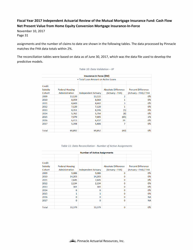
Fiscal Year 2017 Independent Actuarial Review of the Mutual Mortgage Insurance Fund: Cash Flow
Net Present Value from Home Equity Conversion Mortgage Insurance‐In‐Force November 10, 2017 Page 31
Pinnacle Actuarial Resources, Inc.
assignments and the number of claims to date are shown in the following tables. The data processed by Pinnacle
matches the FHA data totals within 2%.
The reconciliation tables were based on data as of June 30, 2017, which was the data file used to develop the
predictive models.
Table 10: Data Validation – IIF
Table 11: Data Reconciliation ‐ Number of Active Assignments

Fiscal Year 2017 Independent Actuarial Review of the Mutual Mortgage Insurance Fund: Cash Flow
Net Present Value from Home Equity Conversion Mortgage Insurance‐In‐Force November 10, 2017 Page 32
Pinnacle Actuarial Resources, Inc.
Table 12: Data Reconciliation – Number of Claims to Date
Fiscal Year 2017 Independent Actuarial Review of the Mutual Mortgage Insurance Fund: Cash Flow
Net Present Value from Home Equity Conversion Mortgage Insurance‐In‐Force November 10, 2017 Page 33
Pinnacle Actuarial Resources, Inc.
Appendix B: HECM Base Termination Model HECM mortgages terminate due to borrower mortality (death), the borrowers refinancing the mortgage or the
borrower moving out (mobility). A multinomial logistic model is specified and estimated to capture the
mortgage termination behavior.
The available FHA historical HECM termination data was used to develop the base termination model. This data
includes mortgages that were endorsed under the GI Fund between fiscal years 1990 and 2008, and mortgages
endorsed under the MMIF from fiscal year 2009 through September 30, 2017. Only mortgages endorsed under
the MMIF, however, are used in the calculation of the Cash Flow NPV in this analysis.
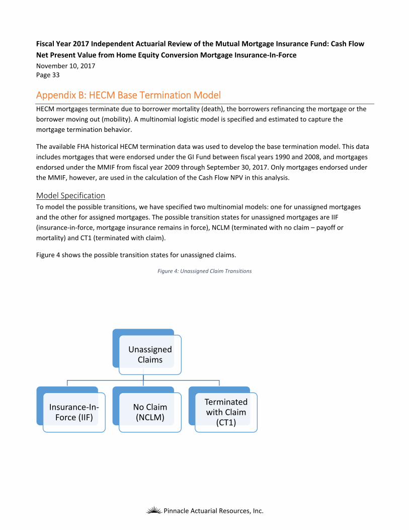
Model Specification
To model the possible transitions, we have specified two multinomial models: one for unassigned mortgages
and the other for assigned mortgages. The possible transition states for unassigned mortgages are IIF
(insurance‐in‐force, mortgage insurance remains in force), NCLM (terminated with no claim – payoff or
mortality) and CT1 (terminated with claim).
Figure 4 shows the possible transition states for unassigned claims.
Figure 4: Unassigned Claim Transitions
Unassigned Claims
Insurance‐In‐Force (IIF)
No Claim (NCLM)
Terminated with Claim
(CT1)

Fiscal Year 2017 Independent Actuarial Review of the Mutual Mortgage Insurance Fund: Cash Flow
Net Present Value from Home Equity Conversion Mortgage Insurance‐In‐Force November 10, 2017 Page 34
Pinnacle Actuarial Resources, Inc.
For assigned claims, the possible transition states are CT2a (remains active and assigned), CT2p (terminated with
payoff), and CT2c (terminated with conveyance). Figure 5 shows the possible transition states for assigned
claims.
Figure 5: Assigned Claim Transitions
Multinomial Logistic Regression Theory
Multinomial logistic regression is used to model the relationship between a collection of predictor variables and
the distributional behavior of a polytomous response variable. It is a likelihood‐based methodology and may be
viewed as the generalization of logistic regression for a response variable with more than two levels.
To formalize its description, let the response variable Y take m possible levels, denoted for simplicity as 1,…,m,
and assume there is a collection of g predictors, X ,…, X , that is used to model Y’s distribution. We assume that
Y and X ,…, X are jointly observed n times with the ith random observation being labeled as
Y , X ,…, X and its realized value y , x ,…, x .
In a multinomial logistic regression, the mathematical structure of the model is set by the following two
assumptions:
1. The g+1 length random vectors <Y , X ,…, X > are jointly independent across all i
2. Given that X ,…, X have been observed at x ,…, x , Y ’s distribution is assumed to be multinomial
with
P(Y = l) = exp( +∑ ∙x )/(∑ exp( +∑ ∙x )) ,
Assigned Claims
Remains Active and Assigned
(CT2a)
Terminated with Payoff (CT2p)
Terminated with Conveyance
(CT2c)

Fiscal Year 2017 Independent Actuarial Review of the Mutual Mortgage Insurance Fund: Cash Flow
Net Present Value from Home Equity Conversion Mortgage Insurance‐In‐Force November 10, 2017 Page 35
Pinnacle Actuarial Resources, Inc.
where the are unknown regression parameters and the j are unknown intercept parameters. [Note:
To prevent over‐specification of the model due to the constraint that the above probabilities sum to 1
over l=1,…,m, a base level j is chosen such that and are set equal to zero.] Thus, if j = 1, then
P(Y =1) = 1/(1 ∑ exp( +∑ ∙x )) .
It now follows the likelihood equation for this model is given by
∏ P(Y =y ) = ∏ exp( +∑ ∙x )/(∑ exp( +∑ ∙x )).
The multinomial logistic regression procedure optimizes the above likelihood over the unknown parameters in
order to find those parameters that, in some sense, are most likely to have given rise to the data.
The target variables for the unassigned and assigned transition models are shown above in Figure 4 and Figure 5.
The independent variables used in the models are described in the next section. The models were developed
using a traditional train/test/validate approach. A random sample of the data is used to train the multinomial
model, and a second random sample is used to test and refine the model parameters and to determine inclusion
and exclusion of explanatory variables. The third random sample, the validation data, is used as a final validation
step to test the predictive power of the final model.
To generate the random sample, random numbers were added to the dataset at the case level using a random
number generator. The random numbers were drawn from a uniform distribution between 0 and 1. Based on
these random numbers, 40% of the cases were assigned to the train dataset, 30% were assigned to the test
dataset and 30% were assigned to the validation dataset.
Explanatory Variables
The following explanatory variables are used in the transition models for assigned and unassigned claims.
Period number: this is the number of quarters since the inception of the mortgage. In the transition
models, period number enters as a fourth degree polynomial.
Remaining line of credit: this is the amount of the line of credit that still remains to be drawn. Remaining
line of credit enters the models as a fourth degree polynomial.
Gross Domestic Product (GDP): the change in the gross domestic product over the period the mortgage
has been in effect is included in the model. GDP enters the models as a fourth degree polynomial.
Refinance Incentive: the incentive to refinance increases as the difference between current interest and
the prevailing market rate increases. We have included this effect as the ratio of the current mortgage
interest rate to the 1‐Year Treasury Rate (refi = int_rt / 1‐Year Treasury Rate). The first four powers of
this this variable were included in the model.

Fiscal Year 2017 Independent Actuarial Review of the Mutual Mortgage Insurance Fund: Cash Flow
Net Present Value from Home Equity Conversion Mortgage Insurance‐In‐Force November 10, 2017 Page 36
Pinnacle Actuarial Resources, Inc.
The number of borrowers and co‐borrowers that are alive
The youngest age amongst the borrower and co‐borrowers
The interest rate type (annual adjustable, monthly adjustable or fixed)
The gender of the borrower and co‐borrower
City/state grouping
The initial PL is normalized in the models, and is included as initial_principal_limit/100,000
Whether a mortgage was a part of the HECM saver program
The log of the unemployment rate
Model Validation
Model validation was accomplished by applying the models developed using the training set to the validation
dataset. The application of this model to the validation data produces the probability of each transition type for
the unassigned claim model and the assigned claim model. The actual target variable is then compared to the
predicted target variable to ensure the model fits the transition process without over‐fitting the actual data.
Specifically we calculate the predicted probability of the each transition (for the unassigned model) or the claim
type (for the assigned claim model). The actual result is 1.0 for the final transition and claim type and 0.0 for all
other transition or claim types. The probability of each transition or claim type for each record in the validation
dataset is derived from the model parameters. The sum of the predicted probabilities is 1.0 for each record.
Decile charts are then created for each final unassigned transition or assigned claim type. All records are sorted,
or ranked, by the predicted value. Ten equal sized decile groups are created with 10% of the records in each
group. The sum of the actual result and the sum of the predicted result within each decile is calculated. The
actual and predicted numbers are then compared for consistency. The objective of a model is to have a
significant spread in predicted values while maintaining a close relationship between the resulting actual and
predicted values.
The validation chart for the unassigned claim models with an ending condition of IIF is shown below.
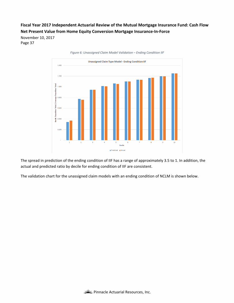
Fiscal Year 2017 Independent Actuarial Review of the Mutual Mortgage Insurance Fund: Cash Flow
Net Present Value from Home Equity Conversion Mortgage Insurance‐In‐Force November 10, 2017 Page 37
Pinnacle Actuarial Resources, Inc.
Figure 6: Unassigned Claim Model Validation – Ending Condition IIF
The spread in prediction of the ending condition of IIF has a range of approximately 3.5 to 1. In addition, the
actual and predicted ratio by decile for ending condition of IIF are consistent.
The validation chart for the unassigned claim models with an ending condition of NCLM is shown below.

Fiscal Year 2017 Independent Actuarial Review of the Mutual Mortgage Insurance Fund: Cash Flow
Net Present Value from Home Equity Conversion Mortgage Insurance‐In‐Force November 10, 2017 Page 38
Pinnacle Actuarial Resources, Inc.
Figure 7: Unassigned Claim Model Validation – Ending Condition NCLM
The spread in prediction of the ending condition of NCLM has a range of approximately 10 to 1. In addition, the
actual and predicted ratio by decile for ending condition of NCLM are consistent.
The validation chart for the unassigned claim models with an ending condition of CT1 is shown below.

Fiscal Year 2017 Independent Actuarial Review of the Mutual Mortgage Insurance Fund: Cash Flow
Net Present Value from Home Equity Conversion Mortgage Insurance‐In‐Force November 10, 2017 Page 39
Pinnacle Actuarial Resources, Inc.
Figure 8: Unassigned Claim Model Validation – Ending Condition CT1
The number of CT1 claims in the historical data is relatively small, so the validation results are volatile. However,
there is a significant spread in segmentation between deciles, and there is a consistent relationship between the
actual and predicted transitions by decile also.
The validation chart for the assigned claim models with an ending condition of CT2a is shown below.
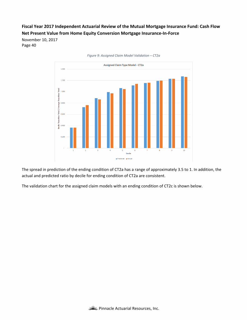
Fiscal Year 2017 Independent Actuarial Review of the Mutual Mortgage Insurance Fund: Cash Flow
Net Present Value from Home Equity Conversion Mortgage Insurance‐In‐Force November 10, 2017 Page 40
Pinnacle Actuarial Resources, Inc.
Figure 9: Assigned Claim Model Validation – CT2a
The spread in prediction of the ending condition of CT2a has a range of approximately 3.5 to 1. In addition, the
actual and predicted ratio by decile for ending condition of CT2a are consistent.
The validation chart for the assigned claim models with an ending condition of CT2c is shown below.

Fiscal Year 2017 Independent Actuarial Review of the Mutual Mortgage Insurance Fund: Cash Flow
Net Present Value from Home Equity Conversion Mortgage Insurance‐In‐Force November 10, 2017 Page 41
Pinnacle Actuarial Resources, Inc.
Figure 10: Assigned Claim Model Validation – CT2c
The spread in prediction of the ending condition of CT2c has a range of approximately 40 to 1. In addition, the
actual and predicted ratio by decile for ending condition of CT2c are consistent.
The validation chart for the assigned claim models with an ending condition of CT2p is shown below.

Fiscal Year 2017 Independent Actuarial Review of the Mutual Mortgage Insurance Fund: Cash Flow
Net Present Value from Home Equity Conversion Mortgage Insurance‐In‐Force November 10, 2017 Page 42
Pinnacle Actuarial Resources, Inc.
Figure 11: Assigned Claim Model Validation – CT2p
The spread in prediction of the ending condition of CT2c has a range of approximately 17 to 1. In addition, the
actual and predicted ratio by decile for ending condition of CT2c are consistent.

Fiscal Year 2017 Independent Actuarial Review of the Mutual Mortgage Insurance Fund: Cash Flow
Net Present Value from Home Equity Conversion Mortgage Insurance‐In‐Force November 10, 2017 Page 43
Pinnacle Actuarial Resources, Inc.
Appendix C: HECM Cash Draw Projection Models Over 90% of HECM‘s have a line of credit associated with them. To estimate the Cash Flow NPV on the existing
portfolio of HECM mortgages, we need to estimate the future unscheduled cash draws associated with
mortgages with a line of credit. As these cash draws are not certain, we have developed predictive models to
forecast unscheduled cash draws for HECM with a line of credit. We have incorporated a two‐stage model:
1. A binomial model is developed to estimate the likelihood of a cash draw occurring in a period
2. A GLM is then developed to estimate the amount of the cash draw for the period
Likelihood of a Cash Draw
For the historical HECM database, for each quarter we develop an indicator of whether or not a net positive
unscheduled cash draw was taken from the line of credit during that quarter. We then developed a binomial
logistic model to estimate the likelihood of an unscheduled cash draw occurring during the quarter based on a
series of explanatory variables. The explanatory variables used in the model are the same as those used for the
Base Termination Models. These variables are described in Appendix B.
Separate models were developed for mortgage type 2 (Line of Credit) and mortgage types 4 and 5 (Term Plus
Line of Credit and Tenure Plus Line of Credit).
Estimated Cash Draw Amount
For the estimated cash draw amount, we developed a model using the Incremental Line of Credit Cash Draw
from the historical HECM database. This incremental cash draw was used as the target variable, and we
estimated the predicted amount of the cash draw based on a series of explanatory variables. The explanatory
variables used in the model are the same as those used for the Base Termination Models. These variables are
described in Appendix B.
We used a GLM to predict the cash draw, specifying a Gamma Error structure and a log link function. We also
developed separate models for mortgage type 2 (Line of Credit) and mortgage types 4 and 5 (Term Plus Line of
Credit and Tenure Plus Line of Credit).
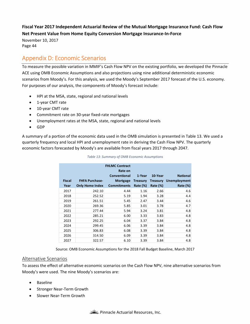
Fiscal Year 2017 Independent Actuarial Review of the Mutual Mortgage Insurance Fund: Cash Flow
Net Present Value from Home Equity Conversion Mortgage Insurance‐In‐Force November 10, 2017 Page 44
Pinnacle Actuarial Resources, Inc.
Appendix D: Economic Scenarios To measure the possible variation in MMIF’s Cash Flow NPV on the existing portfolio, we developed the Pinnacle
ACE using OMB Economic Assumptions and also projections using nine additional deterministic economic
scenarios from Moody’s. For this analysis, we used the Moody’s September 2017 forecast of the U.S. economy.
For purposes of our analysis, the components of Moody’s forecast include:
HPI at the MSA, state, regional and national levels
1‐year CMT rate
10‐year CMT rate
Commitment rate on 30‐year fixed‐rate mortgages
Unemployment rates at the MSA, state, regional and national levels
GDP
A summary of a portion of the economic data used in the OMB simulation is presented in Table 13. We used a
quarterly frequency and local HPI and unemployment rate in deriving the Cash Flow NPV. The quarterly
economic factors forecasted by Moody’s are available from fiscal years 2017 through 2047.
Table 13: Summary of OMB Economic Assumptions
Source: OMB Economic Assumptions for the 2018 Fall Budget Baseline, March 2017
Alternative Scenarios
To assess the effect of alternative economic scenarios on the Cash Flow NPV, nine alternative scenarios from
Moody’s were used. The nine Moody’s scenarios are:
Baseline
Stronger Near‐Term Growth
Slower Near‐Term Growth
Fiscal
Year
FHFA Purchase‐
Only Home Index
FHLMC Contract
Rate on
Conventional
Mortgage
Commitments
1‐Year
Treasury
Rate (%)
10‐Year
Treasury
Rate (%)
National
Unemployment
Rate (%)
2017 242.10 4.44 1.16 2.66 4.6
2018 252.52 5.19 1.94 3.28 4.4
2019 261.51 5.45 2.47 3.44 4.6
2020 269.36 5.85 3.01 3.78 4.7
2021 277.44 5.94 3.24 3.81 4.8
2022 285.21 6.00 3.33 3.83 4.8
2023 292.25 6.04 3.37 3.84 4.8
2024 299.45 6.06 3.39 3.84 4.8
2025 306.83 6.08 3.39 3.84 4.8
2026 314.50 6.09 3.39 3.84 4.8
2027 322.57 6.10 3.39 3.84 4.8

Fiscal Year 2017 Independent Actuarial Review of the Mutual Mortgage Insurance Fund: Cash Flow
Net Present Value from Home Equity Conversion Mortgage Insurance‐In‐Force November 10, 2017 Page 45
Pinnacle Actuarial Resources, Inc.
Moderate Recession
Protracted Slump
Below‐Trend Long‐Term Growth
Stagflation
Next‐Cycle Recession
Low Oil Price
The Moody’s projections provide a range of better than expected economic assumptions and worse than
expected economic assumptions. This range of assumptions produces a range of Cash Flow NPV projections.
Graphical Depiction of the Scenarios
Figure 12 shows the future movements of the HPI under the baseline and the alternative economic scenarios.
For the OMB projections, the HPI increases as a fairly steady rate throughout the entire projection period. For
the Moody’s Baseline Scenario, the HPI appreciation rate increases at a slower rate through 2022, at which time
the rate of increase becomes greater than the OMB rate. The Moody’s Baseline HPI projection is higher than the
OMB baseline after 2024.
Figure 12: Paths of the Future National House Price Index in Different Scenarios
Figure 13 shows the forecasted mortgage rate of 30‐year fixed‐rate mortgages for the nine scenarios. OMB’s
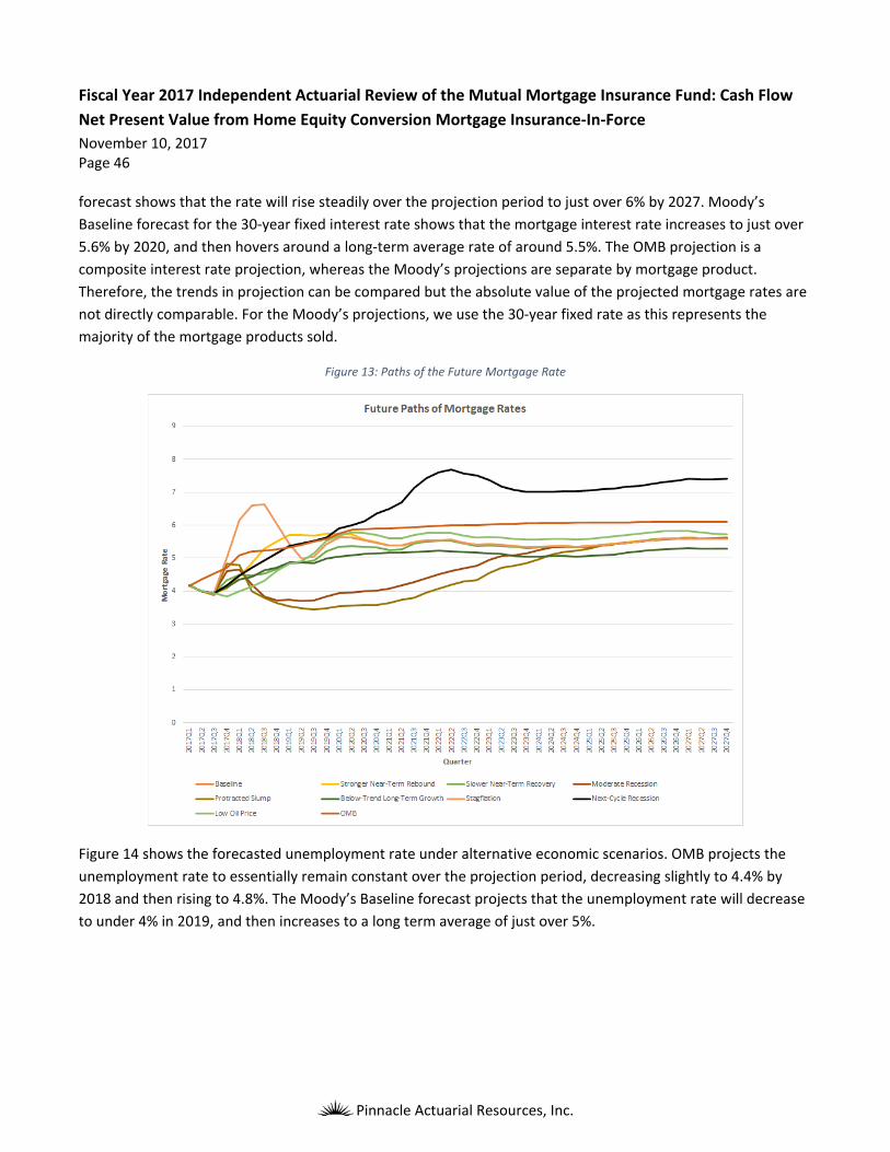
Fiscal Year 2017 Independent Actuarial Review of the Mutual Mortgage Insurance Fund: Cash Flow
Net Present Value from Home Equity Conversion Mortgage Insurance‐In‐Force November 10, 2017 Page 46
Pinnacle Actuarial Resources, Inc.
forecast shows that the rate will rise steadily over the projection period to just over 6% by 2027. Moody’s
Baseline forecast for the 30‐year fixed interest rate shows that the mortgage interest rate increases to just over
5.6% by 2020, and then hovers around a long‐term average rate of around 5.5%. The OMB projection is a
composite interest rate projection, whereas the Moody’s projections are separate by mortgage product.
Therefore, the trends in projection can be compared but the absolute value of the projected mortgage rates are
not directly comparable. For the Moody’s projections, we use the 30‐year fixed rate as this represents the
majority of the mortgage products sold.
Figure 13: Paths of the Future Mortgage Rate
Figure 14 shows the forecasted unemployment rate under alternative economic scenarios. OMB projects the
unemployment rate to essentially remain constant over the projection period, decreasing slightly to 4.4% by
2018 and then rising to 4.8%. The Moody’s Baseline forecast projects that the unemployment rate will decrease
to under 4% in 2019, and then increases to a long term average of just over 5%.

Fiscal Year 2017 Independent Actuarial Review of the Mutual Mortgage Insurance Fund: Cash Flow
Net Present Value from Home Equity Conversion Mortgage Insurance‐In‐Force November 10, 2017 Page 47
Pinnacle Actuarial Resources, Inc.
Figure 14: Paths of Future National Unemployment Rate
Stochastic Simulations
This section describes the stochastic models which we fit to generate the economic variables simulations used in
the analysis of the HECM Portfolio.
The modeled economic variables include:
1‐Year CMT Rates
3‐Month CMT Rates
6‐Month CMT Rates
2‐Year CMT Rates
3‐Year CMT Rates
5‐Year CMT Rates
7‐Year CMT Rates
10‐Year CMT Rates
20‐Year CMT Rates
30‐Year CMT Rates
30‐Year Fixed Rate Mortgage (FRM) Rates
FHFA National Purchase Only House Price Index (HPI‐PO)

Fiscal Year 2017 Independent Actuarial Review of the Mutual Mortgage Insurance Fund: Cash Flow
Net Present Value from Home Equity Conversion Mortgage Insurance‐In‐Force November 10, 2017 Page 48
Pinnacle Actuarial Resources, Inc.
Unemployment Rates
GDP
Historical Data
A. Interest Rates
Figure 15 shows historical interest rates since the first quarter of 1971.
This graph illustrates the variability of interest rates over time and the consistent spread between rates. Shown
are the 1‐year CMT rate (tr1y), 10‐year CMT rate (tr10y) and the 30‐year FRM rate (mr).
High inflation rates caused by the global oil crisis in the late 1970’s were the major cause for the historically high
level of interest rates in early 1980’s. The Federal Reserve shifted its monetary policy from managing interest
rates to managing the money supply as a way to influence interest rates after this period of time. The 1‐year
CMT rate was around 5% in calendar year (CY) 1971 and increased steadily to its peak of 16.31% in the third
quarter of CY 1981. Subsequently, the 1‐year CMT rate followed a decreasing trend and reached an all‐time low
of 0.10% in the second quarter of 2014. Since then, rates have started a slow upward trend.
Figure 15: Historical Interest Rates (%)
Figure 16 shows historical interest rate spreads, including the spread between 10‐year and 1‐year CMT rates
(tr10y_s) and the spread between the 30‐year mortgage rate and the 10‐year CMT rate (mr10y_s). Both spreads
have positive values for most of the historical periods with long cycles. Small positive and negative spreads
typically correspond with economic downturns, such as those that occurred during the late 1970’s through early

Fiscal Year 2017 Independent Actuarial Review of the Mutual Mortgage Insurance Fund: Cash Flow
Net Present Value from Home Equity Conversion Mortgage Insurance‐In‐Force November 10, 2017 Page 49
Pinnacle Actuarial Resources, Inc.
1980’s. The spread of the mortgage rate over the 10‐year CMT rate is always positive, reflecting the premium for
credit risk.
Figure 16: Historical Interest Rate Spreads (%)
B. House Price Appreciation Rates
The national HPA rate is derived from the FHFA repeat sales HPI of purchase‐only (PO) transactions. The PO HPI
provides a reliable measure of housing market conditions, since it is based on repeat sales at market prices and
does not use any appraised values.
The HPA series being modeled is defined as:
ln (1)
Figure 17 shows the national quarterly HPA from CY 1971 Q1 to CY 2016 Q4. The long‐term average quarterly
HPA is approximately 0.83% (an annual rate of 3.30%).

Fiscal Year 2017 Independent Actuarial Review of the Mutual Mortgage Insurance Fund: Cash Flow
Net Present Value from Home Equity Conversion Mortgage Insurance‐In‐Force November 10, 2017 Page 50
Pinnacle Actuarial Resources, Inc.
Figure 17: Historical Quarterly HPA
The HPA increased steadily before 2004, and the quarterly appreciation rate was 1.13%. Subsequently, house
prices rose sharply starting in 2004. The average quarterly house price appreciation rate was 1.87% during the
subprime mortgage expansion period from 2004 to 2006, and reached its peak of 2.59% in the second quarter of
CY 2005. After 2006, the average growth rate of house price became negative until 2011, when appreciation
returned to a positive value. Table 14 shows the quarterly HPA by selected historical time periods.
Table 14: Average Quarterly HPA by Time Span
Period Average Quarterly HPA
1991 – 2003 1.13%
2004 – 2006 1.87%
2007 – 2010 ‐1.23%
2011 – 2017 1.03%
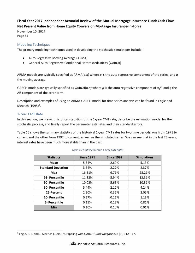
Fiscal Year 2017 Independent Actuarial Review of the Mutual Mortgage Insurance Fund: Cash Flow
Net Present Value from Home Equity Conversion Mortgage Insurance‐In‐Force November 10, 2017 Page 51
Pinnacle Actuarial Resources, Inc.
Modeling Techniques
The primary modeling techniques used in developing the stochastic simulations include:
Auto Regressive Moving Average (ARMA)
General Auto Regressive Conditional Heteroscedasticity (GARCH)
ARMA models are typically specified as ARMA(p,q) where p is the auto regressive component of the series, and q
the moving average.
GARCH models are typically specified as GARCH(p,q) where p is the auto regressive component of , and q the
AR component of the error term.
Description and examples of using an ARMA‐GARCH model for time series analysis can be found in Engle and
Mezrich (1995)3.
1‐Year CMT Rate
In this section, we present historical statistics for the 1‐year CMT rate, describe the estimation model for the
stochastic process, and finally report the parameter estimates and their standard errors.
Table 15 shows the summary statistics of the historical 1‐year CMT rates for two time periods, one from 1971 to
current and the other from 1992 to current, as well as the simulated series. We can see that in the last 25 years,
interest rates have been much more stable than in the past.
Table 15: Statistics for the 1‐Year CMT Rates
Statistics Since 1971 Since 1992 Simulations
Mean 5.34% 2.69% 5.13%
Standard Deviation 3.64% 2.27% 2.37%
Max 16.31% 6.71% 28.21%
95‐ Percentile 11.83% 5.94% 12.31%
90‐ Percentile 10.02% 5.66% 10.31%
50‐ Percentile 5.44% 2.12% 4.24%
25‐Percent 2.30% 0.36% 2.05%
10‐ Percentile 0.27% 0.15% 1.13%
5‐ Percentile 0.15% 0.12% 0.81%
Min 0.10% 0.10% 0.01%
3 Engle, R. F. and J. Mezrich (1995), “Grappling with GARCH”, Risk Magazine, 8 (9), 112 – 17.

Fiscal Year 2017 Independent Actuarial Review of the Mutual Mortgage Insurance Fund: Cash Flow
Net Present Value from Home Equity Conversion Mortgage Insurance‐In‐Force November 10, 2017 Page 52
Pinnacle Actuarial Resources, Inc.
An ARMA(2,4) parameterization was used to model the 1‐Year CMT rate (r1) difference from the previous
period. The model was estimated using data from the first quarter of CY 1971 to the third quarter of CY 2017.
The process takes the following form:
, , , , , , , (2)
Z1 is an independent Wiener random process with distribution N(0,1), and the variance (σ) of the residual term
follows a GARCH(1,1) process:
(3)
ε is the error term, which equals from equation (2).
The Full Information Maximum Likelihood (FIML) method was used to estimate the parameters in equations (2)
and (3). The results are presented in Table 16.
Table 16: Estimation Results for 1‐Year CMT Rate Model
Parameter Estimate Std Dev t‐value prob>t µ 0.0003 0.0002 1.4052 0.1600 x1 0.0424 1.5880 0.0267 0.9787 x2 0.3361 1.3910 0.2416 0.8091 x3 0.3517 1.5558 0.2261 0.8212 x4 ‐0.4119 0.7487 ‐0.5502 0.5822 x4 0.1358 0.4423 0.3070 0.7589 x5 0.3051 0.3723 0.8195 0.4125
β0 0.0000 0.0000 0.0110 0.9912 β1 0.3094 0.0512 6.0382 0.0000 β2 0.6896 0.0424 16.2677 0.0000
Pearson’s Goodness
of Fit 0.9380
The model based on these parameters is used to simulate the 1‐year CMT rates for the forecast period starting
in the fourth quarter of FY 2017. The model fit was evaluated using Akaike Information Criterion (AIC) and
Pearson’s goodness‐of‐fit test.
A lower bound of 0.01 percent was applied to the simulated future 1‐year CMT rates to avoid negative rates in
the simulation.

Fiscal Year 2017 Independent Actuarial Review of the Mutual Mortgage Insurance Fund: Cash Flow
Net Present Value from Home Equity Conversion Mortgage Insurance‐In‐Force November 10, 2017 Page 53
Pinnacle Actuarial Resources, Inc.
Additional Interest Rate Models
Additional models were developed to simulate the other interest rates. All models were estimated as a spread (difference) between the current maturity length and prior. Table 17 describes these spreads and models.
Table 17: Model Specification for Additional Interest Rates
Variable Variable Transformation Model Specification Notes
3‐month AR(1)‐GARCH(1,1)
6‐month ARMA(3,1)‐ARCH(1)
1‐year ARMA(2,4)‐GARCH(1,1) Base Interest Rate
2‐year AR(1)‐ARCH(1)
3‐year ARMA(2,1)‐ARCH(1)
5‐year ARMA(2,1)‐ARCH(1)
7‐year ARMA(2,1)‐ARCH(1)
10‐year ARMA(2,1)‐ARCH(1)
20‐year AR (2) dataset for 1980 forward did
not produce a statistically
significant model
30‐year ARMA(1,1)‐GARCH(1,1) used 10 year rate for spread
30‐year FRM AR(1)‐ARCH(1)
All models used AIC and/or Pearson’s goodness‐of‐fit test to determine the best fitting model. A lower bound of
0.01% was applied to the simulated future Treasury rates to avoid negative rates in the simulation. Figure 18
shows the projected interest rate values from a sample simulation.

Fiscal Year 2017 Independent Actuarial Review of the Mutual Mortgage Insurance Fund: Cash Flow
Net Present Value from Home Equity Conversion Mortgage Insurance‐In‐Force November 10, 2017 Page 54
Pinnacle Actuarial Resources, Inc.
Figure 18: Interest Rate Sample Simulation
HPA
A. National HPA
The national HPA series was fit using as an ARMA(1,1)‐GARCH(1,1). The 1‐year CMT, 10‐year CMT, and mortgage
rates at time t and t‐1 were also included as external regressors in the following model formula:
, , , , ,
(4)
Z1 is an independent Wiener random process with distribution N(0,1), and the variance (σ) of the residual term
follows a GARCH(1,1) process:
(5)
The model specification and variable inclusions were determined by achieving appropriate coefficient signs and
significance, and overall model fit. FIML was used to estimate parameters in equations (4) and (5). The results
are shown in Table 18.
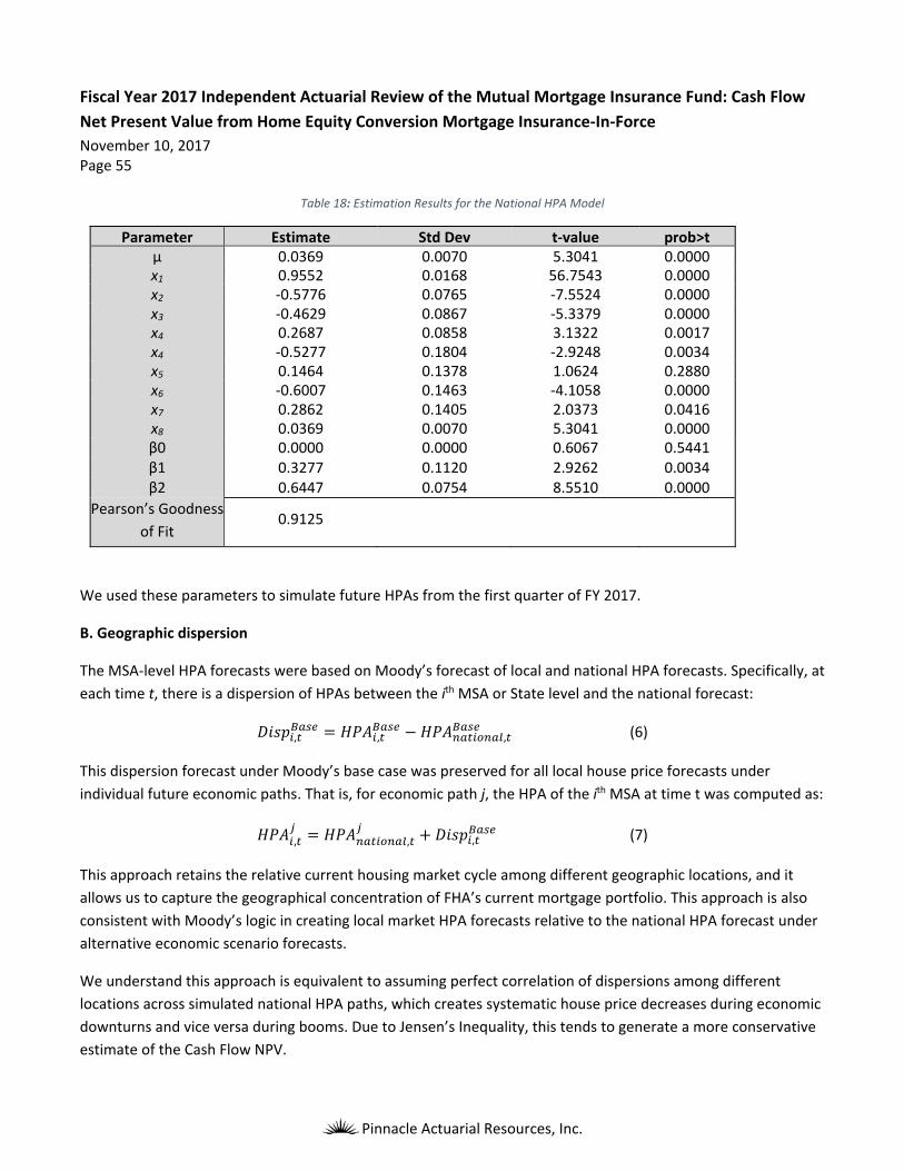
Fiscal Year 2017 Independent Actuarial Review of the Mutual Mortgage Insurance Fund: Cash Flow
Net Present Value from Home Equity Conversion Mortgage Insurance‐In‐Force November 10, 2017 Page 55
Pinnacle Actuarial Resources, Inc.
Table 18: Estimation Results for the National HPA Model
Parameter Estimate Std Dev t‐value prob>t µ 0.0369 0.0070 5.3041 0.0000 x1 0.9552 0.0168 56.7543 0.0000 x2 ‐0.5776 0.0765 ‐7.5524 0.0000 x3 ‐0.4629 0.0867 ‐5.3379 0.0000 x4 0.2687 0.0858 3.1322 0.0017 x4 ‐0.5277 0.1804 ‐2.9248 0.0034 x5 0.1464 0.1378 1.0624 0.2880 x6 ‐0.6007 0.1463 ‐4.1058 0.0000 x7 0.2862 0.1405 2.0373 0.0416 x8 0.0369 0.0070 5.3041 0.0000 β0 0.0000 0.0000 0.6067 0.5441 β1 0.3277 0.1120 2.9262 0.0034 β2 0.6447 0.0754 8.5510 0.0000
Pearson’s Goodness
of Fit 0.9125
We used these parameters to simulate future HPAs from the first quarter of FY 2017.
B. Geographic dispersion
The MSA‐level HPA forecasts were based on Moody’s forecast of local and national HPA forecasts. Specifically, at
each time t, there is a dispersion of HPAs between the ith MSA or State level and the national forecast:
, , , (6)
This dispersion forecast under Moody’s base case was preserved for all local house price forecasts under
individual future economic paths. That is, for economic path j, the HPA of the ith MSA at time t was computed as:
, , , (7)
This approach retains the relative current housing market cycle among different geographic locations, and it
allows us to capture the geographical concentration of FHA’s current mortgage portfolio. This approach is also
consistent with Moody’s logic in creating local market HPA forecasts relative to the national HPA forecast under
alternative economic scenario forecasts.
We understand this approach is equivalent to assuming perfect correlation of dispersions among different
locations across simulated national HPA paths, which creates systematic house price decreases during economic
downturns and vice versa during booms. Due to Jensen’s Inequality, this tends to generate a more conservative
estimate of the Cash Flow NPV.
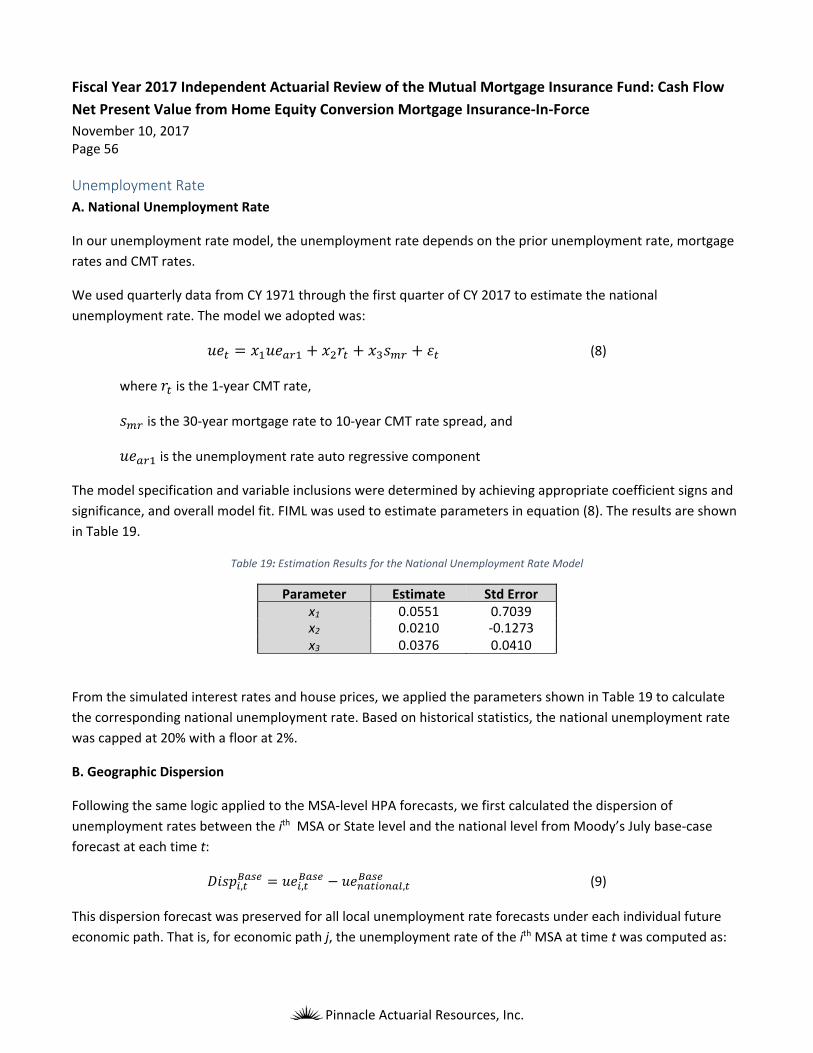
Fiscal Year 2017 Independent Actuarial Review of the Mutual Mortgage Insurance Fund: Cash Flow
Net Present Value from Home Equity Conversion Mortgage Insurance‐In‐Force November 10, 2017 Page 56
Pinnacle Actuarial Resources, Inc.
Unemployment Rate
A. National Unemployment Rate
In our unemployment rate model, the unemployment rate depends on the prior unemployment rate, mortgage
rates and CMT rates.
We used quarterly data from CY 1971 through the first quarter of CY 2017 to estimate the national
unemployment rate. The model we adopted was:
(8)
where is the 1‐year CMT rate,
is the 30‐year mortgage rate to 10‐year CMT rate spread, and
is the unemployment rate auto regressive component
The model specification and variable inclusions were determined by achieving appropriate coefficient signs and
significance, and overall model fit. FIML was used to estimate parameters in equation (8). The results are shown
in Table 19.
Table 19: Estimation Results for the National Unemployment Rate Model
Parameter Estimate Std Errorx1 0.0551 0.7039x2 0.0210 ‐0.1273x3 0.0376 0.0410
From the simulated interest rates and house prices, we applied the parameters shown in Table 19 to calculate
the corresponding national unemployment rate. Based on historical statistics, the national unemployment rate
was capped at 20% with a floor at 2%.
B. Geographic Dispersion
Following the same logic applied to the MSA‐level HPA forecasts, we first calculated the dispersion of
unemployment rates between the ith MSA or State level and the national level from Moody’s July base‐case
forecast at each time t:
, , , (9)
This dispersion forecast was preserved for all local unemployment rate forecasts under each individual future
economic path. That is, for economic path j, the unemployment rate of the ith MSA at time t was computed as:
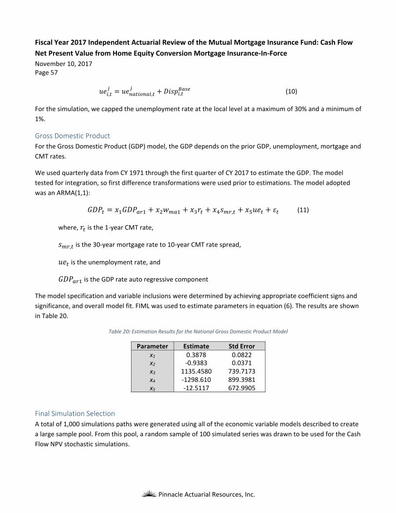
Fiscal Year 2017 Independent Actuarial Review of the Mutual Mortgage Insurance Fund: Cash Flow
Net Present Value from Home Equity Conversion Mortgage Insurance‐In‐Force November 10, 2017 Page 57
Pinnacle Actuarial Resources, Inc.
, , , (10)
For the simulation, we capped the unemployment rate at the local level at a maximum of 30% and a minimum of
1%.
Gross Domestic Product
For the Gross Domestic Product (GDP) model, the GDP depends on the prior GDP, unemployment, mortgage and
CMT rates.
We used quarterly data from CY 1971 through the first quarter of CY 2017 to estimate the GDP. The model
tested for integration, so first difference transformations were used prior to estimations. The model adopted
was an ARMA(1,1):
, (11)
where, is the 1‐year CMT rate,
, is the 30‐year mortgage rate to 10‐year CMT rate spread,
is the unemployment rate, and
is the GDP rate auto regressive component
The model specification and variable inclusions were determined by achieving appropriate coefficient signs and
significance, and overall model fit. FIML was used to estimate parameters in equation (6). The results are shown
in Table 20.
Table 20: Estimation Results for the National Gross Domestic Product Model
Parameter Estimate Std Errorx1 0.3878 0.0822x2 ‐0.9383 0.0371x3 1135.4580 739.7173x4 ‐1298.610 899.3981x5 ‐12.5117 672.9905
Final Simulation Selection
A total of 1,000 simulations paths were generated using all of the economic variable models described to create
a large sample pool. From this pool, a random sample of 100 simulated series was drawn to be used for the Cash
Flow NPV stochastic simulations.

Fiscal Year 2017 Independent Actuarial Review of the Mutual Mortgage Insurance Fund: Cash Flow
Net Present Value from Home Equity Conversion Mortgage Insurance‐In‐Force November 10, 2017 Page 58
Pinnacle Actuarial Resources, Inc.
Appendix E: HECM Cash Flow Analysis This appendix describes the calculation of the Cash Flow NPV. Future cash flow calculations are based on
forecasted variables, such as HPI and interest rates, in addition to individual mortgage characteristics and
borrower behavior assumptions. HECM cash flows are discounted according to the latest discount factors
published by the OMB.
General Approach to Mortgage Termination Projections
HECM termination rates are projected for all future policy years for each surviving (active) mortgage. The
variables used in the projection are derived from mortgage characteristics and economic forecasts. OMB
Economic Assumptions and Moody’s September 2017 forecasts of interest, unemployment rates and HPI are
combined with the mortgage‐level data to simulate the projected economic paths and create the necessary
forecasted variables. MSA‐level forecasts of HPI apply to mortgages in metropolitan areas; otherwise mortgages
use the state‐level HPI forecasts. House price forecasts are generated simultaneously with various
macroeconomic variables including the local unemployment rates.
For each mortgage during future policy years, the derived mortgage variables serve as independent variables to
the multinomial logistic termination models described in Appendix B. The termination projections by claim type
are then calculated to generate the probability of mortgage termination in a policy year by different modes of
termination given that it survives to the end of the prior policy year. The HECM cash flow model uses these
forecasted termination rates to project the cash flows associated with different termination events. Based on
the specific characteristics of the mortgage, the probability of each termination is calculated. Then, a random
number between 0 and 1 is generated, and based on this random draw a mortgage transition is determined. The
projection process continues for each mortgage until the mortgage ends by termination or claim.
Cash Flow Components
There are four major components of HECM cash flows:
1. MIP,
2. claims,
3. note holding expenses, and
4. recoveries on notes in inventory (after assignment).
Premiums consist of upfront and annual MIPs, which are inflows to the HECM program. Recoveries are the
property recovery amount received by FHA at the time of note termination after assignment, which is the
minimum of the mortgage balance and the predicted net sales proceeds at termination. The recovery amount
for refinance termination is always the mortgage balance. Claim Type 1 (CT1) payments are cash outflows paid
to the lender when the net proceeds of a property sale are insufficient to cover the balance of the mortgage.
Assignment claims and note holding payments are additional outflows. Table 21 summarizes the HECM inflows
and outflows.
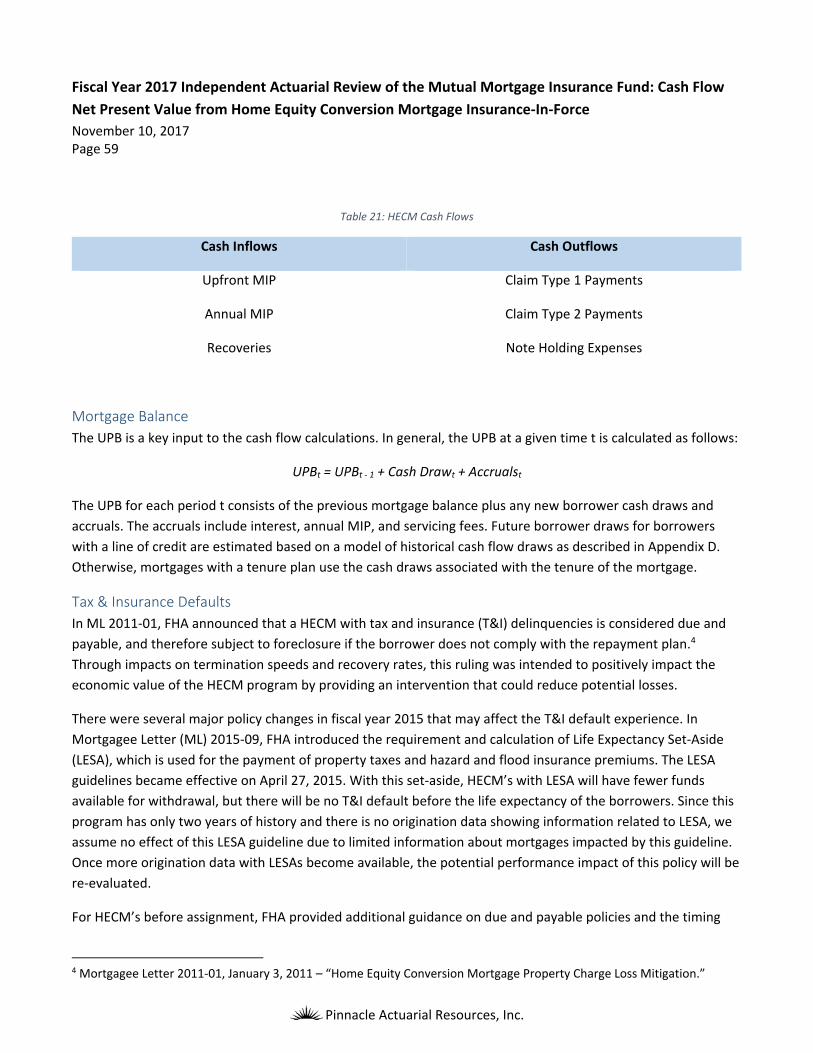
Fiscal Year 2017 Independent Actuarial Review of the Mutual Mortgage Insurance Fund: Cash Flow
Net Present Value from Home Equity Conversion Mortgage Insurance‐In‐Force November 10, 2017 Page 59
Pinnacle Actuarial Resources, Inc.
Table 21: HECM Cash Flows
Cash Inflows Cash Outflows
Upfront MIP Claim Type 1 Payments
Annual MIP Claim Type 2 Payments
Recoveries Note Holding Expenses
Mortgage Balance
The UPB is a key input to the cash flow calculations. In general, the UPB at a given time t is calculated as follows:
UPBt = UPBt ‐ 1 + Cash Drawt + Accrualst
The UPB for each period t consists of the previous mortgage balance plus any new borrower cash draws and
accruals. The accruals include interest, annual MIP, and servicing fees. Future borrower draws for borrowers
with a line of credit are estimated based on a model of historical cash flow draws as described in Appendix D.
Otherwise, mortgages with a tenure plan use the cash draws associated with the tenure of the mortgage.
Tax & Insurance Defaults
In ML 2011‐01, FHA announced that a HECM with tax and insurance (T&I) delinquencies is considered due and
payable, and therefore subject to foreclosure if the borrower does not comply with the repayment plan.4
Through impacts on termination speeds and recovery rates, this ruling was intended to positively impact the
economic value of the HECM program by providing an intervention that could reduce potential losses.
There were several major policy changes in fiscal year 2015 that may affect the T&I default experience. In
Mortgagee Letter (ML) 2015‐09, FHA introduced the requirement and calculation of Life Expectancy Set‐Aside
(LESA), which is used for the payment of property taxes and hazard and flood insurance premiums. The LESA
guidelines became effective on April 27, 2015. With this set‐aside, HECM’s with LESA will have fewer funds
available for withdrawal, but there will be no T&I default before the life expectancy of the borrowers. Since this
program has only two years of history and there is no origination data showing information related to LESA, we
assume no effect of this LESA guideline due to limited information about mortgages impacted by this guideline.
Once more origination data with LESAs become available, the potential performance impact of this policy will be
re‐evaluated.
For HECM’s before assignment, FHA provided additional guidance on due and payable policies and the timing
4 Mortgagee Letter 2011‐01, January 3, 2011 – “Home Equity Conversion Mortgage Property Charge Loss Mitigation.”

Fiscal Year 2017 Independent Actuarial Review of the Mutual Mortgage Insurance Fund: Cash Flow
Net Present Value from Home Equity Conversion Mortgage Insurance‐In‐Force November 10, 2017 Page 60
Pinnacle Actuarial Resources, Inc.
requirements in ML 2015‐105 and ML 2015‐116. For HECM’s after assignment, FHA currently does not foreclose
on assigned mortgages that are in T&I default. In order to secure and maintain FHA’s position on the lien of an
assigned mortgage, FHA advances T&I payments on behalf of the borrower. FHA first advances funds from the
borrower’s available HECM funds. If no funds are available, FHA advances the tax payment and adds the
payment amount to the UPB. These policies affect all existing books and future books.
For unassigned mortgages, if a mortgage goes to into default, the lender may provide a separate mortgage to
the borrower to cover the T&I. If this occurs, once a mortgage becomes eligible for assignment, it will not be
able to be assigned until the separate mortgage is satisfied.
For assigned mortgages, the T&I payments are treated as note holding expenses, a component of cash outflows,
and added to the UPB. The projected T&I payments are not projected separately, but are included in the
projection of note holding expenses.
MIP
Upfront and annual MIP, along with recoveries, are the sources of FHA revenue from the HECM program.
Borrowers typically finance the upfront MIP when taking out a HECM mortgage. Similarly, the recurring annual
MIP is added to the balance of the mortgage.
The upfront MIP is paid to FHA at the time of mortgage closing. It is equal to a stated percentage of the MCA.
Since fiscal year 2009, the upfront MIP rate for the Standard HECM contract has been 2% of the MCA. This rate
remained the same for the Standard program through fiscal year 2013. For 2011 through 2013 cohorts, the
upfront MIP rate for the Saver program was 0.01% of the MCA. For the new program introduced in fiscal year
2014, the upfront MIP rate is 0.5% of the MCA if the first‐year cash draw is less than or equal to 60% of the
initial PL, and 2.5% of MCA if the first‐year cash draw is more than 60% of the initial PL. Typically, the upfront
MIP is financed by the HECM lender. The upfront MIP is paid in full to FHA at the mortgage closing, and is a
positive cash flow.
The annual MIP is calculated as a percentage of the current mortgage balance. For the 2009 and 2010 cohorts,
the annual MIP is 0.5% of the UPB. From fiscal year 2011 and forward, the annual MIP is 1.25% of the UPB for all
Standard, Saver, and the new program introduced in fiscal year 2014. Before a mortgage is assigned, the annual
MIP is assumed to be advanced by the lender, paid to FHA, and added to the accruing mortgage balance.
Claims
Claims made by lenders consist of CT1 and Claim Type 2 (CT2).
CT1 enters the HECM cash flows as payments to the lender when a property is sold and the net proceeds from
the sale are not sufficient to cover the balance of the mortgage at termination. The CT1 payment for a mortgage
5 Mortgagee Letter 2015‐10, April 23, 2015 – “Home Equity Conversion Mortgage (HECM) Due and Payable Policies.” 6 Mortgagee Letter 2015‐11, April 23, 2015 – “Loss Mitigation Guidance for Home Equity Conversion Mortgages (HECMs) in Default due to Unpaid Property Charges.”

Fiscal Year 2017 Independent Actuarial Review of the Mutual Mortgage Insurance Fund: Cash Flow
Net Present Value from Home Equity Conversion Mortgage Insurance‐In‐Force November 10, 2017 Page 61
Pinnacle Actuarial Resources, Inc.
that terminates without assignment is expressed as:
Claim Type 1 Payment = maximum (0, UPB ‐ Net Property Sales Price)
The net sales price of the property is:
Net Property Sales Price = Estimated Property Sales Price × (1 – sales expenses % – other expenses %)
The estimated property sale price is calculated using formulaically derived HPA values and empirically estimated
Maintenance Risk Adjustment (MRA) factors. The MRA factors vary by period number and are determined such
that the expected CT1 claim severity rate after applying the MRA to the projected home appraisal value is equal
to the observed CT1 claim severity rate.
Sales expenses are those required to conduct the actual sale, and other expenses are those incurred to manage
the property until the sale.
Sales and other expenses are estimated to be 25% of the sales price based on home sale data provided by FHA.
This is based on data related to the sale of over 6,000 FHA owned properties.
Lenders can assign a mortgage to FHA when the UPB reaches 98% of the MCA. A CT2 occurs when FHA acquires
the note resulting in a cash outflow, the acquisition cost, which is the mortgage balance (up to the MCA). The
ultimate net losses from CT2 depends on two components: the note holding expenses after assignment and
recoveries from assigned notes.
FHA imposes a set of requirements that, if any of them are not met, makes the HECM ineligible for assignment
even when UPB reaches 98% of the MCA. We project the probability of assignment based on historical data by
the number of quarters the mortgage has been eligible for assignment as follows:
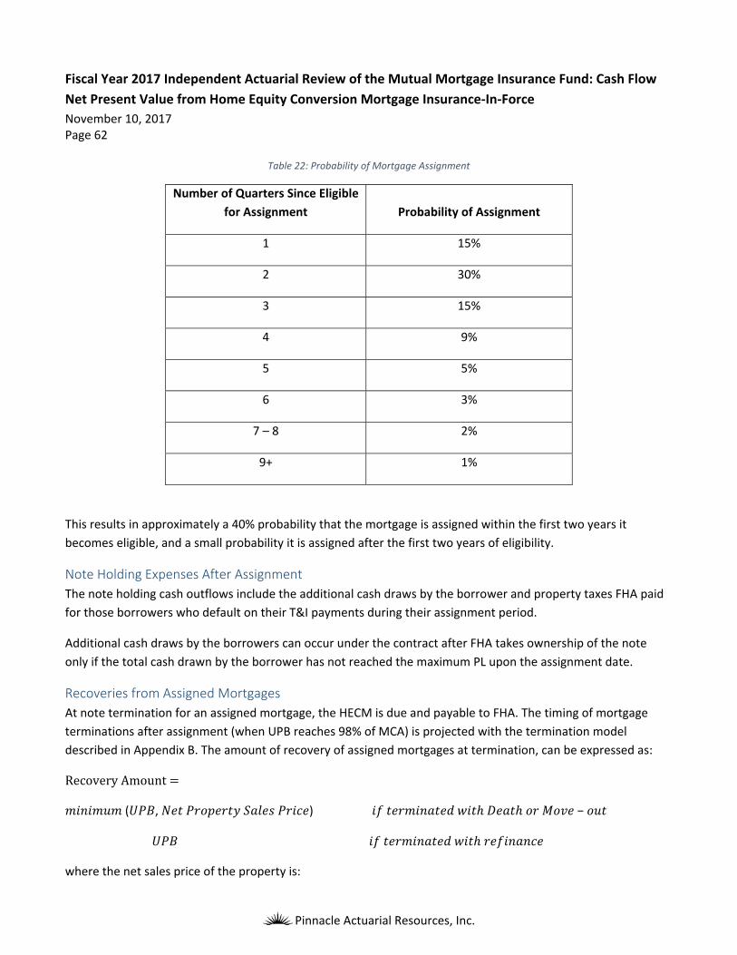
Fiscal Year 2017 Independent Actuarial Review of the Mutual Mortgage Insurance Fund: Cash Flow
Net Present Value from Home Equity Conversion Mortgage Insurance‐In‐Force November 10, 2017 Page 62
Pinnacle Actuarial Resources, Inc.
Table 22: Probability of Mortgage Assignment
Number of Quarters Since Eligible
for Assignment
Probability of Assignment
1 15%
2 30%
3 15%
4 9%
5 5%
6 3%
7 – 8 2%
9+ 1%
This results in approximately a 40% probability that the mortgage is assigned within the first two years it
becomes eligible, and a small probability it is assigned after the first two years of eligibility.
Note Holding Expenses After Assignment
The note holding cash outflows include the additional cash draws by the borrower and property taxes FHA paid
for those borrowers who default on their T&I payments during their assignment period.
Additional cash draws by the borrowers can occur under the contract after FHA takes ownership of the note
only if the total cash drawn by the borrower has not reached the maximum PL upon the assignment date.
Recoveries from Assigned Mortgages
At note termination for an assigned mortgage, the HECM is due and payable to FHA. The timing of mortgage
terminations after assignment (when UPB reaches 98% of MCA) is projected with the termination model
described in Appendix B. The amount of recovery of assigned mortgages at termination, can be expressed as:
RecoveryAmount
( , ) −
where the net sales price of the property is:

Fiscal Year 2017 Independent Actuarial Review of the Mutual Mortgage Insurance Fund: Cash Flow
Net Present Value from Home Equity Conversion Mortgage Insurance‐In‐Force November 10, 2017 Page 63
Pinnacle Actuarial Resources, Inc.
Net Property Sales Price = Estimated Property Sales Price × (1 – sales expenses % – other expenses %)
Sales expenses are those required to conduct the actual sale, and other expenses are those to manage the
property until the sale. Sales expenses plus other expenses are estimated to be 25% based on historical HECM
data.
Net Future Cash Flows
The Cash Flow NPV for the HECM book of business is computed by summing the individual components as they
occur over time:
Net Cash Flowt = Annual Premiumst + Recoveriest ‐ Claim Type 1t ‐ Claim Type 2t ‐ Note Holding Expensest
Discount Factors
The discount factors applied were provided by FHA and reflect the most recent Treasury yield curve, which
captures the Federal government’s cost of capital in raising funds. These factors reflect the capital market’s
expectation of the consolidated interest risk of U.S. Treasury securities. Our simulations aggregated each future
year’s cash flows, which are treated as being received at the end of the year.