Embed Size (px)
Citation preview

CEP Discussion Paper No 762
December 2006
An R&D-Based Model of Multi-Sector Growth
L. Rachel Ngai and Roberto M. Samaniego

Abstract We develop a multi-sector general equilibrium model in which productivity growth is driven by the production of sector-specific knowledge. In the model, we find that long run differences in total factor productivity growth across sectors are independent of the parameters of the knowledge production function except for one, which we term the fertility of knowledge. Differences in R&D intensity are also independent of most other parameters. The fertility of knowledge in the capital sector is central to the growth properties of the model economy. JEL Codes: D24, D92, O31, O41, Keywords: Endogenous technical change, multisector growth, fertility of knowledge, total factor productivity, R&D intensity, investment-specific technical change. Pigmaei gigantum humeris impositi plusquam ipsi gigantes vident. — Bernard of Chartres, circa 1100. This paper was produced as part of the Centre’s Macro Programme. The Centre for Economic Performance is financed by the Economic and Social Research Council. Acknowledgements The authors are grateful to Anna Ilyina, Chris Pissarides, Mark Schankerman, Tara Sinclair, and participants at the George Washington University Macro-International Seminar for helpful discussions and suggestions. Comments welcome. All errors and omissions are the authors’. L. Rachel Ngai is an Associate of the Macro Programme at the Centre for Economic Performance and a Lecturer in the Department of Economics, London School of Economics, (email: [email protected]). Roberto M. Samaniego is an Assistant Professor in the Department of Economics, The George Washington University, Washington, DC, USA (email: [email protected]). Published by Centre for Economic Performance London School of Economics and Political Science Houghton Street London WC2A 2AE All rights reserved. No part of this publication may be reproduced, stored in a retrieval system or transmitted in any form or by any means without the prior permission in writing of the publisher nor be issued to the public or circulated in any form other than that in which it is published. Requests for permission to reproduce any article or part of the Working Paper should be sent to the editor at the above address. © L. R. Ngai and R. M. Samaniego, submitted 2006 ISBN 0 7530 2068 8
1 Introduction
Total factor productivity (TFP) growth rates vary widely and persistently acrossindustries.1 However, economic growth rates for aggregate variables are known to befairly constant in the long run. What industry-level parameters might lie behind theobserved differences in TFP growth rates? How can one reconcile the observation ofa stable aggregate growth path with diverging productivity at the industry level?This paper answers these questions using a general equilibrium model of endoge-
nous productivity change. In the model, TFP growth is the outcome of researchactivity, which produces economically useful knowledge. Industries differ in terms ofa number of factors that affect the returns to R&D activity, including the determi-nants of the demand for their goods, and the parameters of the production functionfor new knowledge. We investigate which of these factors lead to cross-industry dif-ferences in TFP growth rates and R&D intensity, and study under what conditionsthe economy possesses an aggregate balanced growth path (BGP).Our framework is a multi-sector growth model and contains a number of factors
that have been thought to affect the returns to R&D.2 In addition, we consider onenew potential source of cross-industry variation: the extent to which old knowledge isuseful for the production of new knowledge. We call this the fertility of knowledge.In a class of one-sector growth models, Jones (1995) shows that the value of thisparameter must be less than unity if the aggregate economy is to possess a balancedgrowth path that is consistent with the data. Otherwise, the economy displays "scaleeffects": larger countries grow faster, and countries with growing populations woulddisplay accelerating growth.3
Allowing for R&D in a multi-sector framework, we find that a BGP requiresrestrictions only on the fertility parameter of the industries that produce capitalgoods. Allowing capital to be an input in the production of knowledge, this restrictionis that "average" fertility in these sectors must be bounded from above by a numberstrictly less than one. The upper bound is a function of the capital share of costs.Strikingly, we find that the equilibrium ranking of TFP growth rates across sectors
depends only on cross-industry differences in the fertility of knowledge. While theresult is stark, the role of the fertility parameter in a one-sector context provides some
1For example, among capital goods, Jorgenson et al (2005) estimate that annual TFP growthrates in the United States over the period 1960-2004 range from -1.0% per year in Structures to10.4% in Computers and Office Equipment.
2A small sample of the related literature includes Romer (1990), Aghion and Howitt (1992) andJones (1995) on R&D-based models of economic growth, and Pakes and Schankerman (1984), Jaffe(1986) and Cohen and Levin (1989) on R&D intensity.
3In the terminology of Jones (2005a), these are "strong" scale effects.
2

intuition. In a one-sector model, eliminating aggregate scale effects by introducingdecreasing returns to knowledge also eliminates the effects of other parameters andpolicy variables on equilibrium rates of economic growth. In a multi-sector context,a similar result applies to the parameters that determine the returns to R&D. Theseparameters may affect sectoral differences in R&D intensity, and even the size of eachsector, but only the fertility of knowledge affects the rate at which inputs accumulaterelative to each other — including knowledge.4 The key to this result, however, is notthat fertility is limited in each sector, but that TFP growth in each sector must bestable over time.Our results address some fundamental issues regarding the nature of aggregate
growth and in particular growth accounting exercises. A notable feature of post-war US data is a secular decline in relative price of capital, and this phenomenon iswidely attributed investment-specific technical change: productivity improvementsthat affect primarily the capital goods sector. Greenwood et al (1997) and Cumminsand Violante (2002) ascribe approximately 60% of economic growth to investment-specific technical change and suggest that this is a significant channel for postwarUS economic growth. Investment-specific technical change in our model can ariseendogenously when the fertility of knowledge is higher in the durable goods sector.In a calibrated version of the model, we find that the model economy is broadly
consistent with the distribution of income and employment across activities, and withthe ranking of TFP growth rates across types of capital. The fertility of knowledgevaries widely across sectors, but we find fertility values to be typically quite low,except in the fastest-growing sectors.In related work, Klenow (1996) studies the determinants of cross-sectoral TFP
growth differences in a version of Romer’s (1990) model, in which R&D results ina growing number of intermediates. However, that model has scale effects at theindustry level, and this is what largely drives the theoretical results. Acemoglu andGuerrieri (2006) develop a two-sector endogenous growth model in which growth isdriven by the production of knowledge. Their model does not identify the techno-logical determinants of R&D intensity across industries but focuses instead on therole of different capital shares across industries. In Krusell (1998), R&D leads toinvestment-specific technical change, as it can do here. However, R&D only oc-curs in the capital goods sector, so it is unsuitable for cross-industry comparisons.Vourvachaki (2006) also develops an endogenous growth model with two final goodsectors, but again R&D only occurs in one sector.Section 2 describes the structure of the model, and Section 3 studies analytically
4This is consistent with the observation that R&D intensity varies much more in cross sectionsthan do TFP growth rates. See Klenow (1996) and Burnside (1996).
3

its long run behavior. Section 4 explores the quantitative implications of our results.Section 5 provides with more discussion on the knowledge production function. Sec-tion 6 concludes.
2 Economic Environment
The economy consists of z sectors, where firms in sectors i ∈ {1, ..m− 1} produceconsumption goods, whereas firms in sectors j ∈ {m, ...z} produce investment goods.Each good comes in a continuum of differentiated varieties, and is produced usingcapital and labor as physical inputs. The productivity of a firm in any given sectordepends upon the quantity of technical knowledge or "ideas" at its disposal. Newknowledge is produced as a result of individual firm activity, and spillovers fromother firms.
2.1 Households
Time is discrete and indexed by t. There is a continuum of households of measureNt = gtN . Households have preferences over a finite number of different goods i ∈{1, ..m− 1}, each of which comes in a continuum of varieties h ∈ [0, 1]. The life-timeutility of a household is
∞Xt=0
(βgN)t c1−θt − 11− θ
(1)
ct =m−1Qi=1
µcitωi
¶ωi
, cit =µZ 1
0
cμi−1μi
iht dh
¶ μiμi−1
i = 1, ..m− 1 (2)
where β is the discount factor, βgN < 1, θ > 0, μi > 1, ωi > 0 andP
i ωi = 1.The parameter μi is the elasticity of substitution across different varieties of goodi, and 1/θ is the intertemporal elasticity of substitution. The life-time utility is alogarithmic function of ct when θ = 1.We use lower case letters to denote per-capitavariables. In most of what follows, i indexes a consumption sector or good, j indexesa type of capital, and h indexes a firm in any given sector.Each household member is endowed with one unit of labor and kt units of capital.
They earn income by renting capital and labor to firms, and by earning profits fromthe firms. Their budget constraint is
m−1Xi=1
Zpihtcihtdh+
zXj=m
Zpjhtxjhtdh ≤ wt +Rtkt + πt (3)
4

where xjht is investment in variety h of capital good j, piht is the price of variety h
of good i, wt and Rt are rental prices of labor and capital, and Ntπt ≡zP
i=1
R 10Πihtdh
equals total profits from firms.The capital accumulation equation is gNkt+1 = xt + (1− δk) kt The composite
investment good xt is produced via a Cobb-Douglas function of all capital types j, sothe elasticity of substitution across capital goods j is equal to one, while the elasticityof substitution across different varieties of capital good j is equal to μj > 1 :
xt =Qz
j=m
µxjtκj
¶κj
, xjt =∙Z
x(μj−1)/μjjht dh
¸μj/(μj−1)j = m, ..z (4)
where κj > 0 andP
j κj = 1. We define the price index for the consumptioncomposite ct and the investment composite respectively as:
pct ≡Pm−1
i=1
R 10pihtcihtdh
ct; pxt ≡
Pzj=m
R 10pjhtxjhtdh
xt. (5)
2.2 Firms
The production function for variety h of good i is
Yiht = TihtKαihtN
1−αiht (6)
where α ∈ (0, 1), Tiht is knowledge, Yiht is output, Kiht is capital and Niht is labor.Let Fiht be knowledge produced by firm h in sector i ≤ h. Knowledge accumulates
over time according to the function
Tih,t+1 = Fiht + (1− δT )Tiht (7)
where new knowledge is produced according to the function
Fiht = Ai
¡T 1−σiiht T σi
it
¢φi QαihtL
1−αiht (8)
where Qiht and Liht are capital and labor used in production of knowledge, andTit =
R 10Tihtdh. The knowledge production function has constant returns to rival-
rous inputs (capital and labor). In this case, following the empirical literature, theequilibrium stock of knowledge equals the depreciated stock of R&D spending. Westudy the implications of diminishing returns (or duplication in research) in Section(5).5
5The capital share is the same as in the final goods production function. This allows us toderive closed-form solutions: more importantly, it implies that the production function differsacross sectors only in terms of the TFP index Tih, which is the focus of the paper.
5

The literature has focused on several factors that may determine cross-industryR&D intensity differences. A survey by Cohen and Levin (1989) identifies thembroadly as: market size, technological opportunity, and spillovers. In our model,industries may differ in terms of five parameters: μi, ωi, Ai, σi and φi. The first two,μi and ωi, are preference parameters, that determine the scope and sensitivity of po-tential returns to R&D. The remaining parameters are technological, and determinethe structure of the knowledge production function. Pakes and Schankerman (1984)identify technological opportunity as a constant in the ideas’ production function,similar to our parameter Ai. Our formulation of knowledge spillovers σi is as inKrusell (1998).In the model, knowledge is a persistent stock which may be increased by research.
The amount of new knowledge generated by research is a function of the quantityof inputs used, and the quantity of pre-existing knowledge. Parameter σi ∈ [0, 1)indicates the extent to which firms in sector i benefit from the knowledge of theircompetitors.6 We denote γiht ≡ Tiht+1/Tiht as the growth factor of Tih. Parameterφi ∈ R captures the extent to which pre-existing knowledge is useful for the produc-tion of new knowledge. We will be say that if φi > φi0 then sector i is more fertilethan sector i0.In a one-sector context, our notion of "fertility" is referred to as the "intertem-
poral knowledge spillover," or the "measure of decreasing returns to ideas." Its effecton the knowledge stock when positive is referred to as "standing on shoulders," andwhen negative as "fishing out." In the former case, knowledge becomes easier toproduce as it accumulates, whereas in the latter case it becomes more difficult. Oneof our innovations is to present fertility as a potential source of cross-industry vari-ation and, as a result, we feel it is appropriate to introduce new and more conciseterminology.Each sector i ≤ z is monopolistically competitive. Taking its demand function as
given, a firm h in sector i chooses optimally its level of production and R&D inputsin order to maximize the discounted stream of real profits,
∞Pt=0
λtΠiht
pct(9)
where λt is the discount factor at time t, with λ0 = 1, and λt =tQ
s=1
11+rt
for t ≥ 1,
6In the model there are no cross-sectoral spillovers. We study such spillovers in Section (5) .Empirical research finds mostly weak spillovers across firms within narrow, related sectors, but doesnot find measurable spillovers across broad sectors — see Bernstein and Nadiri (1988) and (1989)and Schultz (2006).
6

where rt is the real interest rate. The firm’s profits are given by
Πiht = pihtYiht − wt (Niht + Liht)−Rt (Kiht +Qiht) (10)
3 Decentralized Equilibrium
Definition 1 A decentralized equilibrium consists of sequences of prices and of al-locations such that:
1. Given the sequence of pricesnn(piht)h∈[0,1]
ozi=1
, Rt, wt
ot=0,1..
, households choosenn(ciht, xiht)h∈[0,1]
ozi=1
ot=0,1,...
to maximize their discounted stream of utility
(1);
2. Given the sequence of input prices {Rt, wt}t=0,1.. , and taking their demand func-tions as given, firms choose
nn(Kiht, Niht, Qiht, Liht)h∈[0,1]
ozi=1
ot=0,1...
to maxi-
mize discounted stream of profit (9);
3. The sequence of input prices {Rt, wt}t=0,.. satisfies the capital and labor marketclearing conditions in all periods:
zPi=1
Z 1
0
(Kiht +Qiht) = Kt,zP
i=1
Z 1
0
(Niht + Liht) = Nt (11)
Our objective is to understand dynamics across broad sectors of the economyand not across different varieties of any given good. Therefore, we focus on sym-metric equilibria across varieties within each sector i and suppress the firm index hhenceforth.The equilibrium results are summarized in the following claims. All proofs are
given in the Appendix.
Lemma 1 In equilibrium,
Kit
Nit=
Qjt
Ljt∀i, j, and pit
pjt=
Tjt¡1− 1/μj
¢Tit (1− 1/μi)
. (12)
The intuition is that competitive input markets require marginal rates of technicalsubstitution across labor and capital to be equalized across firms. The assumptionof the Cobb-Douglas production function with equal capital shares across activities
7

then delivers the results. Under (12), the capital market-clearing condition thenimplies that the aggregate capital-labor ratio k is also the capital-labor ratio forboth production and R&D activities. This facilitates the proof of the followingaggregation result.
Lemma 2 Let 1/μx =Pz
i=m κi (1/μi). The investment sectors j ∈ {m, ..., z} can beaggregated into one sector with a production function
Ntxt ≡ Txt³Pz
j=mKjt
´α ³Pzj=mNjt
´1−α(13)
where the knowledge index Txt equals
Txt =
"zQ
j=m
µ1− 1/μj1− 1/μx
¶#zQ
j=m
Tκjjt (14)
The result derives the production function for the investment composite xt fromthe optimal input allocations for sectors j ∈ {m, ..., z} . It also shows that the markupfor the composite investment good is a weighted average of the markups in eachinvestment sector. We denote γxt = Tx,t+1/Txt :
γxt =zQ
j=m
γκjjt . (15)
Lemma 2 is an aggregation result which allows us to relate the rental price of capitalto the TFP index of composite investment goods, which simplifies the Euler conditionfor the consumer in the following Lemma. Let qt be the relative price of capital andGt the gross return on investment in terms of capital goods. Then,
qt =pxtpct
Gt ≡ 1− δk +Rt
pxt. (16)
Lemma 3 The Euler condition for the consumer satisfies
1
β
µct+1ct
¶θ
=qt+1qt
Gt+1 (17)
where the equilibrium physical gross return of investment is:
Gt = 1− δk + αTxtkα−1t
µ1− 1
μx
¶. (18)
8

The key of the proof is to derive Rt/pxt as function of Txt and pxt/pjt follows(12). We next turn to the dynamic decisions for the firm. Define ni ≡ Ni/N andli ≡ Li/N as the employment shares for production and R&D activities in sector i.
Lemma 4 The firm’s dynamic optimization implies
Gt+1γφiit
γxt= Aik
αt+1Nit+1T
φi−1it+1 + φi (1− σi)
¡γit+1 − 1 + δT
¢+ 1− δT , ∀i (19)
Equation (19) is derived from the optimal Tiht+1 chosen by the firm. If χiht is theshadow price for knowledge Tiht+1, then
χiht =
∙λt+1piht+1pct+1
∂Yiht+1∂Tiht+1
¸future production
+
∙χiht+1
∂Fiht+1
∂Tiht+1
¸future research
+£χiht+1 (1− δT )
¤future knowledge
(20)
The equation reflect three benefits of the production of more knowledge: (1) moreefficient production of goods and services at time t+ 1, (2) more efficient productionof knowledge at time t+ 1, and (3) more future knowledge. The equilibrium χiht isdetermined by equating the marginal benefit and marginal cost of research efforts(Qiht and Liht), e.g. for Liht
χiht∂Fiht
∂Liht=
λtpct
∂Πiht+1
∂Liht(21)
The key to equation (19) is that some of these terms depend on the rate atwhich technology improves — due to changes in the relative prices of final goods andchanges in shadow price of knowledge, whereas others depend on its level — due to thecurrent cost of resources. Rational researchers must thus make a trade-off betweenboth dynamic and static concerns. If the economy displays a balanced growth path,the dynamic elements of this decision problem must be constant. For the terms thatare expressed in levels to also be constant, however, requires the growth rates of theircomponent variables to offset each other. In the case of equation (19), this suggeststhat, the long run growth rate of TFP might be related to the (endogenous) growthrate of the capital stock, to the growth rate of the population, and to coefficientsthat affect the balance between these growth rates — in this case α and fertility φi.
3.1 Aggregate Balanced growth path
We look for a balanced growth path (BGP) where aggregate variables are growing atthe same constant rate but sectoral TFP growth rates are different.7 More precisely,
7Note that if γi are the same across sectors, then Lemma 1 implies that relative prices areconstant, then the model essentially reduces to a one-sector growth model.
9

such a BGP requires a constant consumption-capital ratio which in our model isthe expression c/ (qk). As in a one-sector model, certain conditions are required forsolutions to be interior solutions, and for transversality conditions to be satisfied. Wedistinguish between these two sets of conditions for balanced growth in a multi-sectormodel by stating them in separate Propositions.Define φx and φc such that
1
1− φx=
zPj=m
κj1− φj
;1
1− φc=
m−1Pi=1
ωi
1− φi(22)
and define Φ and Υ as:
Φ ≡µ1− φx −
α
1− α
¶−1; Υ =
1− φx1− φc
+α
1− α(23)
Proposition 1 Suppose there exists an equilibrium with li, ni > 0 that satisfy thetransversality conditions for Ti and k. If
Φ,Υ > 0 (24)
then there exists a unique aggregate balanced growth path. Along this path c/q and kgrow by a constant factor (γ∗x)
1/(1−α), and c grows by a constant factor (γ∗x)Υ , where
γ∗x = gΦN . (25)
Finally, knowledge Ti grows by a factor γ∗i where
(γ∗i )1−φi = (γ∗x)
1−φx ∀i. (26)
Proposition 2 Along the balanced growth path, li, ni > 0, and the transversalityconditions for Ti and k are satisfied if
β < (1/gN)1+(1−θ)ΦΥ , and (27)
∀i, φi (1− σi) < 1, gΦ/(1−φi)N ≥ (1− δT )
1/(1−φx)
Corollary 1 A BGP exists with R&D in all sectors provided conditions (24) and(27) are satisfied.
The key of the proof is to observe from (18) that k grows by a factor γ1/(1−α)x ,which by (15) is constant if γi is constant in all the capital sectors. We then use theoptimal R&D condition (19) to derive the condition for constant values of γj. The
10

upped bound on β is required for the transversality conditions. Then (19) impliesφi (1− σi) < 1 is sufficient for positive ni. Finally, the knowledge accumulationequation (7) implies that li is positive if future knowledge exceeds the stock of existingknowledge after depreciation, i.e. γi ≥ 1 − δT , then (26) implies that g
1/(1−φi)N ≥
(1− δT )1/(1−φx) is required for positive li. It is worth noting that positive li, and in
general the existence of an aggregate balanced growth path, does not imply positiveTFP growth when δT > 0.A comparison of our main result with Jones (1995) is useful. Jones (1995) presents
a one-sector model, in which the growth equation (25) holds but with Φ = λ/(1 −φ),where λ is a positive constant and φ is the one-sector model fertility parameter. Sohis condition for existence of a BGP is φ < 1. In our model balanced growth restrictsonly the weighted average of fertility parameters across capital goods: φx < 1 isnecessary for Φ > 0 (although not sufficient). No such restrictions are requiredon the fertility parameters in consumption goods sectors, or on the average for thewhole economy, since φc < 1 is not necessary for Υ > 0. Also, fertility need not beequal across individual sectors or bounded by unity in each and every sector. Theseresults can reconcile the theoretical predictions with estimates of aggregate fertilityparameters, such as those by Porter and Stern (2005) and Abdih and Joutz (2006),who find aggregate parameters larger than unity.Another difference between our results and Jones’s is due to the inclusion of
capital in our production function for knowledge. If α > 0 the fertility parameter φxis bounded below unity by a number that depends on the capital share. The key isthat new ideas increase the productivity of the sector that produces capital — whichis itself an input into the production of ideas — so decreasing returns to ideas aloneis not sufficient for the economy to have a BGP.Thus, we find in general that the restrictions on the fertility parameters imposed
by balanced growth depend on whether there are several sectors independently con-ducting research, on whether there is any exogenous depreciation of knowledge, onwhether there are knowledge spillovers, and on whether capital is used in the pro-duction of knowledge. When all these are absent our restrictions converge to Jones’srestriction.
3.2 Properties along the Balanced growth path
We now discuss other properties along the BGP. We first show that it satisfies theKaldor (1961) stylized facts. We then discuss the implications of the model forsectoral TFP growth and for sectoral R&D intensity under balanced growth.
11

1950 1960 1970 1980 1990 200010
15
20
2530
Year
Rea
l GD
P p
er h
ead
1950 1960 1970 1980 1990 200010
15
20
25
30
Year
Inve
stm
ent,
% o
f GD
P
1950 1960 1970 1980 1990 20000
0.5
1
Year
Rel
ativ
e pr
ice
of C
apita
l
Figure 1: US Real GDP per person (constant 2000 dollars, log scale), investment-ouput ratio, and the quality-adjusted relative price of capital in the United States,1953-2000. Sources: United States Bureau of Economic Analysis, and Cummins andViolante (2002). Real GDP per head is plotted against an exponential time trend.
12

Define y as total output per capita in consumption units:
y ≡zP
i=1
piTikαni
pc(28)
Proposition 3 Along the BGP, the consumption-output ratio, R&D expenditureshares and the real interest rate are constants.
Proposition 4 Along the BGP, sectoral TFP growth rates satisfy
γ1−φii = γ
1−φjj ∀i (29)
Thus, for any two sectors i, j with γi, γj ≥ 1, we have γi ≥ γj if and only if φi ≥ φj.
Condition (29) follows immediately from (26). It implies that along the aggregatebalanced growth path TFP growth rates can be different across sectors but they mustbe "balanced" according to their fertility. Moreover, for any two sectors with positiveTFP growth, the more fertile sector grows faster. Note that (26) implies that sectori has positive TFP growth along the aggregate balanced growth path only when itsfertility is less than unity.
Corollary 2 Along the BGP, the relative price of capital grows by a constant factor:
gq =qt+1qt
= (γ∗x)(1−φx)/(1−φc)−1 . (30)
Corollary (2) follows from Lemma 1 and Proposition 4. In the model, the rela-tive price of capital is falling as in Figure 1 when TFP growth in the "aggregate"consumption sector is slower than TFP growth in the "aggregate" capital sector. Ifproductivity growth is positive in both, then the relative price of capital is falling ifand only if φx > φc: it must be easier to build on previous knowledge in the durablegoods sector than in non-durables.Along the balanced growth path, the R&D expenditure share is the same as
R&D employment share within any sector i. Thus, we refer to li/ (li + ni) as "R&Dintensity" in any sector i.
Proposition 5 Along the balanced growth path,
nili=
Gγφii /γx − (1− δT )
γi − (1− δT )− φi (1− σi) ∀i. (31)
Thus, for any two sectors i, j with γi, γj ≥ 1, if φi ≥ φj and φi (1− σi) ≥ φj (1− σj)then li/ (li + ni) ≥ lj/ (lj + nj) .
13

Proposition 4 implies that the ranking of sectoral growth rates depends on onlyone parameter — fertility — and Proposition 5 implies that the ranking of sectoralR&D intensities depends on only two parameters — fertility and spillovers. Spilloversmatter because, to the individual firm, the private fertility of knowledge (i.e. theintertemporal spillover they perceive) is (1− σi)φi, which decreases with σi.8 Con-sequently, TFP growth rates and R&D intensity need not be correlated in the model.On the other hand, if the values of σi do not vary much across industries, then R&Dintensity and TFP growth may be correlated in the model — because both are relatedto the underlying parameter φi, not because R&D intensity causes TFP growth.Some empirical studies do find thatother factors may be related to R&D intensity,
although results can vary from paper to paper. Considering the relationship betweentheir findings and ours suggests further directions for exploration.First, Cohen and Levin (1989) provide an extensive survey of the literature on
the determinants of R&D intensity. A point that stands out from their survey andfrom the literature overall is the difficulty of identifying both adequate measuresof knowledge and adequate indicators of its correlates. For example, patent counts(sometimes weighted by citations) are a commonplace measure of knowledge output.The survey of Griliches (1990) contains a number of caveats regarding the use ofpatent data for such purposes, particularly that a central determinant of the be-havior of patent and citation-weighted patent series may lie in the institutions thatregulate the patenting process itself. Caballero and Jaffe (1993) find a decline in thefertility of research in a one-sector model, but also note that this finding is related toan increasing propensity to cite. Samaniego (in press) provides an example of howthe use of patent data may bias results if there is a systematic shift in the propensityto patent (or cite), as this would cause a divergence between the true stock of knowl-edge and its proxy. More generally, an incorrect empirical model of knowledge willlead to biased estimates of its relationship to and influence upon economic factors(including its own production function). Our approach contrasts with that of therelated literature because it does not require a measure of the knowledge stock, butrather identifies the properties of the production function for knowledge on the basisof its long run growth implications, within the model framework.Second, the related empirical work mostly lacks a notion of φi.
9 If φi is hardto identify separately from other candidate determinants of R&D or if it is corre-lated with them, then its omission may introduce biased estimates. For example,
8Proposition 5 implies a negative relationship between intra-industry spillovers and R&D inten-sity controlling for other variables (the φ0is). This is consistent with the findings of Bernstein andNadiri (1989).
9Exceptions include Caballero and Jaffe (1993) and Kortum (1997).
14

Pakes and Schankerman (1984) are unable to separately identify opportunity andappropriability in their model, but ascribe a large role in R&D intensity differencesto their combination, as reflected in an industry fixed effect. However, if the em-pirical counterpart of φi is not independently identified, it may also enter the fixedeffect. Alternatively, it could be that the determinants of φi are the same determi-nants of the other parameters — for example, if φi is related to the size or densityof the network of researchers in a given field, it could be correlated with measuresof market size, without there being any direct link between market size and R&Dintensity through demand side channels. It would be interesting to estimate R&Dintensity with a more complete set of industry variables, including a measure of φi.As noted, Caballero and Jaffe (1993) do estimate an aggregate equivalent of φi ina structural framework, but they do not report cross-industry estimates nor explorethe implications of their findings for R&D intensity.
4 Quantitative Analysis
We now turn to the quantitative implications of our model for TFP growth rates andR&D intensities. First, we would like to see whether a BGP exists for parametriza-tions that are consistent with the data. Second, given the link between TFP growthrates and fertility in the model, we would like to see what values of φi the modelsuggests are consistent with the data. Finally, the model implies that differences inR&D intensity depend only on fertility φi and spillovers σi, and it is of interest tosee which of the two might be the quantitatively dominant factor.Along the balanced growth path, TFP growth rates in the model depend on
parameters α, gN and φi, while R&D intensities depend, in addition, on δT and σi.We calibrate these parameters to post-war US data.10. First, we consider a specialcase where the economy has only one capital sector, denoted x, and one consumptionsector, denoted c. Thus, z = m = 2. As discussed in the introduction, a largeliterature studies investment-specific technical change, so the behavior of the modeleconomy in this case may shed light on the phenomenon. Second, we consider aversion in which there are many capital goods sectors, so that z > m = 2.
10Wherever possible, we use data for the period 1947-2000, as this is the time period over whichCummins and Violante (2002) report the data that we will use to impute cross-sectoral differencesin TFP growth as described below.
15
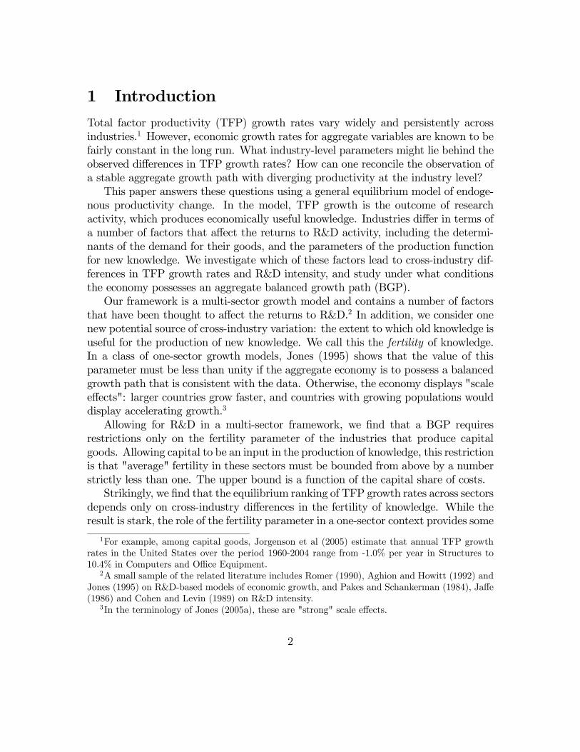
4.1 On TFP growth rates
For the 2-sector economy, Lemma 1 relates the changes in relative prices to changes inTFP growth rates, Proposition 1 links TFP growth in the capital sector to aggregategrowth, and Proposition 4 links TFP growth in the capital sector to the consumptionsector.To begin, we set α = 0.35. Values between 0.3 and 0.4 are common, so we adopt
an intermediate value. The US NIPA indicate that gy = 1.022 in consumption units,and the US Census Bureau that gN = 1.012. In the model, gy also represents thegrowth of real consumption, so gy = γ
1/(1−α)x gq where gq = γc/γx is growth in the
relative price of capital. The value of gq will be important for our quantitative results.As a benchmark, we use the quality-adjusted relative prices reported by Cumminsand Violante (2002), and explore other values below. They find that gq = 1.026−1,so that γx = 1.0313 and γc = 1.0052. These values are all that are required to deriveimplicit fertility values in the model economy.Equations (25) and (26) imply that φx = 0.075, and φc = −4.53. Thus, knowledge
in the capital goods sector weakly enhances the ability to produce new knowledge,whereas in the consumption goods sector the production of new knowledge becomesmore difficult to produce as it accumulates.To assess the sensitivity of the results to our choice of relative prices, we performed
two experiments. First, we repeated the procedure, this time using the official relativeprice of capital as reported by the Bureau of Economic Analysis. This price decreasesby 0.8% on average over the period in question, which implies a smaller divergenceof TFP across sectors. The calibrated value of γx is correspondingly lower, as is thevalue of φx. Second, we examined a range of values of gq both larger and smallerthan those suggested by the data, to see how robust the basic growth parametersof the model are to these values. Relative prices ranged between 1 — so that therelative price of capital is constant — and 1.04, above which the implied φc is toohigh for nc/lc in (31) to be positive.11 Results are reported in Table (1). Whenthe official price deflators are used instead of quality-adjusted prices, the value ofφx drops and becomes negative, although it remains close to zero. φc is larger thanbefore, since productivity growth in that sector is not as low. On the other hand,when the relative price of capital decreases by about 4% annually, TFP growth innon-durables almost shuts down, so φc become more negative. φx is positive, but
11It is worth underlining that, for parameters satisfying Proposition 1, the economy always has aBGP. However, this does not imply that, for any given values of (α, gn, gy), there exist parametersthat can match any value of gq. Indeed, a positive finding of our model is that, for the empiricallyrelevant range of gq, a parametrization always exists that is consistent with a BGP.
16

bounded below 17%.
γx/γc γx γc φx φc Source1.000 1.014 1.014 −0.38 −0.38 Lower bound1.008 1.02 1.011 −0.16 −0.97 BEA1.018 1.026 1.008 0.000 −2.26 Intermediate value1.026 1.031 1.005 0.075 −4.53 CV (2002)1.040 1.040 1.001 0.164 −78.7 Upper bound
Table (1) — Model economy under different assumptions
on the relative price of capital. Values of γx/γc correspond
to the range over which the equilibrium is consistent with a
decreasing relative price of capital.
We conclude that, in the baseline model, the values of φx that are consistentwith the data are small or close to zero, and that the corresponding values of φc arenegative. Although we are not aware of any fertility estimates that distinguish amongsectors, these small values are consistent with the findings of several authors. Forexample, using U.S. aggregate data for the period 1950-1993, Jones (2002) obtains anegative value for "aggregate fertility,"12. Using data on individual researchers andtheir patents, Jones (2005b) also argues that a persistent base of knowledge may infact be a burden if current innovators must first acquire the same or greater expertisethan past innovators. Kortum (1997) argues that a negative value of aggregatefertility is consistent with a number of medium-term features of the data, such as therelationship between productivity and R&D input over the productivity slowdown.Some estimates of φ are larger: see Porter and Stern (2000) or Abdih and Joutz(2006). However, they are based on aggregate patent counts, which could yieldbiased results if the link between patents and knowledge changes over time — seeGrilliches (1990), Lanjouw and Schankerman (1999) and Samaniego (in press) forsome of these concerns. Moreover, they do not distinguish between sectors, whichvary in their propensity to patent new ideas. If the propensity to patent is higherin industries with high values of φi, estimates of fertility will be biased due to acompositional effect. This is likely if knowledge in many sectors is managerial orcommercial in nature, as discussed below.To further illustrate the implications of the model, we consider the case where
there are several types of capital: z > m = 2. The data indicate a range of TFP12Table A1 of Jones (2002) implies φ = −15.7 when the knowledge production function has
constant returns to rivalrous inputs (labor in his case). When diminishing returns are allowed, heobtains values that are as high as φ = −2.
17
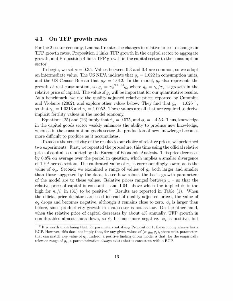
growth rates across capital goods, and it is of interest to see how these translateinto differences in sectoral parameters. For these results, we use the benchmarkvalue of gq = 1.026 based on Cummins and Violante (2002). Jorgenson et al (2005)report TFP growth measures for several capital goods industries. However, it is notclear that their methodology of TFP measurement allows these figures to be mappeddirectly into the current framework.13 Instead, we impute TFP growth rates usingLemma 1, which implies a relationship between relative prices and relative TFP.Cummins and Violante (2002) also provide data on the quality-adjusted relativeprice of capital for a comprehensive list of durable good types, which can be used tocompute the long-run TFP growth rate for that good implied by Lemma 1.14
Results are reported in Table (2). Based on relative prices, TFP growth ratesacross capital types range from 20% for computers and office equipment to 1.3% forstructures. Thus, the model economy is consistent with a wide dispersion of TFPgrowth rates. A prediction of the model (and of many multi-sector models) is thatchanges in the relative prices of goods should be related to the TFP growth ratesof the sectors that produce those goods, as measured by other methods. Hence,Table (2) also reproduces the TFP growth rates from Jorgenson et al (2005), for theperiod 1960 − 2004, and compares them to the TFP growth rates implied by themodel and the relative prices. It is to be expected that the values generated by themodel are higher: the price data used to compute model TFP are quality-adjusted,whereas Jorgenson et al (2005) do not adjust for improvements in output quality.Nonetheless, the correlations between the two series are high: 91% for the full series,and 60% if one excludes Computers and Office Equipment, which is an outlier inboth cases. The Spearman rank correlation is a remarkable 62%.Values of φi in Table 2 are below unity for all sectors. The data are consistent
with a wide distribution of values of φi across different types of capital good whencompared to the value of φx for the "aggregate" capital sector in Table 1. Inter-estingly, all capital goods industries appear to be more "fertile" than non-durableswhen compared to φc in Table 1.
15
13In particular, Jorgenson et al (2005) account for intermediate goods in their measurementstrategy, whereas the current model lacks intermediate goods.14TFP estimates are based on relative prices of capital goods (adjusted for quality following
Gordon (1990)) and the benchmark value of γs. See Cummins and Violante (2002) for details on theconstruction of the price indices. In Table 2, industries are aggregated to yield a consistent partitionbetween the classifications used by the two sources — using the BEA investment expenditure sharesfor the price data, and Domar weights for the JHS data. We are grateful to Gianluca Violante forproviding us with relative price data.15In a more disaggregated industry classification we find that only one category — Agricultural
Machinery excluding Tractors — is less fertile than the consumption sector.
18

Capital good sector γMODELi φi γJHS
i
Computers and office equipment 20.15 0.84 10.40Communication equipment 9.66 0.69 1.24Aircraft 8.82 0.66 0.74Instruments and photocopiers 6.29 0.53 1.17Autos and trucks 3.50 0.17 0.29Fabricated metal products 3.32 0.13 0.56Electrical transm. distrib. and industrial appl. 3.22 0.10 0.55Other 2.98 0.03 0.51Ships and boats 2.67 −0.08 0.45Machinery 2.58 −0.12 0.19Electrical equipment, n.e.c. 2.51 −0.15 0.83Mining and oilfield machinery 1.89 −0.52 −0.16Furniture and fixtures 1.66 −0.73 0.89Structures 1.34 −1.14 −1.05Table (2) — Total factor productivity growth γi in the model, based on the quality-
adjusted price of capital (Cummins and Violante (2002)). We also report TFP
values from Jorgenson et al (2005) (JHS). The Spearman rank correlation is 62%.
4.2 On R&D intensities
We now turn to the quantitative implications of the model for R&D intensity in the2-sector case. According to (31), this requires calibrating three additional parame-ters: δT , σx and σc. In the model, R&D is any activity that increases TFP. Thus,the empirical counterpart of Li in the data includes not just research scientists buteveryone whose function is to complement and support their research activities ratherthan the production of final goods and services, e.g. their laboratory assistants, ad-ministrative staff, sanitation and security service providers, etc. It could also includethe labor of people not occupied in research institutions if their activities add tothe accumulation of knowledge, such as certain management, marketing, and otheractivities.16 Thus, the empirical counterpart of model R&D employment probablyinvolves "much more" than the numbers reported by the NSF. Still, although direct
16For example, in quality-adjusted terms, an activity that identifies that a certain scent or colorof soap is more valued by customers than another might be considered TFP-enhancing, caeterisparibus.
19

comparison may be difficult, our results are suggestive as to the relative importanceof different parameters.
δT = 0.0 0.01 0.05 0.1 0.2 0.3R&D intensity, c 7.6 11.4 13.9 14.6 14.9 15.1R&D intensity, x 32.7 35.9 42.3 45.5 48.1 49.2
σx = 0.0 0.2 0.4 0.6 0.8 1.0R&D intensity, c 7.6 7.6 7.6 7.6 7.6 7.6R&D intensity, x 32.7 32.5 32.3 32.2 32.0 31.9
σc = 0.0 0.2 0.4 0.6 0.8 1.0R&D intensity, c 7.6 8.1 8.8 9.5 10.4 11.5R&D intensity, x 32.7 32.7 32.7 32.7 32.7 32.7
Table (3) — R&D intensity: Sensitivity to δT , σx and σc.
Results assume that all paremeters but the one of interest
are set to their benchmark values — however, this is
without loss of generality since R&D intensity in any given
sector does not depend on spillovers in other sectors.
We will study several different values. Nonetheless, a benchmark is required.Nadiri and Prucha (1996) estimate depreciation rates for knowledge of 12%, andPakes and Schankerman (1984) find values up to 25%. However, these are all mea-sures of the economic depreciation of ideas and, as with capital, this is distinct from"physical" depreciation. Consequently, the value of δT in the model is likely to beconsiderably smaller. Indeed, while the notion of "physical" depreciation is easy tointerpret for the case of capital, the same is not the case for knowledge. We useδT = 0 as a benchmark. Estimates of cross-industry R&D spillovers that might beuseful for calibrating σi exist only for the manufacturing sector, and mostly for asubset of industries that are responsible for the bulk of reported R&D. Nonetheless,Schultz (2006) finds that statistically significant spillovers do not exist for most man-ufacturing industries. Adams and Jaffe (1996) also argue that spillovers are unlikelyto be a significant source of returns to R&D. We select σx = 0 and σc = 0 as abenchmark.The sensitivity of R&D intensity to δT , σx and σc is displayed in Table (3). Raising
δT increases the increases the R&D intensity of both sectors as larger R&D invest-ments are required for given rates of productivity growth. The spillover parametershave far less impact on R&D intensity. Their impact is consistent with Proposition
20

5: however, the primary determinant of R&D intensity appears to be φi, not σi.Thus, in the model economy, TFP growth rates and R&D intensity may be highlycorrelated in cross-section, because they are both primarily determined by φi andnot because there is any causal relationship between them. Indeed, Wilson (2002)finds that R&D intensity is indeed related to the decline in the quality-adjusted priceof capital goods in industry cross-section — which in the current model is indicativeof relative TFP growth differences.
5 More on the Knowledge Production Function
5.1 Fertilization across sectors
A central result of the paper is that, in the model economy, long run differencesin TFP growth persist only to the extent to which industries differ in terms ofknowledge fertility φi. The model economy, however, assumes that there are noknowledge spillovers across sectors. Can differences in TFP growth rates persisteven when such "cross fertilization" is allowed for, and might other parameters havea role to play when such spillovers are possible?Suppose for simplicity that there are two sectors i and j in the model economy.
The production function for knowledge is:
Fiht = AiTφijjt
¡T 1−σiiht T σi
it
¢φi QαihtL
1−αiht (32)
This is the same as (8), except that now it is possible for knowledge in sector i toinfluence sector j, and vice-versa. φij is the extent to which sector i benefits fromknowledge produced in sector j. In this case, deriving the properties of a balancedgrowth path yields the following results:
Proposition 6 Proposition 1 holds when Φ is replaced by
Φ1 =
∙1− φx − φxc
µ1− φx + φcx1− φc + φxc
¶− α
1− α
¸−1(33)
Proposition 7 Along the balanced growth path, sectoral TFP growth rates satisfythe condition
γ1−φc+φxcc = γ1−φx+φcxx (34)
Thus, if γc ≥ 1, then γx ≤ γc if and only if φx + φxc ≥ φc + φcx.
21

It remains the case that differences in TFP growth rates are related only tothe fertility parameters. What matters is no longer simply the "self-fertilization"parameter, but the sum of all the fertility parameters that benefit a given sector, re-gardless of which industry generates the knowledge. When industry cross-pollinationis allowed for, the aggregate growth rate may depend upon fertility parameters otherthan those in the durables sector, but only to the extent to which durable goodsbenefit from knowledge produced in other industries. This is because there is an ex-tra channel whereby the production of knowledge pertaining to durables may benefitthat sector, via feedback through knowledge production in non-durables.
5.2 Duplication in research
We next consider the possibility of duplication in research, i.e. the knowledge pro-duction function may not be constant returns to rivalrous inputs:
Fiht = Ai
¡T 1−σiiht T σi
it
¢φi £QαihtL
1−αiht
¤ψi (35)
where ψi is the returns to rivalrous inputs in sector i. This departs from the em-pirical literature in that the stock of R&D spending no longer measures the stock ofknowledge.
Proposition 8 Proposition 1 holds when Φ is replaced by
Φ2 =
µ1− φxψx
− α
1− α
¶−1, (36)
where ψx ≡Pz
j=m
ψjκj(1−φx)1−φj
is a weighted average of ψj in the capital-producingsectors.
Proposition 8 is identical to Proposition 1 if we replace (1− φx) by (1− φx) /ψx.As in Proposition 1, the only restriction on fertility is on the capital goods sector.The value of φx is still bounded away from unity due to the role of capital in theknowledge production function, but this bound is less strict when there is duplicationin research in the "aggregate" capital sector (ψx < 1). Note that Jones (1995) alsoallows for ψ < 1, in fact our relationship γx = gΦ2N is identical to that of Jones (1995)if α→ 0. However, by assuming away capital in the knowledge production function,Jones’ restriction is independent of ψ. Therefore allowing capital to be an input intothe production of ideas not only implies that Jones’ restriction is not sufficient (as wediscuss in Proposition 1), but it also implies that the degree of diminishing returnsalso matters for the restrictions required by constant aggregate growth.
22

Proposition 9 Along the balanced growth path, sectoral TFP growth rates satisfythe condition
γ1−φiψi
i = γ
1−φjψj
j (37)
Thus, for any two sectors i, j with γi, γj ≥ 1, we have
γi ≥ γj if and only ifψi
1− φi≥
ψj
1− φj. (38)
Proposition 8 is identical to Proposition 1 if we replace 1−φiψi
with 1 − φi. Thederminant of long run differences in TFP growth rates is still the fertility parameter,now adjusted by the degree of returns to rivalrous inputs. Observe that, if ψi takessimilar values across sectors, the range of fertility values that are consistent with thedata does not depend on the value of ψi itself.
6 Concluding remarks
We develop a multi-sector endogenous growth model in which technical progress isdriven by the production of new knowledge. The model is specified so that theproduction functions for goods and for knowledge are close to those estimated inthe empirical literature. In the model, we find that the only long-run determinantof productivity growth differences across sectors is the parameter which dictates theextent of decreasing returns to pre-existing knowledge in the production of new ideas— the extent to which knowledge is fertile. Although this parameter has not beenidentified as a potentially important source of cross-industry differences, it turnsout to play a pivotal role in general equilibrium, and a contribution of our paperis to study the behavior of an economy in which this parameter may differ acrossindustries. Moreover, the restriction on this parameter that determines the existenceof a balanced growth path applies only to the fertility of knowledge in the capitalgoods sector, so that very large or very small intertemporal returns to knowledge "onaverage" may be consistent with balanced growth.Our growth model attempts to take into account a number of factors that growth
theorists and researchers of R&D have independently thought to be of potentialimportance to productivity change and R&D intensity. Interestingly, we find thatinter-sectoral differences in productivity and R&D activity cannot be driven by mostof those factors. Whether or not improvements in the quality of measures of knowl-edge eventually allow empirical work to confirm or reject this prediction, we suspect
23

that any apparent tension between general equilibrium theories of growth and theo-ries of R&Dmay lie in the nature of models of knowledge that underlie these theories.The rigorous formulation and testing of different theories of the way economicallyuseful knowledge is produced, stored and disseminated remains a fertile area forfuture research.Given the centrality of the fertility for knowledge, φi, one may ask what are its
determinants. Nelson andWinter (1977) argue that innovations often follow "naturaltrajectories" that have a technological or scientific rationale rather than being drivenby movements in demand. Similarly, Rosenberg (1969) talks of innovation followinga "compulsive sequence." In a general equilibrium framework, demand plays an es-sential role in providing incentives to innovate: however, in our model the primarydeterminant of long run growth rates is the usefulness or relevance of past knowledgefor the generation of new ideas, something that is reminiscent of these "natural tra-jectories" since it is leads to parametrically determined long-run TFP growth rates.Mokyr (2002) suggests a nuanced view of knowledge, whereby there is a distinctionbetween the set of techniques that are known and the epistemic knowledge that un-derlies them. Perhaps φi reflects differences in the structure of the feedback betweenthe techniques suggested by new epistemic knowledge and the epistemic knowledgethat is generated by the application or refinement of new techniques. Furman andStern (2006) identify the notion of "cumulativeness," which is related to the institu-tions that allow scientists access to preexisting knowledge. Although it is unclear apriori whether cumulativeness is related to φi, Ai, or both, this suggests that study-ing the networks that underlie the storage and transition of knowledge may be useful,and that there may be institutional dimensions to the value of φi. This raises po-tentially interesting policy questions.17 In all, a theory of φi could be an interestingextension of the paper.
17The Jones (1995) result that decreasing returns to knowledge were required for a BGP in thepresence of population growth was originally interpreted as ruling out the possibility of policyimpacting growth. However, if this is itself an institutional parameter, then policies that, forexample, enhance the density of the network of scientists may have a role to play in determininglong run growth rates.
24

7 Bibliography
Abdih, Yasser and Joutz, Frederick. "Relating the Knowledge Production Functionto Total Factor Productivity." International Monetary Fund Staff Papers, 53 (2)(2006), 242-71.Acemoglu, Daron andGuerrieri, Veronica. "Capital Deepening and Non-Balanced
Economic Growth." Mimeo: MIT 2006.Adams, James D.; Jaffe, Adam B. "Bounding the Effects of R&D: An Investiga-
tion Using Matched Establishment-Firm Data." RAND Journal of Economics, Vol.27, No. 4. (Winter, 1996), pp. 700-721.Aghion, Philippe & Howitt, Peter, 1992. "A Model of Growth through Creative
Destruction," Econometrica, 60(2), pages 323-51.Bernstein, Jeffrey I. and Nadiri, Ishaq. "Interindustry R&D Spillovers, Rates of
Return and Production in High-Tech Industries." American Economic Review, 78(1988): 429-34.Bernstein, Jeffrey I. and Nadiri, Ishaq. "Research and Development and In-
traindustry Spillovers: An empirical Application of Dynamic Duality." Review ofEconomic Studies, 56 (1989): 249-269.Burnside, Craig, 1996. "Industry innovation: where and why A comment,"
Carnegie-Rochester Conference Series on Public Policy, Elsevier, vol. 44, pages 151-167.Cohen, Wesley M., Levin, Richard C. "Empirical studies of innovation and market
structure." R. Schmalensee & R. Willig (ed.) Handbook of Industrial Organization,, chapter 18, pages 1059-1107, 1989. Elsevier.Cohen, Wesley M., Levin, Richard C.; Mowery, David C. "Firm Size and R & D
Intensity: A Re-Examination." Journal of Industrial Economics 35(4), The EmpiricalRenaissance in Industrial Economics (Jun., 1987), pp. 543-565.Cummins, Jason and Violante, Giovanni. "Investment-Specific Technical Change
in the US (1947-2000): Measurement and Macroeconomic Consequences." Review ofEconomic Dynamics 5(2), April 2002, 243-284.Jeffrey L. Furman, Scott Stern. "Climbing Atop the Shoulders of Giants: The
Impact of Institutions on Cumulative Research." NBER Working Paper No. 12523,September 2006.Gordon, Robert J. "TheMeasurement of Durable Goods Prices." National Bureau
of Economic Research Monograph. University of Chicago Press, 1990.Greenwood, Jeremy, Hercowitz, Zvi and Krusell, Per. "Long-Run Implications
of Investment-Specific Technological Change", American Economic Review, 87 (3)(1997) 342-62.
25

Griliches, Zvi. "Patent Statistics as Economic Indicators: A Survey" Journal ofEconomic Literature, 28(4). (1990) 1661-1707.Jaffe, Adam B. "Technological Opportunity and Spillovers of R & D: Evidence
from Firms’ Patents, Profits, and Market Value." American Economic Review, Vol.76, No. 5 (Dec., 1986), pp. 984-1001.Jones, Benjamin F. “The Burden of Knowledge and the Death of the Renais-
sance Man: Is Innovation Getting Harder?” Mimeo: Kellogg School of Management,Northwestern University, 2005b.Jones, Charles. "R&D-Based Models of Economic Growth." Journal of Political
Economy 103 (1995) 759-84.Jones, Charles. "Sources of U.S. Economic Growth in a World of Ideas." Ameri-
can Economic Review 92 (2002) 220-239.Jones, Charles. "Ideas and Growth." in P. Aghion and S. Durlauf (eds.) Hand-
book of Economic Growth (Elsevier, 2005a) Volume 1B, pp. 1063-1111.Jorgensen, Dale, Mun S. Ho, and Kevin J. Stiroh. "Information Technology and
the American Growth Resurgence." In: Jorgensen, Dale, Mun S. Ho, Jon Samuelsand Kevin J. Stiroh, Eds. Industry Origins of the American Productivity Resurgence.Cambridge, The MIT Press, 2005.Kaldor, Nicholas. “Capital Accumulation and Economic Growth.” in Friedrich
A. Lutz and Douglas C. Hague, eds., The Theory of Capital. New York: St. Martin’sPress, 1961, 177-222.Klenow, Peter J. "Industry Innovation: Where and Why," Carnegie-Rochester
Conference Series on Public Policy 44, June 1996, 125-150.Kortum, Samuel S. "Research, Patenting, and Technological Change." Econo-
metrica, 65, No. 6. (1997), pp. 1389-1419.Krusell, Per. "Investment-Specific R&D and the Decline in the Relative Price of
Capital", Journal of Economic Growth, 3 (1998) 131-141.Lanjouw, Jean and Mark Schankerman (1999) The Quality of Ideas: Measuring
Innovation with Multiple Indicators." NBER Working Paper w7345.Mokyr, Joel. The Gifts of Athena: Historical Origins of the Knowledge Economy.
Princeton: Princeton University Press, 2002.Nadiri, M. Ishaq; Prucha, Ingmar R. "Estimation of the Depreciation Rate of
Physical and R&D Capital in the U.S. Total Manufacturing Sector." Economic In-quiry 34 (1996) 43-56.Nelson, Richard R., Winter, Sidney. "In search of useful theory of innovation."
(sic) Research Policy, 1993, 6, 36-76.Pakes, Ariel; Schankerman, Mark. "An Exploration into Determinants of Re-
search Intensity."; R&D, Patents, and Productivity, NBERConference Report. Chicago
26

and London: University of Chicago Press (1984) 209-232.Porter, Michael E. and Stern, Scott. "Measuring the "Ideas" Production Func-
tion: Evidence from International Patent Output." NBER Working Paper w7891(2000).Romer, Paul. "Endogenous Technological Change." Journal of Political Economy
98 (1990) S71-S101.Rosenberg, Nathan. (1969) "The direction of technological change: Inducement
mechanisms and focusing devices." Economic Development and Cultural Change,18:1-24.Samaniego, Roberto. "R&D and Growth: the Missing Link?" Macroeconomic
Dynamics (in press).Schultz, Laura I. "Estimating the Returns to Private Sector R&D Investment."
Mimeo: Bureau of Economic Analysis 2006.Vourvachaki, Evangelia. "Information and Communication Technologies in a
Multi-Sector Endogenous Growth Model." Mimeo: London School of Economics,2006.Wilson, Daniel J. "Is Embodied Technology the Result of UpstreamR&D? Industry-
Level Evidence," Review of Economic Dynamics 5 (2002) 285-317.
27

A Derivations
A.1 Household maximization
We first determine the optimal spending across different goods taken as given thetotal per capita spending on consumption sc and total spending on investment sx.Omitting time subscript, the maximization problems across goods are
max{cih}
c s.t. sc =m−1Xi=1
Z 1
0
pihcihdh, and
max{xjh}
x s.t. sx =zX
j=m
Zpjhxjhdh
where c and x are defined in the household problem. The optimal spending withinsectors i = 1, ..m− 1, across different varieties h, isµ
cihcih0
¶−1μi
=pihpih0
=⇒ cih0 = cih
µpihpih0
¶μi
(39)
which implies
ci =
µZ 1
0
cμi−1μi
ih0 dh0¶ μi
μi−1
= cih
"Z µpihpih0
¶μi−1dh0
# μiμi−1
(40)
Using (40), define price index, pi ≡ pihcihdh
ci=hR
p1−μiih dh
i1/(1−μi). We can now
rewrite (40) as ci = cih³pihpi
´μi. Across good i, Cobb-Douglas utility yields pici
pjcj= ωi
ωj,
so pici = ωisc, together with utility function,
pc ≡scc=
m−1Qi=1
pωii (41)
and the demand for good ih is
cih = sc
µpipih
¶μωi
pi(42)
The result follows analogously for investment,
xjh = sx
µpjpjh
¶μjµκjpj
¶and xj = sx
µκjpj
¶, (43)
28

where pj is analogously defined as before, and
px ≡sxx=
zQj=m
pκjj (44)
Given the solution of the static maximization, the dynamic problem is
max{ct,xt}
∞Pt=0
(βgN)t u (ct)
s.t.
pctct + pxtxt = wt +Rtkt + πt
gNkt+1 = xt + (1− δk) kt
The solution implies
u0 (ct)
βu0 (ct+1)=
pxt+1/pct+1pxt/pct
µ1− δk +
Rt+1
pxt
¶(45)
A.2 Firm’s maximzation
The firm’s maximization problem is
max{Nit,Kit,Qit,Lit}
∞Pt=0
λtΠiht
pcts.t.
Tiht+1 = fiht + (1− δT )Tiht
Yiht = Ntciht if i = 1, ..m− 1Yiht = Ntxjht if i = m, ...z
Given Πiht in (10), the static efficiency conditions are standard:
∂Yiht/∂Niht
∂Yiht/∂Kiht=
wt
Rt=
∂fiht/∂Liht
∂fiht/∂Qiht
The assumptions on production functions imply so, for any two sectors i, j, Kiht/Niht =
Qiht/Liht, and piht³1 +
Yjhtpjht
∂pjht∂Yjht
´Tiht = pjht
³1 +
Yjhtpjht
∂pjht∂Yjht
´Tjht. Using the demand
function, relative prices ispihtpjht
=Tjht
¡1− 1/μj
¢Tiht (1− 1/μi)
(46)
29

The dynamic efficiency condition involves the optimal R&D decision. The first ordercondition of the Lagragian with respect to Tiht+1 is
λt+1pct+1
∂Πiht+1
∂Tiht+1− χiht + χiht+1
µ∂fiht+1∂Tiht+1
+ 1− δT
¶= 0 (47)
where
χiht =
µλtpct
¶Rt
∂fiht/∂Qiht(48)
is the shadow price for Tiht+1.
A.3 Market Equilibrium
The capital market clearing condition (11) and equal capital-labor ratios (49) imply
Kiht
Niht=
Qiht
Liht=
K
N= k, and (49)
Rt = αpihtTihtkα−1t
µ1− 1
μi
¶; wt = (1− α) pihtTihtk
αt
µ1− 1
μi
¶. (50)
together with χit in (48), dynamic equation (47) becomes
λtpiht/pctλt+1piht+1/pct+1
ÃTiht¡
T 1−σiiht T σiit
¢φi!
(51)
= Aikαt+1Niht+1 +
Tiht+1¡T 1−σiiht+1T
σiit+1
¢φiµφi (1− σi)
Fiht+1
Tiht+1+ 1− δT
¶We now focus on the symmetric equilibrium across h within i.
B Proofs
Proof of Lemma 1. See the derivation of (49) and (46) in the Firm’s maximization.
Proof of Lemma 2. Define Tx such that:
Ntx ≡ Tx
µzP
i=m
Kit
¶αµ zPi=m
Nit
¶1−α= Txk
αzP
i=m
nit
30

where the equality follow from (49). To determine Tx, (43) impliespjTjk
αnjpiTikαni
=κjκiand,
by (46), niκi=³1−1/μi1−1/μj
´njκj, so
zPi=m
nit =nj (1− 1/μx)κj¡1− 1/μj
¢ (52)
where we define μx such that
1− 1
μx=
zPi=m
κi
µ1− 1
μi
¶⇔ 1
μx=
zPi=m
κiμi
(53)
By definition, x =zQ
j=m
³xjκj
´κj=
zQj=m
³Tjkαnj
κj
´κj, so using (52) and (53), we obtain
x = kαµ
zPi=m
nit
¶zQ
j=m
∙Tj
µ1− 1/μj1− 1/μx
¶¸κjso the index of knowledge is
Tx =
"zQ
j=m
µ1− 1/μj1− 1/μx
¶#zQ
j=m
Tκjj . (54)
Proof of Lemma 3. The Euler condition follows from (45) in the Consumer’sMaximization. Using (44) and (46),
pxpi
=zQ
j=m
µpjpi
¶κj
=zQ
j=m
ÃTi (1− 1/μi)Tj¡1− 1/μj
¢!κj
= Ti (1− 1/μi)zQ
j=m
£Tj¡1− 1/μj
¢¤−κj ∀i,
so by (54), we havepxpi=
Ti (1− 1/μi)Tx (1− 1/μx)
∀i, (55)
together with (50), we have
R
px=
αpiTikα−1
³1− 1
μi
´px
= αkα−1Tx
µ1− 1
μx
¶,
31

so the expression for G follows from its definition.Proof of Lemma 4. Euler equation (45) implies
λt+1λt
=1
1 + rt+1=
βu0 (ct+1)
u0 (ct)=
pxt/pctGt+1pxt+1/pct+1
(56)
Using (55), pxt+1/pit+1pxt/pit
= γiγx, substitute into (51),result follows for (19).
Lemma 5 The equilibrium employment shares for production are
ni = ωic/q
Txkα
µ1− 1/μi1− 1/μx
¶∀i < m, (57)
nj =1− μj1− μx
κj
ÃzP
j=m
njt
!∀j ≥ m. (58)
If positive, the R&D intensity of the firm satisfies
nit+1lit+1
=Gt+1γ
φiit /γxt − (1− δT )
γit+1 − (1− δT )− φi (1− σi) ∀i. (59)
Proof. Combine (19) with (7) to derive ni/li. To obtain ni, use market clearingand the expenditure share of good i = 1, ..m − 1, piTikαni = pici = ωipcc, and soni = ωi
c/qkα
³pxTipi
´where q = px/pc. The result for ni follows from (55). The proof
for nj , j = m..z is analogous.
Proof of Proposition 1. Define ket = ktT−1/(1−α)xt . Let gx ≡ xt+1/xt for all
variables x. From the Euler condition (17), gc is constant if gq and G are constants.From (18), G is constant if and only if ke is constant. Use Lemma 2 and (49) to
rewrite the capital accumulation equation as gNgk = kα−1et
zPj=m
njt + 1− δk, it follows
that gk is constant if and only ifzP
j=m
njt is constant. So (58) implies nj are constants
for j = m, ..z. By defintion, ke is constant if and only if gk = γ−1/(1−α)x , which by (15)
is constant if and only if γj are constants for all j = m, ..z, which is true by (19) ifand only if
Ajkαt+1Njt+1T
φj−1jt+1 = Ajk
αet+1T
α/(1−α)x njt+1Nt+1T
φi−1jt+1
is constant. Given {nj}j=m,..z are constants, we must have ∀j ≥ m,
γα/(1−α)x gNγφi−1j = 1 (60)
32

which implies ∀i, j ≥ m,
γφi−1i = γ
φj−1j , (61)
so γx =zQ
j=m
γκjj =
zQj=m
³γφi−1i
´κj/(φj−1), so ∀j ≥ m,
γ1−φxx = γ1−φii , (62)
where φx satisfies (1− φx)−1 =
zPj=m
κj¡1− φj
¢−1. Thus, (60) implies
γ∗x = gΦN , (63)
where Φ = (1− φx − α/ (1− α))−1 . Finally we need to show gq is constant, using(41),
q−1 =m−1Qi=1
µpxpi
¶ωi
=m−1Qi=1
µTi (1− 1/μi)Tx (1− 1/μx)
¶ωi
, (64)
So gq is constant if and only if γi are constants. From (57), ni are constants fori < m. Using (19) for i < m, γi is constant if and only if (60) holds for i < m aswell. Therefore, (61) holds for i < m as well. Use (49) to rewrite (7) as γit+1 =AiT
φi−1i Nt+1k
αt lit + 1− δT . This is constant from (60). li is constant from (59).
Proof of Proposition 2. The transversality conditions are: limt→∞
ζtkt+1 = limt→∞
χitTit+1 =
0, ∀i. χit and ζt are the corresponding shadow values. From the Firm’s maximizationand (55), we have
χitχit−1
=λtpxt/pct
λt−1pxt−1/pct−1
µγxγi
¶γ1−φii =
1
G
µγxγi
¶γ1−φii
where the last equality follows from (56). Using (17), 1/G = βg1−θc γ−1/(1−α)x , together
with (62),
limt→∞
χitTit+1 = χi0Ti0 limt→∞
£βg1−θc γ−α/(1−α)x γ1−φxx
¤t= χi0Ti0 lim
t→∞
¡βgNg
1−θc
¢twhere the last equality follows from (63). Using (64) and (61),
gq = γ(1−φx)/(1−φc)−1x (65)
where φc satisfies 1/ (1− φc) =Pm−1
i ωi/ (1− φi) . So gc = gqγ1/(1−α)x = γΥx , where
Υ ≡ 1−φx1−φc
+ α1−α . TVC for Ti holds if β < min
¡1/gN , β̄
¢, where β̄ ≡ (1/gN)1+(1−θ)ΦΥ .
33

The lagragian multiplier for k is the discounted marginal utility, ζt = (βgN)t³pxtpct
´u0 (ct) ,
so limt→∞
ζtkt = limt→∞
(βgN)t³qktct
´c1−θt . Since qk/c is constant, TVC for k holds if
and only if β < min¡1/gN , β̄
¢. Finally, we derive conditions for positive li and
ni. From (7), li > 0 if and only if γi > 1 − δT , using (62) and (63), we have
gΦ/(1−φi)N > (1− δT )
1/(1−φx) . >From (19), ni > 0 if and only ifhGφii /γx − (1− δT )
i−
φi (1− σi) [γi − (1− δT )] . Using (60) and (17)
Gγφi−1i
γx=
Gγφx−1x
γx=
γφx−1x
βg1−θc γ−1/(1−α)x γx
=¡βgNg
1−θc
¢−1(66)
where the last equality follows from (25). So Gφi−1i /γx > 1 given β < β̄. A sufficient
condition for ni > 0 is φi (1− σi) < 1.Proof of Proposition 3. Using (12) and (57),
y
c=
pxTxkα
cpc
zPi=1
1− 1/μx1− 1/μi
ni =qk
ckα−1e
zPi=1
1− 1/μx1− 1/μi
ni =⇒c
y=
Pm−1i=1 ni/ (1− 1/μi)Pzi=1 ni/ (1− 1/μi)
which is constant given ni are constants. Using (50), the R&D expenditure share isPzi=1 (Liw +QiR)Pzi=1 piTiK
αi N
1−αi
=(1− 1/μx) pxTxkα
Pzi=1 Li
pxTxkαPz
i=11−1/μx1−1/μi
Ni
=
Pzi=1 liPz
i=1 ni/ (1− 1/μi).
Finally, the real interest rate is constant from (56).Proof of Proposition 4. Condition (29) follows from (26), which implies γi/γj =
γ(φi−φj)/(1−φi)j . By (26) γi ≥ 1 if φi ≤ 1 ∀i. Together they imply: if γi, γj ≥ 1, then
γi ≥ γj if and only if φi ≥ φj.Proof of Corollary 2. See derivation of (65) in proof for Proposition 1.Proof of Proposition 5. From (31),
nili− nj
lj=
(Gγ
φii /γx−(1−δT )γi−(1−δT )
− Gγφjj /γx−(1−δT )γj−(1−δT )
+φj (1− σj)− φi (1− σi)
). (67)
By (60), the first part of the difference becomes
Gγφx−1x
³γiγx
´− (1− δT )
γi − (1− δT )−
Gγφx−1x
³γjγx
´− (1− δT )
γj − (1− δT )
34

=Gγ
φx−1x
³γjγx
´+ γi −Gγ
φx−1x
³γiγx
´− γx
[γi − (1− δT )]£γj − (1− δT )
¤ (1− δT )
=
³Gγ
φx−1x /γx − 1
´ ¡γj − γi
¢[γi − (1− δT )]
£γj − (1− δT )
¤ (1− δT )
From (66) we have Gγφx−1x /γx > 1, so the first part of (67) is positive if and only ifγj > γi. When γi, γj ≥ 1, condition (60) implies γj ≥ γi if and only if φj ≥ φi. Thesecond part of (67) is positve if and only if φj (1− σj) ≥ φi (1− σi).Proof of Propositions 6 and 7. Since Tj is taken as given by firm ih, in termsof the firm dynamic optimization, we just need to replace previous Ai with the termTφijjt Ai, which now depends on t. Firm’s optimal condition (51) becomes
T1−φiit λtpit/pct
λt+1pit+1/pct+1
= Tφijjt Aik
αt+1Nit+1 +
ÃTφijjt
Tφijjt+1
!T1−φiit+1
£φi (1− σi)
¡γit+1 − 1 + δT
¢+ 1− δT
¤As in Lemma 4 using (56) and (55), we have for sector x :
Gt+1γφx−1xt = T
φxcct Axk
αet+1nxt+1T
α/(1−α)+φx−1xt+1 Nt+1 (68)
+γ−φxcct
£φx (1− σx)
£γxt+1 − (1− δT )
¤+ 1− δT
¤and for sector c :
Gt+1γφcct
γxt= T
φcxxt Ack
αet+1nct+1T
α/(1−α)xt+1 T
φc−1ct+1 Nt+1 (69)
+γ−φcxxt
£φc (1− σc)
£γct+1 − (1− δT )
¤+ 1− δT
¤Constant γx and γc requires the first term in both (68) and (69) to be constant, i.e.γφxcc γ
α/(1−α)+φx−1x gN = 1 and γ
φcxx γ
α/(1−α)x γ
φc−1c gN = 1. Combining the two equations
γφxcc γφx−1x = γφcxx γφc−1c ⇔ γ1−φx+φcxx = γ1−φc+φxcc , (70)
which implies γx = gΦ1N , where Φ1 =³1− φx − φxc
³1−φx+φcx1−φc+φxc
´− α
1−α
´−1.
35

Proof of Proposition 8 and 9. Lemma 1 − 3 hold as before. Firm’s optimalcondition (51) becomes
Gt+1γitγxt
ÃTit¡
T 1−σiit T σiit
¢φi!k(α−1)(1−ψi)t Q
1−ψiit
= ψiAikαt+1Nit+1 +
Tit+1k(α−1)(1−ψi)t+1 Q
1−ψiit+1¡
T 1−σiit+1 Tσiit+1
¢φiµφi (1− σi)
Fit+1
Tit+1+ 1− δT
¶Using Lemma 1, it simplifies to
Gt+1γφiit
γxt=
⎧⎨⎩ Aikαt+1Nit+1T
φi−1it+1 ψik
(1−α)(1−ψi)t Q
ψi−1it +³
kt+1kt
´α(ψ−1) ³lit+1lit
´1−ψg1−ψiN
£φi (1− σi)
¡γit+1 − 1 + δT
¢+ 1− δT
¤⎫⎬⎭
The restriction for BGP requires the first term to be constant,
Aikαt+1Nit+1T
φi−1it+1 ψik
(1−α)(1−ψi)t Q
ψi−1it
= ψAikαet+1T
α/(1−α)xt+1 nit+1Nt+1T
φi−1it+1 k
α(ψi−1)et T
α(ψi−1)/(1−α)xt l
ψi−1it N
ψi−1t
which is constant if
γα/(1−α)x gNγφi−1i γα(ψi−1)/(1−α)x g
ψi−1N = 1⇔
¡γα/(1−α)x gN
¢ψi γφi−1i = 1 ∀i (71)
so across sectors we have
γφj−1j
γφi−1i
=¡γα/(1−α)x gN
¢ψi−ψj ∀i, j (72)
So γx =zQ
j=m
γκjj =
zQj=m
∙³γα/(1−α)x gN
´ψi−ψjγφi−1i
¸κj/(φj−1), which implies γφx−1x =
γφi−1i
hγα/(1−α)x gN
iψi−ψx, for i ≥ m, where ψx =
Pzj=m
κj(1−φx)1−φj
ψj. Together with
(72)
γφj−1j = γφx−1x
£γα/(1−α)x gN
¤ψx−ψj ∀j (73)
But (71) implies³γα/(1−α)x gN
´ψj= γ
1−φjj , ∀j, substitute into (73),
γ
1−φjψj
j = γ1−φxψx
x ∀j (74)
Substitute back to (71), we have³γα/(1−α)x gN
´ψiγφx−1x
hγα/(1−α)x gN
iψx−ψi= 1, which
implies γx = gΦ2N , where Φ2 =³1−φxψx− α
1−α
´−1.
36

CENTRE FOR ECONOMIC PERFORMANCE Recent Discussion Papers
761 Mariano Bosch Job Creation and Job Destruction in the Presence of Informal Labour Markets
760 Christian Hilber Frédéric Robert-Nicoud
Owners of Developed Land Versus Owners of Undeveloped Land: Why Land Use is More Constrained in the Bay Area than in Pittsburgh
759 William Nickell The CEP-OECD Institutions Data Set (1060-2004)
758 Jean Eid Henry G. Overman Diego Puga Matthew Turner
Fat City: the Relationship Between Urban Sprawl and Obesity
757 Christopher Pissarides Unemployment and Hours of Work: the North Atlantic Divide Revisited
756 Gilles Duranton Henry G. Overman
Exploring the Detailed Location Patterns of UK Manufacturing Industries Using Microgeographic Data
755 Laura Alfaro Andrew Charlton
International Financial Integration and Entrepreneurship
754 Marco Manacorda Alan Manning Jonathan Wadsworth
The Impact of Immigration on the Structure of Male Wages: Theory and Evidence from Britain.
753 Mariano Bosch William Maloney
Gross Worker Flows in the Presence of Informal Labour Markets. The Mexican Experience 1987-2002
752 David Marsden Individual Employee Voice: Renegotiation and Performance Management in Public Services
751 Peter Boone Zhaoguo Zhan
Lowering Child Mortality in Poor Countries: the Power of Knowledgeable Parents
750 Evangelia Vourvachaki Information and Communication Technologies in a Multi-Sector Endogenous Growth Model

749 Mirko Draca Raffaella Sadun John Van Reenen
Productivity and ICT: A Review of the Evidence
748 Gilles Duranton Laurent Gobillon Henry G. Overman
Assessing the Effects of Local Taxation Using Microgeographic Data
747 David Marsden Richard Belfield
Pay for Performance Where Output is Hard to Measure: the Case of Performance Pay for Teachers
746 L Rachel Ngai Christopher A. Pissarides
Trends in Hours and Economic Growth
745 Michael White Alex Bryson
Unions, Job Reductions and Job Security Guarantees: the Experience of British Employees
744 Wendy Carlin Andrew Charlton Colin Mayer
Capital Markets, Ownership and Distance
743 Carlos Thomas Equilibrium Unemployment and Optimal Monetary Policy
742 Tobias Kretschmer Katrin Muehlfeld
Co-Opetition and Prelaunch in Standard Setting for Developing Technologies
741 Francesco Caselli Nicola Gennaioli
Dynastic Management
740 Michael Noel Mark Schankerman
Strategic Patenting and Software Innovation
739 Nick Bloom Stephen Bond John Van Reenen
Uncertainty and Investment Dynamics
738 Sami Napari The Early Career Gender Wage Gap
The Centre for Economic Performance Publications Unit Tel 020 7955 7673 Fax 020 7955 7595 Email [email protected]
Web site http://cep.lse.ac.uk