Embed Size (px)
Citation preview

NOVICE
APPROACH TO
CALCULIX
BY
SRILALITHKUMAR SWAMINATHAN
TEAM 7
EML 5526

CALCULIX:
Calculix is a free and open source finite element analysis package. It consists of
an implicit and explicit solver (CCX) written by Guido Dhondt and a pre and post
processor (CGX) written by Klaus Wittig.
Website:
http://www.calculix.de/
Calculix has an active discussion group on yahoo:
http://groups.yahoo.com/group/calculix/
HOW TO INSTALL CALCULIX:
1. Go to http://www.dhondt.de/
2. Find the link “for a Windows executable: look
at www.bconverged.com/calculix.”
3. click on the link
4. Now you will be taken to taken to a new site.
5. then click on download,
6.

7. 8. Then you will be downloading a file a zip file.
9. Unzip the file
10. Open the folder you will and executable file, run it.

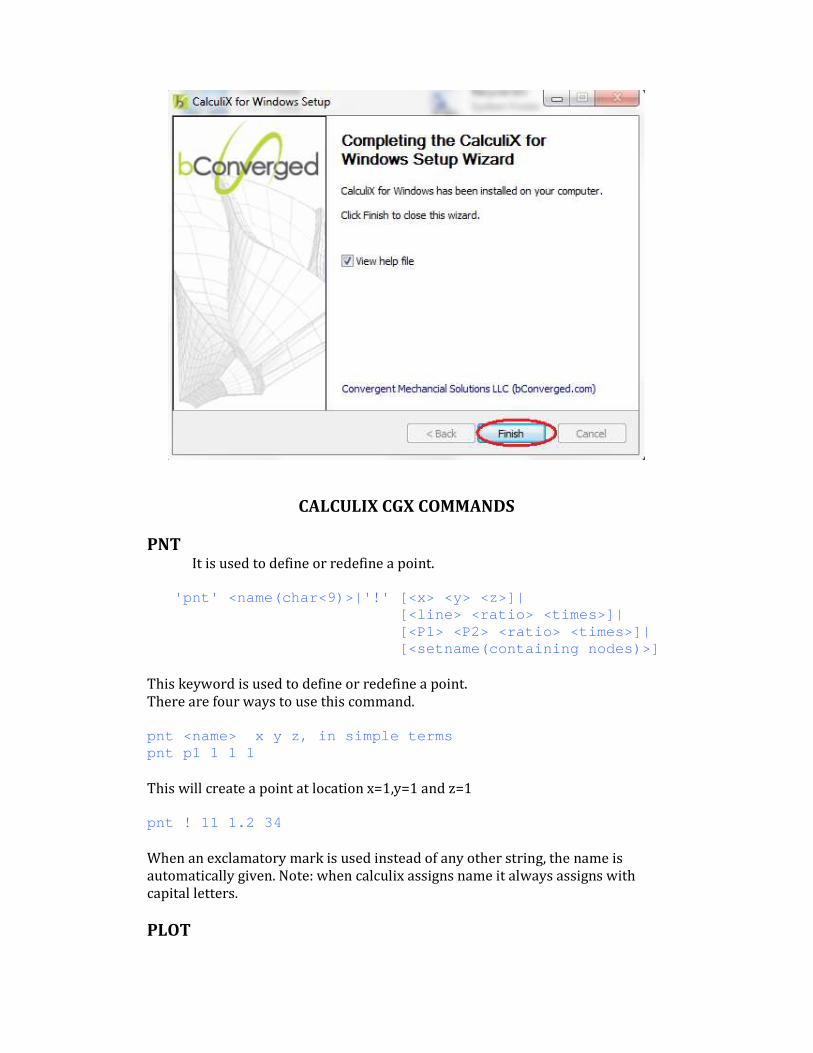
CALCULIX CGX COMMANDS
PNT It is used to define or redefine a point.
'pnt' <name(char<9)>|'!' [<x> <y> <z>]| [<line> <ratio> <times> ]| [<P1> <P2> <ratio> <tim es>]| [<setname(containing no des)>]
This keyword is used to define or redefine a point.
There are four ways to use this command.
pnt <name> x y z, in simple terms pnt p1 1 1 1
This will create a point at location x=1,y=1 and z=1
pnt ! 11 1.2 34
When an exclamatory mark is used instead of any other string, the name is
automatically given. Note: when calculix assigns name it always assigns with
capital letters.
PLOT

'plot' ['n'|'e'|'f'|'p'|'l'|'s'|'b'|'S'|'L']&['a'|'d'|'p'| 'q'|'v'] -> <set> 'w'|'k'|'r'|'g'|'b'|'y'|'m'
This command is used to display the required entities of the model on the CGX
screen and hide any existing entity displayed earlier.
Types of entities
Entity Attribute:Symbol/Syntax
Nodes ‘n’
Elements ‘e’
Points ‘f’
Faces ‘p’
Lines ‘l’
Surfaces ‘s’
Bodies ‘b’
We can also display entities in colours
Colour Attribute:Symbol/Syntax
Red ‘r’
Green ‘g’
Blue ‘b’
Magenta ‘m’
black ‘k
Yellow ‘y’
White ‘w’
Example:
Plot p all will display all points
Plot pa all will display all points with their names
Plot pa all r Will display all points with their names in red
PLUS
Now we might have situations when one or more entity might be needed to be
displayed. But using plot will hide any prevousily displayed entity so we need to
plus command. Plus command is used as a addendum for plot command. In
syntax for plus command is same as plot.
Plot p all will display all points

Plus la all will display all lines with their names but will not remove the points displayed.
LINE 'line' <name(char<9)>|'!' <p1> <p2> <div> This command is used to define or redefine a line segment. A line segment is
defined by a start and end point.
For Example:
line L01 P1 P2 4
The above syntax will create a line with name ‘L01’ with start point ‘P1’ and end
point ‘P2’ with 4 divisions on it.
ELTY 'elty' [<set>] ['be2'|'be3'|'tr3'|'tr3u'|'tr6'|'qu4 '|-> 'qu8'|'he8'|'he8f'||'he8i'|'he8r'|'he20'|'he20r']
This command is used to assign a given element type to a set of entities of the
model. For more regarding the type of elements visit:
http://bconverged.com/calculix/doc/cgx/html/node150 .html or calculiX help file.
The element name is composed of the following parts:
1. The leading two letters define the shape (be: beam, tr: triangle, qu:
quadrangle, he: hexahedra),
2. Then the number of nodes
3. An attribute describing the mathematical formulation
4. Other features (u: unstructured mesh, r: reduced integration, i:
incompatible modes, f: fluid element for ccx).
For example:
Elty all he8 will assign hexagonal elements to all entities
MESH mesh <set>
mesh command is used to begin the meshing of the model, before using the mesh
command, the element types must be defined by using the elty command.
For example:

Mesh all
GSUR 'gsur' <name(char<9)>|'!' '+|-' 'BLEND|<nurbs>' '+| -' <line|lcmb> '+|-' -> <line|lcmb> .. (3-5 times)
This command is used to define or redefine a surface. Each surface must have
three to five lines or combined lines so that it is.
For example,
gsur S001 + BLEND - L001 + L002 + L003 - L004
This will create the surface S001 with a mathematically positive orientation
indicated by the ''+'' sign after the surface name from the lines
L001,L002,L003,L004.
For details regarding BLEND key word please refer help file attached with
calculix. Use a ''+'' or ''-'' in front of the lines to mention the orientation.
GBOD
'gbod' <name(char<9)>|'!' 'NORM' '+|-' <surf> '+|-' <surf> -> .. ( 5-7 surfaces )
gbod command is used to define or redefine a body. Each body must have five to
seven surfaces to be mesh-able. The first two surfaces should be the ''top'' and
the ''bottom'' surfaces.
For example,
gbod B001 NORM - S00A + S00B - S00C - S00D - S00E - S00F
will create a body B001 comprising of surfaces S00A,S00B,S00C,S00D,S00E,S00F.
For details regarding NORM key word please refer help file attached with
calculix. The sign ''+'' or ''-'' in front that indicates the orientation of each surface.
SAVE
'save' This command is used to save the geometry to a file named as the input file with
the extension .fbd.
QLIN 'qlin' <name>(optional) RETURN 'w'|'b'|'c'|'e'|'g'|'l'|'m'|'p'|'q'|'s'|'t'|'u'|'x'

This command is used to create a sequence of lines by allowing the user to pick
points.
Steps involved in Qlin :
type qlin type a wait for command to display “ mode:a ” type r Starting point of the cursor and cursor, now move t he cursor to some other point type r An rectangle is displayed, the size of the rectangl e is controlled by position of the cursor.
Now place the rectangle cursor over the start point and press ‘ b’

Now place the rectangle cursor over the centre poin t and press ‘c’ (only in case of arc) Now place the rectangle cursor over the end point a nd press ‘g’
To quit the qlin command press q Note: By above the name for the line automatically assigned.

CALCULIX CGX MENU COMMANDS:
Open calculix bconverged installation directory,
C:\Program Files\bConverged\CalculiX\ccx\test\ Open beampl.inp file . The file will in open CGX window.
FRAME
Adjusts the model to fit the display window.

Left-click on left pane -> select frame
Similarly all the menu commands can be accessed by left-clicking on the left-
plane
ORIENTATION
Left-click on the left pane->orientation-> [ORIENTA TION OPTIONS] The oreintation option includes ‘+x-axis’ ‘-x-axis’ ‘+y-axis’ ‘-y-axis’ ‘+z-axis’ ‘-z-axis’
VIEWING Left-click on the left pane->orientation-> [VIEWING OPTIONS]
This command is used for selected the entities that are to be displayed.
HARDCOPY Left-click on the left pane->Hardcopy-> [OPTIONS] This command is used to export the calculix window as required image format.
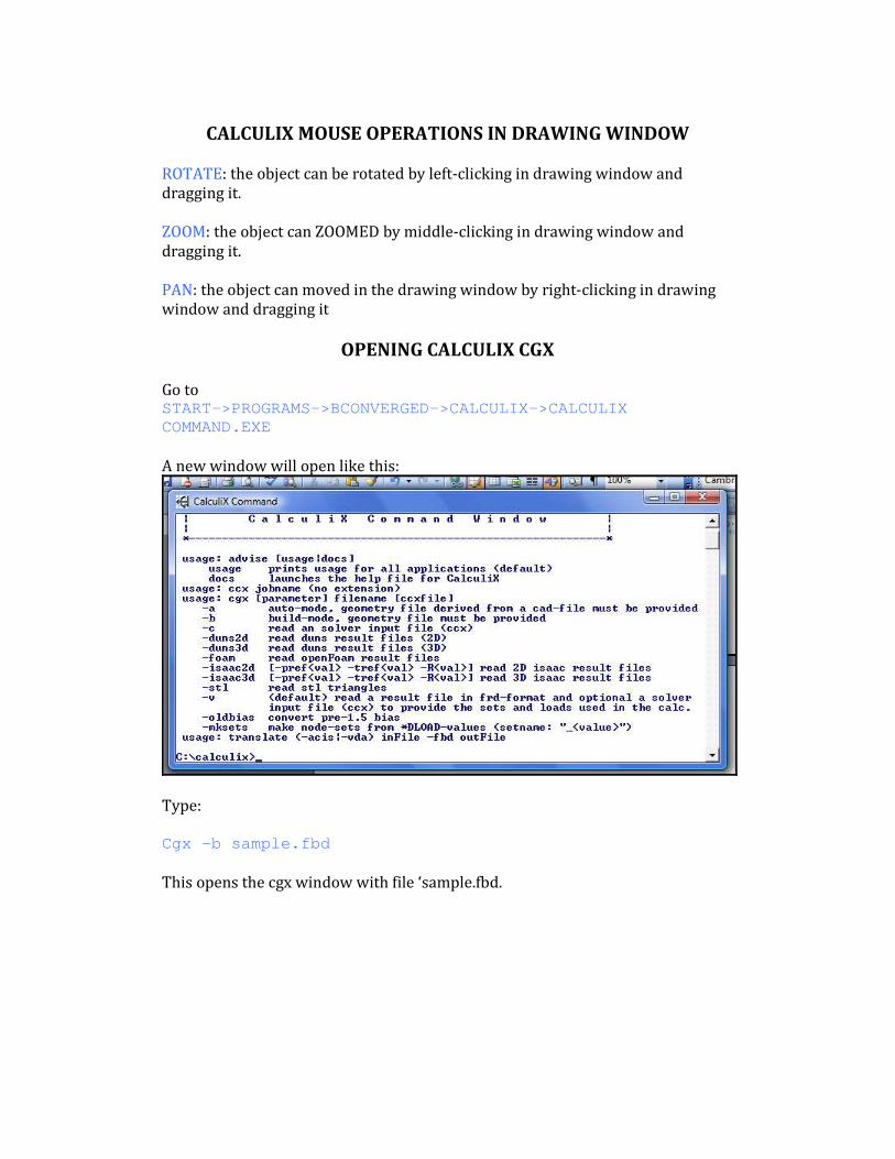
CALCULIX MOUSE OPERATIONS IN DRAWING WINDOW
ROTATE: the object can be rotated by left-clicking in drawing window and
dragging it.
ZOOM: the object can ZOOMED by middle-clicking in drawing window and
dragging it.
PAN: the object can moved in the drawing window by right-clicking in drawing
window and dragging it
OPENING CALCULIX CGX
Go to START->PROGRAMS->BCONVERGED->CALCULIX->CALCULIX COMMAND.EXE
A new window will open like this:
Type:
Cgx –b sample.fbd
This opens the cgx window with file ‘sample.fbd.

Now in order use cgx, the cgx window needs to be active always but the
commands will be visible only in the calculix command window.
Before proceeding to the basic examples:
A small set of codes to try out:
Create four points P1(0,0,0) P2(1,0,0) P3(0,1,0) P4(1,1,0).
Display all the points with labels in magenta.
Create line L001 with points P1, P2
Create line L002 with points P2, P3
Create line L003 with points P1, P3
Create line L004 with points P4, P2
Display on the lines without labels,
Now display points with labels without erasing the displayed lines
From lines L001, L002, L003, L004 make surface S001.
Display only in surface with its name.

The code: PNT P1 0.00000 0.00000 0.00000 PNT P2 1.00000 0.00000 0.00000 PNT P3 0.00000 1.00000 0.00000 PNT P4 1.00000 1.00000 0.00000 Plot pa all m LINE L001 P1 P2 104 LINE L002 P1 P3 104 LINE L003 P3 P4 104 LINE L004 P4 P2 104 Plot l all Plus pa all GSUR S001 + BLEND - L001 + L002 + L003 + L004 plot sa all
The example can also be done with QLIN command
Using Line command for drawing arcs:
Syntax for creating arc using line command
Line <name> <start point> <end point> <centre> <divisioins>
Create five points (0,0,0),(1,0,0),(0,1,0),(-1,0,0),(0,-1,0)
Now join the lines in such a way they form a circle.
The code: pnt p0 0 0 0 pnt p1 1 0 0

pnt p2 0 1 0 pnt p3 -1 0 0 pnt p4 0 -1 0 line l001 p1 p2 p0 4 line l002 p2 p3 p0 4 line l003 p3 p4 p0 4 line l004 p4 p1 p0 4
The example can also be done with QLIN command
Using ‘QADD’ to create a set of entities:
QADD: We will be situation when there is no need display all the lines and
points or surface.
For example consider the following code:
PNT P1 0.00000 0.00000 0.00000 PNT P2 1.00000 0.00000 0.00000 PNT P3 0.00000 1.00000 0.00000 PNT P4 1.00000 1.00000 0.00000 LINE L001 P1 P2 104 LINE L002 P1 P3 104 LINE L003 P3 P4 104 LINE L004 P4 P2 104 Plot pa all Plus la all

Notice the ‘all’ keyword at the end of the plot command. Which is indicates that
all lines and all the lines will be displayed. But assuming we are in situation
where we are need of printing only the lines L001 and L002.
Then instead ‘all’ key word, we use a set name. A set will consists entities such as
lines,points nodes etc. To create a set, we will use QADD command.
Syntax for QADD:
'qadd' <set|seq> 's'|RETURN <'w'|'a'|'i'|'r'|'n'|'e'|'f'|'p'|'l'|'s'|'b'| -> 'S'|'L'|'q'||'s'|'u'>
Creating a set, and display only L001 and L002 for the above code.
1. type QADD <setname>
2. type ‘a’ <no-enter>and wait for mode:a to be display
3. type ‘r ’ <no-enter>
4. move the cursor to some distance and press ‘r ’ <no-enter>again, you will
see an rectangular cursor

5. place it over the label of line L001 and press ‘l ’<no – enter> for lines,
notice the color after that.
6. now place it over L002 for again press ‘l ’ <no-enter> for lines.
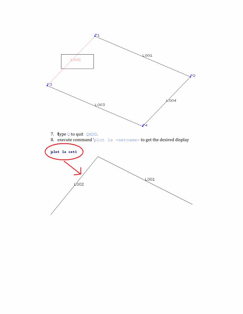
7. type Q to quit QADD.
8. execute command ‘plot la <setname> to get the desired display

Now moving on to the basic examples:
The intermediate images were obtained by plot and plus command.
EXAMPLE 1, DISC
CODES:
Create the required points:
pnt py 0.00000 1.00000 0.00000 pnt p0 0.00000 0.00000 0.00000 pnt p001 0.70711 0.00000 -0.70711 pnt p003 0.00000 0.00000 -1.00000 pnt p005 -0.70711 0.00000 -0.70711 pnt p006 -1.00000 0.00000 0.00000 pnt p009 -0.70711 0.00000 0.70711 pnt p00A 0.00000 0.00000 1.00000 pnt p00G 0.70711 0.00000 0.70711 pnt p00I 1.00000 0.00000 0.00000
Create the required lines: line l001 p00I p001 p0 4 line l002 p001 p003 p0 4 line l003 p003 p0 8 line l004 p0 p00I 8 line l005 p003 p005 p0 4 line l006 p005 p006 p0 4 line l007 p006 p0 8 line l009 p006 p009 p0 4 line l00A p009 p00A p0 4

line l00C p00A p0 8 line l00G p00A p00G p0 4 line l00I p00G p00I p0 4
Create the required surfaces:
gsur a001 + BlEND - l003 - l002 - l001 - l004 gsur a002 + BlEND - l007 - l006 - l005 + l003 gsur a003 + BlEND - l00C - l00A - l009 + l007 gsur a004 + BlEND + l004 - l00I - l00G + l00C

Create Elements and Mesh them ElTY all QU4 MESH all Left click-> left pane-> viewing->toggle model edge Plot ea all NOTE: The final image can be obtained by using viewing menu option

EXAMPLE 2: CYLINDER pnt p0 -0.00000 -0.00000 0.00000 pnt py -0.00000 1.00000 0.00000 pnt p1 1.00000 -0.00000 0.00000 pnt p001 1.00000 1.00000 0.00000 pnt p002 -0.00000 -0.00000 -1.00000 pnt p003 -0.00000 1.00000 -1.00000 pnt p006 -1.00000 -0.00000 0.00000 pnt p007 -1.00000 1.00000 0.00000 pnt p00A 0.00000 -0.00000 1.00000 pnt p00C 0.00000 1.00000 1.00000 line l001 p1 p001 2 line l002 p002 p003 2 line l003 p1 p002 p0 8 line l004 p001 p003 py 8 line l005 p006 p007 2 line l006 p002 p006 p0 8 line l007 p003 p007 py 8 line l008 p00A p00C 2 line l009 p006 p00A p0 8 line l00A p007 p00C py 8 line l00I p00A p1 p0 8 line l00J p00C p001 py 8
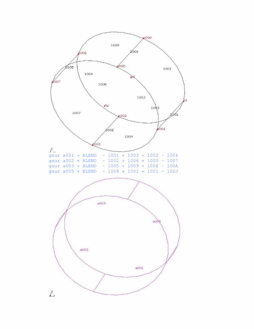
gsur a001 + BLEND - l001 + l003 + l002 - l004 gsur a002 + BLEND - l002 + l006 + l005 - l007 gsur a003 + BLEND - l005 + l009 + l008 - l00A gsur a005 + BLEND - l008 + l00I + l001 - l00J

ELTY all qu4 mesh all Left click-> left pane-> viewing->toggle model edg e plot ea all
NOTE: The final image can be obtained by using viewing menu option
EXAMPLE 3: SPHERE pnt py -0.00000 1.00000 -0.00000 pnt p1 1.00000 -0.00000 -0.00000 pnt p001 0.70711 -0.00000 -0.70711 pnt p003 -0.00000 -0.00000 -1.00000 pnt p006 0.70711 0.50000 -0.50000 pnt p008 -0.00000 0.70711 -0.70711 pnt p00C 0.70711 -0.00000 -0.00000 pnt p00K 0.70711 0.70711 -0.00000 pnt p00l -0.00000 -0.00000 -0.00000 pnt p00N -0.00000 1.00000 -0.00000 line l001 p1 p001 p00l 8

line l002 p001 p003 p00l 8 line l003 p1 p006 p00l 8 line l004 p006 p008 p00l 8 line l006 p001 p006 p00C 8 line l008 p003 p008 p00l 8 line l00A p1 p00K p00l 8 line l00C p00K p00N p00l 8 line l00G p006 p00K p00C 8 line l00J p008 p00N p00l 8
gsur A005 + blend - l003 + l001 + l006 gsur A002 + blend - l002 + l006 + l004 - l008 gsur A006 + blend + l003 + l00G - l00A gsur A004 + blend - l004 + l00G + l00C - l00J elty all qu4 mesh all Left click-> left pane-> viewing->toggle model edge plot ea all
NOTE: The final image can be obtained by using viewing menu option

EXAMPLE 4: SPHERE VOLUME
pnt py 0.00000 1.00000 0.00000 pnt p1 1.00000 0.00000 0.00000 pnt p006 0.70711 0.50000 -0.50000

pnt p008 0.00000 0.70711 -0.70711 pnt p00C 0.70711 0.00000 0.00000 pnt p00K 0.70711 0.70711 0.00000 pnt p00L 0.00000 0.00000 0.00000 pnt p00N 0.00000 1.00000 0.00000 line l001 p1 p00L 8 line l002 p00L p008 8 line l003 p1 p006 p00L 8 line l004 p006 p008 p00L 8 line l005 p00L p00N 8 line l00A p1 p00K p00L 8 line l00C p00K p00N p00L 8 line l00G p006 p00K p00C 8 line l00J p008 p00N p00L 8 gsur a001 + blend - l003 + l001 + l002 - l004 gsur a002 + blend - l005 - l001 + l00A + l00C gsur a006 + blend + l003 + l00G - l00A gsur a004 + blend - l004 + l00G + l00C - l00J gsur a003 + blend + l002 + l00J - l005 gbod B001 NORM + a006 - a003 - a004 + a002 + a001 ELTY all HE20 mesh all Left click-> left pane-> viewing->toggle model edge plot ea all


Reference:
[1] Calculix help file [2] http://www.dhondt.de/tutorial.txt


![Introduction to Wikimedia Commons [[User:MB-one]] Matti ... · Introduction to Wikimedia Commons Introduction What is Wikimedia Commons? “Wikimedia Commons is a database of content](https://img.pdfslide.net/doc/110x75/5fff7ce042830266fa4b39f8/introduction-to-wikimedia-commons-usermb-one-matti-introduction-to-wikimedia.jpg)