Nowcasting and Forecasting GDP in Emerging Markets Using Global Financialand Macroeconomic Diffusion Indexes∗

Oguzhan Cepni1, I. Ethem Guney1, and Norman R. Swanson2

1Central Bank of the Republic of Turkey and 2Rutgers University

March 2018

Abstract

In this paper, we contribute to the nascent literature on nowcasting and forecasting GDP in emerging market economies using

big data methods. This is done by analyzing the usefulness of various dimension reduction, machine learning and shrinkage

methods including sparse principal component analysis (SPCA), the elastic net, the least absolute shrinkage operator, and least

angle regression when constructing predictions using latent global macroeconomic and financial factors (diffusion indexes) in a

dynamic factor model (DFM). We also utilize a judgmental dimension reduction method called the Bloomberg Relevance Index

(BBG), which is an index that assigns a measure of importance to each variable in a dataset depending on the variable’s usage by

market participants. In our empirical analysis, we show that DFMs, when specified using dimension reduction methods (particularly

BBG and SPCA), yield superior predictions, relative to benchmark linear econometric or simple DFMs. Moreover, global financial

and macroeconomic (business cycle) diffusion indexes constructed using targeted predictors are found to be important in four of the

five emerging market economies (including Brazil, Mexico, South Africa, and Turkey) that we study. These findings point to the

importance of spillover effects across emerging market economies, and underscore the importance of parsimoniously characterizing

such linkages when utilizing high dimensional global datasets.

Keywords: Diffusion index, Dimension reduction methods, Emerging markets, Factor model, Forecasting,

Variable selection.

JEL Classification: C53, G17.

∗ Oguzhan Cepni (Oguzhan.Cepni@tcmb.gov.tr) and I. Ethem Guney (Ethem.Guney@tcmb.gov.tr), Central Bank of the Republic of Turkey,

Anafartalar Mah. Istiklal Cad. No:10 06050 Ulus, Altndag, Ankara, Turkey. Norman R. Swanson (nswanson@econ.rutgers.edu), Department of

Economics, 75 Hamilton Street, New Brunswick, NJ, 08901 USA. The authors wish to thank Hyun Hak Kim, Mingmian Cheng, Eric Ghysels,

Massimiliano Marcellino, Christian Schumacher, and Xiye Yang for useful discussions.

1. Introduction

Unlike financial variables which are collected at a relatively higher frequency and published in a timely

manner, initial estimates of GDP growth are often released many weeks after the reference quarter.1 Due

to this lack of timely information, government institutions, such as central banks, are forced to conduct

policy activity without complete knowledge of the current state of the economy. However, central bankers

do have timely information on variables that are released at higher frequencies than GDP, including data

on asset prices and many monthly macroeconomic and financial indicators. This has led to the flourishing

nascent literature on nowcasting using high dimensional datasets, which involves predicting the current

state of the economy before official figures are released. The key question that we attempt to answer in this

paper is whether it is possible to produce useful early signals of the current state of the economy, before

official figures are released. A practical issue that may hamper our efforts in this regard is the fact that many

datasets have missing data at the beginning of the sample, particularly in the case of the emerging market

economies that we examine. Thus, the usefulness of so-called big data is not a foregone conclusion. For

further discussion of nowcasting using big data, see Banbura et al. (2013), Bragoli et al. (2014), Forni and

Marcellino (2014), Hindrayanto et al. (2016), Modugno et al. (2016), Caruso (2017), Dalhaus et al. (2017),

Luciani et al. (2017), and the references cited therein.

Given the rich variety of high dimensional datasets that nowcasters now use, it is not surprising that

big data methods now play an important role in macroeconomic prediction. Indeed dimension reduction,

shrinkage and machine learning methods are utilized in various of the papers mentioned above. In this

paper, our objective is to also add to this literature by asking whether such methods are useful when study-

ing emerging market (EM) economies, including Brazil, Indonesia, Mexico, South Africa, and Turkey. We

start by analyzing the usefulness of various dimension reduction, machine learning and shrinkage meth-

ods. These so-called dimension reduction methods are used for constructing targeted sets of predictors, and

include: sparse principal component analysis (SPCA), the elastic net (ENET), the least absolute shrink-

age operator (LASSO), and least angle regression (LARS). For further discussion of dimension reduction

methods and prediction, see Boivin and Ng (2006), Schumacher (2007), Bai and Ng (2008), Banbura and

Runstler (2011), Kim and Swanson (2014, 2018), Bulligan et al. (2015), and the references cited therein.2

1The reference quarter is the calendar date to which the data pertains.2Bai and Ng (2002, 2006) and Doz et al. (2011, 2012) prove that diffusion indexes are consistent for large N and T , where N

denotes the number of variables, and T is the sample size, in a variety of factor modeling frameworks. Therefore, the common

1

It should be noted that we focus on the prediction of GDP growth for two main reasons. First, initial

quarterly GDP growth releases are subject to substantial differences in publication lags for developed and

emerging market economies. For example, while the first estimate of GDP is available in Euro area and

the U.S. three and four weeks after the quarter ends, initial GDP for Brazil and Turkey is not released until

10 and 12 weeks after the quarter ends, respectively. As GDP plays a central role in guiding economic

decision-making and policy analysis, the construction of timely short-term nowcasts of GDP is quite crucial

in the decision-making process of EM central banks. Second, emerging market economies where data are

often scant and unreliable presents additional challenges. When the quality of data is low (compared with

that available in developed market economies), a careful selection of predictive indicators is crucial when

constructing predictions. In these senses, it remains to be seen whether results concerning the usefulness

of dimension reduction methods and diffusion indexes found in the literature (e.g. see Kim and Swanson

(2014, 2018) and G. Bulligan et al. (2015)), carry over to the case of EM countries.

Summarizing, our approach in this paper is to utilize the dynamic factor modeling (DFM) framework

introduced by Giannone et al. (2008) in order to construct monthly predictions of quarterly GDP growth,

using a high dimensional global dataset. More specifically, predictions are constructed using either the entire

high dimensional dataset, including all variables for a country (or for a group of countries) or including

targeted predictors, where targeting is carried out using the SPCA, ENET, LASSO, LARS, and BBG method

discussed above. Our objective is thus to examine the relevance of two alternative types of diffusion indexes.

One variety utilizes only country specific data, both targeted and un-targeted; and one variety utilizes our

entire global dataset, both targeted and un-targeted. This approach builds on earlier work by Schumacher

(2010), Eickmeier and Ng (2011), Forni and Marcellino (2014), Caruso (2017), and by considering the

usefulness of global high dimensional datasets for predicting growth in emerging market economies.

Our empirical findings can be summarized as follows. First, there is a substantial reduction in mean

square forecast errors (MSFEs) as more data related to the current quarter become available, when backcast-

view among practitioners was previously that the dataset with the largest number of the indicators should be used to forecast

macroeconomic variables, since it might be argued that leaving out variables might result in a loss of potentially useful information

about the state of the economy. Also, the use of many variables reflects a central bank‘s motivation to show that it is taking all

potentially relevant information into account (see Bernanke and Boivin (2003)). However, a recent branch of the literature questions

the usefulness of “too much information” in factor model forecasting. For example, Boivin and Ng (2006) show that a small set of

indicators, when chosen appropriately, improves macroeconomic forecasts. They select their indicators using the LASSO. Stock

and Watson (2012) and Kim and Swanson (2014) discuss the use of other dimension reduction methods in this context, and also

find that forecasts can be improved using targeted predictors.

2

ing, nowcasting, and forecasting. Thus, the DFM methodology adequately incorporates new information,

even for EM countries with data quality issues.

Second, predictions based on dimension reduction, machine learning and shrinkage work for EM coun-

tries. In particular, benchmark time series models (e.g. autoregressive models), as well as DFMs that do

not utilize dimension reduction yield inferior predictions in almost all of the prediction experiments that we

ran. Interestingly, the BBG method ranks as the best dimension reduction method, with SPCA coming in

second. Together, these targeted predictor selection methods yield MSFE-“best” models around 80% of the

time. More specifically, when comparing results across different prediction horizons and across countries,

SPCA yields MSFE-best predictions in 14 of 50 cases. (BBG “wins” in 23 out of 50 cases). Thus, while

not a crowd source type of dimension reduction like BBG, the SPCA method clearly performs well, particu-

larly given that it is a purely data-driven statistical learning method. Additionally, it is worth noting that our

non-BBG dimension reduction methods, which are all purely statistical, perform their best for nowcasts and

backcasts. Indeed, they are MSFE-best in 15 of 20 cases when considering only nowcasts and backcasts.

Thus, the expert judgment associated with using the BBG index is less useful for near-term forecasting,

relative to SPCA, ENET, LASSO, and LARS.

Finally, models that include our global EM diffusion indexes are usually MSFE-best, for all forecast

horizons, as well as across all dimension reduction methods. For example, global EM diffusion indexes

are included in the MSFE-best model for every prediction horizon, and across every dimension reduction

method, in the case of Brazil. For Mexico, South Africa, and Turkey, the picture is also quite clear. Global

EM diffusion indexes yield substantial predictive gains, as “Local” and “Local-AR” are the MSFE-best

models in only 13 of 30 cases, across all dimension reduction methods for these countries. Interestingly,

the same cannot be said for Indonesia, as “Local” and “Local-AR” are the MSFE-best models in 6 of 10

cases, across all dimension reduction methods. In summary, we have very strong evidence that global EM

diffusion indexes have useful predictive content, suggesting that linkages across EM economies can be

modeled using diffusion indexes, and are useful for predicting GDP growth in emerging market economies.

The rest of the paper is structured as follows. In Section 2, we outline the empirical methodology used

in the sequel. This includes discussions of dynamic factor models, dimension reduction methods, and the

setup used in our prediction experiments. In Section 3, we describe the dataset utilized in our experiments.

Section 4 contains a discussion of our empirical findings. Finally, concluding remarks are collected in

Section 5.

3

2. Empirical Methodology

2.1. Dynamic Factor Model

The starting point of our analysis is the widely used dynamic factor model (DFM) of Giannone et al.

(2008). As is typical in such models, individual variables are represented as the sum of components that are

common to all variables in the economy (i.e., the factors) and an orthogonal idiosyncratic component. As

we shall see later, we also allow for an autoregressive component in our final prediction models.

Formally, the DFM can be written as a system of equations: a measurement equation (i.e., Eq. (1)) that

links the observed variables to the unobserved common factor to be estimated, and transition equations (i.e.,

Eq. (2) and Eq. (3)) that describe the dynamics of the common factor and the residuals of the measurement

equation. Once Eqs. (1)-(3) are written in state space form, we utilize the Kalman filter and smoother in

order to extract the common factors and generate projections for all of the variables in the model.

In the sequel, we consider a panel of observable economic variables Xi,t where i indicates the cross-

section unit, i = 1, ...,N and t denotes the monthly time index, t = 1, ...,T . Each variable in the dataset can

be decomposed into a common component and an idiosyncratic component, where the common components

capture comovements in the data, and are driven by a small number of shocks. Summarizing, the dynamic

factor model can be written as:

Xt = ΛFt + ξt, ξt ∼ N(0,Σe), (1)

Ft =

p∑i=1

ΨiFt−i + ut, ut ∼ N(0,Q), (2)

and

ξt = ρξt−1 + εt εt ∼ N(0, σ2), (3)

where Ft is an r× 1 vector of unobserved common factors with zero mean and unit variance, that reflect

“most” of the co-movements in the variables, Λ is a corresponding N × r factor loading matrix, and the

idiosyncratic disturbances, ξt, are uncorrelated with Ft at all leads and lags, and have a diagonal covariance

matrix, Σe. It is assumed that the common factors, Ft, follow a stationary VAR(p) process driven by the

common shocks, ut ∼ N(0,Q), and that the Ψi are r × r matrices of autoregressive coefficients. Also, the

common shocks, ut, and the idiosyncratic shocks, εt, are assumed to be serially independent and independent

of each other over time, while weak cross and serial correlation in the idiosyncratic shocks are allowed.

4

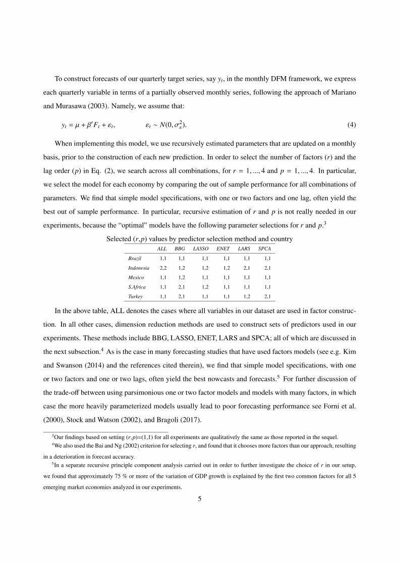
To construct forecasts of our quarterly target series, say yt, in the monthly DFM framework, we express

each quarterly variable in terms of a partially observed monthly series, following the approach of Mariano

and Murasawa (2003). Namely, we assume that:

yt = µ + β′Ft + εt, εt ∼ N(0, σ2ε). (4)

When implementing this model, we use recursively estimated parameters that are updated on a monthly

basis, prior to the construction of each new prediction. In order to select the number of factors (r) and the

lag order (p) in Eq. (2), we search across all combinations, for r = 1, ..., 4 and p = 1, ..., 4. In particular,

we select the model for each economy by comparing the out of sample performance for all combinations of

parameters. We find that simple model specifications, with one or two factors and one lag, often yield the

best out of sample performance. In particular, recursive estimation of r and p is not really needed in our

experiments, because the “optimal” models have the following parameter selections for r and p.3

Selected (r,p) values by predictor selection method and countryALL BBG LASSO ENET LARS SPCA

Brazil 1,1 1,1 1,1 1,1 1,1 1,1

Indonesia 2,2 1,2 1,2 1,2 2,1 2,1

Mexico 1,1 1,2 1,1 1,1 1,1 1,1

S.Africa 1,1 2,1 1,2 1,1 1,1 1,1

Turkey 1,1 2,1 1,1 1,1 1,2 2,1

In the above table, ALL denotes the cases where all variables in our dataset are used in factor construc-

tion. In all other cases, dimension reduction methods are used to construct sets of predictors used in our

experiments. These methods include BBG, LASSO, ENET, LARS and SPCA; all of which are discussed in

the next subsection.4 As is the case in many forecasting studies that have used factors models (see e.g. Kim

and Swanson (2014) and the references cited therein), we find that simple model specifications, with one

or two factors and one or two lags, often yield the best nowcasts and forecasts.5 For further discussion of

the trade-off between using parsimonious one or two factor models and models with many factors, in which

case the more heavily parameterized models usually lead to poor forecasting performance see Forni et al.

(2000), Stock and Watson (2002), and Bragoli (2017).

3Our findings based on setting (r,p)=(1,1) for all experiments are qualitatively the same as those reported in the sequel.4We also used the Bai and Ng (2002) criterion for selecting r, and found that it chooses more factors than our approach, resulting

in a deterioration in forecast accuracy.5In a separate recursive principle component analysis carried out in order to further investigate the choice of r in our setup,

we found that approximately 75 % or more of the variation of GDP growth is explained by the first two common factors for all 5

emerging market economies analyzed in our experiments.

5

2.2. Dimension reduction methods for selecting targeted predictors

Since our dataset is characterized by a large number variables (see Section 3), it is important to select

appropriate “targeted” predictors prior to estimating factor models. The reason why this is the case is that

model and parameter uncertainty can adversely impact the marginal predictive content of factors that are

constructed using finite samples of data. Moreover, directly using least squares or other standard estimators

is not feasible in contexts that considered in this paper, since the number of regressors that we consider is

greater than the number of observations. These issues are discussed at length in Bai and Ng (2008), Kuzin

et al. (2011,2013), Stock and Watson (2012), Kim and Swanson (2014, 2018), and many others. For this

reason, we utilize variable selection or dimension reduction methods in order to pre-select predictors prior

to the construction of factors. Many of the shrinkage and machine learning methods that are examined

by the above authors in this context can be interpreted as penalized estimation problems. For example,

Kim and Swanson (2018) implement a number of interesting variable selection and shrinkage methods,

including bagging, boosting, least angle regression, and the nonnegative garrote, and find strong evidence

of the usefulness of dimension reduction techniques in the context of out-of-sample forecasting of 11 U.S.

macroeconomic variables. Bai and Ng (2008) implement the least absolute shrinkage selection operator

and the elastic net in order to construct targeted predictor datasets, and find improvements at all forecast

horizons when estimating factors using fewer informative predictors. Also, Bulligan et al. (2015) show that

soft thresholding methods can be used successfully to reduce the size of large panels of economic data.

In this paper, we implement a variety of variable selection and shrinkage methods in order to obtain

targeted predictors for use in our factor model, including:

• Least absolute shrinkage selection operator (LASSO)

• Elastic net estimator (ENET)

• Least angle regressions (LARS)

• Sparse Principal Component Analysis (SPCA)

Namely, we consider a panel of observable economic variables Xi,t, where i indicates the cross-section

unit, i = 1, ...,N, and t denotes the time index, i = 1, ...,T , as discussed above. Following the notation of

Hastie et al. (2009), we consider the problem of selecting a subset of X, where X is a T × N matrix to be

used for forecasting scalar annualized GDP growth, say Y , for i = 1, ...,T .

6

2.2.1. Sparse principal component analysis

Sparse principal component analysis (SPCA), introduced by Zou et al. (2006), is a variant of principal

component analysis (PCA). PCA yields orthogonal latent factors that are maximally correlated with all

variables in X. One potential disadvantage of this method is that each principal component is a linear

weighted combination of all variables in the original dataset, with no weights equal to zero. Thus, all

variables are included in all factors. SPCA, which can be interpreted as double-shrinkage using the elastic

net, combines L1 and L2 penalty functions (in a penalized regression problem) in order to “shrink” weights

from PCA factors to zero. In this way, factors constructed using SPCA contain non-zero weights only on

selected (or targeted) predictors. Setting various factor loading coefficients equal to zero in this way has the

potential to reduce “noisiness” of factors, and also aid in the economic interpretation of factors.

The SPCA problem can be formulated as the following maximization problem:

maximizeX

vT (XT X)v,

subject toN∑

j=1

|v j| 6 ψ,

vT v = 1.

where X is the data matrix, the v are principal components (possibly with zero loadings), and ψ is a some

tuning parameter. Optimization in this context is not trivial, and various algorithms are suggested in the lit-

erature that based on a convex semidefinite programming, generalized power methods, greedy search meth-

ods, and exact methods using branch-bound techniques. Following the Naikal et al. (2011), we implement

the augmented Lagrange multiplier method for extracting the sparse principal components. In particular,

we select first factor (i.e., maximal correlation factor), and our targeted predictors are those variables with

non-zero factor loading coefficients in said factor.

2.2.2. Least absolute shrinkage operator (LASSO)

We also implement the LASSO, which was introduced by Tibshirani (1996), and can be written as

a penalized regression problem, just like the well know ridge estimator, for example. However, LASSO

imposes an `1-norm penalty on the regression coefficients, rather than an `2-norm penalty, as is the case

with the well known ridge estimator. This penalty results in (possible) shrinkage of coefficients (called

7

βlasso below) to zero. The LASSO estimator is given below.

βlasso =minβ‖Y − Xβ‖2 + λ

N∑j=1

|β j|, (5)

where λ is a tuning parameter that controls the strength of the `1-norm penalty. Since the objective function

in the LASSO is not differentiable, numerical optimization must be used when constructing βlasso. For

example, an efficient iterative algorithm called the “shooting algorithm” is proposed in Fu (1998). One of

the limitations of the LASSO approach is that the number of selected variables is bounded by the sample

size. For example, if N > T, the LASSO yields at most N non-zero coefficients (see Swanson (2016) for

further discussion). The variables associated with these non-zero coefficients constitute our set of targeted

predictors when using the LASSO. We utilize the algorithm of Fu (1998) in our experiments.

2.2.3. Elastic Net (ENET)

The LASSO is naturally adapted to cases where there are many zero coefficients in the “true” model.

However, in the presence of highly correlated predictors, Tibshirani (1996) shows that the predictive per-

formance of the LASSO is sometimes worse than the forecasts that are constructed using ridge regression.

Zou and Hastie (2005) address this issue by proposing a hybrid form of the LASSO and ridge estimators,

called the elastic net (ENET) estimator. The ENET estimator is defined as follows:

βEN =minβ‖Y − Xβ‖2 + λ1

N∑j=1

|β j| + λ2

N∑j=1

β j2, (6)

where there are now two tuning parameters, λ1 and λ2 controlling the two penalty functions. The EN

estimator also results in possible shrinkage of coefficients to zero, although in cases where N > T, the EN

can yield more than N non-zero coefficients.

2.2.4. Least Angle Regressions (LARS)

Least angle regression was proposed by Efron et al. (2004). The algorithm is similar to forward step-

wise regression, but instead of including variables at each step, the algorithm proceeds equi-angularly in

directions that are chosen to impose equal correlations with each of the variables currently in the model.

Moreover, (LARS) can easily be reformulated to obtain solutions for other estimators, like the LASSO and

EN. It allows for the ranking of different predictors according to their predictive content, which is not the

case when using hard thresholding methods. Thus, sparsity can be obtained by selecting only the highest

ranked variables for model estimation. In this paper, we follow the approach of Efron et al. (2004) when

implementing LARS.

8

2.2.5. Bloomberg relevance index (BBG) for selecting targeted predictors

In addition to above techniques, we investigate selected targeted predictors based on observing which

economic variables are monitored by the markets. This type of expert judgement method is developed by

Banbura et al. (2013), and has been used by Luciani and Ricci (2014), Bragoli et al. (2014) and Luciani

et al. (2017). The main assumption of this approach is that market participants monitor macroeconomic

data and use them to form their expectations about the state of the economy in order to allocate their

investments. In this context, the Bloomberg reports “relevance index”, which we call the BBG index, for

numerous economic variable that is closely followed by market participants. We select the variables based

on this index. As Bloomberg only reports current values for this index, all of our BBG targeted predictors

are based on Bloomberg information available at the time that our dataset was pulled (i.e., January 2018).

In order to maintain comparability across all of different predictor selection methods in our experiments, all

other methods were applied using the same dataset as that available to users of Bloomberg in January 2018.

More specifically, when Bloomberg users put an “alert” on the release date of a variable in the Bloomberg

database, then the Relevance index for that variable increases. For simplicity, we select all variables that

have a BBG index bigger than zero. For our five countries, including Turkey, Indonesia, Mexico, South

Africa, and Brazil the BBG index selects 20, 16, 22, 23, and 28 variables for Turkey, Indonesia, Mexico,

S.Africa and Brazil, respectively.6

2.2.6. Selected predictors for five emerging market economies

In order to provide insight into the predictors that are selected using the five above methods, the key

variables (i.e., those that are chosen for at least 4 of the 5 above methods) are listed Table 1.7 Some

interesting conclusions can be drawn in terms of cross-country differences and similarities when comparing

the variables for each of our five countries.

For Turkey, note that many variables are related to industrial production and its subcomponents, all

of which play an important leading role in driving cyclical fluctuations in GDP growth. Also, Turkish

economy is driven to a great degree by domestic demand (i.e., consumption expenditures), and when the

economy is in an expansion phase, imports tend to increase markedly. It is thus not surprising that imports,

6Targeted predictors used in our experiments are selected only once, based on analysis of our entire dataset. This is an approxi-

mation of the approach that a central bank might take, for example, of selecting a new set of predictors prior to the construction of

each prediction, and is predicated on the lack of data availability in our sample period.7The full list of the selected predictors, by method, is available upon request from the authors.

9

which are good predictors of consumption expenditures, are in the set of selected predictors. Finally, it is

worth noting that confidence indexes are important predictors for Turkey, suggesting that these indexes are

accurate measures of consumer and producer sentiment.

For Mexico, selected predictors are mainly export measures. This is not altogether surprising, given that

Mexico relies heavily on trade, and is the most important trade partner of the USA. Indeed, non-petroleum

exports to the US comprises nearly 83% of their total non-petroleum exports. Total vehicle production is

another important indicator. The automobile sector in Mexico differs from that in other emerging mar-

ket countries because it produces technologically complex components, while other countries function as

“assembly” manufacturers. Finally, variables related to labor force statistics are important for Mexico.

Brazil's economy also relies heavily on exports, and so it is not surprising that the predictors selected

include various trade related variables. Also, although commodities-related sectors play an important role in

Brazil, manufacturing sectors also play a significant role in the economy. Hence, the labor force and working

hours variables related to the manufacturing industry are also relevant for GDP growth. Furthermore, three

retail sales indexes are key predictors, which is not surprising since the main driver of the GDP growth

is private consumption. Interestingly, two of these retail indexes are construction related, suggesting that

government efforts to revitalization through the implementation of urbanization programs is an important

driver of growth in Brazil.

Similar pattern emerges when viewing variables selected for Indonesia. Namely, exports and imports

matter, as do a number of retail sales indexes. On the other hand, predictors for Indonesia include not only

real variables but also financial variables, such as external debt and loans. This is not surprising for an

emerging market economy, since capital loan growth is a key indicator of new investment, which is in turn

a predictor for GDP growth.

For South Africa, we also observe that financial variables are important. One reason for this may be that

levels of domestic savings are inadequate, resulting in heavy reliance on capital in-flows in order to spur

economic growth.

2.3. Prediction experiments

In order to evaluate the forecasting performance of the above dynamic factor model, we carry out a series

of recursive pseudo out-of-sample forecasting experiments, where monthly forecasts for the five emerging

market economy GDP growth rates are constructed, for the prediction period July 2008 - September 2017.

Additionally, the experiments are repeated using the various different dimension reduction methods dis-

10

cussed above. For each reference quarter (recall that GDP is measured quarterly), we produce a sequence

of ten monthly predictions, starting with a forecast based on information available in the first month of the

two previous quarters and ending with a forecast based on information available in the first of month of

the subsequent quarter before GDP is actually released. Thus, we construct three monthly forecasts (for

quarterly forecast horizon, h = 2), three monthly forecasts (for quarterly forecast horizon, h = 1), three

monthly nowcasts (for quarterly forecast horizon, h = 0), and one monthly backcast (for quarterly forecast

horizon, h = −1).

We carry out two varieties of experiment. In our first set of experiments, we directly investigate the fore-

casting performance of DFM predictions based on pre-selection of predictors from large panels of macroe-

conomic data (see Section 3 for a discussion of the data used). Namely, for each country, the following

five dimension reduction methods are utilized in order to select predictors for inclusion in the DFM model:

BBG, LASSO, ENET, LARS, and SPCA. Two benchmark models are also utilized to construct predictions,

including an autoregressive (AR) model, with lags selected via use of the Schwarz information criterion

(SIC) and a version of our DFM model, called “ALL” in Table 2, where factors are extracted using all of

the domestic variables for a given country. Comparison of our targeted predictor results with AR and ALL

allows us to assess predictive accuracy relative to a standard straw-man model used widely in the literature

(i..e, the AR model), and with a factor model where predictors are not targeted (i.e., the ALL model).

In our second set of experiments, we combine the targeted predictors used in our first set of experiments

across all five countries. This resulting set of “Global” targeted predictors is then partitioned into three sets

of variables: “Global” (includes all variables), “Macroeconomic” (includes only macroeconomic variables)

and “Financial” (includes on financial variables). These subsets of variables are individually used to specify

new factors that are “added” to our DFM model. In particular, three new diffusion indexes (i.e., factors) are

constructed for each economy. These new diffusion indexes are called the EM Global factor (constructed

using “Global” variables), the EM Macro factor (constructed using “Macroeconomic” variables), and the

EM Financial factor (constructed using “Financial” variables).8 The new factors are then included in the

following four specifications, in which Specification 1 is simply the model in Eq. (4), and Specifications

2-4 are extensions that include our new diffusion indexes.

8Note that the cross country diffusion indexes (i.e., factors) that we extract for each country do not include local variables from

the corresponding country for which the new factors are being constructed.

11

• Specification 1: Local Diffusion Index model

yt+h = µ + β′FLocalt + εt+h

• Specification 2: EM Global factor model

yt+h = µ + β′FLocalt + ϑ′FEMGlobal

t + εt+h

• Specification 3: EM Macro factor model

yt+h = µ + β′FLocalt + θ′FEMMacro

t + εt+h

• Specification 4: EM Macro-Financial factor model

yt+h = µ + β′FLocalt + θ′FEMMacro

t + δ′FEMFinancialt + εt+h

Finally, four additional variants of Specifications 1-4 that include lags of yt, with lags selected via use

of the SIC, are analyzed in our experiments. Moreover, as done in our first set of experiments, we also

construct predictions using a purely autoregressive model, called AR above.

We assess the precision of the different sequences of forecasts constructed in the above experiments

using the mean square forecast error (MSFE), which is measured as the average of the squared differences

between predicted and actual GDP growth rates. In order to assess the statistical significance of differences

in MSFE across models and methods, we also conduct predictive accuracy tests using the Diebold-Mariano

(DM: 1995) test, which is implemented using quadratic loss, and which has a null hypothesis that the two

models being compared have equal predictive accuracy. For a complete discussion of inference based on

the DM test in cases where models are nested and in cases where parameter estimation error is accounted

for in the limit distribution of the test statistic, refer to McCracken (2000) and Corradi and Swanson (2006,

2007).

3. Data

The dataset used in this paper includes a relatively large set of economic indicators consisting of 103,

103, 117, 110 and 88 economic series for Turkey, Brazil, Mexico, South Africa, and Indonesia respectively.

These series are selected to represent broad categories of economic indicators. Examples of the variables

include supply-side indicators, such as industrial production indexes, and demand-side indicators such as

electricity consumption. Various survey variables are also included in the dataset, such as the Markit PMI

survey, which is one of the most watched business cycle indicators currently available. Given the sensitivity

of emerging market economies to external conditions, we also include value and volume indexes of exports

12

and imports, as well as real effective exchange rates. All data were downloaded from Bloomberg, and a

complete list of variables is available at http://econweb.rutgers.edu/nswanson/papers.htm.

More specifically, the dataset covers the period January 2005 - September 2017 and can be divided into

six categories: Housing and Order Variables: House price index, completed buildings recorded and new

orders. Labor Market Variables: Employment and unemployment. Prices: Producers prices and consumer

prices. Financial Variables: interest rates, exchange rates, and stock prices. Money, Credit and Quantity

Aggregates: money supply, mortgage loans, time and sight deposits. Real Economics Activity: PMI survey,

industrial production, retail sales and capacity utilization. All series are made stationary by differencing

or log-differencing, as needed. With regard to the timing of data releases, note that survey variables and

nominal indicators are usually released during the reference month (i.e., calendar date of the observation),

while real and labor variables are released with a publication lags of 1-3 months.

Of final note is that the data that we examine are not real-time, in the sense that we do not analyze a

sequence of revisions for each calendar dated observation. Rather, we assume that all data are final revisions.

In this sense, our experiments are only pseudo real-time in nature. Construction of real-time datasets for the

countries in our analysis, which will enable us to carry out truly real-time prediction experiments, is left to

future research.

4. Empirical Results

4.1. Mining big data using dimension reduction methods

Table 2 summarizes the results of our first set of prediction experiments, in which we compare the

five dimension reduction methods utilized in order to select targeted predictors prior to construction of

predictions using dynamic factor models. The table is vertically partitioned into five sets of results for our

five EM economies. Entries in the table are either MSFEs (for the AR(SIC) model listed in the first row of

entries for each country), or relative MSFEs (for all other rows under each country), where the numerator

in the relative MSFEs is the MSFE of the benchmark AR(SIC) model. In particular, entries are MSFEs

for various types of predictions. For each of two quarterly h-step ahead forecast horizons, (i.e., h = 1

and h = 2), MSFEs from three monthly forecasts (denoted as month “1”, “2” and “3” of the quarter in

the second row of entries in the table). Results are also reported for three monthly nowcasts (for quarterly

forecast horizon, h = 2), and for one monthly backcast (for quarterly forecast horizon, h = −1). For each

country, entries denoted in bold and subscripted with ”LB” (for “locally-best”) indicate the MSFE-“best”

13

models across all dimension reduction methods, for a given forecast horizon and country. A summary of

the“best” dimension reduction methods from this table is given in Table 8.

The results in Table 2 reveal various interesting insights.

First, there is a substantial reduction in MSFEs as more data related to the current quarter become

available, as is clearly evident by scanning the rows of the table from left to right as one moves from

forecasting (least information) to backcasting (most information). Thus, the DFM is incorporating new

information effectively (see Giannone et al., (2008) and Banbura and Runstler (2011) for further discussion).

Second, with a limited number of exceptions, the entries in Table 2 are less than unity, which indicates

that our predictions are quite accurate, relative to the benchmark model. Additionally, the magnitude of the

MSFEs is similar for most countries, except for Turkey, where errors are much larger due to higher GDP

growth volatility.

Third, recall that there are ten forecast horizons and five countries, so that we have a total of 50 speci-

fications for each dimension reduction method. Among the different methods, the BBG criterion performs

surprisingly well, as it attains the top rank in 23 out of 50 cases. This can be seen from Table 2 by noting

that the lowest MSFEs are denoted in bold. Indeed, the average MSFEs of BBG type predictions are 31%,

23%, 47%, 36%, and %34 lower than those associated with the AR model, for Brazil, Indonesia, Mexico,

South Africa, and Turkey, respectively. Of note is that Bloomberg collects forecasts from market analysts

to produce their own GDP growth forecasts (generally around two weeks before the release of new GDP

data). Their predictions are revised continually up to 24 hours before the release of actual data. This implies

that market analysts continually monitor all macroeconomic data to form expectations on current and future

GDP growth values, and this monitoring behavior is reflected in the BBG index that we use, since it is based

on user subscriptions to Bloomberg news alerts for specific data releases of variables deemed important. The

BBG index, thus, can be interpreted as a variety of big data based crowd sourcing information.

Fourth, SPCA also fares quite well, yielding MSFE-best predictions in 14 of 50 cases. While not a

crowd source type of dimension reduction like the BBG index, the SPCA method clearly performs well,

particularly given that it is a purely data-driven statistical learning method. Additionally, it is worth noting

that our non-BBG index methods, which are all purely statistical, perform their best for nowcasts and back-

casts. Indeed, they are MSFE-best in 15 of 20 cases when considering only nowcasts and backcasts. Thus,

the expert judgment associated with using the BBG index is not particularly useful for near-term forecast-

ing, relative to already existing methods of dimension reduction. However, when constructing predictions

14

for h=1 and h=2, using the BBG index yields superior predictions in 19 of 30 cases.

Fifth, Figure 1 plots actual GDP growth together with monthly nowcasts obtained from the use of the

BBG and SPCA selection methods. Examination of these plots indicates that DFM based on these dimen-

sion reduction methods tends to predict turning points relatively well, and outperforms the benchmark AR

models particularly well during volatile episodes. This suggests that the selection of relevant predictors

from a large datasets mitigates data noisiness that increases during periods of higher than normal volatility.

Why? Perhaps this is because correlations across broad spectra of variables increase during market down-

turns and volatile periods. This in turn magnifies the multicollinearity problem that characterizes the use of

dataset where N is very large. Indeed, the efficacy of asymptotic theory associated with the use of principal

components in time series contexts (see e.g. Bai and Ng (2002, 2006, 2008)) often relies on assumption that

cross-correlation between the errors in factor models is not too large.

Finally, our results validate the findings of Boivin and Ng (2006), where it is suggested that correlation

and data “noisiness” creates a situation where more data might not be desirable. Indeed, we find that models

utilizing expert judgment (BBG), as well as machine learning and shrinkage methods yield very accurate

forecasts when compared with factor models that do not use dimension reduction (see entries denoted by

ALL in Table 2), and when compared with benchmark autoregressive models.

4.2. Exploiting cross-country linkages when constructing diffusion indexes

The objective of our second set of experiments is to provide a comprehensive empirical characterization

of useful business cycle linkages between emerging markets using a dynamic factor model. In particular,

we address the following question: Does taking cross-country business cycle factors into account lead to

marginal gains in terms of predictive accuracy when analyzing emerging market economies? As discussed

in Section 2.3, we attempt to answer this question by estimating three additional factors: EM Global, EM

Macro and EM Financial; and by utilizing these new diffusion indexes in our predictive modeling. Recall

that the factors utilized in our first set of experiments were constructed using only local or “own-country”

variables. Our EM diffusion indexes utilize data that is pooled across all EM economies. Before discussing

the usefulness of these global common factors, it is of interest to investigate the correlation between the

GDP growth rates across our EM economies. The below chart reports the correlation coefficients between

growth rates of the five countries. These correlation coefficients range from 0.16 to 0.70, indicating that

GDP growth rates across countries are significantly correlated. While this is not surprising, it does indicate

that the global diffusion indexes that we are discussing in this section might indeed be useful for prediction.

15

GDP growth rate correlation coefficientsTurkey Brazil Indonesia S.Africa Mexico

Brazil 0.39 1 0.46 0.67 0.35

Indonesia 0.04 0.46 1 0.24 0.16

Mexico 0.70 0.35 0.16 0.54 1

S.Africa 0.44 0.67 0.24 1 0.54

Turkey 1 0.39 0.04 0.44 0.70

In order to provide insight regarding the evolution of global and country-specific factors, Figure 2 plots

GDP growth against estimated common factors. As shown, both local and global common factors track

GDP growth quite well, and they can be a good proxy for GDP dynamics in these countries during the

global financial crisis.

Tables 3-7 summarize the results of our second set of prediction experiments. As discussed above,

bold entries denote the forecasting models that are MSFE-best dimension reduction method. Thus, for

BBG, when h=2, and the month is “1”, the EM Macro-Financial-AR model is MSFE-best. This means that

our model that includes both global macroeconomic and global financial variables is superior to all other

models, when dimension reduction is carried out using the BBG index. Entries subscripted with ”GB”

denote the MSFE-best model for a given forecast horizon across all dimension reduction methods. Thus,

BBG is also the best dimension reduction method, across all 6 methods, including ALL, BBG, LASSO,

ENET, LARS, and SPCA, for h=2, when the month is “1”. A summary of such MSFE-best models across

dimension reduction methods for each forecast horizon is given in Table 9. An inspection of Tables 4-8

leads to a number of clearcut conclusions.

First, although there are a limited number of exceptions, most of the entries in Tables 3-7 are below one,

again indicating that dynamic factor model forecasts are more accurate than those constructed using our

benchmark AR(SIC) models. The plethora of rejections of the null hypothesis of equal predictive accuracy

when comparing our non-autoregressive type models with the AR(SIC) benchmark (note that there are many

entries in the tables that are superscripted with a * or **, indicating DM test rejection), is further evidence

of this finding. Additionally, we again see that our factor models generally yield more accurate predictions

as more information arrives, within each quarter.

Second, when comparing the “globally best” models across all forecast horizons, it is clear that the

MSFE-best models are generally those that utilize dimension reduction methods for selecting targeted pre-

dictors, and are not based on ALL or on the use of AR(SIC) models. This is further confirmation of our

above findings, as is the fact that BBG and SPCA win in 32 of 50 cases. Thus, data shrinkage and dimension

16

reduction methods are indeed useful.

Third, the models labeled “Local” and “Local-AR” in Tables 3-7 are not usually the MSFE-best mod-

els. Instead, models that include our global EM diffusion indexes are usually MSFE-best, for all forecast

horizons, as well as across all dimension reduction methods. For example, global EM diffusion indexes

are included in the MSFE-best model for every prediction horizon, and across every dimension reduction

method, in the case of Brazil. For Mexico, South Africa, and Turkey, the picture is also quite clear. Global

EM diffusion indexes yield substantial predictive gains, as “Local” and “Local-AR” are the MSFE-best

models in only 12 of 30 cases, across all dimension reduction methods for these countries. Interestingly,

the same cannot be said for Indonesia, as “Local” and “Local-AR” are the MSFE-best models in 6 of 10

cases, across all dimension reduction methods.9 Given these findings, it should come as no surprise that

GDP growth rates are contemporaneously correlated with all of the diffusion indexes analyzed in this paper.

Figure 3 plots correlation coefficients from simple regressions of GDP growth in each country against our

“Local” as well as our global EM diffusion indexes. Inspection of this figure indicates that local diffusion

indexes exhibit high correlation with GDP growth. However, correlation with global EM indexes is also sur-

prisingly high, supporting our finding that using both local and global indexes yields superior predictions

for most countries, regardless of the variety of dimension reduction that is utilized.

In summary, we have very strong evidence that global EM diffusion indexes have useful predictive

content, suggesting that linkages across EM economies can be modeled using diffusion indexes, and are

useful for predicting GDP growth in emerging market economies.

9Note the low correlations between Indonesian GDP growth rates and the growth rates for Brazil, Mexico, South Africa and

Turkey.

17

5. Conclusion

Dynamic factor models are widely used in the forecasting literature. However, relatively few of these

papers analyze the usefulness of dimension reduction, machine learning, and shrinkage methods for se-

lecting targeted predictors to include in factor models. In this paper, we compare the use of multiple such

methods for constructing “local” and “global” diffusion indexes, in the context of GDP growth prediction

in emerging market (EM) economies. We find that dimension reduction matters. In particular, a so-called

Bloomberg relevance index (BBG), which is related to crowd-sourcing coupled with expert opinion, as well

as sparse principal component analysis, are particularly useful for selecting targeted predictors when con-

structing diffusion indexes. We also find that global diffusion indexes, which capture “spillover” effects

among countries, are useful for nowcasting and forecasting EM GDP growth. In particular, exploiting the

informational content of business cycle diffusion indexes based on macroeconomic and financial variables

pooled across multiple economies leads to improved prediction of GDP growth, relative to the case where

only “own-economy” variables are used when constructing diffusion indexes.

This paper is meant as a starting point, as many questions remain unanswered. For example, it should

be of interest to collect the Bloomberg BBG index in real-time, and to assess the usefulness of the index for

prediction. Currently, the index is available only as a point estimate of variable relevance. Collecting time

series which measure the relevance of variables may yield further interesting insights into the usefulness

of crowd-sourcing big data methods. Additionally, our analysis focuses on emerging market economies. It

remains to assess how one might utilize linkages between developed and emerging markets when predicting

economic variables of EM economies.

18

References

Bai, J., and Ng, S. (2002). Determining the number of factors in approximate factor models. Econo-

metrica, 70, 191-221.

Bai, J. and Ng, S. (2006a). Confidence intervals for diffusion index forecasts and inference for factor-

augmented regressions. Econometrica, 74, 1133-1150.

Bai, J., and Ng, S. (2008). Forecasting economic time series using targeted predictors. Journal of

Econometrics, 146, 304-317.

Banbura, M., Giannone, D., Modugno, M., and Reichlin, L. (2013). Now-casting and the real-time data

flow. In G. Elliot and A. Timmermann, (eds.), Handbook of Economic Forecasting, Volume 2, Elsevier:

Amsterdam.

Banbura, M., and Runstler, G. (2011). A look into the factor model black box: publication lags and the

role of hard and soft data in forecasting GDP. International Journal of Forecasting, 27, 333-346.

Bernanke, B. S., and Boivin, J. (2003). Monetary policy in a data-rich environment. Journal of Monetary

Economics, 50, 525-546.

Boivin, J., and Ng, S. (2006). Are more data always better for factor analysis? Journal of Econometrics,

132, 169-194.

Bragoli, D., Metelli, L., and Modugno, M. (2014). The importance of updating: evidence from a

Brazilian nowcasting model. Board of Governors of Federal Reserve System, Working Paper No. 2014-94.

Bragoli, D. (2017). Now-casting the Japanese economy. International Journal of Forecasting, 33, 390-

402.

Bulligan, G., Marcellino, M., and Venditti, F. (2015). Forecasting economic activity with targeted

predictors. International Journal of Forecasting, 31, 188-206.

Caruso, A. (2017). Nowcasting with the help of foreign indicators: the case of Mexico. Economic

Modelling, 69, 160-168.

Corradi, V. and Swanson, N.R. (2006). Predictive density evaluation. In G. Elliot, C. W. J. Granger, and

A. Timmermann, (eds.), Handbook of Economic Forecasting, Volume 1, pp. 197-284, Elsevier: Amsterdam.

Corradi, V. and Swanson, N.R. (2007). Nonparametric bootstrap procedures for predictive inference

based on recursive estimation schemes, International Economic Review 48, 67109.

Dahlhaus, T., Gunette, J. D., and Vasishtha, G. (2017). Nowcasting BRIC+ M in real time. International

Journal of Forecasting, 33, 915-935.

19

Diebold, F. X., and Mariano, R. S. (1995). Comparing predictive accuracy. Journal of Business and

Economic Statistics, 20, 134-144.

Doz, C., Giannone, D., and Reichlin, L. (2011). A two-step estimator for large approximate dynamic

factor models based on Kalman filtering. Journal of Econometrics, 164, 188-205.

Doz, C., Giannone, D., and Reichlin, L. (2012). A quasimaximum likelihood approach for large, ap-

proximate dynamic factor models. Review of Economics and Statistics, 94, 1014-1024.

Efron, B., Hastie, T., Johnstone, I., and Tibshirani, R. (2004). Least angle regression. The Annals of

Statistics, 32, 407-499.

Eickmeier, S., and Ng, T. (2011). Forecasting national activity using lots of international predictors: An

application to New Zealand. International Journal of Forecasting, 27, 496-511.

Foroni, C., and Marcellino, M. (2014). A comparison of mixed frequency approaches for nowcasting

Euro area macroeconomic aggregates. International Journal of Forecasting, 30, 554-568.

Forni, M., Hallin, M., Lippi, M., and Reichlin, L. (2000). The generalized dynamic-factor model:

Identification and estimation. Review of Economics and Statistics, 82, 540-554.

Fu, W. J. (1998). Penalized regressions: the bridge versus the lasso. Journal of Computational and

Graphical Statistics, 7, 397-416.

Giannone, D., Reichlin, L., and Small, D. (2008). Nowcasting: The real-time informational content of

macroeconomic data. Journal of Monetary Economics, 55, 665-676.

Hastie, T., Tibshirani, R., and Friedman, J. (2009). Unsupervised learning. In: T. Hastie, R. Tibshirani

and J. Friedman (eds.), The Elements of Statistical Learning, Second Edition, pp. 485-585, Springer: New

York.

Hindrayanto, I., Koopman, S. J., and de Winter, J. (2016). Forecasting and nowcasting economic growth

in the euro area using factor models. International Journal of Forecasting, 32, 1284-1305.

Kim, H. H., and Swanson, N. R. (2014). Forecasting financial and macroeconomic variables using data

reduction methods: New empirical evidence. Journal of Econometrics, 178, 352-367.

Kim, H. H., and Swanson, N. R. (2018). Mining big data using parsimonious factor, machine learning,

variable selection and shrinkage methods. International Journal of Forecasting, 34, 339-354.

Kuzin, V., Marcellino, M., and Schumacher, C. (2011). MIDAS vs. mixed-frequency VAR: nowcasting

GDP in the euro area. International Journal of Forecasting, 27, 529542.

Kuzin, V., Marcellino, M., and Schumacher, C. (2013). Pooling versus model selection for nowcasting

20

gdp with many predictors: empirical evidence for six industrialized countries. Journal of Applied Econo-

metrics, 28, 392411

Luciani, M., and Ricci, L. (2014). Nowcasting Norway. International Journal of Central Banking, vol.

10(4), 215-248

Luciani, M., Pundit, M., Ramayandi, A., and Veronese, G. (2017). Nowcasting Indonesia. Empirical

Economics, 52, 1-23.

Mariano, R. S., and Murasawa, Y. (2003). A new coincident index of business cycles based on monthly

and quarterly series. Journal of Applied Econometrics, 18, 427-443.

McCracken, M.W. (2000). Robust out-of-sample inference, Journal of Econometrics 99, 195-223.

Modugno, M., Soybilgen, B., and Yazgan, E. (2016). Nowcasting Turkish GDP and news decomposi-

tion. International Journal of Forecasting, 32, 1369-1384.

Naikal, N., Yang, A. Y., and Sastry, S. S. (2011). Informative feature selection for object recognition

via sparse PCA. In Computer Vision (ICCV), 2011 IEEE International Conference, 818-825.

Schumacher, C. (2007). Forecasting German GDP using alternative factor models based on large

datasets. Journal of Forecasting, 26, 271-302.

Schumacher, C. (2010). Factor forecasting using international targeted predictors: the case of German

GDP. Economics Letters, 107, 95-98.

Stock, J. H., and Watson, M. W. (2002). Macroeconomic forecasting using diffusion indexes. Journal

of Business and Economic Statistics, 20, 147-162.

Stock, J. H. and Watson, M. W. (2012). Generalized shrinkage methods for forecasting using many

predictors. Journal of Business and Economic Statistics, 30, 481493.

Swanson, N.R., (2016). Comment On: In Sample Inference and Forecasting in Misspecified Factor

Models, Journal of Business and Economic Statistics, 34, 348-353.

Tibshirani, R. (1996). Regression shrinkage and selection via the lasso. Journal of the Royal Statistical

Society. Series B, 267-288.

Zou, H., and Hastie, T. (2005). Regularization and variable selection via the elastic net. Journal of the

Royal Statistical Society: Series B, 67, 301-320.

Zou, H., Hastie, T., and Tibshirani, R. (2006). Sparse principal component analysis. Journal of Compu-

tational and Graphical Statistics, 15, 262-286.

21

Table 1: Key predictors selected using dimension reduction methods

Mexico Brazil

Exports by Sector Non-Petroleum Manufacture Industry Employment Trade Balance Exports Manufacture Industry Working Hours

Vehicle Production Industry Confidence General Vehicle Sales Trade Balance FOB Imports

Vehicle Exports Total Export Price Index Non-Manufacturing Index New Orders Retail Sales Volume

Manufacturing Index New Orders Retail Sales Volume Construction Materials Unemployment Rate Retail Sales Volume Furniture& Domestic Appliance

Employment Rate Family Consumption Formal Job Temporary&Permanent Workers Manufacturing

Turkey S.Africa

Industrial Production Manufacturing SA Constant Prices Industrial Production: Intermediate Goods Wholesale Retail Hotels SA Constant Prices

Industrial Production: Capital Goods Electricity SA Constant Prices Industrial Production: Manufacturing Real GDP Expenditure on GDP

Capacity Utilization Composite Business Cycle Indicator - Coincident Indicator Real Sector Confidence Index FTSE/JSE Africa Industrials Index

Real Sector Confidence Index: Volume of Orders (Current Situation) FTSE/JSE Africa All Share Index Real Sector Confidence Index: Export Orders (Next 3 Months) FTSE/JSE Africa Top40 Tradeable Index

GDP Transportation & Storage Constant Prices FTSE/JSE Africa Basic Materials Index GDP Final Consumption Expenditure of Residents Bloomberg South Africa Exchange Market Capitalization USD

Turkey Trade Imports WDA Non Agricultural Unemployment Rate

Indonesia

GDP Current Prices Expenditure Exports Goods & Services GDP Current Prices Expenditure Import Goods & Services

Exports Exports: Oil & Gas Imports: Oil & Gas

Gaikindo Motor Vehicle Local Car Sales Asosiasi Industri Sepedamotor Local Number of Motorcycles Sold

Wage for Construction Worker per Day Nominal Wage for Household Servant per Month Nominal

External Debt Total Working Capital Loans Total

Non-Performing Loan (Gross)

22

Table 2: Mean Square Forecast Errors (MSFEs) based on the use of different dimension reduction and shrinkage methods

Brazil Forecast (h=2) Forecast (h=1) Nowcast (h=0) Backcast (h=-1)

1 2 3 1 2 3 1 2 3 1

AR 4.48 4.48 4.26 3.73 3.73 3.39 2.84 2.84 2.45 2.45

ALL 1.01 0.92 0.89 0.83 0.73* 0.67** 0.52 0.38* 0.29* 0.42*

BBG 0.94 0.84LB 0.83LB 0.81 0.66LB** 0.63LB* 0.53* 0.36* 0.34* 0.55*

LASSO 0.94LB 0.87 0.87 0.79LB* 0.69* 0.67** 0.50LB* 0.33* 0.24* 0.33LB*

ENET 0.97 0.90 0.90 0.83* 0.71* 0.69** 0.54* 0.35* 0.27* 0.35*

LARS 0.97 0.90 0.85 0.81 0.70* 0.63** 0.50* 0.35* 0.24* 0.44*

SPCA 0.97 0.89 0.88 0.81 0.69* 0.65* 0.50* 0.32LB* 0.23LB* 0.36*

Indonesia

AR 1.11 1.11 1.05 1.09 1.09 1.01 0.83 0.83 0.75 0.75

ALL 1.23 1.47 1.16 1.21 1.36 0.97 1.20 1.12 0.73* 0.84

BBG 0.76LB 0.75LB 0.78LB 0.72LB* 0.70LB* 0.69LB* 0.82 0.81 0.81 0.89

LASSO 0.85 0.84 0.87 0.80 0.80 0.75 0.94 0.96 0.88 0.94

ENET 0.98 1.05 0.95 0.86 0.89 0.78* 1.00 1.05 0.87 0.95

LARS 1.10 1.12 1.15 0.98 1.02 1.02 0.98 0.95 1.09 1.18

SPCA 1.06 0.99 1.21 0.80 0.74 0.77 0.75LB 0.73LB 0.70LB 0.78LB

Mexico

AR 4.48 4.48 3.99 3.65 3.65 3.07 2.59 2.59 1.97 1.97

ALL 0.90 0.78 0.91 0.70* 0.58* 0.61* 0.49** 0.39** 0.37* 0.42*

BBG 0.56LB 0.54LB 0.66LB 0.64LB** 0.54LB* 0.52LB** 0.45LB** 0.38** 0.26LB* 0.49*

LASSO 0.88 0.77 0.87 0.71* 0.60* 0.61* 0.52** 0.41** 0.34* 0.38LB*

ENET 0.85 0.75 0.84 0.69* 0.59* 0.59* 0.52** 0.43** 0.36* 0.42*

LARS 0.83 0.72 0.81 0.66* 0.55* 0.55* 0.48** 0.39** 0.31* 0.39*

SPCA 1.09 0.92 1.17 0.74 0.58* 0.73 0.45** 0.33LB** 0.51* 0.56*

South Africa

AR 2.68 2.68 2.47 2.20 2.20 1.96 1.58 1.58 1.32 1.32

ALL 0.91 0.85 0.83 0.81* 0.74** 0.66* 0.71** 0.64** 0.46** 0.43LB**

BBG 0.82 0.75 0.83 0.66** 0.58** 0.65* 0.43** 0.37LB** 0.41LB** 0.49**

LASSO 0.82 0.82 0.70 0.74* 0.74 0.57* 0.64** 0.65* 0.47** 0.55**

ENET 0.81 0.76 0.73 0.70** 0.64** 0.55* 0.63** 0.59** 0.46** 0.52**

LARS 0.86 0.80 0.78 0.75* 0.69** 0.61* 0.70** 0.67** 0.60** 0.68**

SPCA 0.58LB 0.51LB 0.49LB 0.43LB** 0.43LB** 0.42LB* 0.43LB** 0.45** 0.51** 0.56**

Turkey

AR 7.58 7.58 7.00 6.48 6.48 5.77 4.95 4.95 4.17 4.17

ALL 0.82 0.75 0.80 0.73** 0.65* 0.62LB* 0.63 0.60* 0.59* 0.70

BBG 0.82 0.72 0.74LB 0.53LB* 0.53LB* 0.72* 0.60 0.61* 0.6*5 0.66*

LASSO 0.90 0.82 0.88 0.77 0.68* 0.70 0.57 0.50* 0.51* 0.68

ENET 0.74LB 0.70LB 0.76 0.70** 0.64** 0.65* 0.68 0.67 0.70 0.83

LARS 1.24 0.88 0.87 0.87 0.65 0.64 0.46LB* 0.41LB* 0.48LB* 0.53LB*

SPCA 0.85 0.72 0.86 0.70* 0.60* 0.68 0.54* 0.50* 0.66 0.79

Entries are MSFEs and the method that yields the smallest MSFE is denoted in bold. Entries in the first row correspond to actual point MSFEs of our benchmark AR(SIC) model, while the

rest of the entries in the table are relative MSFEs (i.e., relative to the AR(SIC) benchmark model). Thus, a value of less than unity indicates that the dynamic factor model point MSFE for a

particular dimension reduction method (listed in the first column) is more accurate than that based on the AR(SIC) benchmark. For each country, entries that are highlighted and subscripted

with ”LB” denote the MSFE-best models across all dimension reduction methods for a given quarterly forecast horizon (i.e., h=-1,0,2, or 2) and forecast month within the quarter (i.e., 1, 2, or

3). Entries superscripted with an asterisks (** 5% level; * 10% level) are significantly superior than the AR(SIC) benchmark model, based on application of the DM predictive accuracy test

discussed in Section 2.3. See Section 2 for complete details.

23

Table 3: MSFEs based on the use of different dimension reduction and shrinkage methods with added global diffusion indexes

Panel A: Brazil

All Sample Forecast (h=2) Forecast (h=1) Nowcast (h=0) Backcast (h=-1)

1 2 3 1 2 3 1 2 3 1

Local 1.01 0.92 0.89 0.83 0.73* 0.67** 0.52 0.38* 0.29* 0.42*

EM Global 0.91 0.83 0.80 0.83 0.71* 0.65** 0.52* 0.37* 0.26* 0.42*

EM Macro 0.92 0.82 0.79 0.81 0.70* 0.64** 0.50* 0.37* 0.28* 0.44*

EM Macro-Financial 0.94 0.82 0.83 0.79 0.69* 0.59** 0.50* 0.37* 0.25* 0.41*

Local-AR 1.01 0.91 0.88 0.84 0.72* 0.65* 0.54 0.39* 0.25* 0.40*

EM Global-AR 0.95 0.85 0.82 0.78* 0.65** 0.58** 0.49* 0.32* 0.21* 0.40*

EM Macro-AR 0.91 0.81* 0.78** 0.76** 0.62** 0.56** 0.48* 0.31* 0.22* 0.40*

EM Macro-Financial-AR 0.94 0.82 0.82 0.76* 0.61** 0.57** 0.46* 0.28** 0.24* 0.42*

BBG

Local 0.94 0.84 0.83 0.81 0.66** 0.63* 0.53 * 0.36* 0.34* 0.55*

EM Global 0.88 0.78* 0.80* 0.76** 0.62** 0.61** 0.49* 0.34* 0.34* 0.54*

EM Macro 0.87 0.78* 0.79* 0.75** 0.62** 0.60** 0.49* 0.34* 0.34* 0.54*

EM Macro-Financial 0.88 0.79 0.79 0.76** 0.63** 0.61** 0.49* 0.33* 0.34* 0.52*

Local-AR 0.96 0.86 0.85 0.83 0.69** 0.65* 0.55 0.38* 0.32* 0.47*

EM Global-AR 0.90 0.79* 0.80* 0.77** 0.63** 0.61** 0.50* 0.33* 0.31* 0.48*

EM Macro-AR 0.88 0.78* 0.79* 0.75** 0.62** 0.61** 0.49* 0.34* 0.31* 0.49*

EM Macro-Financial-AR 0.87GB 0.77GB 0.78 0.75** 0.61** 0.60** 0.49* 0.32* 0.30* 0.48*

LASSO

Local 0.94 0.87 0.87 0.79* 0.69* 0.67** 0.50* 0.33* 0.24* 0.33*

EM Global 0.91 0.83 0.83* 0.75** 0.64** 0.61** 0.47* 0.29* 0.20* 0.35*

EM Macro 0.90 0.82 0.82* 0.75** 0.64** 0.61** 0.47* 0.30* 0.20* 0.34*

EM Macro-Financial 0.93 0.85 0.86 0.78* 0.67* 0.64** 0.50* 0.31* 0.19* 0.32*

Local-AR 0.94 0.87 0.87 0.79* 0.70* 0.66** 0.50* 0.33* 0.22* 0.33*

EM Global-AR 0.91 0.82 0.83* 0.75** 0.64** 0.61** 0.47* 0.28** 0.20* 0.36*

EM Macro-AR 0.90 0.82 0.82* 0.75** 0.64** 0.61** 0.47* 0.30* 0.20* 0.35*

EM Macro-Financial-AR 0.93 0.85 0.86 0.78* 0.66* 0.64** 0.49* 0.30* 0.19GB* 0.33*

ENET

Local 0.97 0.90 0.90 0.83* 0.71* 0.69** 0.54* 0.35* 0.27* 0.35*

EM Global 0.95 0.86 0.87 0.78** 0.67** 0.64** 0.50* 0.31* 0.23* 0.34*

EM Macro 0.94 0.86 0.86 0.78** 0.67** 0.64** 0.51* 0.33* 0.23* 0.33*

EM Macro-Financial 0.95 0.87 0.88 0.80* 0.69** 0.66** 0.53* 0.34* 0.22* 0.31GB*

Local-AR 0.96 0.89 0.89 0.82* 0.70* 0.67** 0.53* 0.34* 0.25* 0.34*

EM Global-AR 0.94 0.85 0.85 0.77** 0.65** 0.62** 0.48* 0.30** 0.22* 0.35*

EM Macro-AR 0.93 0.84 0.84 0.77** 0.65** 0.62** 0.50* 0.31* 0.22* 0.35*

EM Macro-Financial-AR 0.94 0.85 0.87 0.79* 0.67** 0.64** 0.51* 0.32* 0.21* 0.32*

LARS

Local 0.97 0.90 0.85 0.81 0.70* 0.63** 0.50* 0.35* 0.24* 0.44*

EM Global 0.89 0.81* 0.79* 0.73** 0.61** 0.56** 0.44GB* 0.27* 0.22* 0.44*

EM Macro 0.88 0.80* 0.78* 0.74** 0.62** 0.56GB** 0.45* 0.28* 0.22* 0.42*

EM Macro-Financial 0.89 0.81* 0.81* 0.74** 0.62** 0.58** 0.45* 0.27* 0.23* 0.44*

Local-AR 0.98 0.89 0.85 0.82 0.71* 0.63** 0.52* 0.35* 0.22* 0.40*

EM Global-AR 0.89 0.80* 0.78** 0.73** 0.61** 0.57** 0.45* 0.27GB** 0.20* 0.42*

EM Macro-AR 0.88 0.79* 0.78** 0.73GB** 0.61GB** 0.57** 0.46* 0.28* 0.21* 0.40*

EM Macro-Financial-AR 0.89 0.80 0.83* 0.74** 0.61** 0.60** 0.45* 0.27* 0.20* 0.40*

SPCA

Local 0.97 0.89 0.88 0.81 0.69* 0.65* 0.50* 0.32* 0.23* 0.36*

EM Global 0.89 0.83 0.75GB* 0.82 0.70* 0.63* 0.51* 0.34* 0.21* 0.35*

EM Macro 0.97 0.88 0.87 0.81 0.69* 0.63* 0.51* 0.33* 0.21* 0.36*

EM Macro-Financial 0.99 0.92 0.90 0.81 0.71* 0.65* 0.51* 0.35* 0.23* 0.37*

Local-AR 0.96 0.87 0.87 0.79* 0.66* 0.62** 0.46* 0.28** 0.21* 0.40*

EM Global-AR 0.95 0.87 0.87 0.79 0.67* 0.63** 0.47* 0.29* 0.20* 0.38*

EM Macro-AR 0.94 0.85 0.85 0.78* 0.66* 0.62** 0.47* 0.29* 0.19* 0.38*

EM Macro-Financial-AR 0.99 0.90 0.90 0.81 0.69* 0.65* 0.49* 0.32* 0.23* 0.41*

See notes to Table 2. Models utilized and reported on in Table 2 are augmented to include EM Global, EM Macro, and EM Financial diffusion indexes, which are constructed using global

datasets, as discussed in Section 2.3. All models are listed in the first column of the table, and Local, EM Global, Em Macro, and EM Macro-Financial correspond to Specifications 1-4 from

Section 2.3, respectively; while the same models, when appended with “-AR” are again Specifications 1-4, but with additional lagged dependent variables added as regressors. Entries denoted

in bold indicate the Specification that is “MSFE-best” for a particular predictor selection method, including ALL, BBG, LASSO, ENET, LARS, and SPCA, as discussed in Section 2.2. Bolded

entries subscripted with “GB” are the MSFE-best models across all targeted predictor selection methods.

24

Table 4: MSFEs based on the use of different dimension reduction and shrinkage methods with added global diffusion indexes

Panel B: Indonesia

All Sample Forecast (h=2) Forecast (h=1) Nowcast (h=0) Backcast (h=-1)

1 2 3 1 2 3 1 2 3 1

Local 1.23 1.47 1.16 1.21 1.36 0.97 1.20 1.12 0.73* 0.84

EM Global 1.70 1.91 1.73 1.42* 1.58 1.38 1.31 1.42 1.24 1.21

EM Macro 1.97 2.20 2.01 1.63* 1.70 1.47 1.34 1.49 1.26 1.23

EM Macro-Financial 2.13 2.35 1.90 1.61 1.78 1.25 1.30 1.50 1.13 1.45

Local-AR 1.17 1.43 1.11 1.11 1.28 0.89 1.08 0.98 0.57* 0.69*

EM Global-AR 1.57 1.84 1.48 1.29 1.48 1.11 1.04 1.17 0.84 0.83

EM Macro-AR 1.74 2.12 1.57 1.42 1.58 1.08 1.03 1.23 0.76 0.75

EM Macro-Financial-AR 2.11 2.37 1.82 1.57 1.75 1.09 1.09 1.31 0.78 0.93

BBG

Local 0.76GB 0.75GB 0.78GB 0.72GB* 0.70GB* 0.69* 0.82 0.81 0.81 0.89

EM Global 1.18 1.23** 1.07 1.05 1.13 0.74 0.97 1.14 0.65 0.70

EM Macro 1.29 1.30 1.13 1.06 1.12 0.74 1.01 1.17 0.62 0.68

EM Macro-Financial 1.27 1.10 1.39 0.94 0.87 0.96 0.92 1.07 0.67 0.62*

Local-AR 1.00 1.00 0.99 0.99 0.98 0.94 0.95 0.91 0.84 0.83*

EM Global-AR 1.15 1.21 1.05 1.03 1.12 0.71 0.90 1.07 0.52* 0.55*

EM Macro-AR 1.26 1.30 1.11 1.06 1.13 0.73 0.97 1.12 0.52GB* 0.54*

EM Macro-Financial-AR 1.60 1.51 1.62 1.13 1.06 1.17 0.87 0.88 0.82 0.74

LASSO

Local 0.85 0.84 0.87 0.80 0.80 0.75 0.94 0.96 0.88 0.94

EM Global 1.89 2.06 1.84 1.46 1.53 1.19 1.06 1.08 0.78 0.78*

EM Macro 1.79 1.78 1.63 1.58 1.57 1.32 1.12 1.11 0.96 0.97

EM Macro-Financial 2.27 2.27 2.14 1.57 1.65 1.29 1.09 1.15 0.93 0.91

Local-AR 1.09 1.11 1.09 1.05 1.03 0.94 0.99 0.95 0.68* 0.62*

EM Global-AR 1.86 2.04 1.82 1.43 1.50 1.16 0.99 1.01 0.69* 0.67*

EM Macro-AR 2.33* 2.25 2.18 1.59 1.56 1.32 1.06 1.04 0.91 0.90*

EM Macro-Financial-AR 2.28* 2.30 2.17 1.57 1.65 1.32 1.07 1.12 0.93 0.90*

ENET

Local 0.98 1.05 0.95 0.86 0.89 0.78* 1.00 1.05 0.87 0.95

EM Global 1.80 1.82 1.77 1.48 1.45 1.33 1.28 1.21 1.10 1.06

EM Macro 2.37 2.07 2.44 1.70 1.54 1.57 1.35 1.26 1.26 1.26

EM Macro-Financial 2.16 1.82 2.19 1.50 1.37 1.33 1.19 1.14 1.02 1.10

Local-AR 0.96 1.00 0.96 1.01 1.00 0.88 0.96 0.92 0.62* 0.61*

EM Global-AR 1.66 1.71 1.67 1.37 1.35 1.22 1.14 1.06 0.89 0.81*

EM Macro-AR 2.21 1.90 2.24 1.55 1.37 1.37 1.11 1.00 0.94 0.94

EM Macro-Financial-AR 2.10 1.74 2.14 1.43 1.29 1.25 1.07 1.00 0.87 0.93

LARS

Local 1.10 1.12 1.15 0.98 1.02 1.02 0.98 0.95 1.09 1.18

EM Global 1.35 1.58 1.47 1.08 1.19 1.08 0.82 0.86 0.72 0.58*

EM Macro 1.41 1.59 1.58 1.10 1.17 1.14 0.83 0.83 0.75 0.58*

EM Macro-Financial 1.56 1.45 1.48 1.17 1.09 1.01 0.91 0.85 0.79 0.72*

Local-AR 1.14 1.15 1.15 1.03 1.06 0.99 0.90 0.85 0.87 0.90

EM Global-AR 1.28 1.50 1.22 1.04 1.15 0.91 0.78 0.82 0.56* 0.39*

EM Macro-AR 1.30 1.47 1.32 1.04 1.11 0.97 0.78 0.77 0.59 0.38GB**

EM Macro-Financial-AR 1.41 1.47 1.59 1.06 1.06 1.04 0.82 0.78 0.74 0.62*

SPCA

Local 1.06 0.99 1.21 0.80 0.74 0.77 0.75 0.73 0.70 0.78

EM Global 1.66 1.51 1.58 1.09 1.09 0.92 0.85 0.87 0.76* 0.79*

EM Macro 1.96 1.41 2.24 1.08 0.89 1.16 0.81 0.81 0.99 0.99

EM Macro-Financial 2.13 2.64 2.29 1.33 1.81* 1.38 0.80 1.20 0.84 0.93

Local-AR 1.12 1.08 1.08 0.87 0.84 0.68GB* 0.74* 0.71* 0.54* 0.60*

EM Global-AR 1.68 1.52 1.58 1.07 1.06 0.90 0.77 0.78 0.66* 0.68*

EM Macro-AR 2.12 1.45 2.35 1.13 0.82 1.15 0.68* 0.62GB* 0.87 0.86

EM Macro-Financial-AR 2.27 2.67 2.57 1.34 1.80 1.63 0.66GB* 1.06 0.91 0.87

See notes to Table 3. 25

Table 5: MSFEs based on the use of different dimension reduction and shrinkage methods with added global diffusion indexes

Panel C: Mexico

All Sample Forecast (h=2) Forecast (h=1) Nowcast (h=0) Backcast (h=-1)

1 2 3 1 2 3 1 2 3 1

Local 0.90 0.78 0.91 0.70* 0.58* 0.61* 0.49** 0.39** 0.37* 0.42*

EM Global 0.86 0.75 0.85 0.72* 0.58* 0.67 0.47** 0.36** 0.43* 0.46*

EM Macro 1.02 0.91 1.08 0.68* 0.56* 0.62* 0.47** 0.37** 0.40* 0.46*

EM Macro-Financial 1.06 0.90 1.11 0.77 0.64* 0.74 0.50** 0.39** 0.50* 0.48*

Local-AR 0.90 0.79 0.92 0.69* 0.57* 0.60* 0.48** 0.38** 0.37* 0.44*

EM Global-AR 0.99 0.84 1.08 0.70* 0.57* 0.69 0.45** 0.33** 0.45* 0.58*

EM Macro-AR 0.91 0.79 0.94 0.66* 0.54 0.62* 0.45** 0.35** 0.41* 0.59*

EM Macro-Financial-AR 1.14 0.95 1.19 0.79 0.64 0.79 0.45** 0.36** 0.54* 0.62

BBG

Local 0.56GB 0.54GB 0.66 0.64* 0.54* 0.52** 0.45** 0.38** 0.26GB* 0.49*

EM Global 0.72 0.64 0.63 0.61* 0.52* 0.45* 0.44** 0.37** 0.32* 0.54

EM Macro 0.70 0.62 0.61 0.58GB* 0.48* 0.43GB** 0.41** 0.34** 0.30* 0.54*

EM Macro-Financial 0.79 0.69 0.64 0.59* 0.46GB* 0.44** 0.40GB** 0.30GB** 0.34* 0.61

Local-AR 0.62 0.59 0.70 0.65* 0.55* 0.51** 0.45** 0.38** 0.26* 0.51*

EM Global-AR 0.71 0.63 0.60 0.58* 0.49* 0.44** 0.43** 0.37** 0.37* 0.57*

EM Macro-AR 0.69 0.61 0.59GB* 0.60* 0.51* 0.48* 0.47** 0.42** 0.46* 0.54*

EM Macro-Financial-AR 0.80 0.68 0.62 0.62* 0.48* 0.50** 0.47** 0.39** 0.51* 0.51*

LASSO

Local 0.88 0.77 0.87 0.71* 0.60* 0.61* 0.52** 0.41** 0.34* 0.38GB*

EM Global 0.91 0.78 0.90 0.70* 0.59* 0.62* 0.50** 0.39** 0.35* 0.39*

EM Macro 0.89 0.77 0.87 0.69* 0.59* 0.60* 0.50** 0.40** 0.35* 0.40*

EM Macro-Financial 1.01 0.87 1.02 0.78 0.66* 0.70 0.54** 0.42** 0.44* 0.45*

Local-AR 0.88 0.77 0.88 0.69* 0.58* 0.59* 0.49** 0.38** 0.30* 0.38*

EM Global-AR 0.92 0.79 0.94 0.69* 0.57* 0.62 0.47** 0.36** 0.35* 0.42*

EM Macro-AR 0.89 0.77 0.88 0.67* 0.56* 0.59* 0.48** 0.37** 0.34* 0.42*

EM Macro-Financial-AR 1.18 0.99 1.17 0.84 0.69 0.79 0.48** 0.34** 0.51* 0.66

ENET

Local 0.85 0.75 0.84 0.69* 0.59* 0.59* 0.52** 0.43** 0.36* 0.42*

EM Global 0.80 0.72 0.77 0.68* 0.58* 0.58* 0.50** 0.41** 0.35* 0.41*

EM Macro 0.88 0.76 0.86 0.68* 0.59* 0.60* 0.51** 0.43** 0.39* 0.43*

EM Macro-Financial 0.97 0.83 0.98 0.75 0.64* 0.68 0.54** 0.44** 0.45* 0.45*

Local-AR 0.86 0.76 0.84 0.70* 0.60* 0.57* 0.52** 0.43** 0.34* 0.41*

EM Global-AR 0.87 0.76 0.87 0.68* 0.57* 0.57* 0.50** 0.41** 0.35* 0.42*

EM Macro-AR 0.87 0.76 0.86 0.67* 0.58* 0.58* 0.50** 0.42** 0.38* 0.44*

EM Macro-Financial-AR 1.08 0.91 1.15 0.77 0.65* 0.77 0.47** 0.37** 0.51* 0.53*

LARS

Local 0.83 0.72 0.81 0.66* 0.55* 0.55* 0.48** 0.39** 0.31* 0.39*

EM Global 0.84 0.71 0.81 0.65* 0.54* 0.54* 0.48** 0.38** 0.31* 0.40*

EM Macro 0.85 0.72 0.82 0.65* 0.55* 0.55* 0.47** 0.39** 0.32* 0.41*

EM Macro-Financial 0.99 0.83 1.03 0.74* 0.59* 0.64* 0.46** 0.32** 0.27* 0.43*

Local-AR 0.85 0.73 0.82 0.67* 0.56* 0.55* 0.50** 0.39** 0.31* 0.40*

EM Global-AR 0.85 0.72 0.82 0.66* 0.55* 0.55* 0.49** 0.40** 0.34* 0.43*

EM Macro-AR 0.86 0.72 0.83 0.66* 0.55* 0.55* 0.48** 0.40** 0.35* 0.44*

EM Macro-Financial-AR 1.07 0.88 1.12 0.77 0.61* 0.75 0.46** 0.32** 0.49* 0.51*

SPCA

Local 1.09 0.92 1.17 0.74 0.58* 0.73 0.45** 0.33** 0.51* 0.56*

EM Global 1.10 0.94 1.21 0.76 0.60* 0.76 0.48** 0.35** 0.52* 0.55*

EM Macro 1.09 0.91 1.17 0.72 0.56* 0.73 0.44** 0.33** 0.53* 0.59*

EM Macro-Financial 1.25 1.10 1.33 0.82 0.67* 0.86 0.51* 0.38** 0.61** 0.64

Local-AR 1.13 0.95 1.23 0.75 0.59* 0.77 0.46** 0.33** 0.54* 0.56*

EM Global-AR 1.15 1.00 1.30 0.75 0.59* 0.82 0.46** 0.35** 0.57** 0.61*

EM Macro-AR 1.12 0.95 1.22 0.73 0.57* 0.77 0.45** 0.35** 0.57* 0.61*

EM Macro-Financial-AR 1.59 1.47 1.47 0.96 0.83 0.95 0.52** 0.44** 0.69** 0.83

See notes to Table 3. 26

Table 6: MSFEs based on the use of different dimension reduction and shrinkage methods with added global diffusion indexes

Panel D: South Africa

All Sample Forecast (h=2) Forecast (h=1) Nowcast (h=0) Backcast (h=-1)

1 2 3 1 2 3 1 2 3 1

Local 0.91 0.85 0.83 0.81* 0.74** 0.66* 0.71** 0.64** 0.46** 0.43**

EM Global 0.93 0.86 0.86 0.81* 0.73** 0.63* 0.68** 0.60** 0.39** 0.37**

EM Macro 0.95 0.85 0.97 0.78* 0.70** 0.66* 0.63** 0.56** 0.40** 0.35**

EM Macro-Financial 1.02 0.90 1.20 0.79 0.67* 0.80 0.59** 0.48** 0.56** 0.51**

Local-AR 0.88 0.82 0.78* 0.78* 0.71** 0.62* 0.65** 0.58** 0.41** 0.39**

EM Global-AR 0.89 0.82 0.81 0.77** 0.69** 0.59* 0.62** 0.54** 0.35** 0.32**

EM Macro-AR 0.90 0.82 0.93 0.76** 0.66** 0.63* 0.60** 0.51** 0.39** 0.32**

EM Macro-Financial-AR 0.93 0.83 1.12 0.76* 0.63* 0.74 0.57** 0.46** 0.50** 0.42**

BBG

Local 0.82 0.75 0.83 0.66** 0.58** 0.65** 0.43** 0.37GB** 0.41** 0.49**

EM Global 1.16 1.03 1.26 0.90 0.80 0.91 0.43** 0.44** 0.46** 0.55**

EM Macro 1.22 1.03 1.33 0.93 0.78 0.90 0.47** 0.42** 0.48** 0.62**

EM Macro-Financial 1.19 1.03 1.19 0.92 0.78 0.88 0.54** 0.45** 0.48** 0.63**

Local-AR 0.79 0.74 0.77* 0.66* 0.60** 0.61** 0.47** 0.41** 0.37** 0.41**

EM Global-AR 1.04 0.92 1.14 0.81 0.71* 0.81 0.43** 0.41** 0.43** 0.52**

EM Macro-AR 1.10 0.93 1.18 0.84 0.69* 0.81 0.46** 0.39** 0.44** 0.57**

EM Macro-Financial-AR 1.15 0.98 1.15 0.89 0.74* 0.82 0.53** 0.43** 0.44** 0.60**

LASSO

Local 0.82 0.82 0.70 0.74* 0.74 0.57* 0.64** 0.65* 0.47** 0.55**

EM Global 0.79 0.73 0.67 0.69** 0.62** 0.49* 0.59** 0.53** 0.33** 0.40**

EM Macro 0.84 0.73 0.78 0.69** 0.60** 0.52* 0.55** 0.50** 0.33** 0.40**

EM Macro-Financial 0.98 0.84 1.04 0.73* 0.61** 0.67* 0.52** 0.43** 0.45** 0.38**

Local-AR 0.80 0.80 0.68 0.74** 0.75 0.57* 0.64** 0.66 0.41** 0.52**

EM Global-AR 0.82 0.74 0.69 0.71** 0.63** 0.49* 0.56** 0.49** 0.29GB** 0.31**

EM Macro-AR 0.83 0.75 0.77 0.70** 0.62** 0.52* 0.55** 0.47** 0.30** 0.31GB**

EM Macro-Financial-AR 0.89 0.81 1.01 0.72* 0.63** 0.66* 0.55** 0.46** 0.45** 0.34**

ENET

Local 0.81 0.76 0.73 0.70** 0.64** 0.55* 0.63** 0.59** 0.46** 0.52**

EM Global 0.78 0.71 0.67 0.68** 0.61** 0.51* 0.63** 0.59** 0.46** 0.52**

EM Macro 0.83 0.75 0.74 0.71** 0.62** 0.56* 0.61** 0.55** 0.46** 0.51**

EM Macro-Financial 0.68 0.61 0.86 0.73* 0.61** 0.75 0.58** 0.48** 0.59** 0.52**

Local-AR 0.83 0.78 0.73 0.73** 0.67** 0.56* 0.62** 0.56** 0.39** 0.39**

EM Global-AR 0.80 0.72 0.71 0.70** 0.61** 0.49* 0.59** 0.51** 0.35** 0.37**

EM Macro-AR 0.85 0.77 0.81 0.71** 0.62** 0.54* 0.58** 0.50** 0.36** 0.36**

EM Macro-Financial-AR 0.71 0.63 1.04 0.69* 0.56** 0.71* 0.52** 0.41** 0.53** 0.42**

LARS

Local 0.86 0.80 0.78 0.75* 0.69** 0.61* 0.70** 0.67** 0.60** 0.68**

EM Global 0.82 0.77 0.73 0.71* 0.66** 0.59* 0.65** 0.62** 0.56** 0.64**

EM Macro 0.84 0.79 0.77 0.72* 0.66** 0.60* 0.64** 0.61** 0.56** 0.63**

EM Macro-Financial 0.94 0.84 0.90 0.78* 0.71** 0.66** 0.67** 0.62** 0.56** 0.58**

Local-AR 0.83 0.78 0.73 0.74** 0.67** 0.57* 0.62** 0.56** 0.41** 0.43**

EM Global-AR 0.83 0.76 0.71 0.68** 0.62** 0.51* 0.55** 0.50** 0.34** 0.39**

EM Macro-AR 0.84 0.77 0.76 0.69** 0.62** 0.53* 0.54** 0.49** 0.35** 0.38**

EM Macro-Financial-AR 0.87 0.79 0.87 0.71** 0.63** 0.59* 0.55** 0.47** 0.40** 0.40**

SPCA

Local 0.58GB 0.51 0.49GB 0.43GB** 0.43** 0.42* 0.43GB** 0.45** 0.51** 0.56**

EM Global 0.65 0.51GB 0.64 0.51** 0.40GB** 0.42GB* 0.52** 0.57** 0.66 0.79**

EM Macro 0.79 0.66 0.90 0.62** 0.59** 0.74** 0.43** 0.40** 0.54 0.54**

EM Macro-Financial 0.88 0.70 1.06 0.74* 0.58** 0.67* 0.45** 0.39** 0.55** 0.68**

Local-AR 0.69 0.58 0.64 0.55** 0.51** 0.42* 0.45** 0.47** 0.37** 0.39**

EM Global-AR 0.72 0.60 0.73 0.58** 0.46** 0.46** 0.46** 0.40** 0.39** 0.40**

EM Macro-AR 0.79 0.63 1.01 0.62** 0.47** 0.62** 0.46** 0.38** 0.49** 0.38**

EM Macro-Financial-AR 0.88 0.70 1.15 0.70** 0.51** 0.72* 0.51** 0.39** 0.54** 0.40**

See notes to Table 3. 27

Table 7: MSFEs based on the use of different dimension reduction and shrinkage methods with added global diffusion indexes

Panel E: Turkey

All Sample Forecast (h=2) Forecast (h=1) Nowcast (h=0) Backcast (h=-1)

1 2 3 1 2 3 1 2 3 1

Local 0.82 0.75 0.80 0.73** 0.65* 0.62* 0.63 0.60* 0.59* 0.70

EM Global 0.90 0.83 0.88 0.78 0.71* 0.69 0.69 0.65 *0.63 0.69

EM Macro 1.07 0.96 1.04 0.61** 0.55* 0.59* 0.56* 0.56* 0.63 0.69

EM Macro-Financial 1.26 1.12 1.25 0.66** 0.62** 0.60* 0.57* 0.58* 0.64* 0.67

Local-AR 0.87 0.80 0.84 0.78* 0.70* 0.66* 0.64 0.59* 0.52* 0.58*

EM Global-AR 0.90 0.84 0.88 0.78 0.71* 0.68 0.64 0.58* 0.48* 0.48GB∗

EM Macro-AR 1.03 0.94 1.04 0.86 0.78 0.79 0.69 0.62 0.51* 0.49*

EM Macro-Financial-AR 1.33 1.14 1.30 1.06 0.93 0.94 0.80 0.70 0.55* 0.53*

BBG

Local 0.82 0.72 0.74 0.53GB* 0.53GB* 0.72* 0.60 0.61* 0.65* 0.66*

EM Global 0.87 0.78 0.83 0.79* 0.73* 0.68* 0.69 0.68 0.62* 0.63*

EM Macro 0.89 0.77 0.82 0.79* 0.71* 0.65 0.67 0.67 0.62* 0.64

EM Macro-Financial 1.07 0.99 0.95 0.76* 0.70* 0.67 0.60 0.53* 0.42GB* 0.59*

Local-AR 0.85 0.76 0.72 0.74* 0.69* 0.62* 0.63 0.66* 0.60* 0.59*

EM Global-AR 0.90 0.81 0.85 0.81* 0.75* 0.68 0.68 0.67 0.56* 0.56*

EM Macro-AR 0.95 0.82 0.86 0.82 0.73* 0.68 0.65 0.63 0.56* 0.59*

EM Macro-Financial-AR 1.02 0.87 0.86 0.87 0.78* 0.67 0.66 0.65 0.53* 0.58*

LASSO

Local 0.90 0.82 0.88 0.77 0.68* 0.70 0.57 0.50* 0.51* 0.68

EM Global 0.92 0.87 0.88 0.78* 0.70* 0.68 0.60 0.54* 0.54* 0.68

EM Macro 0.70 0.73 0.73 0.76** 0.65** 0.73 0.61 0.55* 0.70 0.79

EM Macro-Financial 0.87 0.84 0.81 0.74* 0.69* 0.66* 0.54 0.49* 0.53* 0.75

Local-AR 0.91 0.84 0.89 0.79 0.70* 0.71 0.58 0.50* 0.47* 0.59*

EM Global-AR 0.94 0.88 0.90 0.79* 0.70* 0.69 0.56 0.49* 0.45* 0.56*

EM Macro-AR 0.71 0.75 0.70GB* 0.65* 0.64* 0.67 0.56 0.55 0.68 0.78

EM Macro-Financial-AR 0.87 0.85 0.83 0.73* 0.68* 0.66* 0.50* 0.47* 0.48* 0.62*

ENET

Local 0.74 0.70GB 0.76 0.70** 0.64** 0.65* 0.68 0.67 0.70 0.83

EM Global 0.86 0.81 0.86 0.78* 0.72* 0.72 0.73 0.71 0.72 0.79

EM Macro 0.94 0.87 0.95 0.73** 0.67** 0.68* 0.66* 0.64* 0.59 0.75

EM Macro-Financial 0.71 1.02 0.89 0.65* 0.64** 0.56GB* 0.56 0.60 0.73 0.68

Local-AR 0.81 0.77 0.81 0.75** 0.69* 0.68* 0.65 0.62* 0.59* 0.67*

EM Global-AR 0.88 0.82 0.87 0.77* 0.71* 0.70 0.65 0.61* 0.56* 0.61*

EM Macro-AR 0.94 0.88 0.96 0.80 0.74 0.76 0.66 0.61 0.57* 0.61*

EM Macro-Financial-AR 0.68GB 0.97 0.75 0.64* 0.81 0.69** 0.56* 0.70** 0.51* 0.74

LARS

Local 1.24 0.88 0.87 0.87 0.65 0.64 0.46* 0.41* 0.48* 0.53*

EM Global 1.38 1.06 1.19 0.94 0.71 0.79 0.50 0.39GB* 0.46* 0.64

EM Macro 1.34 1.05 1.14 0.91 0.71 0.76 0.50 0.39* 0.45* 0.64

EM Macro-Financial 1.45 1.09 1.17 0.97 0.75 0.78 0.51 0.40* 0.43* 0.64

Local-AR 1.20 0.88 0.86 0.84 0.66 0.64 0.45GB* 0.41* 0.44* 0.70

EM Global-AR 1.36 1.05 1.18 0.93 0.72 0.79 0.52 0.40* 0.44* 0.58

EM Macro-AR 1.32 1.03 1.13 0.91 0.71 0.76 0.51* 0.40* 0.43* 0.57

EM Macro-Financial-AR 1.42 1.06 1.17 0.96 0.74 0.79 0.52* 0.41* 0.43* 0.64

SPCA

Local 0.85 0.72 0.86 0.70* 0.60* 0.68 0.54* 0.50* 0.66 0.79

EM Global 0.88 0.84 0.89 0.80 0.72* 0.75 0.62 0.55* 0.68 0.72

EM Macro 1.07 1.02 1.16 0.92 0.83 0.94 0.68 0.56 0.61* 0.64

EM Macro-Financial 1.06 1.19 1.25 0.92 0.97 1.00 0.68 0.62 0.63* 0.64

Local-AR 0.85 0.75 0.84 0.72* 0.63* 0.64* 0.56* 0.50* 0.55* 0.65*

EM Global-AR 0.83 0.80 0.79 0.74 0.68* 0.63* 0.56* 0.49* 0.50* 0.57*

EM Macro-AR 1.10 1.07 1.19 0.94 0.85 0.95 0.66 0.53 0.56* 0.60*

EM Macro-Financial-AR 1.10 1.26 1.35 0.94 1.00 1.03 0.66 0.60 0.58* 0.80

See notes to Table 3. 28

Table 8: Summary of MSFE-best dimension reduction methods used for selection of targeted predictors from Table 2

Forecast (h=2) Forecast (h=1) Nowcast (h=0) Backcast (h=-1)

1 2 3 1 2 3 1 2 3 1

Brazil LASSO BBG BBG LASSO BBG BBG LASSO SPCA SPCA LASSO

Indonesia BBG BBG BBG BBG BBG BBG SPCA SPCA SPCA SPCA

Mexico BBG BBG BBG BBG BBG BBG BBG SPCA BBG LASSO

S.Africa SPCA SPCA SPCA SPCA SPCA SPCA SPCA BBG BBG ALL

Turkey ENET ENET BBG BBG BBG ALL LARS LARS LARS LARS

See notes to Table 2.

Table 9: Summary of MSFE models and dimension reduction methods used for selection of targeted predictors from Tables 3-7

Forecast (h=2) Forecast (h=1) Nowcast (h=0) Backcast (h=-1)

1 2 3 1 2 3 1 2 3 1

Brazil BBG-8 BBG-8 SPCA-2 LARS-7 LARS-7 LARS-3 LARS-2 LARS-6 LASSO-8 ENET-4

Indonesia BBG-1 BBG-1 BBG-1 BBG-1 BBG-1 SPCA-5 SPCA-8 SPCA-7 BBG-7 LARS-7

Mexico BBG-1 BBG-1 BBG-7 BBG-3 BBG-4 BBG-3 BBG-4 BBG-4 BBG-1 LASSO-1

S.Africa SPCA-1 SPCA-2 SPCA-1 SPCA-1 SPCA-2 SPCA-2 SPCA-1 BBG-1 LASSO-6 LASSO-7

Turkey ENET-8 ENET-1 LASSO-7 BBG-1 BBG-1 ENET-4 LARS-5 LARS-2 BBG-4 ALL-6

See notes to Table 3. The following abbreviations; Local = “1”, EM Global = “2”, EM Macro = “3”, EM Macro-Financial = “4”, Local-AR = “5”, EM Global-AR = “6”, EM Macro-AR =

“7”, and EM Macro-Financial-AR = “8”. For example, BBG-4 means that the EM Macro-Financial model given as Specification 4 in Section 2.3 yields the lowest MSFE across all different

models and different targeted predictor selection methods for a given country, as listed in column 1 of the table.

29

Figure 1: Comparison of actual GDP growth rates with backcasts based on an AR benchamrk and BBG and SPCA dimension reduction methods

-9

-6

-3

0

3

6

9

12

07

.08

01

.09

07

.09

01

.10

07

.10

01

.11

07

.11

01

.12

07

.12

01

.13

07

.13

01

.14

07

.14

01

.15

07

.15

01

.16

07

.16

01

.17

07

.17

Brazil

Actual BBG SPCA AR3

4

5

6

7

8

9

07

.08

01

.09

07

.09

01

.10

07

.10

01

.11

07

.11

01

.12

07

.12

01

.13

07

.13

01

.14

07

.14

01

.15

07

.15

01

.16

07

.16

01

.17

07

.17

Indonesia

Actual BBG SPCA AR

-12

-8

-4

0

4

8

07

.08

01

.09

07

.09

01

.10

07

.10

01

.11

07

.11

01

.12

07

.12

01

.13

07

.13

01

.14

07

.14

01

.15

07

.15

01

.16

07

.16

01

.17

07

.17

Mexico

Actual BBG SPCA AR

-4

-2

0

2

4

6

07

.08

01

.09

07

.09

01

.10

07

.10

01

.11

07

.11

01

.12

07

.12

01

.13

07

.13

01

.14

07

.14

01

.15

07

.15

01

.16

07

.16

01

.17

07

.17

S.Africa

Actual BBG SPCA AR

-20

-15

-10

-5

0

5

10

15

07

.08

01

.09

07

.09

01

.10

07

.10

01

.11

07

.11

01

.12

07

.12

01

.13

07

.13

01

.14

07

.14

01

.15

07

.15

01

.16

07

.16

01

.17

07

.17

Turkey

Actual BBG SPCA AR

30

Figure 2: GDP growth rates plotted against local (country specific) and global (EM) diffusion indexes

-25

-20

-15

-10

-5

0

5

10

-15

-10

-5

0

5

10

15

04

.04

12

.04

08

.05

04

.06

12

.06

08

.07

04

.08

12

.08

08

.09

04

.10

12

.10

08

.11

04

.12

12

.12

08

.13

04

.14

12

.14

08

.15

04

.16

12

.16

08

.17

Brazil

Actual Local EM Financial EM Macro

-15

-10

-5

0

5

10

15

0

2

4

6

8

10

04

.04

12

.04

08

.05

04

.06

12

.06

08

.07

04

.08

12

.08

08

.09

04

.10

12

.10

08

.11

04

.12

12

.12

08

.13

04

.14

12

.14

08

.15

04

.16

12

.16

08

.17

Indonesia

Actual Local EM Macro EM Financial

-15

-10

-5

0

5

10

-16

-12

-8

-4

0

4

8

12

04

.04

12

.04

08

.05

04

.06

12

.06

08

.07

04

.08

12

.08

08

.09

04

.10

12

.10

08

.11

04

.12

12

.12

08

.13

04

.14

12

.14

08

.15

04

.16

12

.16

08

.17

Mexico

Actual Local EM Financial EM Macro

-20

-16

-12

-8

-4

0

4

8

12

-10-8-6-4-202468

10

04

.04

12

.04

08

.05

04

.06

12

.06

08

.07

04

.08

12

.08

08

.09

04

.10

12

.10

08

.11

04

.12

12

.12

08

.13

04

.14

12

.14

08

.15

04

.16

12

.16

08

.17

S.Africa

Actual EM Financial Local EM Macro

-20

-15

-10

-5

0

5

10

-20

-15

-10

-5

0

5

10

15

04

.04

12

.04

08

.05

04

.06

12

.06

08

.07

04

.08

12

.08

08

.09

04

.10

12

.10

08

.11

04

.12

12

.12

08

.13

04

.14

12

.14

08

.15

04

.16

12

.16

08

.17

Turkey

Actual Local EM Macro EM Financial

31

Figure 3: R2 values from regressing actual GDP growth rates against local (country specific) and global (EM) diffusion indexes

32