Embed Size (px)
Citation preview
NOWCASTING PRIVATE CONSUMPTION: TRADITIONAL INDICATORS, UNCERTAINTY MEASURES, CREDIT CARDSAND SOME INTERNET DATA
María Gil, Javier J. Pérez, A. Jesús Sánchezand Alberto Urtasun
Documentos de Trabajo N.º 1842
2018

NOWCASTING PRIVATE CONSUMPTION: TRADITIONAL INDICATORS,
UNCERTAINTY MEASURES, CREDIT CARDS AND SOME INTERNET DATA

NOWCASTING PRIVATE CONSUMPTION: TRADITIONAL
INDICATORS, UNCERTAINTY MEASURES, CREDIT CARDS
AND SOME INTERNET DATA (*)
María Gil
BANCO DE ESPAÑA
Javier J. Pérez (**)
BANCO DE ESPAÑA
A. Jesús Sánchez
INSTITUTO COMPLUTENSE DE ESTUDIOS INTERNACIONALES (UCM) AND GEN
Alberto Urtasun
BANCO DE ESPAÑA
Documentos de Trabajo. N.º 1842
2018
(*) The views expressed in this paper are the authors’ and do not necessarily reflect those of the Banco de España or the Eurosystem. We thank participants at the WGF-Eurosystem WP meeting (Frankfurt am Main, January 2017), Banco de España seminar (Madrid, June 2017), the XX Applied Economics Meeting (Valencia, June 2017), the ISI2017 Conference (Marraketch, July 2017), the Workshop Nowcasting & Big Data (Banco Central de la República Argentina, Buenos Aires, November 2017), the 18th IWH-CIREQ-GW Macroeconometric Workshop (Halle, Germany, December 2017), the 11th Int. Conference on Computational and Financial Econometrics (London, December 2017), the 5th SEM Conference (Xiamen, June 2018), and the IFC-Bank of Indonesia Workshop Building Pathways for Policy Making with Big Data (Bali, July 2018), in particular Marta Banbura, Luis J. Álvarez, Diego J. Pedregal, Massimiliano Marcelino, Stefan Neuwirth, and Domenico Giannone, for helful comments and suggestions. We also thank Ivet Ramírez, Alejandro Fiorito and Diego Vila for their help with Google data. Sánchez-Fuentes acknowledges the financial support of the Regional Government of Andalusia (project SEJ 1512). (**)Corresponding author (Pérez): [email protected].

The Working Paper Series seeks to disseminate original research in economics and fi nance. All papers have been anonymously refereed. By publishing these papers, the Banco de España aims to contribute to economic analysis and, in particular, to knowledge of the Spanish economy and its international environment.
The opinions and analyses in the Working Paper Series are the responsibility of the authors and, therefore, do not necessarily coincide with those of the Banco de España or the Eurosystem.
The Banco de España disseminates its main reports and most of its publications via the Internet at the following website: http://www.bde.es.
Reproduction for educational and non-commercial purposes is permitted provided that the source is acknowledged.
© BANCO DE ESPAÑA, Madrid, 2018
ISSN: 1579-8666 (on line)

Abstract
The focus of this paper is on nowcasting and forecasting quarterly private consumption. The
selection of real-time, monthly indicators focuses on standard (“hard” / “soft” indicators)
and less-standard variables. Among the latter group we analyze: i) proxy indicators
of economic and policy uncertainty; ii) payment cards’ transactions, as measured at “Point-of-
sale” (POS) and ATM withdrawals; iii) indicators based on consumption-related search queries
retrieved by means of the Google Trends application. We estimate a suite of mixed-frequency,
time series models at the monthly frequency, on a real-time database with Spanish data, and
conduct out-of-sample forecasting exercises to assess the relevant merits of the different
groups of indicators. Some results stand out: i) “hard” and payments cards indicators are the
best performers when taken individually, and more so when combined; ii) nonetheless, “soft”
indicators are helpful to detect qualitative signals in the nowcasting horizon; iii) Google-based
and uncertainty indicators add value when combined with traditional indicators, most notably
at estimation horizons beyond the nowcasting one, what would be consistent with capturing
information about future consumption decisions; iv) the combinations of models that include
the best performing indicators tend to beat broader-based combinations.
Keywords: private consumption, nowcasting, forecasting, uncertainty, Google Trends.
JEL classifi cation: E27, C32, C53.
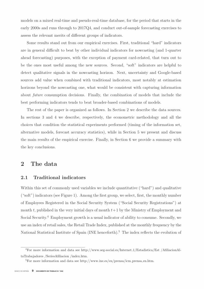
Resumen
Este documento se centra en la predicción a corto y medio plazo del consumo privado. La
selección de indicadores mensuales en tiempo real se realiza sobre la base de las variables
habituales (indicadores cualitativos versus cuantitativos) y de otras menos habituales.
Entre las variables de este último grupo se analizan las siguientes: i) variables proxy de la
incertidumbre económica y sobre las políticas económicas; ii) operaciones con tarjetas de
crédito, medidas tanto en TPV como en cajeros; iii) indicadores basados en búsquedas
de términos relacionados con el consumo obtenidas con la herramienta Google Trends. Se
estima un conjunto de modelos de frecuencias mixtas (mensual y trimestral) utilizando una
base de datos en tiempo real, y se realizan ejercicios empíricos para valorar la capacidad
predictiva de los diferentes grupos de indicadores. Los principales resultados son los
siguientes: i) los indicadores cuantitativos y los relativos al uso de tarjetas de crédito son
los que presentan mejor capacidad predictiva cuando se utilizan individualmente, y esta
mejora cuando se combinan; ii) a pesar de lo anterior, los indicadores de opinión son de
utilidad para captar señales cualitativas a muy corto plazo (en el horizonte del nowcast);
iii) los indicadores de Google y los de incertidumbre añaden información cuando se
combinan con los indicadores tradicionales, sobre todo en horizontes de proyección más
allá del nowcast, lo que sería consistente con el hecho de que estos indicadores pueden
contener información acerca de futuras decisiones de consumo; iv) la combinación de los
modelos que incluyen los indicadores que arrojan los mejores resultados tiende a mejorar
los resultados obtenidos con combinaciones más amplias de modelos.
Palabras clave: consumo privado, nowcasting, predicción macroeconómica, incertidumbre
económica, Google Trends.
Códigos JEL: E27, C32, C53.

BANCO DE ESPAÑA 7 DOCUMENTO DE TRABAJO N.º 1842
1 Introduction
Private consumption represents between 60% to 80% of an average OECD country gross
domestic product. Thus the importance for applied forecasters of having accurate estimates
of this GDP component in real-time. Benchmark data to approximate private households’
spending decisions are normally provided by the national accounts, and are available at the
quarterly frequency. Nevertheless, usually, there exists a significant publication lag, typi-
cally of 90 days after the quarter of reference ended. More timely data is usually published,
mostly, but not only, by National Statistical Institutes, in the form of economic indicators,
both covering quantitative information on observed spending decisions (so-called “hard”
indicators), and qualitative information provided by households’ surveys on consumer senti-
ment and consumption plans (so-called “soft” indicators). These standard leading indicators
of private consumption used by practitioners and academics alike, are typically available in
real-term with a 1 to 3 months delay, depending on the country, and are available at the
monthly frequency.
Nowdays, in addition, technological progress has enabled the development of other sources
of data usable for monitoring and forecasting real-time economic activity1 and, in particu-
lar, private consumption decisions, in many occasions from private sector sources, such as
Google Trends (see e.g. Choi and Varian, 2012), data on granular payment instruments,
like payment cards (see, e.g. Galbraith and Tkacz, 2018; Duarte et al., 2017), or indicators
based on textual analysis, including media news (see e.g. Backer et al., 2017). In our paper,
from a forecasting point of view, we analyze the information content of some of these new
source of information, but in a context in which we ascertain their value in conjunction with
traditional, more proven, sources of short-term information, such as the “hard” and “soft”
ones mentioned above.
In particular, among these new data sources we look, first, at data collected from
automated teller machines (ATMs), encompassing cash withdrawals at ATM terminals,
and points-of-sale (POS) payments with debit and credit cards, given the increasing and
widespread use of electronic payment systems by economic agents. Typically, electronically
1See Bok et al. (2017) or Baldacci et al. (2016).
recorded data are available in a quite timely fashion and are free of measurement errors (see
e.g. Galbraith and Tkacz, 2018, Duarte et al., 2017, Aprigliano et al., 217, Ardizzi et al.,

BANCO DE ESPAÑA 8 DOCUMENTO DE TRABAJO N.º 1842
2018, and the references quoted therein)2. Secondly, in line with a recent and very active
branch of the literature, we construct indicators of consumption behavior on the basis of
internet search patterns as provided by Google Trends. Over the past decade, the number
of Internet users has increased dramatically, and also their buying patterns. In this way
intentions to buy, as reflected in Internet searches of certain categories of goods and services,
might be useful to anticipate actual buying behavior. While indicators linked to income
reflect the ability to spend of consumers, and survey-based indicators capture the willingness
to spend, Google-searches-based variables based on consumption-related search queries may
provide a measure of consumers’ preparatory steps to spend (see Vosen and Schmidt, 2011,
2012; Choi and Varian, 2012). Finally, we use measures of economic and policy uncertainty,
in line with another recent strand of the literature that has highlighted the relevance of
the level of uncertainty prevailing in the economy for private agents’ decision-making (see,
among others, Backer et al., 2017). This is all the more relevant in the field of modeling
consumption decisions, as prescribed by the existing theoretical literature.
Building on these strands of the literature, in this paper we focus on nowcasting quar-
terly private consumption for the case of Spain, the fourth largest euro area economy. To
exploit the data in an efficient and effective manner, we build models that relate data at
the quarterly and monthly frequencies. We follow the modeling approach of Harvey and
Chung (2000).3 The mixture of frequencies, and the estimation of models at the monthly
frequency, implies combining variables that at the monthly frequency can be considered as
stocks with those being pure flows. The quarterly private consumption series cast into the
monthly frequency is a set of missing observations for the first months of the quarter (Jan-
2Other recent applications on the usefulness of credit card data are Bodas et al. (2018), that mimic
the standard retail sales index for Spain, or Dong et al. (2018), that use credit card transaction data for
measuring the economic effects of a series of protests on consumer actions and personal consumption.3Other approaches for modeling data at different sampling intervals are the methods based on regression
techniques (Chow and Lin, 1971, Guerrero, 2003), the MIDAS (MIxed DAta Sampling) approach (see Ghysels
et al., 2006, Clements and Galvao, 2008), the state space approaches of Liu and Hall (2001) and Mariano
and Murusawa (2003), or the ARMA model with missing observations of Hyung and Granger (2008).
uary and February, in the case of Q1) and the observed value assigned to the last month
of each quarter (say, March). Theoretically, the quarterly National Accounts series would
be obtained from monthly National Accounts series by aggregation of the three months of
a quarter (January to March) had them been available. We estimate such mixed-frequency
BANCO DE ESPAÑA 9 DOCUMENTO DE TRABAJO N.º 1842
models on a mixed real-time and pseudo-real-time database, for the period that starts in the
early 2000s and runs through to 2017Q4, and conduct out-of-sample forecasting exercises to
assess the relevant merits of different groups of indicators.
Some results stand out from our empirical exercises. First, traditional “hard” indicators
are in general difficult to beat by other individual indicators for nowcasting (and 1-quarter
ahead forecasting) purposes, with the exception of payment card-related, that turn out to
be the ones most useful among the new sources. Second, “soft” indicators are helpful to
detect qualitative signals in the nowcasting horizon. Next, uncertainty and Google-based
sources add value when combined with traditional indicators, most notably at estimation
horizons beyond the nowcasting one, what would be consistent with capturing information
about future consumption decisions. Finally, the combination of models that include the
best performing indicators tends to beat broader-based combinations of models.
The rest of the paper is organized as follows. In Section 2 we describe the data sources.
In sections 3 and 4 we describe, respectively, the econometric methodology and all the
choices that condition the statistical experiments performed (timing of the information set,
alternative models, forecast accuracy statistics), while in Section 5 we present and discuss
the main results of the empirical exercise. Finally, in Section 6 we provide a summary with
the key conclusions.
2 The data
2.1 Traditional indicators
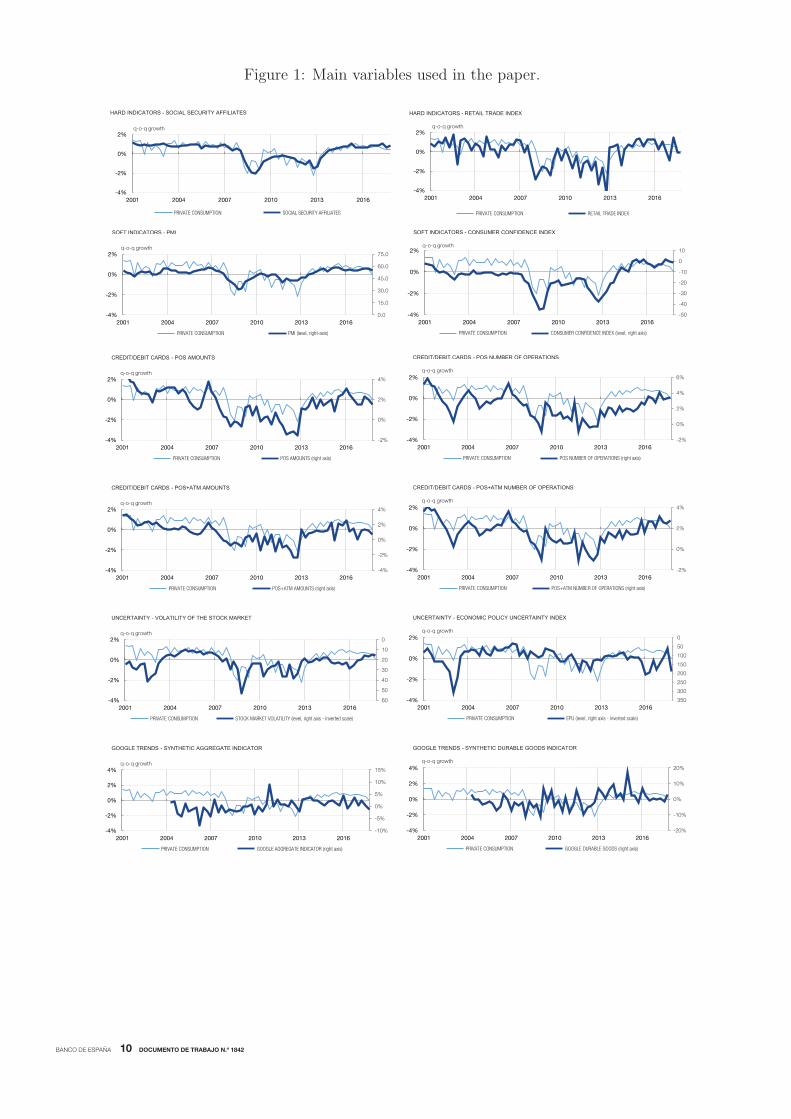
Within this set of commonly used variables we include quantitative (“hard”) and qualitative
(“soft”) indicators (see Figure 1). Among the first group, we select, first, the monthly number
of Employees Registered in the Social Security System (“Social Security Registrations”) at
month t, published in the very initial days of month t+1 by the Ministry of Employment and
Social Security.4 Employment growth is a usual indicator of ability to consume. Secondly, we
use an index of retail sales, the Retail Trade Index, published at the monthly frequency by the
National Statistical Institute of Spain (INE henceforth).5 The index reflects the evolution of
4For more information and data see http://www.seg-social.es/Internet 1/Estadistica/Est /AfiliacionAl-
taTrabajadores /SeriesAfiliacion /index.htm.5For more information and data see http://www.ine.es/en/prensa/icm prensa en.htm.
BANCO DE ESPAÑA 10 DOCUMENTO DE TRABAJO N.º 1842
Figure 1: Main variables used in the paper.
FUENTES: Bloomberg,
-2%
0%
2%
4%
6%
-4%
-2%
0%
2%
2001 2004 2007 2010 2013 2016
PRIVATE CONSUMPTION POS NUMBER OF OPERATIONS (right axis)
CREDIT/DEBIT CARDS - POS NUMBER OF OPERATIONS
q-o-q growth
-2%
0%
2%
4%
-4%
-2%
0%
2%
2001 2004 2007 2010 2013 2016
PRIVATE CONSUMPTION POS AMOUNTS (right axis)
q-o-q growth
CREDIT/DEBIT CARDS - POS AMOUNTS
-4%
-2%
0%
2%
2001 2004 2007 2010 2013 2016
PRIVATE CONSUMPTION SOCIAL SECURITY AFFILIATES
q-o-q growth
HARD INDICATORS - SOCIAL SECURITY AFFILIATES
-4%
-2%
0%
2%
2001 2004 2007 2010 2013 2016
PRIVATE CONSUMPTION RETAIL TRADE INDEX
HARD INDICATORS - RETAIL TRADE INDEX
q-o-q growth
-50
-40
-30
-20
-10
0
10
-4%
-2%
0%
2%
2001 2004 2007 2010 2013 2016
PRIVATE CONSUMPTION CONSUMER CONFIDENCE INDEX (level, right axis)
SOFT INDICATORS - CONSUMER CONFIDENCE INDEX
q-o-q growth
0.0
15.0
30.0
45.0
60.0
75.0
-4%
-2%
0%
2%
2001 2004 2007 2010 2013 2016
PRIVATE CONSUMPTION PMI (level, right-axis)
SOFT INDICATORS - PMI
q-o-q growth
-2%
0%
2%
4%
-4%
-2%
0%
2%
2001 2004 2007 2010 2013 2016
PRIVATE CONSUMPTION POS+ATM NUMBER OF OPERATIONS (right axis)
CREDIT/DEBIT CARDS - POS+ATM NUMBER OF OPERATIONS
q-o-q growth
-4%
-2%
0%
2%
4%
-4%
-2%
0%
2%
2001 2004 2007 2010 2013 2016
PRIVATE CONSUMPTION POS+ATM AMOUNTS (right axis)
q-o-q growth
CREDIT/DEBIT CARDS - POS+ATM AMOUNTS
0
50
100
150
200
250
300
350-4%
-2%
0%
2%
2001 2004 2007 2010 2013 2016
PRIVATE CONSUMPTION EPU (level, right axis - inverted scale)
UNCERTAINTY - ECONOMIC POLICY UNCERTAINTY INDEX
q-o-q growth
0
10
20
30
40
50
60-4%
-2%
0%
2%
2001 2004 2007 2010 2013 2016
PRIVATE CONSUMPTION STOCK MARKET VOLATILITY (level, right axis - inverted scale)
q-o-q growth
UNCERTAINTY - VOLATILITY OF THE STOCK MARKET
-20%
-10%
0%
10%
20%
-4%
-2%
0%
2%
4%
2001 2004 2007 2010 2013 2016
PRIVATE CONSUMPTION GOOGLE DURABLE GOODS (right axis)
GOOGLE TRENDS - SYNTHETIC DURABLE GOODS INDICATOR
q-o-q growth
-10%
-5%
0%
5%
10%
15%
-4%
-2%
0%
2%
4%
2001 2004 2007 2010 2013 2016
PRIVATE CONSUMPTION GOOGLE AGGREGATE INDICATOR (right axis)
q-o-q growth
GOOGLE TRENDS - SYNTHETIC AGGREGATE INDICATOR

BANCO DE ESPAÑA 11 DOCUMENTO DE TRABAJO N.º 1842
the sales and employment in the retail trade sector in Spain. Finally, we select the monthly
Services Sector Activity Indicator (published by INE6), given the significant weight of the
services sector in the Spanish economy (some 50% of GDP and 45% of employment). The
index measures the turnover and employment of services companies. The turnover captures
the amounts invoiced by each economic activity unit for the provision of services and sale of
goods.
As regards “soft” indicators, we focus on two. On the one hand, the Purchasing Manager’s
Index (PMI) of Services (elaborated by the private company Markit Economics), an index
based on monthly questionnaire responses from panels of senior purchasing executives (or
similar).7 On the other hand, we use the Consumer Confidence Indicator published each
month by the European Commission. This indicator is built on selected questions addressed
to consumers according to the Joint Harmonised EU Programme of Business and Consumer
Surveys.8
From a real-time perspective, Social Security Registrations, the PMI Services’ index, and
the Consumer Confidence Indicator are available with a one-month lag, while the Retail
Trade Index presents a lag of two months, and the Services Sector Activity Indicator is
published with a three months delay.9
2.2 Household’s payment cards data
Data on ATM withdrawals with payment cards — debit, delayed debit and credit cards
— (nominal amounts and number of operations), and payments made at POS (nominal
amounts spent and transactions) by residents, are made available by the main card service
providers (SERVIRED, Sistema 4B and Euro6000) to the Bank of Spain under strict confi-
dentiality conditions. They include both “card-not-present transactions” and “card-present”
transactions.10 Data can only be used for research purposes, and are received in aggregated
form (from anonymized original files). Card payments are a widespread means of payment
6See http://www.ine.es/en/prensa/iass prensa en.htm.7See https://ihsmarkit.com/products/pmi.html. The questions included in the PMI Services cover the
following economic variables: Business activity, new business, backlogs of work, prices charged, input prices,
employment, expectations for activity.8More details on the consumer confidence indicator as well as long time series can be found via the
following link: http://ec.europa.eu/economy finance/db indicators/surveys/index en.htm9All variables are available since, at least, the mid-1990s, with the exception of the Services Sector Activity
Indicator that starts in January 2002.10See Banco de Espana (2017).

BANCO DE ESPAÑA 12 DOCUMENTO DE TRABAJO N.º 1842
by Spanish consumers. In 2017, in Spain, these means of payments accounted for around
25% of private consumption. In addition, there are 51,000 ATMs and 1,800,000 POS, while
the number of payment cards is close to 80 million (for a population of 47 million inhab-
itants). Data in the Spanish case is available in yearly terms since 1996, on a quarterly
basis since 2006, and at the monthly frequency since 2009.11 As ATM/POS data are not
seasonally-adjusted, we use the TRAMO-SEATS software12 to remove the seasonal compo-
nent. In addition, nominal amounts are deflated by means of the headline Consumer Price
Index (CPI).
2.3 Uncertainty indicators
By now it is well established in the theoretical and empirical literature that heightened
economic uncertainty has the potential to harm economic activity, mainly through the effects
on households’ consumption, and firm’s investment, decisions (see, among others, Bloom,
2014). In the recent empirical literature, a number of works have dealt with the hurdle of
finding proxy measures of economic uncertainty, being the later a non-observable variable.
The extant studies tend to focus on one specific proxy or method, the most popular ones
being: (i) stock market volatility (see, e.g. Leahy and Whited, 1996; Bloom, 2009; Caggiano
et al, 2014); (ii) the variance of forecasters’ expectations, in many cases approximated by a
concept of disagreement (see, e.g., D’Amico and Orphanides, 2008; Bachmann et al., 2013;
Balta et al., 2013; Popescu and Smets, 2010) ; (iii) the frequency of news related to policy
uncertainty to form a proxy of policy uncertainty (Baker et al., 2016); (iv) the common
components of the volatility of the forecast errors from several macroeconomic time series (see
e.g. Jurado et al., 2013); on related grounds, some authors compute uncertainty measures
on the basis of real-time forecasting models (see, e.g. Scotti, 2016). In the current paper we
11Following the methodological approach described in section 3 of this paper, we use the data sampled
at the three different frequencies to generate an interpolated monthly time series for the time period of
reference for our study, using also as indicators the time series on “Cash and cash equivalents” (i.e. cash
and deposits: current accounts, savings accounts and deposits redeemable at up to 3 months’ notice), that
are available on a monthly basis for the whole period (see page 50 of Banco de Espana’s Statistical Bulletin
https://www.bde.es/f/ webbde/SES/Secciones/ Publicaciones/ InformesBoletinesRevistas/ BoletinEstadis-
tico/ 2018/Files/ie mayo2018 en.pdf).12See Gomez and Maravall (1996).

BANCO DE ESPAÑA 13 DOCUMENTO DE TRABAJO N.º 1842
focus on measures covering (i), (ii) and (iii). In particular, as regards (i) we use the volatility
of the Spanish Stock Market (IBEX-35)13, as regards (iii) we focus on the textual indicator
known as Economic Policy Uncertainty Index (EPU) for Spain elaborated by Baker, Bloom
and Davis (2015)14, and as to measures of disagreement, we construct several, standard
ones on the basis of: (a) private sector forecasts of private consumption and of consumption
prices; (b) European Commission’s consumer surveys, focusing on forward looking questions,
namely unemployment prospects.15
Specifically, regarding the forward-looking indicators on “Unemployment perspectives
over next 12 months”, we follow the approach of Bachmann et al. (2013) to construct
measures of uncertainty that exploit the information contained in the dispersion of responses.
Specifically, respondents to the above-mentioned questions can be grouped in three answers:
“decrease”, “unchanged” or “increase”. Let Frac+t denote the weighted fraction of consumers
in the cross section with “increase” responses at time t, and Frac−t the weighted fraction of
consumers with “decrease” responses. Then the “uncertainty indicator” is computed as
√Frac+t + Frac−t −
(Frac+t − Frac−t
)2
As to the measure of disagreement about private consumption among forecasters, we
take as starting point the month t cross section of current and one-year-ahead forecasts
about national accounts’ private consumption produced by analysts that do respond to the
“FUNCAS panel” of private sector analysts of the Spanish economy. FUNCAS is a private
sector institute that has been compiling forecasters’ views since 1999.16 At each point in time,
the measure of “disagreement” is computed as the standard deviation of such cross-section
of n forecasters from the mean (“consensus”) forecast CA,1n
∑i=1 n
(Ci − CA
)2
. Given that
each analyst i provides growth rates of two fixed-event forecasts (current and year-ahead) m
months ahead, it is necessary to correct each time-t value by the fact that it is computed on
an evolving information set. For that, we follow the methodology of Dovern et al. (2012).
13As computed every month by the International Center for Decision Making (ICDM) and IESE Business
School: see https://blog.iese.edu/icdm/que-es-el-i3e/.14Available for the period that starts in January 2001.15See Gil et al. (2017) and Ghirelli et al. (2018).16For more information on the panel see https://www.funcas.es/Indicadores/Index.aspx.
BANCO DE ESPAÑA 14 DOCUMENTO DE TRABAJO N.º 1842
2.4 Internet search query data (Google Trends)
We construct indicators of private consumption based on internet search data queries through
Google Trends. Google Trends provides an index of the relative volume of search queries
conducted through Google. The application provides aggregated indexes of search queries
which are classified into categories and sub-categories using an automated classification en-
gine. Google Trends provides a time series index of the volume of queries users enter into
Google in a given geographic area. The query index is based on query share: the total
query volume for the search term in question within a particular geographic region divided
by the total number of queries in that region during the time period being examined. The
maximum query share in the time period specified is normalized to be 100, and the query
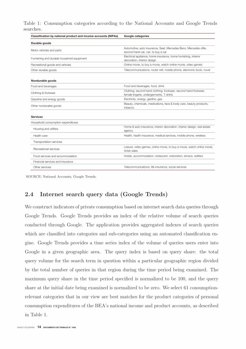
share at the initial date being examined is normalized to be zero. We select 61 consumption-
relevant categories that in our view are best matches for the product categories of personal
consumption expenditures of the BEA’s national income and product accounts, as described
in Table 1.
Table 1: Consumption categories according to the National Accounts and Google Trendssearches.
Classification by national product and income accounts (NIPAs) Google categories
Durable goods
Motor vehicles and parts
Furnishing and durable household equipment
Recreational goods and vehicles
Other durable goods
Nondurable goods
Food and beverages
Clothing & footwear
Gasoline and energy goods
Other nondurable goods
Services
Household consumption expenditures
Housing and utilities
Health care
Transportation services
Recreational services
Food services and accommodation
Financial services and insurance
Other services
Hotels, accommodation, restaurant, restoration, terrace, welfare
Telecommunications, life insurance, social services
Home & auto insurance, interior decoration, interior design, real estate
agency
Health, health insurance, medical services, mobile phone, wireless
Leisure, video games, online movie, to buy a movie, watch online movie,
ticket sales
Food and beverages, food, drink
Clothing, second hand clothing, footwear, second hand footwear,
female lingerie, undergarments, T-shirts
Electricity, energy, gaoline, gas
Beauty, chemicals, medications, face & body care, beauty products,
tobacco
Automotive, auto insurance, Seat, Mercedes Benz, Mercedes offer,
second hand car, car, to buy a car
Electrical appliance, home insurance, home furnishing, interior
decoration, interior design
Online movie, to buy a movie, watch online movie, video games
Telecommunications, router wifi, mobile phone, electronic book, novel
SOURCE: National Accounts, Google Trends.

BANCO DE ESPAÑA 15 DOCUMENTO DE TRABAJO N.º 1842
It is possible to obtain raw data from Google Trends for the period starting in 2004,
on a monthly basis. Data are non-seasonally adjusted, and thus seasonality is removed by
using the TRAMO-SEATS software.17 The so corrected series are summarized in groups,
following a conceptual approach, as in Table 1, in order to calculate synthetic indicators of (i)
durable goods’ consumption, (ii) non-durable goods’ consumption, and (iii) services goods’
consumption; (iv) an aggregate of all consumption categories. The weights used to combine
the Google indicators are calculated on the basis of the classification tables of consumption
expenditure by purpose of the National Accounts (COICOP tables). In addition, we also
aggregate the 61 Google Trends indicators using principal components analysis, as it is
standard in the literature (see, e.g., Vosen and Schmidt, 2011, 2012).18
2.5 A first, standard look at the explanatory power of the data
In this section we present an exploratory analysis of the contribution of non-traditional
indicators by means of standard bridge equations.19 First, we estimate an equation for real
private consumption Ct, in which households’ disposable income, the interest rate and lagged
consumption are included as explanatory variables, to provide a simple baseline. Then, we
augment the latter with short-term indicators. Let Xit denote the corresponding stationary
short-term monthly indicator i, time-averaged to the quarterly frequency. Then, we estimate
the following model (by ordinary least squares)
Δ log(Ct) = α1 + α2Δ log(Ct−1) + α3Δ log(INCt−1) + α4rt + β1X1t + β2X2t + . . .+ εt
where INC denotes disposable income and rt the short-term interest rate. In columns [1]
to [5] of Table 2 we first show the results of including in the bridge equation two indicators
from each block at a time, namely quantitative, qualitative, credit cards, uncertainty, and
Google Trends. In all cases, both or at least one of the indicators of each block turns out
17The data is downloaded and seasonally-adjusted following a pseudo-real-time scheme, as follows. First,
time series are downloaded by sub-samples using Google Trends, so that they can be accommodated to
the timing convention and structure of the forecasting exercise described in Section 4. This amounts to
downloading sequentially the data for the time period January 2004 to January 2008, January 2004 to
February 2008, ..., January 2004 to December 2017. In a second step, each data series for each sub-sample
is seasonally-adjusted.18See also Gotz and Knetsch (2017). For a critical view, see, among others, Liu (2016).
19For comparability, we follow closely the approach by Vosen and Schmidt (2011, 2012).

BANCO DE ESPAÑA 16 DOCUMENTO DE TRABAJO N.º 1842
to be relevant to explain changes in consumption in a given quarter. Nevertheless, when we
include in the regression one indicator of each block (column [6]), the “Hard” and the POS
ones are the only ones that turn out to be significant from a statistical point of view. When
the “Hard” indicator is excluded (column [7]), the “Soft” and the Google-Trends indicators
capture part of the variance of consumption that the former indicator was able to explain.
Thus, in this modeling framework, at the quarterly frequency, and not giving any publi-
cation advantage to any data source, “hard” and payment cards’ indicators seem to dominate
the rest. In what follows, we further explore the information content of the different sources
of information, but in a more comprehensive set-up in which the advanced information with
which these variables are available may play a role in its potential usefulness for the ap-
plied, real-time forecaster. Beyond timeliness, some indicators may have anticipatory power,
insofar as they capture information on agents’ expectations (like the uncertainty and Google-
Trend-based ones).
Table 2: Preliminary exploration: regressions of Δ log(Ct) on its own lag and differentindicators. P-Values.
p-values [1] [2] [3] [4] [5] [6] [7]Sample: 2001Q1-2016Q4
Constant 0.060 ∗ 0.052 ∗∗ 0.000 ∗∗∗ 0.047 ∗∗ 0.288 0.280 0.001 ∗∗∗Interest rate: Euribor 3-monthsa 0.635 0.674 0.829 0.513 0.370 0.523 0.782Households’ disposable incomeb 0.952 0.564 0.267 0.338 0.265 0.761 0.487Lagged Δ log(Ct) 0.772 0.100 ∗ 0.002 ∗∗∗ 0.000 ∗∗∗ 0.000 ∗∗∗ 0.660 0.2969Short-term Indicators:“Hard”: Social Security Registrationsb 0.000 ∗∗∗ 0.010 ∗∗“Hard”: Retail Trade Indexb 0.020 ∗∗“Soft”: PMI-Servicesc 0.007 ∗∗∗ 0.258 0.000 ∗∗∗“Soft”: Consumers’ Confidence Indexc 0.162Credit cards: POS amounts (real)b 0.003 ∗∗∗ 0.007 ∗∗∗ 0.000 ∗∗∗Credit cards: POS number of transactionsb 0.252Uncertainty: Stock market volatilityc 0.0951 ∗ 0.872 0.970Uncertainty: Economic Policyd 0.0000 ∗∗∗Google Trends: Durable Goodsb 0.037 ∗∗ 0.192 0.086 ∗Google Trends: Non-durable Goodsb 0.207R-squared statistic 0.72 0.62 0.60 0.51 0.49 0.74 0.71
Notes:a. Deviation from trend (HP-filter).b. Δ log(•).c. Variable in levels.d. Δ(•).

BANCO DE ESPAÑA 17 DOCUMENTO DE TRABAJO N.º 1842
3 The mixed-frequencies, times series models
The starting point of the modeling approach is to consider a multivariate Unobserved Com-
ponents Model known as the Basic Structural Model (BSM, Harvey, 1989)20. A given
(seasonally-adjusted) time series is decomposed into unobserved components which are mean-
ingful from an economic point of view (trend, Tt, and irregular, et). Equation (1) displays
a general form, where t is a time sub-index measured in months, zt denotes the variable in
National Accounts terms expressed at a quarterly sampling interval for our objective time
series (private consumption), and ut represents the vector of monthly indicators.
⎡⎣ zt
ut
⎤⎦ = Tt + et (1)
The general consensus in this type of multivariate models in order to enable identifiabil-
20The exposition in this section follows closely Pedregal and Perez (2010) and Harvey and Chun (2000).
For some examples of applications of this approach to the field of forecasting see, among many others, Grassi
et al. (2015), Moauro (2014), or Durbin and Koopman (2012), and the references quoted therein.
ity is to build SUTSE models (Seemingly Unrelated Structural Time Series). This means
that components of the same type interact among them for different time series, but are
independent of any of the components of different types. In addition, statistical relations
are only allowed through the covariance structure of the vector noises, but never through
the system matrices directly. This allows that trends of different time series may relate to
each other, but all of them are independent of the irregular components. The full model is
a standard BSM that may be written in State-Space form as
xt = Φxt−1 + Ewt (2)⎡⎣ zt
ut
⎤⎦ =
⎡⎣ H
Hu
⎤⎦xt +
⎡⎣ εt
vt
⎤⎦ (3)
where εt ∼ N(0,Σε) and vt ∼ N(0,Σvt). The system matrices Φ, E, H and Hu in
equations (2)-(3) include the particular definitions of the components and all the vector noises
have the usual Gaussian properties with zero mean and constant covariance matrices (εt and
vt are correlated among them, but both are independent of wt). The particular structure
of the covariance matrices of the observed and transition noises defines the structures of
correlations among the components across output variables. The mixture of frequencies,
and the estimation of models at the monthly frequency, implies combining variables that at

BANCO DE ESPAÑA 18 DOCUMENTO DE TRABAJO N.º 1842
the monthly frequency can be considered as stocks with those being pure flows. Thus, given
the fact that our objective variables are observed at different frequencies, an accumulator
variable has to be included
Ct =
⎧⎨⎩
0, t = first month of the quarter
1, otherwise(4)
so that the previous model turns out to be⎡⎣ zt
xt
⎤⎦ =
⎡⎣ Ct ⊗ I HΦ
0 Φ
⎤⎦⎡⎣ zt−1
xt−1
⎤⎦+
⎡⎣ 1 HE
0 E
⎤⎦⎡⎣ εt
wt
⎤⎦ (5)
⎡⎣ zt
ut
⎤⎦ =
⎡⎣ I 0
0 Hu
⎤⎦⎡⎣ zt
xt
⎤⎦+
⎡⎣ 0
I
⎤⎦ vt (6)
Given the structure of the system and the information available, the Kalman Filter and
Fixed Interval Smoother algorithms provide an optimal estimation of states. Maximum
Table 3: High frequency variables used in the study and information flow: information
available at each nowcasting origin.
1st month
2nd month
3rd month
1st month
2nd month
3rd month
1st month
2nd month
3rd month
1st month
2nd month
3rd month
1st month
2nd month
3rd month
1st month
2nd month
3rd month
Private consumption (QNA)
Social security registrations
Retail trade index
Services activity index
PMI. Services
Consumers confidence index
Credit cards - ATMs
Credit cards - POSs
Disagreement - consumption
Disagreement - inflation
Unemploymeny expectations
Economic policy uncertainty
Stock market volatility
Google Trends
… m3 (3rd month of the quarter)
Previous quarter Current quarter
… m1 (1st month of the quarter)
Previous quarter Current quarter
Information available at nowcasting time…
… m2 (2nd month of the quarter)
Previous quarter Current quarter
a. Dark colour in a horizontal line denotes lack of availability of the indicator in a particular point in time within the quarter.
likelihood in the time domain provides optimal estimates of the unknown system matrices,
which in the present context are just covariance matrices of all the vector noises involved in
the model. The use of the selected modeling approach, allows the estimation of models with
unbalanced data sets, i.e. input variables with different sample lengths, an issue relevant
for the application at hand given the different timing of publication of incoming monthly
indicators.

BANCO DE ESPAÑA 19 DOCUMENTO DE TRABAJO N.º 1842
4 The empirical exercise
4.1 Timing of the (pseudo) real-time exercise
We build up a real-time database for the target variable, quarterly private consumption
as measured by the National Accounts, for the period 1995Q1-2017Q4. The size of the
sample for our empirical exercises, though, is restricted by the availability of some of the
monthly indicators, in particular as regards Google Trends, the EPU index, and the Services
Sector Activity Indicator, available for the sample starting in January 2004, January 2001,
and January 2002, respectively. As regards the indicator variables we could not replicate
a truly real-time dataset, so we proceeded to built up a pseudo real-time one, namely we
adjusted for each point in time (month) the information set that had been available given
the timing rules that we describe in the next paragraph. It is worth mentioning that the
indicators that we use are not revised, which means that the pseudo-real-time approximation
should be a fair representation of data available in real-time. The only discrepancy may arise
from seasonal-adjustment. While we seasonally-adjust the series that are published on non-
seasonally-adjusted terms following our pseudo-real-time approach, we take official series
that are published in a seasonally-adjusted form as the latest available vintage of official
data.
As regards the rules governing the timing of availability of the data, this is illustrated in
Table 3. At the time the first month of each quarter (denoted by m1 in the table) is over (i.e.
at the very beginning of the subsequent month) the official quarterly national accounts has
not yet been released by the statistical agency. Within the group of quantitative indicators,
only employment (Social Security Registrations) is available at that moment of time, while
the most recent figure for the Retail Trade Index does correspond to the second month of the
previous quarter, and the Services Activity Indicator presents a lag of two months. In turn,
“soft” indicators are published more timely, and at m1 they both already cover the whole
t − 1 quarter. The same happens with the uncertainty indicators computed from surveys,
while the EPU index presents a delay of two months. The more timely indicators are the
payment cards ones, the volatility of the stock market, and the internet-based variables.
Given their daily production process, they would be available to the real-time forecasters at
the very beginning of the next month (what we denote by m1).

BANCO DE ESPAÑA 20 DOCUMENTO DE TRABAJO N.º 1842
of all possible combinations, that were chosen for its better forecasting performance.21 In
particular, we focus on the following models for quarterly private consumption:
• Models including indicators of only one group: (i) Quantitative (“hard”) indicators;
(ii) Qualitative (“soft”) indicators; (iii) Payment cards: aggregate of POS and ATM
- amounts; (iv) Payment cards: aggregate of POS and ATM - number of operations;
(v) Uncertainty indicators: Stock Market Volatility and EPU; (vi) Google Trends:
aggregate of all indicators; (vii) Google Trends: durable goods aggregate (with one
lag).
• Models including indicators of different groups: (i) Quantitative and qualitative; (ii)
Quantitative and POS-ATM amounts; (iii) Quantitative and Uncertainty; (iv) Quanti-
tative and Google Trends (aggregate); (v) Quantitative and Google Trends (durables,
with one lag).
• Combination of models that do include indicators of only one group: (i) Suite of 30
models22; (ii) “Hard” and aggregate of POS and ATM amounts; (iii) “Hard”, aggregate
of POS and ATM amounts, and “Soft”; (iv) “Hard” and “Soft”; (v) “Hard” and Google.
We perform a rolling forecasting exercise in which the selection of the forecast origin
and the information set available at each date are carefully controlled for. In particular we
evaluate the forecasts generated from three forecast origins per quarter (m1, m2, m3) for
the time window 2008Q1 to 2017Q4. This makes up to 40 projections from each forecast
origin, and a total of 120 projections at each forecast horizon. In addition, we break down
the sample in two sub-samples, to broadly capture the most recent economic crisis period
(2008-2012), and the subsequent economic recovery (2013-2017).
21All the results are available upon request.22These models include those described in the two groups before (plus a version of each one in which the
variables are included with 1 lag), and the additional bilateral combinations of “Hard” and other indicators
not covered above (plus a version of each one in which the variables are included with 1 lag).
4.2 Alternative models and comparison criteria
In order to test the relevant merits of each group of indicators, as mentioned above, we
consider several models, that differ in the set of indicators included in each one. We esti-
mate models that include indicators from each group at a time, several groups at a time,
and different combinations of individual models. We only provide results for a selection

BANCO DE ESPAÑA 21 DOCUMENTO DE TRABAJO N.º 1842
As a mechanical benchmark we use a random walk model, whereby we repeat in future
quarters the latest quarterly growth rate observed for private consumption. Beyond being
a usual benchmark in statistical works, the random walk model of consumption is a clas-
sical one from a theoretical point of view (see the seminal paper of Hall, 1978). Rational
expectations together with the hypothesis of constant expected real interest rates implies
that any changes in consumption should be unpredictable, i.e. evolve as a random walk,
which is consistent with the permanent income hypothesis of consumption. According to
the random walk model for consumption, no information known to the consumer when the
consumption choice at t was made can have any predictive power for how consumption will
change between period t and t+ 1 (or for any date beyond t+ 1).23
We focus on the forecast performance at the nowcasting horizon (current quarter), but
also explore forecasts at 1 to 4 quarters-ahead from each one of the current quarter forecast
origins (m1, m2 and m3).
As regards forecasting performance statistics, we present three standard quantitative
measures. First, the ratio of the Root Mean Squared Errors (RMSE) of the different alter-
native models with respect to the quarterly random walk alternative. Second, we also look
at the Diebold and Mariano test (using the finite sample modification of Harvey et al., 1997),
and test for the null hypothesis of no difference in the accuracy of two competing forecasts.
The Diebold-Mariano test could be biased when parameter uncertainty is taken into account
(see for example Clark and McCraken, 2001). We make sure that a reasonable proportion
of the sample is employed when the first out-of-sample forecast is computed to reduce the
bias generated by ignoring parameter uncertainty (the forecasting exercise is performed on
the moving window 2008-2017, while the full sample covers 2001-2017). Finally, we compare
model/indicator performance by means of the Pesaran-Timmermann test (see Pesaran and
Timmermann, 1992), that determines the accuracy in predicting the change in direction of
a time series, i.e. its directional accuracy.
In all cases, errors are computed as the difference of the nowcast/forecast value from two
vintages of data: the first release of each quarterly figure, and the 2018Q1 vintage of data.
As illustrated by Figure 2, differences can be quite significant depending on the reference
23As regards the link with the empirical specification chosen, please notice that the prescriptions of the
usual theoretical sugmodels are derived for variables that fluctuate in a stationary fashion around a deter-
ministic steady-state.

BANCO DE ESPAÑA 22 DOCUMENTO DE TRABAJO N.º 1842
Figure 2: Quarterly private consumption: first release of each quarterly figure versus the2018Q1 data vintage (quarter-on-quarter growth rates). 2008Q1-2017Q4 sample.
2.5
2.0
1.5
1.0
0.5
0.0
0.5
1.0
1.5
2008q1 2009q1 2010q1 2011q1 2012q1 2013q1 2014q1 2015q1 2016q1 2017q1
First release 2018Q1 vintage of data
point taken to compute the forecast error. While first released figures are the ones of concern
from the perspective of a real-time forecaster, they tend to be produced with a more limited
informational base than subsequent data publications. From this perspective subsequent
revisions of initially published figures can be sizeable, beyond changes due to methodological
improvements of statistical sources.24
5 Results
The main results of the empirical exercises are shown in Table 4, that display RMSE statistics
of each model with respect to the quarterly random walk alternative, figures 3 and 4, that
provide an illustration of the behavior of model nowcasts/forecasts around turning points,
figures 5 and 6, presenting RMSEs for selected models, and in “good” vesus “bad” times,
tables 5, 6, 7, that show pairwise RMSEs and Diebold-Mariano statistics, and tables 8 and
24For a cross-country overview of revisions to quarterly national accounts data see, for example,
http://www.oecd.org/sdd/na/revisions-of-quarterly-gdp-in-selected-oecd-countries.htm
9, that present Pesaran-Timmermann tests. Forecast errors in all cases are computed using
the first released figure. Additional tables based on the 2018Q1 vintage are presented in
Appendix A (tables A.1, A.2, A.3, A.4, A.5, and A.6).

BANCO DE ESPAÑA 23 DOCUMENTO DE TRABAJO N.º 1842
First, from tables 4 (relative RMSEs) and 5 to 7 (Dieblod-Mariano tests), the following
results can be highlighted. As regards models that use only indicators from each group (first
panel of the table), the ones that use quantitative indicators and payment cards (amounts)
tend to perform best than the others at the nowcasting and, somewhat less so, forecasting
(1-quarter- and 4-quarters-ahead) horizons. Relative RMSE are in almost all cases below
one, even though from a statistical point of view they are only different from quarterly
random walk nowcasts and forecasts in a few instances. In general, the other models do not
beat systematically the quarterly random walk alternative. The two main exceptions are
the model with qualitative indicators for the nowcasting horizons, and the Google-Trends-
based ones for the longer-horizon forecasts. The latter results might be consistent with the
prior that Google-based indicators deliver today information on steps to prepare purchases
in the future. Lastly, it is worth mentioning that nowcast/forecast accuracy does not always
improve monotonically as the information set expands, i.e. as we move from nowcast/forecast
origins m1 to m3. This is explained by the real-time nature of the information set used in
each case. Following the standard publication calendar, at m2-time the quarterly figure
of private consumption corresponding to the previous quarter is published. This has two
implications. On the one hand, the quarterly random walk alternative moves from a situation
in which the reference was the t − 2 figure to one in which the t − 1 quarter is used. On
the other hand, quarterly data corresponding to previous quarters tend to be revised at m2,
which may affect the estimation of models in real-time, and eventually the accuracy of the
generated nowcasts/forecasts, or at least the comparability of estimations based on different
information sets. The revision of past, quarterly national accounts figures is quite apparent
when going through the different pannels of figures 3 and 4 in a chronological order.
Second, in the middle panel of Table 4 we show the results of the estimation of models that
include quantitative indicators while adding, in turn, variables from the other groups (qual-
itative, payment cards - amounts, uncertainty, Google-Trends-based). The improvement in
nowcast accuracy is not generalized when adding more indicators, with the exception of the
“soft” ones (m1 and m3 origins). Nonetheless, there is a significant improvement for longer
forecast horizons of expanding the baseline model. In particular, for the 4-quarters-ahead
one, uncertainty and Google-based indicators add significant value to the core “hard”-only-
based model.
Finally, as regards the third panel of results of Table 4, and the corresponding Diebold-
Mariano test results in tables 5 to 7, it seems clear that the combination (average) of models

BANCO DE ESPAÑA 24 DOCUMENTO DE TRABAJO N.º 1842
with individual groups of indicators improves the forecasting performance in all cases and
at all horizons. Most notably, the combination of the forecasts of models including quan-
titative indicators with those with payment cards (amounts), delivers, in general, the best
nowcasting/forecasting performance at all horizons. At the same time, adding the “soft”
forecasts seems to add value in the nowcasting phase, when more information for the current
quarter is available (m2 and m3 origins). In turn, the combination of a broad set of models
(first line of the panel) produces the lowest RMSE relative to the quarterly random walk at
the four quarters ahead forecast horizon. Nevertheless, the bilateral DM-test results with
respect to combinations of simpler models do not tend to be, in general, significantly differ-
ent from zero from a statistical point of view. In addition, according to this metric, also the
models with only quantitative, qualitative and payment cards indicators individually, beat
the combination of the broad set of models at the nowcasting horizons.
Regarding the ability of models to correctly anticipate the sign of changes in private
consumption (Pesaran-Timmerman test) we present two exercise. In the first one (shown
in Table 8), the aim is to capture the sign of the growth rate of private consumption (i.e.
whether it is positive or negative). In the second one (shown in Table 9), in turn, we provide
results for the percentage of correctly anticipated accelerations or decelerations in private
consumption, i.e. the second derivative, that tends to be of more interest to the applied fore-
caster. As regards the first exercise, the results shown in Table 8 indicate that: (i) the model
that only includes “soft” indicators dominates the other at the nowcasting horizons, with
gains of some 5% of correctly predicted signs; (ii) for longer forecast horizons, models based
on quantitative and payment cards indicators tend to present a better record, also when
combined with qualitative indicators. As to the second exercise (Table 9), the following re-
sults are worth highlighting: (i) At the nowcasting horizons, models using quantitative and,
to a lesser extent, payment cards indicators (amounts) are the best at anticipating acceler-
ations/decelerations in private consumption growth; (ii) payment card indicators (amounts
and numbers) present a good behaviour for foreasting horizons; (iii) Google-Trends based in-
dicators (durable goods) are the best performers at long forecast horizons (4-quarters-ahead)
within the group of single-indicator models.
Turning again to figures 3 and 4, some additional facts can be highlighted. First, as
regards figure 3, that shows the results for the double-dip of private consumption (and
economic activity, more generally), the model selected for the illustration (with quantitative
indicators) adequately capture, and subsequently adapt to, the downturn in consumption
BANCO DE ESPAÑA 25 DOCUMENTO DE TRABAJO N.º 1842
that burst in the first quarter of 2008. Second, as of the second quarter of 2009 the recovery
starts to be signalled for the subsequent quarters, but forecasts for more distant horizons tend
to be flat, which ex post was consistent with the observed double-dip of economic activity
that occurred as of 2011. All this said, forecasts for longer horizons during the 2008Q1 to
2009Q4 period perform relatively poorly. Thus, in figure 4, we show the behaviour of the
selected model for the period that encompasses the end of the second recession (2011) and
the start of the economic recovery phase (end of 2013). It is clear from the figure that the
model starts signalling the turn (recovery phase) as of 2011Q4, despite the observed negative
growth rates of private consumption on which the information set conditions at that moment.
Discrepancies with first-released outcomes, particularly at forecasting horizons, tend to be
smaller in the 2013 recovery phase than in the crisis period. This is also the case for the
subsequent years, not shown in the figure for the sake of brevity. The worst nowcast/forecast
performance in crisis times is illustrated by figure 6, in which we show relative RMSEs of
different models in the crisis (2008-2012) and recovery (2013-2017) phases of the cycle, with
respect to the whole sample.
Past data revisions do not appreciably affect the main results described above. This is
clear from the tables in Appendix A that present all the results for nowcast and forecast
errors computed on the basis of the 2018Q1 vintage of data, instead of the first released
figure. Interestingly, though, past data revisions in our real-time setting somehow affect
the interpretation of some of the results, in particular as regards the expected increase in
accuracy when the information set expands and, less so, the expected reduction in forecast
accuracy for longer-horizons. This is illustrated in Figure 5, where we present the RMSEs of
some selected models: the quarterly random walk, the model with only “hard” indicators,
the combination of “hard” and payment cards (amounts)-based models, and the broader
combination with a set of 30 models. The RMSE of each model does not get monotonically
reduced as we move from the nowcast/forecast originm1 tom2 and then tom3. As mentioned
above, this might be partly related to the change on the past private consumption data that
enters the information set at each point in time, including in some cases significant past data
revisions.

BANCO DE ESPAÑA 26 DOCUMENTO DE TRABAJO N.º 1842
6 Conclusions
We estimate a suite of mixed-frequency models on an (almost) real-time database for the
period January 2001 - December 2017, and conduct out-of-sample forecasting exercises to
assess the relevant merits of different groups of indicators. The selection of indicators is
guided by the standard practice (“hard” and “soft” indicators), but also expand this practice
by looking at non-standard variables, namely: (i) a suite of proxy indicators of uncertainty,
calculated at the monthly frequency; (ii) two additional sets of variables that are sampled at a
much lower frequency: payment card transactions and indicators based on search query time
series provided by Google Trends. The latter set of indicators is based on factors extracted
from consumption-related search categories of the Google Trends application. Our study
shows that, even though traditional indicators make a good job at nowcasting and forecasting
private consumption in real-time, novel data sources add value, most notably those based on
payment cards-related, but also, to a lesser extent, Google-based and uncertainty indicators
when combined with other sources.

BANCO DE ESPAÑA 27 DOCUMENTO DE TRABAJO N.º 1842
References
Aprigliano, V., G. Ardizzi, and L. Monteforte (2017), “Using the payment system data to
forecast the Italian GDP”, Bank of Italy, Working Paper 1098.
Ardizzi, G., S. Emiliozzi, J. Marcucci, and L. Monteforte (2018), “News and consumer card
payments”, Bank of Italy, mimeo.
Bachmann, R., S. Elstener and E. Sims (2013), “Uncertainty and Economic Activity: Evi-
dence from Business Survey Data”, American Economic Journal: Macroeconomics, 5,
pp. 217-249.
Baker, S., N. Bloom and S. Davis (2016), “Measuring Economic Policy Uncertainty”, The
Quarterly Journal of Economics, 131, pp. 1593–1636.
Baldacci, E., D. Buono, G. Kapetanios, S. Krische, M. Marcellino, G. L. Mazzi, and F.
Papailias (2016), “Big Data and Macroeconomic Nowcasting: from data access to
modelling”, Eurostat Statistical Book.
Balta, N., E. Ruscher and I. Valdes Fernandez (2013), “Assessing the impact of uncertainty
on consumption and investment”, European Commission, Quarterly Report on the
Euro Area, 12, pp. 7-16.
Banco de Espana (2018), “Memoria anual sobre la vigilancia de las infraestructuras de
los mercados financieros 2017”. Available at: https://www.bde.es/f/webbde /Sec-
ciones/Publicaciones/PublicacionesAnuales/ MemoriaAnualSistemasPago/17/MAV2017.pdf
Bloom, N. (2014). “Fluctuations in Uncertainty”, Journal of Economic Perspectives, 28,
pp. 153 176.
Bloom, N. (2009). “The impact of uncertainty shocks”, Econometrica, 77, pp. 623 685.
Bodas, D., J. R. Garcıa, J. Murillo, M.Pacce, T. Rodrigo, P. Ruiz, C. Ulloa, J. Romero,
and H. Valero (2018), “Measuring retail trade using card transactional data”, BBVA
Research Working Paper 18/03, Madrid, Spain.
Bok, B., D. Caratelli, D. Giannone, A. M. Sbordone, and A. Tambalotti (2017), “Macroe-
conomic Nowcasting and Forecasting with Big Data”, Federal Reserve Bank of New
York, Staff Report 890.

BANCO DE ESPAÑA 28 DOCUMENTO DE TRABAJO N.º 1842
Bontempi, M. E., R. Golinelli, and M. Squadrani (2016), “A new index of uncertainty based
on Internet searches: a friend or foe of other indicators?”, Quaderni Working Paper
DSE No 1062, Department of Economics, Universita di Bologna.
Caggiano, G., E. Castelnuovo, and N. Groshenny (2014), “Uncertainty Shocks and Un-
employment Dynamics in U.S. Recessions”, Journal of Monetary Economics, 67, pp
78-92.
Carriere-Swallow, Y. and F. Labbe (2013), “Nowcasting with Google trends in an emerging
market”, Journal of Forecasting, 32, pp. 289-298.
Choi, H. and H. Varian (2012), “Predicting the present with Google Trends”, Economic
Record, 88, pp. 2-9.
Chow, G. and A. Lin (1971), “Best Linear Unbiased Interpolation, Distribution, and Ex-
trapolation of Time Series by Related Series”, The Review of Economics and Statistics,
53, pp. 372-75.
Clark, T.E. and M.W. McCracken (2001), “Tests of equal forecast accuracy and encom-
passing for nested models”, Journal of Econometrics, 105, pp 85–110.
Clements, M. and A. Galvao (2008), “Macroeconomic Forecasting With Mixed-Frequency
Data”, Journal of Business and Economic Statistics, 26, pp 546-554.
D’Amico, S. and A. Orphanides (2008), “Uncertainty and disagreement in economic fore-
casting”, Finance and Economics Discussion Series 2008-56, Board of Governors of the
Federal Reserve System.
Degrer, Ch. and K. A. Kholodilin (2013), “Forecasting private consumption by consumer
surveys”, Journal of Forecasting, 32, pp. 10-18.
Dong, X., J. Meyer, E. Shmueli, B. Bozkaya, and A. Pentland (2018), “Methods for quan-
tifying effects of social unrest using credit card transaction data”, EPJ Data Science,
7:8. https://doi.org/10.1140/epjds/s13688-018-0136-x.
Dovern, J., U. Fritsche and J. Slacalek (2012), “Disagreement among forecasters in G7
countries”, The Review of Economics and Statistics, 94, pp. 1081-1096.

BANCO DE ESPAÑA 29 DOCUMENTO DE TRABAJO N.º 1842
Duarte, C., P. M. M. Rodrigues, and A. Rua (2017), “A mixed frequency approach to the
forecasting of private consumption with ATM/POS data”, International Journal of
Forecasting, 33, pp. 61-75.
Durbin, J., and S. J. Koopman (2012), “Time Series Analysis by State Space Methods”,
Oxford University Press, Oxford, Second Edition.
Edelman, B. (2012), “Using Internet data for economic research”, Journal of Economic
Perspectives, 26, pp. 189-206.
Einav, L. and J. D. Levin (2013), “The data revolution and economic analysis”, Working
Paper 19035, NBER Working Paper Series, National Bureau of Economic Research.
Faberman, J. and M. Kudlyak (2016), “What does online job search tell us about the labor
market?”, Economic Perspectives, Federal Reserve Bank of Chicago, 1.
Fondeur, Y. and F. Karame (2013), “Can Google data help predict French youth unem-
ployment?”, Economic Modelling, 30, pp. 117-125.
Galbraith, J.W. and G. Tkacz (2018), “Nowcasting with payments system data”. Interna-
tional Journal of Forecasting, 34, pp. 366-376.
Gil, M., J. J. Perez and A. Urtasun (2017), “Macroeconomic Uncertainty: Measurement and
Impact on the Spanish Economy”, Bank of Spain Economic Bulletin 1/2017, Analytical
Articles (2 February 2017).
Gotz, T. and T. Knetsch (2017), “Google Data in Bridge Equation Models for German
GDP”, Bundesbank Discussion Paper No. 18/2017.
Grassi, S., T. Proietti, C. Frale, M. Marcellino and G. Mazzi, “EuroMInd-C: A disaggre-
gate monthly indicator of economic activity for the Euro area and member countries”,
International Journal of Forecasting, 31, pp. 712-738.
Guzman, G. (2011), “Internet search behaviour as an economic forecasting tool: The case of
inflation expectations”, Journal of Economic and Social Measurement, 36, pp. 119-167.
Ghysels, E., A. Sinko, R. I. Valkanov, “Midas Regressions: Further Results and New Di-
rections”, Available at SSRN: https://ssrn.com/abstract=885683.

BANCO DE ESPAÑA 30 DOCUMENTO DE TRABAJO N.º 1842
Hall, Robert (1978), “Stochastic Implications of the Life Cycle-Permanent Income Hypoth-
esis: Theory and Evidence”. Journal of Political Economy, 86, pp. 971–987.
Harvey, A. (1989), Forecasting structural time series models and the Kalman Filter. UK:
Cambridge University Press.
Harvey, A. and C. Chung (2000), “Estimating the underlying change in unemployment in
the UK”, Journal of the Royal Statistical Society, Series A: Statistics in Society, 163,
pp. 303-328.
Harvey, D.I., S.J. Leybourne and P. Newbold (1997), “Testing the equality of prediction
mean squared errors”, International Journal of Forecasting, 13, pp. 281-291.
Kholodilin, K., M. Podstawski, and B. Siliverstovs (2010), “Do Google searches help in
nowcasting private consumption? A real-time evidence for the US”, DP 997, DIW
Berlin, German Institute for Economic Research.
Hyung, N. and C. Granger (2008), “Linking series generated at different frequencies”. Jour-
nal of Forecasting, 27, pp. 95–108.
Jurado, K., S. C. Ludvigson and S. Ng (2015), “Measuring uncertainty”, The American
Economic Review, 105, pp. 1177 1216.
Koop, G. and L. Onorante (2013), “Macroeconomic nowcasting using Google probabilities”,
mimeo.
Leahy, J. and T. Whited (1996), “The Effect of Uncertainty on Investment: Some Stylized
Facts”, Journal of Money, Credit and Banking, 28, pp. 64-83.
Li, X. (2016), “Nowcasting with big data: is Google useful in presence of other informa-
tion?”, mimeo, London Business School.
Liu, H. and S. G. Hall (2001), “Creating High-Frequency National Accounts With State-
Space Modelling: A Monte Carlo Experiment”, Journal of Forecasting, 20, pp. 441–449.
Liu, H., F. Morstatter, J. Tang and R. Zafarani (2016), “The good, the bad, and the ugly:
uncovering novel research opportunities in social media mining”, International Journal
of Data Science and Analytics, 1, pp. 137–143.

BANCO DE ESPAÑA 31 DOCUMENTO DE TRABAJO N.º 1842
Mariano, R. S. and Y. Murasawa (2003), “A New Coincident Index of Business Cycles
Based on Monthly and Quarterly Series”, Journal of Applied Econometrics, 18, pp
427–443.
Mazzi, G.L. (2016), “Some guidance for the use of Big Data in macroeconomic nowcast-
ing”, First International Conference on Advanced Research Methods and Analytics,
Universitat Politecnica de Valencia, Valencia.
Moauro, F. (2014), “Monthly Employment Indicators of the Euro Area and Larger Member
States: Real?Time Analysis of Indirect Estimates”, Journal of Forecasting, 33, pp.
339-349.
Pedregal, D. J. and J. J. Perez (2010), “Should quarterly government finance statistics be
used for fiscal surveillance in Europe?”, International Journal of Forecasting, 26, pp.
794-807.
Penna, N. della and H. Huang (2009), “Constructing consumer sentiment index for U.S. us-
ing Google searches”, Working Paper no 2009-26, Department of Economics, University
of Alberta.
Pesaran, M. H. and A. Timmermann (1992), “A Simple Nonparametric Test of Predictive
Performance”, Journal of Business & Economic Statistics, 10, pp. 461-465.
Popescu, A. and F. Smets (2010), “Uncertainty, Risk-taking, and the Business Cycle in
Germany”, CESifo Economic Studies, 56, pp 596–626.
Seabold, S. and A. Coppola (2015), “Nowcasting prices using Google trends”, Policy Re-
search Working Paper n. 7398, Macroeconomics and Fiscal Management Global Prac-
tice Group, World Bank Group.
Scotti, C. (2016). “Surprise and uncertainty indexes: real-time aggregation of real-activity
macro surprises”, Journal of Monetary Economics, 82, pp 1 19.
Schmidt, T. and S. Vosen (2012), “Using Internet to account for special events in economic
forecasting”, Ruhr Economic Papers, 382.
Smith, P. (2016), “Google’s MIDAS touch: predicting UK unemployment with Internet
search data”, Journal of Forecasting, 35, pp- 263-284.
BANCO DE ESPAÑA 32 DOCUMENTO DE TRABAJO N.º 1842
Taylor, L., R. Schroeder and E. Meyer (2014), “Emerging practices and perspectives on Big
Data analysis in economics: bigger and better or more of the same?”, Big Data and
Society, 1-10.
Tomczyk, E. and T. Doligalski (2015), “Predicting new car registrations: nowcasting with
Google search and macroeconomic data”, [in:] Sl. Partycki (ed.), e-Society in Middle
and Eastern Europe. Present and Development Perspectives, Wydawnictwo KU, 228-
236.
Toth, I. J. and M. Hadju (2012), “Google as a tool for nowcasting household consump-
tion: estimations on Hungarian data”, Institute for Economic and Enterprise Research,
HCCI.
Varian, H. R. (2014), “Big Data: new tricks for econometrics”, Journal of Economic Per-
spectives, 28, pp. 3-28.
Vosen, S. and T. Schmidt (2011), “Forecasting Private Consumption: Survey-Based Indi-
cators vs. Google Trends”, Journal of Forecasting, 30, pp. 565-578.
Vosen, S. and T. Schmidt (2011), “A monthly consumption indicator for Germany based
on Internet search query data”, Applied Economics Letters, 19, pp. 683-687.

BANCO DE ESPAÑA 33 DOCUMENTO DE TRABAJO N.º 1842
Table 4: Relative RMSE statistics: ratio of each model to the quarterly random walk.a
Models including indicators of only one group
Nowcast 1-q-ahead 4-q-aheadm1 m2 m3 m1 m2 m3 m1 m2 m3
Quantitative (“hard”) indicators b 0.84 0.75 * 0.79 0.75 ** 0.81 0.80 0.98 0.97 1.00Qualitative (“soft”) indicators c 1.01 0.85 0.85 1.11 1.05 1.05 1.09 1.10 1.29 *Payment cards (amounts, am)d 0.79 0.82 0.88 0.65 *** 0.84 0.69 ** 0.74 ** 0.84 0.83Payment cards (numbers)d 1.05 1.15 1.13 0.90 1.10 0.98 0.75 ** 0.81 0.79Uncertainty indicators e 1.06 0.97 0.99 1.00 1.05 1.06 0.94 1.00 1.02Google: aggregate of all indicators 1.04 1.06 1.06 0.85 1.03 1.03 0.71 ** 0.79 0.79Google: durable goods (lagged) 1.04 0.97 0.98 0.96 1.04 1.04 0.85 * 0.93 0.93
Models including indicators from different groups
Nowcast 1-q-ahead 4-q-aheadm1 m2 m3 m1 m2 m3 m1 m2 m3
Quantitative & Qualitative 0.69 ** 0.78 0.77 0.67 *** 0.76 * 0.72 * 0.79 * 0.82 * 0.80 *Quantitative & Payment cards (am)d 0.90 0.82 0.91 0.67 *** 0.79 0.78 0.86 0.89 0.91Quantitative & Uncertainty 0.88 0.86 0.75 0.74 ** 0.91 0.93 0.69 ** 0.76 0.76Quantitative & Google (aggregate) 0.85 0.76 0.77 0.81 * 0.94 0.89 0.77 ** 0.81 * 0.82Quantitative & Google (durables) 0.91 0.95 0.87 0.69 ** 0.83 0.88 0.72 ** 0.76 * 0.77 *
Combination of modelsNowcast 1-q-ahead 4-q-ahead
m1 m2 m3 m1 m2 m3 m1 m2 m3
All models f 0.66 ** 0.71 ** 0.69 ** 0.68 *** 0.77 * 0.68 ** 0.73 ** 0.78 * 0.78 *Hard & Payment cards (am)d 0.62 ** 0.69 ** 0.71 ** 0.53 *** 0.69 ** 0.52 *** 0.79 * 0.86 0.84Hard, Payment cards (am)d & Soft 0.65 ** 0.67 ** 0.67 ** 0.68 *** 0.74 ** 0.59 *** 0.83 * 0.89 0.92Hard & Soft 0.68 ** 0.66 ** 0.66 ** 0.77 ** 0.75 ** 0.69 ** 0.91 0.94 1.02Hard & Google (durables) 0.77 ** 0.78 ** 0.76 ** 0.74 *** 0.83 0.78 * 0.85 0.91 0.90
Notes:The asterisks denote the Diebold Mariano test results for the null hypothesis of equal forecast accuracy of two forecastmethods. A squared loss function is used. The number in each cell represents the loss differential of the method in itshorizontal line as compared to the quarterly random walk alternative. A single (double) [triple] asterisk denotes rejectionof the null hypothesis at the 10% (5%) [1%] level of significance.a. Nowcast/forecast errors computed as the difference to the first released vintage of private consumption data. Forecastsgenerated recursively over the moving window 2008Q1 (m1) to 2017Q4 (m3).b. Social Security Registrations; Retail Trade Index; Activity Services Index.c. PMI Services; Consumer Confidence Index.d. Aggregate of payment cards via POS and ATMs.e. Stock Market Volatility (IBEX); Economic Policy Uncertainty Index (EPU).f. Combination of the results of 30 models, that include models in which the indicators of each block are includedseparately, models that include the quantitative block and each other block, and version of all the previous modelsbut including lags of the variables.

BANCO DE ESPAÑA 34 DOCUMENTO DE TRABAJO N.º 1842
Table 5: Pairwise relative RMSEs and Diebold-Mariano tests: nowcasts.
Nowcast origin - m1[2] [3] [4] [5] [6] [7] [8] [9] [10]g
Q-Random Walk [1] 1.19 0.99 1.26 0.95 0.94 0.96 1.52** 1.62** 1.55**Quantitativea [2] — 0.83 1.06 0.80* 0.79* 0.81 1.27* 1.35** 1.30*Qualitativeb [3] — — 1.27* 0.96 0.95 0.97 1.53** 1.63** 1.56***Payment cardsc [4] — — — 0.75** 0.74* 0.76 1.20 1.28* 1.23*Uncertaintyd [5] — — — — 0.99 1.01 1.60*** 1.70*** 1.63***Googlee [6] — — — — — 1.03 1.62*** 1.72*** 1.65***Comb: All modelsf [7] — — — — — — 1.58*** 1.68** 1.61***Comb: Quant.a & Cardsc [8] — — — — — — — 1.06 1.02Comb: Quant.a & Qual.b [9] — — — — — — — — 0.96
Nowcast origin - m2[2] [3] [4] [5] [6] [7] [8] [9] [10]g
Q-Random Walk [1] 1.33* 1.18 1.23 0.87 1.03 1.03 1.41** 1.45** 1.48***Quantitativea [2] — 0.89 0.92 0.65** 0.77* 0.77 1.06 1.09 1.12Qualitativeb [3] — — 1.04 0.73** 0.87 0.87 1.19 1.22 1.26**Payment cardsc [4] — — — 0.71** 0.84 0.84 1.15 1.18 1.21*Uncertaintyd [5] — — — — 1.18 1.18 1.62*** 1.66*** 1.71***Googlee [6] — — — — — 1.00 1.37** 1.41** 1.44**Comb: All modelsf [7] — — — — — — 1.37** 1.41** 1.45**Comb: Quant.a & Cardsc [8] — — — — — — — 1.03 1.05Comb: Quant.a & Qual.b [9] — — — — — — — — 1.03
Nowcast origin- m3[2] [3] [4] [5] [6] [7] [8] [9] [10]g
Q-Random Walk [1] 1.27 1.18 1.14 0.89 1.01 1.02 1.46** 1.42** 1.49**Quantitativea [2] — 0.93 0.89 0.70** 0.79 0.81 1.15 1.11 1.17Qualitativeb [3] — — 0.97 0.75** 0.85 0.87 1.24 1.20 1.26**Payment cardsc [4] — — — 0.78* 0.88 0.90 1.28* 1.24** 1.30**Uncertaintyd [5] — — — — 1.13 1.15 1.64*** 1.60*** 1.67***Googlee [6] — — — — — 1.02 1.45** 1.41* 1.48**Comb: All modelsf [7] — — — — — — 1.42** 1.38* 1.45**Comb: Quant.a & Cardsc [8] — — — — — — — 0.97 1.02Comb: Quant.a & Qual.b [9] — — — — — — — — 1.05
Notes:Each cell shows the relative RMSE of the model in its horizontal line as compared to the model in the verticalcolumn.The asterisks denote the Diebold Mariano test results for the null hypothesis of equal forecast accuracyof two forecast methods. A squared loss function is used. The number in each cell represents the loss differentialof the method in its horizontal line as compared to the method in the vertical column. A single (double) [triple]asterisk denotes rejection of the null hypothesis at the 10% (5%) [1%] level of significance.We perform a rolling forecasting exercise in which we evaluate the forecasts generated from four forecast origins per yearfrom 2008Q1 (m1) to 2017Q4 (m3). Nowcast/forecast errors are computed as the difference to the first released vintageof private consumption data.a. Social Security Registrations; Retail Trade Index; Activity Services Index.b. PMI Services; Consumer Confidence Index.c. Aggregate of payment cards via POS and ATMs, amounts paid and withdrawn.d. Stock Market Volatility (IBEX); Economic Policy Uncertainty Index (EPU).e. Google Trends, durables’ goods indicator (lagged).f. Combination of the results of 30 models, that include models in which the indicators of each block are includedseparately, models that include the quantitative block and each other block, and version of all the previous modelsbut including lags of the variables.g. Combination of Quantitative (see note a) & Google Trends, durables’ goods indicator (lagged).

BANCO DE ESPAÑA 35 DOCUMENTO DE TRABAJO N.º 1842
Table 6: Pairwise relative RMSEs and Diebold-Mariano tests: 1-quarters-ahead forecasts.
Forecast origin - m1[2] [3] [4] [5] [6] [7] [8] [9] [10]g
Q-Random Walk [1] 1.34** 0.90 1.54*** 1.11 1.00 1.04 1.47*** 1.87*** 1.48***Quantitativea [2] — 0.67*** 1.15 0.83 0.75** 0.77* 1.09 1.40*** 1.11Qualitativeb [3] — — 1.70*** 1.23* 1.11 1.15 1.62*** 2.07*** 1.64***Payment cardsc [4] — — — 0.72*** 0.65*** 0.67*** 0.95 1.22 0.96Uncertaintyd [5] — — — — 0.90 0.93 1.32** 1.68*** 1.33**Googlee [6] — — — — — 1.03 1.46*** 1.86*** 1.47***Comb: All modelsf [7] — — — — — — 1.41*** 1.80*** 1.43**Comb: Quant.a & Cardsc [8] — — — — — — — 1.28*** 1.01Comb: Quant.a & Qual.b [9] — — — — — — — — 0.79***
Forecast origin - m2[2] [3] [4] [5] [6] [7] [8] [9] [10]g
Q-Random Walk [1] 1.24 0.96 1.19 0.91 0.95 0.96 1.30* 1.45** 1.36**Quantitativea [2] — 0.77 0.96 0.73* 0.76* 0.77* 1.05 1.17 1.10Qualitativeb [3] — — 1.25* 0.95 0.99 1.01 1.36** 1.51** 1.42***Payment cardsc [4] — — — 0.76* 0.80 0.81 1.09 1.22* 1.14Uncertaintyd [5] — — — — 1.04 1.06 1.43** 1.59** 1.49**Googlee [6] — — — — — 1.01 1.37** 1.53** 1.44***Comb: All modelsf [7] — — — — — — 1.35** 1.51** 1.41**Comb: Quant.a & Cardsc [8] — — — — — — — 1.11 1.05Comb: Quant.a & Qual.b [9] — — — — — — — — 0.94
Forecast origin- m3[2] [3] [4] [5] [6] [7] [8] [9] [10]g
Q-Random Walk [1] 1.24 0.95 1.45** 1.02 0.94 0.96 1.47** 1.93*** 1.69***Quantitativea [2] — 0.76* 1.17 0.82 0.76* 0.77* 1.19* 1.56*** 1.36**Qualitativeb [3] — — 1.53*** 1.07 0.99 1.01 1.55** 2.04*** 1.78***Payment cardsc [4] — — — 0.70** 0.65*** 0.66** 1.02 1.33 1.17Uncertaintyd [5] — — — — 0.93 0.94 1.45** 1.90*** 1.66**Googlee [6] — — — — — 1.02 1.56*** 2.05*** 1.79***Comb: All modelsf [7] — — — — — — 1.53*** 2.01*** 1.76***Comb: Quant.a & Cardsc [8] — — — — — — — 1.31** 1.15Comb: Quant.a & Qual.b [9] — — — — — — — — 0.88
Notes:Each cell shows the relative RMSE of the model in its horizontal line as compared to the model in the verticalcolumn.The asterisks denote the Diebold Mariano test results for the null hypothesis of equal forecast accuracyof two forecast methods. A squared loss function is used. The number in each cell represents the loss differentialof the method in its horizontal line as compared to the method in the vertical column. A single (double) [triple]asterisk denotes rejection of the null hypothesis at the 10% (5%) [1%] level of significance.We perform a rolling forecasting exercise in which we evaluate the forecasts generated from four forecast origins per yearfrom 2008Q1 (m1) to 2017Q4 (m3). Nowcast/forecast errors are computed as the difference to the first released vintageof private consumption data.a. Social Security Registrations; Retail Trade Index; Activity Services Index.b. PMI Services; Consumer Confidence Index.c. Aggregate of payment cards via POS and ATMs, amounts paid and withdrawn.d. Stock Market Volatility (IBEX); Economic Policy Uncertainty Index (EPU).e. Google Trends, durables’ goods indicator (lagged).f. Combination of the results of 30 models, that include models in which the indicators of each block are includedseparately, models that include the quantitative block and each other block, and version of all the previous modelsbut including lags of the variables.g. Combination of Quantitative (see note a) & Google Trends, durables’ goods indicator (lagged).
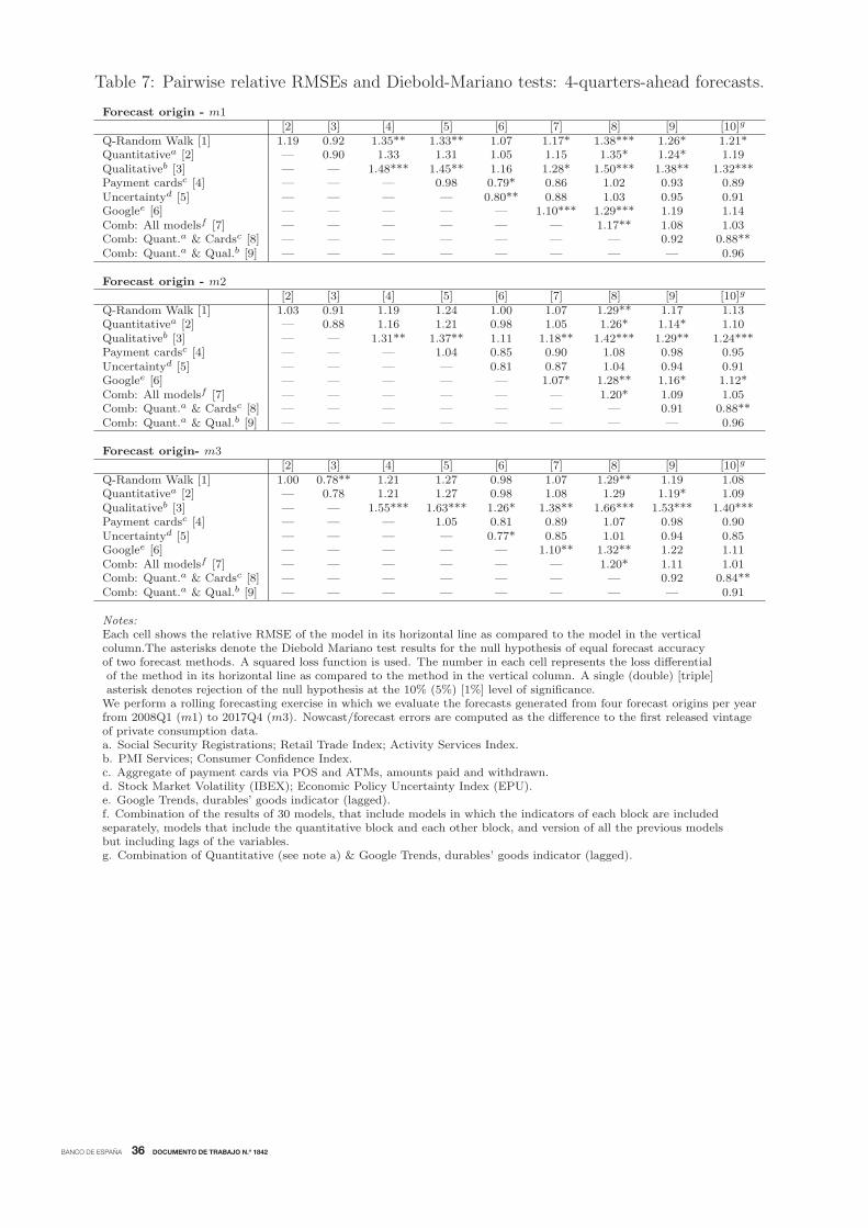
BANCO DE ESPAÑA 36 DOCUMENTO DE TRABAJO N.º 1842
Table 7: Pairwise relative RMSEs and Diebold-Mariano tests: 4-quarters-ahead forecasts.
Forecast origin - m1[2] [3] [4] [5] [6] [7] [8] [9] [10]g
Q-Random Walk [1] 1.19 0.92 1.35** 1.33** 1.07 1.17* 1.38*** 1.26* 1.21*Quantitativea [2] — 0.90 1.33 1.31 1.05 1.15 1.35* 1.24* 1.19Qualitativeb [3] — — 1.48*** 1.45** 1.16 1.28* 1.50*** 1.38** 1.32***Payment cardsc [4] — — — 0.98 0.79* 0.86 1.02 0.93 0.89Uncertaintyd [5] — — — — 0.80** 0.88 1.03 0.95 0.91Googlee [6] — — — — — 1.10*** 1.29*** 1.19 1.14Comb: All modelsf [7] — — — — — — 1.17** 1.08 1.03Comb: Quant.a & Cardsc [8] — — — — — — — 0.92 0.88**Comb: Quant.a & Qual.b [9] — — — — — — — — 0.96
Forecast origin - m2[2] [3] [4] [5] [6] [7] [8] [9] [10]g
Q-Random Walk [1] 1.03 0.91 1.19 1.24 1.00 1.07 1.29** 1.17 1.13Quantitativea [2] — 0.88 1.16 1.21 0.98 1.05 1.26* 1.14* 1.10Qualitativeb [3] — — 1.31** 1.37** 1.11 1.18** 1.42*** 1.29** 1.24***Payment cardsc [4] — — — 1.04 0.85 0.90 1.08 0.98 0.95Uncertaintyd [5] — — — — 0.81 0.87 1.04 0.94 0.91Googlee [6] — — — — — 1.07* 1.28** 1.16* 1.12*Comb: All modelsf [7] — — — — — — 1.20* 1.09 1.05Comb: Quant.a & Cardsc [8] — — — — — — — 0.91 0.88**Comb: Quant.a & Qual.b [9] — — — — — — — — 0.96
Forecast origin- m3[2] [3] [4] [5] [6] [7] [8] [9] [10]g
Q-Random Walk [1] 1.00 0.78** 1.21 1.27 0.98 1.07 1.29** 1.19 1.08Quantitativea [2] — 0.78 1.21 1.27 0.98 1.08 1.29 1.19* 1.09Qualitativeb [3] — — 1.55*** 1.63*** 1.26* 1.38** 1.66*** 1.53*** 1.40***Payment cardsc [4] — — — 1.05 0.81 0.89 1.07 0.98 0.90Uncertaintyd [5] — — — — 0.77* 0.85 1.01 0.94 0.85Googlee [6] — — — — — 1.10** 1.32** 1.22 1.11Comb: All modelsf [7] — — — — — — 1.20* 1.11 1.01Comb: Quant.a & Cardsc [8] — — — — — — — 0.92 0.84**Comb: Quant.a & Qual.b [9] — — — — — — — — 0.91
Notes:Each cell shows the relative RMSE of the model in its horizontal line as compared to the model in the verticalcolumn.The asterisks denote the Diebold Mariano test results for the null hypothesis of equal forecast accuracyof two forecast methods. A squared loss function is used. The number in each cell represents the loss differentialof the method in its horizontal line as compared to the method in the vertical column. A single (double) [triple]asterisk denotes rejection of the null hypothesis at the 10% (5%) [1%] level of significance.We perform a rolling forecasting exercise in which we evaluate the forecasts generated from four forecast origins per yearfrom 2008Q1 (m1) to 2017Q4 (m3). Nowcast/forecast errors are computed as the difference to the first released vintageof private consumption data.a. Social Security Registrations; Retail Trade Index; Activity Services Index.b. PMI Services; Consumer Confidence Index.c. Aggregate of payment cards via POS and ATMs, amounts paid and withdrawn.d. Stock Market Volatility (IBEX); Economic Policy Uncertainty Index (EPU).e. Google Trends, durables’ goods indicator (lagged).f. Combination of the results of 30 models, that include models in which the indicators of each block are includedseparately, models that include the quantitative block and each other block, and version of all the previous modelsbut including lags of the variables.g. Combination of Quantitative (see note a) & Google Trends, durables’ goods indicator (lagged).

BANCO DE ESPAÑA 37 DOCUMENTO DE TRABAJO N.º 1842
Table 8: Pesaran-Timmermann statistic of directional accuracy:a sign of private consumptiongrowth rate.
Models including indicators of only one group
Nowcast 1-q-ahead 4-q-aheadm1 m2 m3 m1 m2 m3 m1 m2 m3
Quarterly Random Walk 0.70** 0.80*** 0.80*** 0.64 0.69** 0.69** 0.50 0.56 0.56Quantitative (“hard”) indicators b 0.78*** 0.78*** 0.73*** 0.77*** 0.82*** 0.77*** 0.64*** 0.69*** 0.67***Qualitative (“soft”) indicators c 0.78*** 0.85*** 0.83*** 0.69** 0.79*** 0.77*** 0.50 0.61 0.53Payment cards (amounts,am)d 0.78*** 0.78*** 0.80*** 0.74*** 0.79*** 0.85*** 0.56 0.58 0.61Payment cards (numbers)d 0.75*** 0.75*** 0.75*** 0.72** 0.69** 0.77*** 0.50 0.69** 0.67**Uncertainty indicators e 0.73*** 0.78*** 0.78*** 0.67** 0.72*** 0.69** 0.50 0.56 0.56Google: aggregate of all indicators 0.40 0.80*** 0.80*** 0.26 0.51 0.41 0.25 0.28 0.44Google: durable goods (lagged) 0.73*** 0.73*** 0.73*** 0.69** 0.72*** 0.72*** 0.53 0.58 0.58
Models including indicators from different groups
Nowcast 1-q-ahead 4-q-aheadm1 m2 m3 m1 m2 m3 m1 m2 m3
Quantitative & Qualitative 0.78*** 0.78*** 0.78*** 0.77*** 0.87*** 0.85*** 0.64*** 0.67*** 0.67***Quantitative & Payment cards (am)d 0.78*** 0.83*** 0.78*** 0.74*** 0.77*** 0.77*** 0.61** 0.67*** 0.61**Quantitative & Uncertaintye 0.75*** 0.73*** 0.75*** 0.79*** 0.74*** 0.74*** 0.56 0.61 0.61Quantitative & Google (aggregate) 0.78*** 0.78*** 0.70*** 0.74*** 0.77*** 0.82*** 0.58 0.58 0.64**Quantitative & Google (durables) 0.78*** 0.78*** 0.78*** 0.77*** 0.82*** 0.79*** 0.64** 0.61 0.61*
Combination of modelsNowcast 1-q-ahead 4-q-ahead
m1 m2 m3 m1 m2 m3 m1 m2 m3
All models f 0.88*** 0.83*** 0.78*** 0.74*** 0.85*** 0.85*** 0.56 0.58 0.67***Hard & Payment cards (am)d 0.83*** 0.78*** 0.78*** 0.85*** 0.87*** 0.85*** 0.61* 0.69*** 0.69***Hard, Payment cards (am)d & Soft 0.83*** 0.85*** 0.78*** 0.74*** 0.82*** 0.87*** 0.53 0.61* 0.67**Hard & Soft 0.83*** 0.80*** 0.80*** 0.74*** 0.79*** 0.82*** 0.50 0.64** 0.58Hard & Google (durables) 0.78*** 0.78*** 0.75*** 0.77*** 0.77*** 0.79*** 0.56 0.58* 0.61**
Notes:The asterisks denote the PT test results for the null hypothesis. A single (double)[triple] asterisk denotes rejection of the null hypothesis at the 10% (5%) [1%] level of significance.a. Forecasts generated recursively over the moving window 2008Q1 (m1) to 2017Q4 (m3).b. Social Security Registrations; Retail Trade Index; Activity Services Index.c. PMI Services; Consumer Confidence Index.d. Aggregate of payment cards via POS and ATMs, amounts paid and withdrawn.e. Stock Market Volatility (IBEX); Economic Policy Uncertainty Index (EPU).f. Combination of the results of 30 models, that include models in which the indicators of each block are includedseparately, models that include the quantitative block and each other block, and version of all the previous modelsbut including lags of the variables.

BANCO DE ESPAÑA 38 DOCUMENTO DE TRABAJO N.º 1842
Table 9: Pesaran-Timmermann statistic of directional accuracy:a acceleration/decelerationof private consumption growth rate.
Models including indicators of only one group
Nowcast 1-q-ahead 4-q-aheadm1 m2 m3 m1 m2 m3 m1 m2 m3
Quarterly Random Walk 0.00 0.00 0.00 0.00 0.00 0.00 0.00 0.00 0.00Quantitative (“hard”) indicators b 0.55 0.73*** 0.73*** 0.54 0.54 0.62** 0.56 0.53 0.53Qualitative (“soft”) indicators c 0.48 0.55 0.55 0.49 0.54 0.56 0.64** 0.47 0.50Credit cards: POS+ATM, amounts 0.55 0.63* 0.65** 0.59 0.67** 0.64** 0.53 0.50 0.50Credit cards: POS+ATM, numbers 0.55 0.53 0.53 0.54 0.51 0.56 0.64** 0.61* 0.61*Uncertainty indicators d 0.50 0.38 0.48 0.38 0.44 0.46 0.53 0.50 0.47Google: aggregate of all indicators 0.53 0.55 0.55 0.59* 0.59* 0.56 0.53 0.44 0.50Google: durable goods (lagged) 0.48 0.53 0.53 0.46 0.46 0.49 0.64** 0.67** 0.67**
Models including indicators from different groups
Nowcast 1-q-ahead 4-q-aheadm1 m2 m3 m1 m2 m3 m1 m2 m3
Quantitative & Qualitative 0.63* 0.68*** 0.63** 0.51 0.56 0.64** 0.64* 0.64* 0.64*Quantitative & POS+ATM amounts 0.58 0.68*** 0.68*** 0.51 0.49 0.59* 0.64** 0.69*** 0.67**Quantitative & Uncertainty 0.45 0.68** 0.70*** 0.59* 0.56 0.62* 0.44 0.53 0.56Quantitative & Google (aggregate) 0.65** 0.68** 0.60* 0.46 0.56 0.59 0.69*** 0.67** 0.67**Quantitative & Google (durables) 0.48 0.65** 0.65** 0.59* 0.59* 0.62** 0.50 0.53 0.53
Combination of modelsNowcast 1-q-ahead 4-q-ahead
m1 m2 m3 m1 m2 m3 m1 m2 m3All models e 0.60 0.68*** 0.65** 0.59* 0.62** 0.64** 0.61* 0.58 0.56Hard & POS+ATM amounts 0.50 0.78*** 0.78*** 0.56 0.64** 0.59 0.58 0.53 0.53Hard, POS+ATM amounts & Soft 0.65** 0.60* 0.73*** 0.62* 0.62* 0.69*** 0.58 0.58 0.39Hard & Soft 0.58 0.63* 0.63** 0.54 0.59 0.67** 0.53 0.53 0.36Hard & Google (durables) 0.60* 0.65** 0.68*** 0.54 0.59* 0.62** 0.67** 0.58 0.58
Notes:The asterisks denote the PT test results for the null hypothesis. A single (double)[triple] asterisk denotes rejection of the null hypothesis at the 10% (5%) [1%] level of significance.a. Forecasts generated recursively over the moving window 2008Q1 (m1) to 2017Q4 (m3).b. Social Security Registrations; Retail Trade Index; Activity Services Index.c. PMI Services; Consumer Confidence Index.d. Aggregate of payment cards via POS and ATMs, amounts paid and withdrawn.e. Stock Market Volatility (IBEX); Economic Policy Uncertainty Index (EPU).f. Combination of the results of 30 models, that include models in which the indicators of each block are includedseparately, models that include the quantitative block and each other block, and version of all the previous modelsbut including lags of the variables.

BANCO DE ESPAÑA 39 DOCUMENTO DE TRABAJO N.º 1842
Figure 3: Intuitive vision of nowcast/forecast behavior from the crisis to the recovery (2008-2010): illustration based on the model with only quantitative indicators.
2008Q1 2008Q2 2008Q3
-3.0
-2.5
-2.0
-1.5
-1.0
-0.5
0.0
0.5
1.0
1.5
2.0
2005q1 2006q1 2007q1 2008q1 2009q1 2010q1 2011q1 2012q1 2013q1 2014q1
m1m2m3
-3.0
-2.5
-2.0
-1.5
-1.0
-0.5
0.0
0.5
1.0
1.5
2.0
2005q1 2006q1 2007q1 2008q1 2009q1 2010q1 2011q1 2012q1 2013q1 2014q1
m1m2m3
-3.0
-2.5
-2.0
-1.5
-1.0
-0.5
0.0
0.5
1.0
1.5
2.0
2005q1 2006q1 2007q1 2008q1 2009q1 2010q1 2011q1 2012q1 2013q1 2014q1
m1m2m3
2008Q4 2009Q1 2009Q2
-3.0
-2.5
-2.0
-1.5
-1.0
-0.5
0.0
0.5
1.0
1.5
2.0
2005q1 2006q1 2007q1 2008q1 2009q1 2010q1 2011q1 2012q1 2013q1 2014q1
m1m2m3
-3.0
-2.5
-2.0
-1.5
-1.0
-0.5
0.0
0.5
1.0
1.5
2.0
2005q1 2006q1 2007q1 2008q1 2009q1 2010q1 2011q1 2012q1 2013q1 2014q1
m1m2m3
-3.0
-2.5
-2.0
-1.5
-1.0
-0.5
0.0
0.5
1.0
1.5
2.0
2005q1 2006q1 2007q1 2008q1 2009q1 2010q1 2011q1 2012q1 2013q1 2014q1
m1m2m3
2009Q3 2009Q4 2010Q1
-3.0
-2.5
-2.0
-1.5
-1.0
-0.5
0.0
0.5
1.0
1.5
2.0
2005q1 2006q1 2007q1 2008q1 2009q1 2010q1 2011q1 2012q1 2013q1 2014q1
m1m2m3
-3.0
-2.5
-2.0
-1.5
-1.0
-0.5
0.0
0.5
1.0
1.5
2.0
2005q1 2006q1 2007q1 2008q1 2009q1 2010q1 2011q1 2012q1 2013q1 2014q1
m1m2m3
-3.0
-2.5
-2.0
-1.5
-1.0
-0.5
0.0
0.5
1.0
1.5
2.0
2005q1 2006q1 2007q1 2008q1 2009q1 2010q1 2011q1 2012q1 2013q1 2014q1
m1m2m3
2010Q2 2010Q3 2010Q4
-3.0
-2.5
-2.0
-1.5
-1.0
-0.5
0.0
0.5
1.0
1.5
2.0
2005q1 2006q1 2007q1 2008q1 2009q1 2010q1 2011q1 2012q1 2013q1 2014q1
m1m2m3
-3.0
-2.5
-2.0
-1.5
-1.0
-0.5
0.0
0.5
1.0
1.5
2.0
2005q1 2006q1 2007q1 2008q1 2009q1 2010q1 2011q1 2012q1 2013q1 2014q1
m1m2m3
-3.0
-2.5
-2.0
-1.5
-1.0
-0.5
0.0
0.5
1.0
1.5
2.0
2005q1 2006q1 2007q1 2008q1 2009q1 2010q1 2011q1 2012q1 2013q1 2014q1
m1m2m3
Notes: (i) Nowcasts/forecasts from origins m1, m2 and m3 in the quarter marked at the top of each pannel; (ii) The
dotted line denotes the 2018Q1 vintage of data, while the empty circles refer to the first released quarterly figure;
(iii) the filled-in dot denotes the available quarterly figure at m2 of each quarter.

BANCO DE ESPAÑA 40 DOCUMENTO DE TRABAJO N.º 1842
Figure 4: Intuitive vision of nowcast/forecast behavior from the crisis to the recovery (2011-2013): illustration based on the model with only quantitative indicators.
2011Q1 2011Q2 2011Q3
-3.0
-2.5
-2.0
-1.5
-1.0
-0.5
0.0
0.5
1.0
1.5
2.0
2005q1 2006q1 2007q1 2008q1 2009q1 2010q1 2011q1 2012q1 2013q1 2014q1
m1m2m3
-3.0
-2.5
-2.0
-1.5
-1.0
-0.5
0.0
0.5
1.0
1.5
2.0
2005q1 2006q1 2007q1 2008q1 2009q1 2010q1 2011q1 2012q1 2013q1 2014q1
m1m2m3
-3.0
-2.5
-2.0
-1.5
-1.0
-0.5
0.0
0.5
1.0
1.5
2.0
2005q1 2006q1 2007q1 2008q1 2009q1 2010q1 2011q1 2012q1 2013q1 2014q1
m1m2m3
2011Q4 2012Q1 2012Q2
-3.0
-2.5
-2.0
-1.5
-1.0
-0.5
0.0
0.5
1.0
1.5
2.0
2005q1 2006q1 2007q1 2008q1 2009q1 2010q1 2011q1 2012q1 2013q1 2014q1
m1m2m3
-3.0
-2.5
-2.0
-1.5
-1.0
-0.5
0.0
0.5
1.0
1.5
2.0
2005q1 2006q1 2007q1 2008q1 2009q1 2010q1 2011q1 2012q1 2013q1 2014q1
m1m2m3
-3.0
-2.5
-2.0
-1.5
-1.0
-0.5
0.0
0.5
1.0
1.5
2.0
2005q1 2006q1 2007q1 2008q1 2009q1 2010q1 2011q1 2012q1 2013q1 2014q1
m1m2m3
2012Q3 2012Q4 2013Q1
-3.0
-2.5
-2.0
-1.5
-1.0
-0.5
0.0
0.5
1.0
1.5
2.0
2005q1 2006q1 2007q1 2008q1 2009q1 2010q1 2011q1 2012q1 2013q1 2014q1
m1m2m3
-3.0
-2.5
-2.0
-1.5
-1.0
-0.5
0.0
0.5
1.0
1.5
2.0
2005q1 2006q1 2007q1 2008q1 2009q1 2010q1 2011q1 2012q1 2013q1 2014q1
m1m2m3
-3.0
-2.5
-2.0
-1.5
-1.0
-0.5
0.0
0.5
1.0
1.5
2.0
2005q1 2006q1 2007q1 2008q1 2009q1 2010q1 2011q1 2012q1 2013q1 2014q1
m1m2m3
2013Q2 2013Q3 2013Q4
-3.0
-2.5
-2.0
-1.5
-1.0
-0.5
0.0
0.5
1.0
1.5
2.0
2005q1 2006q1 2007q1 2008q1 2009q1 2010q1 2011q1 2012q1 2013q1 2014q1
m1m2m3
-3.0
-2.5
-2.0
-1.5
-1.0
-0.5
0.0
0.5
1.0
1.5
2.0
2005q1 2006q1 2007q1 2008q1 2009q1 2010q1 2011q1 2012q1 2013q1 2014q1
m1m2m3
-3.0
-2.5
-2.0
-1.5
-1.0
-0.5
0.0
0.5
1.0
1.5
2.0
2005q1 2006q1 2007q1 2008q1 2009q1 2010q1 2011q1 2012q1 2013q1 2014q1
m1m2m3
Notes: (i) Nowcasts/forecasts from origins m1, m2 and m3 in the quarter marked at the top of each pannel; (ii) The
dotted line denotes the 2018Q1 vintage of data, while the empty circles refer to the first released quarterly figure;
(iii) the filled-in dot denotes the available quarterly figure at m2 of each quarter.

BANCO DE ESPAÑA 41 DOCUMENTO DE TRABAJO N.º 1842
Figure 5: Root Mean Squared statistics of selected models by forecast origin and forecasthorizon.
0.4
0.5
0.6
0.7
0.8
0.9
1.0
1.1
1.2
1.3
Now
cast
1-q-
ah
2-q-
ah
3-q-
ah
4-q-
ah
Now
cast
1-q-
ah
2-q-
ah
3-q-
ah
4-q-
ah
Now
cast
1-q-
ah
2-q-
ah
3-q-
ah
4-q-
ah
Random walkModel with quantitative indicators (b)Combination of quantitative- and payment cards-only models (c)Combination of 30 models (d)
1st month of the quarter (m1) 2nd month of the quarter (m2) 3rd month of the quarter (m3)
Notes:
a. Forecasts generated recursively over the moving window 2008Q1 (m1) to 2017Q4 (m3). Forecast errors computed
from first vintage of released, private consumption data.
b. Model with quantitative indicators: ocial Security Registrations; Retail Trade Index; Activity Services Index.
c. Combination of quantitative-only (see footnote a) and payment cards-only (POS and ATM amounts) models.
d. Combination of the results of 30 models, that include models in which the indicators of each block are included
separately, models that include the quantitative block and each other block, and version of all the previous models
but including lags of the variables.

BANCO DE ESPAÑA 42 DOCUMENTO DE TRABAJO N.º 1842
Figure 6: Ratio of RMSEs of errors computed for two sub-samples over RMSEs computedusing the whole sample.
“Bad times”: sample 2008-2012 “Good times”: sample 2013-2017
0.00
0.25
0.50
0.75
1.00
1.25
1.50
Randomwalk
Hard(b)
Soft (c) Paymentcards(d)
Uncertainty(e)
Google(f)
Comb:all models
(g)
Comb: Hard+ Cards
(h)
m1 m2 m3
0.00
0.25
0.50
0.75
1.00
1.25
1.50
Randomwalk
Hard(b)
Soft (c) Paymentcards(d)
Uncertainty(e)
Google(f)
Comb:all models
(g)
Comb: Hard+ Cards
(h)m1 m2 m3
Notes:
a. Forecasts generated recursively over the moving window 2008Q1 (m1) to 2017Q4 (m3). Forecast errors computed from first
vintage of released private consumption data.
b. Model with quantitative indicators: Social Security Registrations; Retail Trade Index; Activity Services Index.
c. Model with qualitative indicators: PMI Services; Consumer Confidence Index.
d. Model with payment card data (aggregate of POS and ATMs amounts).
e. Model with uncertainty indicators: Stock Market Volatility (IBEX); Economic Policy Uncertainty Index (EPU).
f. Model with Google-Trends indicators: searches of durable goods, with one lag.
g. Combination of the results of 30 models, that include models in which the indicators of each block are included separately,
models that include the quantitative block and each other block, and version of all the previous models but including lags of
the variables.
h. Combination of quantitative-only (footnote b) and payment cards-only (footnote d) models.

BANCO DE ESPAÑA 43 DOCUMENTO DE TRABAJO N.º 1842
A Additional tables
Table A.1: Relative RMSE statistics: ratio of each model to the quarterly random walk.Nowcast/forecast errors computed as the difference to the 2018Q1 vintage of private con-sumption data.a
Models including indicators of only one group
Nowcast 1-q-ahead 4-q-aheadm1 m2 m3 m1 m2 m3 m1 m2 m3
Quantitative (“hard”) indicators b 0.71 * 0.78 ** 0.72 ** 0.85 0.83 0.74 0.90 0.90 0.93Qualitative (“soft”) indicators c 0.99 1.02 1.02 1.17 1.05 1.05 1.05 1.08 1.23Payment cards (amounts,am)d 0.75 * 0.90 0.94 0.76 * 0.83 0.76 * 0.70 ** 0.81 0.84Payment cards (munbers)d 1.06 1.29 * 1.27 0.98 1.00 0.98 0.72 ** 0.82 0.80 *Uncertainty indicators d 1.05 1.11 1.12 1.09 1.04 1.04 0.90 0.95 0.98Google: aggregate of all indicators 0.98 1.15 1.15 0.92 0.98 0.98 0.68 ** 0.77 * 0.77 *Google: durable goods (lagged) 1.02 1.10 1.10 1.05 1.02 1.02 0.81 * 0.89 0.89
Models including indicators from different groups
Nowcast 1-q-ahead 4-q-aheadm1 m2 m3 m1 m2 m3 m1 m2 m3
Quantitative & Qualitative 0.68 * 0.80 * 0.75 ** 0.78 0.80 0.72 * 0.73 ** 0.77 * 0.76 **Quantitative & Payment cards (am)d 0.78 0.83 0.85 0.79 0.81 0.75 0.77 ** 0.81 * 0.84Quantitative & Uncertainty 0.84 0.94 0.86 0.80 0.87 0.87 0.67 ** 0.75 * 0.75 *Quantitative & Google (aggregate) 0.80 0.87 0.88 0.84 0.88 0.78 0.69 ** 0.76 * 0.77 *Quantitative & Google (durables) 0.80 0.90 0.83 0.80 0.87 0.84 0.67 ** 0.73 ** 0.73 **
Combination of modelsNowcast 1-q-ahead 4-q-ahead
m1 m2 m3 m1 m2 m3 m1 m2 m3All models e 0.66 ** 0.79 * 0.76 * 0.77 * 0.78 * 0.69 ** 0.68 ** 0.74 ** 0.74 **Hard & Payment cards (am)d 0.56 ** 0.76 * 0.72 ** 0.66 ** 0.73 ** 0.59 *** 0.73 ** 0.80 * 0.81 *Hard, Payment cards (am)d & Soft 0.63 ** 0.80 0.77 * 0.78 * 0.79 * 0.67 ** 0.77 ** 0.84 0.88Hard & Soft 0.66 ** 0.80 0.76 * 0.86 0.82 0.72 ** 0.85 0.89 0.95Hard & Google (durables) 0.74 * 0.88 0.82 0.85 0.86 0.78 * 0.78 * 0.85 0.84
Notes:The asterisks denote the Diebold Mariano test results for the null hypothesis of equal forecast accuracy of two forecastmethods. A squared loss function is used. The number in each cell represents the loss differential of the method in itshorizontal line as compared to the quarterly random walk alternative. A single (double) [triple] asterisk denotes rejectionof the null hypothesis at the 10% (5%) [1%] level of significance.a. Nowcast/forecast errors computed as the difference to the 2018Q1 vintage of private consumption data. Forecastsgenerated recursively over the moving window 2008Q1 (m1) to 2017Q4 (m3).b. Social Security Registrations; Retail Trade Index; Activity Services Index.c. PMI Services; Consumer Confidence Index.d. Aggregate of payment cards via POS and ATMs.e. Stock Market Volatility (IBEX); Economic Policy Uncertainty Index (EPU).f. Combination of the results of 30 models, that include models in which the indicators of each block are includedseparately, models that include the quantitative block and each other block, and version of all the previous modelsbut including lags of the variables.

BANCO DE ESPAÑA 44 DOCUMENTO DE TRABAJO N.º 1842
Table A.2: Pairwise relative RMSEs and Diebold-Mariano tests: nowcasts. Nowcast errorsare computed as the difference to the 2018Q1 vintage of private consumption data.
Nowcast origin - m1[2] [3] [4] [5] [6] [7] [8] [9] [10]g
Q-Random Walk [1] 1.19 1.01 1.33* 0.94 0.95 0.98 1.52** 1.78** 1.58**Quantitativea [2] — 0.71* 0.94 0.67** 0.67** 0.69** 1.07 1.26 1.11Qualitativeb [3] — — 1.32*** 0.94 0.94 0.97 1.50** 1.76*** 1.56***Payment cardsc [4] — — — 0.71*** 0.71** 0.74** 1.14 1.33* 1.18Uncertaintyd [5] — — — — 1.00 1.04 1.61*** 1.88*** 1.67***Googlee [6] — — — — — 1.04 1.60*** 1.87*** 1.66***Comb: All modelsf [7] — — — — — — 1.55*** 1.81*** 1.60***Comb: Quant.a & Cardsc [8] — — — — — — — 1.17 1.04Comb: Quant.a & Qual.b [9] — — — — — — — — 0.89
Nowcast origin - m2[2] [3] [4] [5] [6] [7] [8] [9] [10]g
Q-Random Walk [1] 1.29** 0.98 1.11 0.77* 0.90 0.91 1.26* 1.31* 1.25Quantitativea [2] — 0.76 0.87 0.60*** 0.70* 0.71* 0.98 1.02 0.97Qualitativeb [3] — — 1.14 0.79** 0.92 0.93 1.29* 1.34* 1.28**Payment cardsc [4] — — — 0.69*** 0.81* 0.82 1.14 1.18 1.12Uncertaintyd [5] — — — — 1.17 1.17 1.64*** 1.70*** 1.61***Googlee [6] — — — — — 1.01 1.40** 1.46** 1.38**Comb: All modelsf [7] — — — — — — 1.39** 1.45** 1.37**Comb: Quant.a & Cardsc [8] — — — — — — — 1.04 0.99Comb: Quant.a & Qual.b [9] — — — — — — — — 0.95
Nowcast origin- m3[2] [3] [4] [5] [6] [7] [8] [9] [10]g
Q-Random Walk [1] 1.40** 0.98 1.06 0.79* 0.89 0.91 1.32* 1.38** 1.30*Quantitativea [2] — 0.70 0.76 0.57*** 0.64** 0.65* 0.94 0.99 0.93Qualitativeb [3] — — 1.08 0.81* 0.91 0.92 1.34* 1.41* 1.33**Payment cardsc [4] — — — 0.74** 0.84 0.85 1.24* 1.30** 1.23**Uncertaintyd [5] — — — — 1.13 1.15 1.67*** 1.75*** 1.65***Googlee [6] — — — — — 1.02 1.48*** 1.55** 1.46**Comb: All modelsf [7] — — — — — — 1.46*** 1.53** 1.44**Comb: Quant.a & Cardsc [8] — — — — — — — 1.05 0.99Comb: Quant.a & Qual.b [9] — — — — — — — — 0.94
Notes:Each cell shows the relative RMSE of the model in its horizontal line as compared to the model in the verticalcolumn.The asterisks denote the Diebold Mariano test results for the null hypothesis of equal forecast accuracyof two forecast methods. A squared loss function is used. The number in each cell represents the loss differentialof the method in its horizontal line as compared to the method in the vertical column. A single (double) [triple]asterisk denotes rejection of the null hypothesis at the 10% (5%) [1%] level of significance.We perform a rolling forecasting exercise in which we evaluate the forecasts generated from four forecast origins per yearfrom 2008Q1 (m1) to 2017Q4 (m3). Nowcast/forecast errors are computed as the difference to the first released vintageof private consumption data.a. Social Security Registrations; Retail Trade Index; Activity Services Index.b. PMI Services; Consumer Confidence Index.c. Aggregate of payment cards via POS and ATMs, amounts paid and withdrawn.d. Stock Market Volatility (IBEX); Economic Policy Uncertainty Index (EPU).e. Google Trends, durables’ goods indicator (lagged).f. Combination of the results of 30 models, that include models in which the indicators of each block are includedseparately, models that include the quantitative block and each other block, and version of all the previous modelsbut including lags of the variables.g. Combination of Quantitative (see note a) & Google Trends, durables’ goods indicator (lagged).

BANCO DE ESPAÑA 45 DOCUMENTO DE TRABAJO N.º 1842
Table A.3: Pairwise relative RMSEs and Diebold-Mariano tests: 1-quarters-ahead forecasts.Forecast errors are computed as the difference to the 2018Q1 vintage of private consumptiondata.
Forecast origin - m1[2] [3] [4] [5] [6] [7] [8] [9] [10]g
Q-Random Walk [1] 1.34** 0.85 1.31* 1.02 0.92 0.95 1.30* 1.50** 1.28*Quantitativea [2] — 0.72** 1.11 0.87 0.78** 0.81* 1.10 1.27** 1.08Qualitativeb [3] — — 1.54*** 1.20** 1.08 1.12 1.52*** 1.76*** 1.50***Payment cardsc [4] — — — 0.78*** 0.70*** 0.73*** 0.99 1.15 0.98Uncertaintyd [5] — — — — 0.90 0.93 1.27*** 1.47*** 1.25**Googlee [6] — — — — — 1.04* 1.41*** 1.63*** 1.39***Comb: All modelsf [7] — — — — — — 1.36*** 1.58*** 1.34***Comb: Quant.a & Cardsc [8] — — — — — — — 1.16*** 0.99Comb: Quant.a & Qual.b [9] — — — — — — — — 0.85***
Forecast origin - m2[2] [3] [4] [5] [6] [7] [8] [9] [10]g
Q-Random Walk [1] 1.20 0.95 1.21 1.00 0.96 0.98 1.28* 1.36** 1.27*Quantitativea [2] — 0.79* 1.01 0.83 0.80* 0.82* 1.07 1.14 1.06Qualitativeb [3] — — 1.27** 1.05 1.01 1.03 1.35** 1.43*** 1.34***Payment cardsc [4] — — — 0.83* 0.80** 0.81* 1.06 1.13* 1.05Uncertaintyd [5] — — — — 0.96 0.98 1.28** 1.36** 1.27**Googlee [6] — — — — — 1.02 1.33*** 1.42*** 1.32***Comb: All modelsf [7] — — — — — — 1.31** 1.39*** 1.30***Comb: Quant.a & Cardsc [8] — — — — — — — 1.06 0.99Comb: Quant.a & Qual.b [9] — — — — — — — — 0.93
Forecast origin- m3[2] [3] [4] [5] [6] [7] [8] [9] [10]g
Q-Random Walk [1] 1.34 0.95 1.31* 1.03 0.96 0.98 1.46** 1.71*** 1.50***Quantitativea [2] — 0.71* 0.98 0.76 0.71* 0.73* 1.08 1.27* 1.11Qualitativeb [3] — — 1.38*** 1.08 1.01 1.03 1.53*** 1.80*** 1.58***Payment cardsc [4] — — — 0.78* 0.73** 0.75** 1.11 1.30* 1.14Uncertaintyd [5] — — — — 0.93 0.96 1.42** 1.66*** 1.46**Googlee [6] — — — — — 1.02 1.52*** 1.78*** 1.56***Comb: All modelsf [7] — — — — — — 1.48*** 1.74*** 1.52***Comb: Quant.a & Cardsc [8] — — — — — — — 1.17** 1.03Comb: Quant.a & Qual.b [9] — — — — — — — — 0.88
Notes:Each cell shows the relative RMSE of the model in its horizontal line as compared to the model in the verticalcolumn.The asterisks denote the Diebold Mariano test results for the null hypothesis of equal forecast accuracyof two forecast methods. A squared loss function is used. The number in each cell represents the loss differentialof the method in its horizontal line as compared to the method in the vertical column. A single (double) [triple]asterisk denotes rejection of the null hypothesis at the 10% (5%) [1%] level of significance.We perform a rolling forecasting exercise in which we evaluate the forecasts generated from four forecast origins per yearfrom 2008Q1 (m1) to 2017Q4 (m3). Nowcast/forecast errors are computed as the difference to the first released vintageof private consumption data.a. Social Security Registrations; Retail Trade Index; Activity Services Index.b. PMI Services; Consumer Confidence Index.c. Aggregate of payment cards via POS and ATMs, amounts paid and withdrawn.d. Stock Market Volatility (IBEX); Economic Policy Uncertainty Index (EPU).e. Google Trends, durables’ goods indicator (lagged).f. Combination of the results of 30 models, that include models in which the indicators of each block are includedseparately, models that include the quantitative block and each other block, and version of all the previous modelsbut including lags of the variables.g. Combination of Quantitative (see note a) & Google Trends, durables’ goods indicator (lagged).

BANCO DE ESPAÑA 46 DOCUMENTO DE TRABAJO N.º 1842
Table A.4: Pairwise relative RMSEs and Diebold-Mariano tests: 4-quarters-ahead forecasts.Forecast errors are computed as the difference to the 2018Q1 vintage of private consumptiondata.
Forecast origin - m1[2] [3] [4] [5] [6] [7] [8] [9] [10]g
Q-Random Walk [1] 1.19 0.95 1.42** 1.39** 1.11 1.24* 1.48*** 1.38** 1.30**Quantitativea [2] — 0.86 1.28 1.25 1.00 1.11 1.33 1.24* 1.16Qualitativeb [3] — — 1.49*** 1.46*** 1.17 1.29* 1.55*** 1.44** 1.36***Payment cardsc [4] — — — 0.98 0.78** 0.87 1.04 0.97 0.91Uncertaintyd [5] — — — — 0.80*** 0.89 1.06 0.99 0.93Googlee [6] — — — — — 1.11*** 1.33*** 1.24* 1.16*Comb: All modelsf [7] — — — — — — 1.20** 1.11 1.05Comb: Quant.a & Cardsc [8] — — — — — — — 0.93 0.88**Comb: Quant.a & Qual.b [9] — — — — — — — — 0.94
Forecast origin - m2[2] [3] [4] [5] [6] [7] [8] [9] [10]g
Q-Random Walk [1] 1.11 0.93 1.23 1.22 1.05 1.13 1.36** 1.25* 1.19Quantitativea [2] — 0.83 1.11 1.09 0.94 1.01 1.22 1.12 1.07Qualitativeb [3] — — 1.33*** 1.31** 1.13 1.22** 1.46*** 1.35*** 1.28***Payment cardsc [4] — — — 0.99 0.85* 0.91 1.10 1.01 0.96Uncertaintyd [5] — — — — 0.86 0.93 1.12 1.03 0.98Googlee [6] — — — — — 1.07 1.30*** 1.19* 1.13*Comb: All modelsf [7] — — — — — — 1.20** 1.11 1.05Comb: Quant.a & Cardsc [8] — — — — — — — 0.92 0.87**Comb: Quant.a & Qual.b [9] — — — — — — — — 0.95
Forecast origin - m3[2] [3] [4] [5] [6] [7] [8] [9] [10]g
Q-Random Walk [1] 1.07 0.82 1.19 1.26* 1.02 1.13 1.35** 1.24* 1.14Quantitativea [2] — 0.76 1.11 1.17 0.95 1.05 1.26 1.15 1.06Qualitativeb [3] — — 1.46** 1.54*** 1.25* 1.38** 1.65*** 1.52** 1.40***Payment cardsc [4] — — — 1.05 0.85 0.94 1.13 1.04 0.96Uncertaintyd [5] — — — — 0.81** 0.90 1.08 0.99 0.91Googlee [6] — — — — — 1.10** 1.32*** 1.22 1.12Comb: All modelsf [7] — — — — — — 1.20** 1.10 1.02Comb: Quant.a & Cardsc [8] — — — — — — — 0.92 0.85**Comb: Quant.a & Qual.b [9] — — — — — — — — 0.92
Notes:Each cell shows the relative RMSE of the model in its horizontal line as compared to the model in the verticalcolumn.The asterisks denote the Diebold Mariano test results for the null hypothesis of equal forecast accuracyof two forecast methods. A squared loss function is used. The number in each cell represents the loss differentialof the method in its horizontal line as compared to the method in the vertical column. A single (double) [triple]asterisk denotes rejection of the null hypothesis at the 10% (5%) [1%] level of significance.We perform a rolling forecasting exercise in which we evaluate the forecasts generated from four forecast origins per yearfrom 2008Q1 (m1) to 2017Q4 (m3). Nowcast/forecast errors are computed as the difference to the first released vintageof private consumption data.a. Social Security Registrations; Retail Trade Index; Activity Services Index.b. PMI Services; Consumer Confidence Index.c. Aggregate of payment cards via POS and ATMs, amounts paid and withdrawn.d. Stock Market Volatility (IBEX); Economic Policy Uncertainty Index (EPU).e. Google Trends, durables’ goods indicator (lagged).f. Combination of the results of 30 models, that include models in which the indicators of each block are includedseparately, models that include the quantitative block and each other block, and version of all the previous modelsbut including lags of the variables.g. Combination of Quantitative (see note a) & Google Trends, durables’ goods indicator (lagged).

BANCO DE ESPAÑA 47 DOCUMENTO DE TRABAJO N.º 1842
Table A.5: Pesaran-Timmermann statistic of directional accuracy: sign of private consump-tion growth rate. Nowcast/forecast errors computed as the difference to the 2018Q1 vintageof private consumption data.a
Models including indicators of only one group
Nowcast 1-q-ahead 4-q-aheadm1 m2 m3 m1 m2 m3 m1 m2 m3
Quarterly Random Walk 0.80*** 0.90*** 0.90*** 0.69*** 0.79*** 0.79*** 0.58 0.58 0.58Quantitative (“hard”) indicators b 0.88*** 0.83*** 0.83*** 0.82*** 0.82*** 0.87*** 0.72*** 0.72*** 0.75***Qualitative (“soft”) indicators c 0.68** 0.75*** 0.78*** 0.64* 0.69** 0.67** 0.58 0.53 0.56Payment cards (amounts,am)d 0.78*** 0.78*** 0.80*** 0.74*** 0.74*** 0.79*** 0.64* 0.61 0.64*Payment cards (numbers)d 0.75*** 0.75*** 0.80*** 0.62 0.69** 0.82*** 0.58 0.72*** 0.69**Uncertainty indicators e 0.73*** 0.78*** 0.78*** 0.62* 0.67** 0.69*** 0.53 0.53 0.58Google: aggregate of all indicators 0.30 0.80*** 0.80*** 0.15 0.41 0.36 0.28 0.19 0.36Google: durable goods (lagged) 0.73*** 0.78*** 0.78*** 0.59 0.72*** 0.72*** 0.56 0.56 0.56
Models including indicators from different groups
Nowcast 1-q-ahead 4-q-aheadm1 m2 m3 m1 m2 m3 m1 m2 m3
Quantitative & Qualitative 0.88*** 0.88*** 0.88*** 0.82*** 0.82*** 0.85*** 0.72*** 0.69*** 0.69***Quantitative & Payment cards (am)d 0.83*** 0.88*** 0.83*** 0.79*** 0.82*** 0.82*** 0.69*** 0.69*** 0.69***Quantitative & Uncertainty 0.70*** 0.78*** 0.80*** 0.85*** 0.79*** 0.79*** 0.53 0.58 0.56Quantitative & Google (aggregate) 0.78*** 0.78*** 0.75*** 0.69*** 0.67** 0.77*** 0.72*** 0.61 0.78***Quantitative & Google (durables) 0.83*** 0.83*** 0.83*** 0.77*** 0.77*** 0.79*** 0.72*** 0.64* 0.69***
Combination of modelsNowcast 1-q-ahead 4-q-ahead
m1 m2 m3 m1 m2 m3 m1 m2 m3
All models f 0.83*** 0.85*** 0.88*** 0.74*** 0.82*** 0.85*** 0.64** 0.58 0.69***Hard & Payment cards (am)d 0.83*** 0.83*** 0.83*** 0.85*** 0.82*** 0.85*** 0.64** 0.67** 0.72***Hard, Payment cards (am)d & Soft 0.78*** 0.80*** 0.83*** 0.74*** 0.77*** 0.82*** 0.56 0.58 0.64**Hard & Soft 0.78*** 0.85*** 0.85*** 0.69*** 0.79*** 0.77*** 0.58 0.61* 0.56Hard & Google (durables) 0.83*** 0.88*** 0.85*** 0.77*** 0.77*** 0.79*** 0.64** 0.67** 0.69***
Notes:The asterisks denote the PT test results for the null hypothesis. A single (double)[triple] asterisk denotes rejection of the null hypothesis at the 10% (5%) [1%] level of significance.a. Forecasts generated recursively over the moving window 2008Q1 (m1) to 2017Q4 (m3).b. Social Security Registrations; Retail Trade Index; Activity Services Index.c. PMI Services; Consumer Confidence Index.d. Aggregate of payment cards via POS and ATMs, amounts paid and withdrawn.e. Stock Market Volatility (IBEX); Economic Policy Uncertainty Index (EPU).f. Combination of the results of 30 models, that include models in which the indicators of each block are includedseparately, models that include the quantitative block and each other block, and version of all the previous modelsbut including lags of the variables.

BANCO DE ESPAÑA 48 DOCUMENTO DE TRABAJO N.º 1842
Table A.6: Pesaran-Timmermann statistic of directional accuracy: acceleration/decelerationof private consumption. Nowcast/forecast errors computed as the difference to the 2018Q1vintage of private consumption data.a
Models including indicators of only one group
Nowcast 1-q-ahead 4-q-aheadm1 m2 m3 m1 m2 m3 m1 m2 m3
Quarterly Random Walk 0.00 0.00 0.00 0.00 0.00 0.00 0.00 0.00 0.00Quantitative (“hard”) indicators b 0.55 0.73*** 0.73*** 0.54 0.54 0.62** 0.56 0.53 0.53Qualitative (“soft”) indicators c 0.48 0.55 0.55 0.49 0.54 0.56 0.64** 0.47 0.50Credit cards: POS+ATM, amounts 0.55 0.63* 0.65** 0.59 0.67** 0.64** 0.53 0.50 0.50Credit cards: POS+ATM, numbers 0.55 0.53 0.53 0.54 0.51 0.56 0.64** 0.61* 0.61*Uncertainty indicators d 0.50 0.38 0.48 0.38 0.44 0.46 0.53 0.50 0.47Google: aggregate of all indicators 0.53 0.55 0.55 0.59* 0.59* 0.56 0.53 0.44 0.50Google: durable goods (lagged) 0.48 0.53 0.53 0.46 0.46 0.49 0.64** 0.67** 0.67**
Models including indicators from different groups
Nowcast 1-q-ahead 4-q-aheadm1 m2 m3 m1 m2 m3 m1 m2 m3
Quantitative & Qualitative 0.63* 0.68*** 0.63** 0.51 0.56 0.64** 0.64* 0.64* 0.64*Quantitative & POS+ATM amounts 0.58 0.68*** 0.68*** 0.51 0.49 0.59* 0.64** 0.69*** 0.67**Quantitative & Uncertainty 0.45 0.68** 0.70*** 0.59* 0.56 0.62* 0.44 0.53 0.56Quantitative & Google (aggregate) 0.65** 0.68** 0.60* 0.46 0.56 0.59 0.69*** 0.67** 0.67**Quantitative & Google (durables) 0.48 0.65** 0.65** 0.59* 0.59* 0.62** 0.50 0.53 0.53
Combination of modelsNowcast 1-q-ahead 4-q-ahead
m1 m2 m3 m1 m2 m3 m1 m2 m3All models e 0.60 0.68*** 0.65** 0.59* 0.62** 0.64** 0.61* 0.58 0.56Hard & POS+ATM amounts 0.50 0.78*** 0.78*** 0.56 0.64** 0.59 0.58 0.53 0.53Hard, POS+ATM amounts & Soft 0.65** 0.60* 0.73*** 0.62* 0.62* 0.69*** 0.58 0.58 0.39Hard & Soft 0.58 0.63* 0.63** 0.54 0.59 0.67** 0.53 0.53 0.36Hard & Google (durables) 0.60* 0.65** 0.68*** 0.54 0.59* 0.62** 0.67** 0.58 0.58
Notes:The asterisks denote the PT test results for the null hypothesis. A single (double)[triple] asterisk denotes rejection of the null hypothesis at the 10% (5%) [1%] level of significance.a. Forecasts generated recursively over the moving window 2008Q1 (m1) to 2017Q4 (m3).b. Social Security Registrations; Retail Trade Index; Activity Services Index.c. PMI Services; Consumer Confidence Index.d. Aggregate of payment cards via POS and ATMs, amounts paid and withdrawn.e. Stock Market Volatility (IBEX); Economic Policy Uncertainty Index (EPU).f. Combination of the results of 30 models, that include models in which the indicators of each block are includedseparately, models that include the quantitative block and each other block, and version of all the previous modelsbut including lags of the variables.

BANCO DE ESPAÑA PUBLICATIONS
WORKING PAPERS
1801 OLYMPIA BOVER, LAURA HOSPIDO and ERNESTO VILLANUEVA: The impact of high school financial education on
financial knowledge and choices: evidence from a randomized trial in Spain.
1802 IGNACIO HERNANDO, IRENE PABLOS, DANIEL SANTABÁRBARA and JAVIER VALLÉS: Private Saving. New Cross-
Country Evidence Based on Bayesian Techniques.
1803 PABLO AGUILAR and JESÚS VÁZQUEZ: Term structure and real-time learning.
1804 MORITZ A. ROTH: International co-movements in recessions.
1805 ANGELA ABBATE and DOMINIK THALER: Monetary policy and the asset risk-taking channel.
1806 PABLO MARTÍN-ACEÑA: Money in Spain. New historical statistics. 1830-1998.
1807 GUILHERME BANDEIRA: Fiscal transfers in a monetary union with sovereign risk.
1808 MIGUEL GARCÍA-POSADA GÓMEZ: Credit constraints, fi rm investment and growth: evidence from survey data.
1809 LAURA ALFARO, MANUEL GARCÍA-SANTANA and ENRIQUE MORAL-BENITO: On the direct and indirect real
effects of credit supply shocks.
1810 ROBERTO RAMOS and CARLOS SANZ: Backing the incumbent in diffi cult times: the electoral impact of wildfi res.
1811 GABRIEL JIMÉNEZ, ENRIQUE MORAL-BENITO and RAQUEL VEGAS: Bank lending standards over the cycle:
the role of fi rms’ productivity and credit risk.
1812 JUAN S. MORA-SANGUINETTI and ROK SPRUK: Industry vs services: do enforcement institutions matter for
specialization patterns? Disaggregated evidence from Spain.
1813 JAMES CLOYNE, CLODOMIRO FERREIRA and PAOLO SURICO: Monetary policy when households have debt: new
evidence on the transmission mechanism.
1814 DMITRI KIRPICHEV and ENRIQUE MORAL-BENITO: The costs of trade protectionism: evidence from Spanish fi rms
and non-tariff measures.
1815 ISABEL ARGIMÓN, CLEMENS BONNER, RICARDO CORREA, PATTY DUIJM, JON FROST, JAKOB DE HAAN,
LEO DE HAAN and VIKTORS STEBUNOVS: Financial institutions’ business models and the global transmission of
monetary policy.
1816 JOSE ASTURIAS, MANUEL GARCÍA-SANTANA and ROBERTO RAMOS: Competition and the welfare gains from
transportation infrastructure: evidence from the Golden Quadrilateral of India.
1817 SANDRA GARCÍA-URIBE: Multidimensional media slant: complementarities in news reporting by US newspapers .
1818 PILAR CUADRADO, AITOR LACUESTA, MARÍA DE LOS LLANOS MATEA and F. JAVIER PALENCIA-GONZÁLEZ:
Price strategies of independent and branded dealers in retail gas market. The case of a contract reform in Spain.
1819 ALBERTO FUERTES, RICARDO GIMENO and JOSÉ MANUEL MARQUÉS: Extraction of infl ation expectations from
fi nancial instruments in Latin America.
1820 MARIO ALLOZA, PABLO BURRIEL and JAVIER J. PÉREZ: Fiscal policies in the euro area: revisiting the size of spillovers.
1821 MARTA MARTÍNEZ-MATUTE and ALBERTO URTASUN: Uncertainty, fi rm heterogeneity and labour adjustments.
Evidence from European countries.
1822 GABRIELE FIORENTINI, ALESSANDRO GALESI, GABRIEL PÉREZ-QUIRÓS and ENRIQUE SENTANA: The rise and fall
of the natural interest rate.
1823 ALBERTO MARTÍN, ENRIQUE MORAL-BENITO and TOM SCHMITZ: The fi nancial transmission of housing bubbles:
evidence from Spain.
1824 DOMINIK THALER: Sovereign default, domestic banks and exclusion from international capital markets.
1825 JORGE E. GALÁN and JAVIER MENCÍA: Empirical assessment of alternative structural methods for identifying cyclical
systemic risk in Europe.
1826 ROBERTO BLANCO and NOELIA JIMÉNEZ: Credit allocation along the business cycle: evidence from the latest boom
bust credit cycle in Spain.
1827 ISABEL ARGIMÓN: The relevance of currency-denomination for the cross-border effects of monetary policy.
1828 SANDRA GARCÍA-URIBE: The effects of tax changes on economic activity: a narrative approach to frequent anticipations.
1829 MATÍAS CABRERA, GERALD P. DWYER and MARÍA J. NIETO: The G-20 regulatory agenda and bank risk.
1830 JACOPO TIMINI and MARINA CONESA: Chinese exports and non-tariff measures: testing for heterogeneous effects at the
product level.
1831 JAVIER ANDRÉS, JOSÉ E. BOSCÁ, JAVIER FERRI and CRISTINA FUENTES-ALBERO: Households’ balance sheets and
the effect of fi scal policy.

1832 ÓSCAR ARCE, MIGUEL GARCÍA-POSADA, SERGIO MAYORDOMO and STEVEN ONGENA: Adapting lending policies
when negative interest rates hit banks’ profi ts.
1833 VICENTE SALAS, LUCIO SAN JUAN and JAVIER VALLÉS: Corporate cost and profi t shares in the euro area and the US:
the same story?
1834 MARTÍN GONZÁLEZ-EIRAS and CARLOS SANZ: Women’s representation in politics: voter bias, party bias, and electoral
systems.
1835 MÓNICA CORREA-LÓPEZ and BEATRIZ DE BLAS: Faraway, so close! Technology diffusion and fi rm heterogeneity in the
medium term cycle of advanced economies.
1836 JACOPO TIMINI: The margins of trade: market entry and sector spillovers, the case of Italy (1862-1913).
1837 HENRIQUE S. BASSO and OMAR RACHEDI: The young, the old, and the government: demographics and fi scal
multipliers.
1838 PAU ROLDÁN and SONIA GILBUKH: Firm dynamics and pricing under customer capital accumulation.
1839 GUILHERME BANDEIRA, JORDI CABALLÉ and EUGENIA VELLA: Should I stay or should I go? Austerity,
unemployment and migration.
1840 ALESSIO MORO and OMAR RACHEDI: The changing structure of government consumption spending.
1841 GERGELY GANICS, ATSUSHI INOUE and BARBARA ROSSI: Confi dence intervals for bias and size distortion in IV
and local projections — IV models.
1842 MARÍA GIL, JAVIER J. PÉREZ, A. JESÚS SÁNCHEZ and ALBERTO URTASUN: Nowcasting private consumption:
traditional indicators, uncertainty measures, credit cards and some internet data.
Unidad de Servicios AuxiliaresAlcalá, 48 - 28014 Madrid
E-mail: [email protected]