MIT-CTP/4864, PUPT 2515

NPTFit: A code package for Non-Poissonian Template Fitting

Siddharth Mishra-Sharma,1, ∗ Nicholas L. Rodd,2, † and Benjamin R. Safdi2, ‡

1Department of Physics, Princeton University, Princeton, NJ 085442Center for Theoretical Physics, Massachusetts Institute of Technology, Cambridge, MA 02139

(Dated: June 7, 2017)

We present NPTFit, an open-source code package, written in python and cython, for performingnon-Poissonian template fits (NPTFs). The NPTF is a recently-developed statistical procedure forcharacterizing the contribution of unresolved point sources (PSs) to astrophysical data sets. TheNPTF was first applied to Fermi gamma-ray data to give evidence that the excess of ∼GeV gamma-rays observed in the inner regions of the Milky Way likely arises from a population of sub-thresholdpoint sources, and the NPTF has since found additional applications studying sub-threshold extra-galactic sources at high Galactic latitudes. The NPTF generalizes traditional astrophysical templatefits to allow for the ability to search for populations of unresolved PSs that may follow a given spa-tial distribution. NPTFit builds upon the framework of the fluctuation analyses developed in X-rayastronomy, and thus likely has applications beyond those demonstrated with gamma-ray data. TheNPTFit package utilizes novel computational methods to perform the NPTF efficiently. The code isavailable at https://github.com/bsafdi/NPTFit and up-to-date and extensive documentation maybe found at http://nptfit.readthedocs.io.

I. INTRODUCTION

Astrophysical point sources (PSs), which are definedas sources with angular extent smaller than the resolu-tion of the detector, play an important role in virtuallyevery analysis utilizing images of the cosmos. It is use-ful to distinguish between resolved and unresolved PSs;the former may be detected individually at high signif-icance, while members of the latter population are bydefinition too dim to be detected individually. However,unresolved PSs – due to their potentially large numberdensity – can be a leading and sometimes pesky source offlux across wavelengths. Recently, a novel analysis tech-nique called the non-Poissonian template fit (NPTF) hasbeen developed for characterizing populations of unre-solved PSs at fluxes below the detection threshold forfinding individually-significant sources [1, 2]. The tech-nique expands upon the traditional fluctuation analysistechnique (see, for example, [3, 4]), which analyzes theaggregate photon-count statistics of a data set to charac-terize the contribution from unresolved PSs, by addition-ally incorporating spatial information both for the distri-bution of unresolved PSs and for the potential sources ofnon-PS emission. In this work, we present a code packagecalled NPTFit for numerically implementing the NPTF inpython and cython.

The most up-to-date version of the open-source pack-age NPTFit may be found at

https://github.com/bsafdi/NPTFit

and the latest documentation at

http://nptfit.readthedocs.io.

∗ smsharma@princeton.edu† nrodd@mit.edu‡ bsafdi@mit.edu

In addition, the version used in this paper has beenarchived at

https://zenodo.org/record/380469#.WN_pSFPyvMV.

The NPTF generalizes traditional astrophysical tem-plate fits. Template fitting is useful for pixelated datasets consisting of some number of photon counts np ineach pixel p, and it typically proceeds as follows. Givena set of model parameters θ, the mean number of pre-dicted photon counts µp(θ) in the pixel p may be com-

puted. More specifically, µp(θ) =∑` T

(S)p,` (θ), where `

is an index of the set of templates T(S)p,` , whose normal-

izations and spatial morphologies may depend on the pa-rameters θ. These templates may, for example, trace thegas-distribution or other extended structures that are ex-pected to produce photon counts. Then, the probabilityto detect np photons in the pixel p is simply given bythe Poisson distribution with mean µp(θ). By taking aproduct of the probabilities over all pixels, it is straight-forward to write down a likelihood function as a functionof θ.

The NPTF modifies this procedure by allowing for non-Poissonian photon-count statistics in the individual pix-els. That is, unresolved PS populations are allowed tobe distributed according to spatial templates, but in thepresence of unresolved PSs the photon-count statistics inindividual pixels, as parameterized by θ, no longer fol-low Poisson distributions. This is heuristically becausewe now have to ask two questions in each pixel: first,what is the probability, given the model parameters θthat now also characterize the intrinsic source-count dis-tribution of the PS population, that there are PSs withinthe pixel p, then second, given that PS population, whatis the probability to observe np photons?

It is important to distinguish between resolved and un-resolved PSs. Once a PS is resolved – that is once its lo-cation and flux is known – that PS may be accounted for

arX

iv:1

612.

0317

3v2

[as

tro-

ph.H

E]

6 J

un 2

017

2

by its own Poissonian template. Unresolved PSs are dif-ferent because their locations and fluxes are not known.When we characterize unresolved PSs with the NPFT, wecharacterize the entire population of unresolved sources,following a given spatial distribution, based on how thatpopulation modifies the photon-count statistics.

The NPTF has played an important role recently inaddressing various problems in gamma-ray astroparticlephysics with data collected by the Fermi-LAT gamma-ray telescope.1 The NPTF was developed to address theexcess of gamma rays observed by Fermi at ∼GeV en-ergies originating from the inner regions of the MilkyWay [5–18]. The GeV excess, as it is commonly referredto, has received a significant amount of attention due tothe possibility that the excess emission arises from darkmatter (DM) annihilation. However, it is well known thatunresolved PSs may complicate searches for annihilatingDM in the Inner Galaxy region due to, for example, theexpected population of dim pulsars [12, 19–26]. In [2](see also [27]) it was shown, using the NPTF, that in-deed the photon-count statistics of the data prefer a PSover a smooth DM interpretation of the GeV excess. Thesame conclusion was also reached by [28] using an unre-lated method that analyzes the statistics of peaks in thewavelet transformation of the Fermi data.

In the case of the GeV excess, there are multiple PSpopulations that may contribute to the observed gamma-ray flux and complicate the search for DM annihilation.These include isotropically distributed PSs of extragalac-tic origin, PSs distributed along the disk of the MilkyWay such as supernova remnants and pulsars, and apotential spherical population of PSs such as millisec-ond pulsars. Additionally, there are various identifiedPSs that contribute significantly to the flux as well asa variety of smooth emission mechanisms such as gas-correlated emission from pion decay and bremsstrahlung.The power of the NPTF is that these different sourceclasses may be given separate degrees of freedom and con-strained by incorporating the spatial morphology of theirvarious contributions along with the difference in photon-count statistics between smooth emission and emissionfrom unresolved PSs. Although the origin of the GeVexcess is still not completely settled, as even if the ex-cess arises from PSs as the NPTF suggests the sourceclass of the PSs remains a mystery at present, the NPTFhas emerged as a powerful tool for analyzing populationsof dim PSs in complicated data sets with characteristicspatial morphology.

The NPTF and related techniques utilizing photon-count statistics have also been used recently to studythe contribution of various source classes to the extra-galactic gamma-ray background (EGB) [4, 29–32].2 Inthese works it was shown that unresolved blazars would

1 http://fermi.gsfc.nasa.gov/2 The complementary analysis strategy of probabilistic catalogues

has also been applied to this problem [33].

predominantly show up as PS populations under theNPTF, while other source classes such as star-forminggalaxies would show up predominantly as smooth emis-sion. For example, in [32] it was shown using the NPTFthat blazars likely account for the majority of the EGBfrom ∼2 GeV to ∼2 TeV. These results set strong con-straints on the flux from more diffuse sources, such asstar-forming galaxies, which has significant implicationsfor, among other problems, the interpretation of the high-energy astrophysical neutrinos observed by IceCube [34–37] (see, for example, [38, 39]). This is because certainsources that contribute gamma-ray flux at Fermi ener-gies, such as star forming galaxies and various types ofactive galactic nuclei, may also contribute neutrino fluxobservable by IceCube.

The NPTF originates from the older fluctuation analy-sis technique, which is sometimes referred to as the P (D)analysis. This technique has been used extensively tostudy the flux of unresolved X-ray sources [3, 40–43]. Inthese early works, the photon-count probability distribu-tion function (PDF) was computed numerically for dif-ferent PS source-count distributions using Monte Carlo(MC) techniques. The fluctuation analysis was first ap-plied to gamma-ray data in [4],3 and in that work the au-thors developed a semi-analytic technique utilizing prob-ability generating functions for calculating the photon-count PDF. The code package NPTFit presented in thiswork uses this formalism for efficiently calculating thephoton-count PDF. The specific form of the likelihoodfunction for the NPTF, while reviewed in this work, wasfirst presented in [2]. The works [2, 27, 32] utilized anearly version of NPTFit to perform their numerical anal-yses.

The NPTFit code package has a python interface,though the likelihood evaluation is efficiently imple-mented in cython [46]. The user-friendly interface allowsfor an arbitrary number of PS and smooth templates.The PS templates are characterized by pixel-dependent

source-count distributions dNp/dF = T(PS)p dN/dF ,

where T(PS)p is the spatial template tracking the distribu-

tion of point sources on the sky and dN/dF is the pixel-independent source-count distribution. The distributiondNp/dF quantifies the number of sources dNp that con-tributes flux between F and F + dF in the pixel p. ThedN/dF are parameterized as multiply broken power-laws,with an arbitrary number of breaks. The code is able toaccount for both an arbitrary exposure map (account-ing for the pointing strategy of an instrument) as well asan arbitrary point spread function (PSF, accounting forthe instrument’s finite angular resolution) in translatingbetween flux F and counts S.NPTFit has a built-in interface with MultiNest [47, 48],

which efficiently implements nested sampling of the pos-

3 The fluctuation analysis has more recently been applied to bothgamma-ray [44] and neutrino [45] datasets.

3

terior distribution and Bayesian evidence for the user-specified model, given the specified data and instru-ment response function, in the Bayesian framework [49–51]. The interface handles the Message Passing Interface(MPI), so that inference may be performed efficiently us-ing parallel computing. A basic analysis package is pro-vided in order to facilitate easy extraction of the mostrelevant data from the posterior distribution and quickplotting of the MultiNest output. The preferred formatof the data for NPTFit is HEALPix [52] (a nested equal-area pixilation scheme of the sky), although the the codeis also able to handle non-HEALPix data arrays. Notethat the code package may also be used to simply ex-tract the NPTF likelihood function so that NPTFit maybe interfaced with any numerical package for Bayesian orfrequentist inference.

A large set of example Jupyter [53] notebooks andpython files are provided to illustrate the code. The ex-amples utilize 413 weeks of processed Fermi Pass 8 datain the UltracleanVeto event class collected between Au-gust 4, 2008 and July 7, 2016 in the energy range from 2to 20 GeV. We restrict this dataset to the top quartile asgraded by PSF reconstruction and further apply the stan-dard quality cuts DATA_QUAL==1 && LAT_CONFIG==1, aswell as restricting the zenith angle to be less than 90◦.This data is made available in the code release. More-over, the example notebooks illustrate many of the mainresults in [2, 27, 32].

In addition to the above, the base NPTFit code makesuse of the python packages corner [54], matplotlib [55],mpmath [56], GSL [57] and numpy [58].

The rest of this paper is organized as follows. Section IIoutlines in more detail the framework of the NPTF. Sec-tion III highlights the key classes and features in the NPT-Fit code package and usage instructions. In Sec. IV wepresent an example of how to perform an NPTF scan us-ing NPTFit, looking at the Galactic Center with Fermidata to reproduce aspects of the main results of [2]. Weconclude in Sec. V. Appendices A, B, and C describe fur-ther details behind the mathematical framework of theNPTF.

II. THE NON-POISSONIAN TEMPLATE FIT

In this section we review the NPTF, which was firstpresented in [2] and described in more detail in [27, 32](see also [1, 4, 29, 31]). The NPTF is used to fit a modelM with parameters θ to a data set d consisting of countsnp in each pixel p. The likelihood function for the NPTFis then simply

p(d|θ,M) =∏p

p(p)np

(θ) , (1)

where p(p)np (θ) gives the probability of drawing np counts

in the given pixel p, as a function of the parameters θ.The main computational challange, of course, is in com-puting these probabilities.

It is useful to divide the model parameters into twodifferent categories: the first category describes smoothtemplates, while the second category describes PS tem-plates. We describe each category in turn, starting withthe smooth templates.

For most applications, the data has the interpretationof being a two-dimensional pixelated map consisting ofan integer number of counts in each pixel. The smoothtemplates may be used to predict the mean number ofcounts µp(θ) in each pixel p:

µp(θ) =∑`

µp,`(θ) . (2)

Above, ` is an index over templates and µp,`(θ) denotesthe mean contribution of the `th template to pixel pfor parameters θ. In principle, θ may describe boththe spatial morphology as well as the normalization ofthe templates. However, in the current implementationof the code, the Poissonian model parameters simplycharacterize the overall normalization of the templates:

µp,`(θ) = A`(θ)T(S)p,` . Here, A` is the normalization pa-

rameter and T(S)p,` is the `th template, which takes values

over all pixels p and is independent of the model param-eters. The superscript (S) implies that the template is acounts templates, which is to be contrasted with a fluxtemplate, for which we use the symbol (F ). The twoare related by the exposure map of the instrument Ep:

T(S)p = EpT

(F )p . In the case where we only have smooth,

Poissonian templates, the probabilities are then given bythe Poisson distribution:

p(p)np

(θ) =µnpp (θ)

np!e−µp(θ) . (3)

In the presence of unresolved PS templates, the prob-

abilities p(p)np (θ) are no longer Poissonian functions of the

model parameters θ. Each PS template is characterizedby a pixel-dependent source-count distribution dNp/dF ,which describes the differential number of sources perpixel per unit flux interval. In this work, we model thesource-count distribution by a multiply broken power-law:

4

dNpdF

(F ;θ) = A(θ)T (PS)p

(FFb,1

)−n1

, F ≥ Fb,1(FFb,1

)−n2

, Fb,1 > F ≥ Fb,2(Fb,2

Fb,1

)−n2(

FFb,2

)−n3

, Fb,2 > F ≥ Fb,3(Fb,2

Fb,1

)−n2(Fb,3

Fb,2

)−n3(

FFb,3

)−n4

, Fb,3 > F ≥ Fb,4

. . . . . .[∏k−1i=1

(Fb,i+1

Fb,i

)−ni+1](

FFb,k

)−nk+1

, Fb,k > F

. (4)

Above, we have parameterized the source-count dis-tribution with an arbitrary number of breaks k, de-noted by Fb,i with i ∈ [1, 2, . . . , k], and k + 1 indices niwith i ∈ [1, 2, . . . , k + 1]. The spatial dependence of thesource-count distribution is accounted for by the overall

factor A(θ)T(PS)p , where A(θ) is the pixel-independent

normalization, which is a function of the model parame-

ters, and T(PS)p is a template describing the spatial dis-

tribution of the PSs. More precisely, the number ofsources NPS

p =∫dFdNp/dF (and the total PS flux

FPSp =

∫dFFdNp/dF ) in pixel p, for a fixed set of model

parameters θ, follows the template T(PS)p . On the other

hand, the locations of the flux breaks and the indices aretaken to be fixed between pixels.4

To summarize, a PS template described by a brokenpower-law with k breaks has 2(k + 1) model parametersdescribing the locations of the breaks, the power-law in-dices, and the overall normalization. For example, if wetake a single break then the PS model parameters may bedenoted as {A,Fb,1, n1, n2}. Additionally, a spatial tem-

plate T (PS) must be specified, which describes the dis-tribution of the number of sources (and total flux) withpixel p.

Notice that when we discussed the Poissonian tem-plates we used the counts templates T (S) and talkeddirectly in terms of counts S, while so far in our dis-cussion of the unresolved PS templates we have usedthe point source distribution template T (PS) and writ-ten the source-count distribution dN/dF in terms of fluxF . Of course as the total flux from a distribution ofpoint sources is also proportional to the template T (PS),it can be thought of as a flux template, however concep-tually it is being used to track the distribution of thesources rather than the flux they produce. For this rea-son we have chosen to distinguish the two. Moreover,in the presence of a non-trivial PSF, T (S) should alsobe smoothed by the PSF to account for the instrument

4 In principle, the breaks and indices could also vary between pix-els. However, in the current version of NPTFit, only the numberof sources (and, accordingly, the total flux) is allowed to varybetween pixels.

response function. That is, T (S) is a template for theobserved counts taking into account the details of theinstrument, while T (PS) (T (F )) is a map of the physi-cal point sources (flux), which is independent of the in-strument. In photon-counting applications, the exposuremap Ep often has units of cm2s and flux has units ofcounts cm−2s−1.

For the unresolved PS templates, we also need to con-vert the source-count distribution from flux to counts.This is done by a simple change of variables:

dNpdS

(S;θ) =1

Ep

dNpdF

(F = S/Ep;θ) , (5)

which implies that for a non-Poissonian template the

spatial dependence of dNp/dS is given by T(PS)p /Ep.

This inverse exposure scaling may seem surprising, butit is straightforward to confirm that the mean numberof counts in a given pixel,

∫dSSdNp/dS, is given by

EpT(PS)p , as expected, up to pixel independent factors.

As an important aside, the template T (S) used by thePoissonian models needs to be smoothed by the PSF.Incorporating the PSF into the unresolved PS models,on the other hand, is more complicated and is not ac-complished simply by smoothing the spatial template.

Indeed, T(PS)p should remain un-smoothed by the PSF

when used for non-Poissonian scans.In the remainder of this section we briefly overview the

mathematic framework behind the computation of the

p(p)np (θ) with NPTFit; however, details of the algorithms

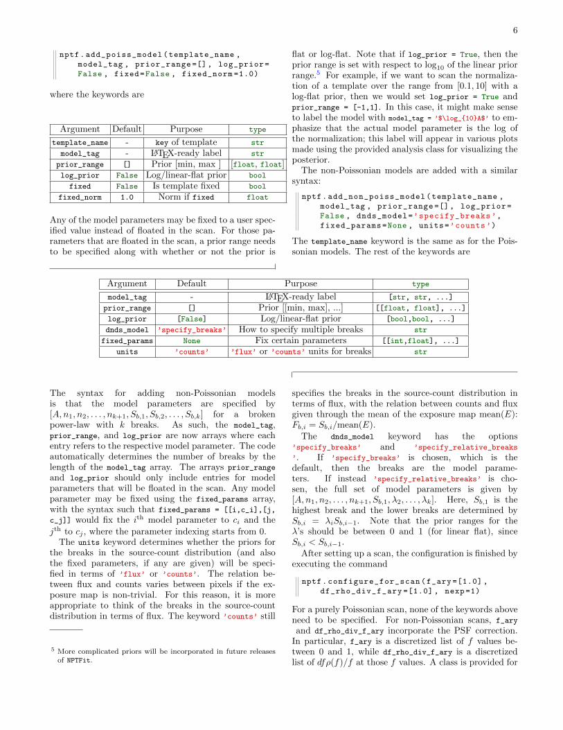
used to calculate these probabilities in practice, alongwith more in-depth explanations, are given in Apps. A, B,and C. We use the probability generating function for-malism, following [4], to calculate the probabilities. Fora discrete probability distribution pk, with k = 0, 1, 2, . . .,the generating function is defined as:

P (t) ≡∞∑k=0

pktk , (6)

from which we can recover the probabilities:

pk =1

k!

dkP (t)

dtk

∣∣∣∣t=0

. (7)

5

The key feature of generating functions exploited here isthat the generating function of a sum of two independentrandom variables is simply the product of the individualgenerating functions.

The probability generating function for the smoothtemplates, as a function of θ, is simply given by

PP(t;θ) =∏p

exp [µp(θ)(t− 1)] . (8)

The probability generating function for an unresolved PStemplate, on the other hand, takes a more complicatedform:

PNP(t;θ) =∏p

exp

[ ∞∑m=1

xp,m(θ)(tm − 1)

], (9)

where

xp,m(θ) =

∫ ∞0

dSdNpdS

(S;θ)

∫ 1

0

dfρ(f)(fS)m

m!e−fS .

(10)

Above, ρ(f) is a function that takes into account thePSF, which we describe in more detail in App. A. Inthe presence of a non-trivial PSF, the flux from a singlesource is smeared among pixels. The distribution of fluxfractions among pixels is described by the function ρ(f),where f is the flux fraction. By definition ρ(f)df equalsthe number of pixels which, on average, contain betweenf and f + df of the flux from a PS; the distribution is

normalized such that∫ 1

0dffρ(f) = 1. If the PSF is a

δ-function, then ρ(f) = δ(f − 1).Putting aside the PSF correction for the moment, the

xp,m have the interpretation of being the average numberof m-count PSs within the pixel p, given the distributiondNp(S;θ)/dS. The generating function for xm m-count

sources is simply exm(tm−1) (see [4] or App. A), whichthen leads directly to (9). The PSF correction, throughthe distribution ρ(f), incorporates the fact that PSs onlycontribute some fraction of their flux within a given pixel.

III. NPTFIT: ORIENTATION

NPTFit implements the NPTF, as described above, inpython. In this section we give a brief orientation tothe code package and its main classes. A more thoroughdescription of the code and its uses is available in theonline documentation.

class NPTFit.nptfit.NPTF

This is the main class used to set up and perform non-Poissonian and Poissonian template scans. It is initial-ized by

nptf = NPTF(tag=’Untagged ’,work_dir=None)

with keywords

Argument Default Purpose type

tag ’Untagged’ Label of scan str

work_dir None Output directory str

.

If no work_dir is specified, the code will default to thecurrent directory. This is the directory where all outputis stored. Specifying a tag will create an additional folder,with that name, within the work_dir for the output.

The data, exposure map, and templates are loaded intothe nptfit.NPTF instance after initialization (see the ex-ample in Sec. IV). The data and exposure map are loadedby

nptf.load_data(data , exposure)

Here, data and exposure are 1-D numpy arrays. The rec-ommended format for these arrays is the HEALPix format,so that all pixels are equal area, although the code is ableto handle arbitrary data and exposure arrays so long asthey are of the same length. The templates are added by

nptf.add_template(template , key ,

units=’counts ’)

Here, template is a 1-D numpy array of the same lengthas the data and exposure map, key is a string that will beused to refer to the template later on, and units specifieswhether the template is a counts template (keyword ’

counts’) or a flux template (keyword ’flux’) in unitscounts cm−2s−1. The default, if unspecified, is units =

’counts’. The template should be pre-smoothed by thePSF if it is going to be used for a Poissonian model. Ifthe template is going to be used for a non-Poissonianmodel, either choice for units is acceptable, though inthe case of ’counts’ the template should simply be theproduct of the exposure map times the flux template andnot smoothed by the PSF.

The user also has the option of loading in a mask thatreduces the region of interest (ROI) to a subset of thepixels in the data, exposure, and template arrays. Thisis done through the command

nptf.load_mask(mask)

where mask is a boolean numpy array of the same lengthas the data and exposure arrays. Pixels in mask shouldbe either True or False; by convention, pixels that areTrue will be masked, while those that are False will notbe masked. Note if performing an analysis with non-Poissonian templates, regions where the exposure map isidentically zero should be explicitly masked.

Afterwards, Poissonian and non-Poissonian modelsmay be added to the instance using the available tem-plates. An arbitrary number of Poissonian and non-Poissonian models may be added to the scan. Moreover,each non-Poissonian model may be specified in terms of amultiply broken power law with a user-specified numberof breaks, as in (4).

Poissonian models are added sequentially using thesyntax

6

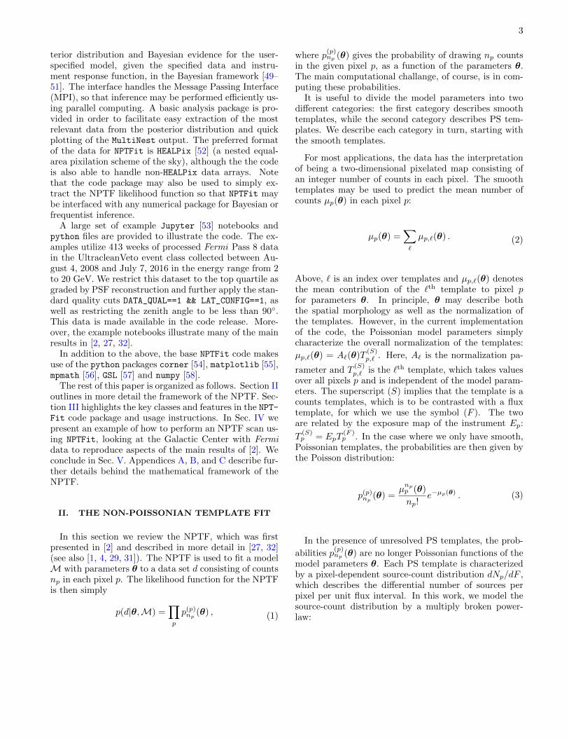
nptf.add_poiss_model(template_name ,

model_tag , prior_range =[], log_prior=

False , fixed=False , fixed_norm =1.0)

where the keywords are

Argument Default Purpose type

template_name - key of template str

model_tag - LATEX-ready label str

prior_range [] Prior [min, max ] [float, float]log_prior False Log/linear-flat prior bool

fixed False Is template fixed bool

fixed_norm 1.0 Norm if fixed float

Any of the model parameters may be fixed to a user spec-ified value instead of floated in the scan. For those pa-rameters that are floated in the scan, a prior range needsto be specified along with whether or not the prior is

flat or log-flat. Note that if log_prior = True, then theprior range is set with respect to log10 of the linear priorrange.5 For example, if we want to scan the normaliza-tion of a template over the range from [0.1, 10] with alog-flat prior, then we would set log_prior = True andprior_range = [-1,1]. In this case, it might make senseto label the model with model_tag = ’$\log_{10}A$’ to em-phasize that the actual model parameter is the log ofthe normalization; this label will appear in various plotsmade using the provided analysis class for visualizing theposterior.

The non-Poissonian models are added with a similarsyntax:

nptf.add_non_poiss_model(template_name ,

model_tag , prior_range =[], log_prior=

False , dnds_model=’specify_breaks ’,

fixed_params=None , units=’counts ’)

The template_name keyword is the same as for the Pois-sonian models. The rest of the keywords are

Argument Default Purpose type

model_tag - LATEX-ready label [str, str, ...]

prior_range [] Prior [[min, max], ...] [[float, float], ...]

log_prior [False] Log/linear-flat prior [bool,bool, ...]

dnds_model ’specify_breaks’ How to specify multiple breaks str

fixed_params None Fix certain parameters [[int,float], ...]

units ’counts’ ’flux’ or ’counts’ units for breaks str

The syntax for adding non-Poissonian modelsis that the model parameters are specified by[A,n1, n2, . . . , nk+1, Sb,1, Sb,2, . . . , Sb,k] for a brokenpower-law with k breaks. As such, the model_tag,prior_range, and log_prior are now arrays where eachentry refers to the respective model parameter. The codeautomatically determines the number of breaks by thelength of the model_tag array. The arrays prior_range

and log_prior should only include entries for modelparameters that will be floated in the scan. Any modelparameter may be fixed using the fixed_params array,with the syntax such that fixed_params = [[i,c_i],[j,

c_j]] would fix the ith model parameter to ci and the

jth to cj , where the parameter indexing starts from 0.The units keyword determines whether the priors for

the breaks in the source-count distribution (and alsothe fixed parameters, if any are given) will be speci-fied in terms of ’flux’ or ’counts’. The relation be-tween flux and counts varies between pixels if the ex-posure map is non-trivial. For this reason, it is moreappropriate to think of the breaks in the source-countdistribution in terms of flux. The keyword ’counts’ still

5 More complicated priors will be incorporated in future releasesof NPTFit.

specifies the breaks in the source-count distribution interms of flux, with the relation between counts and fluxgiven through the mean of the exposure map mean(E):Fb,i = Sb,i/mean(E).

The dnds_model keyword has the options’specify_breaks’ and ’specify_relative_breaks

’. If ’specify_breaks’ is chosen, which is thedefault, then the breaks are the model parame-ters. If instead ’specify_relative_breaks’ is cho-sen, the full set of model parameters is given by[A,n1, n2, . . . , nk+1, Sb,1, λ2, . . . , λk]. Here, Sb,1 is thehighest break and the lower breaks are determined bySb,i = λiSb,i−1. Note that the prior ranges for theλ’s should be between 0 and 1 (for linear flat), sinceSb,i < Sb,i−1.

After setting up a scan, the configuration is finished byexecuting the command

nptf.configure_for_scan(f_ary =[1.0] ,

df_rho_div_f_ary =[1.0] , nexp =1)

For a purely Poissonian scan, none of the keywords aboveneed to be specified. For non-Poissonian scans, f_ary

and df_rho_div_f_ary incorporate the PSF correction.In particular, f_ary is a discretized list of f values be-tween 0 and 1, while df_rho_div_f_ary is a discretizedlist of dfρ(f)/f at those f values. A class is provided for

7

computing these lists; it is described later in this section.If no keywords are given for these two arrays they defaultto the case of a δ-function PSF.

The keyword nexp, which defaults to 1, is related to theexposure correction in the calculation of the source-countdistribution dNp/dS from dNp/dF . In many applica-tions, it is computationally too expensive to perform themapping in (5) in each pixel. The overall pixel-dependent

normalization factor T(PS)p /Ep factorizes from many of

the internal computations, and as a result this contri-bution to the exposure correction is performed in everypixel. However, it is useful to perform the mapping fromflux to counts, which should be performed uniquely ineach pixel F = S/Ep, using the mean exposure withinsmall sub-regions. Within a given sub-region, we mapflux to counts using F = S/mean(E), where the mean istaken over all pixels in the sub-region. The number ofsub-regions is given by nexp, and all sub-regions have ap-proximately the same area. As nexp approaches the num-ber of pixels, the approximation becomes exact; however,for many applications the approximation converges for arelatively small number of exposure regions. We recom-mend verifying, in any application, that results are stableas nexp is increased.

After configuring the NPTF instance, the log-likelihoodmay be extracted, as a function of the model parameters,in addition to the prior range. The log-likelihood andprior range may then be used with any external packagefor performing Bayesian or frequentist inference. Thisis particularly useful if the user would like to combinelikelihood functions between different energy bins or oth-erwise add to the default likelihood function, for example,incorporating nuisance parameters beyond those associ-ated with individual templates. The package MultiNest,however, is already incorporated into the NPTF class and

may be run immediately after configuring the NPTF in-stance. This is done simply by executing the command

nptf.perform_scan(run_tag=None ,nlive =100)

where nlive is an integer that specifies the number of livepoints used in the sampling of the posterior distribution.MultiNest recommends an nlive ∼500-1000, though theparameter defaults to 100 if unspecified for quick testruns. Additional MultiNest arguments may be passedas a dictionary through the optional pymultinest_optionskeyword (see the online documentation for more details).The optional keyword run_tag is used to create a sub-folder for the MultiNest output with that name.

After a scan has been run (or if a scan has been runpreviously and saved), the results may be loaded throughthe command

nptf.load_scan(run_tag=None)

The MultiNest chains, which give a discretized view ofthe posterior distribution, may then be accessed through,for example, nptf.samples. An instance of the PyMulti-Nest analyzer class may be accessed through nptf.a. Asmall analysis package, described later in this section, isalso provided for performing a few common analyses.

class NPTFit.psf_correction.PSFCorrection

This is the class used to construct the arrays f_ary anddf_rho_div_f_ary for the PSF correction. An instance ofPSFCorrection is initialized through

pc_inst = PSFCorrection.PSFCorrection(

psf_dir=None , num_f_bins =10, n_psf

=50000 , n_pts_per_psf =1000, f_trunc

=0.01, nside =128, psf_sigma_deg=None ,

delay_compute=False)

with keywords

Argument Default Purpose type

psf_dir None Where PSF arrays are stored str

num_f_bins 10 Number of linear-spaced points inf_ary int

n_psf 50000 Number of MC simulations for determining df_rho_div_f_ary int

n_pts_per_psf 1000 Number of points drawn for each MC simulation int

f_trunc 0.01 Minimum f value float

nside 128 HEALPix parameter for size of map int

psf_sigma_deg None Standard deviation σ of 2-D Gaussian PSF float

delay_compute False If True, PSF not Gaussian and will be specified later bool

Note that the arrays f_ary and df_rho_div_f_ary dependboth on the PSF of the detector as well as the pixelationof the data; at present the PSFCorrection class requiresthe pixelation to be in the HEALPix pixelation.

The keyword psf_dir points to the directory where thef_ary and df_rho_div_f_ary will be stored; if unspecified,they will be stored to the current directory. The f_ary

consists of num_f_bins entries linear spaced between 0

and 1. The PSF correction involves placing many (n_psf)PSFs at random positions on the HEALPix map, drawingn_pts_per_psf points from each PSF, and then looking atthe distribution of points among pixels. The larger n_psf

and n_pts_per_psf, the more accurate the computationof df_rho_div_f_ary will be. However, the computationtime of the PSF arrays also increases as these parametersare increased.

8

By default the PSFCorrection class assumes that thePSF is a 2-D Gaussian distribution:

PSF(r) =1

2πσ2exp

[− r2

2σ2

]. (11)

Here, PSF(r) describes the spread of arriving counts withangular distance r away from the arrival direction. Theparameter psf_sigma_deg denotes σ in degrees. Upon ini-tializing PSFCorrection with psf_sigma_deg specified, theclass automatically computes the array df_rho_div_f_ary

and stores it in the psf_dir with a unique name re-lated to the keywords. If such a file already exists inthe psf_dir, then the code will simply load this file in-stead of recomputing it. After initialization, the relevantarrays may be accessed by pc_inst.f_ary and pc_inst.

df_rho_div_f_ary.The PSFCorrection class can also handle arbitrary

PSF functions. In this case, the class should be ini-tialized with delay_compute = True. Then, the usershould manually set the function pc_inst.psf_r_func

to the desired function PSF(r). This function willbe discretized with pc_inst.psf_samples points out topc_inst.sample_psf_max degrees from r = 0. Thesetwo quantities also need to be manually specified. Theuser also needs to set pc_inst.psf_tag to a string thatwill be used for saving the PSF arrays. After thesefour attributes have been set manually by the user,the PSF arrays are computed and stored by executingpc_inst.make_or_load_psf_corr().

def NPTFit.create_mask.make_mask_total

This function is used to make masks that can thenbe used to reduce the data and templates to a smallerROI when performing the scan. While these masks canalways be made by hand, this function provides a sim-ple masking interface for maps in the HEALPix format.The make_mask_total function can mask pixels by lati-tude, longitude, and radius from any point on the sphere.See the online documentation for more specific examples.

class NPTFit.dnds_analysis.Analysis

The analysis class may be used to extract useful in-formation from the results of an NPTF performed usingMultiNest. The class also has built-in plotting featuresfor making many of the most common types of visual-izations for the parameter posterior distribution. An in-stance of the analysis class can be instantiated by

an = Analysis(nptf , mask=None , pixarea

=0.)

where nptf is itself an instance of the NPTF class that al-ready has the results of a scan loaded. The keyword ar-guments mask and pixarea are optional. The user should

specify a mask if the desired ROI for the analysis is differ-ent that that used in the scan. The user should specifya pixarea if the data is not in the HEALPix format. Thecode will still assume the pixels are equal area with areapixarea, which should be specified in sr.

After initialization, the intensities of Poissonian andnon-Poissonian templates, respectively, may be extractedfrom the analysis class by the commands

an.return_intensity_arrays_poiss(comp)

and

an.return_intensity_arrays_non_poiss(

comp)

Here, comp refers to the template key used by the Poisso-nian or non-Poissonian model. The arrays returned givethe mean intensities of that model in the ROI in units ofcounts cm−2s−1, assuming the exposure map was in unitsof cm2s. The arrays computed over the full set of entriesin the discretized posterior distribution output by Multi-Nest. Thus, these intensity arrays may be interpreted asthe 1-D posteriors for the intensities. For additional key-words that may be used to customize the computation ofthe intensity arrays, see the online documentation.

The source-count distributions may also be accessedfrom the analysis class. Executing

an.return_dndf_arrays(comp , flux)

will return the discretized 1-D posterior distribution formeanROIdNp(F )/dF at flux F for the PS model withtemplate key comp. Note that the mean is computed overpixels p in the ROI.

The 1-D posterior distributions for the individualmodel parameters may be accessed by

A_poiss_post = an.

return_poiss_parameter_posteriors(

comp)

for Poissonian models, and

A_non_poiss_post , n_non_poiss_post ,

Sb_non_poiss_post = an.

return_non_poiss_parameter_posteriors(

comp)

for non-Poissonian models. Here A_poiss_post isa 1-D array of the discretized posterior distribu-tion for the Poissonian template normalizationparameter. Similarly, A_non_poiss_post is theposterior array for the non-Poissonian normaliza-tion parameter. The arrays n_non_poiss_post andSb_non_poiss_post are 2-D, where – for example –n_non_poiss_post = [n_1_array, n_2_array, ...] andn_1_array is a 1-D array for the posterior for n1.

Another useful piece of information that may be ex-tracted from the scan is the Bayesian evidence:

l_be , l_be_err = an.get_log_evidence ()

returns the log of the Bayesian evidence along with theuncertainty on this estimate based on the resolution ofthe MCMC.

9

For information on the plotting capabilities in the anal-ysis class, see the online documentation or the examplein the following section.

IV. NPTFIT: AN EXAMPLE

In this section we give an example for how to performan NPTF using NPTFit. Many more examples are avail-able in the online documentation. This particular exam-ple reproduces aspects of the main results of [2], whichfound evidence for a spherical population of unresolvedgamma-ray PSs around the Galactic Center. The exam-ple uses the processed, public Fermi data made availablewith the release of the NPTFit package. The data set con-sists of 413 weeks of Fermi Pass 8 data in the Ultraclean-Veto event class (top quartile of events as ranked by PSF)from 2 to 20 GeV. The map is binned in HEALPix withnside = 128. The data, along with the exposure mapand background templates, may be downloaded from

http://hdl.handle.net/1721.1/105492.

In the example we will perform an NPTF on the sub-region where we mask the Galactic plane at latitude |b| <2◦ and mask pixels with angular distance greater than 30◦

from the Galactic Center. We also mask identified PSsin the 3FGL PS catalog [59] at 95% containment usingthe provided PS mask, which is added to the geometricmask. We include smooth templates for diffuse gamma-ray emission in the Milky Way (using the Fermi p6v11diffuse model), isotropic emission (which can also absorbinstrumental backgrounds), and emission following theFermi bubbles, which are taken to be uniform in fluxfollowing the spatial template in [60]. We also includea dark matter template, which traces the line of sightintegral of the square of a canonical NFW density profile.

We additionally include point source (non-Poissonian)models for the DM template, as well as for a disk tem-plate which corresponds to a doubly exponential thin-disk source distribution with scale height 0.3 kpc andradius 5 kpc. The source-count distributions for theseare parameterized by singly-broken power laws, each de-scribed by four parameters {A,Fb,1, n1, n2}.

A. Setting up the scan

We begin the example by loading in the relevant mod-ules, described in the previous section, that we will needto setup, perform, and analyze the scan.

import numpy as np

# module for performing scan

from NPTFit import nptfit

# module for creating the mask

from NPTFit import create_mask as cm

# module for determining the PSF

correction

from NPTFit import psf_correction as pc

# module for analyzing the output

from NPTFit import dnds_analysis

Next, we create an instance of the NPTF class, which isused to configure and perform a scan.

n = nptfit.NPTF(tag=’GCE_Example ’)

We assume here that the supplementary Fermi data hasbeen downloaded to a directory ’fermi_data’. Then, wemay load in the data and exposure maps by

fermi_data = np.load(’fermi_data/

fermidata_counts.npy’).astype(int)

fermi_exposure = np.load(’fermi_data/

fermidata_exposure.npy’)

n.load_data(fermi_data , fermi_exposure)

Importantly, note that the exposure map has units ofcm2s. Next, we use the create_mask class to generate ourROI mask, which consists of both the geometric mask andthe PS mask loaded in from the ’fermi_data’ directory:

pscmask=np.array(np.load(’fermi_data/

fermidata_pscmask.npy’), dtype=bool)

mask = cm.make_mask_total(band_mask =

True , band_mask_range = 2, mask_ring =

True , inner = 0, outer = 30,

custom_mask = pscmask)

n.load_mask(mask)

The templates may also be loaded in from this directory,

dif = np.load(’fermi_data/template_dif.

npy’)

iso = np.load(’fermi_data/template_iso.

npy’)

bub = np.load(’fermi_data/template_bub.

npy’)

gce = np.load(’fermi_data/template_gce.

npy’)

dsk = np.load(’fermi_data/template_dsk.

npy’)

These templates are counts map (i.e. flux maps times theexposure map) that have been pre-smoothed by the PSF(except for the disk-correlated template labeled dsk). Wethen add them to our NPTF instance with appropriatelychosen keywords:

n.add_template(dif , ’dif’)

n.add_template(iso , ’iso’)

n.add_template(bub , ’bub’)

n.add_template(gce , ’gce’)

n.add_template(dsk , ’dsk’)

# remove the exposure correction for PS

templates

rescale = fermi_exposure/np.mean(

fermi_exposure)

n.add_template(gce/rescale , ’gce_np ’,

units=’PS’)

n.add_template(dsk/rescale , ’dsk_np ’,

units=’PS’)

Note that templates ’gce_np’ and ’dsk_np’ intendedto be used in non-Poissonian models should trace theunderlying PS distribution, without exposure correction,and are added with the keyword units=’PS’.

10

B. Adding models

Now that we have loaded in all of the external dataand templates, we can add models to our NPTF instance.First, we add in the Poissonian models,

n.add_poiss_model(’dif’, ’$A_\mathrm{dif}

$’, False , fixed=True , fixed_norm

=14.67)

n.add_poiss_model(’iso’, ’$A_\mathrm{iso}

$’, [0,2], False)

n.add_poiss_model(’gce’, ’$A_\mathrm{gce}

$’, [0,2], False)

n.add_poiss_model(’bub’, ’$A_\mathrm{bub}

$’, [0,2], False)

All Poissonian models are taken to have linear priors,with prior ranges for the normalizations between 0 and2. However, the normalization of the diffuse backgroundhas been fixed to the value 14.67, which is approximatelythe correct normalization in these units for this template,in order to provide an example of this syntax. Next, weadd in the two non-Poissonian models:

n.add_non_poiss_model(’gce_np ’, [’$A_\

mathrm{gce}^\ mathrm{ps}$’,’$n_1^\

mathrm{gce}$’,’$n_2^\ mathrm{gce}$’,’

$S_b ^{(1) , \mathrm{gce}}$’],

[[ -6 ,1] ,[2.05 ,30] ,[ -2 ,1.95] ,[0.05 ,40]] ,

[True ,False ,False ,False])

n.add_non_poiss_model(’dsk_np ’, [’$A_\

mathrm{dsk}^\ mathrm{ps}$’,’$n_1^\

mathrm{dsk}$’,’$n_2^\ mathrm{dsk}$’,’

$S_b ^{(1) , \mathrm{dsk}}$’],

[[ -6 ,1] ,[2.05 ,30] ,[ -2 ,1.95] ,[0.05 ,40]] ,

[True ,False ,False ,False])

We have added in the models for disk-correlated andNFW-correlated (line of sight integral of the the NFWdistribution squared) unresolved PS templates. Each ofthese models takes singly-broken power-law source-countdistributions. In each case, the normalization parame-ter is taken to have a log-flat prior while the indices andbreaks are taken to have linear priors. The units of thebreaks are specified in terms of counts.

C. Configure scan with PSF correction

In this energy range and with this data set, the PSFmay be modeled by a 2-D Gaussian distribution withσ = 0.1812◦. From this, we are able to construct thePSF-correction arrays:6

pc_inst = pc.PSFCorrection(psf_sigma_deg

=0.1812)

f_ary , df_rho_div_f_ary = pc_inst.f_ary ,

pc_inst.df_rho_div_f_ary

6 For an example of how to construct these arrays with a morecomplicated, non-Gaussian PSF function, see the online docu-mentation.

These arrays are then passed into the NPTF instance whenwe configure the scan:

n.configure_for_scan(f_ary ,

df_rho_div_f_ary , nexp =1)

Note that since our ROI is relatively small and the expo-sure map does not change significantly over the region,we have a single exposure region with nexp=1.

D. Performing the scan with MultiNest

We perform the scan using MultiNest with nlive=100

as an example to demonstrate the basic features and con-clusions of this analysis while being able to perform thescan in a reasonable amount of time on a single processor,although ideally nlive should be set to a higher value formore reliable results:

n.perform_scan(nlive =100)

E. Analyzing the results

Now, we are ready to analyze the results of the scan.First we load in relevant modules:

import corner

import matplotlib.pyplot as plt

and then we load in the results of the scan (configured asabove),

n.load_scan ()

The chains, giving a discretized view of the posterior dis-tribution, may be accessed simply through the attributen.samples. However, we will analyze the results by usingthe analysis class provided with NPTFit. We make aninstance of this class simply by

an = dnds_analysis.Analysis(n)

1. Make triangle plots

Triangle plots are a simple and quick way of visualizingcorrelations in the posterior distribution. Such plots maybe generated through the command

an.make_triangle ()

which leads to the plot in Fig. 1.

2. Plot source-count distributions

The source-count distributions for NFW- and disk-correlated point source models may be plotted with

11

Aiso = 0.44+0.06−0.06

0.02

0.04

0.06

0.08

Agc

e

Agce = 0.01+0.02−0.01

0.78

0.84

0.90

0.96

Ab

ub

Abub = 0.88+0.04−0.04

−3.6−3.0−2.4

Ap

sgc

e

Apsgce = −2.53+0.20

−0.30

6

12

18

24

ngc

e1

ngce1 = 18.79+7.45

−7.89

−1.6−0.8

0.0

0.8

ngc

e2

ngce2 = −1.04+0.92

−0.66

8

16

24

32

S(1

),gc

eb

S(1),gceb = 16.44+3.50

−2.75

−3.6−3.2−2.8−2.4

Ap

sd

sk

Apsdsk = −3.09+0.27

−0.31

6

12

18

24

nd

sk1

ndsk1 = 16.95+9.26

−8.50

−1.6−0.8

0.0

0.8

nd

sk2

ndsk2 = −0.90+0.86

−0.79

0.32

0.40

0.48

0.56

Aiso

20253035

S(1

),d

skb

0.02

0.04

0.06

0.08

Agce

0.78

0.84

0.90

0.96

Abub−3.6−3.0−2.4

Apsgce

6 12 18 24

ngce1

−1.6−0.8 0.

00.

8

ngce2

8 16 24 32

S(1),gceb

−3.6−3.2−2.8−2.4

Apsdsk

6 12 18 24

ndsk1

−1.6−0.8 0.

00.

8

ndsk2

20 25 30 35

S(1),dskb

S(1),dskb = 27.49+5.68

−5.10

FIG. 1. The triangle plot obtained by analyzing the results of an NPTF in the Galactic Center, showing the one and two dimen-sional posteriors of the 11 parameters floated in the fit corresponding to three Poissonian and two non-Poissonian templates.For this analysis 3FGL point sources have been masked at 95% containment. See text for details.

an.plot_source_count_median(’dsk’,smin

=0.01, smax =1000, nsteps =1000, color=’

cornflowerblue ’,spow=2,label=’Disk’)

an.plot_source_count_band(’dsk’,smin

=0.01, smax =1000, nsteps =1000,qs

=[0.16 ,0.5 ,0.84] , color=’cornflowerblue

’,alpha =0.3, spow =2)

an.plot_source_count_median(’gce’,smin

=0.01, smax =1000, nsteps =1000, color=’

forestgreen ’,spow=2,label=’GCE’)

an.plot_source_count_band(’gce’,smin

=0.01, smax =1000, nsteps =1000,qs

=[0.16 ,0.5 ,0.84] , color=’forestgreen ’,

alpha =0.3, spow =2)

along with the following matplotlib plotting options.

plt.yscale(’log’)

plt.xscale(’log’)

plt.xlim ([5e-11,5e-9])

12

plt.ylim ([2e-13,1e-10])

plt.tick_params(axis=’x’, length=5, width

=2, labelsize =18)

plt.tick_params(axis=’y’, length=5, width

=2, labelsize =18)

plt.ylabel(’$F^2 dN/dF$ [counts/cm$^2$/s/

deg$^2$]’, fontsize =18)

plt.xlabel(’$F$ [counts/cm$^2$/s]’,

fontsize =18)

plt.title(’Galactic Center NPTF’, y=1.02)

plt.legend(fancybox=True)

plt.tight_layout ()

This is shown in Fig. 2. Contribution from bothNFW- and disk-correlated PSs may be seen, with NFW-correlated sources contributing dominantly at lower fluxvalues. In that figure, we also show a histogram of thedetected 3FGL sources within the relevant energy rangeand region, with vertical error bars indicating the 68%confidence interval from Poisson counting uncertaintiesonly.7 Since we have explicitly masked all 3FGL sources,we see that the disk- and NFW-correlated PS templatescontribute at fluxes near and below the 3FGL PS detec-tion threshold, which is ∼5 × 10−10 counts cm−2 s−1 inthis case.

10−10 10−9 10−8

F [counts cm−2 s−1]

10−12

10−11

10−10

F2dN/dF

[cou

nts

cm−

2s−

1d

eg−

2]

Resolved PS masked

Disk PS

GCE PS

3FGL PS

FIG. 2. The source-count distribution as constructed fromthe analysis class, for the example NPTF described in themain text. This scan looks for disk-correlated PSs along withPSs correlated with the expected DM template (GCE PSs).Since all resolved PSs are masked in this analysis, the source-count distributions are seen to contribute dominantly belowthe 3FGL detection threshold. A histogram of resolved 3FGLsources is also shown.

7 The data for plotting these points is available in the online doc-umentation.

3. Plot intensity fractions

The intensity fractions for the smooth and PS NFW-correlated models may be plotted with

an.plot_intensity_fraction_non_poiss(’gce

’, bins =800, color=’cornflowerblue ’,

label=’GCE PS’)

an.plot_intensity_fraction_poiss(’gce’,

bins =800, color=’lightsalmon ’, label=’

GCE DM’)

plt.xlabel(’Flux fraction (%)’)

plt.legend(fancybox = True)

plt.xlim (0,6)

This is shown in Fig. 3. We immediately see a prefer-ence for NFW-correlated point sources over the smoothNFW component.

0 1 2 3 4 5 6Flux fraction (%)

0.0

0.1

0.2

0.3GCE PS

GCE DM

FIG. 3. Intensity fractions for the smooth (green) and pointsource (red) templates correlating with the DM template, ob-tained by analyzing the results of an NPTF in the GalacticCenter with 3FGL point sources masked at 95% containment.

4. Further analyses

The example above may easily be pushed further inmany directions, many of which are outline in [2]. Forexample, a natural method for performing model com-parison in the Bayesian framework is to compute theBayes factor between two models. Here, for example, wemay compute the Bayes factor between the model withand without NFW-correlated PSs. This involves repeat-ing the scan described above but only adding in disk-correlated PSs. Then, by comparing the global Bayesianevidence between the two scans (see Sec. III for the syn-tax on how to extract the Bayesian evidence), we find aBayes factor ∼103 in preference for the model with spher-ical PSs.

Another straightforward generalization of the exampledescribed above is simply to leave out the PS mask, sothat the NFW- and disk-correlated PS templates mustaccount for both the resolved and unresolved PSs. Thelikelihood evaluations take longer, in this case, since there

13

10−10 10−9 10−8

F [counts cm−2 s−1]

10−12

10−11

10−10

F2dN/dF

[cou

nts

cm−

2s−

1d

eg−

2]

Resolved PS unmasked

FIG. 4. As in Fig. 2, but in this case the resolved 3FGLsources were not masked. The disk-correlated template ac-counts for the majority of the resolved PS emission.

are pixels with higher photon counts compared to the3FGL-masked scan. The result for the source-count dis-tribution from this analysis is shown in Fig. 4. In thiscase, the disk-correlated PS template accounts for the re-solved 3FGL sources, while the NFW-correlated PS tem-plate contributes at roughly the same flux range as in the3FGL masked case. The Bayes factor in preference forthe model with NFW-correlated PSs over that without –as described above – is found to be ∼1010 in this case.

V. CONCLUSION

We have presented an open-source code package forperforming non-Poissonian template fits. We stronglyrecommend referring to the online documentation –which will be kept up-to-date – in addition to this pa-per accompanying the initial release. There are manyway in which NPTFit can be improved in the future. Forone, the NPTFit package only handles a single energybin at a time. In a later version of the code we planto incorporate the ability to scan over multiple energybins simultaneously. Additionally, there are a few areas– such as the evaluation of the incomplete gamma func-tions – where the cython code may still be sped up. Suchimprovements to the computational cost are relevant foranalyses of large data sets with many model parameters.Of course, we welcome additional suggestions for how wemay improve the code and better adapt it to applicationsbeyond the gamma-ray applications it has been used forso far.

ACKNOWLEDGEMENTS

Foremost, we thank Samuel Lee for contributing signif-icantly not just to the original conception of the NPTFbut also to an early version of the NPTFit package. Wealso thank Lina Necib for contributing to NPTFit. Addi-tionally, we thank our collaborators Tim Linden, Mari-angela Lisanti, Tracy Slatyer, and Wei Xue, who workedwith us on projects utilizing an early version of NPTFit.We thank Douglas Finkbeiner, Dan Hooper, ChristophWeniger, and Hannes Zechlin for discussions related tothe NPTF and NPTFit. NLR is supported in part by theAmerican Australian Association’s ConocoPhillips Fel-lowship. BRS is supported by a Pappalardo Fellowship inPhysics at MIT. The work of BRS was performed in partat the Aspen Center for Physics, which is supported byNational Science Foundation grant PHY-1066293. Thiswork is supported by the U.S. Department of Energy(DOE) under cooperative research agreement DE-SC-0012567 and DE-SC-0013999.

Appendix A: Mathematical foundations of NPTFit

In this section we present the mathematical foundationof the NPTF and the evaluation of the non-Poissonianlikelihood in more detail that what was shown in Sec. II.Note that many of the details presented in this sectionhave appeared in the earlier works of [1, 2, 4], howeverwe have reproduced these here in order to have a singleclear picture of the method.

The remainder of this section is divided as follows.Firstly we outline how to determine the generating func-tions for the Poissonian and non-Poissonian case. Wethen describe how we account for finite PSF corrections.

1. The (non-)Poissonian generating function

There are two reasons why the evaluation of the Pois-sonian likelihood for traditional template fitting can beevaluated rapidly. The first of these is that the functionalform of the Poissonian likelihood is simple. Secondly, andmore importantly, is the fact that if we have two discreterandom variables X and Y that follow Poisson distribu-tions with means µ1 and µ2, then the random variableZ = X+Y again follows a Poisson distribution with meanµ1 +µ2. This generalizes to combining an arbitrary num-ber of random Poisson distributed variables and is why

we were able to write µp,`(θ) = A`(θ)T(S)p,` in Sec. II. This

fact is not true when combining arbitrary random vari-ables, and in particular if we add in a template followingnon-Poissonian statistics.

An elegant solution to this problem was introducedin [4], using the method of generating functions. As weare always dealing with pixelized maps containing dis-crete counts (of photons or otherwise), for any model ofinterest there will always be a discrete probability dis-

14

tribution pk, the probability of observing k = 0, 1, 2, . . .counts. In terms of these, we then define the probabilitygenerating function as in (6). The property of proba-bility generating functions that make them so useful inthe present context is as follows. Consider two randomprocesses X and Y , with generating functions PX(t) andPY (t), that follow arbitrary and potentially different sta-tistical distributions. Then the generating function ofZ = X +Y is simply given by the product PX(t) ·PY (t).In this subsection we will derive the appropriate form ofP (t) for Poissonian and non-Poissonian statistics.

To begin with, consider the purely Poissonian case.Here and throughout this section we consider only thelikelihood in a single pixel; the likelihood over a full mapis obtained from the product of the pixel-based likeli-hoods. Then for a Poisson distribution with an expectednumber of counts µp in a pixel p:

pk =µkpe−µp

k!. (A1)

Note that the variation of the µp across the full map willbe a function of the model parameters, such that µp =µp(θ). In order to simplify the notation in this sectionhowever, we leave the θ dependence implicit. Given thepk values, we then have:

PP(t) =

∞∑k=0

µkpe−µp

k!tk

= e−µ∞∑k=0

(µpt)k

k!

= exp [µp(t− 1)] .

(A2)

From this form, it is clear that if we have two Poisson

distributions with means µ(1)p and µ

(2)p , the product of

their generating functions will again describe a Poisson

distribution, but with mean µ(1)p + µ

(2)p .

Next we work towards the generating function in thenon-Poissonian case. At the outset, we let xp,m denotethe average number of sources in a pixel p that emit ex-actlym counts. In terms of this, the probability of findingnm m-count sources in this pixel is just a draw from aPoisson distribution with mean xp,m, i.e.

pnm =xnmp,me

−xp,m

nm!. (A3)

Given this, the probability to find k counts from a pop-ulation of m-count sources is

p(m)k =

{pnm , if k = m · nm for some nm,0, otherwise

. (A4)

We can then use this to derive the non-Poissonian m-

count generating function as follows:

P(m)NP (t) =

∑k

pktk

=∑nm

tm·nmxnmp,me

−xp,m

nm!

= exp [xp,m(tm − 1)] .

(A5)

However this is just the generating function for m-countsources, to get the full non-Poissonian generating func-tion we need to multiply this over all values of m. Doingso we arrive at

PNP(t) =

∞∏m=1

exp [xp,m(tm − 1)]

= exp

[ ∞∑m=1

xp,m(tm − 1)

],

(A6)

justifying the form given in Sec. II. Again recall for thefull likelihood we can just multiply the pixel based like-lihoods and that xp,m = xp,m(θ).

So far we have said nothing of how to determine xp,m,the average number of m-count source in pixel p. Thisvalue depends on the source-count distribution dNp/dS,which specifies the distribution of sources as a functionof their expected number of counts, S. Of course thephysical object is dN/dF , where F is the flux. This dis-tinction was discussed in Sec. II, and can be implementedin NPTFit to arbitrary precision. Nevertheless dNp/dSdoes not fully determine xp,m – we need to account forthe fact that a source that is expected to give S photonscould Poisson fluctuate to give m. As such any sourcecan in principle contribute to xp,m, and so integratingover the full distribution we arrive at:

xp,m =

∫ ∞0

dSdNpdS

(S)Sme−S

m!. (A7)

An important part of implementing the NPTF in arapid manner, which is a central feature of NPTFit, isthe analytic evaluation of the integral in this equation.In order to do this, we need to have a specific form of thesource-count distribution. For this purpose, we allow thesource count distribution to be a multiply broken power-law and evaluate the integral for any number of breaks.The details of this calculation are presented in App. C.

Putting the evaluation of the integral aside for the mo-ment then, we have arrived at the full non-Poissoniangenerating function:

PNP(t) = exp

[ ∞∑m=1

xp,m(tm − 1)

],

xp,m =

∫ ∞0

dSdNpdS

(S)Sme−S

m!.

(A8)

Contrasting this with Eq. (A2), we see that whilst thePoissonian likelihood is specified by a single number µp,

15

the non-Poissonian likelihood is instead specified by adistribution dNp/dS.

In the case of multiple PS templates, we should mul-tiply the independent probability generating functions.However, this is equivalent to summing the xp,m param-eters. This is how multiple PS templates are incorporatedinto the NPTFit code:

xp,m → xtotalp,m =

NNPT∑`=1

x`p,m , (A9)

where the sum over ` is over the contributions from indi-vidual PS templates.

2. Correcting for a finite point spread function

The next factor to account for is the fact that in anyrealistic dataset there will be a non-zero PSF. Here, weclosely follow the discussion in [4]. The PSF arises dueto the inability of an instrument to perfectly reconstructthe original direction of the photon, neutrino, or quantitymaking up the counts. In practice, a finite PSF meansthat a source in one pixel can contribute counts to nearbypixels as well. To implement this correction, we modifythe calculation of xp,m given in Eq. (A8), which accountsfor the distribution of sources as a function of S and thefact that each one could Poisson fluctuate to give us mcounts. The finite PSF means that in addition to this,we also need to draw from the distribution ρ(f), that de-termines the probability that a given source contributesa fraction of its flux f in a given pixel. Once we knowρ(f), this modifies our calculation of xp,m in Eq. (A8)– now a source that is expected to contribute S counts,will instead contribute fS, where f is drawn from ρ(f).As such we arrive at the result in (10).

In NPTFit we determine ρ(f) using Monte Carlo. To dothis we place a number of PSs appropriately smeared bythe PSF at random positions on a pixelized sphere. Thenintegrating over all pixels we can determine the fractionof the flux in each pixel fp, p = 1, . . . , Npix, defined suchthat f1 + f2 + . . . = 1. Note in practice one can truncatethis sum at some minimal value of f without impactingthe argument below. From the set {fp}, we then denoteby ∆n(f) the number of fractions for n point sourcesthat fall within some range ∆f . From these quantities,we may determine ρ(f) as

ρ(f) = lim∆f→0n→∞

∆n(f)

n∆f, (A10)

which is normalized such that∫df fρ(f) = 1. From this

definition we see that the case of a vanishing PSF is justρ(f) = δ(f − 1) - i.e. the flux is always completely in thepixel with the PS.

Appendix B: NPTFit: algorithms

The generating-function formalism for calculating the

probabilities p(p)np (θ) is described at the end of Sec. II and

in more detail in App. A. In particular – given the gen-erating function P (t) – we are instructed to calculate theprobabilities by taking np derivatives as in (7). However,taking derivatives is numerically costly, and so instead wehave developed recursive algorithms for computing theseprobabilities. In the same spirit, we analytically evalu-ate the xp,m parameters defined in (10) for the multiply-broken source-count distribution in order to facilitate afast evaluation of the NPTF likelihood function. In thissection, we overview these methods that are essential tomaking NPTFit a practical software package.

In general we may write the full single pixel generatingfunction for a model containing an arbitrary number ofPoissonian and non-Poissonian templates as:

P (t) = ef(t) , (B1)

where we have defined

f(t) ≡ µp(t− 1) +

∞∑m=1

xp,m(tm − 1) . (B2)

Above, xp,m represents the average number of m-countsource in pixel p. The remaining task is to efficientlycalculate the probabilities pk, which are formally definedin terms of derivatives through (7). Nevertheless, deriva-tives are slow to implement numerically, so we insteaduse a recursion relation to determine pk in terms of p<k.

To begin with, note that

f (k) ≡ dk

dtkf(t)

∣∣∣∣t=0

=

−(µp +∑∞m=1 xp,m), k = 0 ,

µp + xp,1, k = 1 ,k!xp,k, k > 1 .

(B3)For the rest of this discussion, we suppress the pixel indexp, though one should keep in mind that this process mustbe performed independently in every pixel. From (B3),we can immediately write down

p0 = ef(0)

,

p1 = f (1)ef(0)

.(B4)

Given p0 and p1, we may write our recursion relation fork > 1 as

pk =

k−1∑n=0

1

k(k − n− 1)!f (k−n)pn , (B5)

which as mentioned requires the knowledge of all p<k.To derive (B5), we first define

F (k)(t) ≡ dk

dtkef(t) . (B6)

16

Then, for example,

F (1)(t) = f (1)(t)ef(0)(t) . (B7)

From here to determine F (k)(t) we simply need k − 1more derivatives. Using the generalized Leibniz rule, wehave

F (k)(t) =dk−1

dtk−1

(f (1)(t)ef

(0)(t))

=

k−1∑n=0

(k − 1n

)dk−1−n

dtk−1−n f(1)(t)

dn

dtnef

(0)(t)

=

k−1∑n=0

(k − 1n

)f (k−n)(t)F (n)(t) .

(B8)

Then setting t = 0 and recalling the definition of pk, thisyields

pk =

k−1∑n=0

n!

k!

(k − 1n

)f (k−n)pn

=

k−1∑n=0

1

k(k − n− 1)!f (k−n)pn ,

(B9)

as claimed.

To calculate the f (k) in a pixel p, we need to calculatethe xp,k and the sum

∑∞m=1 xp,m. We may calculate

these expressions analytically using the general source-count distribution in (4). To calculate the sums, we makeuse of the relation

∞∑m=1

xp,m =

∫ ∞0

dSdNpdS

e−S∞∑m=1

Sm

m!

=

∫ ∞0

dSdNpdS−∫ ∞

0

dSdNpdS

e−S

=

∫ ∞0

dSdNpdS− xp,0 .

(B10)

Finiteness of the total flux, and also the probabilities,requires n1 > 2 and nk+1 < 2. However, both the inte-gral and xp,0, appearing in the last line above, may bedivergent individually if 1 < nk+1 < 2. In this case, weanalytically continue in nk+1, evaluate the contributionsindividually, and then sum the two expressions to get aresult that is finite across the whole range of allowableparameter space. The expressions for the xp,m and thesums over these quantities are given in App. C in termsof incomplete gamma-functions.

Appendix C: Analytic expressions for xp,m and∑∞m=1 xp,m

In this appendix we derive analytic expressions for xp,mand

∑∞m=1 xp,m, which go into (B3) and are needed to

evaluate the non-Poissonian likelihood. This is done bya straightforward application of (A7) and (B10). Re-call that xp,m represents the average number of m-countsource in pixel p. We begin by working explicitly throughthe 1- and 2-break source-count distributions before dis-cussing the general case.

1. 1 break

For a single break, the pixel-dependent source countdistribution is given in terms of counts by

dNpdS

= AT

(PS)p

Ep

{(S/Sb)

−n1 , S ≥ Sb(S/Sb)

−n2 , S < Sb. (C1)

In the following, we will suppress the overall factor of

T(PS)p /Ep, since it does not play an important role in

this discussion and may always be restored by simplyrescaling A. In the same spirit, we also suppress thepixel index p in xp,m.

With this in mind, we may explicitly evaluate the ex-pression for xp,m using (A7):

xm =A

m!

[Sn1

b

∫ ∞Sb

dS Sm−n1e−S +Sn2

b

∫ Sb

0

dS Sm−n2e−S

]

=A

m![Sn1

b Γ(1− n1 +m,Sb) + Sn2

b Γ(1− n2 +m)

− Sn2

b Γ(1− n2 +m,Sb)] .(C2)

Now using our general result (B10) above, we have

∞∑m=1

xm =A

[Sn1

b

∫ ∞Sb

dS S−n1 + Sn2

b

∫ Sb

0

dS S−n2

]− xp,0

=ASb

[1

n1 − 1+

1

1− n2

]− x0 .

(C3)This is useful because we already know x0 from the gen-eral form of xm above.

2. 2 breaks

For 2 breaks, the source-count distribution is given interms of counts by

dNpdS

= AT

(PS)p

Ep

(SSb,1

)−n1

, S ≥ Sb,1(SSb,1

)−n2

, Sb,1 > S ≥ Sb,2(Sb,2

Sb,1

)−n2(

SSb,2

)−n3

, Sb,2 > S

.

(C4)Again suppressing the pixel-dependent pre-factors, an ex-plicit evaluation gives

17

xm =ASn1

b,1

m!

[Γ(1− n1 +m,Sb,1) + Sn2−n1

b,1 Γ(1− n2 +m,Sb,2)− Sn2−n1

b,1 Γ(1− n2 +m,Sb,1)

+ Sn2−n1

b,1 Sn3−n2

b,2 Γ(1− n3 +m)− Sn2−n1

b,1 Sn3−n2

b,2 Γ(1− n3 +m,Sb,2)],

(C5)

∞∑m=1

xm = ASb,1

[1

n1 − 1+

1

1− n2

(1−

(Sb,2Sb,1

)1−n2)

+1

1− n3

(Sb,2Sb,1

)1−n2]− x0 . (C6)

3. k breaks

The source-count distribution in the general k-breakcase is given in (4) in terms of flux. In terms of counts andagain suppressing pixel-dependent prefactors the resultfor xm and

∑∞m=1 xm is a simple generalization from the

expressions for the 1- and 2-break cases:

xm =ASn1

b,1

m!

Γ(1− n1 +m,Sb,1) +

k−1∑i=1

i∏j=1

Snj+1−nj

b,j

{Γ(1− ni+1 +m,Sb,i+1)− Γ(1− ni+1 +m,Sb,i)}

+

k∏j=1

Snj+1−nj

b,j

{Γ(1− nk+1 +m)− Γ(1− nk+1 +m,Sb,k)}

,(C7)

∞∑m=1

xm = ASb,1

[1

n1 − 1+

1

1− n2

(1−

(Sb,2Sb,1

)1−n2)

+

k∑i=3

1

1− ni

i−2∏j=1

(Sb,j+1

Sb,j

)1−nj+1

(1−(

Sb,iSb,i−1

)1−ni)

+1

1− nk+1

k−1∏j=1

(Sb,j+1

Sb,j

)1−nj+1

− x0 .

(C8)

[1] S. K. Lee, M. Lisanti, and B. R. Safdi, JCAP 1505, 056(2015), 1412.6099.

[2] S. K. Lee, M. Lisanti, B. R. Safdi, T. R. Slatyer,and W. Xue, Phys. Rev. Lett. 116, 051103 (2016),1506.05124.

[3] T. Miyaji and R. E. Griffiths, Astrophys. J. 564, L5(2002), astro-ph/0111393.

[4] D. Malyshev and D. W. Hogg, Astrophys. J. 738, 181(2011), 1104.0010.

[5] L. Goodenough and D. Hooper (2009), 0910.2998.[6] D. Hooper and L. Goodenough, Phys.Lett. B697, 412

(2011), 1010.2752.[7] A. Boyarsky, D. Malyshev, and O. Ruchayskiy,

Phys.Lett. B705, 165 (2011), 1012.5839.[8] D. Hooper and T. Linden, Phys.Rev. D84, 123005

(2011), 1110.0006.[9] K. N. Abazajian and M. Kaplinghat, Phys.Rev. D86,

083511 (2012), 1207.6047.[10] D. Hooper and T. R. Slatyer, Phys.Dark Univ. 2, 118

(2013), 1302.6589.

[11] C. Gordon and O. Macias, Phys.Rev. D88, 083521(2013), 1306.5725.

[12] K. N. Abazajian, N. Canac, S. Horiuchi, and M. Kapling-hat, Phys.Rev. D90, 023526 (2014), 1402.4090.

[13] T. Daylan, D. P. Finkbeiner, D. Hooper, T. Linden,S. K. N. Portillo, N. L. Rodd, and T. R. Slatyer, Phys.Dark Univ. 12, 1 (2016), 1402.6703.

[14] F. Calore, I. Cholis, and C. Weniger, JCAP 1503, 038(2015), 1409.0042.

[15] K. N. Abazajian, N. Canac, S. Horiuchi, M. Kaplinghat,and A. Kwa, JCAP 1507, 013 (2015), 1410.6168.

[16] M. Ajello et al. (Fermi-LAT), Astrophys. J. 819, 44(2016), 1511.02938.

[17] O. Macias, C. Gordon, R. M. Crocker, B. Cole-man, D. Paterson, S. Horiuchi, and M. Pohl (2016),1611.06644.

[18] H. A. Clark, P. Scott, R. Trotta, and G. F. Lewis (2016),1612.01539.

[19] K. N. Abazajian, JCAP 1103, 010 (2011), 1011.4275.[20] D. Hooper, I. Cholis, T. Linden, J. Siegal-Gaskins, and

18

T. R. Slatyer, Phys.Rev. D88, 083009 (2013), 1305.0830.[21] F. Calore, M. Di Mauro, F. Donato, and F. Donato, As-

trophys. J. 796, 1 (2014), 1406.2706.[22] I. Cholis, D. Hooper, and T. Linden, JCAP 1506, 043

(2015), 1407.5625.[23] J. Petrovic, P. D. Serpico, and G. Zaharijas, JCAP 1502,

023 (2015), 1411.2980.[24] Q. Yuan and K. Ioka, Astrophys. J. 802, 124 (2015),

1411.4363.[25] R. M. O’Leary, M. D. Kistler, M. Kerr, and J. Dexter,

1504.02477 (2015).[26] T. D. Brandt and B. Kocsis, Astrophys. J. 812, 15

(2015), 1507.05616.[27] T. Linden, N. L. Rodd, B. R. Safdi, and T. R. Slatyer

(2016), 1604.01026.[28] R. Bartels, S. Krishnamurthy, and C. Weniger, Phys.

Rev. Lett. 116, 051102 (2016), 1506.05104.[29] H.-S. Zechlin, A. Cuoco, F. Donato, N. Fornengo,

and A. Vittino, Astrophys. J. Suppl. 225, 18 (2016),1512.07190.

[30] M. Ackermann et al. (Fermi-LAT), Phys. Rev. Lett. 116,151105 (2016), 1511.00693.

[31] H.-S. Zechlin, A. Cuoco, F. Donato, N. Fornengo, andM. Regis, Astrophys. J. 826, L31 (2016), 1605.04256.

[32] M. Lisanti, S. Mishra-Sharma, L. Necib, and B. R. Safdi(2016), 1606.04101.

[33] T. Daylan, S. K. N. Portillo, and D. P. Finkbeiner (2016),1607.04637.

[34] M. G. Aartsen et al. (IceCube), Phys. Rev. Lett. 111,021103 (2013), 1304.5356.

[35] M. G. Aartsen et al. (IceCube), Science 342, 1242856(2013), 1311.5238.

[36] M. G. Aartsen et al. (IceCube), Astrophys. J. 809, 98(2015), 1507.03991.

[37] M. G. Aartsen et al. (IceCube), Phys. Rev. Lett. 115,081102 (2015), 1507.04005.

[38] K. Bechtol, M. Ahlers, M. Di Mauro, M. Ajello, andJ. Vandenbroucke (2015), 1511.00688.

[39] K. Murase and E. Waxman, MNRAS (2016), 1607.01601.[40] G. Hasinger, R. Burg, R. Giacconi, G. Hartner,

M. Schmidt, J. Trumper, and G. Zamorani, A&A 275, 1(1993).

[41] I. Georgantopoulos, G. C. Stewart, T. Shanks, R. E. Grif-fiths, and B. J. Boyle, MNRAS 262, 619 (1993).

[42] K. C. Gendreau, X. Barcons, and A. C. Fabian, Mon.

Not. Roy. Astron. Soc. 297, 41 (1998), astro-ph/9711083.[43] M. Perri and P. Giommi, Astron. Astrophys. 362, L57

(2000), astro-ph/0006298.[44] M. R. Feyereisen, S. Ando, and S. K. Lee, JCAP 1509,

027 (2015), 1506.05118.[45] M. R. Feyereisen, I. Tamborra, and S. Ando (2016),

1610.01607.[46] S. Behnel, R. Bradshaw, C. Citro, L. Dalcin, D. Selje-

botn, and K. Smith, Computing in Science Engineering13, 31 (2011), ISSN 1521-9615.

[47] F. Feroz, M. P. Hobson, and M. Bridges, Mon. Not. Roy.Astron. Soc. 398, 1601 (2009), 0809.3437.

[48] J. Buchner, A. Georgakakis, K. Nandra, L. Hsu,C. Rangel, M. Brightman, A. Merloni, M. Salvato,J. Donley, and D. Kocevski, Astron. Astrophys. 564,A125 (2014), 1402.0004.

[49] F. Feroz, M. P. Hobson, E. Cameron, and A. N. Pettitt(2013), 1306.2144.

[50] F. Feroz and M. P. Hobson, Mon. Not. Roy. Astron. Soc.

384, 449 (2008), 0704.3704.[51] J. Skilling, Bayesian Anal. 1, 833 (2006), URL http:

//dx.doi.org/10.1214/06-BA127.[52] K. M. Gorski, E. Hivon, A. J. Banday, B. D. Wandelt,

F. K. Hansen, M. Reinecke, and M. Bartelman, Astro-phys. J. 622, 759 (2005), astro-ph/0409513.

[53] F. Perez and B. E. Granger, Computing in Science andEngineering 9, 21 (2007), ISSN 1521-9615, URL http:

//ipython.org.[54] D. Foreman-Mackey, W. Vousden, A. Price-Whelan,

M. Pitkin, V. Zabalza, G. Ryan, Emily, M. Smith,G. Ashton, K. Cruz, et al., corner.py: corner.py v2.0.0(2016), URL https://doi.org/10.5281/zenodo.53155.

[55] J. D. Hunter, Computing In Science & Engineering 9, 90(2007).

[56] F. Johansson et al., mpmath: a Python libraryfor arbitrary-precision floating-point arithmetic (version0.18) (2013), http://mpmath.org/.

[57] M. Galassi, J. Davies, J. Theiler, B. Gough, G. Jung-man, P. Alken, M. Booth, F. Rossi, and R. Ulerich,Library available online at http://www. gnu. org/soft-ware/gsl (2015).

[58] T. E. Oliphant, A guide to NumPy, vol. 1 (Trelgol Pub-lishing USA, 2006).

[59] F. Acero et al. (Fermi-LAT) (2015), 1501.02003.[60] M. Su, T. R. Slatyer, and D. P. Finkbeiner, Astrophys.J.

724, 1044 (2010), 1005.5480.