WISSENSCHAFTLICHE ARBEITEN DER FACHRICHTUNG GEODÄSIE UND GEOINFORMATIK DER LEIBNIZ UNIVERSITÄT HANNOVER

ISSN 0174- 1454

Nr. 293

Assessment of Matching Algorithms for Urban DSM Generation from

Very High Resolution Satellite Stereo Images

Von der Fakultät für Bauingenieurwesen und Geodäsie

der Gottfried Wilhelm Leibniz Universität Hannover

zur Erlangung des Grades

DOKTOR-INGENIEUR (Dr.-Ing.)

genehmigte Dissertation

von

Dipl.-Eng. Abdalla Alobeid

geboren am 03.12.1973, in Aleppo, Syrien

Diese Arbeit ist gleichzeitig veröffentlicht in: Deutsche Geodätische Kommission bei der Bayerischen Akademie der Wissenschaften,

Reihe C, Nr. xxx, München 2011, ISBN 3 xxxx xxxx x, ISSN 0065-5325, http://www.dgk.badw.de

HANNOVER 2011

WISSENSCHAFTLICHE ARBEITEN DER FACHRICHTUNG GEODÄSIE UND GEOINFORMATIK DER LEIBNIZ UNIVERSITÄT HANNOVER

ISSN 0174- 1454

Nr. 293

Assessment of Matching Algorithms for Urban DSM Generation from

Very High Resolution Satellite Stereo Images

Von der Fakultät für Bauingenieurwesen und Geodäsie

der Gottfried Wilhelm Leibniz Universität Hannover

zur Erlangung des Grades

DOKTOR-INGENIEUR (Dr.-Ing.)

genehmigte Dissertation

von

Dipl.-Eng. Abdalla Alobeid

geboren am 03.12.1973, in Aleppo, Syrien

Diese Arbeit ist gleichzeitig veröffentlicht in: Deutsche Geodätische Kommission bei der Bayerischen Akademie der Wissenschaften,

Reihe C, Nr. xxx, München 2011, ISBN 3 xxxx xxxx x, ISSN 0011-1111, http://www.dgk.badw.de

HANNOVER 2011

Vorsitzender der Prüfungskommission: Univ.- Prof. Dr.-Ing. Jakob Flury Referent: Univ.-Prof. Dr.-Ing. habil. Christian Heipke

Korreferenten: Univ.-Prof. Dr.-Ing. habil. Monika Sester

Univ.- Prof. Dr. Martin Kappas; Georg-August-Universität Göttingen

Tag der Promotion: 20.Juni.2011

ABSTRACT The automatic extraction of accurate 3D surface models in urban areas is a very complicate task due to occlusions, large height differences and the variety of objects and surface materials. This thesis addresses different matching algorithms for digital surface models (DSM) in urban areas using very high resolution satellite stereo image pairs. The investigation of this issue has been motivated by the following facts: Since in a number of countries aerial images and laser scanner data are unavailable, expensive or classified, high resolution optical satellite image pairs provide a viable alternative for generating digital surface and digital terrain models. The primary reason of the investigation and developments is the improvement of image matching accuracy, especially at sharp building boundaries by using appropriate matching algorithms. Three algorithms for generating digital surface models have been used with very high resolution optical satellite images. They are least squares matching in a region growing fashion (LSM), pixel based matching with dynamic programming (DP), and semiglobal matching (SGM). Least squares matching use the normalized intensity values to estimate the disparity for the centre pixel of a template window. The algorithm has a very limited radius of convergence, requiring satisfying approximations. The second approach is a matching algorithm for epipolar images by dynamic programming. It has been chosen to reduce errors of regions with sudden height changes. No window is required for matching; intensity values of individual pixels are compared in corresponding epipolar lines, combined with a cost function to constrain or reward successful matches and to penalize occlusions. Semiglobal matching has been proposed as an alternative solution to overcome drawbacks in the previously mentioned algorithms such as using a fixed template size in LSM and streaking effects that appear in the epipolar direction in DP. SGM incorporates a smoothness constraint within the global cost function for connecting the disparities of several line pairs in different direction, intersecting in one pixel simultaneously. The Hannover program DPCOR has been used for automatic image matching by LSM while two programs written in Visual C++ were designed for automatic image matching by DP and SGM. The characteristics of the three algorithms have been tested intensively with five IKONOS stereo pairs having a ground sampling distance of 1 m and one GeoEye-1 stereo pair with a ground sampling distance of 0.5 m. The test areas are located in flat up to rolling terrain, including densely built up parts with some individual buildings. Image matching can be affected by several factors associated with characteristics of the image pairs such as angle of convergence, view angle, sun elevation, shadows, and image quality. Therefore, these factors are discussed carefully in detail. The relation between ground coordinates and its corresponding image position has been computed by orientation algorithms based on Rational Polynomial Coefficients (RPC) and geometric reconstruction. The geometric accuracy has been determined by means of reference data; it is in the expected range. The selectable control parameters of the used algorithms were tested and analyzed for all test sites. The parameter combinations leading to optimal results based on visual inspection of generated DSMs supported by the images was used. The individually determined optimal parameter configuration was used for the final data sets. A visual inspection shows that DSMs generated by LSM are blurry and have larger gaps in areas with poor contrast, streets with moving cars and occlusion areas; the roof shape of buildings cannot be determined clearly due to the size of required sub-matrixes for matching; building outlines are smoothened. The results from DP shows clearer building shapes in relation to LSM, but only few details are detected on the building roofs. A streaking effect can be seen, causing distortions of building borders. The streaking effect can be reduced by median filtering The results from SGM show very good results for most building shapes. It can clearly be seen that thanks to the combination of several 1D paths, the algorithm is able to generate better DSMs as LSM and DP. There is no streaking and SGM is able to match complex roof shapes in some situations where the other algorithms fail. The quantitative and statistical evaluation of the generated DSMs based on reference data in five test areas is presented. The standard deviation of the automatic matching of all three algorithms based on independent reference data is approximately 1.2m or better in height, where building roofs are flat, while the height determination at hip roofs is below 1.8 m for LSM, for DP in the range of 3.2 m and in the range of 1.6m for SGM. Keywords: Matching, DSM, Urban Area

KURZFASSUNG

Die automatische Erstellung dreidimensionaler Oberflächenmodelle in städtischen Bereichen ist wegen der Verdeckungen, großen Höhenänderung an Gebäuden und unterschiedlicher Dachgestaltungen eine komplexe Aufgabe. In dieser Arbeit werden Methoden zur automatischen Bildzuordnung in Stadtgebieten basierend auf hochauflösenden Satellitenstereobildpaaren untersucht. Motivation für die Verwendung von Satellitenbildern sind die Beschränkungen der Verwendung von Luftbildern und Laserscanaufnahmen in vielen Ländern, sowie die wirtschaftlichere Verfügbarkeit von Satellitenbildern für begrenzte Bereiche. Hauptgrund für die Untersuchungen und Verfahrensentwicklungen sind die Fortschritte im Bereich der automatischen Bildzuordnung, besonders die Verbesserungen der Erfassung der Oberflächenstruktur in städtischen Bereichen, die besondere Ansprüche an die automatische Bildzuordnung stellen. Folgende drei Verfahren zur Erstellung von digitalen Oberflächenmodellen, wurden untersucht: die Kleinste-Quadrate-Zuordnung (LSM) mit Regionswachstum, die pixelbasierte Zuordnung mit dynamischer Programmierung (DP) und die semiglobale Zuordnung (SGM). Die Kleinste-Quadrate-Zuordnung basiert auf normierten Grauwerten und bestimmt als korrespondierende Bildpunkte die Zentren der zugeordneten Sub-matrizen. Dieser Algorithmus hat einen sehr eingeschränkten Konvergenzradius und benötigt gute Näherungswerte. Das zweite Verfahren ist in der Lage in Epipolarbildern plötzliche Höhenunterschiede an Gebäuden zu bestimmen, es benötigt keine Submatrizen, sondern vergleicht die Grauwertprofile korrespondierender Epipolarzeilen kombiniert mit einer Kostenfunktion, die Bedingungen und Zuordnungsgewichte für erfolgreiche Zuordnungsabschnitte und Verdeckungen berücksichtigt. Die semiglobale Zuordnung wurde als alternative Methode eingeführt, die Nachteile der LSM und der DP vermeidet. Sie ist ebenfalls pixelbasiert und vermeidet die Streifenfehler der DP durch Verwendung mehrerer geglätteter Grauwertprofile für den zu bearbeiteten Punkt in den Epipolarbildern. Das Hannoversche Programm DPCOR konnte für die Kleinste-Quadrate-Zuordnung verwendet werden, während die beiden anderen Methoden in Visual C++ realisiert wurden. Die Charakteristik der drei Methoden wurde intensiv anhand von fünf IKONOS-Stereobildpaaren, die eine Objektpixelgröße von 1m haben, und eines GeoEye-1 Stereobildpaares mit einer Objektpixelgröße von 0,5m untersucht. Die Testgebiete sind flach bis hügelig und dicht bebaut mit zusätzlichen einzelnstehenden großen Gebäuden. Die automatische Bildzuordnung wird durch viele Faktoren beeinflusst, wie den Konvergenzwinkel des Stereobildpaares, die Blickrichtung, den Sonnenstand, Schatten und unterschiedliche Bildqualität. Diese Einflussfaktoren werden detailliert diskutiert. Aus korrespondierenden Bildpunkten erfolgte die Berechnung von Objektkoordinaten mittels rationaler Polynomkoeffizienten (RPC), sowie durch geometrische Rekonstruktion. Die Objektpunktgenauigkeit wurde anhand unabhängiger Referenzdaten überprüft und liegt in dem erwarteten Bereich. Eine Untersuchung der Einstellparameter für die verwendeten Algorithmen erfolgte in allen Testgebieten. Parameterkombinationen, die zu den jeweils optimalen Ergebnissen führten, erhielten den Vorzug. Eine Kontrolle erfolgte durch visuellen Vergleich der DSM mit den Satellitenbildern. Ein Vergleich der mit den drei Algorithmen erzeugten Höhenmodelle zeigt, dass LSM wegen der benutzten Submatrizen zu unscharfen Gebäuderändern und zu Lücken in Gebieten mit schwachem Kontrast, Straßen mit bewegten Autos und in Verdeckungsbereichen führt, während DP die Gebäuderänder klarer zeigt, allerdings Objektdetails auf den Gebäuden unterdrückt. Streifenhafte Zuordnungsfehler in Richtung der Epipolarzeilen lassen sich durch Medianfilter reduzieren. Die durch SGM erzielten Ergebnisse zeigen die Gebäudekonturen klar. Wegen der Verwendung mehrerer Grauwertprofilrichtungen gibt es keine Streifenfehler und komplexe Dächer lassen sich gut erfassen. Die quantitative statistische Untersuchung der erzeugten DSM mittels unabhängiger Referenzdaten wird detailliert erläutert. Als Standardabweichung der Höhen flacher Dächer wurde etwa +/-1,2m erreicht, während Giebel- und Walmdächer mit etwa +/-1,8m durch LSM, mit +/-3,2m durch DP und mit etwa +/-1,6m durch SGM bestimmt werden. Stichworte: Bildzuordnung, DGM, Stadtgebieten

TABLE OF CONTENTS

ABSTRACT

KURZFASSUNG

1.  INTRODUCTION ....................................................................................................................................... 9 

1.1  DIGITAL SURFACE MODELS ............................................................................................................. 9 

1.2  MOTIVATION AND GOAL OF THE RESEARCH .................................................................................. 10 

1.3  PROBLEM STATEMENT .................................................................................................................. 10 

1.4  THESIS STRUCTURE ........................................................................................................................ 11 

2.  STATE OF THE ART .............................................................................................................................. 12 

2.1  OVERVIEW OF IMAGE MATCHING ALGORITHMS ........................................................................... 12 

2.2  APPLICATION OF SATELLITE IMAGES IN URBAN AREAS ................................................................. 14 2.2.1  Local matching algorithms ......................................................................................................... 14 2.2.2  Global matching algorithms ....................................................................................................... 15 

2.3  DISCUSSION ................................................................................................................................... 17 

3.  DESCRIPTION OF MATCHING ALGORITHMS AND GENERAL STRATEGY FOR MATCHING .............................................................................................................................................. 18 

3.1  LEAST SQUARES MATCHING WITH REGION GROWING (LSM) ........................................................ 18 3.1.1  Matching strategy ....................................................................................................................... 18 3.1.2  Cost function ............................................................................................................................... 20 3.1.3  Acceptance criteria for the similarity ......................................................................................... 21 3.1.4  Control parameters ..................................................................................................................... 21 

3.2  DYNAMIC PROGRAMMING (DP) .................................................................................................... 23 3.2.1  Matching strategy ....................................................................................................................... 23 3.2.2  Cost function calculation ............................................................................................................ 25 3.2.3  Searching for the optimal disparity ............................................................................................ 26 3.2.4  Postprocessing the disparity map: .............................................................................................. 27 3.2.5  Control parameters ..................................................................................................................... 27 

3.3  SEMIGLOBAL MATCHING (SGM) .................................................................................................. 28 3.3.1  Matching Strategy ....................................................................................................................... 28 3.3.2  Cost function calculation ............................................................................................................ 30 3.3.3  Cost Aggregation ........................................................................................................................ 31 3.3.4  Optimal disparity ........................................................................................................................ 32 3.3.5  Control parameters ..................................................................................................................... 32 

4.  TEST SITES AND GENERATION OF EPIPOLAR IMAGES ........................................................... 33 

4.1  USED DATA AND PROJECT AREAS .................................................................................................. 33 

4.2  PARAMETERS INFLUENCING IMAGE MATCHING ............................................................................ 34 4.2.1  Angle of convergence .................................................................................................................. 34 4.2.2  View angle .................................................................................................................................. 34 4.2.3  Image quality .............................................................................................................................. 34 4.2.4  Sun angle and shadowing ........................................................................................................... 35 

4.3  GENERATION OF EPIPOLAR IMAGES ............................................................................................... 35 

4.4  IMAGE ORIENTATION ..................................................................................................................... 36 

4.5  REFERENCE DATA ......................................................................................................................... 38 4.5.1  Building database ....................................................................................................................... 38 4.5.2  Creation of reference DSMs based on aerial images ................................................................. 38 4.5.3  The manually measured stereo model ......................................................................................... 38 

4.5.4  Laser scanner data ..................................................................................................................... 39 4.5.5  Height determination using length of building shadow ............................................................. 39 4.5.6  Discussion .................................................................................................................................. 40 

5.  ANALYSIS OF RESULTS ...................................................................................................................... 41 

5.1  DSM GENERATED BY LSM ........................................................................................................... 41 

5.1.1  Performance of control parameters for the DSM generation .................................................... 41 5.1.2  Qualitative Evaluation of the algorithms in test areas .............................................................. 46 5.1.3  Summary of least squares matching ........................................................................................... 51 

5.2  DSM GENERATED BY DP .............................................................................................................. 52 

5.2.1  Performance of control parameters for the DSM generation .................................................... 52 5.2.2  Qualitative evaluation of the algorithm in test areas ................................................................. 55 5.2.3  Summary of DP .......................................................................................................................... 60 

5.3  DSM GENERATED BY SGM .......................................................................................................... 61 

5.3.1  Performance of control parameters for the DSM generation .................................................... 61 5.3.2  Qualitative Evaluation of the algorithm .................................................................................... 62 5.3.3  Summary of SGM ....................................................................................................................... 67 

6.  COMPARISON OF RESULTS............................................................................................................... 68 

6.1  QUALITATIVE COMPARISON OF GENERATED DSMS ..................................................................... 68 

6.1.1  3D Visual comparison ................................................................................................................ 68 6.1.2  Comparison of cross sections .................................................................................................... 69 6.1.3  Comparison of gray value coded DSM sub areas ...................................................................... 69 6.1.4  Summary of qualitative analysis ................................................................................................ 72 

6.2  QUANTITATIVE COMPARISON OF DSMS ....................................................................................... 73 

6.2.1  Comparison with reference data ................................................................................................ 73 6.2.2  Summary of quantitative analysis .............................................................................................. 82 

7.  FINAL CONCLUSIONS AND OUTLOOK .......................................................................................... 84 

7.1  CONCLUSION ................................................................................................................................. 84 

7.2  OUTLOOK ...................................................................................................................................... 85 

8.  REFERENCE ........................................................................................................................................... 86 

Abbreviations

List of Figures

List of Tables

Curriculum Vitae

9

You can never imagine how uncertain reality can be until you have tried to make it precise.1

1. Introduction

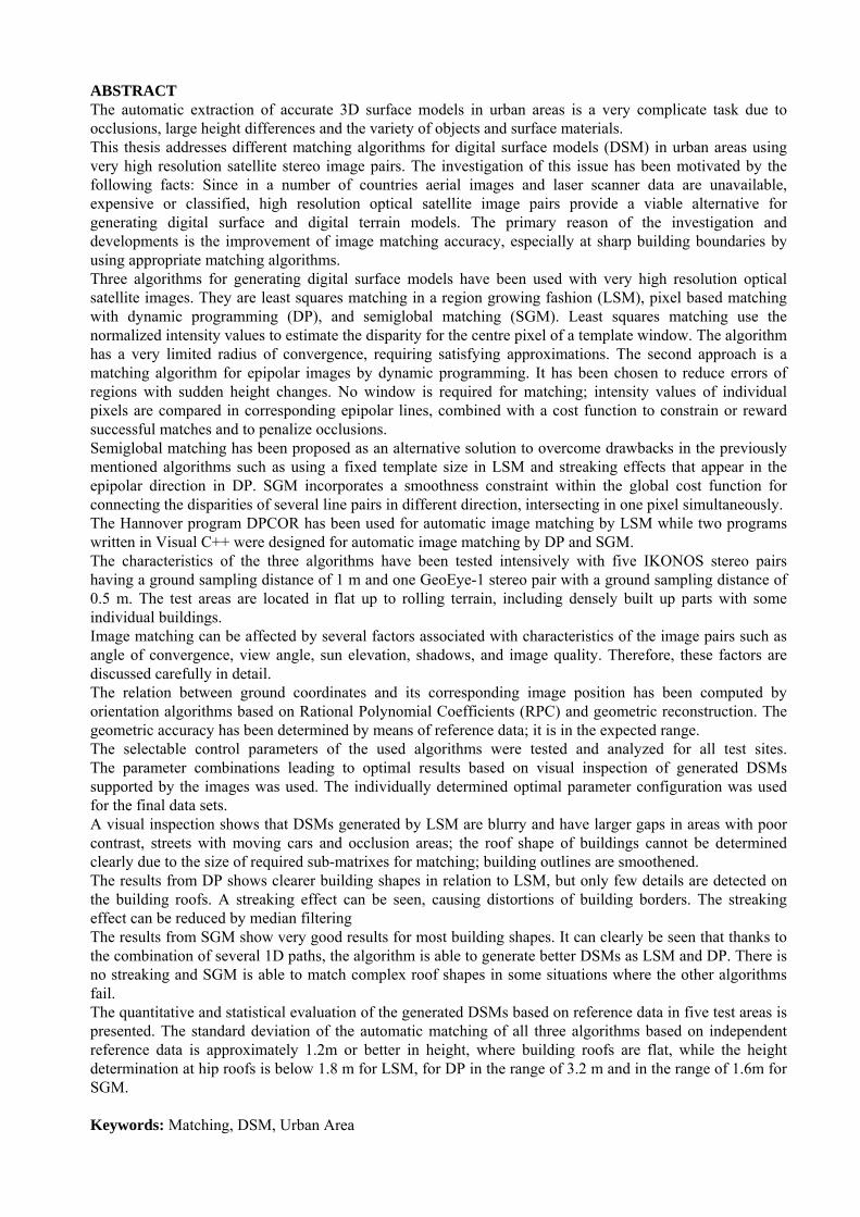
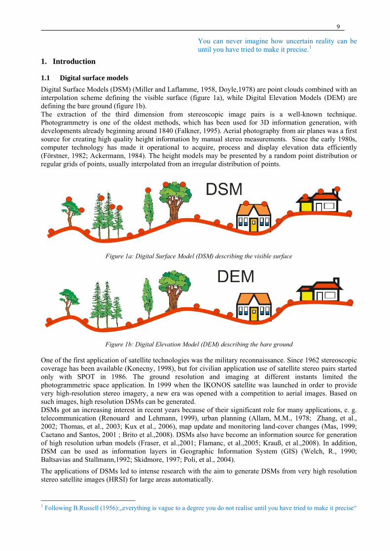
1.1 Digital surface models Digital Surface Models (DSM) (Miller and Laflamme, 1958, Doyle,1978) are point clouds combined with an interpolation scheme defining the visible surface (figure 1a), while Digital Elevation Models (DEM) are defining the bare ground (figure 1b). The extraction of the third dimension from stereoscopic image pairs is a well-known technique. Photogrammetry is one of the oldest methods, which has been used for 3D information generation, with developments already beginning around 1840 (Falkner, 1995). Aerial photography from air planes was a first source for creating high quality height information by manual stereo measurements. Since the early 1980s, computer technology has made it operational to acquire, process and display elevation data efficiently (Förstner, 1982; Ackermann, 1984). The height models may be presented by a random point distribution or regular grids of points, usually interpolated from an irregular distribution of points.

Figure 1a: Digital Surface Model (DSM) describing the visible surface

Figure 1b: Digital Elevation Model (DEM) describing the bare ground

One of the first application of satellite technologies was the military reconnaissance. Since 1962 stereoscopic coverage has been available (Konecny, 1998), but for civilian application use of satellite stereo pairs started only with SPOT in 1986. The ground resolution and imaging at different instants limited the photogrammetric space application. In 1999 when the IKONOS satellite was launched in order to provide very high-resolution stereo imagery, a new era was opened with a competition to aerial images. Based on such images, high resolution DSMs can be generated. DSMs got an increasing interest in recent years because of their significant role for many applications, e. g. telecommunication (Renouard and Lehmann, 1999), urban planning (Allam, M.M., 1978; Zhang, et al., 2002; Thomas, et al., 2003; Kux et al., 2006), map update and monitoring land-cover changes (Mas, 1999; Caetano and Santos, 2001 ; Brito et al.,2008). DSMs also have become an information source for generation of high resolution urban models (Fraser, et al.,2001; Flamanc, et al.,2005; Krauß, et al.,2008). In addition, DSM can be used as information layers in Geographic Information System (GIS) (Welch, R., 1990; Baltsavias and Stallmann,1992; Skidmore, 1997; Poli, et al., 2004). The applications of DSMs led to intense research with the aim to generate DSMs from very high resolution stereo satellite images (HRSI) for large areas automatically.

1 Following B.Russell (1956):„everything is vague to a degree you do not realise until you have tried to make it precise“

10

1.2 Motivation and goal of the research By manual measurements a DEM or a DSM can be generated, but this is extremely time-consuming and not economic, so automation is required. Automatic height determination in built-up areas remains an area of active research in digital photogrammetry. Not all problems of selecting the optimal methods for extracting 3D information with satisfactory accuracy and reliability have been solved. Using HRSI with ground resolution of about one meter or better for DSM generation is still considered a critical task due to limited accuracy and resolution. Occlusions and sun shadows complicate the task. This investigation has been initiated for two primary reasons. The first reason relates to the use of high resolution satellites images for DSM generation instead of other sources such as aerial images or laser scanner data, which in many parts of the world are unavailable, expensive or classified. Stereo pairs from very high resolution satellites such as IKONOS, QuickBird, WorldView1 and GeoEye-1 led the way into a new, not restricted era of generating DSMs. The second reason is a recent revival of image matching (see e.g. (Haala, 2009)), and thus a renewed interest in the capabilities of recently developed algorithms with respect to traditional solutions. An automatic procedure for the generation of DSMs including building shapes based on image matching techniques is highly desirable. Although several matching algorithms have been developed over the last 10 years, none of them solved the correspondence problem completely in complex built-up areas with the limited resolution of space images. The primary aim of the investigation presented here is the generation of urban DSMs based on very high resolution stereoscopic satellite images by three matching algorithms. The main topic is to analyze and compare the proposed matching algorithms. The analysis is based on the comparison of the generated height models in different test areas with reference models. Therefore, this thesis gives an accurate analysis of three used matching algorithms for urban DSM generation from HRSI with their advantages and disadvantages. Based on this investigation, the reader should be able to choose one of them according to his or her application.

1.3 Problem Statement The limitations in generating DSM using very high-resolution stereo satellite images can be summarized as follows:

(1) Photogrammetric orientation: this error component results from sensor models and the accuracy of the image orientation procedure including ground control points.

(2) Image matching accuracy: this result from the selected matching algorithm, used to find conjugate points in stereo pairs and then produce height models based on the locations of corresponding pixels.

(3) Interpolation accuracy: It includes errors resulting from interpolating an elevation at an arbitrary position using directly computed elevation data.

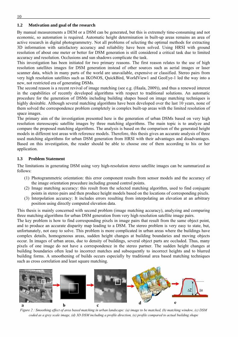
This thesis is mainly concerned with second problem (image matching accuracy), analyzing and comparing three matching algorithms for urban DSM generation from very high resolution satellite image pairs. The key problem is how to find corresponding pixels in image pairs that result from the same object point, and to produce an accurate disparity map leading to a DSM. The stereo problem is very easy to state, but, unfortunately, not easy to solve. This problem is more complicated in urban areas where the buildings have complex details, homogeneous areas, sudden height changes at building boundaries and moving objects occur. In images of urban areas, due to density of buildings, several object parts are occluded. Thus, many pixels of one image do not have a correspondence in the stereo partner. The sudden height changes at building boundaries often lead to incorrect matches and subsequently to incorrect heights and to blurred building forms. A smoothening of builds occurs especially by traditional area based matching techniques such as cross correlation and least square matching.

Figure 2 : Smoothing effect of area based matching in urban landscape: (a) image to be matched, (b) matching window, (c) DSM coded as a grey scale image, (d) 3D DSM including a profile direction, (e) profile compared to actual building shape

11

As shown in figure 2, if a matching window with constant size and shape is used, traditional area based matching algorithms cannot properly determine points at the building outlines. Rather, the resulting DSM is a smoothed version of the actual surface of the urban landscape, because some pixels of the window show parts of the roof while others depict parts of the neighbouring ground.

The problem may become more complex, when high resolution satellite images are used. Today high resolution stereo satellite images achieve a ground sampling distance (GSD) up to 0.50 m (e.g. WorldView1 and GeoEye-1); such a resolution can compete with traditional aerial images so that the space images provide an important source in the absence of more detailed images. However, matching of high resolution satellite scenes in urban areas will be accompanied by some of the challenges which prevent the matching process to be optimal:

• Images of 1m resolution or better possess unique geometric and radiometric characteristics in build up areas due to occlusion (hidden parts), sun shadows, and large differences in height and sudden changes in height.

• Due to geometric difference and occlusion between image pairs, traditional matching algorithms are not appropriate for DSM generation from satellite and aerial imagery (Fraser et al., 2001).

• The use of satellite images not taken at the same day may lead to radiometric differences causing failure of image matching (Jacobsen, 2003).

• Image distortions, which can be related to the platform or sensor noise such as calibration parameters, may lead to incorrect matches if not taken into account.

• The height-to-base ratio and the imaged objects have a significant impact on the DSM quality (Alobeid et al., 2010) where the matching of images with a small angle of convergence shows clearer building outlines than the matching with a large base which may have better height accuracy.

1.4 Thesis structure

This thesis consists of seven chapters as follows: Chapter 1 briefly introduces the definition of Digital Surface Models and some of their applications. The motivations of research and the problem statement are also given. Goals, objectives and scopes of research are stated. Chapter 2 provides a brief overview of the literature on image matching algorithms; an insight into current developments on image matching algorithms is given. This review is restricted to the most relevant algorithms for which results from high resolution satellite images in urban areas have been published.

In chapter 3, matching considerations and general strategies for automated DSM generation from high resolution satellite stereo image pairs are presented.The correspondence problem of matching is formulated, followed by a description of the cost function in each algorithm, and required control parameters.

In chapter 4, the characteristics of the input data, with respect to DSM generation, are firstly described based on building shape and building density. Then, based on this assessment analysis of high resolution satellite images in urban areas and the effect on image matching, several factors associated with image characteristics such as angle of convergence, view angle, sun angle, shadowing, and image quality, are discussed. Also the generation of epipolar images is explained in this chapter. The orientation methods used in this thesis are presented. Finally, the reference data are introduced.

In chapters 5, the algorithms for DSM generation are evaluated with high-resolution satellite imagery, i.e. IKONOS and GeoEye-1. The results obtained by the three matching algorithms in the five test areas are presented. The selectable parameters of the algorithm are tested and analysed for all test sites. The optimal control parameter configuration was used for final tests. The evaluation includes a visual inspection of the generated DSMs.

In chapter 6, the quality of the DSMs generated by the used matching algorithms is compared. The comparison includes a qualitative and a quantitative analysis. In the qualitative analysis, the visual comparison includes three investigations: first a 3D visual analysis of the generated DSMs, secondly, comparison of cross section of the DSMs, and finally, the comparison of sub-areas of gray value coded DSMs in all test areas. The shortcomings and weaknesses of the proposed algorithms are discussed in the summary of qualitative analysis. In the quantitative analysis, the quantitative and statistical evaluation of the DSMs with reference data is presented.

Chapter 7 provides a summary of the research. Directions for further research are suggested; to improve the results and to use the results for building monitoring with differential DSMs for map updating.

12

2. State of the Art

2.1 Overview of Image Matching Algorithms One of the most fundamental problems in photogrammetry is to find pairs of pixels from stereo image pairs that correspond to the same object. The difference of corresponding image positions in epipolar direction is named disparity. If the correspondence problem is solved, the object height can be computed by spatial intersection. Unfortunately, the correspondence problem remains a difficult and complex task. Many algorithms for stereo correspondence have been published, but none of them solves the problem completely. The effort for searching corresponding points in a stereo pair can be reduced by using epipolar images. Epipolar lines are defined by the intersection of the plane including an object point and both projection centers to both image planes. To obtain epipolar images the original images are transformed so that epipolar lines are located in the x-direction with the same y-coordinates for both images. Perspective images not being epipolar can be transformed to epipolar images. This definition is correct for perspective images, but line-scanning images have projection centres different for every scan line so by theory epipolar lines are not possible (Otto and Chau., 1989), hoewever, they can be iteratively approximated. As mentioned, in epipolar images corresponding points have the same y-coordinates, so the corresponding points only have to be searched in the x-direction. In general, matching algorithms are divided into two major classes: Local algorithms (area and feature based) and global algorithms (pixel based with cost function). The most important stereo matching algorithms are explained shortly. The discussion in this part is limited to an overview; therefore, the details of the algorithms are not treated here. There are many general overviews on image matching. Perhaps the best known was published by (Scharstein and Szeliski, 2002) in connection with the Middlebury Stereo Vision Page. In the second part of this chapter, algorithms that have been used to generate urban DSM from high-resolution satellites images are reviewed. In local algorithms (area based), a window is defined around each pixel and the matching is performed based on a comparison of windows including the image neighbourhood of processed pixels. The similarity of both corresponding windows often is defined by the correlation coefficient or the root mean square error of the normalized grey values (Ackermann,1984; Heipke,1996). An example is Least Squares Matching (LSM) In least squares matching corrections of geometric and local radiometric distortions which may be caused by tilted object plane are modelled. Furthermore, LSM can generate matching results with sub-pixel accuracy, which makes it accurate and efficient, as we will see in chapter 3 With a fixed window size it is not possible to detect depth discontinuities with satisfying accuracy. This makes these algorithms fail at rough surfaces and occlusion boundaries. Thus, simple image correlation based on horizontal ground elements (horizontal plane) and least squares matching based on inclined planes cannot solve the special problems in urban areas. Therefore, it is very important to define appropriate windows (in its size or shape) to cope with these problems. Many algorithms of windows adapting their shape have been proposed in the literature (Chan, et al., 2003; Anil, et al., 2007). Kanade and Okutomi (1994) proposed a method where windows adapt their size to avoid the effects of projective distortion and large windows including more intensity variation as required. This algorithm modifies the window size and shape adaptively according to the local intensity and disparity variations. Many algorithms using windows adapting their shape have been proposed in the literature (Otto and Chau,1989; Lane, et al.,1994; Boykov, et al.,1998; Veksler,2003). (Fusiello et al.,1997) presented multiple window methods where the correlation is performed using nine windows having the same size, but different positions in relation to the point of interest (see figure 3).

Figure 3: Nine asymmetric correlation windows. The pixel for which disparity is computed is highlighted

The correlation is done with all nine windows, and the disparity associated with the smallest sum of squared difference (SSD) for each pixel is selected as its final disparity. Unfortunately, this algorithm did not work very well in occluded regions due to not utilizing the uniqueness constraint (Fusiello et al.,1997). Hirschmüller, et al. (2002) have used the same concept of multiple windows, but with some improvements, as reducing the error that occurs when correlation windows overlap at object borders and the author proposed a border correction filter to improve matches at object borders.

13

Despite these amendments, the algorithms have not been able to overcome problems at the edges of objects and in occluded regions. Feature based matching algorithms use two stages. Firstly features (points, edges), together with their attributes are extracted in each image individually. Secondly, corresponding features from stereo images have to be found under certain assumptions regarding the local geometry of the object to be reconstructed (Venkateswar and Chellappa, 1995; Schmid and Zisserman, 1997). Some operators are used in feature based matching to find interest points as: The Moravec operator (Moravec,1977), which is based on the assumption that an interest point has high variances in all directions. The Förstner operator (Förstner, 1982) uses the auto-correlation function to classify the pixels into categories (interest points, edges or region). SIFT (Scale Invariant Feature Transform) operator (David, 2004) which transfors image data into scale-invariant coordinates relative to local features. In general,feature based matching does not lead to object point density required for DSM. Area based matching in general is fast compared with global algorithms (Brown, et al., 2003). Area based matching usually work with small windows (templates). Due to the local nature of mentioned algorithms, they have problems in occlusion areas or in poor or no texture regions. They can produce spurious results if the selection algorithm is not properly formulated. A smoothness constraint is usually not incorporated in these algorithms, nevertheless area based matching incorporates a smoothness of the results caused by the size of the used sub-matrix for matching. Furthermore, due to using windows, problems at object edges and in occluded regions are never totally avoidable; this problem can be suppressed by using some adaptive approaches. Alternatively a pixel based matching is possible. The core of such global matching algorithms lies in a correct definition of the scene model including all the assumptions (smoothness, uniqueness, occlusions, discontinuities). They impose constraints on neighbouring pixels in order to reduce sensitivity in corresponding pixels that fail to match due to occlusion and poor local contrast regions. Therefore, the computation is more complex than that of area based matching (Hirschmüller and Scharstein, 2009). The global algorithms are more time consuming. For this reason, the matching is simplified by using epipolar images, where corresponding image points have the same y`-coordinate. The matching problem is formulated as an energy-minimization problem, where the energy function is defined as:

( , ) ( , ) ( , )data smoothE x y E x y E x y= + (1)

The goal is to find a disparity function d that minimizes this energy, where the data term measures how well the disparity function corresponds to the input stereo images. In other words, the data term computes the cost between a stereo image pair:

( , ) ( , ( , ))data P IE x y M p d x y

∈= ∑ (2a)

where p are pixels of the input image and M (p,d(x,y)) is the matching cost function. While the smoothness term incorporates the smoothness assumptions defined by the scene model, it usually penalizes the differences between neighbouring pixel disparities, which have different disparity values. Once the energy function has been defined, various algorithms can be applied to find its minimum:

( )smooth smoothness assumptionsE d = ∑ (2b)

Some algorithms search for the minimum separately for each epipolar line (e.g. via dynamic programming (DP)), where the algorithms search for the best possible path corresponding to minimum cost. Other algorithms based on epipolar images search for the minimization of a 2D neighbouring nodes, and operate across both vertical and horizontal dimensions, (Cox, et al.,1992 ; Geiger et al.,1995 ;Cox, et al., 1996 ;Bobick and Intille, 1999;Veksler, 2005; Lei, et al., 2006). In Cox’s algorithm (1992), the data term consists of the matching costs evaluated on individual pixels, where the matching costs are derived by a normalized squared error that represents the cost of matching two pixels, while the smoothness term is a fixed penalty for unmatched pixels. The matching problem is solved for each line independently via dynamic programming. In 1996, Cox, et al. modified their algorithms, by not penalizing discontinuities in horizontal and vertical directions, but by enforcing two-dimensional constraints, with the lines below and above a given line beeing used to constrain the minimization. In Geiger et al., (1995), the data term was computed over shifting windows, allowing adaptation to intensity values and location variations. For the smoothness term, they imposed an occlusion constraint where a disparity discontinuity along the epipolar line in one input image always corresponds to an occluded region

14

in the other image (and vice versa). A smearing effect appears when the window size is larger (similar to what was discussed in local matching algorithms). Bobick and Intille,(1999) presented a stereo algorithm that finds occluded regions and matches simultaneously. The data term is computed by comparing mean-normalized windows around each pixel in corresponding lines of stereo images. The absolute grey value differences were used as matching costs. By using windows, some problems can occur especially at sudden changes in height, leading to matching errors. The authors try to overcome this problem by using adaptive windows (Fusiello et al., 1997, discussed above).The best path which corresponds to minimum cost through the disparity space image is computed. Veksler, (2005) used the concept of a 2D optimization in horizontal and vertical direction provided by DP, with optimization on a tree to avoid optimization on a graph with loops. The data term consists of the matching costs evaluated on individual pixels, where matching costs were derived by the absolute difference of gray value. A streaking effect that usually appears in epipolar direction due to missing interconnection of neighboured epipolar lines can be avoided, where the estimated disparity at each pixel depends on the estimated disparity for all other pixels that are connected to this pixel in the tree, while in the case of 1D optimization, the estimated disparity depends only on pixels located in corresponding epipolar lines. Hence, the optimization on trees is more efficient than that on a one dimensional array. Lei, et al.,(2006) combined a region-based stereo method and dynamic programming on a tree. Their algorithm consist of two steps. In the first step, a region tree is built on an over-segmented image based on the mean shift method (Christoudias, et al., 2002). Each region in the image is a homogeneous region which is assumed to have the same disparity. In the second step, the optimization on trees (Veksler, 2005) is used, but instead of formulating an image as a pixel tree (Veksler, 2005),the authors propsed a region tree structure, where nodes of trees are the segmented regions. However, this algorithm assumed that pixels within each region have the same disparity, leading to less satisfying results. The minimization of 2D functions to produce a disparity map can be done also graph-based algorithm, minimizing directly 2D functions to produce a disparity surface (Pollard, et al.,1985; Ishikawa and Geiger,1998 ; Boykov et al., 1999). Due to the enormous computational costs for minimizing the 2D function, these algorithms are very slow and and far from real time. In general one of the advantages of global matching is that it provides global support for lacking regions as occlusion and poor local contrast regions. By enforcing some constraints in horizontal and vertical direction, dynamic programming can find the global minimum. 1D dynamic programming suffers from a streaking effect that appears in epipolar direction, causing distortions of object borders when there is no interconnection of neighboured epipolar lines, when the minimization depends only on pixels located in one epipolar line. On the other hand, a smearing effect appears when dynamic programming uses a window.

2.2 Application of satellite images in urban areas

A number of investigations have been done for generating DSM in urban areas by automatic image matching of satellite images. Despite the advances in state of art matching algorithms, the use of high-resolution satellites images, to generate urban DSMs is still difficult. It is not guaranteed that all these algorithms work well with satellite images, which frequently have larger incidence angles and occlusions and are influenced by sun shadows. Only a limited number of publications which deals with systematic comparisons of existing algorithms are available (Krauß et al., 2007, Heipke et al., 2007). In the following recent developments to generate urban DSMs from high-resolution satellites images are reviewed. This review is restricted to the most relevant methods for which results from high resolution satellite images in urban areas were published. The discussion of algorithms applied to urban DSM generation is categorized into: local matching (area based) algorithms and global matching algorithms.

2.2.1 Local matching algorithms

Area based matchers are still the main tool for stereo DSM generation in photogrammetric applications. Area matching usually employs a correlation which includes normalization of radiometry. One popular algorithm to address such issues is a technique to minimise the squared sum of the normed gray value differnces between two image patches as well as to generate appropriate distortion parameters (Grün,1985) – the already mentioned least squares matching. Otto and Chau (1989) proposed an algorithm where the approximations for LSM are determined by region growing. The approach requires seed points (start points for matching), which were provided by manual measurement in both images. The basic idea behind this algorithm is to select the best of the nearest matched points and then matches the four neighbouring points at a pre-defined interval, subsequently continuing at the point with highest correlation coefficient. The algorithm, also employed by (Heipke et al.,1996) for

15

MEOSS data, works quite well when the terrain does not include sudden height changes and the matched points are close together. A similar algorithm can also be found in (Trinder et al., 1994). The knowledge of several surrounding matched points is spread to the expected points by using a simple transformation function. This algorithm avoids the problem of relying on the knowledge of only one matched point ,but still it may not work well in case of very steep terrain or low density of matched points, which makes it difficult for use in urban area where sudden height changes at building boundaries often lead to incorrect matches or voids.

(Li and Grün, 2004) suggested multi-image matching for DSM generation from IKONOS imagery. As preparation the local contrast was improved by Wallis filtering. The approximation problem is solved by image pyramids and feature based matching of points, grids and free form lines. Suitably well-defined feature points are extracted using the Förstener interest operator (Förstener and Gülch, 1987) and by using geometric constrained cross-correlation (Grün, 1985). Edge extraction is based on the Canny operator (Canny, 1986) and independently linked into free-form edges. Then a triangular irregular network (TIN) is created by combining all matched edges and feature points. The final shape of matching is a grid point matching able to fill gaps in regions with poor texture. A refinement by least squares matching is carried out to achieve more precise object points. The authors add only local smoothness constraints so the problems at building boundaries have not been solved, leading to ambiguities at building boundaries. (Poon et al., 2005) , (Zhang and Grün , 2006) and (Zhang and Fraser, 2008) use this algorithm to generate DSMs from high resolution satellite imagery. As reference a Lidar DSM is used. Their investigations did not focus on the shape of buildings. Furthermore, the algorithm doesn’t suggest solutions for problems that occur at buildings boundaries. Rau and Chen (2005) generated a DSM from IKONOS imagery based on the hierarchical matching window strategy (Chen, et al.,1994). In order to reduce the effect of a fixed size of matching window, they propose adaptive windows, where the algorithm modifies the window size and shape adaptively according to the local intensity and disparity variations. LSM has been adopted to solve the correspondence problem. Unfortunately, the accuracy of the generated DSM is not analyzed, and the smearing effect of area based matching remained due to using windows.

Jacobsen (2006) and (Büyüksalih and Jacobsen, 2007) used least squares matching in a region growing fashion, their work has mainly focused on the impact of matching parameters and the influence of IKONOS stereo image properties on the DSM accuracy. They did not suggest solutions for problems that occur at buildings boundaries. Krauß, et al., (2007) used area based matching to generate a DSM from IKONOS imagery. The approximation problem is solved by image pyramids and feature based matching, while the matching is area based with fixed window size. Due to the use of a window of constant shape, the algorithm leads to incorrect matches at shape edges and subsequently to incorrect height models as well as to blurred building forms. (Rozycki and Wolniewicz , 2009) compared four commercial software packages that can generate DSM from IKONOS imagery. The following programs were used in their investigation: PCI Geomatica 10, ERDAS Imagine 8.7, Leica Photogrammetry Suite 9 and Photomod 4.1. Their investigation has mainly focused on comparison of general height over large areas (300km2) by using also Ground Control Points (GCP) as reference. Their comparison did not include any comparison of building shapes.

2.2.2 Global matching algorithms

A number of investigations have been done concerning the comparison of matching algorithms to generate a DSM in urban areas. Before very high resolution satellite images were available, for example (Benard, et al., 1986) compared the performances of dynamic programming (using the Viterbi algorithm; Forney, 1973) and the vertical line locus (Wullschleger, 1986).

Baillard and Dissard (2000) proposed a method where the basic idea was to combine edge and area based matching, and to take occlusions into account along epipolar lines using dynamic programming. At first, they matched edge pairs using a cost function and applied area based matching between the matched edge points. This area-based matching stage works in two consecutive steps, one is radiometrically constrained in order to produce only reliable pairs and the other is geometrically constrained in order to complete the matching on unmatched areas. The edge matching detects height discontinuity and tries to preserve the building outline. Area based matching is used to produce a dense elevation model which is used to verify the edge based matching result. The final geometrically constrained matching reduces the gaps in homogenous areas. By using scanned aerial photos with a ground sampling distance of 40 cm, which is close to the ground distance of satellite images such as GeoEye-1 or WorldView1, the authors show very

16

encouraging DSM results. But it is not clear if this algorithm works well with high-resolution satellite stereo images, which frequently have larger incidence angles and occlusions. Kim et al. (2002) generated urban DSM from IKONOS images by using a graph-cut algorithm in 3D voxel space based on a global energy minimization scheme. Instead of defining 3D energy spaces they used the direction of disparity and 2D image space to estimate an optimal disparity as the minimum cut of the maximum flow within the energy space (as is the general case in graph cut). They supposed two adjacent voxels, where the voxel centers have been projected to the left and right images for obtaining the projected pixels. This idea helps to overcome problems caused by a very large baseline between the satellite images. In this algorithm, heights in shadow areas were not estimated by graph cut but are interpolated as average heights from the surroundings. The advantage of this algorithm is the possibility to recover building heights better than area based matching, but disadvantages are: (1) Graph-cut produces some blunders in areas containing homogeneous patterns. (2) Graph cut is mathematically complex and far from real time. (3) Graph cut can not work on the full IKONOS stereo image size due to limited memory, hence the image need to be split into small windows.

Krauß et al., (2005; 2008) proposed an algorithm for DSMs generation from IKONOS images. The authors adapted the idea of dynamic line warping from an older work in the field of speech recognition, called dynamic time warping (Sakoe and Chiba, 1978). They compared intensities of corresponding epipolar line pairs instead of recorded speech sequences and calculated a matching cost by taking the absolute difference of intensities. Then, the optimal path with minimal cost was determined using dynamic programming. The advantage of this algorithm is the possibility to use windows around every line position which can give better results than taking individual lines only, but disadvantages are: (1) a streaking effect, known from dynamic programming, appears in the epipolar direction, causing distortion of building borders, (2) a smearing effect appears when the window size is larger, (3) no smoothness constraints have been included, leading to ambiguities at building boundaries where the height changes suddenly. This method requires epipolar images.

Chehata et al. (2005; 2009) proposed an algorithm that can generate DSMs from high resolution satellite images which have submeter resolution (45-70 cm) and a simulated height to base(h/b) ratio (5-20). The algorithm focuses on how to find building roofs, as well as the ground surface without handling the facade extraction of buildings, which are too complex in satellite images. The global optimization by graph cut is usually done on pixel information in 2D images, but this algorithm uses the combination of 3D features (3D segments, planar facets) and 2D images, where 3D features are used as constraints to guide the optimization process in a 3D graph. The 3D segments are extracted from images by an algorithm described in (Chehata et al., 2002). The 3D segments correspond to building borders. The extraction of the features is reliable but not necessarily dense. The estimated height by 3D segments is not robust with a small angle of convergence (Chehata et al., 2002), for this reason, only planimetric coordinates of segments are used. In fact, the algorithm is designed for aerial images, where details on building roofs appear clearly. The authors applied the algorithm to aerial images, simulating satellite images with 50 cm resolution. However, it is not clear if this algorithm works well with satellite images, which frequently have larger incidence angles. In addition, they did not suggest any solution to overcome the problems resulted due to a very large baseline in satellite images.

17

2.3 Discussion Although several matching algorithms have been developed over last 20 years, none of them solves the problem in complex built-up areas with limited ground resolution completely. Most existing area based algorithms, working with a fixed window size, adaptive or multiple windows show poor reliability at building boundaries, because they assume that the object heights for all pixels in the correlation window is in a horizontal or tilted plane, leading to distortions at building edges. In dense urban areas, many buildings are very complex to be modelled. Additional constraints should be added to support spatial smoothness. Global matching algorithms have been employed to avoid problems related to area based matching by matching individual pixels. However, it is anticipated that some of those algorithms comparing intensities of corresponding epipolar line pairs individually, commonly suffer from a streaking effect in epipolar direction, causing distortions of building borders because of missing interconnection of neighbored epipolar lines, while other algorithms try to avoid problems related to area based matching by minimizing an energy function imposing constraints on neighbouring pixels in order to reduce pixels that fail to match due to occlusion or missing texture in 2D. Therefore, the computation will be more complex than area based matching. Most mentioned algorithms are based on the absolute differences or squared differences of grey values to measure correspondence costs. Such cost functions are very sensitive to radiometric differences caused by illumination and reflection which is frequent in satellite images in urban area. Therefore, to reduce the influence of radiometric differences, an alternative matching scheme should be used such as Mutual Information (MI) that measures correspondence without assuming that conjugate points to have the same intensity values (Viola and Wells, 1997; Kim et al., 2003). Semiglobal matching (SGM) is a new image matching algorithm, which originated from the computer vision community. It has been developed by Hirschmüller (2006, 2008). SGM computes conjugate points along multiple conjugate lines hierarchically by using mutual information instead of intensity value differences as dissimilarity measure. SGM has been proposed as an alternative solution to overcome the drawbacks at building outlines. SGM reduces the well-known streaking effects, which occurs in DP.

18

3. Description of Matching Algorithms and General Strategy for Matching

Matching considerations and a general strategy for automated DSM generation from high resolution satellite stereo images will be presented in this chapter.

Stereo matching for generating a DSM of dense urban areas from high resolution satellite stereo images led to the selection of three algorithms for the analysis: a traditional one, a well known global solution, and a recently published promising approach:

• Least squares matching (LSM; Förstner, 1982) in a region growing fashion (Otto and Chau, 1989; Heipke et al., 1996), an area based algorithm which compares the normalized intensity values within a template to those in a search window. LSM is reported to be accurate and efficient as it can generate matching results with sub-pixel accuracy relatively fast. Moreover, a linear radiometric correction and linear geometric distortion between stereo images is considered in this algorithm.

• Dynamic programming (DP) according to (Birchfield and Tomasi, 1999), a global algorithm which determines pixel disparities in epipolar lines by searching for best paths through the related cost matrix based on individual pixel intensity values as input for a dissimilarity measure. It has been chosen to reduce errors at regions of sudden height changes where LSM is known to perform poorly. In this way the number and the effect of errors in the vicinity of sudden height changes should be limited because of additional support in these regions;

• Semiglobal matching (SGM), (Hirschmüller, 2006; 2008), which computes conjugate points along multiple conjugate lines hierarchically by using mutual information instead of intensity value differences as dissimilarity measure. SGM reduces the well-known streaking effects of DP.

These algorithms were selected based on their general characteristics and popularity rather than for their suitability for the given task alone. The known main problems of LSM (blurred height discontinuities) and DP (streaking) are investigated for their application to high resolution satellite images such as IKONOS.

3.1 Least squares matching with region growing (LSM)

3.1.1 Matching strategy

This area based algorithm (Förstner, 1982) uses the normalized intensity values to estimate the disparity for the centre pixel of a template window. The algorithm has a very limited radius of convergence, requiring relatively accurate initial values.

Matching using LSM with region growing requires at least one seed point (start point for matching). Seed points are points of interest, improved by least squares matching. LSM transforms the template window of one image to the other by affine transformation. In addition, the constant and linear intensity value differences between both template windows are determined, allowing a computation of the correlation coefficient of the best fit of both template windows.

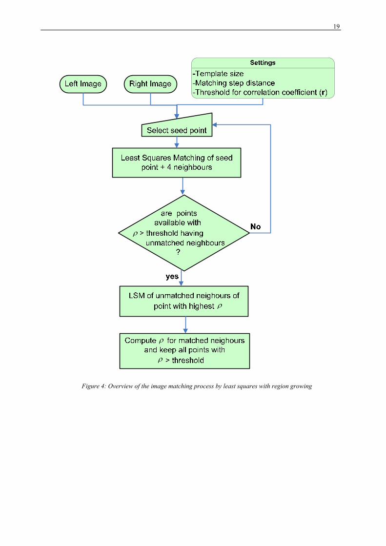
From the seed point, four neighbouring points at a pre-defined interval are matched, and subsequently from the point with the highest correlation coefficient of all neighbours, ideally continued up to a complete coverage of the stereo model. Matching is only continued with points having a correlation coefficient exceeding a specified threshold, to avoid a matching of areas without sufficient contrast or without sufficient similarity. An overview of the matching process by LSM with region growing is shown in figure 4. Least square matching is used for determining homologous points between the template and the matching window by minimizing the normalized intensity values value differences.

Besides the seed point, the window size, the matching step distance, and the threshold for the correlation coefficient were an important parameters for the success of this algorithm (see 3.1.4). Therefore good values of these parameters have to be found.

19

ρ

ρ

ρ

ρ

Figure 4: Overview of the image matching process by least squares with region growing

20

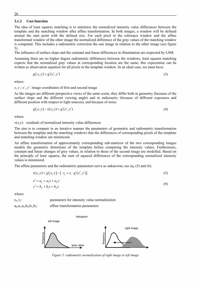
3.1.2 Cost function The idea of least squares matching is to minimize the normalized intensity value differences between the template and the matching window after affine transformation. In both images, a window will be defined around the start point with the defined size. For each pixel in the reference window and the affine transformed window of the other image the normalized difference of the gray values of the matching window is computed. This includes a radiometric correction the one image in relation to the other image (see figure 5). The influence of surface slope and the constant and linear differences in illumination are respected by LSM. Assuming there are no higher degree radiometric differences between the windows, least squares matching expects that the normalized gray values at corresponding location are the same; this expectation can be written as observation equation for all pixels in the template window. In an ideal case, we must have:

( ), (́ ,́ )́g x y g x y= (3)

where: x, y ; x´, y´: image coordinates of first and second image As the images are different perspective views of the same scene, they differ both in geometry (because of the surface slope and the different viewing angle) and in radiometry (because of different exposures and different position with respect to light sources), and because of noise.

( ), ( , ) (́ ,́ )́g x y v x y g x y− = (4)

where: v(x,y): residuals of normalized intensity value differences The aim is to compute in an iterative manner the parameters of geometric and radiometric transformation between the template and the matching windows that the differences of corresponding pixels of the template and matching window are minimized. An affine transformation of approximately corresponding sub-matrices of the two corresponding images models the geometric distortions of the template before comparing the intensity values. Furthermore, constant and linear changes of grey values, in relation to those of the second image are modelled. Based on the principle of least squares, the sum of squared differences of the corresponding normalized intensity values is minimized. The affine parameters and the radiometric parameters serve as unknowns; see eq. (5) and (6).

( ) 1( , ) , [ (́ ,́ )́]ov x y g x y r r g x y= − + ⋅ (5)

1 2

1 2

''

o

o

x a a x a yy b b x b y

= + +

= + + (6)

where: r0, r1: parameters for intensity value normalization a0,a1,a2,b0,b1,b2: affine transformation parameters

freq u

ency

f requ

ency

gray value

left image

right image

histogram

Figure 5: radiometric normalization of right image to left image

21

The histogram of gray values of the actual window in the right image will be transformed together with the geometric relation to the left image by the function: ( ) 1, [ (́ ,́ )́]og x y r r g x y= + ⋅ . The position and the shape of the template are changed until the normalized gray level differences reach a minimum. The centre positions of both actual windows are used as corresponding image points.

3.1.3 Acceptance criteria for the similarity The threshold for the correlation coefficient between the first and the resampled second window serves as criteria for accepting the optimization. In LSM the threshold for the correlation coefficient depends upon the similarity of the images, which may be poor if there is a larger time interval of the imaging instant. The normalized cross-correlation coefficient ρ is calculated by the formula:

( )( )( )

1 1

2 2 1/ 21 1 1 1

( , ( , ))( (́ ,́ )́ ( ,́ )́)

( , ( , )) . ( (́ ,́ )́ ( ,́ )́) ][r c

i jr c r c

i J i J

g x y g x y g x y g x y

g x y g x y g x y g x yρ = =

= = = =

− −=

− −

∑ ∑∑ ∑ ∑ ∑

(7)

where:

ρ : normalized cross-correlation coefficient (values: -1 ≤ ρ ≤ 1)

( , ), ( ,́ ´)g x y g x y : mean intensity values of the first and second image.

c, r: number of rows and columns of template.

A correlation coefficient of the corresponding sub-matrixes of +1 indicates a perfect match, while -1 indicates an inverse correlation. A correlation coefficient value near zero indicates a non-match. When the matching process is performed, a matching success rate can be calculated by:

100%. accepted

overlap

Matching success NN

= × (8)

where: Naccepted :Number of pixels with correlation coefficient exceeding the specified correlation threshold Noverlap: number of possible points in the overlapping region of both images (same spacing as Naccepted) The matching success gives the percentage of pixels that have correlation coefficient exceeding the specified correlation coefficient threshold within the overlapping area. A good choice of threshold value and window size will increase the matching success rate. If the ratio is low, the selected parameters must be amended within the allowed limits.

3.1.4 Control parameters A good choice of the matching window size and threshold for correlation coefficient is essential for the success of the algorithm. Seed points: in theory the region growing strategy requires only one pair of homologous points as start values. However, more pairs are required in reality, because the region growing may stop in areas with large height differences or with low contrast. The number of required seed points depends on image similarity and decreases with a larger height-to-base (h/b) ratio corresponding to a smaller angle of convergence. Window size: As the matching cost depends on the properties of the matching window, therefore, the size of the matching window is important. Due to the use of a template with constant size (corresponding to a tilted plane in 3D space), the algorithm is not able to match points of building outlines (showing height discontinuities), leading to smoothed building shapes. In particular for larger window sizes, adjacent buildings may be merged and appear as a common blob. A smaller template may circumvent this problem to a certain extent and thus yield more correct results near height discontinuities, but generally leads to a lower accuracy because of the reduced redundancy of the adjustment.

22

Matching step distance: The row-step and column-step (integer pixel) are used for region growing. In relation to the seed point or the point which just has been handled, the algorithm will go in up to 4 directions to neighboured positions with a distance in the image identical to row-step and column-step. The step width should depend upon the roughness of the terrain.

In images of urban areas, due to the density of buildings and sudden height changes at building boundaries, the matching step distance of one pixel leads to more reliable results, although the processing time will increase and neighboured points are strongly correlated because of overlapping windows. Threshold for correlation coefficient: The threshold for the correlation coefficient plays an important role for the success of this algorithm. It can easily be determined empirically based on frequency distribution of correlation coefficients (Jacobsen, 2006). If it is too high, the success rate will be low, if is too low, the number of blunders will increase. The frequency distribution of the correlation coefficients usually indicates very well the required limit. The control parameters of LSM with region growing are summarized in the table 1.

Parameter

Description Range

Seed points start points for matching

• depends on image similarity • number decreases with a larger

(h/b) ratio • number increases with large

height differences

Window size Part of image which will be compared with other image

5×5 pixel2- 20×20 pixel2

Matching step width Used value for region growing

1×1 pixel- 3×3 pixel

Threshold for correlation coefficient

criterion for accepting the results of LSM

0.60 - 0.90

Table 1: User-defined parameters for least squares matching with region growing, description and reasonable range

23

3.2 Dynamic Programming (DP)

3.2.1 Matching strategy

The second investigated approach is a matching algorithm for epipolar images by dynamic programming (Birchfield and Tomasi, 1999). It has been chosen to reduce errors at regions of sudden height changes, e.g. at building outlines where LSM is known to perform poorly. No windows are required for matching; intensity values of individual pixels are compared in corresponding epipolar lines, combined with constraints to reward successful matches and to penalize occlusions. The algorithm focuses especially on generating correct results at height discontinuities, sacrificing some accuracy in smooth areas.

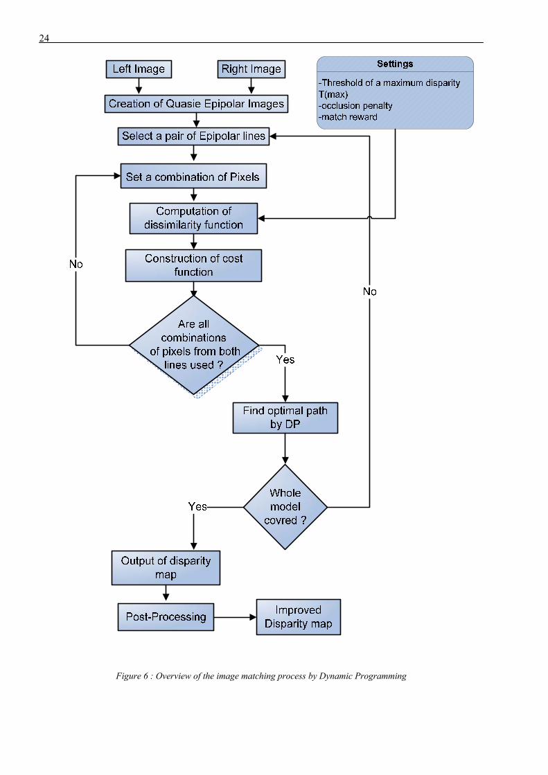
In order to obtain the desired disparity map from high resolution satellite imagery, the matching strategy goes as follows (see figure 6):

• Creation of epipolar images in order to benefit from the advantage of epipolar images where the matching pixels between the images appear along a common x axis and the possibility of incorrect matches can be reduced. Moreover the speed of the matching process also will increase. Quasi-epipolar images from satellite images projected to a plane with constant height have been generated by rotating the stereo images to the base direction of the scene centre lines as will be described in section (4.3).

• Threshold for the minimum and maximum disparity are required; the latter value should exceed the

maximum disparity in the scene depending upon building and terrain heights and h/b ratio. This means that the algorithm will not look for pixels that are shifted more than this threshold. Therefore if the distance between left and right pixels is larger than a threshold for the maximum disparity, the algorithm will be limited to the threshold for the maximum disparity.

• The algorithm matches epipolar lines independently. Each epipolar line of an image is represented as a

profile of gray values, and then each pixel in the left epipolar line is compared to some pixels of the conjugate epipolar line where the distance between them does not exceed the threshold for the maximum disparity. The dissimilarity between the pixels is computed according to eq. (12),and then a 2D array of costs is constructed according to eq. (9)

• A path of minimum cost through the 2D array is determined using dynamic programming to find the

proper correspondence. The path detection is conducted from the left side to the right side of the 2D array of costs and the optimum path is searched within a neighbourhood corresponding to the maximum allowed absolute disparity.

• The correspondence is encoded in a sequence of models, where each match is an ordered pair (X,Y) of pixels indicating that the intensities in left and right epipolar lines are images of the same scene point. Then the disparity map can be computed.

• The previous steps will be repeated for each corresponding epipolar line, until the whole model covered.

• In order to remove a streaking effect in epipolar direction, which causes distortions of building borders because there is no interconnection of the epipolar lines, the results are post-processed by using a median filtering perpendicular to the epipolar line direction (vertical median filter).

24

Figure 6 : Overview of the image matching process by Dynamic Programming

25

3.2.2 Cost function calculation

Matching is formulated as an optimization problem for each corresponding epipolar line pair independently based on a pre-defined cost function to be minimized. Each pixel in the left epipolar line is compared to some pixels of the conjugate epipolar line, and a 2D array of costs is constructed. The matching cost measures how unlikely it is that the pixels in the left epipolar lines and pixels in the right epipolar lines are an image of the same object point. The used cost function (X,Y)λ has three components, see eq. (9):

m 1

-X Y = ( , ) ( , ) m

i i r occocc

N

iN Nd X Y K Kλ × ×

=+∑ (9)

X, Y are the image coordinates of the epipolar image The first component is the sum of the dissimilarities ( , )i id X Y between the matched pixels, it should

dominate the cost function. The second component ( m rN K× ) is a reward for correct matching, where Nm is the number of matched

pixels and Kr is the match reward per pixel. The third component ( occoccN K× ) is a penalty for occlusions, where Nocc is the number of occlusions (not

the number of occluded pixels) and Kocc is the occlusion penalty. The parameters of the algorithms do not have an explicit physical meaning, thus an empirical determination is necessary. Kr is the maximum amount of pixel dissimilarity expected between two correctly matched pixels, while Kocc is the evidence to declare an occlusion and thus a change in disparity. The two parameters (Kocc, Kr) have an important role in calculating the matching costs which in turn specifies the disparity; these values are sensitive to intensity values of corresponding pixels.

3.2.2.1 Pixel dissimilarity

The easiest dissimilarity function is the absolute value of difference in intensities. Instead, the dissimilarities by using linearly interpolated intensities halfway between the pixels in each corresponding epipolar line and its neighbors, is computed according to (Birchfield and Tomasi, 1998) to overcome sampling effects (see figure 7).

Figure 7 : computation of pixel dissimilarity

In this discussion, Xi with intensity IL and Yi with intensity IR are chosen as the pixels whose dissimilarity is to be measured.

First, the term { }( ) ( 1)21

R R RI Yi I YiI−

= + − is computed which represents linearly interpolated intensity

halfway between the pixel Yi and its neighbors to left in right epipolar line.

The analogous term { }( ) ( 1)21

R R RI Yi I YiI+

= + + is computed between the pixel Yi and its neighbors to the

right in right epipolar line. Then two terms can be computed from the pervious terms:

min max( ) ( ), , .. . ,. ,min maxR R R Yi R R R YiandI I I I I II I− + − +⎧ ⎫ ⎧ ⎫= =⎨ ⎬ ⎨ ⎬

⎩ ⎭ ⎩ ⎭ , with these terms defined:

26

{ }) m( , , , max 0 ( ) I I ( ), ,L R L max in LXi Yi Id I I Xi I Xi−

= − − (10)

In the same manner, all the terms ( , , II ,L L min maxI I− +

) of the left epipolar line are calculated. With these terms

on the left epipolar line, the dissimilarity is calculated:

{ }) m( , , , max 0 ( ) I I ( ), ,R L R max in RYi Xi Id I I Yi I Yi−

= − − (11)

Finally, the minimum of equations (10, 11) can be calculated:

) )( , ) ( , , ( , ,min{ , , , }L R R Ld Xi Yi Xi Yi I Yi Xi Id I d I− −

= (12)

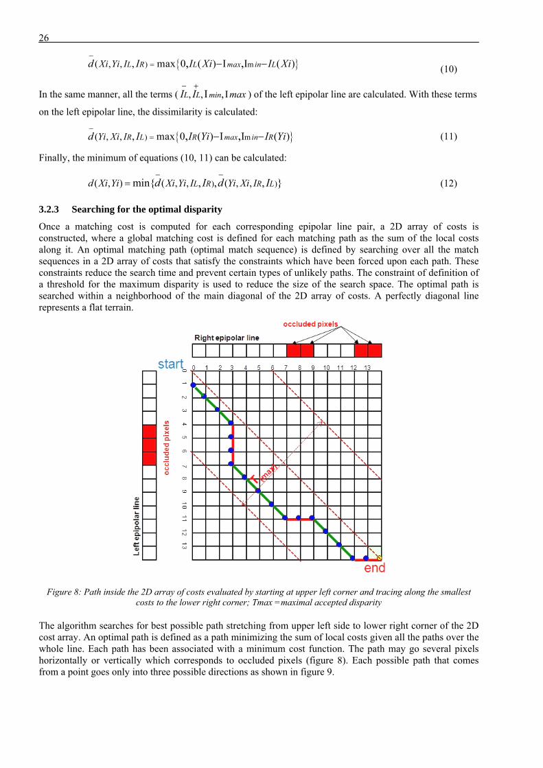
3.2.3 Searching for the optimal disparity

Once a matching cost is computed for each corresponding epipolar line pair, a 2D array of costs is constructed, where a global matching cost is defined for each matching path as the sum of the local costs along it. An optimal matching path (optimal match sequence) is defined by searching over all the match sequences in a 2D array of costs that satisfy the constraints which have been forced upon each path. These constraints reduce the search time and prevent certain types of unlikely paths. The constraint of definition of a threshold for the maximum disparity is used to reduce the size of the search space. The optimal path is searched within a neighborhood of the main diagonal of the 2D array of costs. A perfectly diagonal line represents a flat terrain.

Figure 8: Path inside the 2D array of costs evaluated by starting at upper left corner and tracing along the smallest costs to the lower right corner; Tmax =maximal accepted disparity

The algorithm searches for best possible path stretching from upper left side to lower right corner of the 2D cost array. An optimal path is defined as a path minimizing the sum of local costs given all the paths over the whole line. Each path has been associated with a minimum cost function. The path may go several pixels horizontally or vertically which corresponds to occluded pixels (figure 8). Each possible path that comes from a point goes only into three possible directions as shown in figure 9.

27

Figure 9 : Three possible paths through a 2D array of costs, the horizontal axis corresponds to the right epipolar line and the vertical axis corresponds to the right epipolar line

where: Path 1: means that the disparity of the pixel x1 in the position (n, m) is the same as the disparity of the pixel x2 in the position (n-1,m-1); they are on a horizontal 3D surface. Path 2: means that the path moved one pixel forward on left image, keeping the same position on the right one, this means that a part of the left image does not appear on the right one. Path3: is the opposite of path 2, regarding left line and right line. Once these matches are found a disparity map can be computed that shows how far each pixel in the left epipolar line is moved when matched to its corresponding pixel in the right epipolar line.

3.2.4 Postprocessing the disparity map: 1D dynamic programming handles epipolar line pairs independently, so a streaking effect appears in epipolar line direction, causing distortions of building borders. The results can been post-processed by using a median filtering with a width of one pixel in the epipolar line direction and a specified number of pixels across the epipolar line direction (vertical median filter) to reduce this streaking effect.

3.2.5 Control parameters The parameters of the algorithms have been selected according to the characteristics of each stereo pair, an empirical determination has been used. Threshold for the maximum disparity: This value should exceed the maximum disparity in the scene depending upon terrain plus building height and h/b ratio. A good choice of a threshold for the maximum disparity value has an important role in determining the quality of the output disparity map and also influences the computation time. The two parameters occ ( , )rK K have an important role in calculating the matching costs which in turn specifies the disparity. These values are sensitive to intensity values of corresponding pixels. In general, changes in height and occlusions in urban areas are visible as intensity changes, for this reason payment of a penalty occK preserves height changes and corresponding occlusions: Each change in height incurs an occlusion penalty and since the algorithm imposes a penalty on each occlusion rather than for each occluded pixel, the approach sacrifices height changes in homogeneous regions.The parameters used for DP are summarized in the table 2.

Parameter Description Range

Threshold for the maximal disparity[T(max)]

maximum expected disparity value to recovered height of an stereo image

• depends on building and terrain height and h/b ratio

• increases with height building

Match reward [ ]rK The maximum amount of pixel dissimilarity expected between two correctly matched pixels

[2 - 14] pixels

Penalty for occlusions [ ]occK The evidence to declare an occlusion and thus a change in disparity

[4 - 21] pixels

Table 2 : User-defined parameters for Dynamic Programming, description and reasonable range

28

3.3 Semiglobal Matching (SGM)

3.3.1 Matching Strategy It is known that both described algorithms (LSM and DP) have principal difficulties in providing high quality DSMs as discussed above: for LSM the main problem is the template, for DP streaking effects appear in the epipolar direction. Semiglobal matching (SGM; Hirschmüller, 2006; 2008) has been proposed as an alternative solution to overcome these drawbacks. SGM requires epipolar geometry; it incorporates a smoothness constraint within the global cost function for connecting the disparities of several line pairs of different direction, intersecting in one pixel simultaneously. In order to obtain the desired disparity map from high resolution satellite imagery, the matching strategy is divided for the following stages (see figure 10):

• Generation of epipolar images, to benefit from the advantage of epipolar images where the matching pixels between the images appear along a common x axis and the possibility of incorrect matches can be reduced. Moreover, the speed of the matching process also increases. Quasi epipolar images have been generated by rotating the stereo images to the base direction of the scene centre lines, as will be described in section 4.3.

• An initial disparity image that is required for warping one of the stereo images is computed hierarchically (details are following in 3.3.2). Downscaling by factor 24 =16 is done by averaging over 16x16 Pixel. The computed disparity image is upscaled by factor 2 and used as initial disparity image for matching image at scale 23.The process is repeated until the full resolution has been reached where the scale is 20 = 1.

• The matching costs are computed based on Mutual Information (MI). MI depends upon the entropy and joint entropy of the pixels in a stereo pair (details are following in 3.3.2).

• The aggregation matching costs are computed, where the aggregated (smoothed) cost for each pixel is computed by summing the costs of all minimum cost of all intersecting lines at the pixel. Global 2D smoothness constraints were added to support the smoothness by penalizing changes of neighbouring disparities between neighboring pixels. The number of accumulated paths should be at least 8 or 16 for providing a good coverage of the 2D image. Each path starts at each border pixel of the image and is traversed in the chosen direction. All accumulated paths are calculated sequentially to provide a good coverage of the 2D image. The minimization is realized by aggregating of pathwise costs into a cost cube.

• The disparity image that corresponds to the base image (left image in the flow chart that is shown in figure 10) is constructed by selecting for each pixel the disparity that corresponds to the minimum cost from the cost cube. Optional the warping can be made in addition also with reverse image.

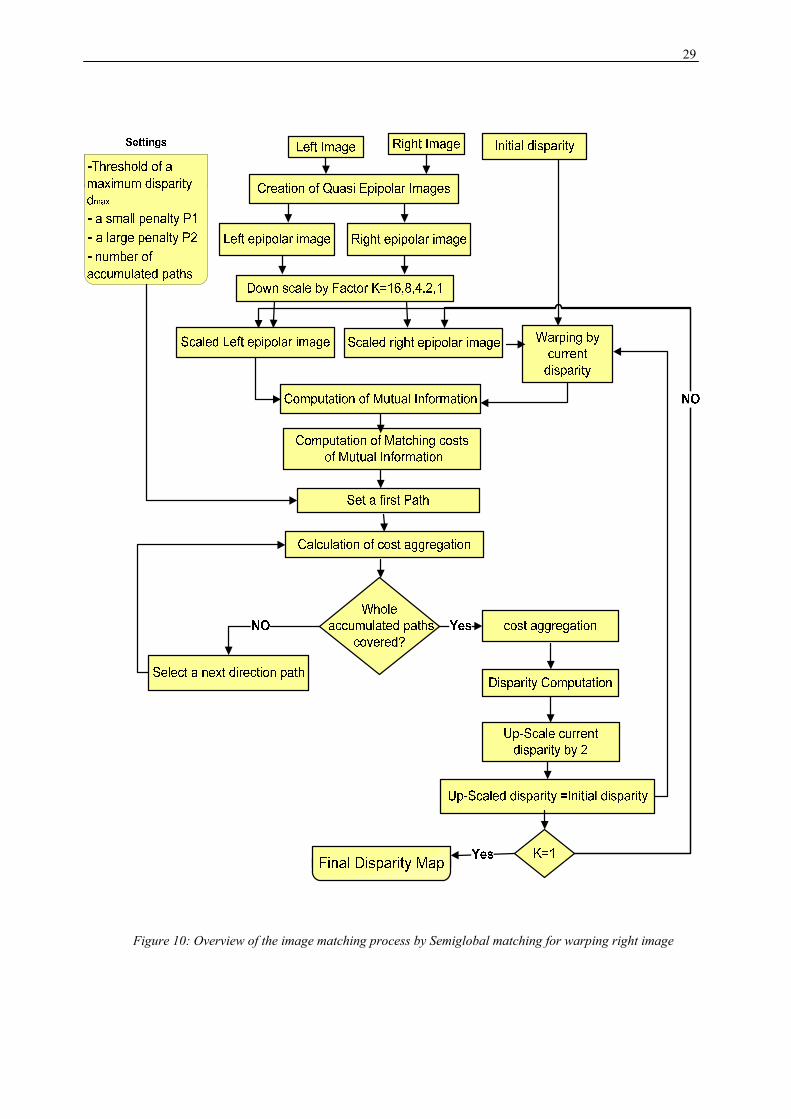
29

Figure 10: Overview of the image matching process by Semiglobal matching for warping right image

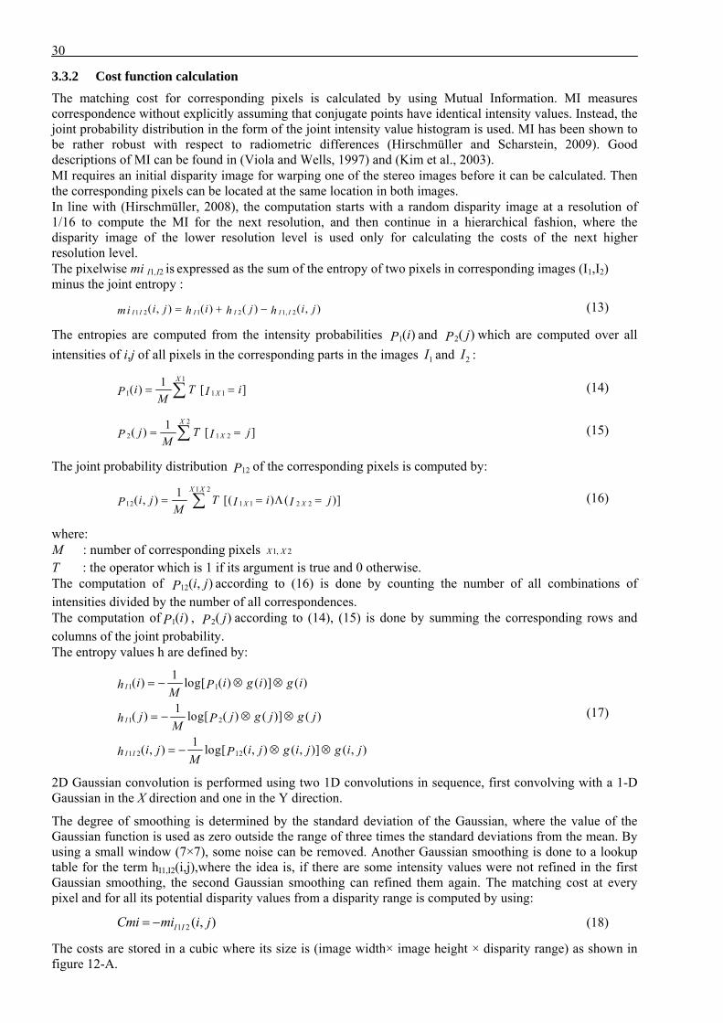
30

3.3.2 Cost function calculation The matching cost for corresponding pixels is calculated by using Mutual Information. MI measures correspondence without explicitly assuming that conjugate points have identical intensity values. Instead, the joint probability distribution in the form of the joint intensity value histogram is used. MI has been shown to be rather robust with respect to radiometric differences (Hirschmüller and Scharstein, 2009). Good descriptions of MI can be found in (Viola and Wells, 1997) and (Kim et al., 2003). MI requires an initial disparity image for warping one of the stereo images before it can be calculated. Then the corresponding pixels can be located at the same location in both images. In line with (Hirschmüller, 2008), the computation starts with a random disparity image at a resolution of 1/16 to compute the MI for the next resolution, and then continue in a hierarchical fashion, where the disparity image of the lower resolution level is used only for calculating the costs of the next higher resolution level. The pixelwise mi I1,I2 is expressed as the sum of the entropy of two pixels in corresponding images (I1,I2) minus the joint entropy :

1 2 1 2 1, 2( , ) ( ) ( ) ( , )I I I I I Ii j i j i jmi h h h= + − (13)

The entropies are computed from the intensity probabilities 1( )iP and 2( )jP which are computed over all intensities of i,j of all pixels in the corresponding parts in the images 1I and 2I :

1

1 1 11( ) [ ].

X

Xi T iP IM= =∑ (14)

2

2 1 21( ) [ ].

X

Xj T jP IM= =∑ (15)

The joint probability distribution 12P of the corresponding pixels is computed by: 1 2

12 1 1 2 21( , ) [( ) ( )].

X X

X Xi j T i jP I IM= = Λ =∑ (16)

where: M : number of corresponding pixels 1, 2X X T : the operator which is 1 if its argument is true and 0 otherwise. The computation of 12( , )i jP according to (16) is done by counting the number of all combinations of intensities divided by the number of all correspondences. The computation of 1( )iP , 2( )jP according to (14), (15) is done by summing the corresponding rows and columns of the joint probability. The entropy values h are defined by:

11

21

121 2

1( ) log[ ( ) ( )] ( )

1( ) log[ ( ) ( )] ( )

1( , ) log[ ( , ) ( , )] ( , )

I

I

I I

i i g i g ih PM

j j g j g jh PM

i j i j g i j g i jh PM

= − ⊗ ⊗

= − ⊗ ⊗

= − ⊗ ⊗

(17)

2D Gaussian convolution is performed using two 1D convolutions in sequence, first convolving with a 1-D Gaussian in the X direction and one in the Y direction.

The degree of smoothing is determined by the standard deviation of the Gaussian, where the value of the Gaussian function is used as zero outside the range of three times the standard deviations from the mean. By using a small window (7×7), some noise can be removed. Another Gaussian smoothing is done to a lookup table for the term hI1,I2(i,j),where the idea is, if there are some intensity values were not refined in the first Gaussian smoothing, the second Gaussian smoothing can refined them again. The matching cost at every pixel and for all its potential disparity values from a disparity range is computed by using:

1 2 ( , )I ICmi mi i j= − (18)

The costs are stored in a cubic where its size is (image width× image height × disparity range) as shown in figure 12-A.

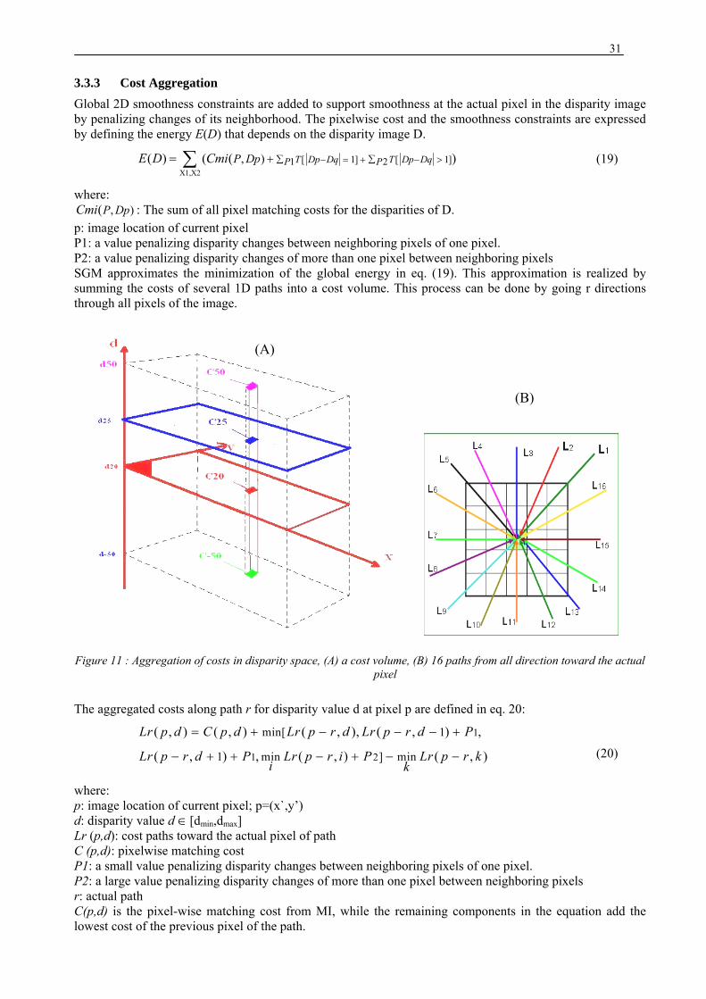
31

3.3.3 Cost Aggregation Global 2D smoothness constraints are added to support smoothness at the actual pixel in the disparity image by penalizing changes of its neighborhood. The pixelwise cost and the smoothness constraints are expressed by defining the energy E(D) that depends on the disparity image D.

X1,X2[ 1] [ 1]1 2, )( ) ( ( )T Dp Dq T Dp DqP PP DpE D Cmi ∑ ∑− = + − >+= ∑ (19)

where: , )(P DpCmi : The sum of all pixel matching costs for the disparities of D.

p: image location of current pixel P1: a value penalizing disparity changes between neighboring pixels of one pixel. P2: a value penalizing disparity changes of more than one pixel between neighboring pixels SGM approximates the minimization of the global energy in eq. (19). This approximation is realized by summing the costs of several 1D paths into a cost volume. This process can be done by going r directions through all pixels of the image. The aggregated costs along path r for disparity value d at pixel p are defined in eq. 20:

1

1 2

min[ 1

1 min ] min

( , ) ( , ) ( , ), ( , ) ,

( , ) , ( , ) ( , )

Lr p d C p d Lr p r d Lr p r d P

Lr p r d P Lr p r i P Lr p r ki k

= + − − − +

− + + − + − − (20)

where: p: image location of current pixel; p=(x`,y’) d: disparity value d ∈[dmin,dmax] Lr (p,d): cost paths toward the actual pixel of path C (p,d): pixelwise matching cost P1: a small value penalizing disparity changes between neighboring pixels of one pixel. P2: a large value penalizing disparity changes of more than one pixel between neighboring pixels r: actual path C(p,d) is the pixel-wise matching cost from MI, while the remaining components in the equation add the lowest cost of the previous pixel of the path.

(A)

(B)

Figure 11 : Aggregation of costs in disparity space, (A) a cost volume, (B) 16 paths from all direction toward the actual pixel

32

The aggregation costs from all direction over all paths are computed: '

1( , ) ( , )

r

ri

S p d p dL=

= ∑ (21)

r`: number of paths The number of accumulated paths must be at least 8 or 16 for providing a good coverage of the 2D image (Hirschmüller, 2006). Each path starts at each border pixel of the image, and the image is traversed in the chosen direction. All accumulated paths are calculated sequentially to provide a good coverage of the 2D image (see figure 11-B). The minimization is realized by aggregating of pathwise costs in the cost volume (see figure 11-B). The important aspects of SGM are: • No windows are required, since for matching individual pixels in corresponding epipolar lines are used. • The optimization is carried out for several line intersecting in one pixel simultaneously to reduce

streaking effects. • Additional constraints are added to support building shapes: a small additional cost P1 is added if the

disparity changes only by one pixel with respect to the neighborhood, whereas a larger cost P2 is added when the disparity changes by more than one pixel.

• The penalty P2 does not depend on the actual disparity. In this way larger height discontinuities, which often occur at building boundaries, are allowed.

• Matching costs can be computed via MI or anther cost function such as the squared or absolute intensity differences.

3.3.4 Optimal disparity The final disparity image is then selected as index of the minimum cost from the cost volume according to eq. (22):

{ }( , ) ( , )mind

D x y S p d= (22)

This disparity image corresponds to the left image, if the left image is considered as base image and a right image has been warped. However, in the case of warping the left image, the right image will be considered as a base image; the disparity image should be calculated from scratch, where the matching cost and aggregation matching costs are calculated again. This step permits the possibility to determine occlusions and false matches. To remove remaining outliers that can be included in a disparity image, finally a 3×3 median filter is used.

3.3.5 Control parameters Satisfying control parameter values are required for good performance of the algorithm. Traditionally the optimal parameters are determined by tried and error. Visual inspection of the initial disparity with original image provides an impression about quality of selected parameter values. The used ranges of parameters for SGM are summarized in table 3 Parameter Description Range

Threshold for maximal disparity[d(max)]

maximal expected disparity value in the stereo model

• depends on building and terrain height and h/b ratio

• increases with height variation

Number of accumulated path [r]

number of accumulated paths that provide a good coverage of the 2D image

[8 or 16]

P1 penalty for changes in disparity of one pixel [3 - 11]

P2 penalty for changes in disparity of more than one pixel [3 - 13]

Table 3 : User-defined parameters for SGM, description and reasonable range

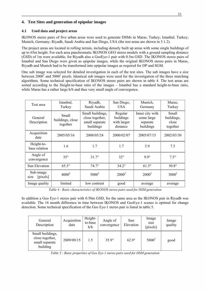
33

4. Test Sites and generation of epipolar images

4.1 Used data and project areas

IKONOS stereo pairs of five urban areas were used to generate DSMs in Maras, Turkey; Istanbul, Turkey; Munich, Germany; Riyadh, Saudi Arabia and San Diego, USA (the test areas are shown in 5.1.2).

The project areas are located in rolling terrain, including densely built up areas with some single buildings of up to 65m height. For each area panchromatic IKONOS GEO stereo models with a ground sampling distance (GSD) of 1m were available, for Riyadh also a GeoEye-1 pair with 0.5m GSD. The IKONOS stereo pairs of Istanbul and San Diego were given as epipolar images, while the original IKONOS stereo pairs in Maras, Riyadh and Munich had to be transformed into epipolar images as required for DP and SGM.

One sub image was selected for detailed investigation in each of the test sites. The sub images have a size between 20002 and 50002 pixels. Identical sub images were used for the investigation of the three matching algorithms. Some technical specification of IKONOS stereo pairs are shown in table 4. The test areas are sorted according to the Height-to-base ratio of the images – Istanbul has a standard height-to-base ratio, while Maras has a rather large h/b and thus very small angle of convergence.

Test area Istanbul, Turkey

Riyadh, Saudi Arabia

San Diego, USA

Munich, Germany

Maras, Turkey

General Description

Small buildings, close

together

Small buildings, close together, small separate

buildings

Regular buildings

with larger distance

Inner city with some large

separate buildings

Small buildings,

close together

Acquisition date 2005/05/16 2008/05/24 2000/02/07 2005/07/15 2002/03/30

Height-to-base relation 1.6 1.7 1.7 5.9 7.5

Angle of convergence 35° 31.7° 32° 9.9° 7.5°

Sun Elevation 65.5° 74.7° 34.2° 61.5° 50.8°

Sub-image size [pixels] 40002 50002 20002 20002 30002

Image quality limited low contrast good average average Table 4 : Basic characteristics of IKONOS stereo pairs used for DSM generation

In addition a Geo Eye-1 stereo pair with 0.50m GSD, for the same area as the IKONOS pair in Riyadh was available. The 16 month difference in time between IKONOS and GeoEye-1 scenes is optimal for change detection. Some technical specification of the Geo Eye-1 stereo pair is listed in table 5.

General Description

Acquisition date

Height-to-base

h/b

Angle of convergence

Sun Elevation

Image size

[pixels]

Image quality

Small buildings, close together, small separate

building

2009/09/15 1.5 35.9° 62.9° 50002 good

Table 5 : Basic properties of Geo Eye-1 stereo pairs used for DSM generation

34

4.2 Parameters influencing image matching

Image matching is affected by several factors associated with characteristics of the images such as angle of convergence, view angle, sun angle, shadowing, and image quality. These factors play a crucial role for the generation of digital surface models from very high resolution satellites images.

4.2.1 Angle of convergence

The angle of convergence is formed by the intersection of two image rays that intersect at a ground target point.

Figure 12 : Relation between convergence angle (α) and h/b

where: a = angle of convergence and ß=horizontal angle In the case of a smaller angle of convergence, the images of a stereo scene are more similar, improving the matching results. On the other hand a larger angle of convergence by geometrically improves the height accuracy, but it enlarges the disparity, causing some matching problems (Jacobsen, 2003).

4.2.2 View angle

The pixel size of satellite image depends upon the nadir angle, for satellite images more precisely on the elevation or incidence angle. With the original object pixel size for nadir view of 0.81m for IKONOS, the object pixel size reaches 1m in view direction for an elevation angle δ of 64.2° (formula in figure 13). In orbit direction the object pixel size depends upon the sampling rate which may lead to an oversampling.

A larger nadir angle generates larger occlusions - some facades may be visible in one image, but not in the other. This leads to some image pixel having no conjugate pixel in the other image. Occlusion is a main source of mismatches independent upon matching methods.

ν = nadir angle δ = elevation angle incidence angle = 90° - δ PN = object pixel size for view to nadir PV = object pixel size in view direction PA = object pixel size across view direction PV = PN / sin² δ PA = PN / sin δ Component of projected pixel size across base direction = PV×sinß + PA×cos ß

Figure 13 : geometric condition nadir and elevation angle

4.2.3 Image quality Image quality refers to the possibility to identify objects in the images, where the variation of the pixel grey values influences the image matching. The signal variation in shadows depends upon the situation of the atmosphere, where very clear atmosphere leads to dark shadows with poor information. The contrast of the IKONOS images in the Riyadh test area is limited; nevertheless the image quality is satisfying for all test areas. The matching has been done without pre-processing of the images in all test sites.

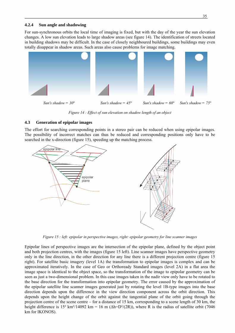
35

4.2.4 Sun angle and shadowing

For sun-synchronous orbits the local time of imaging is fixed, but with the day of the year the sun elevation changes. A low sun elevation leads to large shadow areas (see figure 14). The identification of streets located in building shadows may be difficult. In the case of closely neighboured buildings, some buildings may even totally disappear in shadow areas. Such areas also cause problems for image matching.

Sun's shadow = 30° Sun's shadow = 45° Sun's shadow = 60° Sun's shadow = 75°

Figure 14 : Effect of sun elevation on shadow length of an object

4.3 Generation of epipolar images

The effort for searching corresponding points in a stereo pair can be reduced when using epipolar images. The possibility of incorrect matches can thus be reduced and corresponding positions only have to be searched in the x-direction (figure 15), speeding up the matching process.

Figure 15 : left: epipolar in perspective images, right: epipolar geometry for line scanner images

Epipolar lines of perspective images are the intersection of the epipolar plane, defined by the object point and both projection centres, with the images (figure 15 left). Line scanner images have perspective geometry only in the line direction, in the other direction for any line there is a different projection centre (figure 15 right). For satellite basic imagery (level 1A) the transformation to epipolar images is complex and can be approximated iteratively. In the case of Geo or Orthoready Standard images (level 2A) in a flat area the image space is identical to the object space, so the transformation of the image to epipolar geometry can be seen as just a two-dimensional problem. In this case images taken in the nadir view only have to be rotated to the base direction for the transformation into epipolar geometry. The error caused by the approximation of the epipolar satellite line scanner images generated just by rotating the level 1B-type images into the base direction depends upon the difference in the view direction component across the orbit direction. This depends upon the height change of the orbit against the tangential plane of the orbit going through the projection centre of the scene centre – for a distance of 15 km, corresponding to a scene length of 30 km, the height difference is 15² km²/14092 km = 16 m (Δh=D²/(2R)), where R is the radius of satellite orbit (7046 km for IKONOS).

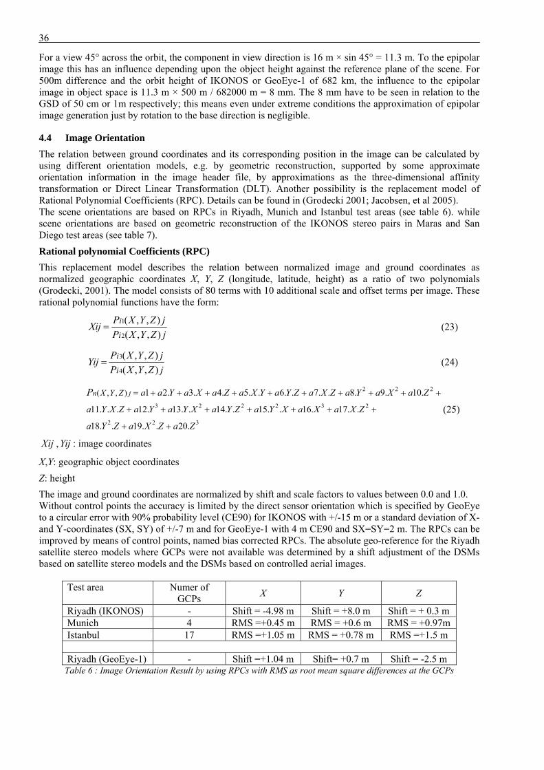
36

For a view 45° across the orbit, the component in view direction is 16 m × sin 45° = 11.3 m. To the epipolar image this has an influence depending upon the object height against the reference plane of the scene. For 500m difference and the orbit height of IKONOS or GeoEye-1 of 682 km, the influence to the epipolar image in object space is 11.3 m × 500 m / 682000 m = 8 mm. The 8 mm have to be seen in relation to the GSD of 50 cm or 1m respectively; this means even under extreme conditions the approximation of epipolar image generation just by rotation to the base direction is negligible.

4.4 Image Orientation The relation between ground coordinates and its corresponding position in the image can be calculated by using different orientation models, e.g. by geometric reconstruction, supported by some approximate orientation information in the image header file, by approximations as the three-dimensional affinity transformation or Direct Linear Transformation (DLT). Another possibility is the replacement model of Rational Polynomial Coefficients (RPC). Details can be found in (Grodecki 2001; Jacobsen, et al 2005). The scene orientations are based on RPCs in Riyadh, Munich and Istanbul test areas (see table 6). while scene orientations are based on geometric reconstruction of the IKONOS stereo pairs in Maras and San Diego test areas (see table 7). Rational polynomial Coefficients (RPC) This replacement model describes the relation between normalized image and ground coordinates as normalized geographic coordinates X, Y, Z (longitude, latitude, height) as a ratio of two polynomials (Grodecki, 2001). The model consists of 80 terms with 10 additional scale and offset terms per image. These rational polynomial functions have the form:

1

2

( , , )( , , )

i

i

P X Y Z jXijP X Y Z j

= (23)

3

4

( , , )( , , )

i

i

P X Y Z jYijP X Y Z j

= (24)

2 2 2

3 2 2 2 3 2

2 2 3

( , , ) 1 2. 3. 4. 5. . 6. . 7. . 8. 9. 10.

11. . . 12. 13. . 14. . 15. . 16. 17. .

18. . 19. . 20.

n jX Y Z a a Y a X a Z a X Y a Y Z a X Z a Y a X a Z

a Y X Z a Y a Y X a Y Z a Y X a X a X Z

a Y Z a X Z a Z

P = + + + + + + + + + +

+ + + + + + +

+ +

(25)

Xij ,Yij : image coordinates

X,Y: geographic object coordinates Z: height The image and ground coordinates are normalized by shift and scale factors to values between 0.0 and 1.0. Without control points the accuracy is limited by the direct sensor orientation which is specified by GeoEye to a circular error with 90% probability level (CE90) for IKONOS with +/-15 m or a standard deviation of X- and Y-coordinates (SX, SY) of +/-7 m and for GeoEye-1 with 4 m CE90 and SX=SY=2 m. The RPCs can be improved by means of control points, named bias corrected RPCs. The absolute geo-reference for the Riyadh satellite stereo models where GCPs were not available was determined by a shift adjustment of the DSMs based on satellite stereo models and the DSMs based on controlled aerial images.

Test area Numer of GCPs X Y Z

Riyadh (IKONOS) - Shift = -4.98 m Shift = +8.0 m Shift = + 0.3 m Munich 4 RMS =+0.45 m RMS = +0.6 m RMS = +0.97m Istanbul 17 RMS =+1.05 m RMS = +0.78 m RMS =+1.5 m Riyadh (GeoEye-1) - Shift =+1.04 m Shift= +0.7 m Shift = -2.5 m

Table 6 : Image Orientation Result by using RPCs with RMS as root mean square differences at the GCPs

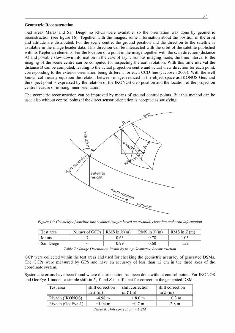
37

Geometric Reconstruction

Test areas Maras and San Diego no RPCs were available, so the orientation was done by geometric reconstruction (see figure 16). Together with the images, some information about the position in the orbit and attitude are distributed. For the scene centre, the ground position and the direction to the satellite is available in the image header data. This direction can be intersected with the orbit of the satellite published with its Keplerian elements. For the location of a point in the image together with the scan direction (distance A) and possible slow down information in the case of asynchronous imaging mode, the time interval to the imaging of the scene centre can be computed for respecting the earth rotation. With this time interval the distance B can be computed, leading to the actual projection centre and actual view direction for each point, corresponding to the exterior orientation being different for each CCD-line (Jacobsen 2003). With the well known collinearity equation the relation between image, realized in the object space as IKONOS Geo, and the object point is expressed by the relation of the IKONOS Geo position and the location of the projection centre because of missing inner orientation.

The geometric reconstruction can be improved by means of ground control points. But this method can be used also without control points if the direct sensor orientation is accepted as satisfying.

Figure 16: Geometry of satellite line scanner images based on azimuth, elevation and orbit information

Test area Numer of GCPs RMS in X (m) RMS in Y (m) RMS in Z (m) Maras 7 0.63 0.78 1.05 San Diego 6 0.99 0.60 1.52

Table 7 : Image Orientation Result by using Geometric Reconstruction

GCP were collected within the test areas and used for checking the geometric accuracy of generated DSMs. The GCPs were measured by GPS and have an accuracy of less than 12 cm in the three axes of the coordinate system.

Systematic errors have been found where the orientation has been done without control points. For IKONOS and GeoEye-1 models a simple shift in X, Y and Z is sufficient for correction the generated DSMs.

Test area shift correction in X (m)

shift correction in Y (m)

shift correction in Z (m)

Riyadh (IKONOS) -4.98 m + 8.0 m + 0.3 m Riyadh (GeoEye-1) +1.04 m +0.7 m -2.8 m

Table 8: shift correction in DSM

38

4.5 Reference Data In order to carry out a qualitative and statistical analysis of DSMs generated by the three matching algorithms described in chapter 3, accurate reference data have to be available. Different reference data were used in this investigation.

4.5.1 Building database Reference data for Istanbul were obtained from a building database with one height per building (see figure 17), generated by manual photogrammetric measurements from UltraCamD images acquired in 2006. The planimetric standard deviation of the building outline coordinates is 0.6 GSD, determined at independent check points (Dursun et al., 2008), which corresponds to 18 cm in object space, while the vertical accuracy is about of 30 cm.

Figure 17 : Building Database in Istanbul test area

It should be noted that the standard deviation of the building heights is somewhat larger due to the influence of the roof landscape.

4.5.2 Creation of reference DSMs based on aerial images For the Riyadh test area, a DSM was generated by using aerial photos taken in May 2007 by an analogue aerial camera RC30. The aerial images were available at a scale 1/5500 (focal length =303.2 mm), scanned at 14 μm corresponding to a ground sampling distance (GSD) of 7 cm. The stereo pairs have of 60% forward overlap and 20% side lap .The image quality of the scanned grainy analogue aerial images was improved by an average Filter (4×4 filter window), reducing the image noise. The DSMs are generated by LSM with image orientation given from a bundle block adjustment. LSM was used because of processing time and the very high resolution of 7 cm. The bundle block adjustment is with 2.7 µm σ0and means square discrepancies at GCPs of 1.0 cm for X, 1.1 cm for Y and 4.4 cm in Z. The DSM has been used as a reference to compare the geometric accuracy of DSMs generated by the three matching algorithms from IKONOS and GeoEye-1 images in the Riyadh test area.

4.5.3 The manually measured stereo model For San Diego test area, IKONOS stereo pairs were imported into the Leica Photogrammetry Suite (LPS). Using RPCs provided by the vendor and information included in the metadata files; both the interior and exterior orientation parameters are automatically computed for use in the aerial triangulation. Building heights were measured manually in the IKONOS stereo model based on the parallax between the two points. The achieved vector data include the height difference between the point on the roof and corresponding ground point. The accuracy of these reference measurements is estimated to be approximately 0.6 m, as determined from repeated measurements.

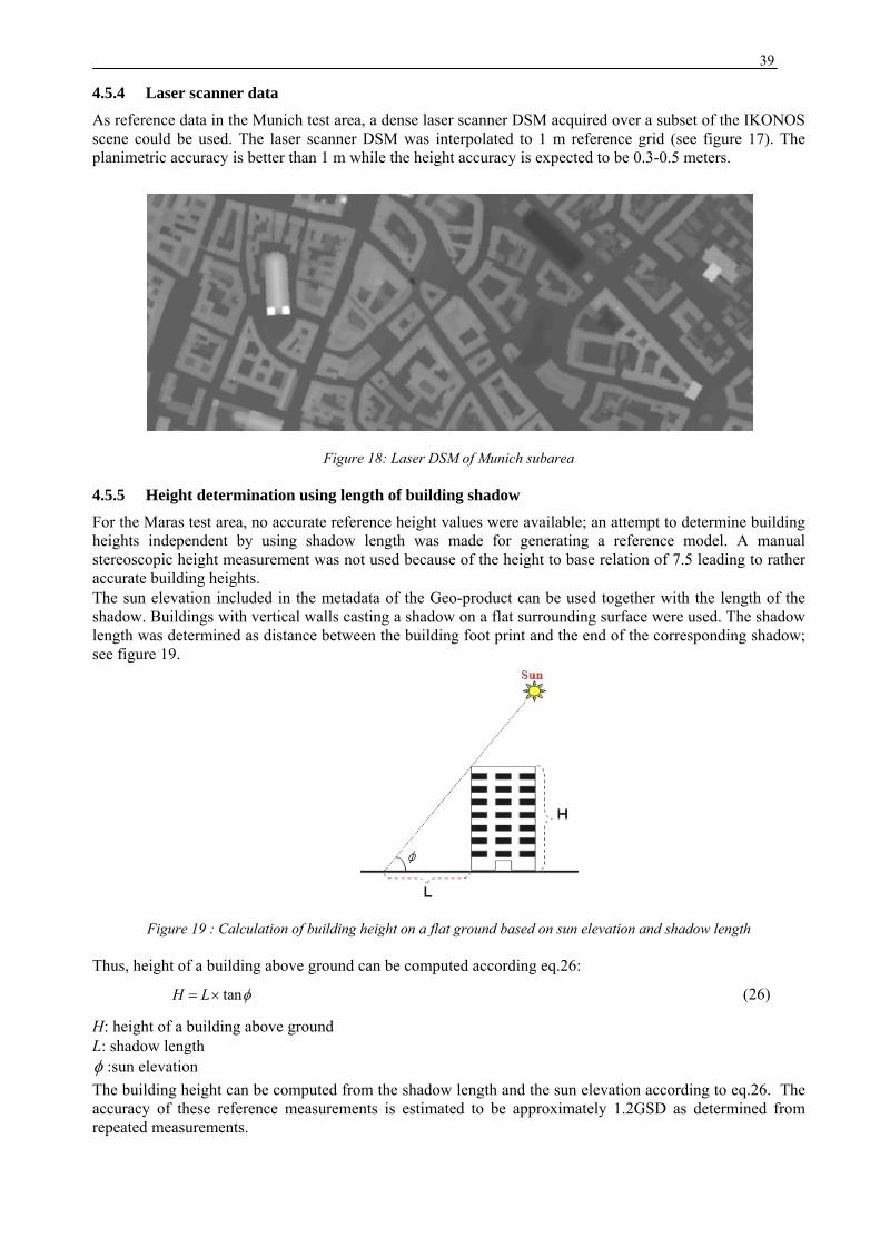
39

4.5.4 Laser scanner data

As reference data in the Munich test area, a dense laser scanner DSM acquired over a subset of the IKONOS scene could be used. The laser scanner DSM was interpolated to 1 m reference grid (see figure 17). The planimetric accuracy is better than 1 m while the height accuracy is expected to be 0.3-0.5 meters.

Figure 18: Laser DSM of Munich subarea

4.5.5 Height determination using length of building shadow

For the Maras test area, no accurate reference height values were available; an attempt to determine building heights independent by using shadow length was made for generating a reference model. A manual stereoscopic height measurement was not used because of the height to base relation of 7.5 leading to rather accurate building heights. The sun elevation included in the metadata of the Geo-product can be used together with the length of the shadow. Buildings with vertical walls casting a shadow on a flat surrounding surface were used. The shadow length was determined as distance between the building foot print and the end of the corresponding shadow; see figure 19.

Figure 19 : Calculation of building height on a flat ground based on sun elevation and shadow length

Thus, height of a building above ground can be computed according eq.26:

tanH L φ= × (26)

H: height of a building above ground L: shadow length φ :sun elevation The building height can be computed from the shadow length and the sun elevation according to eq.26. The accuracy of these reference measurements is estimated to be approximately 1.2GSD as determined from repeated measurements.

40

4.5.6 Discussion Here the comparison of the vertical accuracy of the generated DSMs is discussed, while the planimetric influence of scene orientation accuracy is not taken into account here. The vertical accuracy of the reference data should be considered in the DSM analysis if it is not well below that of the investigated DSM. By using the formula for error propagation the influence on the DSM accuracy can be estimated:

2 2 2DSM DSM ref refσ σ σ−= − (27)

The vertical accuracy of the reference data are summarized in Table 9

Reference data in test area

Reference data accuracy

Building database, Istanbul

0.30 m

DSMs based on aerial images, Riyadh

0.20 m

Laser scanner DSM, Munich

0.30 m

Manual measured of stereo model, San Diego

0.60 m

Height of buildings determined by using shadow length, Maras

1.20 m

Table 9: vertical accuracy of the reference data

According to the author’s experience the accuracy of manually DSM generated from IKONOS images can be estimated for areas with satisfying contrast with:

( ) 0.5DEM zhGSDb

σ = × × (28)

If the influence of the reference data shall not exceed 5% of the accuracy of the investigated heights, according to formula 27 the reference data must have an accuracy not exceeding 1/3 of the accuracy of the investigated heights. Table 9 shows that the vertical accuracy of all reference data is below this acceptable value for each reference except for height of buildings determined by using shadow length and the manually measured stereo model. In absence of better alternatives, these reference data have still been used.

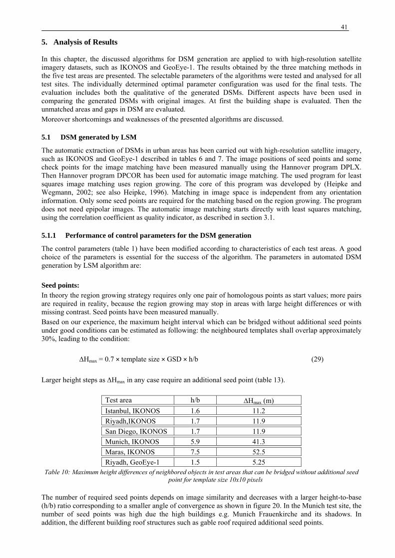
41

5. Analysis of Results

In this chapter, the discussed algorithms for DSM generation are applied to with high-resolution satellite imagery datasets, such as IKONOS and GeoEye-1. The results obtained by the three matching methods in the five test areas are presented. The selectable parameters of the algorithms were tested and analysed for all test sites. The individually determined optimal parameter configuration was used for the final tests. The evaluation includes both the qualitative of the generated DSMs. Different aspects have been used in comparing the generated DSMs with original images. At first the building shape is evaluated. Then the unmatched areas and gaps in DSM are evaluated. Moreover shortcomings and weaknesses of the presented algorithms are discussed.

5.1 DSM generated by LSM

The automatic extraction of DSMs in urban areas has been carried out with high-resolution satellite imagery, such as IKONOS and GeoEye-1 described in tables 6 and 7. The image positions of seed points and some check points for the image matching have been measured manually using the Hannover program DPLX. Then Hannover program DPCOR has been used for automatic image matching. The used program for least squares image matching uses region growing. The core of this program was developed by (Heipke and Wegmann, 2002; see also Heipke, 1996). Matching in image space is independent from any orientation information. Only some seed points are required for the matching based on the region growing. The program does not need epipolar images. The automatic image matching starts directly with least squares matching, using the correlation coefficient as quality indicator, as described in section 3.1.

5.1.1 Performance of control parameters for the DSM generation

The control parameters (table 1) have been modified according to characteristics of each test areas. A good choice of the parameters is essential for the success of the algorithm. The parameters in automated DSM generation by LSM algorithm are: Seed points: In theory the region growing strategy requires only one pair of homologous points as start values; more pairs are required in reality, because the region growing may stop in areas with large height differences or with missing contrast. Seed points have been measured manually. Based on our experience, the maximum height interval which can be bridged without additional seed points under good conditions can be estimated as following: the neighboured templates shall overlap approximately 30%, leading to the condition:

ΔHmax = 0.7 × template size × GSD × h/b (29) Larger height steps as ΔHmax in any case require an additional seed point (table 13).

Test area h/b ΔHmax (m) Istanbul, IKONOS 1.6 11.2 Riyadh,IKONOS 1.7 11.9 San Diego, IKONOS 1.7 11.9 Munich, IKONOS 5.9 41.3 Maras, IKONOS 7.5 52.5 Riyadh, GeoEye-1 1.5 5.25

Table 10: Maximum height differences of neighbored objects in test areas that can be bridged without additional seed point for template size 10x10 pixels

The number of required seed points depends on image similarity and decreases with a larger height-to-base (h/b) ratio corresponding to a smaller angle of convergence as shown in figure 20. In the Munich test site, the number of seed points was high due the high buildings e.g. Munich Frauenkirche and its shadows. In addition, the different building roof structures such as gable roof required additional seed points.

42

Figure 20 : Relation between number of seed points and angle of convergence per 10002 pixels of sub-image size

Obviously, with a larger number of seed points the amount of interactive work increases, reducing the efficiency of the used program. Window size: The size of the matching window was changed from 4 by 4 up to 20 by 20 pixels in increments of one pixel, and for each case the success rate for different cross correlation thresholds was computed. Figure 21 shows the influence of window size where thresholds for the correlation coefficient is 0.8 , matching step distance is 1 pixel , and the same seed points were used for all investigations, only the matching window size has been changed in increments of one pixel. The result shows that by using a matching window of 4×4 pixels, with 51% only a limited number of possible points could be matched. The number of accepted points as well as the percentage of matching success depends upon the window size (see figure 21 for San Diego test site).

Figure 21: LSM matching success as function of window size, San Diego test area

Theoretically, the percentage of matching success should continuously increase until it reaches the maximum value and then start decreasing. But there are some discrepancies in this investigation, especially by the results achieved with an even and odd size of the matching window. In fact, the cause is unknown but most likely there is an error in programming, which requires correction. However, the general trend of the results is according to the expectations, if even and odd sizes are considered separately. Therefore, the following results can be still considered correct. In general the smallest window size with satisfying success and good matching accuracy should be used. A larger window size reduces the details shown in the DSM. The optimal size of the matching window turned out to be 10 by 10 pixels in all test areas. In particular for larger window sizes, adjacent buildings may be merged and appear as a common blob. A smaller template may circumvent this problem to a certain extent and thus yield more correct results near height discontinuities, but generally leads to a lower accuracy because of the reduced redundancy of the adjustment.

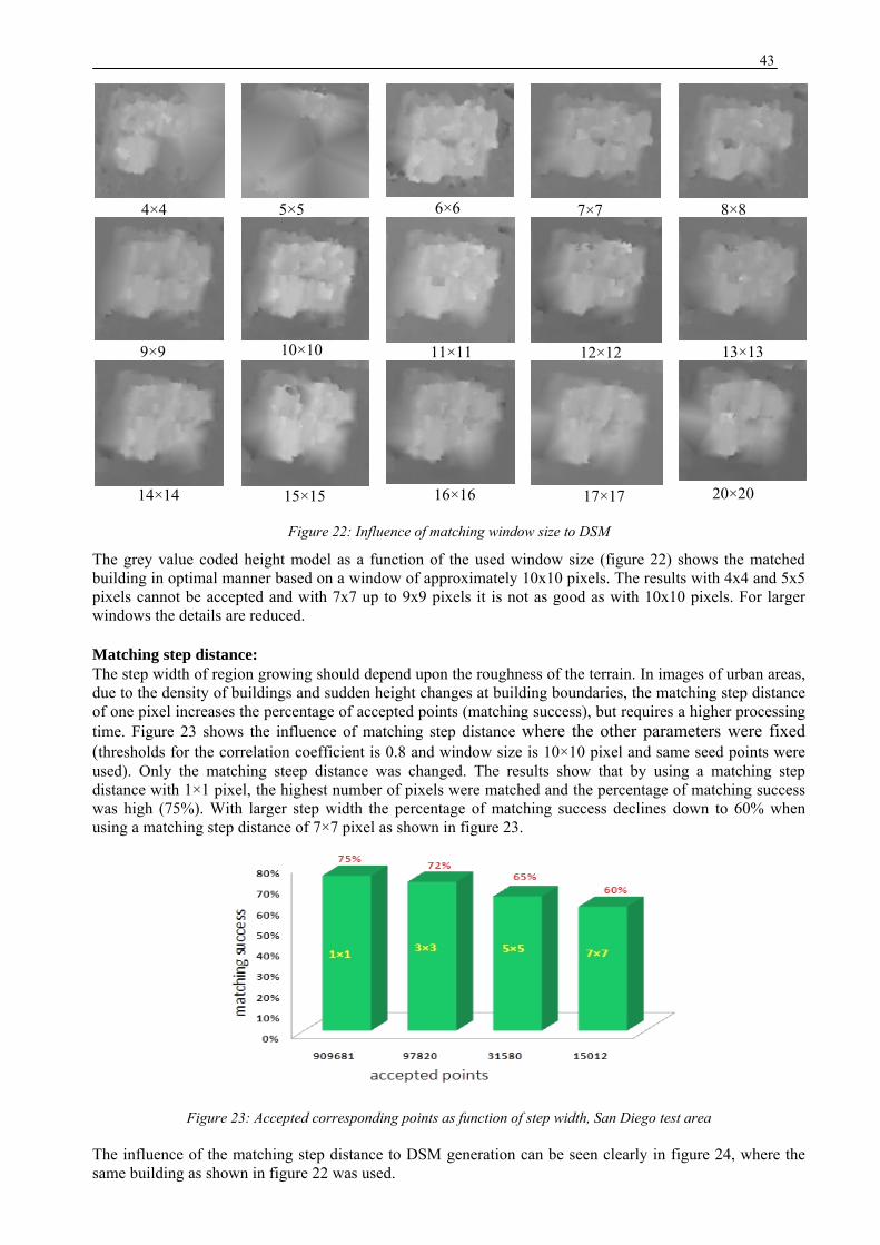
43

Figure 22: Influence of matching window size to DSM

The grey value coded height model as a function of the used window size (figure 22) shows the matched building in optimal manner based on a window of approximately 10x10 pixels. The results with 4x4 and 5x5 pixels cannot be accepted and with 7x7 up to 9x9 pixels it is not as good as with 10x10 pixels. For larger windows the details are reduced. Matching step distance: The step width of region growing should depend upon the roughness of the terrain. In images of urban areas, due to the density of buildings and sudden height changes at building boundaries, the matching step distance of one pixel increases the percentage of accepted points (matching success), but requires a higher processing time. Figure 23 shows the influence of matching step distance where the other parameters were fixed (thresholds for the correlation coefficient is 0.8 and window size is 10×10 pixel and same seed points were used). Only the matching steep distance was changed. The results show that by using a matching step distance with 1×1 pixel, the highest number of pixels were matched and the percentage of matching success was high (75%). With larger step width the percentage of matching success declines down to 60% when using a matching step distance of 7×7 pixel as shown in figure 23.

Figure 23: Accepted corresponding points as function of step width, San Diego test area

The influence of the matching step distance to DSM generation can be seen clearly in figure 24, where the same building as shown in figure 22 was used.

12×12

5×5 6×6 7×7 8×8

9×9 10×10 11×11

4×4

13×13

14×14 15×15 16×16 17×17 20×20

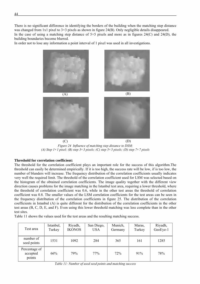
44

There is no significant difference in identifying the borders of the building when the matching step distance was changed from 1x1 pixel to 3×3 pixels as shown in figure 24(B). Only negligible details disappeared. In the case of using a matching step distance of 5×5 pixels and more as in figures 24(C) and 24(D), the building boundaries become blurred. In order not to lose any information a point interval of 1 pixel was used in all investigations.

Figure 24 Influence of matching step distance to DSM; (A) Step 1×1 pixel; (B) step 3×3 pixels; (C) step 5×5 pixels; (D) step 7×7 pixels

Threshold for correlation coefficient: The threshold for the correlation coefficient plays an important role for the success of this algorithm.The threshold can easily be determined empirically. If it is too high, the success rate will be low, if is too low, the number of blunders will increase. The frequency distribution of the correlation coefficients usually indicates very well the required limit. The threshold of the correlation coefficient used for LSM was selected based on the histogram of the obtained correlation coefficients. The image quality together with the different view direction causes problems for the image matching in the Istanbul test area, requiring a lower threshold, where the threshold of correlation coefficient was 0.6, while in the other test areas the threshold of correlation coefficient was 0.8. The smaller values of the LSM correlation coefficients for the test areas can be seen in the frequency distribution of the correlation coefficients in figure 25. The distribution of the correlation coefficients in Istanbul (A) is quite different for the distribution of the correlation coefficients in the other test areas (B, C, D, E, and F). Even using this lower threshold matching was less complete than in the other test sites. Table 11 shows the values used for the test areas and the resulting matching success.

Test area Istanbul, Turkey

Riyadh, IKONOS

San Diego, USA

Munich, Germany

Maras, Turkey

Riyadh, GeoEye-1

number of seed points 1531 1092 284 365 161 1285

Percentage of accepted

points 66% 79% 77% 72% 91% 78%

Table 11: Number of used seed points and matching success

(A) (B)

(C) (D)

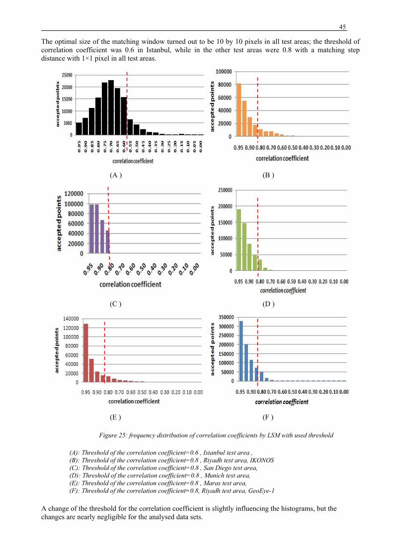
45

The optimal size of the matching window turned out to be 10 by 10 pixels in all test areas; the threshold of correlation coefficient was 0.6 in Istanbul, while in the other test areas were 0.8 with a matching step distance with 1×1 pixel in all test areas.

(A ) (B )

(C ) (D )

(E ) (F )

Figure 25: frequency distribution of correlation coefficients by LSM with used threshold

(A): Threshold of the correlation coefficient=0.6 , Istanbul test area , (B): Threshold of the correlation coefficient=0.8 , Riyadh test area, IKONOS (C): Threshold of the correlation coefficient=0.8 , San Diego test area, (D): Threshold of the correlation coefficient=0.8 , Munich test area, (E): Threshold of the correlation coefficient=0.8 , Maras test area, (F): Threshold of the correlation coefficient=0.8, Riyadh test area, GeoEye-1

A change of the threshold for the correlation coefficient is slightly influencing the histograms, but the changes are nearly negligible for the analysed data sets.

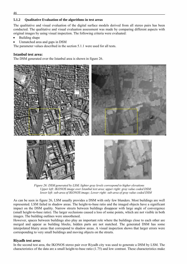
46

5.1.2 Qualitative Evaluation of the algorithms in test areas The qualitative and visual evaluation of the digital surface models derived from all stereo pairs has been conducted. The qualitative and visual evaluation assessment was made by comparing different aspects with original images by using visual inspection. The following criteria were evaluated: • Building shape • Unmatched area and gaps in DSM The parameter values described in the section 5.1.1 were used for all tests. Istanbul test area: The DSM generated over the Istanbul area is shown in figure 26.

Figure 26: DSM generated by LSM; lighter gray levels correspond to higher elevations Upper left: IKONOS image over Istanbul test area; upper right: gray value coded DSM; lower left: sub-area of IKONOS image; Lower right: sub-area of gray value coded DSM

As can be seen in figure 26, LSM usually provides a DSM with only few blunders. Most buildings are well represented. LSM failed in shadow areas. The height-to-base ratio and the imaged objects have a significant impact on the DSM quality. Narrow streets between buildings disappear with large angle of convergence (small height-to-base ratio). The larger occlusions caused a loss of some points, which are not visible in both images. The building outlines were smoothened. However, spaces between buildings also play an important role where the buildings close to each other are merged and appear as building blocks, hidden parts are not matched. The generated DSM has some interpolated blurry areas that correspond to shadow areas. A visual inspection shows that larger errors were corresponding to very small buildings and moving objects on the streets. Riyadh test area: In the second test area, the IKONOS stereo pair over Riyadh city was used to generate a DSM by LSM. The characteristics of the data are a small height-to-base ratio (1.75) and low contrast. These characteristics make

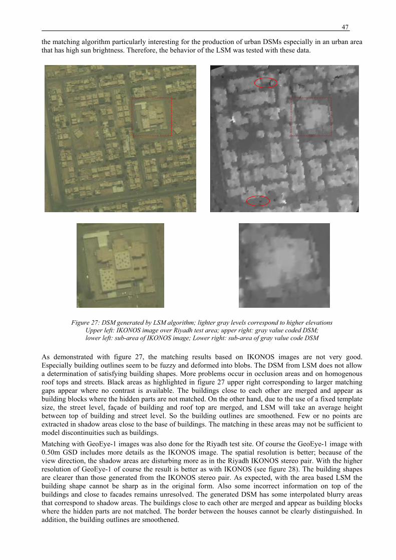
47

the matching algorithm particularly interesting for the production of urban DSMs especially in an urban area that has high sun brightness. Therefore, the behavior of the LSM was tested with these data.

Figure 27: DSM generated by LSM algorithm; lighter gray levels correspond to higher elevations Upper left: IKONOS image over Riyadh test area; upper right: gray value coded DSM; lower left: sub-area of IKONOS image; Lower right: sub-area of gray value code DSM

As demonstrated with figure 27, the matching results based on IKONOS images are not very good. Especially building outlines seem to be fuzzy and deformed into blobs. The DSM from LSM does not allow a determination of satisfying building shapes. More problems occur in occlusion areas and on homogenous roof tops and streets. Black areas as highlighted in figure 27 upper right corresponding to larger matching gaps appear where no contrast is available. The buildings close to each other are merged and appear as building blocks where the hidden parts are not matched. On the other hand, due to the use of a fixed template size, the street level, façade of building and roof top are merged, and LSM will take an average height between top of building and street level. So the building outlines are smoothened. Few or no points are extracted in shadow areas close to the base of buildings. The matching in these areas may not be sufficient to model discontinuities such as buildings. Matching with GeoEye-1 images was also done for the Riyadh test site. Of course the GeoEye-1 image with 0.50m GSD includes more details as the IKONOS image. The spatial resolution is better; because of the view direction, the shadow areas are disturbing more as in the Riyadh IKONOS stereo pair. With the higher resolution of GeoEye-1 of course the result is better as with IKONOS (see figure 28). The building shapes are clearer than those generated from the IKONOS stereo pair. As expected, with the area based LSM the building shape cannot be sharp as in the original form. Also some incorrect information on top of the buildings and close to facades remains unresolved. The generated DSM has some interpolated blurry areas that correspond to shadow areas. The buildings close to each other are merged and appear as building blocks where the hidden parts are not matched. The border between the houses cannot be clearly distinguished. In addition, the building outlines are smoothened.

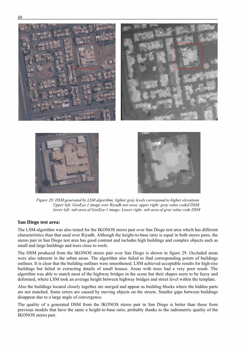
48

Figure 28: DSM generated by LSM algorithm; lighter gray levels correspond to higher elevations Upper left: GeoEye-1 image over Riyadh test area; upper right: gray value coded DSM; lower left: sub-area of GeoEye-1 image; Lower right: sub-area of gray value code DSM

San Diego test area: The LSM-algorithm was also tested for the IKONOS stereo pair over San Diego test area which has different characteristics than that used over Riyadh. Although the height-to-base ratio is equal in both stereo pairs, the stereo pair in San Diego test area has good contrast and includes high buildings and complex objects such as small and large buildings and trees close to roofs. The DSM produced from the IKONOS stereo pair over San Diego is shown in figure 29. Occluded areas were also inherent in the urban areas. The algorithm also failed to find corresponding points of buildings outlines. It is clear that the building outlines were smoothened. LSM achieved acceptable results for high-rise buildings but failed in extracting details of small houses. Areas with trees had a very poor result. The algorithm was able to match most of the highway bridges in the scene but their shapes seem to be fuzzy and deformed, where LSM took an average height between highway bridges and street level within the template. Also the buildings located closely together are merged and appear as building blocks where the hidden parts are not matched. Some errors are caused by moving objects on the streets. Smaller gaps between buildings disappear due to a large angle of convergence. The quality of a generated DSM from the IKONOS stereo pair in San Diego is better than those from previous models that have the same a height-to-base ratio, probably thanks to the radiometric quality of the IKONOS stereo pair.

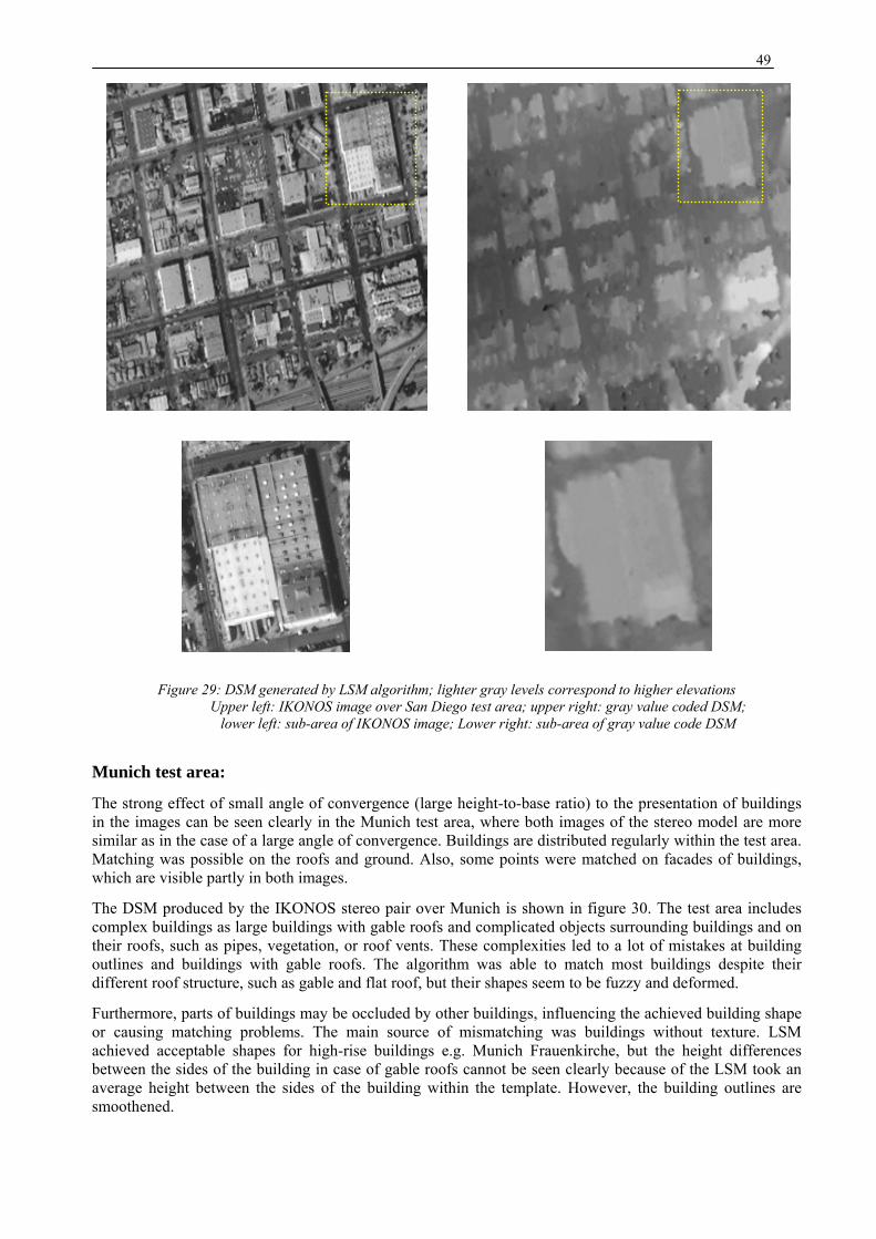
49

Figure 29: DSM generated by LSM algorithm; lighter gray levels correspond to higher elevations Upper left: IKONOS image over San Diego test area; upper right: gray value coded DSM;

lower left: sub-area of IKONOS image; Lower right: sub-area of gray value code DSM

Munich test area:

The strong effect of small angle of convergence (large height-to-base ratio) to the presentation of buildings in the images can be seen clearly in the Munich test area, where both images of the stereo model are more similar as in the case of a large angle of convergence. Buildings are distributed regularly within the test area. Matching was possible on the roofs and ground. Also, some points were matched on facades of buildings, which are visible partly in both images.

The DSM produced by the IKONOS stereo pair over Munich is shown in figure 30. The test area includes complex buildings as large buildings with gable roofs and complicated objects surrounding buildings and on their roofs, such as pipes, vegetation, or roof vents. These complexities led to a lot of mistakes at building outlines and buildings with gable roofs. The algorithm was able to match most buildings despite their different roof structure, such as gable and flat roof, but their shapes seem to be fuzzy and deformed.

Furthermore, parts of buildings may be occluded by other buildings, influencing the achieved building shape or causing matching problems. The main source of mismatching was buildings without texture. LSM achieved acceptable shapes for high-rise buildings e.g. Munich Frauenkirche, but the height differences between the sides of the building in case of gable roofs cannot be seen clearly because of the LSM took an average height between the sides of the building within the template. However, the building outlines are smoothened.

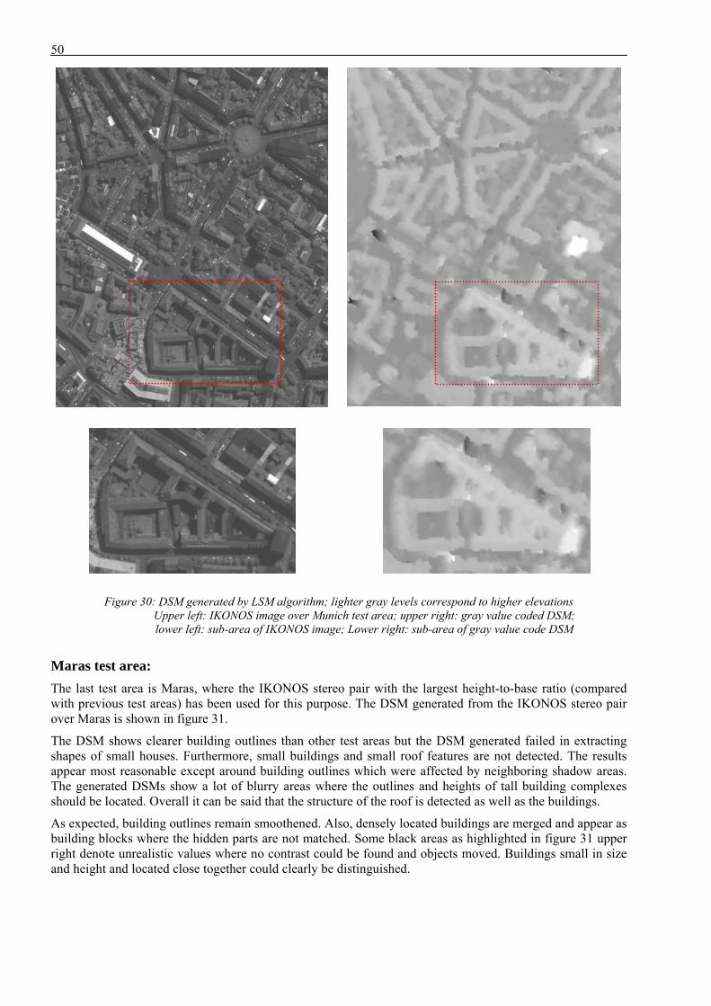
50

Figure 30: DSM generated by LSM algorithm; lighter gray levels correspond to higher elevations Upper left: IKONOS image over Munich test area; upper right: gray value coded DSM; lower left: sub-area of IKONOS image; Lower right: sub-area of gray value code DSM

Maras test area: The last test area is Maras, where the IKONOS stereo pair with the largest height-to-base ratio (compared with previous test areas) has been used for this purpose. The DSM generated from the IKONOS stereo pair over Maras is shown in figure 31.

The DSM shows clearer building outlines than other test areas but the DSM generated failed in extracting shapes of small houses. Furthermore, small buildings and small roof features are not detected. The results appear most reasonable except around building outlines which were affected by neighboring shadow areas. The generated DSMs show a lot of blurry areas where the outlines and heights of tall building complexes should be located. Overall it can be said that the structure of the roof is detected as well as the buildings.

As expected, building outlines remain smoothened. Also, densely located buildings are merged and appear as building blocks where the hidden parts are not matched. Some black areas as highlighted in figure 31 upper right denote unrealistic values where no contrast could be found and objects moved. Buildings small in size and height and located close together could clearly be distinguished.

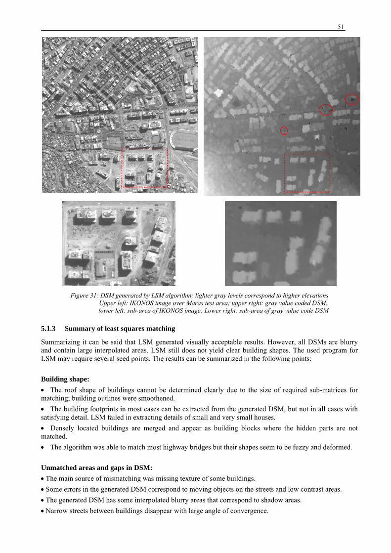
51

Figure 31: DSM generated by LSM algorithm; lighter gray levels correspond to higher elevations

Upper left: IKONOS image over Maras test area; upper right: gray value coded DSM; lower left: sub-area of IKONOS image; Lower right: sub-area of gray value code DSM

5.1.3 Summary of least squares matching

Summarizing it can be said that LSM generated visually acceptable results. However, all DSMs are blurry and contain large interpolated areas. LSM still does not yield clear building shapes. The used program for LSM may require several seed points. The results can be summarized in the following points: Building shape: • The roof shape of buildings cannot be determined clearly due to the size of required sub-matrices for matching; building outlines were smoothened. • The building footprints in most cases can be extracted from the generated DSM, but not in all cases with satisfying detail. LSM failed in extracting details of small and very small houses. • Densely located buildings are merged and appear as building blocks where the hidden parts are not matched. • The algorithm was able to match most highway bridges but their shapes seem to be fuzzy and deformed. Unmatched areas and gaps in DSM: • The main source of mismatching was missing texture of some buildings. • Some errors in the generated DSM correspond to moving objects on the streets and low contrast areas. • The generated DSM has some interpolated blurry areas that correspond to shadow areas. • Narrow streets between buildings disappear with large angle of convergence.

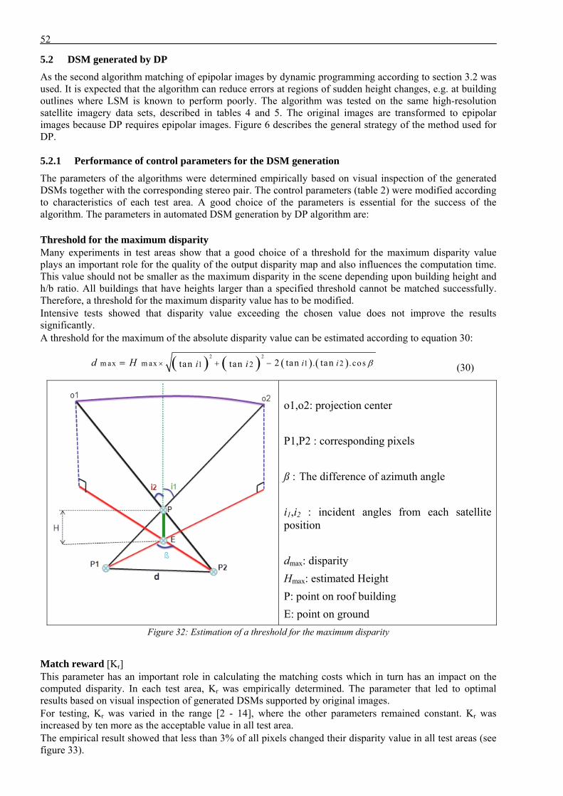
52

5.2 DSM generated by DP

As the second algorithm matching of epipolar images by dynamic programming according to section 3.2 was used. It is expected that the algorithm can reduce errors at regions of sudden height changes, e.g. at building outlines where LSM is known to perform poorly. The algorithm was tested on the same high-resolution satellite imagery data sets, described in tables 4 and 5. The original images are transformed to epipolar images because DP requires epipolar images. Figure 6 describes the general strategy of the method used for DP.

5.2.1 Performance of control parameters for the DSM generation

The parameters of the algorithms were determined empirically based on visual inspection of the generated DSMs together with the corresponding stereo pair. The control parameters (table 2) were modified according to characteristics of each test area. A good choice of the parameters is essential for the success of the algorithm. The parameters in automated DSM generation by DP algorithm are: Threshold for the maximum disparity Many experiments in test areas show that a good choice of a threshold for the maximum disparity value plays an important role for the quality of the output disparity map and also influences the computation time. This value should not be smaller as the maximum disparity in the scene depending upon building height and h/b ratio. All buildings that have heights larger than a specified threshold cannot be matched successfully. Therefore, a threshold for the maximum disparity value has to be modified. Intensive tests showed that disparity value exceeding the chosen value does not improve the results significantly. A threshold for the maximum of the absolute disparity value can be estimated according to equation 30:

( ) ( ) ( ) ( )2 2

m ax m ax 1 21 2 . . cos2 tan tantan tan i ii id H β× + −= (30)

o1,o2: projection center P1,P2 : corresponding pixels ß : The difference of azimuth angle i1,i2 : incident angles from each satellite position dmax: disparity Hmax: estimated Height P: point on roof building E: point on ground

Figure 32: Estimation of a threshold for the maximum disparity

Match reward [Kr] This parameter has an important role in calculating the matching costs which in turn has an impact on the computed disparity. In each test area, Kr was empirically determined. The parameter that led to optimal results based on visual inspection of generated DSMs supported by original images. For testing, Kr was varied in the range [2 - 14], where the other parameters remained constant. Kr was increased by ten more as the acceptable value in all test area. The empirical result showed that less than 3% of all pixels changed their disparity value in all test areas (see figure 33).

53

Figure 33: Match reward values with percentage of changed disparity values against results achieved with Kr = 2; IKONOS Riyadh teat area

The tests showed that only the building shapes were influenced by increased Kr but the building heights were not affected when Kr was increased above the acceptable value in each test area, where the heights of ten buildings were compared with reference data. In addition, changed values were outside the stereoscopic coverage, where only one image was available. Some changes in few building outlines occurred. The acceptable values of Kr in test areas summarized in the table 12:

Test area Istanbul Riyadh, IKONOS San Diego Munich Maras Riyadh,

GeoEye-1

Kr

7 7 7 14 7 7

Table 12: Selected values of Kr in test areas

Penalty for occlusions [Kocc] As mentioned in section 3.2.5, changes in height and occlusions in the urban area are visible as intensity changes. Kocc is sensitive to intensity values of corresponding pixels. Each change in height incurs an occlusion penalty. For this reason the values of Kocc have to be increased in areas containing large occlusions. Kocc was varied up to reaching an acceptable disparity image in each test area. Kocc was varied in the range [4 - 21], where the other parameters remained constant. The tests show that less than 9% of all pixels changed their disparity value when Kocc was increased by ten more as the acceptable value of Kocc. Figure 34 shows the percentage of changed disparity values depending upon Kocc. The selected value of Kocc is 4.

Figure 34: Influence of penalty for occlusions to disparity value changes; IKONOS Riyadh teat area

The algorithm imposes a penalty on each occlusion rather than for each occluded pixel, therefore, by increasing Kocc above the acceptable value more than ten above the acceptable value, the shapes of the buildings are affected. At locations were buildings are close to each other objects with similar heights can merge.

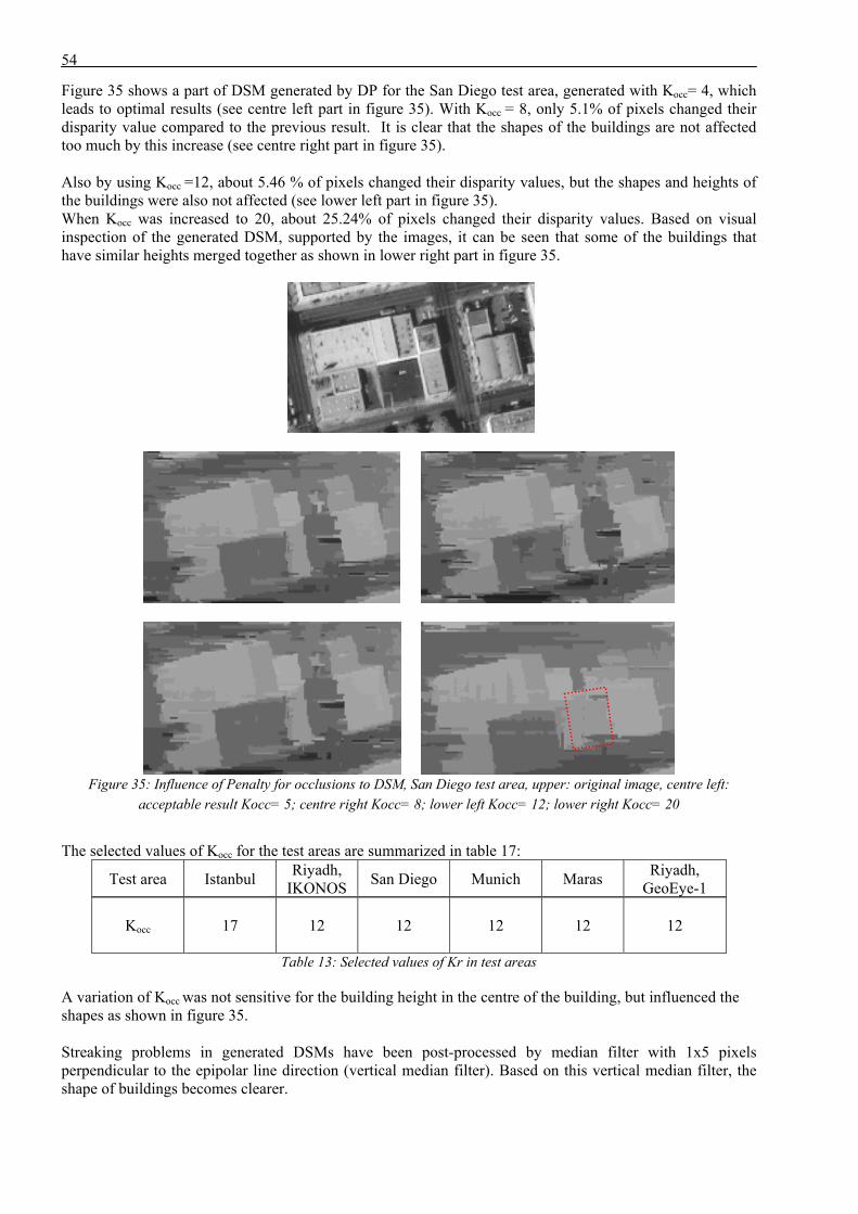
54

Figure 35 shows a part of DSM generated by DP for the San Diego test area, generated with Kocc= 4, which leads to optimal results (see centre left part in figure 35). With Kocc = 8, only 5.1% of pixels changed their disparity value compared to the previous result. It is clear that the shapes of the buildings are not affected too much by this increase (see centre right part in figure 35). Also by using Kocc =12, about 5.46 % of pixels changed their disparity values, but the shapes and heights of the buildings were also not affected (see lower left part in figure 35). When Kocc was increased to 20, about 25.24% of pixels changed their disparity values. Based on visual inspection of the generated DSM, supported by the images, it can be seen that some of the buildings that have similar heights merged together as shown in lower right part in figure 35.

Figure 35: Influence of Penalty for occlusions to DSM, San Diego test area, upper: original image, centre left:

acceptable result Kocc= 5; centre right Kocc= 8; lower left Kocc= 12; lower right Kocc= 20

The selected values of Kocc for the test areas are summarized in table 17:

Test area Istanbul Riyadh, IKONOS San Diego Munich Maras Riyadh,

GeoEye-1

Kocc

17 12 12 12 12 12

Table 13: Selected values of Kr in test areas

A variation of Kocc was not sensitive for the building height in the centre of the building, but influenced the shapes as shown in figure 35. Streaking problems in generated DSMs have been post-processed by median filter with 1x5 pixels perpendicular to the epipolar line direction (vertical median filter). Based on this vertical median filter, the shape of buildings becomes clearer.

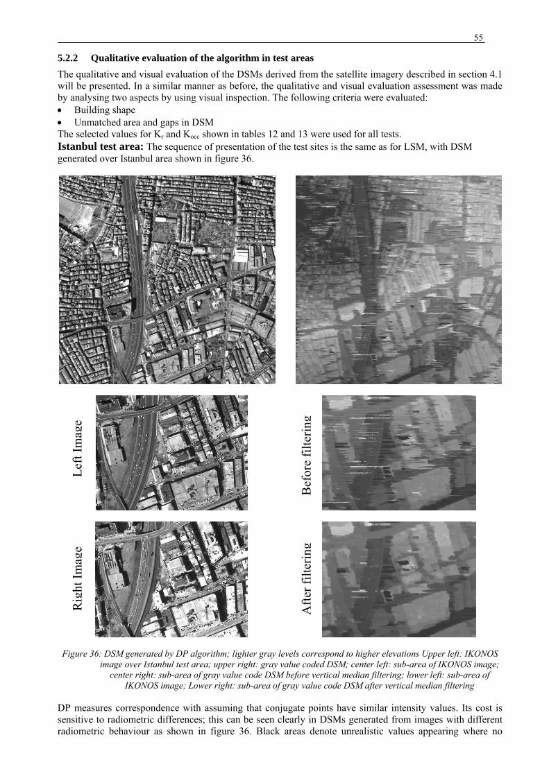
55

5.2.2 Qualitative evaluation of the algorithm in test areas The qualitative and visual evaluation of the DSMs derived from the satellite imagery described in section 4.1 will be presented. In a similar manner as before, the qualitative and visual evaluation assessment was made by analysing two aspects by using visual inspection. The following criteria were evaluated: • Building shape • Unmatched area and gaps in DSM The selected values for Kr and Kocc shown in tables 12 and 13 were used for all tests. Istanbul test area: The sequence of presentation of the test sites is the same as for LSM, with DSM generated over Istanbul area shown in figure 36.

Figure 36: DSM generated by DP algorithm; lighter gray levels correspond to higher elevations Upper left: IKONOS image over Istanbul test area; upper right: gray value coded DSM; center left: sub-area of IKONOS image;

center right: sub-area of gray value code DSM before vertical median filtering; lower left: sub-area of IKONOS image; Lower right: sub-area of gray value code DSM after vertical median filtering

DP measures correspondence with assuming that conjugate points have similar intensity values. Its cost is sensitive to radiometric differences; this can be seen clearly in DSMs generated from images with different radiometric behaviour as shown in figure 36. Black areas denote unrealistic values appearing where no

Left

Imag

e R

ight

Imag

e

Bef

ore

filte

ring

Afte

r filt

erin

g

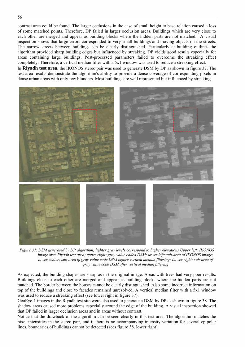
56

contrast area could be found. The larger occlusions in the case of small height to base relation caused a loss of some matched points. Therefore, DP failed in larger occlusion areas. Buildings which are very close to each other are merged and appear as building blocks where the hidden parts are not matched. A visual inspection shows that large errors corresponded to very small buildings and moving objects on the streets. The narrow streets between buildings can be clearly distinguished. Particularly at building outlines the algorithm provided sharp building edges but influenced by streaking. DP yields good results especially for areas containing large buildings. Post-processed parameters failed to overcome the streaking effect completely. Therefore, a vertical median filter with a 5x1 window was used to reduce a streaking effect. In Riyadh test area, the IKONOS stereo pair was used to generate DSM by DP as shown in figure 37. The test area results demonstrate the algorithm's ability to provide a dense coverage of corresponding pixels in dense urban areas with only few blunders. Most buildings are well represented but influenced by streaking.

Figure 37: DSM generated by DP algorithm; lighter gray levels correspond to higher elevations Upper left: IKONOS

image over Riyadh test area; upper right: gray value coded DSM; lower left: sub-area of IKONOS image; lower center: sub-area of gray value code DSM before vertical median filtering; Lower right: sub-area of

gray value code DSM after vertical median filtering

As expected, the building shapes are sharp as in the original image. Areas with trees had very poor results. Buildings close to each other are merged and appear as building blocks where the hidden parts are not matched. The border between the houses cannot be clearly distinguished. Also some incorrect information on top of the buildings and close to facades remained unresolved. A vertical median filter with a 5x1 window was used to reduce a streaking effect (see lower right in figure 37). GeoEye-1 images in the Riyadh test site were also used to generate a DSM by DP as shown in figure 38. The shadow areas caused more problems especially around the edge of the building. A visual inspection showed that DP failed in larger occlusion areas and in areas without contrast. Notice that the drawback of the algorithm can be seen clearly in this test area. The algorithm matches the pixel intensities in the stereo pair, and if there is no accompanying intensity variation for several epipolar lines, boundaries of buildings cannot be detected (sees figure 38, lower right)

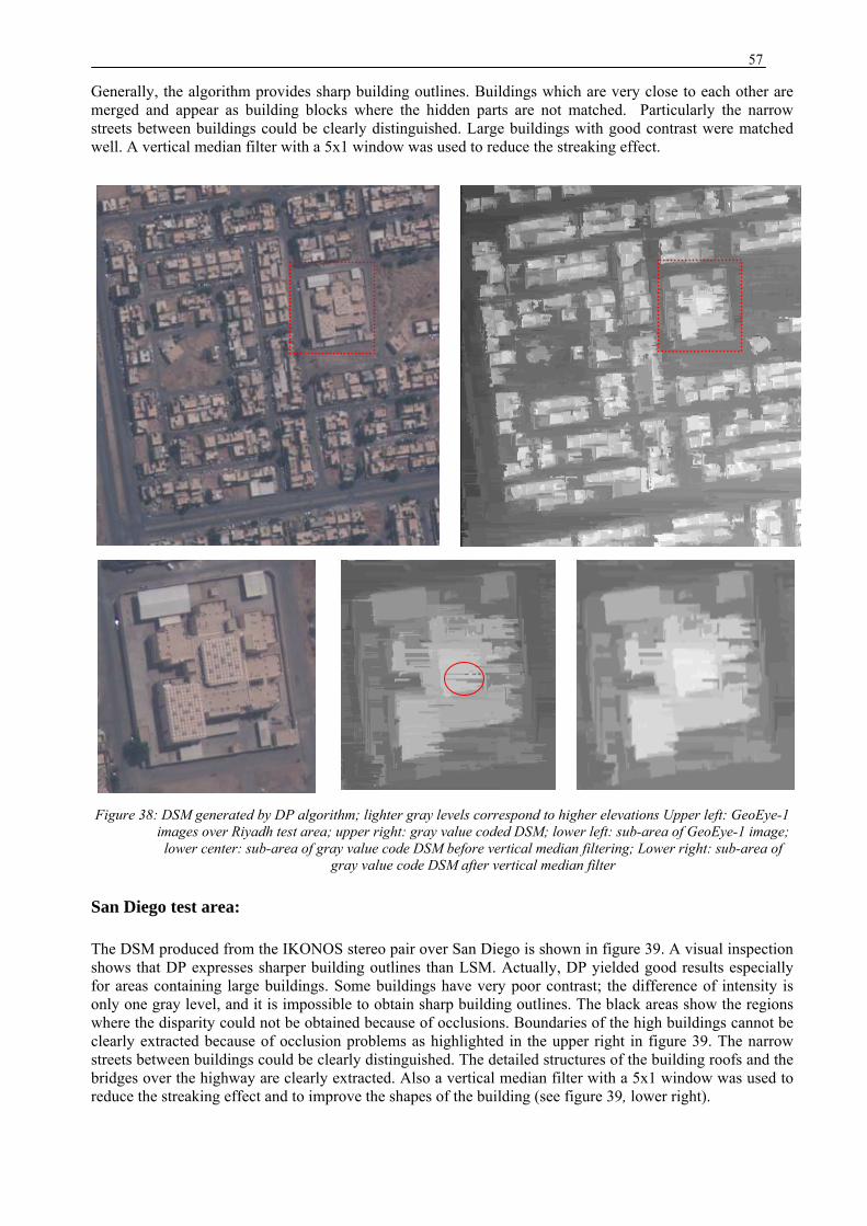
57

Generally, the algorithm provides sharp building outlines. Buildings which are very close to each other are merged and appear as building blocks where the hidden parts are not matched. Particularly the narrow streets between buildings could be clearly distinguished. Large buildings with good contrast were matched well. A vertical median filter with a 5x1 window was used to reduce the streaking effect.

Figure 38: DSM generated by DP algorithm; lighter gray levels correspond to higher elevations Upper left: GeoEye-1 images over Riyadh test area; upper right: gray value coded DSM; lower left: sub-area of GeoEye-1 image; lower center: sub-area of gray value code DSM before vertical median filtering; Lower right: sub-area of

gray value code DSM after vertical median filter

San Diego test area:

The DSM produced from the IKONOS stereo pair over San Diego is shown in figure 39. A visual inspection shows that DP expresses sharper building outlines than LSM. Actually, DP yielded good results especially for areas containing large buildings. Some buildings have very poor contrast; the difference of intensity is only one gray level, and it is impossible to obtain sharp building outlines. The black areas show the regions where the disparity could not be obtained because of occlusions. Boundaries of the high buildings cannot be clearly extracted because of occlusion problems as highlighted in the upper right in figure 39. The narrow streets between buildings could be clearly distinguished. The detailed structures of the building roofs and the bridges over the highway are clearly extracted. Also a vertical median filter with a 5x1 window was used to reduce the streaking effect and to improve the shapes of the building (see figure 39, lower right).

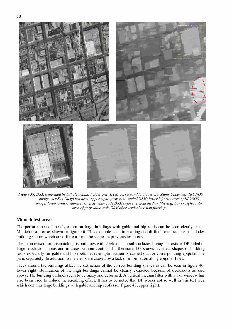
58

Figure 39: DSM generated by DP algorithm; lighter gray levels correspond to higher elevations Upper left: IKONOS image over San Diego test area; upper right: gray value coded DSM; lower left: sub-area of IKONOS

image; lower center: sub-area of gray value code DSM before vertical median filtering; Lower right: sub-area of gray value code DSM after vertical median filtering

Munich test area: The performance of the algorithm on large buildings with gable and hip roofs can be seen clearly in the Munich test area as shown in figure 40. This example is an interesting and difficult one because it includes building shapes which are different from the shapes in previous test areas. The main reason for mismatching is buildings with sleek and smooth surfaces having no texture. DP failed in larger occlusions areas and in areas without contrast. Furthermore, DP shows incorrect shapes of building roofs especially for gable and hip roofs because optimization is carried out for corresponding epipolar line pairs separately. In addition, some errors are caused by a lack of information along epipolar lines. Trees around the buildings affect the extraction of the correct building shapes as can be seen in figure 40, lower right. Boundaries of the high buildings cannot be clearly extracted because of occlusions as said above. The building outlines seem to be fuzzy and deformed. A vertical median filter with a 5x1 window has also been used to reduce the streaking effect. It has to be noted that DP works not so well in this test area which contains large buildings with gable and hip roofs (see figure 40, upper right).

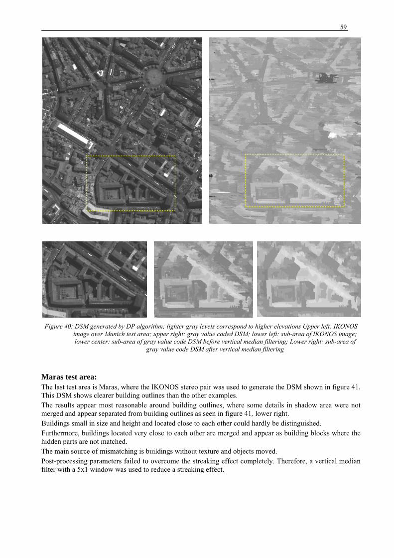
59

Figure 40: DSM generated by DP algorithm; lighter gray levels correspond to higher elevations Upper left: IKONOS

image over Munich test area; upper right: gray value coded DSM; lower left: sub-area of IKONOS image; lower center: sub-area of gray value code DSM before vertical median filtering; Lower right: sub-area of

gray value code DSM after vertical median filtering

Maras test area: The last test area is Maras, where the IKONOS stereo pair was used to generate the DSM shown in figure 41. This DSM shows clearer building outlines than the other examples. The results appear most reasonable around building outlines, where some details in shadow area were not merged and appear separated from building outlines as seen in figure 41, lower right. Buildings small in size and height and located close to each other could hardly be distinguished. Furthermore, buildings located very close to each other are merged and appear as building blocks where the hidden parts are not matched. The main source of mismatching is buildings without texture and objects moved. Post-processing parameters failed to overcome the streaking effect completely. Therefore, a vertical median filter with a 5x1 window was used to reduce a streaking effect.

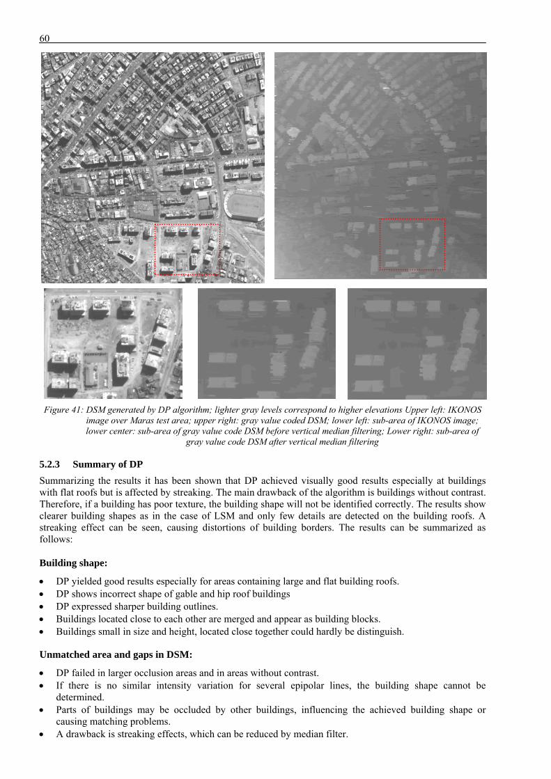
60

Figure 41: DSM generated by DP algorithm; lighter gray levels correspond to higher elevations Upper left: IKONOS

image over Maras test area; upper right: gray value coded DSM; lower left: sub-area of IKONOS image; lower center: sub-area of gray value code DSM before vertical median filtering; Lower right: sub-area of

gray value code DSM after vertical median filtering

5.2.3 Summary of DP Summarizing the results it has been shown that DP achieved visually good results especially at buildings with flat roofs but is affected by streaking. The main drawback of the algorithm is buildings without contrast. Therefore, if a building has poor texture, the building shape will not be identified correctly. The results show clearer building shapes as in the case of LSM and only few details are detected on the building roofs. A streaking effect can be seen, causing distortions of building borders. The results can be summarized as follows: Building shape:

• DP yielded good results especially for areas containing large and flat building roofs. • DP shows incorrect shape of gable and hip roof buildings • DP expressed sharper building outlines. • Buildings located close to each other are merged and appear as building blocks. • Buildings small in size and height, located close together could hardly be distinguish.

Unmatched area and gaps in DSM:

• DP failed in larger occlusion areas and in areas without contrast. • If there is no similar intensity variation for several epipolar lines, the building shape cannot be

determined. • Parts of buildings may be occluded by other buildings, influencing the achieved building shape or

causing matching problems. • A drawback is streaking effects, which can be reduced by median filter.

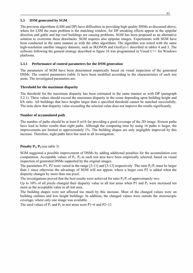
61

5.3 DSM generated by SGM

The previous algorithms (LSM and DP) have difficulties in providing high quality DSMs as discussed above, where for LSM the main problem is the matching window, for DP streaking effects appear in the epipolar direction and gable and hip roof buildings are causing problems. SGM has been proposed as an alternative solution to overcome these drawbacks. SGM requires also epipolar images. Experiments with SGM have been conducted in the same manner as with the other algorithms. The algorithm was tested with the same high-resolution satellite imagery datasets, such as IKONOS and GeoEye-1 described in tables 4 and 5. The software following the general strategy described in figure 10 was programmed in Visual C++ for Windows platforms.

5.3.1 Performance of control parameters for the DSM generation

The parameters of SGM have been determined empirically based on visual inspection of the generated DSMs. The control parameters (table 3) have been modified according to the characteristics of each test areas. The investigated parameters are:

Threshold for the maximum disparity

The threshold for the maximum disparity has been estimated in the same manner as with DP (paragraph 5.2.1). These values should exceed the maximum disparity in the scene depending upon building height and h/b ratio. All buildings that have heights larger than a specified threshold cannot be matched successfully. The tests show that disparity value exceeding the selected value does not improve the results significantly. Number of accumulated path

The number of paths should be at least 8 or16 for providing a good coverage of the 2D image. Sixteen paths have lead to better results than eight paths. Although the computing time by using 16 paths is larger, the improvements are limited to approximately 1%. The building shapes are only negligible improved by this increase. Therefore, eight paths have bee used in all investigation.

Penalty P1, P2 (see table 3)

SGM suggested a possible improvement of DSMs by adding additional penalties for the accumulation cost computation. Acceptable values of P1, P2 in each test area have been empirically selected, based on visual inspection of generated DSMs supported by the original images. The parameters P1, P2 were varied in the range [3-11] and [3-13] respectively .The ratio P2/P1 must be larger than 1 since otherwise the advantage of SGM will not appear, where a larger cost P2 is added when the disparity changes by more than one pixel. The investigations proved that the best results were achieved for ratio P2/P1 of approximately two. Up to 10% of all pixels changed their disparity value in all test areas when P1 and P2 were increased ten more as the acceptable value in all test area. The building shapes were not affected too much by this increase. Most of the changed values were on building outlines and low height buildings. In addition, the changed values were outside the stereoscopic coverage, where only one image was available. The used values of P1 and P2 in test areas were P1=6 and P2=12

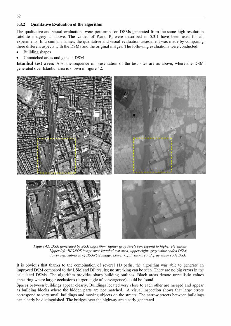
62

5.3.2 Qualitative Evaluation of the algorithm

The qualitative and visual evaluations were performed on DSMs generated from the same high-resolution satellite imagery as above. The values of P1and P2 were described in 5.3.1 have been used for all experiments. In a similar manner, the qualitative and visual evaluation assessment was made by comparing three different aspects with the DSMs and the original images. The following evaluations were conducted: • Building shapes • Unmatched areas and gaps in DSM Istanbul test area: Also the sequence of presentation of the test sites are as above, where the DSM generated over Istanbul area is shown in figure 42.

Figure 42: DSM generated by SGM algorithm; lighter gray levels correspond to higher elevations Upper left: IKONOS image over Istanbul test area; upper right: gray value coded DSM; lower left: sub-area of IKONOS image; Lower right: sub-area of gray value code DSM

It is obvious that thanks to the combination of several 1D paths, the algorithm was able to generate an improved DSM compared to the LSM and DP results; no streaking can be seen. There are no big errors in the calculated DSMs. The algorithm provides sharp building outlines. Black areas denote unrealistic values appearing where larger occlusions (larger angle of convergence) could be found. Spaces between buildings appear clearly. Buildings located very close to each other are merged and appear as building blocks where the hidden parts are not matched. A visual inspection shows that large errors correspond to very small buildings and moving objects on the streets. The narrow streets between buildings can clearly be distinguished. The bridges over the highway are clearly generated.

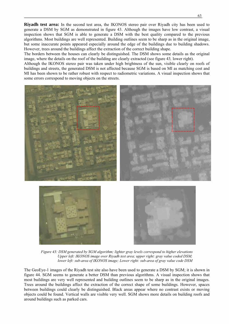
63

Riyadh test area: In the second test area, the IKONOS stereo pair over Riyadh city has been used to generate a DSM by SGM as demonstrated in figure 43. Although the images have low contrast, a visual inspection shows that SGM is able to generate a DSM with the best quality compared to the previous algorithms. Most buildings are well represented. Building outlines seem to be sharp as in the original image, but some inaccurate points appeared especially around the edge of the buildings due to building shadows. However, trees around the buildings affect the extraction of the correct building shape. The borders between the houses can clearly be distinguished. The DSM shows some details as the original image, where the details on the roof of the building are clearly extracted (see figure 43, lower right). Although the IKONOS stereo pair was taken under high brightness of the sun, visible clearly on roofs of buildings and streets, the generated DSM is not affected because SGM is based on MI as matching cost and MI has been shown to be rather robust with respect to radiometric variations. A visual inspection shows that some errors correspond to moving objects on the streets.

Figure 43: DSM generated by SGM algorithm; lighter gray levels correspond to higher elevations Upper left: IKONOS image over Riyadh test area; upper right: gray value coded DSM; lower left: sub-area of IKONOS image; Lower right: sub-area of gray value code DSM

The GeoEye-1 images of the Riyadh test site also have been used to generate a DSM by SGM; it is shown in figure 44. SGM seems to generate a better DSM than previous algorithms. A visual inspection shows that most buildings are very well represented and building outlines seem to be sharp as in the original images. Trees around the buildings affect the extraction of the correct shape of some buildings. However, spaces between buildings could clearly be distinguished. Black areas appear where no contrast exists or moving objects could be found. Vertical walls are visible very well. SGM shows more details on building roofs and around buildings such as parked cars.

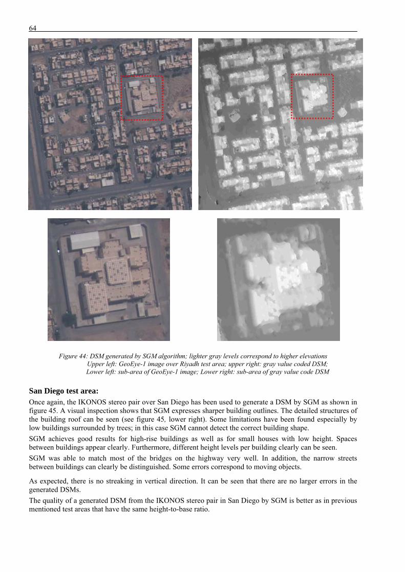
64

Figure 44: DSM generated by SGM algorithm; lighter gray levels correspond to higher elevations Upper left: GeoEye-1 image over Riyadh test area; upper right: gray value coded DSM; Lower left: sub-area of GeoEye-1 image; Lower right: sub-area of gray value code DSM

San Diego test area: Once again, the IKONOS stereo pair over San Diego has been used to generate a DSM by SGM as shown in figure 45. A visual inspection shows that SGM expresses sharper building outlines. The detailed structures of the building roof can be seen (see figure 45, lower right). Some limitations have been found especially by low buildings surrounded by trees; in this case SGM cannot detect the correct building shape. SGM achieves good results for high-rise buildings as well as for small houses with low height. Spaces between buildings appear clearly. Furthermore, different height levels per building clearly can be seen. SGM was able to match most of the bridges on the highway very well. In addition, the narrow streets between buildings can clearly be distinguished. Some errors correspond to moving objects.

As expected, there is no streaking in vertical direction. It can be seen that there are no larger errors in the generated DSMs. The quality of a generated DSM from the IKONOS stereo pair in San Diego by SGM is better as in previous mentioned test areas that have the same height-to-base ratio.

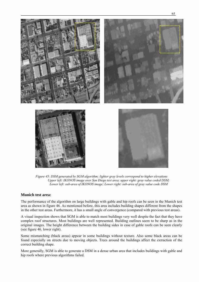
65

Figure 45: DSM generated by SGM algorithm; lighter gray levels correspond to higher elevations Upper left: IKONOS image over San Diego test area; upper right: gray value coded DSM;

Lower left: sub-area of IKONOS image; Lower right: sub-area of gray value code DSM

Munich test area: The performance of the algorithm on large buildings with gable and hip roofs can be seen in the Munich test area as shown in figure 46. As mentioned before, this area includes building shapes different from the shapes in the other test areas. Furthermore, it has a small angle of convergence (compared with previous test areas).

A visual inspection shows that SGM is able to match most buildings very well despite the fact that they have complex roof structures. Most buildings are well represented. Building outlines seem to be sharp as in the original images. The height difference between the building sides in case of gable roofs can be seen clearly (see figure 46, lower right).

Some mismatching (black areas) appear in some buildings without texture. Also some black areas can be found especially on streets due to moving objects. Trees around the buildings affect the extraction of the correct building shape.

More generally, SGM is able to generate a DSM in a dense urban area that includes buildings with gable and hip roofs where previous algorithms failed.

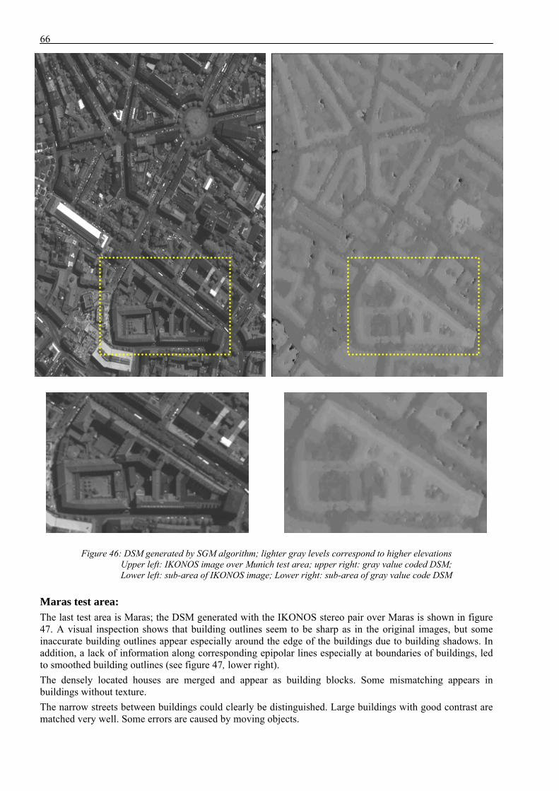
66

Figure 46: DSM generated by SGM algorithm; lighter gray levels correspond to higher elevations Upper left: IKONOS image over Munich test area; upper right: gray value coded DSM; Lower left: sub-area of IKONOS image; Lower right: sub-area of gray value code DSM

Maras test area: The last test area is Maras; the DSM generated with the IKONOS stereo pair over Maras is shown in figure 47. A visual inspection shows that building outlines seem to be sharp as in the original images, but some inaccurate building outlines appear especially around the edge of the buildings due to building shadows. In addition, a lack of information along corresponding epipolar lines especially at boundaries of buildings, led to smoothed building outlines (see figure 47, lower right). The densely located houses are merged and appear as building blocks. Some mismatching appears in buildings without texture. The narrow streets between buildings could clearly be distinguished. Large buildings with good contrast are matched very well. Some errors are caused by moving objects.

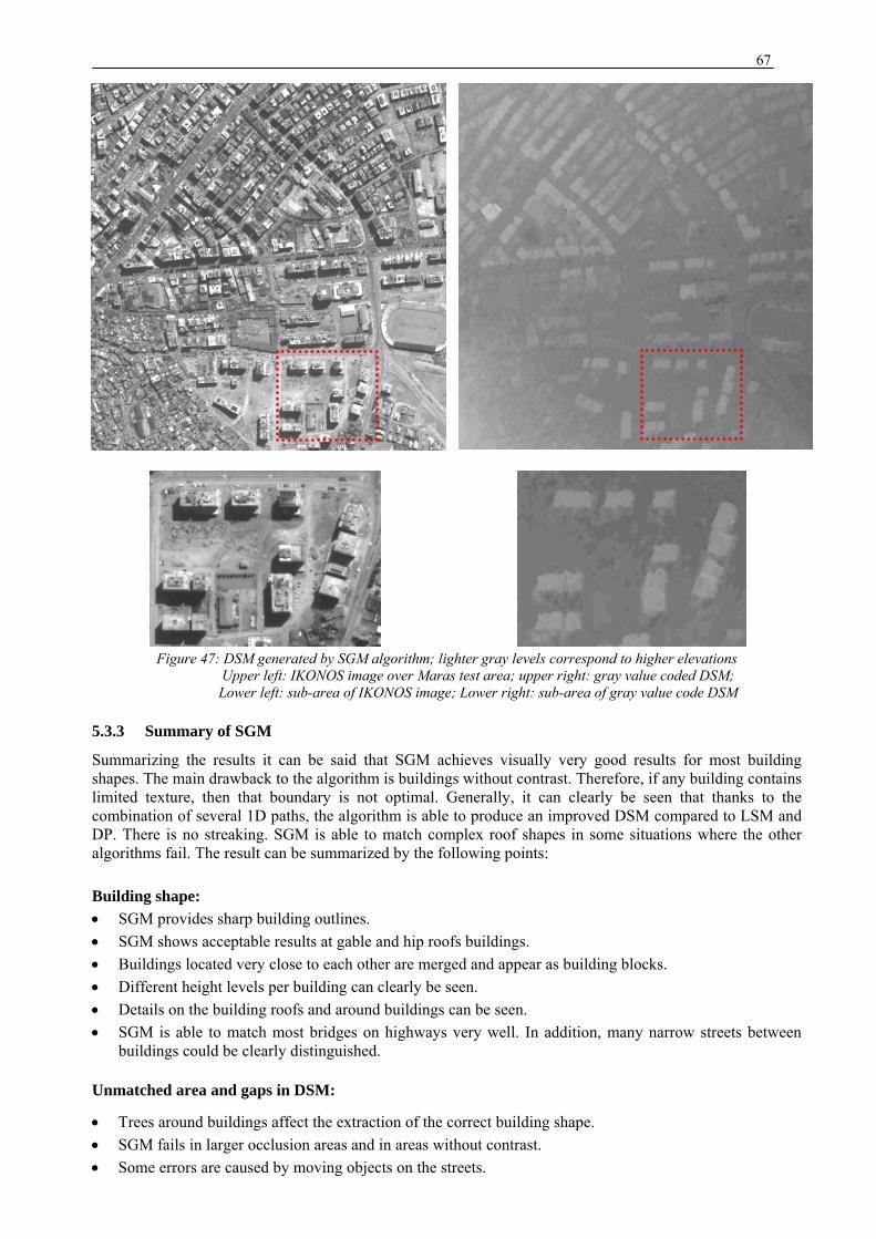
67

Figure 47: DSM generated by SGM algorithm; lighter gray levels correspond to higher elevations Upper left: IKONOS image over Maras test area; upper right: gray value coded DSM; Lower left: sub-area of IKONOS image; Lower right: sub-area of gray value code DSM

5.3.3 Summary of SGM

Summarizing the results it can be said that SGM achieves visually very good results for most building shapes. The main drawback to the algorithm is buildings without contrast. Therefore, if any building contains limited texture, then that boundary is not optimal. Generally, it can clearly be seen that thanks to the combination of several 1D paths, the algorithm is able to produce an improved DSM compared to LSM and DP. There is no streaking. SGM is able to match complex roof shapes in some situations where the other algorithms fail. The result can be summarized by the following points: Building shape: • SGM provides sharp building outlines. • SGM shows acceptable results at gable and hip roofs buildings. • Buildings located very close to each other are merged and appear as building blocks. • Different height levels per building can clearly be seen. • Details on the building roofs and around buildings can be seen. • SGM is able to match most bridges on highways very well. In addition, many narrow streets between

buildings could be clearly distinguished.

Unmatched area and gaps in DSM:

• Trees around buildings affect the extraction of the correct building shape. • SGM fails in larger occlusion areas and in areas without contrast. • Some errors are caused by moving objects on the streets.

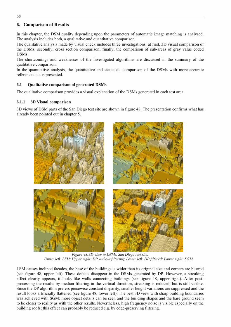
68

6. Comparison of Results

In this chapter, the DSM quality depending upon the parameters of automatic image matching is analysed. The analysis includes both, a qualitative and quantitative comparison. The qualitative analysis made by visual check includes three investigations: at first, 3D visual comparison of the DSMs; secondly, cross section comparison; finally, the comparison of sub-areas of gray value coded DSMs. The shortcomings and weaknesses of the investigated algorithms are discussed in the summary of the qualitative comparison. In the quantitative analysis, the quantitative and statistical comparison of the DSMs with more accurate reference data is presented.

6.1 Qualitative comparison of generated DSMs

The qualitative comparison provides a visual explanation of the DSMs generated in each test area.

6.1.1 3D Visual comparison

3D views of DSM parts of the San Diego test site are shown in figure 48. The presentation confirms what has already been pointed out in chapter 5.

Figure 48:3D-view to DSMs, San Diego test site;

Upper left: LSM; Upper right: DP without filtering; Lower left: DP filtered; Lower right: SGM

LSM causes inclined facades, the base of the buildings is wider than its original size and corners are blurred (see figure 48, upper left). These defects disappear in the DSMs generated by DP. However, a streaking effect clearly appears, it looks like walls connecting buildings (see figure 48, upper right). After post-processing the results by median filtering in the vertical direction, streaking is reduced, but is still visible. Since the DP algorithm prefers piecewise constant disparity, smaller height variations are suppressed and the result looks artificially flattened (see figure 48, lower left). The best 3D view with sharp building boundaries was achieved with SGM: more object details can be seen and the building shapes and the bare ground seem to be closer to reality as with the other results. Nevertheless, high frequency noise is visible especially on the building roofs; this effect can probably be reduced e.g. by edge-preserving filtering.

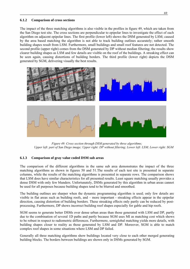
69

6.1.2 Comparison of cross sections

The impact of the three matching algorithms is also visible in the profiles in figure 49, which are taken from the San Diego test site. The cross sections are perpendicular to epipolar lines to investigate the effect of each algorithm on adjacent epipolar lines. The first profile (lower left) shows the DSM generated by LSM; caused by the area based matching the algorithm is not able to track building outlines accurately; rather smooth building shapes result from LSM. Furthermore, small buildings and small roof features are not detected. The second profile (upper right) comes from the DSM generated by DP without median filtering; the results show clearer building shapes as LSM and few details are visible on the roof of the buildings. A streaking effect can be seen again, causing distortions of building borders. The third profile (lower right) depicts the DSM generated by SGM, delivering visually the best results.

Figure 49: Cross section through DSM generated by three algorithms; Upper left: part of San Diego image; Upper right: DP without filtering; Lower left: LSM; Lower right: SGM

6.1.3 Comparison of gray value coded DSM sub areas

The comparison of the different algorithms in the same sub area demonstrates the impact of the three matching algorithms as shown in figures 50 and 51.The results of each test site is presented in separate columns, while the results of the matching algorithms is presented in separate rows. The comparison shows that LSM does have similar characteristics for all presented results. Least square matching usually provides a dense DSM with only few blunders. Unfortunately, DSMs generated by this algorithm in urban areas cannot be used for all purposes because building shapes tend to be blurred and smoothed.

The building outlines are sharper when the dynamic programming algorithm is used; only few details are visible in flat areas such as building roofs, and – more important - streaking effects appear in the epipolar direction, causing distortion of building borders. These streaking effects only partly can be reduced by post-processing. Furthermore, DP shows incorrect building roof shapes especially for gable and hip roofs.

SGM seems to generate better DSMs over dense urban areas than those generated with LSM and DP, partly due to the combination of several 1D paths and partly because SGM uses MI as matching cost which shows to be robust in respect to radiometric differences. Furthermore, semiglobal matching yields more details, with building shapes closer to reality as those generated by LSM and DP. Moreover, SGM is able to match complex roof shapes in some situations where LSM and DP failed.

Generally all three matching algorithms show buildings located very close to each other merged generating building blocks. The borders between buildings are shown only in DSMs generated by SGM.

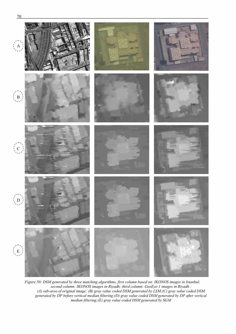
70

A

B

C

D

E

Figure 50: DSM generated by three matching algorithms, first column based on: IKONOS images in Istanbul;

second column: IKONOS images in Riyadh; third column: GeoEye-1 images in Riyadh ; (A) sub-area of original image; (B) gray value coded DSM generated by LSM;(C) gray value coded DSM

generated by DP before vertical median filtering;(D) gray value coded DSM generated by DP after vertical median filtering;(E) gray value coded DSM generated by SGM

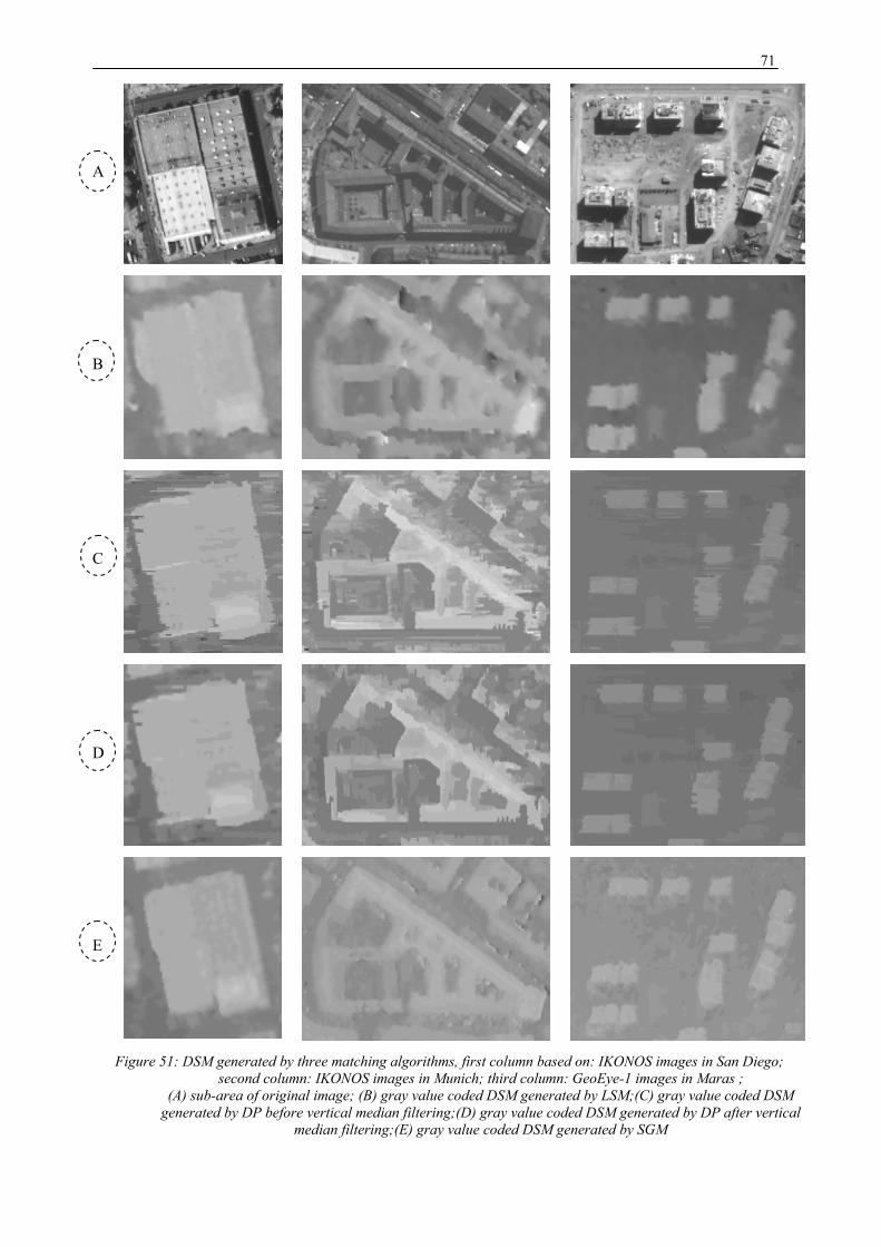
71

A

B

C

D

E

Figure 51: DSM generated by three matching algorithms, first column based on: IKONOS images in San Diego;

second column: IKONOS images in Munich; third column: GeoEye-1 images in Maras ; (A) sub-area of original image; (B) gray value coded DSM generated by LSM;(C) gray value coded DSM

generated by DP before vertical median filtering;(D) gray value coded DSM generated by DP after vertical median filtering;(E) gray value coded DSM generated by SGM

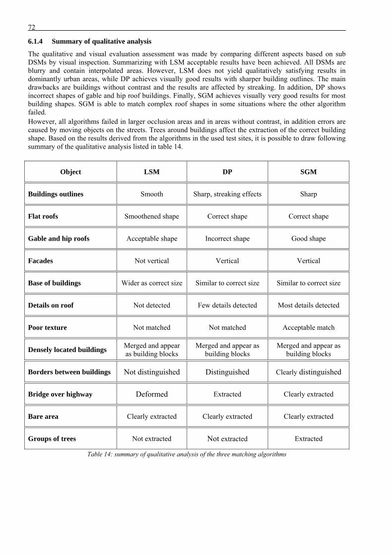
72

6.1.4 Summary of qualitative analysis

The qualitative and visual evaluation assessment was made by comparing different aspects based on sub DSMs by visual inspection. Summarizing with LSM acceptable results have been achieved. All DSMs are blurry and contain interpolated areas. However, LSM does not yield qualitatively satisfying results in dominantly urban areas, while DP achieves visually good results with sharper building outlines. The main drawbacks are buildings without contrast and the results are affected by streaking. In addition, DP shows incorrect shapes of gable and hip roof buildings. Finally, SGM achieves visually very good results for most building shapes. SGM is able to match complex roof shapes in some situations where the other algorithm failed. However, all algorithms failed in larger occlusion areas and in areas without contrast, in addition errors are caused by moving objects on the streets. Trees around buildings affect the extraction of the correct building shape. Based on the results derived from the algorithms in the used test sites, it is possible to draw following summary of the qualitative analysis listed in table 14.

Object LSM DP SGM

Buildings outlines Smooth Sharp, streaking effects Sharp

Flat roofs Smoothened shape Correct shape Correct shape

Gable and hip roofs Acceptable shape Incorrect shape Good shape

Facades Not vertical Vertical Vertical

Base of buildings Wider as correct size Similar to correct size Similar to correct size

Details on roof Not detected Few details detected Most details detected

Poor texture Not matched Not matched Acceptable match

Densely located buildings Merged and appear as building blocks

Merged and appear as building blocks

Merged and appear as building blocks

Borders between buildings Not distinguished Distinguished Clearly distinguished

Bridge over highway Deformed Extracted Clearly extracted

Bare area Clearly extracted Clearly extracted Clearly extracted

Groups of trees Not extracted Not extracted Extracted

Table 14: summary of qualitative analysis of the three matching algorithms

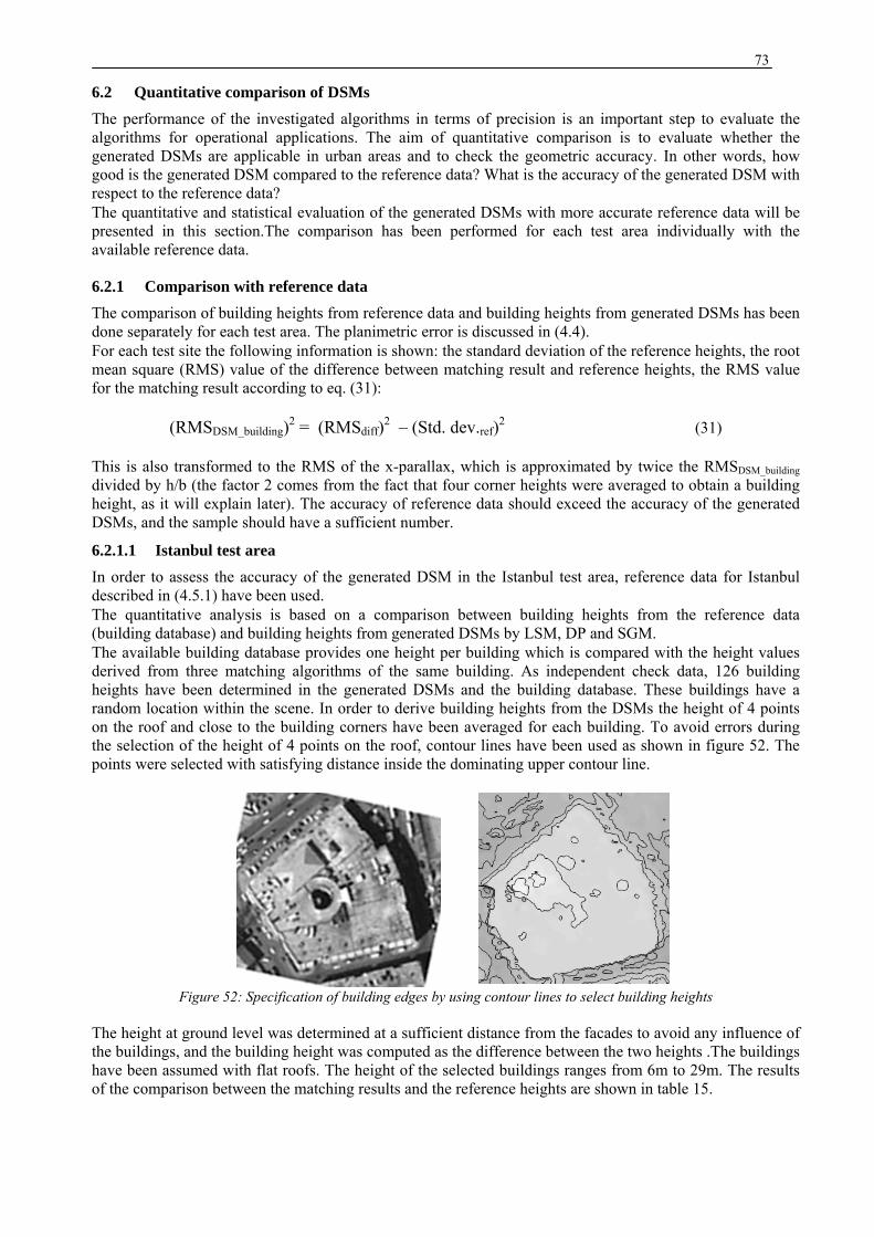
73

6.2 Quantitative comparison of DSMs The performance of the investigated algorithms in terms of precision is an important step to evaluate the algorithms for operational applications. The aim of quantitative comparison is to evaluate whether the generated DSMs are applicable in urban areas and to check the geometric accuracy. In other words, how good is the generated DSM compared to the reference data? What is the accuracy of the generated DSM with respect to the reference data? The quantitative and statistical evaluation of the generated DSMs with more accurate reference data will be presented in this section.The comparison has been performed for each test area individually with the available reference data.

6.2.1 Comparison with reference data The comparison of building heights from reference data and building heights from generated DSMs has been done separately for each test area. The planimetric error is discussed in (4.4). For each test site the following information is shown: the standard deviation of the reference heights, the root mean square (RMS) value of the difference between matching result and reference heights, the RMS value for the matching result according to eq. (31):

(RMSDSM_building)2 = (RMSdiff)2 – (Std. dev.ref)2 (31)

This is also transformed to the RMS of the x-parallax, which is approximated by twice the RMSDSM_building divided by h/b (the factor 2 comes from the fact that four corner heights were averaged to obtain a building height, as it will explain later). The accuracy of reference data should exceed the accuracy of the generated DSMs, and the sample should have a sufficient number.

6.2.1.1 Istanbul test area In order to assess the accuracy of the generated DSM in the Istanbul test area, reference data for Istanbul described in ( 4.5.1) have been used. The quantitative analysis is based on a comparison between building heights from the reference data (building database) and building heights from generated DSMs by LSM, DP and SGM. The available building database provides one height per building which is compared with the height values derived from three matching algorithms of the same building. As independent check data, 126 building heights have been determined in the generated DSMs and the building database. These buildings have a random location within the scene. In order to derive building heights from the DSMs the height of 4 points on the roof and close to the building corners have been averaged for each building. To avoid errors during the selection of the height of 4 points on the roof, contour lines have been used as shown in figure 52. The points were selected with satisfying distance inside the dominating upper contour line.

Figure 52: Specification of building edges by using contour lines to select building heights

The height at ground level was determined at a sufficient distance from the facades to avoid any influence of the buildings, and the building height was computed as the difference between the two heights .The buildings have been assumed with flat roofs. The height of the selected buildings ranges from 6m to 29m. The results of the comparison between the matching results and the reference heights are shown in table 15.

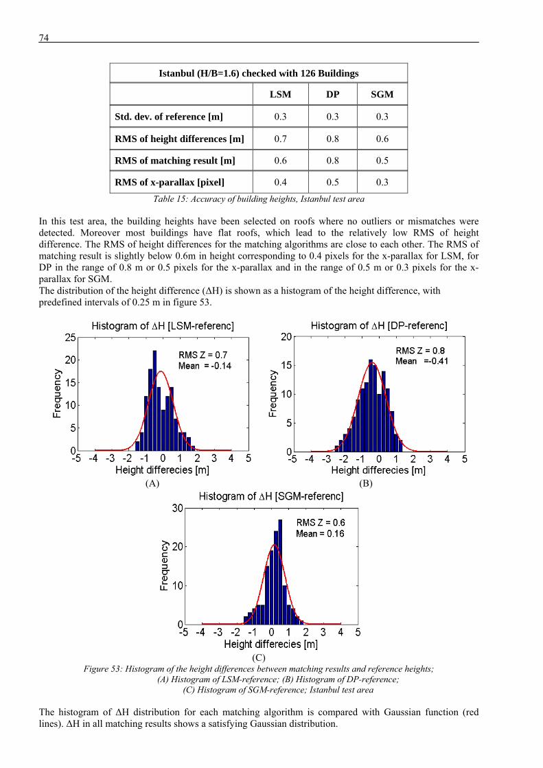
74

Istanbul (H/B=1.6) checked with 126 Buildings

LSM DP SGM

Std. dev. of reference [m] 0.3 0.3 0.3

RMS of height differences [m] 0.7 0.8 0.6

RMS of matching result [m] 0.6 0.8 0.5

RMS of x-parallax [pixel] 0.4 0.5 0.3 Table 15: Accuracy of building heights, Istanbul test area

In this test area, the building heights have been selected on roofs where no outliers or mismatches were detected. Moreover most buildings have flat roofs, which lead to the relatively low RMS of height difference. The RMS of height differences for the matching algorithms are close to each other. The RMS of matching result is slightly below 0.6m in height corresponding to 0.4 pixels for the x-parallax for LSM, for DP in the range of 0.8 m or 0.5 pixels for the x-parallax and in the range of 0.5 m or 0.3 pixels for the x-parallax for SGM. The distribution of the height difference (ΔH) is shown as a histogram of the height difference, with predefined intervals of 0.25 m in figure 53.

(A) (B)

(C) Figure 53: Histogram of the height differences between matching results and reference heights;

(A) Histogram of LSM-reference; (B) Histogram of DP-reference; (C) Histogram of SGM-reference; Istanbul test area

The histogram of ΔH distribution for each matching algorithm is compared with Gaussian function (red lines). ΔH in all matching results shows a satisfying Gaussian distribution.

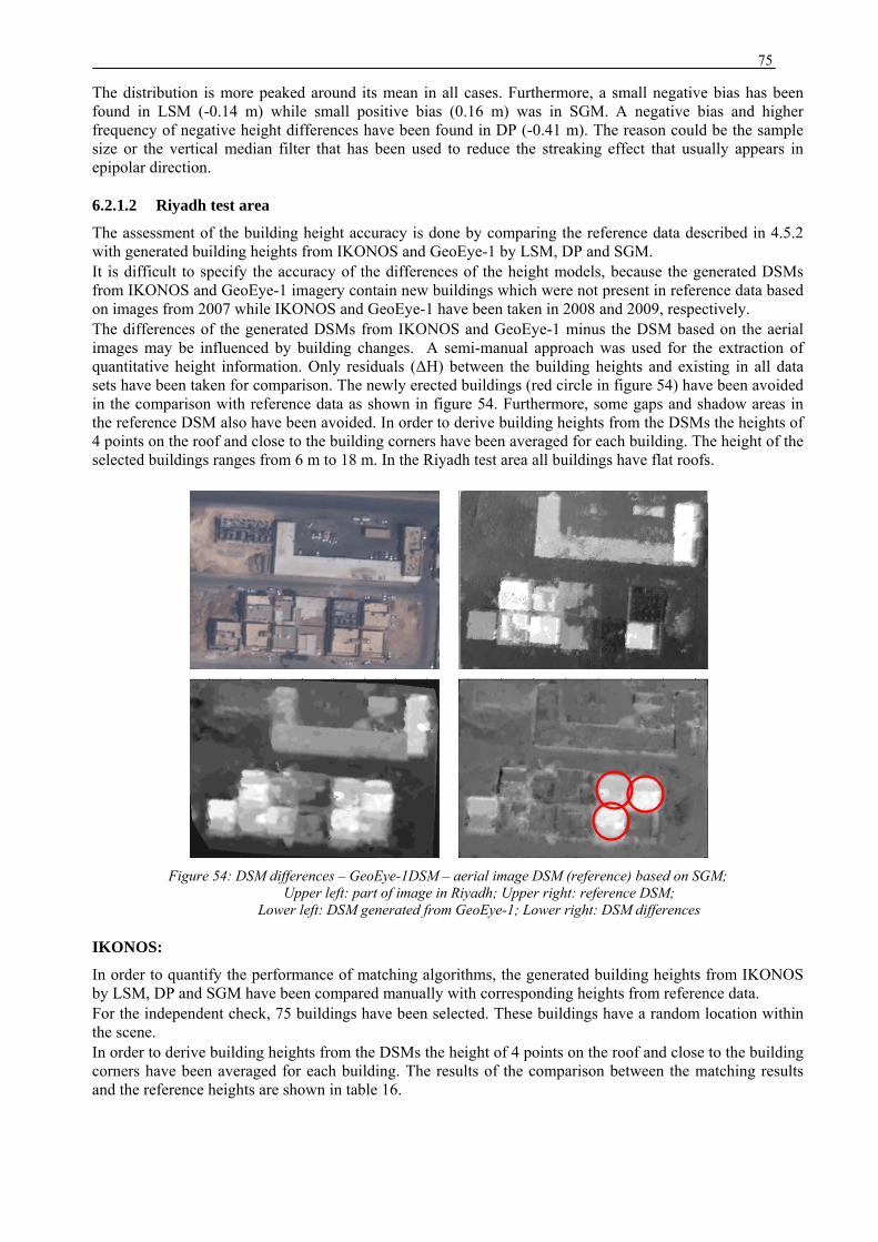
75

The distribution is more peaked around its mean in all cases. Furthermore, a small negative bias has been found in LSM (-0.14 m) while small positive bias (0.16 m) was in SGM. A negative bias and higher frequency of negative height differences have been found in DP (-0.41 m). The reason could be the sample size or the vertical median filter that has been used to reduce the streaking effect that usually appears in epipolar direction.

6.2.1.2 Riyadh test area

The assessment of the building height accuracy is done by comparing the reference data described in 4.5.2 with generated building heights from IKONOS and GeoEye-1 by LSM, DP and SGM. It is difficult to specify the accuracy of the differences of the height models, because the generated DSMs from IKONOS and GeoEye-1 imagery contain new buildings which were not present in reference data based on images from 2007 while IKONOS and GeoEye-1 have been taken in 2008 and 2009, respectively. The differences of the generated DSMs from IKONOS and GeoEye-1 minus the DSM based on the aerial images may be influenced by building changes. A semi-manual approach was used for the extraction of quantitative height information. Only residuals (ΔH) between the building heights and existing in all data sets have been taken for comparison. The newly erected buildings (red circle in figure 54) have been avoided in the comparison with reference data as shown in figure 54. Furthermore, some gaps and shadow areas in the reference DSM also have been avoided. In order to derive building heights from the DSMs the heights of 4 points on the roof and close to the building corners have been averaged for each building. The height of the selected buildings ranges from 6 m to 18 m. In the Riyadh test area all buildings have flat roofs.

Figure 54: DSM differences – GeoEye-1DSM – aerial image DSM (reference) based on SGM;

Upper left: part of image in Riyadh; Upper right: reference DSM; Lower left: DSM generated from GeoEye-1; Lower right: DSM differences

IKONOS:

In order to quantify the performance of matching algorithms, the generated building heights from IKONOS by LSM, DP and SGM have been compared manually with corresponding heights from reference data. For the independent check, 75 buildings have been selected. These buildings have a random location within the scene. In order to derive building heights from the DSMs the height of 4 points on the roof and close to the building corners have been averaged for each building. The results of the comparison between the matching results and the reference heights are shown in table 16.

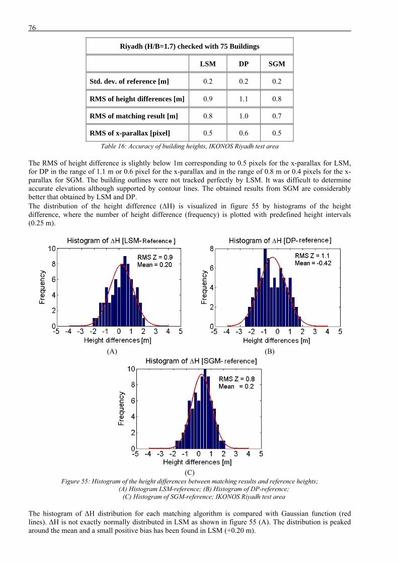
76

Riyadh (H/B=1.7) checked with 75 Buildings

LSM DP SGM

Std. dev. of reference [m] 0.2 0.2 0.2

RMS of height differences [m] 0.9 1.1 0.8

RMS of matching result [m] 0.8 1.0 0.7

RMS of x-parallax [pixel] 0.5 0.6 0.5

Table 16: Accuracy of building heights, IKONOS Riyadh test area

The RMS of height difference is slightly below 1m corresponding to 0.5 pixels for the x-parallax for LSM, for DP in the range of 1.1 m or 0.6 pixel for the x-parallax and in the range of 0.8 m or 0.4 pixels for the x-parallax for SGM. The building outlines were not tracked perfectly by LSM. It was difficult to determine accurate elevations although supported by contour lines. The obtained results from SGM are considerably better that obtained by LSM and DP. The distribution of the height difference (ΔH) is visualized in figure 55 by histograms of the height difference, where the number of height difference (frequency) is plotted with predefined height intervals (0.25 m).

(A) (B)

(C) Figure 55: Histogram of the height differences between matching results and reference heights;

(A) Histogram LSM-reference; (B) Histogram of DP-reference; (C) Histogram of SGM-reference; IKONOS Riyadh test area

The histogram of ΔH distribution for each matching algorithm is compared with Gaussian function (red lines). ΔH is not exactly normally distributed in LSM as shown in figure 55 (A). The distribution is peaked around the mean and a small positive bias has been found in LSM (+0.20 m).

77

The distribution of the ΔH from DP is also not exactly normal as shown in figure 55 (B), where a negative bias (-0.41 m) and higher frequency of negative height differences have been found in DP. As before the reason could be the small size or the vertical median filter that has been used to reduce the streaking effect that usually appears in epipolar direction.The histogram of the ΔH between the generated heights from SGM and reference heights seems to be closer to the normal distribution as for LSM and DP figure 55 (C); although a small positive bias (0.20 m) bias has been found. GeoEye-1: DSM generated from GeoEye-1 imagery with 0.50 m GSD shows clearer building details as DSM generated from the IKONOS image. As independent check data, the heights of 125 buildings have been compared manually with corresponding heights from reference data. These buildings have a random distribution within the scene. In order to derive building heights from the DSMs the height of 4 points on the roof and close to the building corners have been averaged for each building. The results of the comparison between the matching results and the reference heights are shown in table 17.

Riyadh (H/B=1.5) checked with 125 Buildings

LSM DP SGM

Std. dev. of reference [m] 0.2 0.2 0.2

RMS of height differences [m] 0.7 0.6 0.5

RMS of matching result [m] 0.6 0.5 0.4

RMS of x-parallax [pixel] 0.5 0.4 0.3

Table 17: Accuracy of building heights, Geo Eye-1 Riyadh test area

The vertical accuracies of the generated DSMs from GeoEye-1 images by three matching algorithms are below 0.7 m corresponding to 0.4 pixels for the x-parallax for LSM, for DP in the range of 0.6m or 0.4 pixels for the x-parallax and in the range of 0.5 m or 0.3 pixels for the x-parallax for SGM. Better results have been obtained by SGM. The histogram of ΔH for each matching algorithm is compared in figure 56 with Gaussian histograms (red lines). Figure 56 (A) shows a satisfying normal distribution of the results. LSM has a small bias of +0.07 m. ΔH errors are distributed on both sides of the mean. The histogram of ΔH from DP has a sharp peak at Mean (-0.48 m) as shown in figure 56 (B), where a negative bias (-0.48 m) and higher frequency of negative height differences have been found in DP. As before the reason could be also the small size or the vertical median filter that has been used to reduce the streaking effect that usually appears in epipolar direction. Ideally, the histogram of ΔH from SGM has a sharp peak at the difference zero. It seems closer to the normal distribution as LSM and DP, as shown in figure 56 (C), with a negligible positive bias of 0.06 m. There are no significant differences between the results from the three matching algorithms. These results let us assume that the results can be considered as representative for urban areas.

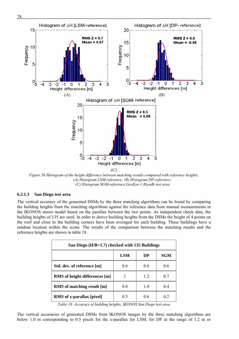
78

(A) (B)

(C) Figure 56:Histogram of the height difference between matching results compared with reference heights;

(A) Histogram LSM-reference; (B) Histogram DP-reference; (C) Histogram SGM-reference;GeoEye-1 Riyadh test area

6.2.1.3 San Diego test area

The vertical accuracy of the generated DSMs by the three matching algorithms can be found by comparing the building heights from the matching algorithms against the reference data from manual measurements in the IKONOS stereo model based on the parallax between the two points. As independent check data, the building heights of 135 are used. In order to derive building heights from the DSMs the height of 4 points on the roof and close to the building corners have been averaged for each building. These buildings have a random location within the scene. The results of the comparison between the matching results and the reference heights are shown in table 18.

San Diego (H/B=1.7) checked with 135 Buildings

LSM DP SGM

Std. dev. of reference [m] 0.6 0.6 0.6

RMS of height differences [m] 1 1.2 0.7

RMS of matching result [m] 0.8 1.0 0.4

RMS of x-parallax [pixel] 0.5 0.6 0.2

Table 18: Accuracy of building heights, IKONOS San Diego test area

The vertical accuracies of generated DSMs from IKONOS images by the three matching algorithms are below 1.0 m corresponding to 0.5 pixels for the x-parallax for LSM, for DP in the range of 1.2 m or

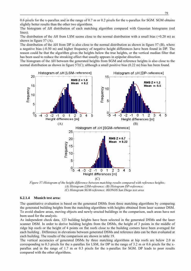
79

0.6 pixels for the x-parallax and in the range of 0.7 m or 0.2 pixels for the x-parallax for SGM. SGM obtains slightly better results than the other two algorithms. The histogram of ΔH distribution of each matching algorithm compared with Gaussian histograms (red lines). The distribution of the ΔH from LSM seems close to the normal distribution with a small bias (+0.20 m) as shown in figure 57 (A). The distribution of the ΔH from DP is also close to the normal distribution as shown in figure 57 (B), where a negative bias (-0.50 m) and higher frequency of negative height differences have been found in DP. The reason could be that the algorithm gives the heights below the true heights, or the vertical median filter that has been used to reduce the streaking effect that usually appears in epipolar direction. The histogram of the ΔH between the generated heights from SGM and reference heights is also close to the normal distribution as shown in figure 57(C); although a small positive bias (0.22 m) bias has been found.

(A) (B)

(C) Figure 57:Histogram of the height difference between matching results compared with reference heights;

(A) Histogram LSM-reference; (B) Histogram DP-reference; (C) Histogram SGM-reference; IKONOS San Diego test area

6.2.1.4 Munich test area: The quantitative evaluation is based on the generated DSMs from three matching algorithms by comparing the generated building heights from the matching algorithms with heights obtained from laser scanner DSM. To avoid shadow areas, moving objects and newly-erected buildings in the comparison, such areas have not been used for the analysis. As independent check data, 123 building heights have been selected in the generated DSMs and the laser scanner DSM. In order to derive building heights from the DSMs, the height of 3 points in the middle of ridge hip roofs or the height of 4 points on flat roofs close to the building corners have been averaged for each building . Difference in elevations between generated DSMs and reference data can be then evaluated at each building. The results of the comparison are shown in table 19. The vertical accuracies of generated DSMs by three matching algorithms at hip roofs are below 2.0 m corresponding to 0.3 pixels for the x-parallax for LSM, for DP in the range of 3.2 m or 0.6 pixels for the x-parallax and in the range of 1.7 m or 0.3 pixels for the x-parallax for SGM. DP leads to poor results compared with the other algorithms.

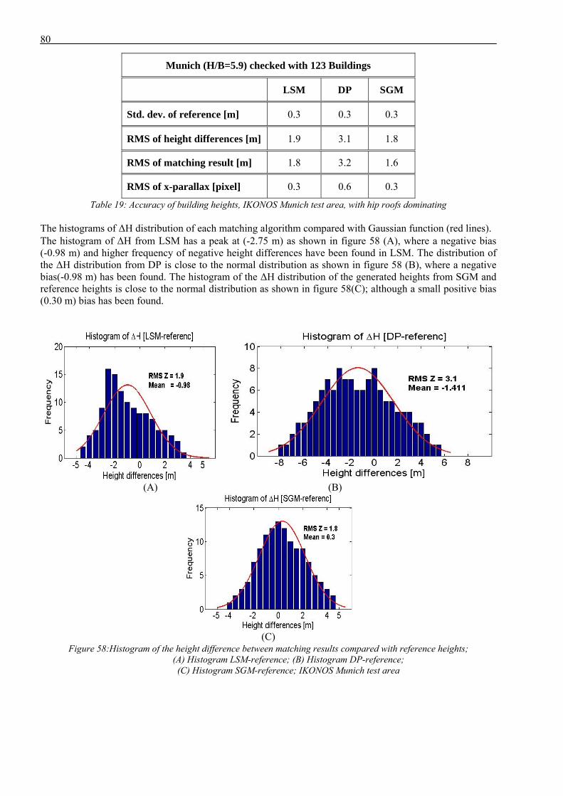
80

Munich (H/B=5.9) checked with 123 Buildings

LSM DP SGM

Std. dev. of reference [m] 0.3 0.3 0.3

RMS of height differences [m] 1.9 3.1 1.8

RMS of matching result [m] 1.8 3.2 1.6

RMS of x-parallax [pixel] 0.3 0.6 0.3

Table 19: Accuracy of building heights, IKONOS Munich test area, with hip roofs dominating

The histograms of ΔH distribution of each matching algorithm compared with Gaussian function (red lines). The histogram of ΔH from LSM has a peak at (-2.75 m) as shown in figure 58 (A), where a negative bias (-0.98 m) and higher frequency of negative height differences have been found in LSM. The distribution of the ΔH distribution from DP is close to the normal distribution as shown in figure 58 (B), where a negative bias(-0.98 m) has been found. The histogram of the ΔH distribution of the generated heights from SGM and reference heights is close to the normal distribution as shown in figure 58(C); although a small positive bias (0.30 m) bias has been found.

(A) (B)

(C) Figure 58:Histogram of the height difference between matching results compared with reference heights;

(A) Histogram LSM-reference; (B) Histogram DP-reference; (C) Histogram SGM-reference; IKONOS Munich test area

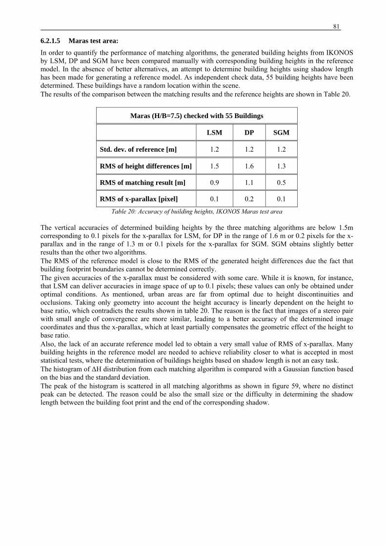
81

6.2.1.5 Maras test area:

In order to quantify the performance of matching algorithms, the generated building heights from IKONOS by LSM, DP and SGM have been compared manually with corresponding building heights in the reference model. In the absence of better alternatives, an attempt to determine building heights using shadow length has been made for generating a reference model. As independent check data, 55 building heights have been determined. These buildings have a random location within the scene. The results of the comparison between the matching results and the reference heights are shown in Table 20.

Maras (H/B=7.5) checked with 55 Buildings

LSM DP SGM

Std. dev. of reference [m] 1.2 1.2 1.2

RMS of height differences [m] 1.5 1.6 1.3

RMS of matching result [m] 0.9 1.1 0.5

RMS of x-parallax [pixel] 0.1 0.2 0.1

Table 20: Accuracy of building heights, IKONOS Maras test area

The vertical accuracies of determined building heights by the three matching algorithms are below 1.5m corresponding to 0.1 pixels for the x-parallax for LSM, for DP in the range of 1.6 m or 0.2 pixels for the x-parallax and in the range of 1.3 m or 0.1 pixels for the x-parallax for SGM. SGM obtains slightly better results than the other two algorithms. The RMS of the reference model is close to the RMS of the generated height differences due the fact that building footprint boundaries cannot be determined correctly. The given accuracies of the x-parallax must be considered with some care. While it is known, for instance, that LSM can deliver accuracies in image space of up to 0.1 pixels; these values can only be obtained under optimal conditions. As mentioned, urban areas are far from optimal due to height discontinuities and occlusions. Taking only geometry into account the height accuracy is linearly dependent on the height to base ratio, which contradicts the results shown in table 20. The reason is the fact that images of a stereo pair with small angle of convergence are more similar, leading to a better accuracy of the determined image coordinates and thus the x-parallax, which at least partially compensates the geometric effect of the height to base ratio. Also, the lack of an accurate reference model led to obtain a very small value of RMS of x-parallax. Many building heights in the reference model are needed to achieve reliability closer to what is accepted in most statistical tests, where the determination of buildings heights based on shadow length is not an easy task. The histogram of ΔH distribution from each matching algorithm is compared with a Gaussian function based on the bias and the standard deviation. The peak of the histogram is scattered in all matching algorithms as shown in figure 59, where no distinct peak can be detected. The reason could be also the small size or the difficulty in determining the shadow length between the building foot print and the end of the corresponding shadow.

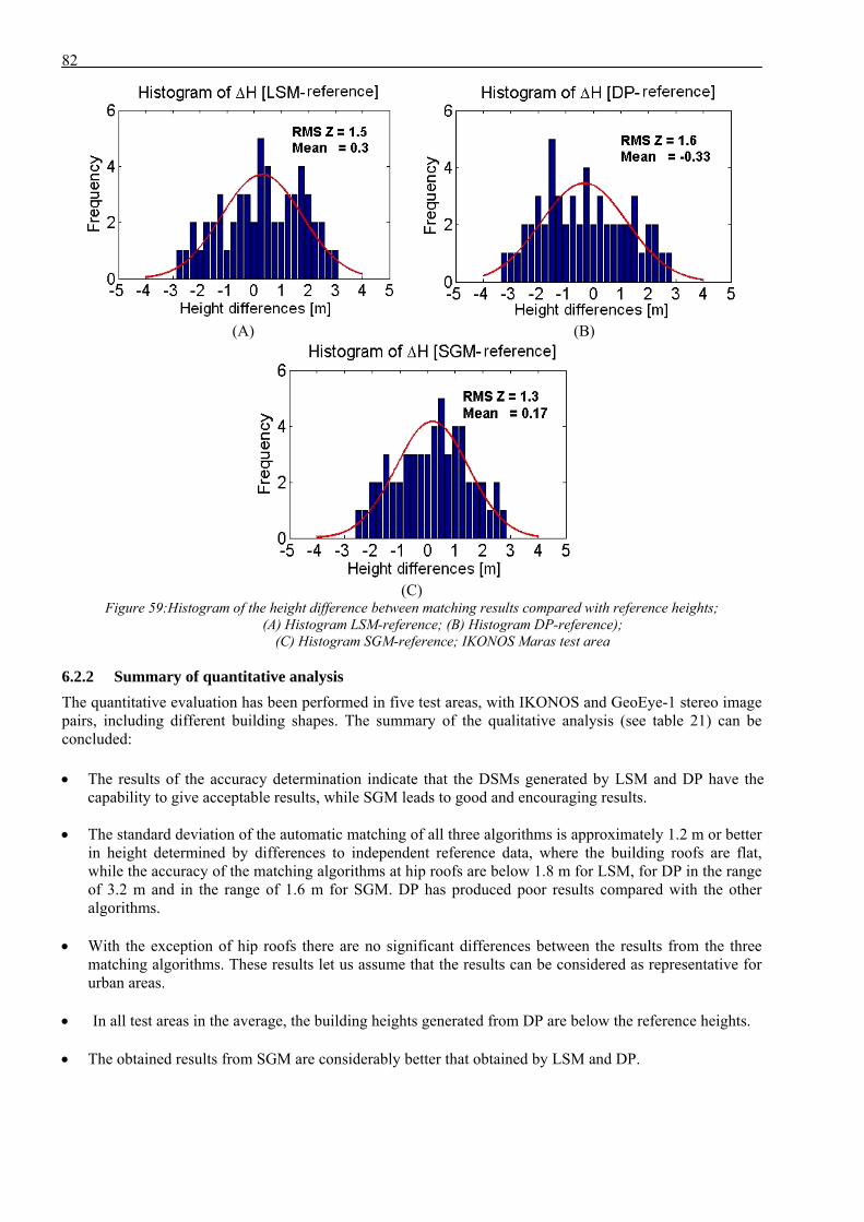
82

(A) (B)

(C) Figure 59:Histogram of the height difference between matching results compared with reference heights;

(A) Histogram LSM-reference; (B) Histogram DP-reference); (C) Histogram SGM-reference; IKONOS Maras test area

6.2.2 Summary of quantitative analysis The quantitative evaluation has been performed in five test areas, with IKONOS and GeoEye-1 stereo image pairs, including different building shapes. The summary of the qualitative analysis (see table 21) can be concluded:

• The results of the accuracy determination indicate that the DSMs generated by LSM and DP have the capability to give acceptable results, while SGM leads to good and encouraging results.

• The standard deviation of the automatic matching of all three algorithms is approximately 1.2 m or better in height determined by differences to independent reference data, where the building roofs are flat, while the accuracy of the matching algorithms at hip roofs are below 1.8 m for LSM, for DP in the range of 3.2 m and in the range of 1.6 m for SGM. DP has produced poor results compared with the other algorithms.

• With the exception of hip roofs there are no significant differences between the results from the three

matching algorithms. These results let us assume that the results can be considered as representative for urban areas.

• In all test areas in the average, the building heights generated from DP are below the reference heights. • The obtained results from SGM are considerably better that obtained by LSM and DP.

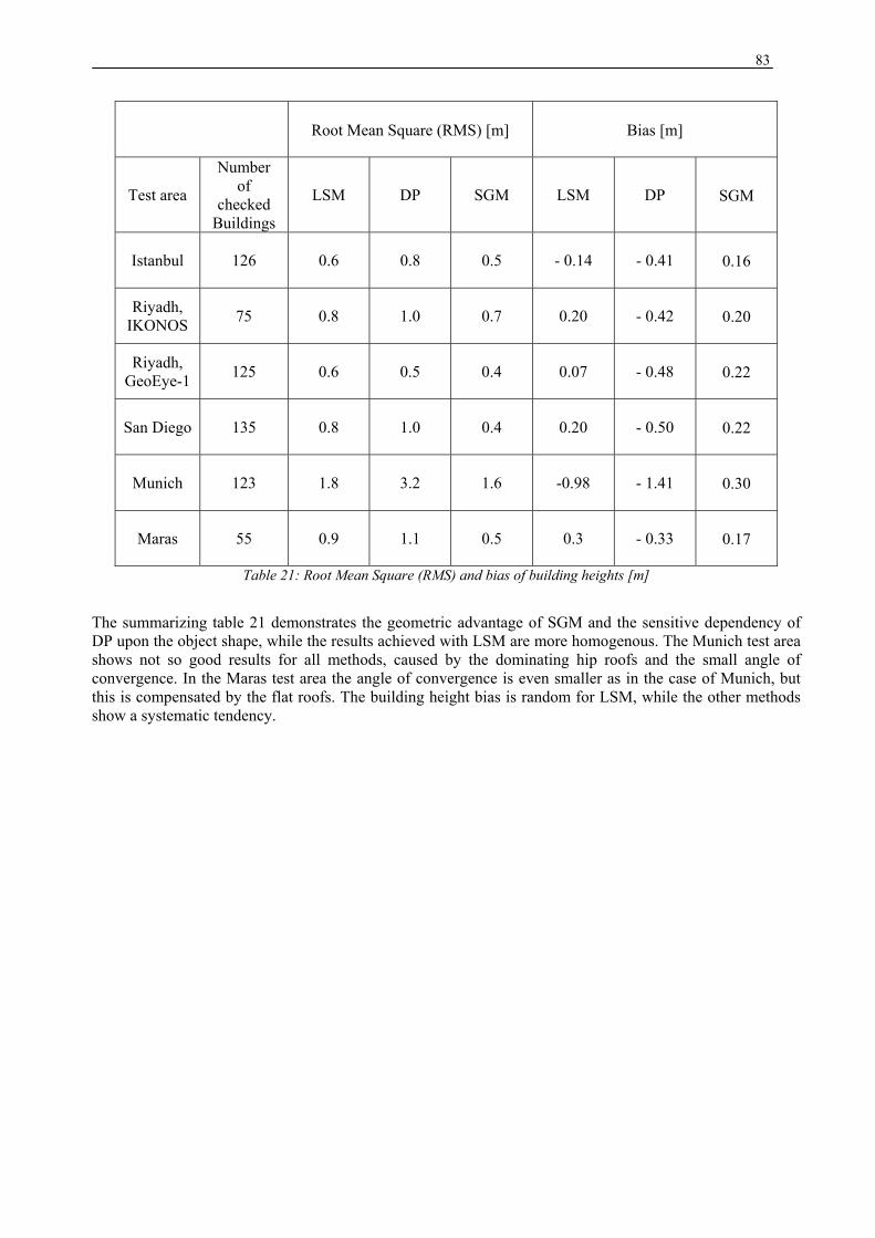
83

Root Mean Square (RMS) [m]

Bias [m]

Test area

Number of

checked Buildings

LSM DP SGM LSM DP

SGM

Istanbul 126 0.6 0.8 0.5 - 0.14 - 0.41

0.16

Riyadh, IKONOS 75 0.8 1.0 0.7 0.20 - 0.42

0.20

Riyadh, GeoEye-1 125 0.6 0.5 0.4 0.07 - 0.48

0.22

San Diego 135 0.8 1.0 0.4 0.20 - 0.50

0.22

Munich 123 1.8 3.2 1.6 -0.98 - 1.41

0.30

Maras 55 0.9 1.1 0.5 0.3 - 0.33

0.17

Table 21: Root Mean Square (RMS) and bias of building heights [m]

The summarizing table 21 demonstrates the geometric advantage of SGM and the sensitive dependency of DP upon the object shape, while the results achieved with LSM are more homogenous. The Munich test area shows not so good results for all methods, caused by the dominating hip roofs and the small angle of convergence. In the Maras test area the angle of convergence is even smaller as in the case of Munich, but this is compensated by the flat roofs. The building height bias is random for LSM, while the other methods show a systematic tendency.

84

7. Final Conclusions and Outlook

7.1 Conclusion

This investigation and development has covered a number of issues related to the generation of DSM from very high resolution satellite stereo image pairs in urban areas, particularly image orientation, epipolar image generation, and image matching. All these issues are implemented and tested, and it can be concluded that the research objectives have been reached. The aspects are summarized as follows: • The geometric accuracy has been determined by means of reference data; orientation accuracy in the

range of one pixel has been reached. • The generated epipolar pairs are examined by means of seed points and least squares matching for

remaining y-parallaxes. No significant y-parallaxes are detected, the remaining y-parallax was always well below one pixel.

• The control parameters of the three matching algorithms have been determined empirically based on visual inspection of the generated DSMs. The optimal fitting set of control parameters for each test areas finally was used.

• The quality of a generated DSM depends on the quality of very high resolution satellite stereo image pairs, the characteristics of the object and the matching method.

• The qualitative and visual evaluation of the digital surface models derived by the three matching algorithms has been conducted. The investigated algorithms show differences in detail and shape of objects:

(1) Least square matching with region growing provides a DSM with only few blunders. Due to the use of a fixed template size the street level, façade of building and roof top of the building are merged. At building facades LSM takes an average height between top of building and street level. So building outlines seem to be fuzzy and deformed into blobs. The base of the buildings is wider than its original size. Larger occlusions in the case of small height to base relation cause a loss of some matched points at building facades, which are not visible in both images. The algorithm failed in extracting details of small houses. Densely located buildings are merged and appear as building blocks where the hidden parts are not matched. Problems occur in occlusion areas, on homogenous roof tops and streets. Some errors in the generated DSM correspond to moving objects on the streets and low contrast areas.

(2) Dynamic programming requires epipolar images and as post-processing median filters across the epipolar lines to reduce streaking. DP achieves visually good results with sharper building outlines. DP shows incorrect shapes of gable and hip roofs due to optimization problem, where the optimization is carried out for corresponding epipolar line pairs separately. Buildings which are very close to each other are merged and appear as building blocks. The main reason for mismatching is caused by buildings without texture. However, if there is no accompanying intensity variation for several epipolar lines, boundaries of buildings cannot be detected. Errors are caused by moving objects on the streets. Trees around buildings affect the extraction of the correct building shape.

(3) Semiglobal matching requires epipolar images. It leads to improved DSMs compared to LSM and DP; no streaking can be seen. There are no large errors in the generated DSMs. Building outlines seem to be sharp as in the original image, but some inaccurate points appear especially at building edges due to shadows. Details on the roof of the building are clearly be extracted. Some unrealistic values appear at larger occlusions especially in case of larger convergence angles. Spaces between buildings appear clearly. Buildings located very close to each other are merged and appear as building blocks. SGM is able to generate a qualified DSM in dense urban areas even for buildings with gable and hip roofs where DP fails.

• The quantitative and statistical evaluation of the generated DSMs in relation to reference data has been performed. The comparison has been made for all test areas and all data sets. The standard deviation for the building height of the automatic matching of all three algorithms is approximately 1.2 m or better where the building roofs are flat, while the accuracy of the matching algorithms at hip roofs are below 1.8 m for LSM, for DP in the range of 3.2 m and in the range of 1.6 m for SGM.

In general it is possible to generate DSMs by automatic image matching in urban areas with a quality acceptable for a number of applications using very high resolution satellites images. Other applications requiring more details, completeness or faithfulness in building shape need higher resolution images and some degree of manual intervention.

85

7.2 Outlook This thesis can support the operational use of the described algorithms. During the investigation very good results were obtained with the investigated aalgorithms, but nevertheless there is a potential for further improvement. Future works will be focused on: • Outlier detection and automatic removal from generated DSMs. Some known techniques for detecting

and removing invalid matches in generated DSMs can be applied, including left-right and right-left consistency checks. This process can also be done with the disparity map before image orientation.

• In this thesis image matching has been processed by using only two overlapping images; this locally leads to unsatisfactory results due the occlusion which is a main source of mismatches. More images with different view angles would improve the accuracy and reliability.

• Local Wallis filtering (Pfluger, et al., 1987) for contrast enhancement can be applied to optimize the images for image matching. The effects of radiometric problems may be reduced especially in very dark image parts

• The used LSM may be improved by an adaptive window, where the algorithm is modifying the window size and shape adaptively according to the local intensity and disparity variations.

• The used LSM with region growing requires at least one seed point (start points for matching), provided by manual measurement in both images, an algorithm can be proposed to provide a set of seed points automatically. SIFT (Scale Invariant Feature Transform) (Lowe, 2004) may be a promising method for this purpose.

• To reduce the influence of noise in SGM, aggregation cost can be computed by summing the calculated matching costs over a small window (5×5 pixels) with constant disparity.

• A building monitoring may be supported by the shape analysis of differential DSMs able to separate between buildings and noise to use the results directly for map update.

• Buildings with some trees around, did not lead to a clear building shape. Therefore, trees can be identified by Normalised Difference Vegetation Index (NDVI) and height variation and respected in the DSM.

The automatic generation of digital surface models in urban areas based on IKONOS stereo pairs using image matching techniques has reached a high level of quality. The three investigated methods show differences in detail and object shape. In general it is possible to generate DSMs automatically in urban areas with a quality acceptable for a number of applications using very high resolution satellite images. Other applications requiring more object details, completeness or reliability in building shape, need higher resolution images and some degree of manual intervention. An operational method for the determination of clear building structures as base for a 3D city model has been developed and can be used for practical application.

86

8. Reference

Ackermann, F. (1984). Digital image correlation:performance and potential application in photogrammetry. photogrammetric Record ,Vol.11 (No.64), pp.429-439.

Allam, M. (1978). DTM's Application in Topographic mapping. Proc. of the DTM Symposium, pp.1-15, Louis.

Alobeid, A.; Jacobsen, K.; Heipke, C.;. (2010). Comparison of Matching Algorithms for DSM Generation in Urban Areas from Ikonos Imagery. Photogrammetric Engineering & Remote Sensing ,Vol.76(9),pp.1041-1050.

Anil, A., Nasser, K., & Mihai, N. (2007). Stereo matching via selective multiple windows. Journal of Electronic Imaging ,Vol.16(1)

Baillard, C.; Dissard, O.;. (2000). A stereo matching algorithm for urban digital elevation models. journal Photogrammetric Engineering & Remote Sensing ,Vol.66(9),pp.1119-1128.

Baltsavias, E.P.; Stallmann, D. (1992). From Satellite Images to GIS with Digital Photogrammetry Using SPOT Data. In Proc.of EGIS 92, Vol.2, pp. 945-946.

Benard, M.; Boutaleb, A.-K.; Kölbl, O.; Penis, C.;. (1986). Automatic stereophotogrammetry:implementation and comparison of classical correlation methods and dynamic programming based techniques. International Archives of Photogrammetry, Remote Sensing and Spatial Information Sciences, Vol.26 (3/3), pp. 131-140.

Birchfield, S.; Tomasi, C.;. (1998). A pixel dissimilarity measure that is insensitive to image sampling. IEEE Transactions on Pattern Analysis and Machine Intelligence, 20(4), pp.401-406.

Birchfield, S.; Tomasi, C.;. (1999). Depth discontinuities by pixel-to-pixel stereo. International Journal of Computer Vision ,Vol.35(3), pp.269-293.

Bobick, A.F.; Intille, S.;. (1999). Large occlusion stereo. International Journal on Computer Vision (IJCV), Vol.33/3),pp. 181-200.

Boykov, Y.; Veksler, O.; Zabih, R. (1998). A variable window approach to early vision. IEEE PAMI, Vol.20(12), pp. 1283-1294.

Boykov, Y.; Veksler, O.; Zabih, R. (1999). Fast approximate energy minimization via graph cuts. International Conference on Computer Vision, Vol.1, pp. 377-384.

Brito, J.L.N.S.; Silveira, M.T.; Jacobsen, K.; Amorim, S.; Mota, G.L.A.; Feitosa, R.Q.; Heipke, C.;. (2008). Monitoring of Height Changes in Urban Area from Multi-Platform Remotely sensed Data. The International Archives of the Photogrammetry, Remote Sensing and Spatial Information Sciences, vol.37(B1), pp. 835-840. Beijing.

Brown, M.Z.; Burschka, D.; Hager, G.D.;. (2003). Advances in computational stereo. IEEE Transactions on Pattern Analysis and Machine Intelligence ,Vol.25(8),pp. 993-1008.

Büyüksalih, G.; Jacobsen, K.;. (2007). Digital Surface Models in Build up Areas based on very high resolution Space Images. Proceedings of the ASPRS 2007 Annual conference 7-11 May, Tampa (pp. unpaginated CD-ROM). also available at www.ipi.uni-hannover.de (last access April 2011).

Caetano, M.; Santos, T. (2001). Updating land cover maps with satellite images. Geoscience and Remote Sensing Symposium, IGARSS '01. IEEE, Vol.3, pp. 979-981.

Canny, J.;. (1986). A computational approach to edge detection. IEEE Transactions on Pattern Analysis and Machine Intelligence, Vol.8(6), pp. 679-698.

Chan, S.; Wong, Y.; Daniel, J.;. (2003). Dense stereo correspondence based on recursive adaptive size multi-windowing. Image and Vision , Vol.1, pp. 256-260. New Zealand recursive adaptive size multi-windowing.

Chehata, N.; Jung, F.; Stamon, G.;. (2009). A graph cut optimization guided by 3D-features for surface height recover. ISPRS Journal of Photogrammetry and Remote Sensing , Vol.64, pp.193-203.

Chehata, N.; Pierrot - Desseilligny, M.; Jung, F.; Stamon, G.;. (2002). Extraction of 3d primitives from stereopairs of satellite images for automatic reconstruction of buildings. IAPR Workshop on Machine Vision Applications, pp. 636-640,Nara, Japan.

87

Chehata, N.; Pierrot-Deseilligny, M.; Stamon, G.;. (2005). Hybrid DEM generation constrained by 3D-primitives : A global optimization algorithm using graph cuts. IEEE International Conference on Image Processing ICIP'05, pp. 117-120, Genoa, Italia.

Chen, A.J.; Liu, C.H.; Rau, J.Y.; Chen, L.C.;. (1994). Adaptive Stereo Matching for SPOT Multispectral Image Pairs. SPIE Proceedings, Vol.30(3), pp. 98-103.

Christoudias, C.; Georgescu, B.; Meer, P.;. (2002). Synergism in Low Level Vision. 16th International Conference on Pattern Recognition, Vol.4, pp. 150-155. Quebec City, Canada.

Cox, I..; Hingorani, S.; M.Maggs, B.; B.Rao., B.;. (1992). Stereo without disparity gradient smoothing:a Bayesian sensor fusion solution. British Machine Vision Conference, pp. 337-347, Leeds, UK.

Cox, I., Hingorani, S., Maggs, B. M., & Rao., S. B. (1996). A maximum likelihood stereo algorithm. Computer Vision and Image Understanding , Vol.63(3), 542-567.

David, L.,. (2004). Distinctive Image Features from Scale Invariant key points. International Journal of Computer Vision , pp.91-110.

Di, Kaichang; Ma, Ruijin; Li, Rongxing;. (2003). Geometric Processing of Ikonos Stereo Imagery for Coastal Mapping Applications. Photogrammetric engineering & Remote Sensing , Vol.69,No.8, pp.873-879.

Doyle, F. (1978). Digital Terrain Models: An Overview. Photogrammetric Engineering & Remote Sensing , Vol.44, pp.1481-1487.

Dursun, S.; Sagir, D.; Büyüksalih, G.; Buhur, S.;. (2008). 3D City Modelling of Istanbul Historic Peninsula by Combination of Aerial Images and Terrestrial Laser Scanning Data. 28th EARSeL Annual Symposium, (pp. unpaginated CD-ROM).

Egnal, G. (2000). Mutual information as a stereo correspondence measure.Technical Report MS-CIS-00-20: University of Pennsylvania

Falkner, E. (1995). Aerial Mapping, Methods and Applications. 1st Ed. London, pp. 1-7, Lewis Publisgers.

Flamanc, D.; Maillet, G.;. (2005). Evaluation of 3D city model production from Pleiades-HR satellite images and 2D ground maps. International Archives of Photogrammetry, Remote Sensing and Spatial Information Sciences, Vol.36(8/w27). Tempe,AZ,USA.

Forney, G. D. (1973). The Viterbi Algorithm. Proceeding of the IEEE ,Vol.61(3), pp.268-278.

Förstener, W.; Gülch, E.;. (1987). A fast operator for detection and precise location of distinct points, corners and centers of circular features. Proceedings of ISPRS Intercommission Conference on Fast Processing of Photogrammetric Data, pp. 281-305,Interlaken, Switzerland.

Förstner, W. (1982). On the geometric precision of digital correlation. IAPRS , Vol.26 (No.3/3), 176-189.

Fraser, C.S.; Baltsavias, E.; Gruen, A. (2001). 3D building reconstruction from high-resolution Ikonos stereo imagery. In Automatic Extraction of Man-Made Objects from Aerial and Space Images.A A Balkema(Lisse).

Fraser, C.S.; Baltsavias, E.; Gruen, A.;. (2001). 3D building reconstruction from high-resolution Ikonos stereo-imagery. (A. a. Edited by E.P.Baltsavias, Ed.) Balkema, Tokyo: Automatic Extraction of Man-Made Objects From Aerial and Space Images (III).

Fusiello, A.; Roberto, V.; Trucco, E.;. (1997). Efficient stereo with multiple windowing. Conference on Computer Vision and Pattern Recognition, pp. 858-863, Puerto Rico.

Geiger, D., Ladendorf, B., & Yuille, A. (1995). Occlusions and binocular stereo. International Journal on Computer Vision ,Vol.14,pp.211-226.

Grodecki, J.;. (2001). Ikonos stereo feature extraction - RPC approach. American Society for Photogrammetry and Remote Sensing Conference, St. Louis ,p. p.7, on CD-ROM.

Grün, A.;. (1985). Adaptive Least Squares Correlation Correlation: A Powerful Image Matching Technique. South Africa Journal of Photogrammetry, Remote Sensing and Cartography , Vol. 14, No.3, 175-187.

Haala, N. (2009). Comeback of digital image matching. in Fritsch (ed.), Photogrammetric Week, pp. 289-301, Heidelberg.

Heipke, C. (1996). Overview of image matching techniques. 16th OEEPE Workshop on Application of Digital Photogrammetric Workstation. Lausanne.

88

Heipke, C.; Oberst, J.; Albertz, J.; Attwenger, M.; Dorninger, P.; Dorrer, E.; Ewe, M.; Gehrke, M.; Gwinner, K.; Hirschmüller, H.; Kim, J.R.; Kirk, R.L.; Mayer, H.; Muller, J.-P.; Rengarajan, R.; Rentsch, M.; Schmidt, R.; Scholten, F.; Shan, J.; Spiegel, M.; Wählisch, M.; Neukum, G.; HRSC Co-Investigator Team;. (2007). Evaluating planetary digital terrain models – the HRSC DTM test. Planetary and Space Science , Vol.(55) 14,pp. 2173-2191. Hirschmüller, H.; Innocent, P.; Garibaldi, J. (2002). Real-time correlation-based stereo vision with reduced border errors. Computer Vision , Vol.47, pp.229-246. Hirschmüller, H. (2006). Stereo Vision in Structured Environments by Consistent Semiglobal Matching. IEEE Conf. on Computer Vision and Pattern Recognition CVPR'06, Vol. 2, pp. 2386-2393. New York, NY, USA. Hirschmüller, H. (2008). Stereo Processing by Semiglobal Matching and Mutual Information. IEEE Transactions on Pattern Analysis and Machine Intelligence, Vol.30(2), pp. 328-341. Hirschmüller, H.; Scharstein, D. (2009). Evaluation of Stereo Matching Costs on Images with Radiometric Differences. IEEE Transactions on Pattern Analysis and Machine Intelligence , pp. 1582-1599. Ishikawa, H.; Geiger, D.;. (1998). Occlusions, discontinuities, and epipolar lines in stereo. 5th European Conference on Computer Vision, Vol.1, pp. unpaginated CD-ROM, Freiburg,Germany. Jacobsen, K. (2003). Geometric Potential of IKONOS and QuickBird-Images. In: Fritsch (Ed.):Photogrammetric Week '03, pp. 101-110,Wichmann Verlag, Heidelberg. Jacobsen, K.; Büyüksalih, G.; Topan, H. (2005). Geometric Models for the Orientation of High Resolution Optical Satellite Sensors. International Archives of Photogrammetry, Remote Sensing and Spatial Information Sciences. Hannover: 36 (1/w3), pp. unpaginated CD-ROM. Jacobsen, K.;. (2006). Digital surface models of city areas by very high resolution space imagery. Proceedings of the 1st workshop of the EARSeL-SIG Urban Remote Sensing (pp. unpaginated CD-ROM). available at www.ipi.uni-hannover.de (last accessed: April 2011). Kanade, T.; Okutomi, M.;. (1994). A stereo matching algorithm with an adaptive window. theory and experiment ,IEEE Transactions on Pattern Analysis and Machine Intelligence , Vol.16 (No.9), pp.920-932. Kim, J.; Kolmogorov., V.; Zabih, R.;. (2003). Visual correspondence using energy minimization and mutual information. IEEE International Conference Computer Vision, Vol.2, pp.1033-1040. Kim, T.; Im, Y-J.; Kim, H-W.; Kweon, I-S.;. (2002). DEM generation from an IKONOS Stereo Pair using EpiMatch and Graph Cut Algorithms. Proc. of International Symposium on Remote Sensing (18th Fall Symposium of KSRS), pp. 524-529. Sok-Cho. Konecny, G. (1998). Remote Sensing for Sustainable Development – State of the Art. EARSeL Advances. Krauß, T.; Lehner, M.; Reinartz, P.; Schroeder, M.; Stilla, U.;. (2005). DEM generation from very high resolution stereo satellite data in urban areas using dynamic programming. International Archives of Photogrammetry, Remote Sensing and Spatial Information Sciences, Vol.36 (1/W3), pp. unpaginated CD-ROM. Krauß, T.; Lehner, M.; Reinartz, P.;. (2007). Modeling of Urban Areas from High Resolustion stereo Satellite Images. International Archives of Photogrammetry, Remote Sensing and Spatial Information Sciences, Vol.36,Band 1/W51, pp. unpaginated CD-ROM. Hannover. Krauß, T.; Lehner, M.; Reinartz, P.;. (2008). Generation of coarse 3D models of urban areas from high resolution stereo satellite images. International Archives of Photogrammetry, Remote Sensing and Spatial Information Sciences, Vol.(37/B1), pp. 1091-1098. Kux, H.; Pinho, D.; Souza, I. (2006). High-Resolution Satellite Images for Urban Planning. International Archives of Photogrammetry,Remote Sensing and Spatial Information Sciences, vol.36(2), pp. 121-124. Lane, R.A.; Thacker, N.A.; Seed, N.L.;. (1994). Stretch-correlation as a realtime alternative to feature-based stereo matching algorithms. IVC , Vol.12 (4), pp. 203-212. Lee, D.T.; Schachter, B.J.;. (1980). Two Algorithms for Constructing a Delaunay Triangulation. International Journal of Computer and Information Sciences , Vol.9 (3), pp. 219-242. Lei, C.; Selzer, J.; Yang, Y.H.;. (2006). Region-Tree Based Stereo Using Dynamic Programming Optimization. IEEE Conf. on Computer Vision and Pattern Recognition, Vol.6, pp. 2378-2385. New York, USA.

89

Li, Z.; Grün, A.;. (2004). Automatic DSM generation from linear array imagery data. International Archives of the Photogrammetry, Remote Sensing and Spatial Information Sciences, Vol.35(B3), pp. 128–133. Lowe, D. (2004). Distinctive Image Features from Scale Invariant key points. International Journal of Computer Vision , pp. 91-110. Lühmann, T.,; Altrogge, G.;. (1986). Interest-operator for image matching. International Archives for Photogrammetry and Remote Sensing, Vol.26(3/2), pp. 459-474. Mas, J. (1999). Monitoring land-cover changes: a comparison of change detection techniques. International Journal of Remote Sensing , Vol.20, pp.139-152. Maune, D.F.,;. (2007). Digital elevation model technologies and applications: the DEM users manual (Vols. ISBN: 0-415-32462-9). Miller, C.L.; Laflamme, R.A. (1958). The Digital Terrain Model: Theory and Application,. Photogrammetric Engineering & Remote Sensing , Vol.24, pp. 433-422. Moravec, H. P.,;. (1977). Towards Automatic Visual Obstacle Avoidance. 5th International Joint Conference on Artificial Intelligence, pp. 584-589 Otto, G., & Chau., T. (1989). Region-growing algorithm for matching of terrain images. IVC ,Vol.7 (2),pp. 83-94. Pfluger, T.,; Reinfelder, H.; Dorschky, K.,; Oppelt, A.,;. (1987). Comparison of various filtering methods in digital image processing. Electromedica , Vol.55(3), pp.78-85. Poli, D.; Remondino, F.; Dolci , C.;. (2004). Use of Satellite Imagery for DEM Extraction, Landscape Modeling and GIS Applications. International Archives of Photogrammetry, Remote Sensing and Spatial Information Sciences, Vol.36((1/W3). pollard, S.; E.W.Mayhew, J.; P.Frisby, J.;. (1985). A stereo correspondence algorithm using a disparity gradient limit. Perception, Vol.14, pp. 449-470. Poon, J., Fraser, C., Zhang, L., & Grün, A. (2005). Quality Assessment of Digital Surface Models Generated from IKONOS Imagery. Photogrammetric Record , Vol.20(110), 162-171. Poon, J.;. (2007). Spatial Information Generation from High Resoulution Satellite Imagery. Department of Geomatics. Melbourne: The University of Melbourne. Rau, J.-Y.; Chen, L.-C.;. (2005). DSM generation from IKONOS Stereo Imagery. Journal of Photogrammetry and Remote Sensing , Vol.10(3), pp. 265-274. Renouard, L.; Lehmann, F. (1999). High resolution Digital surface models and orthoimages for telecom network planning. Photogrammetric Week`99`, pp. 241-246, Heidelberg. Rozycki, S.; Wolniewicz, W.;. (2009). Assessment of DSM Accuracy Obtained by High Resolution Stereo Images. International Archives of Photogrammetry,Remote Sensing and Spatial Information Sciences, 38 (1-4-7/WS), pp. unpaginated CD-ROM. Sakoe, H.; Chiba, S. (1978) Dynamic programming algorithm optimization for spoken word recognition. IEEE Trans.Acostics;Speech ,and Signal Proc.,Vol.ASSP-26,pp.43-49. Scharstein, D.; Szeliski, R. (2002). A taxonomy and evaluation of dense two-frame stereo correspondence algorithms. International Journal of Computer Vision , Vol.47(1/2/3),pp. 7-42. Schmid, C., & Zisserman, A. (1997). Automatic line matching across views. IEEE Conf. on Computer Vision and Pattern Recognition, pp. 666-671. Skidmore, A. (1997). GIS Applications and use of digital terrain modelling. Joint European Conference and Exhibition on Geographical Information, Vol.1, pp. 442-463,Vienna. Szeliski, R., & Scharstein, D. (2002). Symmetric sub-pixel stereo matching. 7th European Conference on Computer Vision, pp. 525-540, Copenhagen, Denmark. Thomas, N.; Hendrix, C.; Congalton, R.G.;. (2003). A comparison of urban mapping methods using high-resolution digital imagery. Photogrammetric Engineering &Remote Sensing, Vol.69(9), pp. 963-972. Trinder, J. C.; Vuillemin, A.; Donnelly, B.E.; Shettigara, V.;. (1994). A Study of Procedures and Tests on DEM Software for SPOT Images. International Archives of Photogrammetry and Remote Sensing, Vol.30,Part 4, pp. 449-456.

90

Veksler, O.;. (2003). Fast Variable Window for Stereo Correspondence using Integral Images. IEEE Conf. on Computer Vision and Pattern Recognition CVPR '03, Vol.1, pp. 556-561. Veksler, O. (2005). Stereo Correspondence by Dynamic Programming on a Tree. CVPR , 384-390. Venkateswar, V., & Chellappa, R. (1995). Hierarchical Stereo and Motion Correspondence Using Feature Groupings. Computer Vision , Vol.15, 245-269. Viola, P.; Wells, W.M.;. (1997). Alignment by maximization of mutual information. International Journal of Computer Vision , Vol.24, pp.137-154. Welch, R.;. (1990). 3D terrain modeling for GIS applications. GIS World , 3(5),pp. 26-30. Wullschleger, R.;. (1986). Corrélateur Kern VLL: Saisie entièrement automatique des hauteurs de points. Bulletin Kern 38 , pp.268-278. Zhang, C.; Fraser, C.;. (2008). generation od Digital Surface Model from High Resolution Satwllite Imagery. The International Archives of the Photogrammetry, Remote Sensing and Spatial Information Sciences, Vol.37,Part B1. Beijing. Zhang, L.; Feiner, J.; Louy, O.; Gruen, A.; Schmid, W.;. (2002). Photo-textured Digital Terrain Models as a Basis for Regional and Local Planning. International Workshop on Visualization and Animation of Landscape,IAPRS, Vol.44 (5/w3). Kunming,China. Zhang, L.; Grün, A.;. (2006). Multi-Image Matching for DSM Generation from IKONOS Imagery. ISPRS Journal of Photogrammetry and Remote Sensing , Vol.60(3), pp. 195-211.

Abbreviations

DEM : Digital Elevation Model

DLT : Direct Linear Transformation

DP : Dynamic programming

DSM : Digital Surface Model

GCP : Ground control point

GIS : Geographic Information System

GSD : Ground sampling distance

h/b : Height- to-base ratio

HRSI : High resolution stereo satellite images

LSM : Least Squares Matching

NDVI : Normalized Difference Vegetation Index

MI : Mutual Information

RMS : Root mean Square

RPC : Rational polynomial coefficients

SGM : Semi global matching

SIFT : Scale Invariant Feature Transform

SSD : Sum squared difference

TIN : Triangular Irregular Network

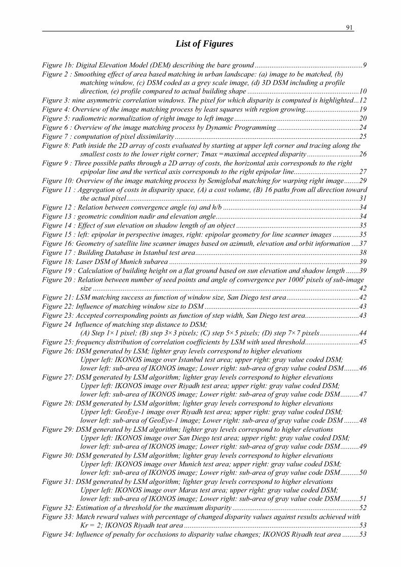
91

List of Figures

Figure 1b: Digital Elevation Model (DEM) describing the bare ground .......................................................... 9 Figure 2 : Smoothing effect of area based matching in urban landscape: (a) image to be matched, (b)

matching window, (c) DSM coded as a grey scale image, (d) 3D DSM including a profile direction, (e) profile compared to actual building shape ............................................................ 10 

Figure 3: nine asymmetric correlation windows. The pixel for which disparity is computed is highlighted ... 12 Figure 4: Overview of the image matching process by least squares with region growing ............................. 19 Figure 5: radiometric normalization of right image to left image ................................................................... 20 Figure 6 : Overview of the image matching process by Dynamic Programming ............................................ 24 Figure 7 : computation of pixel dissimilarity ................................................................................................... 25 Figure 8: Path inside the 2D array of costs evaluated by starting at upper left corner and tracing along the

smallest costs to the lower right corner; Tmax =maximal accepted disparity ............................ 26 Figure 9 : Three possible paths through a 2D array of costs, the horizontal axis corresponds to the right

epipolar line and the vertical axis corresponds to the right epipolar line ................................... 27 Figure 10: Overview of the image matching process by Semiglobal matching for warping right image ........ 29 Figure 11 : Aggregation of costs in disparity space, (A) a cost volume, (B) 16 paths from all direction toward

the actual pixel ............................................................................................................................. 31 Figure 12 : Relation between convergence angle (α) and h/b ......................................................................... 34 Figure 13 : geometric condition nadir and elevation angle ............................................................................. 34 Figure 14 : Effect of sun elevation on shadow length of an object .................................................................. 35 Figure 15 : left: epipolar in perspective images, right: epipolar geometry for line scanner images .............. 35 Figure 16: Geometry of satellite line scanner images based on azimuth, elevation and orbit information .... 37 Figure 17 : Building Database in Istanbul test area ........................................................................................ 38 Figure 18: Laser DSM of Munich subarea ...................................................................................................... 39 Figure 19 : Calculation of building height on a flat ground based on sun elevation and shadow length ....... 39 Figure 20 : Relation between number of seed points and angle of convergence per 10002 pixels of sub-image

size ............................................................................................................................................... 42 Figure 21: LSM matching success as function of window size, San Diego test area ....................................... 42 Figure 22: Influence of matching window size to DSM ................................................................................... 43 Figure 23: Accepted corresponding points as function of step width, San Diego test area ............................. 43 Figure 24 Influence of matching step distance to DSM;

(A) Step 1×1 pixel; (B) step 3×3 pixels; (C) step 5×5 pixels; (D) step 7×7 pixels ..................... 44 Figure 25: frequency distribution of correlation coefficients by LSM with used threshold ............................. 45 Figure 26: DSM generated by LSM; lighter gray levels correspond to higher elevations

Upper left: IKONOS image over Istanbul test area; upper right: gray value coded DSM; lower left: sub-area of IKONOS image; Lower right: sub-area of gray value coded DSM ........ 46 

Figure 27: DSM generated by LSM algorithm; lighter gray levels correspond to higher elevations Upper left: IKONOS image over Riyadh test area; upper right: gray value coded DSM; lower left: sub-area of IKONOS image; Lower right: sub-area of gray value code DSM .......... 47 

Figure 28: DSM generated by LSM algorithm; lighter gray levels correspond to higher elevations Upper left: GeoEye-1 image over Riyadh test area; upper right: gray value coded DSM; lower left: sub-area of GeoEye-1 image; Lower right: sub-area of gray value code DSM ........ 48 

Figure 29: DSM generated by LSM algorithm; lighter gray levels correspond to higher elevations Upper left: IKONOS image over San Diego test area; upper right: gray value coded DSM; lower left: sub-area of IKONOS image; Lower right: sub-area of gray value code DSM .......... 49 

Figure 30: DSM generated by LSM algorithm; lighter gray levels correspond to higher elevations Upper left: IKONOS image over Munich test area; upper right: gray value coded DSM; lower left: sub-area of IKONOS image; Lower right: sub-area of gray value code DSM .......... 50 

Figure 31: DSM generated by LSM algorithm; lighter gray levels correspond to higher elevations Upper left: IKONOS image over Maras test area; upper right: gray value coded DSM; lower left: sub-area of IKONOS image; Lower right: sub-area of gray value code DSM .......... 51 

Figure 32: Estimation of a threshold for the maximum disparity .................................................................... 52 Figure 33: Match reward values with percentage of changed disparity values against results achieved with

Kr = 2; IKONOS Riyadh teat area .............................................................................................. 53 Figure 34: Influence of penalty for occlusions to disparity value changes; IKONOS Riyadh teat area ......... 53 

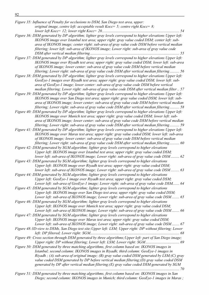
92

Figure 35: Influence of Penalty for occlusions to DSM, San Diego test area, upper: original image, centre left: acceptable result Kocc= 5; centre right Kocc= 8; lower left Kocc= 12; lower right Kocc= 20 ................................................................................ 54 

Figure 36: DSM generated by DP algorithm; lighter gray levels correspond to higher elevations Upper left: IKONOS image over Istanbul test area; upper right: gray value coded DSM; center left: sub-area of IKONOS image; center right: sub-area of gray value code DSM before vertical median filtering; lower left: sub-area of IKONOS image; Lower right: sub-area of gray value code DSM after vertical median filtering ............................................................................................ 55 

Figure 37: DSM generated by DP algorithm; lighter gray levels correspond to higher elevations Upper left: IKONOS image over Riyadh test area; upper right: gray value coded DSM; lower left: sub-area of IKONOS image; lower center: sub-area of gray value code DSM before vertical median filtering; Lower right: sub-area of gray value code DSM after vertical median filtering .......... 56 

Figure 38: DSM generated by DP algorithm; lighter gray levels correspond to higher elevations Upper left: GeoEye-1 images over Riyadh test area; upper right: gray value coded DSM; lower left: sub-area of GeoEye-1 image; lower center: sub-area of gray value code DSM before vertical median filtering; Lower right: sub-area of gray value code DSM after vertical median filter .. 57 

Figure 39: DSM generated by DP algorithm; lighter gray levels correspond to higher elevations Upper left: IKONOS image over San Diego test area; upper right: gray value coded DSM; lower left: sub-area of IKONOS image; lower center: sub-area of gray value code DSM before vertical median filtering; Lower right: sub-area of gray value code DSM after vertical median filtering .......... 58 

Figure 40: DSM generated by DP algorithm; lighter gray levels correspond to higher elevations Upper left: IKONOS image over Munich test area; upper right: gray value coded DSM; lower left: sub-area of IKONOS image; lower center: sub-area of gray value code DSM before vertical median filtering; Lower right: sub-area of gray value code DSM after vertical median filtering .......... 59 

Figure 41: DSM generated by DP algorithm; lighter gray levels correspond to higher elevations Upper left: IKONOS image over Maras test area; upper right: gray value coded DSM; lower left: sub-area of IKONOS image; lower center: sub-area of gray value code DSM before vertical median filtering; Lower right: sub-area of gray value code DSM after vertical median filtering .......... 60 

Figure 42: DSM generated by SGM algorithm; lighter gray levels correspond to higher elevations Upper left: IKONOS image over Istanbul test area; upper right: gray value coded DSM; lower left: sub-area of IKONOS image; Lower right: sub-area of gray value code DSM ......... 62 

Figure 43: DSM generated by SGM algorithm; lighter gray levels correspond to higher elevations Upper left: IKONOS image over Riyadh test area; upper right: gray value coded DSM; lower left: sub-area of IKONOS image; Lower right: sub-area of gray value code DSM ......... 63 

Figure 44: DSM generated by SGM algorithm; lighter gray levels correspond to higher elevations Upper left: GeoEye-1 image over Riyadh test area; upper right: gray value coded DSM; Lower left: sub-area of GeoEye-1 image; Lower right: sub-area of gray value code DSM ....... 64 

Figure 45: DSM generated by SGM algorithm; lighter gray levels correspond to higher elevations Upper left: IKONOS image over San Diego test area; upper right: gray value coded DSM; Lower left: sub-area of IKONOS image; Lower right: sub-area of gray value code DSM ........ 65 

Figure 46: DSM generated by SGM algorithm; lighter gray levels correspond to higher elevations Upper left: IKONOS image over Munich test area; upper right: gray value coded DSM; Lower left: sub-area of IKONOS image; Lower right: sub-area of gray value code DSM ........ 66 

Figure 47: DSM generated by SGM algorithm; lighter gray levels correspond to higher elevations Upper left: IKONOS image over Maras test area; upper right: gray value coded DSM; Lower left: sub-area of IKONOS image; Lower right: sub-area of gray value code DSM ........ 67 

Figure 48:3D-view to DSMs, San Diego test site;Upper left: LSM; Upper right: DP without filtering; Lower left: DP filtered; Lower right: SGM ............................................................................................ 68 

Figure 49: Cross section through DSM generated by three algorithms;Upper left: part of San Diego image; Upper right: DP without filtering; Lower left: LSM; Lower right: SGM ................................... 69 

Figure 50: DSM generated by three matching algorithms, first column based on: IKONOS images in Istanbul; second column: IKONOS images in Riyadh; third column: GeoEye-1 images in Riyadh ; (A) sub-area of original image; (B) gray value coded DSM generated by LSM;(C) gray value coded DSM generated by DP before vertical median filtering;(D) gray value coded DSM generated by DP after vertical median filtering;(E) gray value coded DSM generated by SGM ..................................................................................................................................................... 70 

Figure 51: DSM generated by three matching algorithms, first column based on: IKONOS images in San Diego; second column: IKONOS images in Munich; third column: GeoEye-1 images in Maras ;

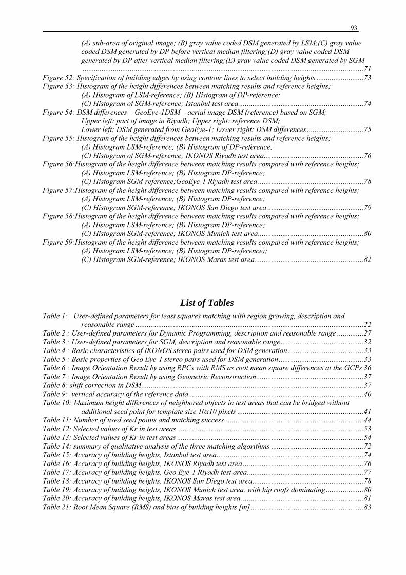
93

(A) sub-area of original image; (B) gray value coded DSM generated by LSM;(C) gray value coded DSM generated by DP before vertical median filtering;(D) gray value coded DSM generated by DP after vertical median filtering;(E) gray value coded DSM generated by SGM ..................................................................................................................................................... 71 

Figure 52: Specification of building edges by using contour lines to select building heights ......................... 73 Figure 53: Histogram of the height differences between matching results and reference heights;

(A) Histogram of LSM-reference; (B) Histogram of DP-reference; (C) Histogram of SGM-reference; Istanbul test area .................................................................. 74 

Figure 54: DSM differences – GeoEye-1DSM – aerial image DSM (reference) based on SGM; Upper left: part of image in Riyadh; Upper right: reference DSM; Lower left: DSM generated from GeoEye-1; Lower right: DSM differences .............................. 75 

Figure 55: Histogram of the height differences between matching results and reference heights; (A) Histogram LSM-reference; (B) Histogram of DP-reference; (C) Histogram of SGM-reference; IKONOS Riyadh test area..................................................... 76 

Figure 56:Histogram of the height difference between matching results compared with reference heights; (A) Histogram LSM-reference; (B) Histogram DP-reference; (C) Histogram SGM-reference;GeoEye-1 Riyadh test area ........................................................ 78 

Figure 57:Histogram of the height difference between matching results compared with reference heights; (A) Histogram LSM-reference; (B) Histogram DP-reference; (C) Histogram SGM-reference; IKONOS San Diego test area ................................................... 79 

Figure 58:Histogram of the height difference between matching results compared with reference heights; (A) Histogram LSM-reference; (B) Histogram DP-reference; (C) Histogram SGM-reference; IKONOS Munich test area ........................................................ 80 

Figure 59:Histogram of the height difference between matching results compared with reference heights; (A) Histogram LSM-reference; (B) Histogram DP-reference); (C) Histogram SGM-reference; IKONOS Maras test area.......................................................... 82 

List of Tables Table 1: User-defined parameters for least squares matching with region growing, description and

reasonable range ......................................................................................................................... 22 Table 2 : User-defined parameters for Dynamic Programming, description and reasonable range .............. 27 Table 3 : User-defined parameters for SGM, description and reasonable range ............................................ 32 Table 4 : Basic characteristics of IKONOS stereo pairs used for DSM generation ........................................ 33 Table 5 : Basic properties of Geo Eye-1 stereo pairs used for DSM generation ............................................. 33 Table 6 : Image Orientation Result by using RPCs with RMS as root mean square differences at the GCPs 36 Table 7 : Image Orientation Result by using Geometric Reconstruction ......................................................... 37 Table 8: shift correction in DSM ...................................................................................................................... 37 Table 9: vertical accuracy of the reference data ............................................................................................. 40 Table 10: Maximum height differences of neighbored objects in test areas that can be bridged without

additional seed point for template size 10x10 pixels ................................................................... 41 Table 11: Number of used seed points and matching success .......................................................................... 44 Table 12: Selected values of Kr in test areas ................................................................................................... 53 Table 13: Selected values of Kr in test areas ................................................................................................... 54 Table 14: summary of qualitative analysis of the three matching algorithms ................................................. 72 Table 15: Accuracy of building heights, Istanbul test area .............................................................................. 74 Table 16: Accuracy of building heights, IKONOS Riyadh test area ................................................................ 76 Table 17: Accuracy of building heights, Geo Eye-1 Riyadh test area .............................................................. 77 Table 18: Accuracy of building heights, IKONOS San Diego test area ........................................................... 78 Table 19: Accuracy of building heights, IKONOS Munich test area, with hip roofs dominating .................... 80 Table 20: Accuracy of building heights, IKONOS Maras test area ................................................................. 81 Table 21: Root Mean Square (RMS) and bias of building heights [m] ............................................................ 83 

94

Acknowledgements

I would like to thank several persons who supported and helped me with my investigations and

developments leading to this thesis.

First of all I am especially indebted to Prof. Dr. Martin Kappas from University of Göttingen who invited me

to study in Germany; I wish to express my deepest gratitude to him for the useful suggestions and support in

order to complete my research at IPI after nine months working with him at Cartography, GIS and Remote

Sensing Section.

When I came from Göttingen to Hannover in December 2005 to continue my thesis, at first I was afraid of

working with Prof. Heipke and his group, because I heard that he accepts only candidates with a very high

scientific level. But after short time he was able to integrate me into his group. My deepest gratitude goes to

my supervisor Prof. Dr.-Ing. Christian Heipke for supporting my work with his profound knowledge,

challenging questions, invaluable suggestions, and his precise reviews and the interesting discussions we

had. He enabled me to gain more experiences in my research field. Many thanks go to him for giving me the

opportunity to participate in international scientific conferences to present my research results.

Secondly, I want to thank Dr.-Ing. Karsten Jacobsen for continuing my supervision, for his invaluable

advices and fruitful discussions and help to detect some hidden errors in my thesis. Nothing I can say would

be enough to express my feelings and my deep appreciation to his valuable friendship besides his willingness

to help in every technical and personal aspect. I also truly appreciate Dr. Jacobsen patience during the thesis.

I would also like to thank Professor Martin Kappas and Professor Monika Sester for serving on my thesis

committee as examiners.

Special thanks are extended to Dr.-Ing. Franz Rottensteiner and Dr.-Ing. Ralph Schmidt for reading the thesis

and the support with enlightening advices.

I would like to acknowledge all my colleagues and friends from around the world who shared in my room at

IPI during their visit to IPI, especially Volker Lohse from Germany, Paula Redweik from Portugal, Badea

Dragos from Romania, Hidenori Fujimura from Japan, Mohammed Al Sayel from Saudi Arabia, Farhad

Goodarzi from Iran, Outi Klang from Finland and Abdelkader Elgarouani from Morocco. I wish them a lot

of success in their careers.

Many thanks to my colleagues at IPI who helped me in countless ways, all these years I enjoyed their

friendliness and good spirit. They are more than friends to me.

My final thanks to my father and mother for their understanding and their enduring patience during this very

trying period, I am in great debt to my wife and my children in taking a lot time from them to concentrate on

this study during these almost 6 years.

Many thanks to all of you and to those I miss…

Abdalla Alobeid

95

Curriculum Vitae

Applicant Last name, First name : Alobeid, Abdalla Birth date: 03.12.1973

Birthplace :Aleppo ,Syria

Nationality: Syrian

Marital Status: Married

Position: Dipl.-Eng.

Education Details 1993 : Final secondary school examinations, Aleppo ,Syria 1993-1999: Bachelor degree in field of specialization in Topography, Faculty of Civil Engineering,

Aleppo University, Syria. (B.Sc. Eng.) B.Sc. Ing.Thesis:

Monitoring Vertical and Horizontal Deformations in residential buildings, Faculty of Civil Engineer- ing, Aleppo University, Syria,1999

Dipl.-Eng. Thesis: I. 3D-Documentation of Archaeological Buildings in Aleppo by Digital Photogrammetry, Faculty of

Civil Engineering, Aleppo University, Syria,2004 II. Generation and analyses of digital surface models in urban areas based on aerial images, Institute of

Photogrammetry and GeoInformation (IPI), Leibniz University Hannover, Germany, 2006

1999-2002: Surveying engineer at General Organization of Surveying in Aleppo 2003-2004: Scholarship to obtain the Diploma of Higher Studies in Topography for the General

Organization of Remote Sensing (GORS), Aleppo University. (Dipl.-Eng.) 2004-2005: PhD candidate at the Institute of Geography, University of Gottingen, Germany (Prof. Dr.

Martin Kappas) Since 2006: PhD candidate at the Institute of Photogrammetry and GeoInformation (IPI), Leibniz

University Hannover, Germany

96

List of Publications

Alobeid, A., Jacobsen, K., Heipke, C, M. Al Rajhi,, 2011: Building Monitoring with Differential DSMs, International Archives of Photogrammetry, Remote Sensing and Spatial Information Sciences Volume XXXVIII-4/W 19, Hannover, 12 pages, CD available at : www.ipi.uni-hannover.de (last accessed: Juli 2011) Jacobsen, K., Alobeid, A., 2011:

Monitoring of Buildings based on GeoEye-1, IKONOS and aerial image stereo pairs, 31 EARSel symposium 2011 in Prague, Czech Republic , 8 S., CD available at : http://www.conferences.earsel.org/abstract/show/2375 : www.ipi.uni-hannover.de (last accessed: Juli 2011) Alobeid, A., Jacobsen, K., Heipke, C, 2010:

Comparison of Matching Algorithms for DSM Generation in Urban Areas from Ikonos Imagery, Photogrammetric Engineering & Remote Sensing, 76(9). pp. 1041-1050 Jacobsen, K., Alobeid, A., 2010:

Digital Surface Models in Urban Areas based on Satellite Imagery: EARSeL Workshop, Gent, 10 S., CD available at : www.ipi.uni-hannover.de (last accessed: Juli 2011) Sefercik, U. G., Alobeid, A., Soergel, U., Jacobsen, K., 2010:

Generation and Analysis of DEMs Based on Space-Borne Remote Sensing, 17th International Symposium. Damascus, CD, 6 S. available at : www.ipi.uni-hannover.de (last accessed: Juli 2011) Alobeid, A., Jacobsen, K., Heipke, C., 2009:

Building Height Estimation in Urban Areas from Very High Resolution Satellite Stereo Images: International Archives of Photogrammetry, Remote Sensing and Spatial Information Sciences (38), Part 1-4-7/WS, Hannover, 6 pages, CD available at : www.ipi.uni-hannover.de (last accessed: Juli 2011) Alobeid, A., Jacobsen, K., 2008:

Generation and analysis of digital surface models in urban areas based on aerial images: International Archives of Photogrammetry, Remote Sensing and Spatial Information Sciences XXXVII, Part B4. Peking, S. 1207-1212. available at : www.ipi.uni-hannover.de (last accessed: Juli 2011) Alobeid, A., Jacobsen, K., 2008:

Automatic generation of digital surface models from Ikonos stereo imagery and related application: GORS, 16th International Symposium. Damascus, CD, 8 pages available at : www.ipi.uni-hannover.de (last accessed: Juli 2011)

Wissenschaftliche Arbeiten der Fachrichtung Geodäsie und Geoinformatik der Leibniz Universität Hannover

Die Arbeiten werden im Rahmen des wissenschaftlichen Schriftenaustausches verteilt und sind nicht im Buchhandel erhältlich. Der Erwerb ist zu einem Stückpreis von € 25,-- bei den herausgebenden Instituten möglich.

(Eine vollständige Liste der Wiss. Arb. ist beim Geodätischen Institut, Nienburger Str. 1, 30167 Hannover erhältlich.) Nr. 265 RAGUSE, Karsten: Dreidimensionale photogrammetrische Auswertung asynchron aufgenommener

Bildsequenzen mittels Punktverfolgungsverfahren (Diss. 2007) Nr. 266 HAMPE, Mark: Integration einer multiskaligen Datenbank in eine Webservice-Architektur (Diss. 2007) Nr. 267 ANDERS, Frauke: Mustererkennung in Straßennetzwerken - Verfahren zur Interpretation von Vektordaten. (Diss. 2007) Nr. 268 HESSE, Christian: Hochauflösende kinematische Objekterfassung mit terrestrischen Laserscannern (Diss. 2007) Nr. 269 NEUNER, Zur Modellierung und Analyse instationärer Deformationsprozesse (Diss. 2007) Hans-Berndt: Nr. 270 WENDT, Axel: Objektraumbasierte simultane multisensorale Orientierung (Diss. 2007) Nr. 271 DILßNER, Florian: Zum Einfluss des Antennenumfeldes auf die hochpräzise GNSS- Positionsbestimmung (Diss. 2007) Nr. 272 BUTENUTH, Network Snakes (Diss. 2008) Matthias: Nr. 273 RAVANBAKHSH, Road Junction Extraction from High Resolution Aerial Images Assisted by Mehdi: Topographic Database Information (Diss. 2008) Nr. 274 BRZANK, Bestimmung Digitaler Geländemodelle in Wattgebieten aus Laserscannerdaten Alexander: (Diss. 2008) Nr. 275 SCHMIDT, Ralph: Automatische Bestimmung von Verknüpfungspunkten für HRSC-Bilder der

Mars Express-Mission (Diss. 2008) Nr. 276 HAUNERT, Aggregation in Map Generalization by Combinatorial Optimization (Diss. 2008) Jan-Henrik: Nr. 277 NEUMANN, Ingo: Zur Modellierung eines erweiterten Unsicherheitshaushaltes in Parameterschätzung und Hypothesentests (Diss. 2009) Nr. 278 WEITKAMP, Brachflächenrevitalisierung im Rahmen der Flächenkreislaufwirtschaft Alexandra: (Diss. 2009) Nr. 279 HEUWOLD, Janet: Automatische auflösungsabhängige Anpassung von Bildanalyse-Objektmodellen

am Beispiel Straßen (Diss. 2009) Nr. 280 KOCH, Christian: Extraction of Mercury's tidal signal and libration amplitude from synthetic

laser altimeter data sets (Diss. 2009) Nr. 281 GITLEIN, Olga: Absolutgravimetrische Bestimmung der Fennoskandischen Landhebung mit dem FG5-220 (Diss. 2009) Nr. 282 ELING, Dirk: Terrestrisches Laserscanning für die Bauwerksüberwachung (Diss. 2009) Nr. 283 DOLD, Christoph: Ebenenbasierte Verfahren für die automatische Registrierung terrestrischer Laserscans (Diss. 2010) Nr. 284 RIPPERDA, Nora: Rekonstruktion von Fassadenstrukturen mittels formaler Grammatiken und Reversible Jump Markov Chain Monte Carlo Sampling (Diss. 2010) Nr. 285 KATTERFELD Interoperables Geodaten-basiertes E-Learning (Diss. 2010) Christiane: Nr. 286 JARECKI, Focke: Spurkreuzungspunktdifferenzen zur Validierung satellitengradiometrischer Messungen (Diss. 2010) Nr. 287 SCHRAMM, Unüberwachte lineare spektrale Entmischung mit Anwendungen für Matthias: Baumdichteabschätzungen in semiariden Regionen Afrikas (Diss. 2010) Nr. 288 ALSAYEL, Towards Standardizing International Boundary Determination and Quality Mohammed Y.: Consequences on surveying and Mapping (Diss. 2010) Nr. 289 TAVAKKOLI S., Multi-Temporal Classification of Crops Using ENVISAT ASAR Data Seyed Mohammad: (Diss. 2011) Nr. 290 VENNEGEERTS, Objektraumgestützte kinematische Georeferenzierung für Mobile-Mapping- Harald: Systeme (Diss. 2011) Nr. 291 BULATOV, Dimitri: Textured 3D reconstruction of urban terrain from UAV-borne video sequences (Diss. 2011) Nr. 292 GROTE, Anne: Automatic road network extraction in suburban areas from aerial images (Diss. 2011) Nr. 293 ALOBEID, Abdalla: Assessment of Matching Algorithms for Urban DSM Generation from Very High Resolution Satellite Stereo Images (Diss. 2011)