Nuclear matter in the crust of neutron stars

PHYSICAL REVIEW C 76, 024312 (2007)

Nuclear matter in the crust of neutron stars

P. Gogelein and H. MutherInstitut fur Theoretische Physik, Universitat Tubingen, D-72076 Tubingen, Germany

(Received 19 April 2007; published 13 August 2007)

The properties of inhomogeneous nuclear matter are investigated considering the self-consistent Skyrme-Hartree-Fock approach with inclusion of pairing correlations. For a comparison we also consider a relativisticmean-field approach. The inhomogeneous infinite matter is described in terms of cubic Wigner-Seitz cells, whichleads to a smooth transition to the limit of homogeneous nuclear matter. The possible existence of variousstructures in the so-called pasta phase is investigated within this self-consistent approach and a comparison ismade to results obtained within the Thomas-Fermi approximation. Results for the proton abundances and thepairing properties are discussed for densities for which clustering phenomena are obtained.

DOI: 10.1103/PhysRevC.76.024312 PACS number(s): 21.60.Jz, 21.65.+f, 26.60.+c, 97.60.Jd

I. INTRODUCTION

The crust of neutron stars is a very intriguing objectfor theoretical nuclear structure physics, as it contains thetransition from stable nuclei in the outer crust to a system ofhomogeneous nuclear matter, consisting of protons, neutrons,and leptons in β equilibrium, in the inner part of this crust.The question of how matter consisting of isolated nuclei meltsinto uniform matter with increasing density has evoked a largenumber of studies [1–4]. Already at moderate densities theFermi energy of the electron is so high that the β stabilityenhances the neutron fraction of the baryons so much thata part of these neutrons drip out of the nuclei. This leadsto a structure in which quasinuclei, clusters of protons andneutrons, are embedded in a sea of neutrons. To minimize theCoulomb repulsion between the protons, the quasinuclei forma lattice.

Therefore one typically describes these structures in formof the Wigner-Seitz (WS) cell approximation. One assumesa geometrical shape for the quasinuclei and determines thenuclear contribution to the energy of such a WS cell from aphenomenological energy-density functional. Such Thomas-Fermi (TF) calculations yield a variety of structures: Sphericalquasi-nuclei, which are favored at small densities, mergewith increasing density to strings, which then may cluster toparallel plates and so on. These geometrical structures havebeen the origin for the popular name of this phase: pastaphase.

Such Thomas-Fermi calculations, however, are very sensi-tive to the surface tension under consideration. Furthermorethey do not account for characteristic features of the structureof finite nuclei, like the shell effects. Shell effects favor theformation of closed-shell systems and may have a significanteffect on the formation of inhomogeneous nuclear structures inthe crust of neutron stars. These shell effects are incorporatedin self-consistent Hartree-Fock or mean-field calculations,which can treat finite nuclei, infinite matter, and inhomoge-neous structures in between within a consistent frame basedon an effective nucleon-nucleon interaction. Such calculationsemploying the density-dependent Skyrme forces [5,6] weredone more than 25 years ago by Bonche and Vautherin [7] andby a few other groups.

These studies show indeed that shell effects have asignificant influence on details like the proton fraction of thebaryonic matter in the inhomogeneous phase [8]. They alsoprovide the basis for a microscopic investigation of propertiesbeyond the equation of state. This includes the study of pairingphenomena, excitation modes, and response functions as wellas the effects of finite temperature.

Self-consistent Hartree-Fock calculations for such inho-mogeneous nuclear structures have typically been performedassuming a WS cell of spherical shape. This assumption ofquasinuclei with spherical symmetry reduces the numericalwork-load considerably. However, it does not allow theexploration of quasinuclear clusters in form of strings or platesas predicted from Thomas-Fermi calculations. Furthermorethe limit of homogeneous matter cannot be described in asatisfactory manner in such a spherical WS cell. Employingthe representation of plane wave single-particle states in termsof spherical Bessel functions leads to a density profile, which,depending on the boundary condition chosen, exhibits either aminimum or a maximum at the boundary of the cell. Bouncheand Vautherin [7] therefore suggested using a mixed basis,for which, depending on the angular momentum, differentboundary conditions were considered. However, even thisoptimised choice leads to density profiles with fluctuations [8].

Therefore the investigations presented here consider cubicWS cells, which allows for the description of nonsphericalquasinuclear structures and contains the limit of homogeneousmatter in a natural way. Self-consistent Hartree-Fock calcula-tions are performed for β-stable matter at densities for whichthe quasinuclear structures discussed above are expected. Forthe nuclear Hamiltonian we consider various Skyrme forcesbut also perform calculations within the effective relativisticmean-field approximation. Special attention will be paid tothe comparison between results obtained in the Hartree-Fockapproach and corresponding Thomas-Fermi calculations.

After this introduction we will briefly review the Hartree-Fock approximation using Skyrme interactions and the tech-nique used to solve the equations resulting from this approachemploying the imaginary time step method in Sec. II. Wethen turn to the relativistic mean-field approach and theadaption of the imaginary time step method to be used within

0556-2813/2007/76(2)/024312(12) 024312-1 ©2007 The American Physical Society

http://dx.doi.org/10.1103/PhysRevC.76.024312

P. GOGELEIN AND H. MUTHER PHYSICAL REVIEW C 76, 024312 (2007)

this relativistic framework. After a short description on theinclusion of pairing correlations in Sec. IV, we present resultsin Sec. V. The main conclusions are summarized in Sec. VI.

II. SKYRME-HARTREE-FOCK CALCULATIONS

A. Energy functional

The Skyrme-Hartree-Fock (SHF) approach has frequentlybeen described in the literature [5–7,9]. Therefore we willrestrict the presentation here to a few basic equations, whichwill define the nomenclature. The Skyrme model is definedin terms of an energy density H(r), which can be split intovarious contributions [6,10]

H = HK + H0 + H3 + Heff + Hfin + Hso + HCoul, (1)

where HK is the kinetic energy term, H0 a zero-range term,H3 a density-dependent term, Heff an effective mass term, Hfin

a finite-range term, and Hso a spin-orbit term. These terms aregiven by

HK = h2

2mτ,

H0 = 14 t0

[(2 + x0)ρ2 − (2x0 + 1)

(ρ2

p + ρ2n

)],

H3 = 124 t3ρ

α[(2 + x3)ρ2 − (2x3 + 1)

(ρ2

p + ρ2n

)],

Heff = 18 [t1(2 + x1) + t2(2 + x2)]τρ + 1

8 [t2(2x2 + 1)(2)− t1(2x1 + 1)](τpρp + τnρn),

Hfin = − 132 [3t1(2 + x1) − t2(2 + x2)]ρ�ρ + 1

32 [3t1(2x1 + 1)

+ t2(2x2 + 1)](ρp�ρp + ρn�ρn),

Hso = − 12W0(ρ∇ J + ρp∇ Jp + ρn∇ Jn).

The coefficients ti , xi,W0, and α are the parameters of ageneralized Skyrme force [11]. The energy density of Eq. (1)contains furthermore the contribution of the Coulomb force,HCoul, which is calculated from the charge density ρC as

HCoul = e2

2ρC(r)

∫d3r ′ ρC(r ′)

|r − r ′| − 3e2

4

(3

π

)1/3

ρ4/3C . (3)

Here the exchange part of the Coulomb term is calcu-lated within the Slater approximation. Following Ref. [11]the center-of-mass recoil energy has been approximated as−∑

p2i /2Am.

The densities ρ, τ , and J are defined in terms of thecorresponding densities for protons and neutrons ρ = ρp +ρn, τp + τn and J = Jp + Jn. If we identify the isospinlabel (q = n, p), the corresponding matter densities are givenby

ρq(r) =∑k,s

ηq

k

∣∣ϕq

k (r, s)∣∣2

, (4)

where ϕq

k (r, s) is the single-particle wave function with orbital,spin and isospin quantum numbers k, s, and q. The occupationfactors η

q

k are determined by the Fermi energy and the desiredscheme of occupation (see discussion below). The kinetic

energy and spin-orbit densities are defined by

τq(r) =∑k,s

ηq

k

∣∣∇ϕq

k (r, s)∣∣2

, (5)

Jq(r) = −i∑k,s,s ′

ηq

k

(ϕ

q

k

)∗(r, s ′) ∇ϕ

q

k (r, s) × 〈s ′|σ |s〉. (6)

The gradient of the spin-orbit density ∇ J = ∇ Jp + ∇ Jn canbe directly evaluated without first calculating J :

∇ Jq(r) = −i∑k,s,s ′

ηq

k ∇(ϕ

q

k

)∗(r, s ′) × ∇ϕ

q

k (r, s) · 〈s ′|σ |s〉.

(7)

We left out the spin-gradient term [10], which is cumbersometo evaluate in three-dimensional calculations numerically andnot very important.

The single-particle wave functions are determined assolutions of the Hartree-Fock equations[

−∇ h2

2m∗q(r)

∇ + Uq(r) − iW q(r) · (∇ × σ )

]ϕ

q

k (r)

= εq

k ϕq

k (r, s), (8)

with an effective mass term m∗(r), which depends on the Heff

part of the energy-density functional

h2

2m∗q(r)

= h2

2m+ 1

8 [t1(2 + x1) + t2(2 + x2)] ρ(r)

+ 18 [t2(1 + 2x2) − t1(1 + 2x1)] ρq(r), (9)

a nuclear central Potential

Uq(r) = 12 t0[(2 + x0)ρ − (1 + 2x0)ρq]

+ 124 t3(2 + x3)(2 + α)ρα+1 − 1

24 t3(2x3 + 1)

× [2ραρq + αρα−1

(ρ2

p + ρ2n

)] + 18 [t1(2 + x1)

(10)+ t2(2 + x2)]τ + 1

8 [t2(2x2 + 1) − t1(2x1 + 1)]τq

+ 116 [t2(2 + x2) − 3t1(2 + x1)]�ρ

+ 116 [3t1(2x1 + 1) + t2(2x2 + 1)]�ρq

− 12W0(∇ J + ∇ Jq) + δq,pVCoul

with the Coulomb field

VCoul(r) = e2∫

d3r ′ ρC(r ′)|r − r ′| − e2

(3

π

)1/3

ρ1/3C (11)

and a spin-orbit field:

W q(r) = 12W0(∇ρ + ∇ρq). (12)

B. Imaginary time step

Various different methods have been developed to solve theHartree-Fock equations. Frequently the single-particle wavefunctions are expanded in a basis like, e.g., the eigenfunctionsof an appropriate harmonic oscillator. This is appropriate fordescribing the wave functions for single-particle states, whichare deeply bound. It is not so appropriate for the description ofweakly bound or unbound single-particle states, because the

024312-2

NUCLEAR MATTER IN THE CRUST OF NEUTRON STARS PHYSICAL REVIEW C 76, 024312 (2007)

asymptotic behavior of the harmonic oscillator basis states isnot appropriate for these states.

This can be cured by employing the eigenstates of aspherical box with an appropriate radius R [8], which can alsobe considered as a WS cell for describing periodic systems.Such a spherical box, however, is not appropriate for thedescription of deformed nuclei and nuclear structures as theyare expected for the pasta phase in the crust of neutron stars.This, as well as the problems with the boundary conditions ina spherical WS cell discussed already in the introduction, callsfor a Cartesian WS cell.

The single-particle wave functions in such a cartesianWS cell can be represented by its values on a discretizedmesh in this cell. The spacings between the mesh points,�x,�y, and �z correspond to truncations in momentumspace. Smaller values for these spacings account for largermomentum components in the wave functions. The obviousdisadvantage of such calculations is the huge amount of meshpoints that has to be taken into account. Therefore one needsa fast iterative procedure for the solution of the self-consistentHartree-Fock (HF) equations, which evaluates only the desiredstates.

Davies et al., presented in Ref. [12] an efficient method forthis problem, the imaginary time step method, which we wantto outline briefly. The origin for the name of this method is theanalogy to the time-dependent Hartree-Fock (TDHF) methodthat solves the equations

ih∂ϕk

∂t= H (t)ϕk(t), k = 1, . . . , A, (13)

for an orthonormal set of A wave functions {ϕk}, and aHamiltonian H that depends on the time t . This is thecase when we identify H (t), e.g., with the HF Hamiltonianrepresented in Eq. (8), that depends on t as it depends on theresulting wave function ϕk(t) in a self-consistent way. Theseequations are discretized in time introducing a time step �t ,with tn = n�t . Then the time evolution of the set of wavefunctions {ϕk} may be approximated by the iterative procedure∣∣ϕ(n+1)

k

⟩ = exp

(− i

h�tH (n+ 1

2 )

) ∣∣ϕ(n)k

⟩, k = 1, . . . , A, (14)

in which ϕ(n)k represents the wave function ϕk at the time

tn and H (n+ 12 ) denotes the numerical approximation to the

Hamiltonian H (t) at the time (n + 12 )�t . The idea of Davies

et al., was to replace the time step �t by the imaginaryquantity −i�t . Introducing the positive parameter λ = �t/h

the procedure for the imaginary time step gets∣∣ϕ(n+1)k

⟩ = exp( − λH (n+ 1

2 ))∣∣ϕ(n)

k

⟩, k = 1, . . . , A, (15)

where {ϕ(n+1)k } is no longer an orthonormal set of wave

functions because the imaginary time operator exp(−λH (n+ 12 ))

is not unitary. Applying the Gram-Schmidt orthonormalizationmethod O we get the orthonormal set {ϕ(n+1)

k } by∣∣ϕ(n+1)k

⟩ = O∣∣ϕ(n+1)

k

⟩k = 1, . . . , A. (16)

This procedure converges leading to those eigenfunctionsof the Hamiltonian H , which correspond to the lowest A

eigenvalues of the Hamiltonian H .

In practical applications the Hamiltonian H (n+ 12 ) is replaced

by the Hamiltonian H (n) of the n-th step, which makesthe calculation fast keeping the algorithm stable. After thisreplacement, we get the following operation on the wavefunctions

ϕ(n+1)k = O

[exp(−λH (n))ϕ(n)

k

]k = 1, . . . , A. (17)

For numerical application one has to truncate the exponentialseries to a certain order. In earlier HF calculations thegradient method was used with the operation O(1 − λH )on the wave functions [9]. If one truncates the exponentialseries in the imaginary time step going beyond the firstorder one obtains an improvement of the gradient method.Davies et al. recommended a truncation to fourth or fifthorder for a HF calculation of 40Ca together with a time step�t = 4.0 × 10−24 s and a mesh size of 1.0 fm.

In our calculations we used the same mesh size as Davieset al. but the convergence got worse because we consider inour studies a larger number of nucleons, which implies a largernumber of wave functions A have to be evolved. Hence wetruncated the exponential operator at ninth order and the timestep �t was set to 2.0 × 10−24s. For the check of convergencethe mean square deviation of the single-particle energies forN Nucleons and ηk the occupation probability is calculated by

�H (n) =[

1

N

A∑k=1

ηk

(⟨ϕ

(n)k

∣∣H (n)2 ∣∣ϕ(n)k

⟩ − ⟨ϕ

(n)k

∣∣H (n)∣∣ϕ(n)

k

⟩2)] 12

,

(18)

which provides a better criterion as calculating energy differ-ences.

The HF equations have been solved by discretization incoordinate space within a cubic Wigner-Seitz cell similar tothat used in Ref. [11] with periodic boundary conditions. Thebox sizes typically considered vary from 2 × 10 fm to 2 ×16 fm. This technique is able to allow for general deformationsof the quasinuclear structures. The densities we are consideringrequires accounting for around 1500 nucleons, which impliesthat up to A = 2600 wave functions had to be evolved toaccount for pairing correlations with occupation probabilitiesηk different from zero.

To decrease the numerical effort we assume two symmetrieslike in Ref. [11]:

(i) parity

P ϕk(r, s) = ϕk(−r, s) = pkϕk(r, s), pk = ±1; (19)

(ii) z signature

exp{iπ

(Jz − 1

2

)}ϕk(x, y, z, s)

= σϕk(−x,−y, z, s) = ηkϕk(x, y, z, s),(20)

ηk = ±1.

These symmetries still allow triaxial deformations andreduce the calculation to the positive coordinates in eachdirection. As additional symmetry time-reversal-invariance isassumed for the time-reversed pairs ϕk , and ϕk:

ϕk(r, s) = (T ϕk)(r, s) = σϕ∗k (r,−s). (21)

024312-3


TABLE I. Parity properties of the Pauli spinorswith respect to the coordinate planes.

x = 0 y = 0 z = 0

Re ϕk(r, + 12 ) + + pk

Im ϕk(r, + 12 ) − − pk

Re ϕk(r, − 12 ) − + −pk

Im ϕk(r, − 12 ) + − −pk

Summarizing this symmetries it is sufficient to solve the HFequations for one wave function of the time-reversed pairs.We choose the positive z-signature orbital for which we getthe symmetries summarized in Table I. The wave functionsϕk(r, s) are realized as complex Pauli spinors. The reflectionsat the x = 0 and y = 0 planes are realized by the parityoperator of the real part together with complex conjugation.

The iteration is performed with accurate numerical meth-ods. For the differential operators 11-point formulas are used,which have been derived by eliminating errors for functionsf with f (x) = xn up to a certain n0 ∈ N. The ansatz for thenumerical approximation of the derivatives on an equidistantmesh with the points xi and fi = f (xi) is for the first derivative

∂

∂xf (xi) ≈

(∂

∂x

)num

f (xi) =N∑

j=1

aj

1

2j�x(fi+j − fi−j ),

(22)

with N = 5 for 11-point formula and aj the coefficients of theformula. Requiring that the approximation gets equal up to acertain n0 ∈ N we obtain a linear equation. Inserting the resultin the ansatz we finally obtain(

∂

∂x

)num

f (xi)

= 1

�x

[1

19860(11fi+5 − 4500fi+2 + 16350fi+1

− 16350fi−1 + 4500fi−2 − 11fi−5) + 1

55608(−445fi+4

+ 2950fi+3 − 2950fi−3 + 445fi−4)

]. (23)

For the second derivative used in the Laplacian the ansatz is

∂

∂xf (xi) ≈

(∂

∂x

)num

f (xi)

=N∑

j=1

aj

1

(j�x)2(fi+j − 2fi + fi−j ). (24)

and finally the formula gets(∂2

∂x2

)num

f (xi)

= 1

(�x)2

[1

49650(11fi+5 − 11250fi+2 + 81750fi+1

+ 81750fi−1 − 11250fi−2 + 11fi−5) − 1729639

595800fi

+ 1

333648(−1335fi+4 + 11800fi+3 + 11800fi−3

− 1335fi−4)

]. (25)

In the case of the WS cell calculations charge neutrality isassumed and electrons are taken into account as relativisticFermi gas that contributes to the charge density ρC(r) =ρp(r) − ρe. For the calculation of finite nuclei the electronsare not taken into account (ρe = 0).

There are different methods to solve the Poisson equation

− �VC(r) = 4πρc(r). (26)

It turned out that the numerically most accurate and stablemethod is the integration applying the Green’s function forthis problem

VC(r) =∫

V

dr ′3ρC(r ′)1

|r − r ′| . (27)

Unfortunately, this integral has lots of singularities, but it canbe rewritten. First, the Green’s function is written as [13]:

1

|r − r ′| = 12�r ′ |r − r ′|. (28)

Then the integral is transformed by Green’s theorem for scalarfunctions f and g defined on a Volume V with closed surfaceA = ∂V [14]:∫

V

dV (f �g) −∫

V

dV (g�f ) =∮

A=∂V

dA · (f ∇g − g∇f ).

(29)

Identifying and f = ρC(r ′) and g = 12 |r − r ′| the final result

gets

VC(r) = 1

2

∫V

dr ′3�ρC(r ′)|r − r ′| + 1

2

∮A=∂V

dA

× [ρC(r ′)∇r ′ |r − r ′| − |r − r ′|∇r ′ρC(r ′)], (30)

which has no singularities. Altogether the result of thistransformation behaves very well in numerical calculationsand the numerical result is practically the same as the exact one.For finite nuclei it is possible to drop the boundary integralsas has already been discussed by Vautherin [13].

We tested the computer program for the parameter setSkyrme III by comparing results for finite nuclei with thoseof Ref. [11]. Additional tests have been performed using theparameter set SLy4 [10].

III. RELATIVISTIC MEAN-FIELD CALCULATIONS

To test the sensitivity of the results on the model underconsideration we also investigated the quasinuclear structuresin the crust of neutron stars employing the relativistic mean-field approach in a cubic box.

A. From the Lagrangian to the Dirac equation

The relativistic mean-field approach is based on aLagrangian is similar to that in Ref. [15] and consists of three

024312-4


parts: Lagrangian for the free baryons LB , the free mesons LM

and the interaction Lagrangian Lint:

L = LB + LM + Lint, (31)

which take the form

LB = �(iγµ∂µ − m

)�,

LM = 1

2

(∂µ�σ∂µ�σ − m2

σ�2σ

)− 1

2

∑κ=ω,ρ,γ

[1

2F (κ)

µν − m2κA

(κ)µ A(κ)µ

], (32)

Lint = −�gσ�σ� − �gωγµA(ω)µ�

− �1

2gργµτ A(ρ)µ� − �eγµ

1

2(1 + τ3)A(γ )µ�,

with the field-strength tensor F (κ)µν = ∂µA(κ)

ν − ∂νA(κ)µ , the

meson fields �σ ,A(ω), A(ρ), and the electromagnetic fieldA(γ ). The bold symbols are isovectors, the γ µ are the Diracγ matrices, and � is a nucleon field that consistsof Dirac four-spinors with isospin space. The massesare the baryon mass m = 938.9 MeV and the me-son masses mσ = 520 MeV,mω = 783 MeV, and mρ =770 MeV according to a parameter set for the linearmodel from Horowitz and Serot [16] cited as L-HS inRef. [15]. The coupling constants of this parameter setare gσ = 10.4814, gω = 13.8144, and gρ = 8.08488. Thecharge of the electron e = √

αhc/4π where α is the finestructure constant and hc = 197.32 MeV fm.

Applying the equations of motion and taking the staticlimit we obtain in the Hartree approximation the static Diracequation [17]

εαψα = [α p + V + β(m − S)]ψα, (33)

where α and β are matrices like in Ref. [18], εα the single-particle energy of the state ψα, p the momentum operator, andS and V the the scalar and vector fields

S = −gσ�σ(34)

V = gωA(ω)0 + 1

2gρτ3A(ρ)0 + e 1

2 (1 − τ3)A(γ )0 .

For the mesons fields we get Klein-Gordan equations. Afterneglecting retardation effects and taking the Hartree approxi-mation the meson-field equations read(−� + m2

σ

)�σ = −gσρs(−� + m2

ω

)A

(ω)0 = gωρ

(35)(−� + m2ρ

)A

(ρ)0 = 1

2gρρ3

−�A(γ )0 = eρC

with the scalar density ρs , the baryon density ρ. The densitiesare calculated taking into account only the occupied positiveenergy states in the Fermi sea and neglecting the negativeenergy states in the Dirac sea (“no sea” approximation)

ρs =N∑

α=1

ηαψαψα

ρ =N∑

α=1

ηαψαγ0ψα

ρ3 =N∑

α=1

ηαψατ3γ0ψα

ρC =N∑

α=1

ηα ψα

1

2(1 − τ3)γ0ψα(−ρe),

where ηα are the occupation numbers determined by the BCSformalism. The electron density ρe has been considered forthe WS cell calculations but not for studies of finite nuclei.

B. Solving the triaxial Dirac equation

The solution of the Dirac equation for nucleons in a cubicbox differs of course in some aspects from that in the sphericalone. Therefore we briefly outline the numerical solution in thefollowing.

We decompose ψα in an upper and lower component Paulispinor:

ψα =(

ϕα

χα

). (36)

Hence after applying the transformation εα → εα − m toenergy levels without rest-mass the Dirac equation becomes

εαϕα = σ pχα + Uϕϕα(37)

εαχα = σ pϕα + Uχχα

with the potentials

Uϕ = −S + V(38)

Uχ = −2m + S + V.

Now we obtain an “effective Schroedinger equation” byinserting the lower component into the equation for the upperone. This method is according to Reinhard [15] the mostefficient way to solve the Dirac equation. First we modifythe lower component

(εα − Uχ )χα = σ pϕα (39)

and then we introduce an “effective mass term” that dependson the wave function

Bα = 1

εα − Uχ

(40)

and finally get the “effective Schroedinger equation”

εαϕα = σ pBα σ pϕα + Uϕϕα. (41)

So far the procedure corresponds to the method employedin calculations assuming spherical symmetry [19]. Using thediscretization in a Cartesian box, however, requires a differenttreatment of angular momentum and spin-orbit terms. Withthe help of the following formula for vector fields A and Bcommuting with σ

σAσB = AB + iσ (A × B) (42)

024312-5


we obtain from the relativistic kinetic energy term

σ pBασ pϕα = −∇Bα∇ϕα − i(∇Bα) · (∇ × σ )ϕα, (43)

which is like the nonrelativistic kinetic energy term plusthe spin-orbit term for the upper component. From a furthermodification we obtain an expression called “effective Hamil-tonian” ready for implementation

Hϕ,αϕα = −Bα�ϕα − (∇Bα) · (∇ϕα) − i(∇Bα) · (∇ × σ )ϕα

+Uϕϕα. (44)

To calculate the eigenvalue εα we cannot use the “effectiveHamiltonian” like a normal Hamiltonian because we have totake into account the effects of the lower component. This wedo in the following manner:

χα = Bασ pϕα (45)

and hence the next approximation of the eigenvalue ε(n+1)α in

the iteration scheme gets

ε(n+1)α =

∫d3r

(ϕ∗

αHϕ,αϕα + ε(n)α χ∗

αχα

). (46)

This means that in the lower component the whole newinformation is contained in the new Pauli spinor. The totalbinding energy is calculated like in Ref. [20] using Cartesiancoordinates

E =∑

α

ηαεα − 1

2

∫d3r

[− gσ�σ (r)ρs(r) + gωA

(ω)0 ρ(r)

+ 1

2gρA

(ρ)0 ρ3(r) + eA

(γ )0 ρC(r)

]+ Ecm + Epair (47)

with a center-of-mass correction in the case of finite nuclei

Ecm = − 34hω with hω = 41A−1/3 MeV (48)

in compliance with Ref. [21] and a pairing energy Epair

described in the next section.For the variation of the wave functions in the cubic box we

employ once more the imaginary time step in the followingmanner. First we operate on the upper component with theimaginary time step and the “effective Hamiltonian”:

ϕ(n+1)α = exp(−λHϕ,α)ϕ(n)

α (49)

and then the lower component is calculated:

χ (n+1)α = Bα σ pϕ(n+1)

α (50)

and finally both components are orthonormalized togethervia the Gram-Schmidt method considering the symmetriesof the Dirac spinors. The symmetries are the same as inthe SHF calculations: time-reversal invariance, parity, andz signature. These symmetries furthermore prevent the solutionfrom “slipping” into the Dirac sea. In the case of a Dirac spinorthese symmetries result in parity properties summarized inTable II that corresponds to the Dirac spinor ansatz in sphericalsymmetry written in Ref. [22].

For a comparison the energy of homogeneous asymmetricnuclear matter is calculated similarly to that in Ref. [23].

TABLE II. Parity properties of the Diracspinor with respect to the coordinate planes.

x = 0 y = 0 z = 0

Re ϕα(r, + 12 ) + + pα

Im ϕα(r, + 12 ) − − pα

Re ϕα(r, − 12 ) − + −pα

Im ϕα(r, − 12 ) + − −pα

Re χα(r, + 12 ) − − −pα

Im χα(r, + 12 ) + + −pα

Re χα(r, − 12 ) + − pα

Im χα(r, − 12 ) − + pα

C. Numerical procedure

The numerical method for solving the equations for thebaryonic wave functions (49) and (50) is essentially the same asin the case of the SHF approach. Thus we restrict the discussionin this section to the solution of the meson-field equations (36)and add some comments on the imaginary time step.

The meson equations have been solved with a finitedifference scheme employing the conjugate gradient iteratoroperating on the meson fields with periodic boundary con-ditions. The conjugate gradient iterator has the numericaladvantage that there is no operator matrix needed but onlythe operation of the differential operator on the meson field.The conjugate gradient method has been developed to solvelinear equations [24,25] and is now applied to a whole varietyof numerical problems, for example, to finite element solverfor elliptic boundary value problems on an adaptive mesh withhierarchical basis preconditioning [26], which provides a veryfast algorithm. The main idea of the conjugate gradient stepis to solve the linear equation Ax − b = 0 with the linearoperator A and a vector b by searching the minimum of thequadratic form

q(x) = 12xT Ax − bT x. (51)

To search the solution numerically one can use an iterationscheme following the gradient method. Then it was discoveredthat the iteration is accelerated if one searches not straight ingradient direction but in the hyperplane perpendicular to allprevious directions. Theoretically the conjugate gradient stepconverges in less or equal steps than the dimension of the vectorspace. In practical applications the machine errors require arestart after a certain amount of steps.

The overall numerical procedure has a good convergence.In the imaginary time step the step �t for λ = �t/h couldbe set to 4.0 × 10−24s, which is even larger compared tothe corresponding Skyrme calculations. In the test runs weobtained results with the parameter set L-HS that agree withRef. [16] within numerical accuracy. We used this parameterset also for the actual calculations to compare the mainproperties of the relativistic mean field with the Skyrmecalculations in the WS cell.

The energy surface for baryonic matter at a given densitymay exhibit local minima corresponding to various nucleargeometries. To avoid that the imaginary time-step procedureleads to such a local minimum, we considered various starting

024312-6


points and show results only for the minimal solution. All ourstudies were restricted to cubic lattice geometries.

IV. PAIRING CORRELATIONS

Various properties of a neutron star, like, e.g., its fluidity,the opacity with respect to neutrino propagation, etc., are verysensitive to occurrence of pairing correlations. Therefore weincluded the possible effects of pairing in all calculations. Ourspecial attention was focused on isospin T = 1 pairing fornucleon pairs with total momentum equal to zero in the 1S0

partial wave like in an earlier approach in a spherical box [8].Using the standard BCS approach the pairing gap �k for pairof nucleons with momenta k and −k is obtained by solvingthe gap equation [27]

�k = − 2

π

∫ ∞

0dk′k′2V (k, k′)

�k′

2√

(ε′k − εF )2 + �2

k′

. (52)

Here V (k, k′) denotes the matrix elements of the NN interac-tion in the 1S0 partial wave, εk the single-particle energy for anucleon with momentum k and εF the Fermi energy.

Instead of using the matrix elements of a realistic NN

interaction which is fit to the scattering data we have decidedto use the density-dependent zero-range effective interactionby Bertsch and Esbensen [28]:

V (r1, r2) = V0

[1 − κ

(ρ(r1)

ρ0

)α]δ(r1 − r2) (53)

with the parameters V0 = 481 MeV fm3, κ = 0.7, α = 0.45and the cut-off parameter for the gap equation εc =60 MeV. These parameters were derived from a realistic NN

interactions by Garrido et al. [29].The occupation probabilities ηk = v2

k that are used to definethe densities of the SHF or the relativistic mean-field approachare determined from the quasiparticle energies Ek [9]

v2k = 1

2

(1 − εk − εF

Ek

)(54)

u2k = 1

2

(1 + εk − εF

Ek

)(55)

with

Ek =√

(εk − εF )2 + �2k, (56)

in which the pairing gap �k , the single-particle energy εk andthe Fermi energy εF enters. The BCS equations have to besolved in a self-consistent procedure fixing the Fermi energyεF by the particle number condition for N nucleons:

N =∑

k

v2k . (57)

From the coefficients uk and vk of the standard BCSapproach [9] and the corresponding single-particle wavefunctions ϕk one can calculate the anomalous density

χ (r) = 1

2

∑k

ukvk |ϕk(r)|2 . (58)

For a zero range pairing interaction as the one of Eq. (53), alocal gap function can be defined:

�(r) = −V (r)χ (r). (59)

The pairing correlations for continuous asymmetric nuclearmatter have been evaluated using the techniques described inRef. [27,30].

V. RESULTS AND DISCUSSIONS

In the first part of this section we are going to discuss theresults of HF calculations using the Skyrme force with theparameter set SLy4 as defined in Ref. [10]. The calculationsare performed in a WS cell with a shape of a cubic box.The size of the box R has been assumed to be identicalin all three Cartesian directions and has been adjusted tominimize the total energy per nucleon for the density underconsideration. This means that the size of the cell for theHF as well as the relativistic mean-field calculations is just anadditional variational parameter. Because we observed that theoptimal boxsizes in HF and TF calculations [see Eqs. (60)–(62) below] coincided in most cases, the TF calculations wereused to reduce the numerical effort for the HF variation. Thecalculations have been performed for charge neutral mattercontaining protons, electrons and neutrons in β equilibrium.

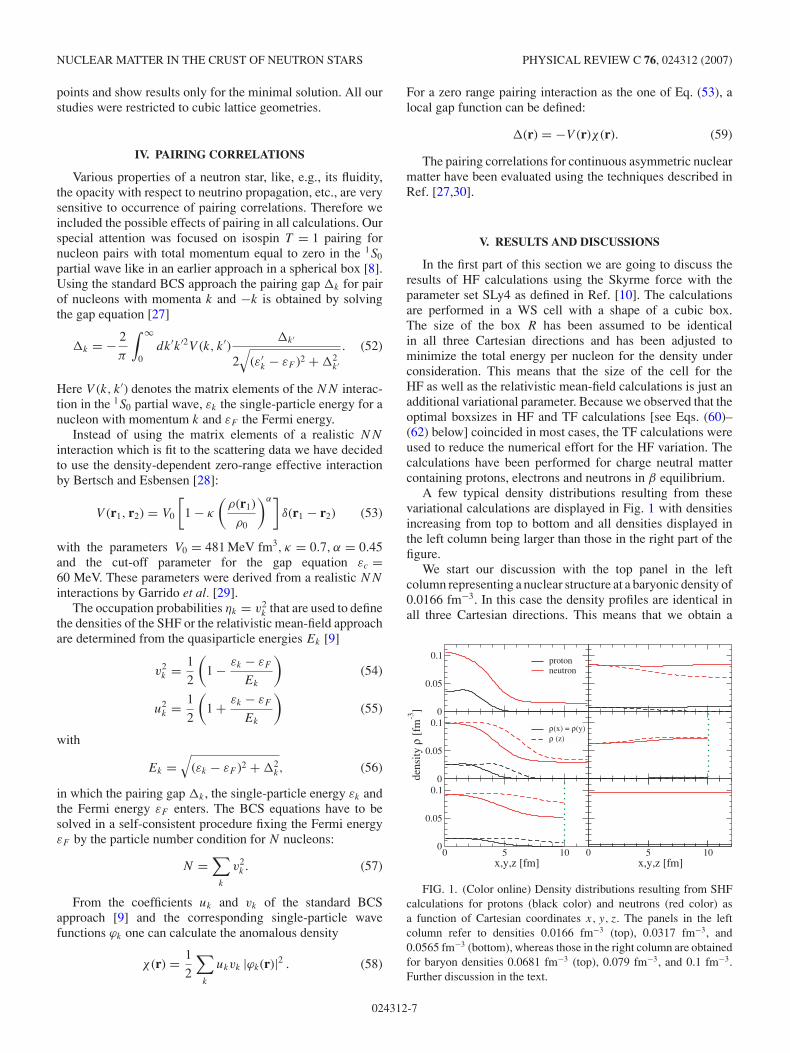
A few typical density distributions resulting from thesevariational calculations are displayed in Fig. 1 with densitiesincreasing from top to bottom and all densities displayed inthe left column being larger than those in the right part of thefigure.

We start our discussion with the top panel in the leftcolumn representing a nuclear structure at a baryonic density of0.0166 fm−3. In this case the density profiles are identical inall three Cartesian directions. This means that we obtain a

0

0.05

0.1 protonneutron

0

0.05

0.1

dens

ity ρ

[fm

-3]

ρ(x) = ρ(y)ρ (z)

0 5 10x,y,z [fm]

0

0.05

0.1

0 5 10x,y,z [fm]

FIG. 1. (Color online) Density distributions resulting from SHFcalculations for protons (black color) and neutrons (red color) asa function of Cartesian coordinates x, y, z. The panels in the leftcolumn refer to densities 0.0166 fm−3 (top), 0.0317 fm−3, and0.0565 fm−3 (bottom), whereas those in the right column are obtainedfor baryon densities 0.0681 fm−3 (top), 0.079 fm−3, and 0.1 fm−3.Further discussion in the text.

024312-7


pro

ton

den

sity

ρp

[fm

−3]

–8–4

04

8 x [fm]

–8–4

04

8 y [fm]

0

0.01

0.02

0.03

0.04

0.05

pro

ton

den

sity

ρp

[fm

−3]

–8–4

04

8 z [fm]

–8–4

04

8 x [fm]

0

0.01

0.02

0.03

0.04

0.05

FIG. 2. Profiles for the proton density distribution forming a rod structure at a density of 0.0625 fm−3.

quasinuclear structure with spherical symmetry in the centerof the WS cell. The proton density drops to zero at a radialdistance of around 4 fm. The neutron density profile dropsaround the same radius from a central density of around0.1 fm−3 to the peripheral value of around 0.01 fm−3. Thismeans that at this density we have obtained a structureof quasinuclear droplets forming a cubic lattice, which isembedded in a sea of neutrons.

The second panel in the left part of Fig. 1 displays thedensity distributions, which have been obtained at a densityof 0.0317 fm−3. In this case we obtain deformed quasinucleardroplets with radii, which are slightly larger in one direction(chosen to be the z direction, dashed curves) than in the othertwo, which means that we find prolate deformation.

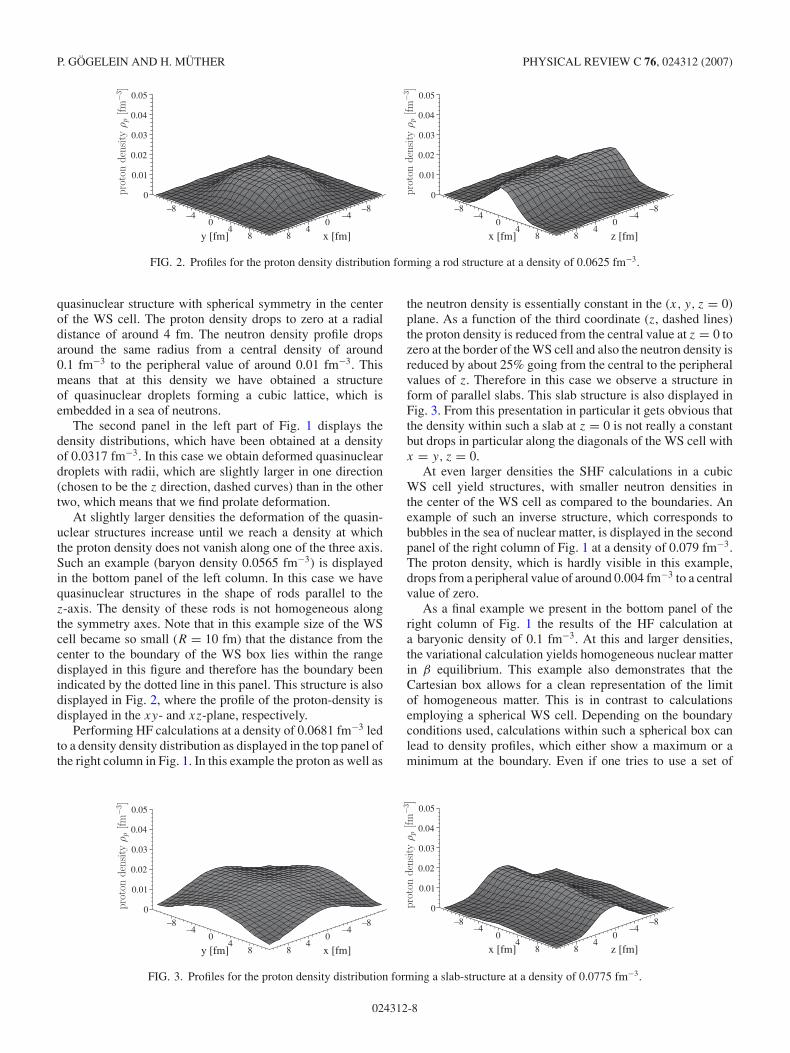
At slightly larger densities the deformation of the quasin-uclear structures increase until we reach a density at whichthe proton density does not vanish along one of the three axis.Such an example (baryon density 0.0565 fm−3) is displayedin the bottom panel of the left column. In this case we havequasinuclear structures in the shape of rods parallel to thez-axis. The density of these rods is not homogeneous alongthe symmetry axes. Note that in this example size of the WScell became so small (R = 10 fm) that the distance from thecenter to the boundary of the WS box lies within the rangedisplayed in this figure and therefore has the boundary beenindicated by the dotted line in this panel. This structure is alsodisplayed in Fig. 2, where the profile of the proton-density isdisplayed in the xy- and xz-plane, respectively.

Performing HF calculations at a density of 0.0681 fm−3 ledto a density density distribution as displayed in the top panel ofthe right column in Fig. 1. In this example the proton as well as

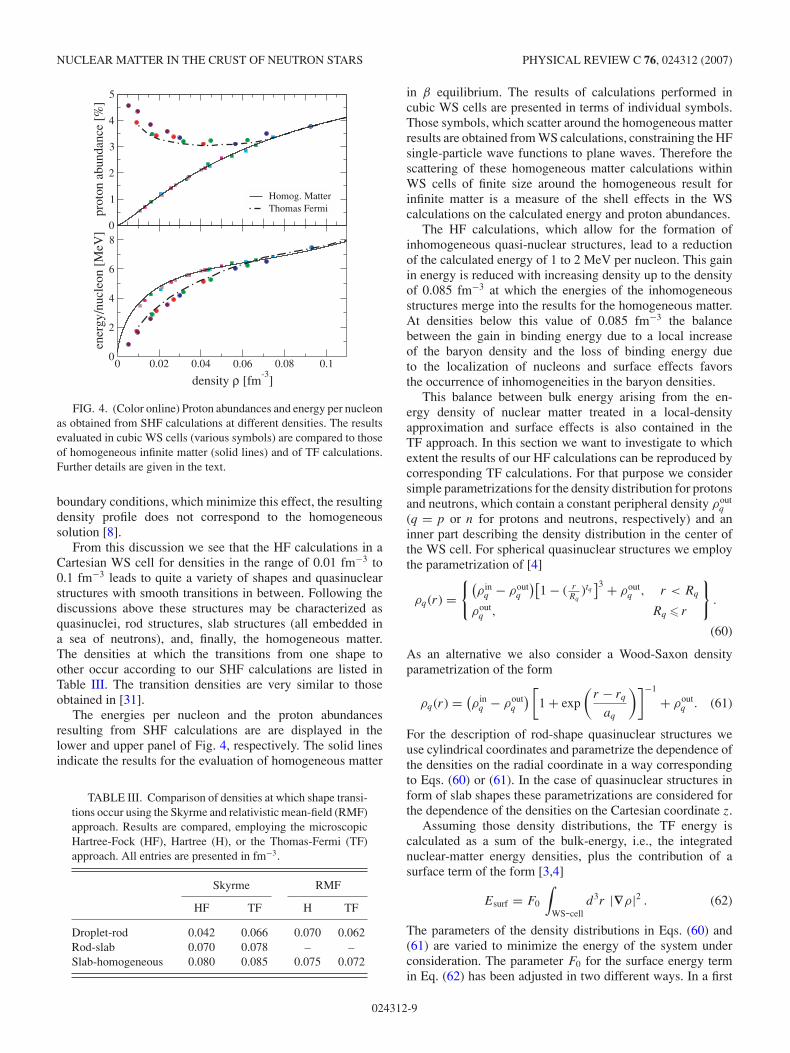
the neutron density is essentially constant in the (x, y, z = 0)plane. As a function of the third coordinate (z, dashed lines)the proton density is reduced from the central value at z = 0 tozero at the border of the WS cell and also the neutron density isreduced by about 25% going from the central to the peripheralvalues of z. Therefore in this case we observe a structure inform of parallel slabs. This slab structure is also displayed inFig. 3. From this presentation in particular it gets obvious thatthe density within such a slab at z = 0 is not really a constantbut drops in particular along the diagonals of the WS cell withx = y, z = 0.

At even larger densities the SHF calculations in a cubicWS cell yield structures, with smaller neutron densities inthe center of the WS cell as compared to the boundaries. Anexample of such an inverse structure, which corresponds tobubbles in the sea of nuclear matter, is displayed in the secondpanel of the right column of Fig. 1 at a density of 0.079 fm−3.The proton density, which is hardly visible in this example,drops from a peripheral value of around 0.004 fm−3 to a centralvalue of zero.

As a final example we present in the bottom panel of theright column of Fig. 1 the results of the HF calculation ata baryonic density of 0.1 fm−3. At this and larger densities,the variational calculation yields homogeneous nuclear matterin β equilibrium. This example also demonstrates that theCartesian box allows for a clean representation of the limitof homogeneous matter. This is in contrast to calculationsemploying a spherical WS cell. Depending on the boundaryconditions used, calculations within such a spherical box canlead to density profiles, which either show a maximum or aminimum at the boundary. Even if one tries to use a set of

pro

ton

den

sity

ρp

[fm

−3]

–8–4

04

8 x [fm]

–8–4

04

8 y [fm]

0

0.01

0.02

0.03

0.04

0.05

pro

ton

den

sity

ρp

[fm

−3]

–8–4

04

8 z [fm]

–8–4

04

8 x [fm]

0

0.01

0.02

0.03

0.04

0.05

FIG. 3. Profiles for the proton density distribution forming a slab-structure at a density of 0.0775 fm−3.

024312-8


0

1

2

3

4

5pr

oton

abu

ndan

ce [

%]

Homog. MatterThomas Fermi

0 0.02 0.04 0.06 0.08 0.1

density ρ [fm-3

]

0

2

4

6

8

ener

gy/n

ucle

on [

MeV

]

FIG. 4. (Color online) Proton abundances and energy per nucleonas obtained from SHF calculations at different densities. The resultsevaluated in cubic WS cells (various symbols) are compared to thoseof homogeneous infinite matter (solid lines) and of TF calculations.Further details are given in the text.

boundary conditions, which minimize this effect, the resultingdensity profile does not correspond to the homogeneoussolution [8].

From this discussion we see that the HF calculations in aCartesian WS cell for densities in the range of 0.01 fm−3 to0.1 fm−3 leads to quite a variety of shapes and quasinuclearstructures with smooth transitions in between. Following thediscussions above these structures may be characterized asquasinuclei, rod structures, slab structures (all embedded ina sea of neutrons), and, finally, the homogeneous matter.The densities at which the transitions from one shape toother occur according to our SHF calculations are listed inTable III. The transition densities are very similar to thoseobtained in [31].

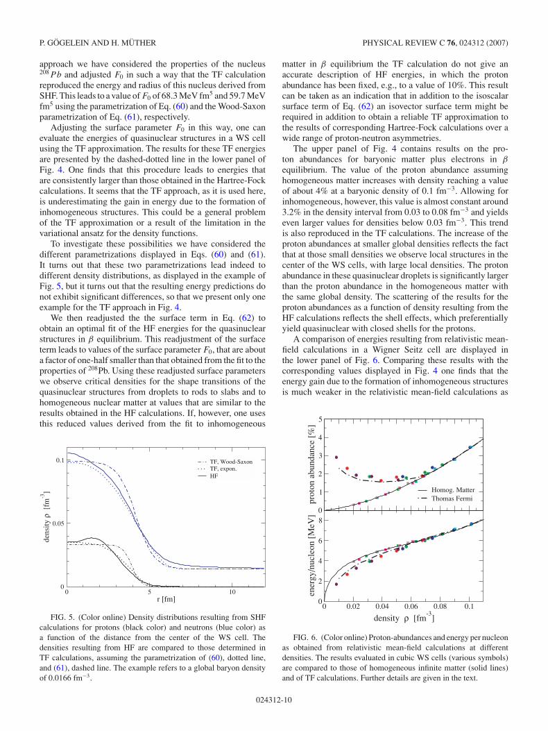
The energies per nucleon and the proton abundancesresulting from SHF calculations are are displayed in thelower and upper panel of Fig. 4, respectively. The solid linesindicate the results for the evaluation of homogeneous matter

TABLE III. Comparison of densities at which shape transi-tions occur using the Skyrme and relativistic mean-field (RMF)approach. Results are compared, employing the microscopicHartree-Fock (HF), Hartree (H), or the Thomas-Fermi (TF)approach. All entries are presented in fm−3.

Skyrme RMF

HF TF H TF

Droplet-rod 0.042 0.066 0.070 0.062Rod-slab 0.070 0.078 – –Slab-homogeneous 0.080 0.085 0.075 0.072

in β equilibrium. The results of calculations performed incubic WS cells are presented in terms of individual symbols.Those symbols, which scatter around the homogeneous matterresults are obtained from WS calculations, constraining the HFsingle-particle wave functions to plane waves. Therefore thescattering of these homogeneous matter calculations withinWS cells of finite size around the homogeneous result forinfinite matter is a measure of the shell effects in the WScalculations on the calculated energy and proton abundances.

The HF calculations, which allow for the formation ofinhomogeneous quasi-nuclear structures, lead to a reductionof the calculated energy of 1 to 2 MeV per nucleon. This gainin energy is reduced with increasing density up to the densityof 0.085 fm−3 at which the energies of the inhomogeneousstructures merge into the results for the homogeneous matter.At densities below this value of 0.085 fm−3 the balancebetween the gain in binding energy due to a local increaseof the baryon density and the loss of binding energy dueto the localization of nucleons and surface effects favorsthe occurrence of inhomogeneities in the baryon densities.

This balance between bulk energy arising from the en-ergy density of nuclear matter treated in a local-densityapproximation and surface effects is also contained in theTF approach. In this section we want to investigate to whichextent the results of our HF calculations can be reproduced bycorresponding TF calculations. For that purpose we considersimple parametrizations for the density distribution for protonsand neutrons, which contain a constant peripheral density ρout

q

(q = p or n for protons and neutrons, respectively) and aninner part describing the density distribution in the center ofthe WS cell. For spherical quasinuclear structures we employthe parametrization of [4]

ρq(r) ={(

ρ inq − ρout

q

)[1 − ( r

Rq)tq

]3 + ρoutq , r < Rq

ρoutq , Rq � r

}.

(60)

As an alternative we also consider a Wood-Saxon densityparametrization of the form

ρq(r) = (ρ in

q − ρoutq

) [1 + exp

(r − rq

aq

)]−1

+ ρoutq . (61)

For the description of rod-shape quasinuclear structures weuse cylindrical coordinates and parametrize the dependence ofthe densities on the radial coordinate in a way correspondingto Eqs. (60) or (61). In the case of quasinuclear structures inform of slab shapes these parametrizations are considered forthe dependence of the densities on the Cartesian coordinate z.

Assuming those density distributions, the TF energy iscalculated as a sum of the bulk-energy, i.e., the integratednuclear-matter energy densities, plus the contribution of asurface term of the form [3,4]

Esurf = F0

∫WS-cell

d3r |∇ρ|2 . (62)

The parameters of the density distributions in Eqs. (60) and(61) are varied to minimize the energy of the system underconsideration. The parameter F0 for the surface energy termin Eq. (62) has been adjusted in two different ways. In a first

024312-9


approach we have considered the properties of the nucleus208Pb and adjusted F0 in such a way that the TF calculationreproduced the energy and radius of this nucleus derived fromSHF. This leads to a value of F0 of 68.3 MeV fm5 and 59.7 MeVfm5 using the parametrization of Eq. (60) and the Wood-Saxonparametrization of Eq. (61), respectively.

Adjusting the surface parameter F0 in this way, one canevaluate the energies of quasinuclear structures in a WS cellusing the TF approximation. The results for these TF energiesare presented by the dashed-dotted line in the lower panel ofFig. 4. One finds that this procedure leads to energies thatare consistently larger than those obtained in the Hartree-Fockcalculations. It seems that the TF approach, as it is used here,is underestimating the gain in energy due to the formation ofinhomogeneous structures. This could be a general problemof the TF approximation or a result of the limitation in thevariational ansatz for the density functions.

To investigate these possibilities we have considered thedifferent parametrizations displayed in Eqs. (60) and (61).It turns out that these two parametrizations lead indeed todifferent density distributions, as displayed in the example ofFig. 5, but it turns out that the resulting energy predictions donot exhibit significant differences, so that we present only oneexample for the TF approach in Fig. 4.

We then readjusted the the surface term in Eq. (62) toobtain an optimal fit of the HF energies for the quasinuclearstructures in β equilibrium. This readjustment of the surfaceterm leads to values of the surface parameter F0, that are abouta factor of one-half smaller than that obtained from the fit to theproperties of 208Pb. Using these readjusted surface parameterswe observe critical densities for the shape transitions of thequasinuclear structures from droplets to rods to slabs and tohomogeneous nuclear matter at values that are similar to theresults obtained in the HF calculations. If, however, one usesthis reduced values derived from the fit to inhomogeneous

0 5 10r [fm]

0

0.05

0.1

dens

ity ρ

[fm

-3]

TF, Wood-SaxonTF, expon.HF

FIG. 5. (Color online) Density distributions resulting from SHFcalculations for protons (black color) and neutrons (blue color) asa function of the distance from the center of the WS cell. Thedensities resulting from HF are compared to those determined inTF calculations, assuming the parametrization of (60), dotted line,and (61), dashed line. The example refers to a global baryon densityof 0.0166 fm−3.

matter in β equilibrium the TF calculation do not give anaccurate description of HF energies, in which the protonabundance has been fixed, e.g., to a value of 10%. This resultcan be taken as an indication that in addition to the isoscalarsurface term of Eq. (62) an isovector surface term might berequired in addition to obtain a reliable TF approximation tothe results of corresponding Hartree-Fock calculations over awide range of proton-neutron asymmetries.

The upper panel of Fig. 4 contains results on the pro-ton abundances for baryonic matter plus electrons in β

equilibrium. The value of the proton abundance assuminghomogeneous matter increases with density reaching a valueof about 4% at a baryonic density of 0.1 fm−3. Allowing forinhomogeneous, however, this value is almost constant around3.2% in the density interval from 0.03 to 0.08 fm−3 and yieldseven larger values for densities below 0.03 fm−3. This trendis also reproduced in the TF calculations. The increase of theproton abundances at smaller global densities reflects the factthat at those small densities we observe local structures in thecenter of the WS cells, with large local densities. The protonabundance in these quasinuclear droplets is significantly largerthan the proton abundance in the homogeneous matter withthe same global density. The scattering of the results for theproton abundances as a function of density resulting from theHF calculations reflects the shell effects, which preferentiallyyield quasinuclear with closed shells for the protons.

A comparison of energies resulting from relativistic mean-field calculations in a Wigner Seitz cell are displayed inthe lower panel of Fig. 6. Comparing these results with thecorresponding values displayed in Fig. 4 one finds that theenergy gain due to the formation of inhomogeneous structuresis much weaker in the relativistic mean-field calculations as

0

1

2

3

4

5

prot

on a

bund

ance

[%

]

Homog. MatterThomas Fermi

0 0.02 0.04 0.06 0.08 0.1

density ρ [fm-3]

0

2

4

6

8

ener

gy/n

ucle

on [

MeV

]

FIG. 6. (Color online) Proton-abundances and energy per nucleonas obtained from relativistic mean-field calculations at differentdensities. The results evaluated in cubic WS cells (various symbols)are compared to those of homogeneous infinite matter (solid lines)and of TF calculations. Further details are given in the text.

024312-10


compared to the Skyrme model. This is also reflected in thecorresponding TF calculations. Note that also in this case wehave adjusted the constant F0 of the surface term in Eq. (62)to reproduce the bulk properties of 208Pb as predicted by therelativistic mean-field calculations. This leads to value for F0

of 87.4 MeV fm5 and 80.3 MeV fm5 using the parametrizationof Eq. (60) and the Wood-Saxon parametrization of Eq. (61),respectively. Both values are significantly larger than thevalues required for F0 in the case of the Skyrme model usedabove.

The different interplay between volume, surface, symmetry,and Coulomb effects in the relativistic mean-field model ascompared to the Skyrme model also leads to smaller valuesfor the proton abundance in the region of nuclear densities, inwhich inhomogeneous structures emerge. The values aroundρ = 0.02 fm−3, displayed in the upper panel of Fig. 6, areabout 40% smaller than the corresponding values obtained inthe Skyrme model (see Fig. 4). The differences in the balancebetween volume and surface contributions to the energy alsolead to different quasinuclear structures in the nuclear modelsunder consideration. It is worth mentioning that within therelativistic mean-field mode we do not find any formation ofslablike structures. Therefore the Table III contains for thiscase only transition densities for droplet to rod structures andthe formation of a homogeneous structure.

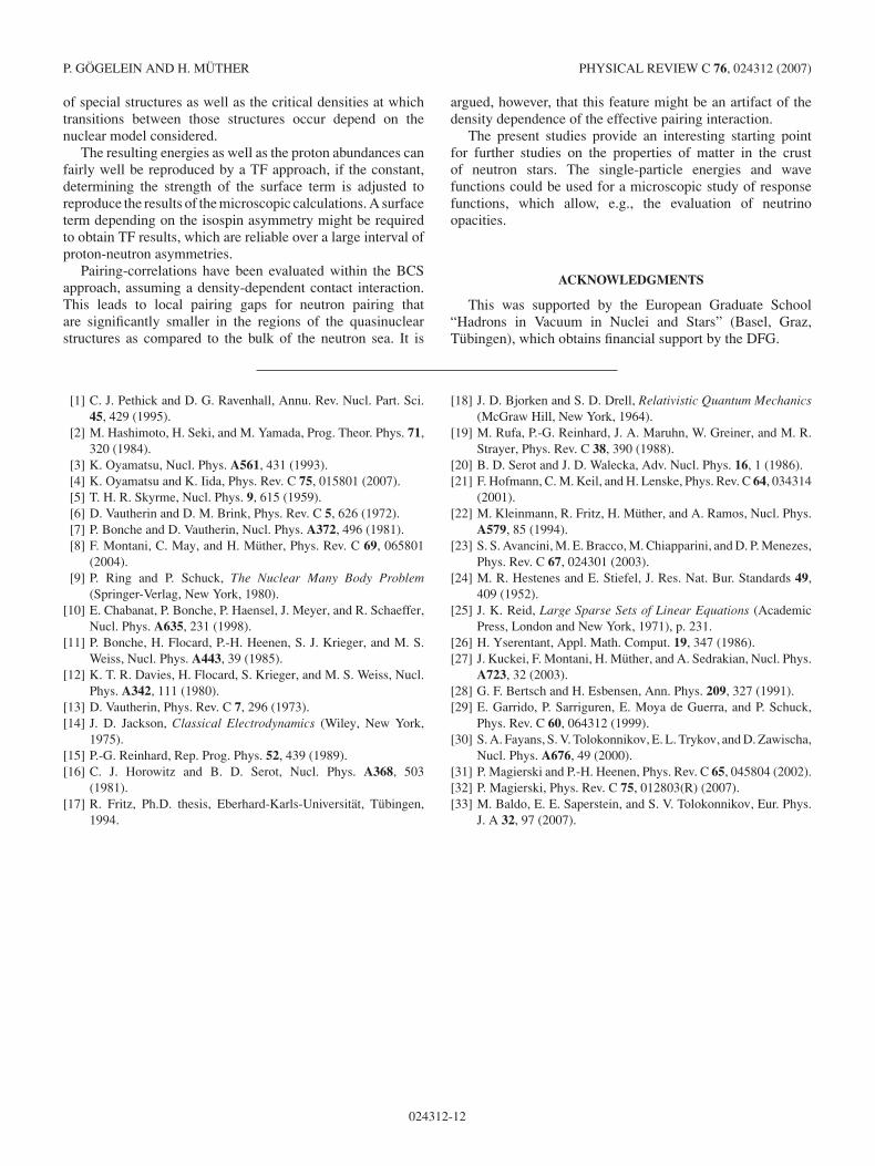
The density profiles obtained from these two approachesalso yield different results. As an example we present in Fig. 7the density profiles at ρ = 0.032 fm−3, a density at which boththe relativistic as well as the Skyrme model yield a dropletstructure. Note, that in the case of the Skyrme calculationwe obtain a WS cell with a length of 26.4 fm that leadsto a borderline as indicated by the dotted line, whereas thecorresponding borderline for the RMF calculation is identicalto the frame of the figure.

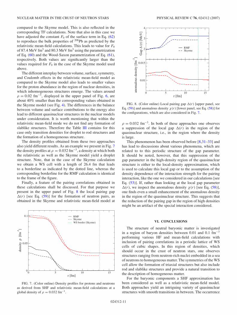
Finally, a feature of the pairing correlations obtained inthese calculations shall be discussed. For that purpose wepresent in the upper panel of Fig. 8 the local pairing gap�(r) [see Eq. (59)] for the formation of neutron pairs, asobtained in the Skyrme and relativistic mean-field model at

0 5 10 15r [fm]

0

0.05

0.1

dens

ity ρ

[fm

-3]

RMFSkyrmeWS border (Skyrme)

FIG. 7. (Color online) Density profiles for protons and neutronsas derived from SHF and relativistic mean-field calculations at aglobal density of ρ = 0.032 fm−3.

2

3

4

Gap

∆ (

r) [

MeV

]

RMFSkyrme

0 5 10 15r [fm]

0.01

0.015

anom

alou

s de

nsity

[fm

-3]

FIG. 8. (Color online) Local pairing gap �(r) [upper panel, seeEq. (59)] and anomalous density χ (r) [lower panel, see Eq. (58)] forthe configurations, which are also considered in Fig. 7.

ρ = 0.032 fm−3. In both of these approaches one observesa suppression of the local gap �(r) in the region of thequasinuclear structure, i.e., in the region where the densityis large.

This phenomenon has been observed before [8,31–33] andhas lead to discussions about various phenomena, which arerelated to to this periodic structure of the gap parameter.It should be noted, however, that this suppression of thegap parameter in the high-density region of the quasinuclearstructure is either to the local-density approximation, whichis used to calculate this local gap or to the assumption of thedensity dependence of the interaction strength for the pairinginteraction, like the one we considered in our calculations [seeEq. (53)]. If, rather than looking at the local gap parameter�(r), we inspect the anomalous density χ (r) [see Eq. (58)],one finds even a small enhancement of the anomalous densityin the region of the quasinuclear structure. This suggests thatthe reduction of the pairing gap in the region of high densitiesmight be an artifact of the special interaction considered.

VI. CONCLUSIONS

The structure of neutral baryonic matter is investigatedin a region of baryon densities between 0.01 and 0.1 fm−3

performing various HF and mean-field calculations withinclusion of pairing correlations in a periodic lattice of WScells of cubic shapes. In this region of densities, whichshould occur in the crust of neutron stars, one observesstructures ranging from neutron-rich nuclei embedded in a seaof neutrons to homogeneous matter. The symmetries of the WScell allow the formation of triaxial structures but also includerod and slablike structures and provide a natural transition tothe description of homogeneous matter.

For the baryonic components a SHF approximation hasbeen considered as well as a relativistic mean-field model.Both approaches yield an intriguing variety of quasinuclearstructures with smooth transitions in between. The occurrence

024312-11


of special structures as well as the critical densities at whichtransitions between those structures occur depend on thenuclear model considered.

The resulting energies as well as the proton abundances canfairly well be reproduced by a TF approach, if the constant,determining the strength of the surface term is adjusted toreproduce the results of the microscopic calculations. A surfaceterm depending on the isospin asymmetry might be requiredto obtain TF results, which are reliable over a large interval ofproton-neutron asymmetries.

Pairing-correlations have been evaluated within the BCSapproach, assuming a density-dependent contact interaction.This leads to local pairing gaps for neutron pairing thatare significantly smaller in the regions of the quasinuclearstructures as compared to the bulk of the neutron sea. It is

argued, however, that this feature might be an artifact of thedensity dependence of the effective pairing interaction.

The present studies provide an interesting starting pointfor further studies on the properties of matter in the crustof neutron stars. The single-particle energies and wavefunctions could be used for a microscopic study of responsefunctions, which allow, e.g., the evaluation of neutrinoopacities.

ACKNOWLEDGMENTS

This was supported by the European Graduate School“Hadrons in Vacuum in Nuclei and Stars” (Basel, Graz,Tubingen), which obtains financial support by the DFG.

[1] C. J. Pethick and D. G. Ravenhall, Annu. Rev. Nucl. Part. Sci.45, 429 (1995).

[2] M. Hashimoto, H. Seki, and M. Yamada, Prog. Theor. Phys. 71,320 (1984).

[3] K. Oyamatsu, Nucl. Phys. A561, 431 (1993).[4] K. Oyamatsu and K. Iida, Phys. Rev. C 75, 015801 (2007).[5] T. H. R. Skyrme, Nucl. Phys. 9, 615 (1959).[6] D. Vautherin and D. M. Brink, Phys. Rev. C 5, 626 (1972).[7] P. Bonche and D. Vautherin, Nucl. Phys. A372, 496 (1981).[8] F. Montani, C. May, and H. Muther, Phys. Rev. C 69, 065801

(2004).[9] P. Ring and P. Schuck, The Nuclear Many Body Problem

(Springer-Verlag, New York, 1980).[10] E. Chabanat, P. Bonche, P. Haensel, J. Meyer, and R. Schaeffer,

Nucl. Phys. A635, 231 (1998).[11] P. Bonche, H. Flocard, P.-H. Heenen, S. J. Krieger, and M. S.

Weiss, Nucl. Phys. A443, 39 (1985).[12] K. T. R. Davies, H. Flocard, S. Krieger, and M. S. Weiss, Nucl.

Phys. A342, 111 (1980).[13] D. Vautherin, Phys. Rev. C 7, 296 (1973).[14] J. D. Jackson, Classical Electrodynamics (Wiley, New York,

1975).[15] P.-G. Reinhard, Rep. Prog. Phys. 52, 439 (1989).[16] C. J. Horowitz and B. D. Serot, Nucl. Phys. A368, 503

(1981).[17] R. Fritz, Ph.D. thesis, Eberhard-Karls-Universitat, Tubingen,

1994.

[18] J. D. Bjorken and S. D. Drell, Relativistic Quantum Mechanics(McGraw Hill, New York, 1964).

[19] M. Rufa, P.-G. Reinhard, J. A. Maruhn, W. Greiner, and M. R.Strayer, Phys. Rev. C 38, 390 (1988).

[20] B. D. Serot and J. D. Walecka, Adv. Nucl. Phys. 16, 1 (1986).[21] F. Hofmann, C. M. Keil, and H. Lenske, Phys. Rev. C 64, 034314

(2001).[22] M. Kleinmann, R. Fritz, H. Muther, and A. Ramos, Nucl. Phys.

A579, 85 (1994).[23] S. S. Avancini, M. E. Bracco, M. Chiapparini, and D. P. Menezes,

Phys. Rev. C 67, 024301 (2003).[24] M. R. Hestenes and E. Stiefel, J. Res. Nat. Bur. Standards 49,

409 (1952).[25] J. K. Reid, Large Sparse Sets of Linear Equations (Academic

Press, London and New York, 1971), p. 231.[26] H. Yserentant, Appl. Math. Comput. 19, 347 (1986).[27] J. Kuckei, F. Montani, H. Muther, and A. Sedrakian, Nucl. Phys.

A723, 32 (2003).[28] G. F. Bertsch and H. Esbensen, Ann. Phys. 209, 327 (1991).[29] E. Garrido, P. Sarriguren, E. Moya de Guerra, and P. Schuck,

Phys. Rev. C 60, 064312 (1999).[30] S. A. Fayans, S. V. Tolokonnikov, E. L. Trykov, and D. Zawischa,

Nucl. Phys. A676, 49 (2000).[31] P. Magierski and P.-H. Heenen, Phys. Rev. C 65, 045804 (2002).[32] P. Magierski, Phys. Rev. C 75, 012803(R) (2007).[33] M. Baldo, E. E. Saperstein, and S. V. Tolokonnikov, Eur. Phys.

J. A 32, 97 (2007).

024312-12

Documents

Nuclear matter in the crust of neutron stars