Embed Size (px)
Citation preview
Nuclear Structure studies using Advanced-GAmma-Tracking techniques
Caterina Michelagnoli [email protected]
École Joliot-Curie 2015
``Instrumentation, detection and simulation in modern nuclear physics’’
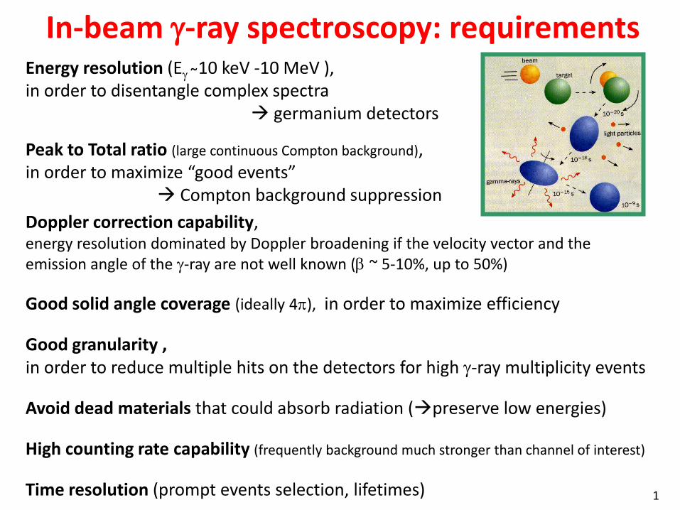
In-beam g-ray spectroscopy: requirements Energy resolution (Eg ̴10 keV -10 MeV ), in order to disentangle complex spectra germanium detectors
Peak to Total ratio (large continuous Compton background), in order to maximize “good events” Compton background suppression Doppler correction capability, energy resolution dominated by Doppler broadening if the velocity vector and the emission angle of the g-ray are not well known (b ~ 5-10%, up to 50%)
Good solid angle coverage (ideally 4p), in order to maximize efficiency
Good granularity , in order to reduce multiple hits on the detectors for high g-ray multiplicity events
Avoid dead materials that could absorb radiation (preserve low energies)
High counting rate capability (frequently background much stronger than channel of interest)
Time resolution (prompt events selection, lifetimes) 1

Position-sensitive operation mode and g-ray tracking
highly segmented HPGe detectors
Event by event: how many gammas,
for each gamma: energy, first interaction point, path
digital electronics to record sampled
waveforms
Pulse Shape Analysis of the recorded waves
Identified interaction points
(hits)
(x,y,z,E,t)i
reconstruction of g-rays from the hits
(tracking)
2

(be aware … personal selection of topics!)
PART 2 (September 29th 2015) Pulse Shape Analysis (PSA) 1. Signal bases calculation 2. Signal decomposition Some results from Ge position sensitive mode operation and γ-ray tracking
The AGATA array of segmented HPGe detectors 1. Implementation of Pulse Shape Analysis and Tracking concepts 2. The AGATA detectors and preamplifiers 3. The structure of electronics and data acquisition 4. Digital signal processing (at high counting rate) 5. (AGATA data processing)
AGATA+VAMOS (magnetic spectrometer) at GANIL
Outline
3
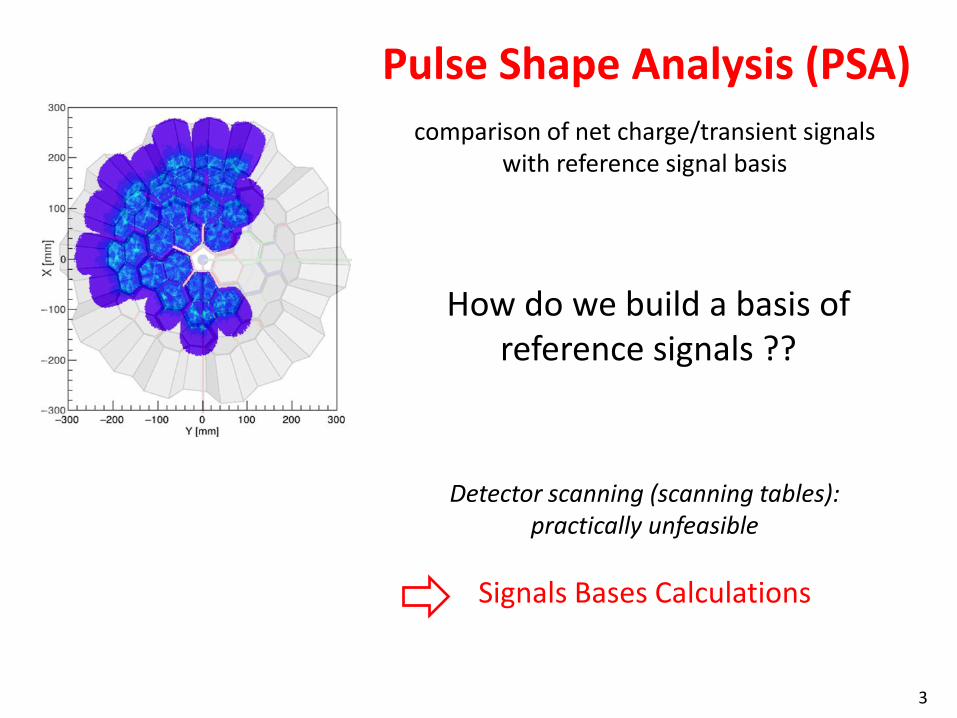
Pulse Shape Analysis (PSA)
comparison of net charge/transient signals with reference signal basis
How do we build a basis of reference signals ??
Detector scanning (scanning tables): practically unfeasible
Signals Bases Calculations
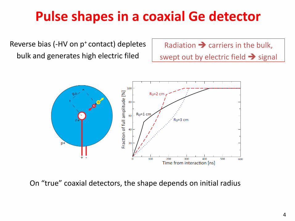
Pulse shapes in a coaxial Ge detector
4
Radiation carriers in the bulk,
swept out by electric field signal
Reverse bias (-HV on p+ contact) depletes
bulk and generates high electric filed
On “true” coaxial detectors, the shape depends on initial radius

Signal Formation • Signal : motion of charge carriers (e/h) inside the detector volume;
ve/h=μe/hE (μe/h = electron/hole mobility)
• Calculation of charge induced in an electrode due to motion of charge carriers in a detector: Ramo Theorem and concept of weighting potential
i(t) = q v EW EW=weighting field
Q = q ΔφW φW=weighting potential
φW =φW ( x ) solution of the Laplace equation (for given detector geometry)
with voltage of the electrode for which induced charge is calculated = 1 and other electrodes at zero
5
i i
iiiiQVQV
''The Ramo theorem is based on the Green’s reciprocity theorem
relation between two systems consisting of a distribution of charges and electrodes
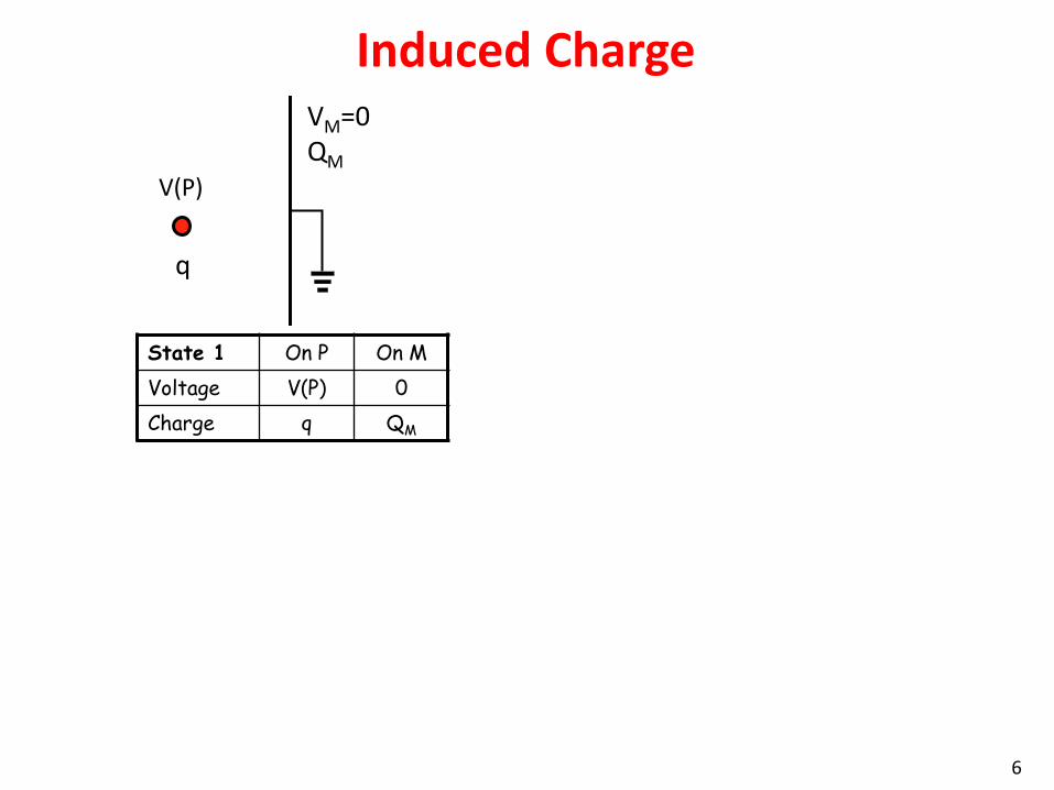
State 1 On P On M
Voltage V(P) 0
Charge q QM
q
V(P)
VM=0 QM
Induced Charge
6
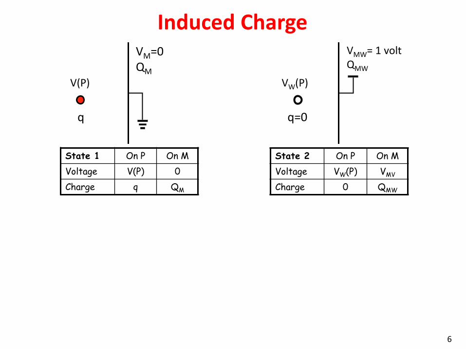
State 1 On P On M
Voltage V(P) 0
Charge q QM
State 2 On P On M
Voltage VW(P) VMV
Charge 0 QMW
q
V(P)
VM=0 QM
Induced Charge VMW= 1 volt QMW
q=0
VW(P)
6
State 1 On P On M
Voltage V(P) 0
Charge q QM
State 2 On P On M
Voltage VW(P) VMV
Charge 0 QMW
q
V(P)
VM=0 QM
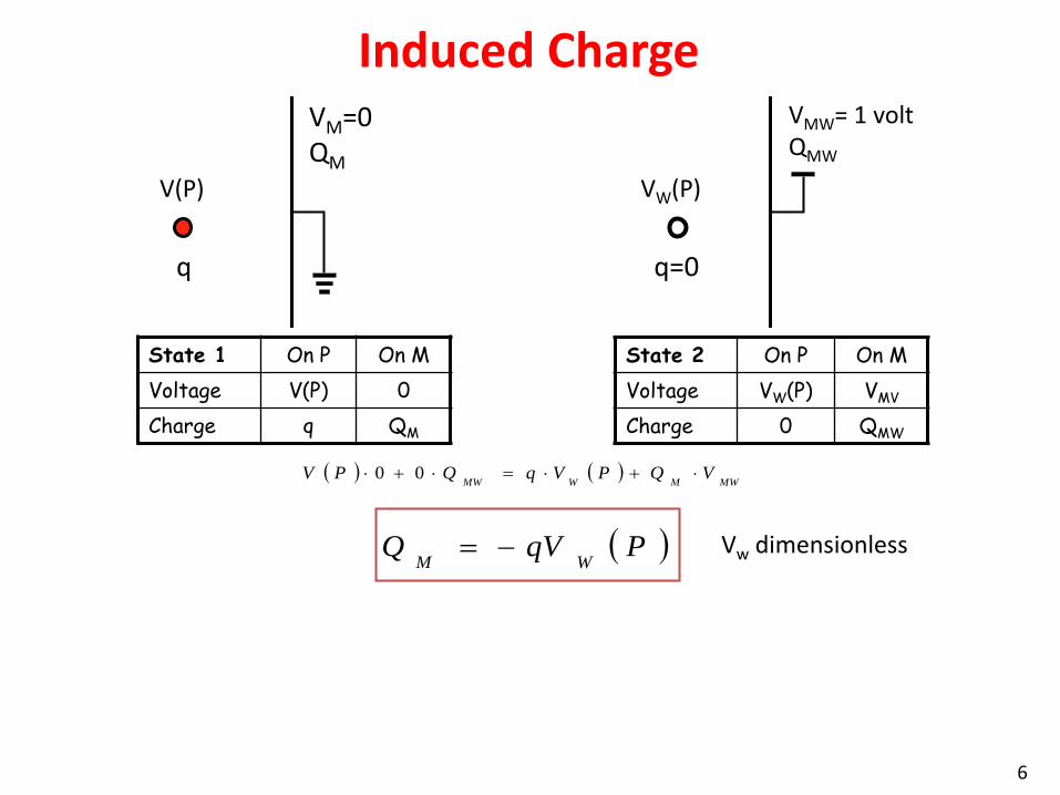
MWMWMW
VQPVqQPV 00
Induced Charge
PqVQWM
VMW= 1 volt QMW
q=0
VW(P)
Vw dimensionless
6
State 1 On P On M
Voltage V(P) 0
Charge q QM
State 2 On P On M
Voltage VW(P) VMV
Charge 0 QMW
q
V(P)
VM=0 QM
MWMWMW
VQPVqQPV 00
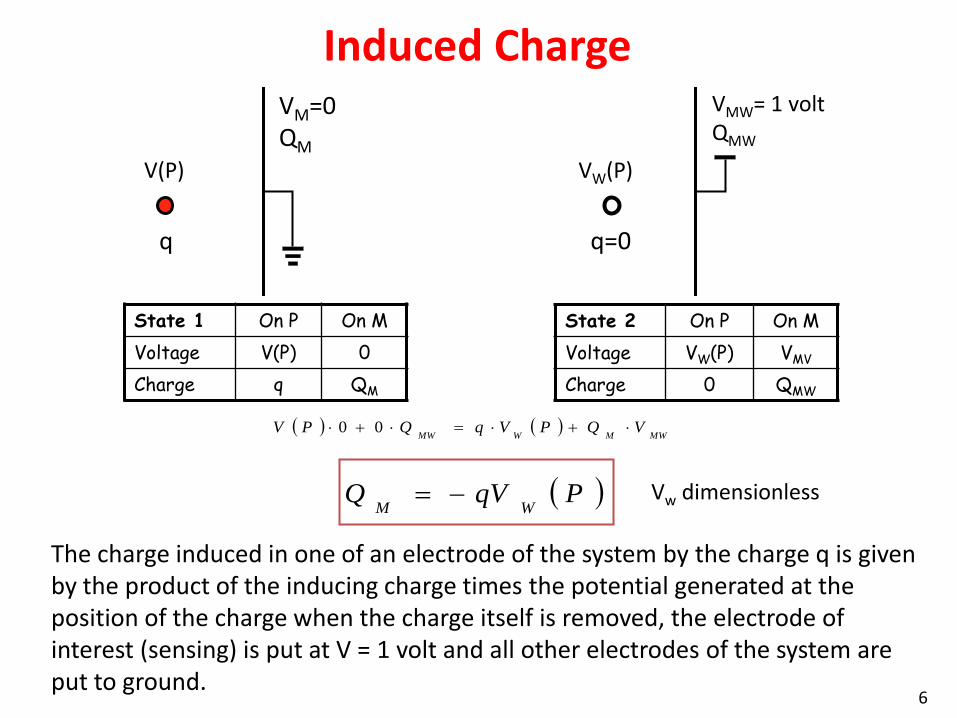
Induced Charge
The charge induced in one of an electrode of the system by the charge q is given by the product of the inducing charge times the potential generated at the position of the charge when the charge itself is removed, the electrode of interest (sensing) is put at V = 1 volt and all other electrodes of the system are put to ground.
PqVQWM
VMW= 1 volt QMW
q=0
VW(P)
Vw dimensionless
6

1 V 0.5 V 0 V
4000 V 2000 V 0 V
Real potential Weighting potential
7
Weighting potential
electrostatic coupling between the moving charge and the sensing electrode
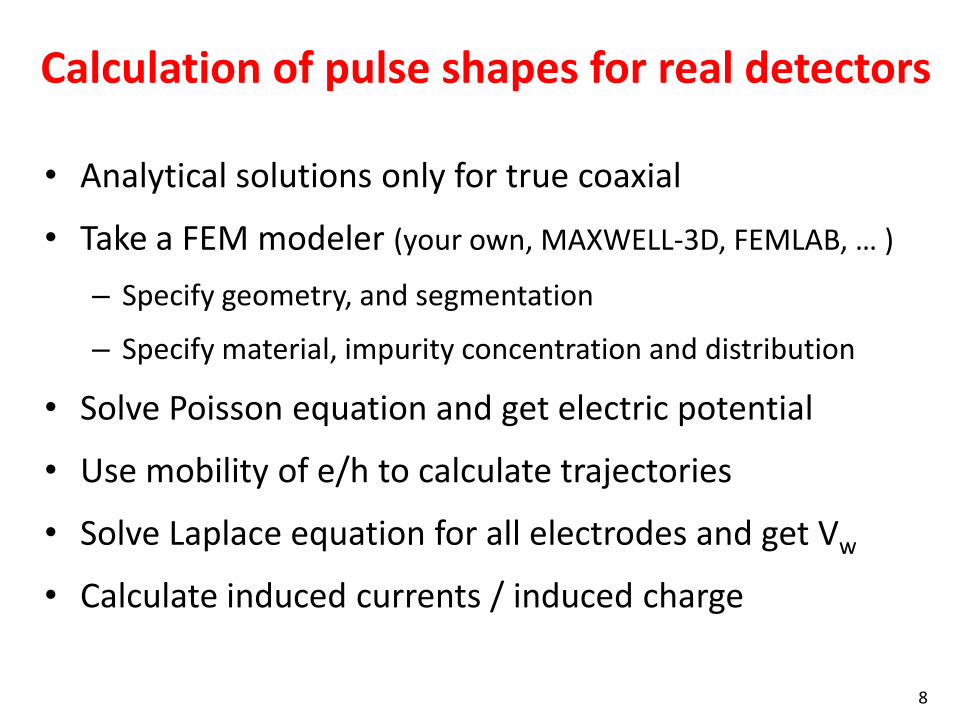
• Analytical solutions only for true coaxial
• Take a FEM modeler (your own, MAXWELL-3D, FEMLAB, … )
– Specify geometry, and segmentation
– Specify material, impurity concentration and distribution
• Solve Poisson equation and get electric potential
• Use mobility of e/h to calculate trajectories
• Solve Laplace equation for all electrodes and get Vw
• Calculate induced currents / induced charge
8
Calculation of pulse shapes for real detectors
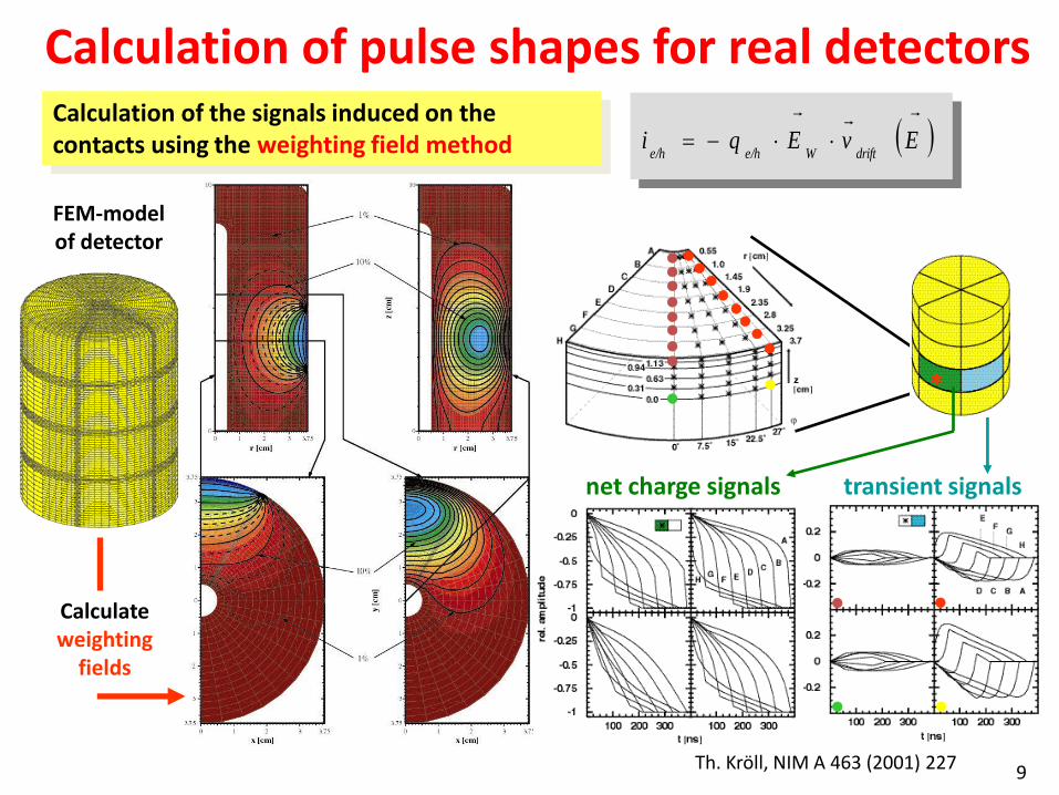
Calculation of pulse shapes for real detectors
FEM-model of detector
Calculate weighting
fields
EvEqidriftWe/he/h
*
Calculation of the signals induced on the contacts using the weighting field method
transient signals
net charge signals
Th. Kröll, NIM A 463 (2001) 227 9
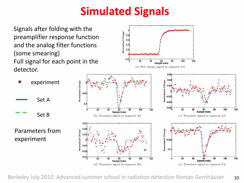
Simulated Signals
Signals after folding with the preamplifier response function and the analog filter functions (some smearing) Full signal for each point in the detector.
experiment
Set A
Set B
Parameters from experiment
Berkeley July 2010 Advanced summer school in radiation detection Roman Gernhäuser 10

Signal Decomposition or Pulse Shape Analysis (PSA)
• Sampling every 10 ns, ̴100 samples per involved segment
• Each base-point has 1 segment with net charge and 8-11 neighbours with transient signals
• With a grid of 1 mm a typical crystal has ~ 400000 base points (up to possible symmetries)
Expand measured signals in terms of base signals and determine expansion coefficients
N
i
base
ii
exp
SAS
1
That’s too much for a direct decomposition !!!
11
Grid Search Algorithm
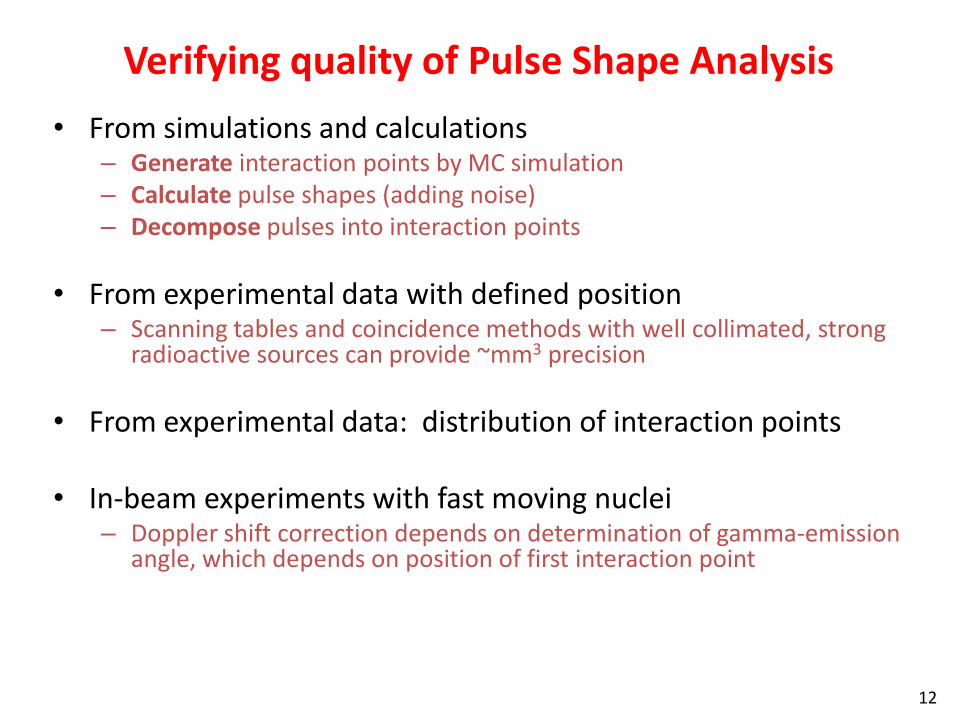
Verifying quality of Pulse Shape Analysis
• From simulations and calculations – Generate interaction points by MC simulation – Calculate pulse shapes (adding noise) – Decompose pulses into interaction points
• From experimental data with defined position – Scanning tables and coincidence methods with well collimated, strong
radioactive sources can provide ~mm3 precision
• From experimental data: distribution of interaction points • In-beam experiments with fast moving nuclei
– Doppler shift correction depends on determination of gamma-emission angle, which depends on position of first interaction point
12
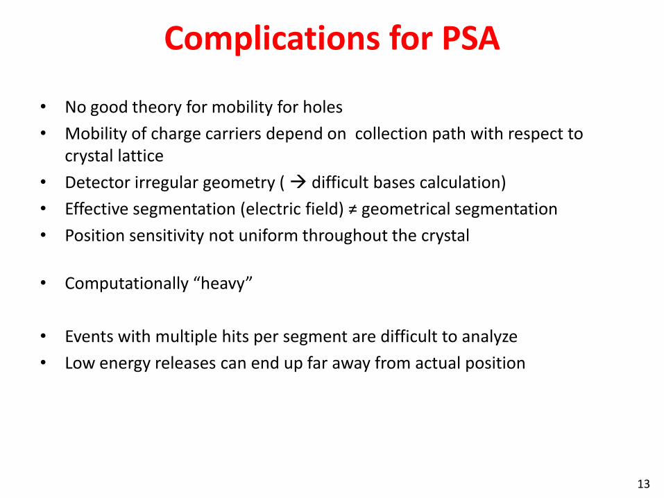
Complications for PSA
• No good theory for mobility for holes
• Mobility of charge carriers depend on collection path with respect to crystal lattice
• Detector irregular geometry ( difficult bases calculation)
• Effective segmentation (electric field) ≠ geometrical segmentation
• Position sensitivity not uniform throughout the crystal
• Computationally “heavy”
• Events with multiple hits per segment are difficult to analyze
• Low energy releases can end up far away from actual position
13
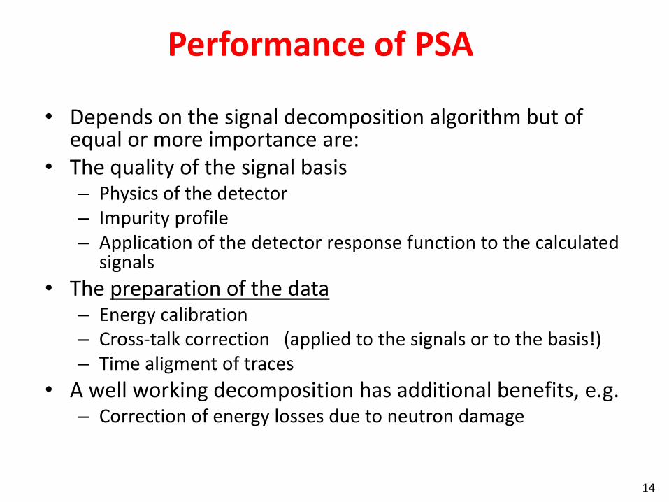
Performance of PSA
• Depends on the signal decomposition algorithm but of equal or more importance are:
• The quality of the signal basis – Physics of the detector – Impurity profile – Application of the detector response function to the calculated
signals
• The preparation of the data – Energy calibration – Cross-talk correction (applied to the signals or to the basis!) – Time aligment of traces
• A well working decomposition has additional benefits, e.g. – Correction of energy losses due to neutron damage
14
Some benefits from position resolution and g-ray tracking

Doppler broadening: towards the intrinsic resolution in-beam
10
keV
v/c ~ 50%
136Xe (137 MeV/u) + 197Au
AGATA @ GSI-FRS commissioning run
Doppler correction using center of crystals FWHM ~20 keV
Doppler correction using center of hit segments FWHM = 7 keV
Doppler correction using PSA (AGS) and tracking FWHM = 3.5 keV (3.2 keV if only single hits)
Eg (keV)
v/c ~ 8% E(2+) = 846.8 keV
1 triple cluster + PPAC at Legnaro !!
220 MeV 56Fe 197Au
2+ 0+ 98Zr populated by fission GANIL
AGATA+VAMOS
EXOGAM+VAMOS
Gain of a factor of 2 !!
15
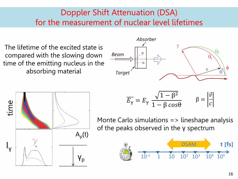
Doppler Shift Attenuation (DSA) for the measurement of nuclear level lifetimes
Iγ
Ap(t)
γp
The lifetime of the excited state is compared with the slowing down
time of the emitting nucleus in the absorbing material
Monte Carlo simulations => lineshape analysis of the peaks observed in the γ spectrum
10-1 1 10 102 103 104
DSAM t [fs]
105
16
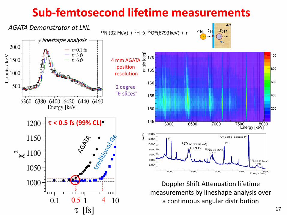
Sub-femtosecond lifetime measurements AGATA Demonstrator at LNL
g lineshape analysis
14N (32 MeV) + 2H 15O*(6793 keV) + n
t < 0.5 fs (99% CL)
4 mm AGATA position
resolution
2 degree “θ slices”
Doppler Shift Attenuation lifetime measurements by lineshape analysis over
a continuous angular distribution 17
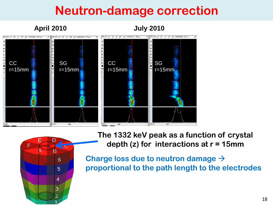
The 1332 keV peak as a function of crystal
depth (z) for interactions at r = 15mm
CC
r=15mm
SG
r=15mm
April 2010
CC
r=15mm
SG
r=15mm
July 2010
Neutron-damage correction
Charge loss due to neutron damage
proportional to the path length to the electrodes
18
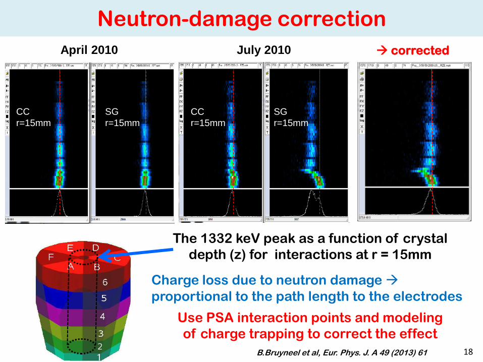
The 1332 keV peak as a function of crystal
depth (z) for interactions at r = 15mm
corrected
CC
r=15mm
SG
r=15mm
April 2010
CC
r=15mm
SG
r=15mm
July 2010
Neutron-damage correction
Charge loss due to neutron damage
proportional to the path length to the electrodes
Use PSA interaction points and modeling
of charge trapping to correct the effect
B.Bruyneel et al, Eur. Phys. J. A 49 (2013) 61 18
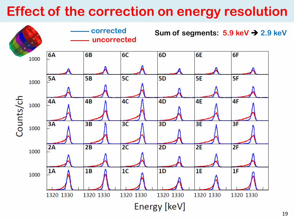
uncorrected
corrected
Effect of the correction on energy resolution
Sum of segments: 5.9 keV 2.9 keV
19
The Advanced-GAmma-Trackig-Array AGATA
S. Akkoyun et al. NIM A 668 (2012) 26
20
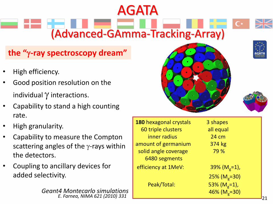
AGATA
(Advanced-GAmma-Tracking-Array)
180 hexagonal crystals 3 shapes 60 triple clusters all equal inner radius 24 cm amount of germanium 374 kg solid angle coverage 79 % 6480 segments
efficiency at 1MeV: 39% (Mg=1),
25% (Mg=30)
Peak/Total: 53% (Mg=1), 46% (Mg=30)
• High efficiency.
• Good position resolution on the
individual g interactions.
• Capability to stand a high counting rate.
• High granularity.
• Capability to measure the Compton scattering angles of the g-rays within the detectors.
• Coupling to ancillary devices for added selectivity.
the “g-ray spectroscopy dream”
21 E. Farnea, NIMA 621 (2010) 331 Geant4 Montecarlo simulations
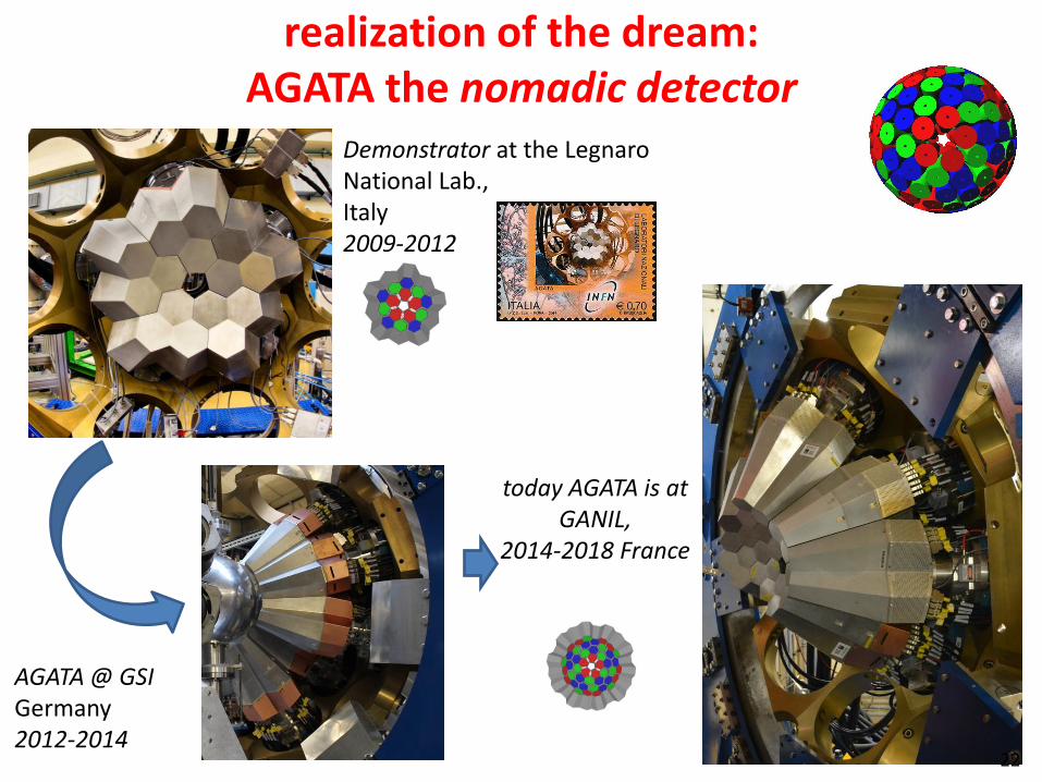
realization of the dream: AGATA the nomadic detector
Demonstrator at the Legnaro National Lab., Italy 2009-2012
AGATA @ GSI Germany 2012-2014
today AGATA is at GANIL,
2014-2018 France
22

AGATA Crystals
Volume ~370 cc Weight ~2 kg (the 3 shapes are volume-equalized to 1%)
80 mm
90
mm
6x6 segmented cathode 23
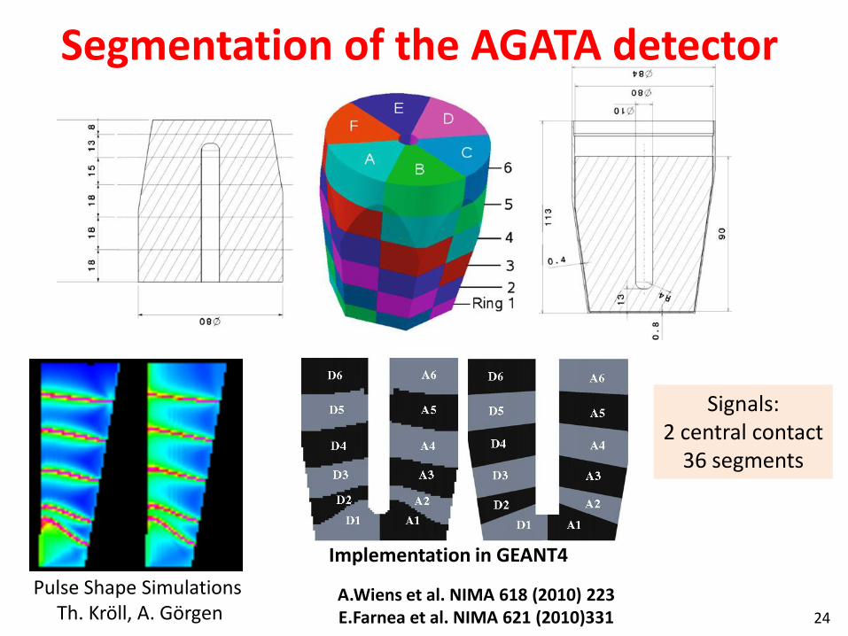
Pulse Shape Simulations Th. Kröll, A. Görgen
A.Wiens et al. NIMA 618 (2010) 223 E.Farnea et al. NIMA 621 (2010)331
Segmentation of the AGATA detector
Implementation in GEANT4
Signals: 2 central contact
36 segments
24

Asymmetric AGATA Triple Cryostat
Challenges: - mechanical precision - heat development, LN2 consumption - microphonics - noise, high frequencies
- integration of 111 high resolution spectroscopy channels - cold FET technology for all signals
Courtesy P. Reiter
A. Wiens et al. NIM A 618 (2010) 223–233 D. Lersch et al. NIM A 640(2011) 133-138
25
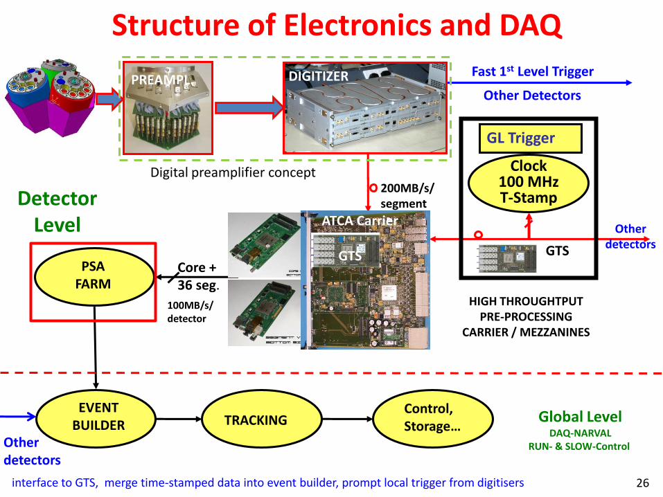
Structure of Electronics and DAQ
TRACKING Control, Storage…
EVENT BUILDER
PSA FARM
Core + 36 seg.
GL Trigger
Clock 100 MHz T-Stamp
Other detectors
Fast 1st Level Trigger
interface to GTS, merge time-stamped data into event builder, prompt local trigger from digitisers
Detector Level
Other Detectors
GTS
DIGITIZER PREAMPL.
ATCA Carrier
GTS
Global Level DAQ-NARVAL
RUN- & SLOW-Control
HIGH THROUGHTPUT PRE-PROCESSING
CARRIER / MEZZANINES
Other detectors
Digital preamplifier concept
100MB/s/ detector
200MB/s/ segment
26

Data rates in AGATA
200 B/event 0.2 MB/s/det.
200 MB/s
Compression factor ~2 5 MB/s/det. raw data to disk
36+2 9296 B/event
10 MB/s
~ 200 B/channel
~ 2 kB/s/channel
100 Ms/s
14 bits
Pulse Shape Analysis
Event Builder
g-ray Tracking
HL-Trigger, Storage On Line Analysis
< 5 MB/s
SEGMENT
GLOBAL
Energy + ...
24*0.2 5 MB/s
save 1 ms of pulse rise time
E, t, x, y, z,... DETECTOR
LL-Trigger (CC)
ADC
Pre-processing
+ -
GL-Trigger
GL-Trigger to reduce event rate to whatever value PSA will be able to manage
~1 ms/event
7.6 GB/s
+ ~1 MB/s from ancillary detectors, when used
180*0.2 36 MB/s (Full AGATA) 40 MB/s
Saving the original data produces ~5 ÷ 30 TB / experiment Disk server (100 TB) is always almost full data archived to the GRID
27
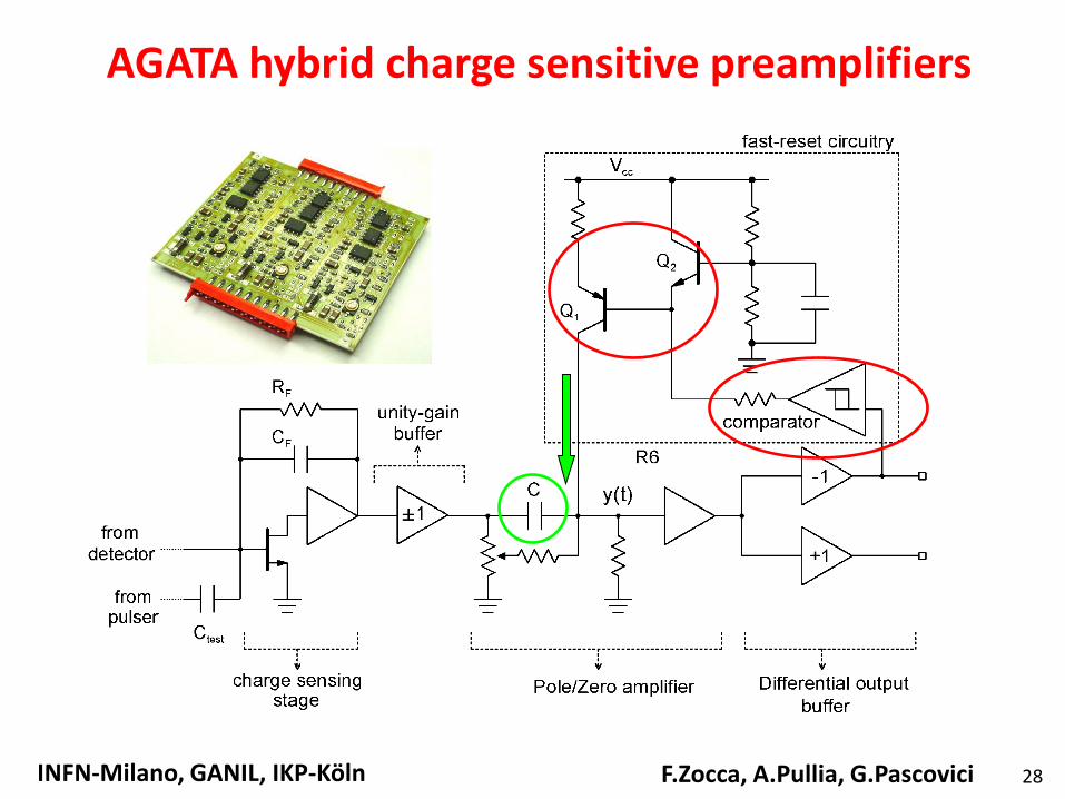
AGATA hybrid charge sensitive preamplifiers
F.Zocca, A.Pullia, G.Pascovici INFN-Milano, GANIL, IKP-Köln 28

O
EVVkTbTbE 211
2
21
E = energy of the large signal
T = reset time
contribution of the tail due to previous events
Time-Over-Threshold (TOT) technique
V1 , V2 = pre-pulse and post-pulse baselines
b1 , b2 , k1 , E0 = fitting parameters
second-order time-energy relation offset term
Within ADC range standard “pulse-height mode” spectroscopy
Beyond ADC range new “reset mode” spectroscopy
F.Zocca, A.Pullia, G.Pascovici 29
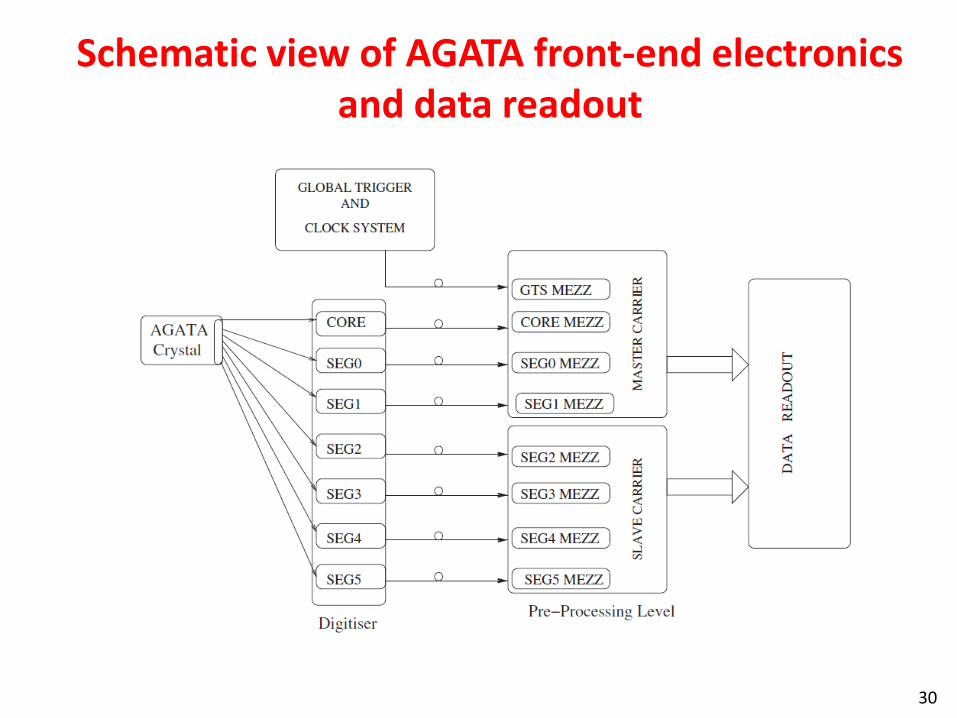
Schematic view of AGATA front-end electronics and data readout
30
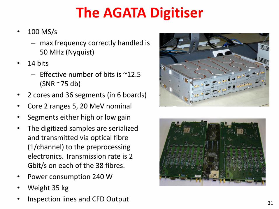
The AGATA Digitiser • 100 MS/s
– max frequency correctly handled is 50 MHz (Nyquist)
• 14 bits
– Effective number of bits is ~12.5 (SNR ~75 db)
• 2 cores and 36 segments (in 6 boards)
• Core 2 ranges 5, 20 MeV nominal
• Segments either high or low gain
• The digitized samples are serialized and transmitted via optical fibre (1/channel) to the preprocessing electronics. Transmission rate is 2 Gbit/s on each of the 38 fibres.
• Power consumption 240 W
• Weight 35 kg
• Inspection lines and CFD Output 31
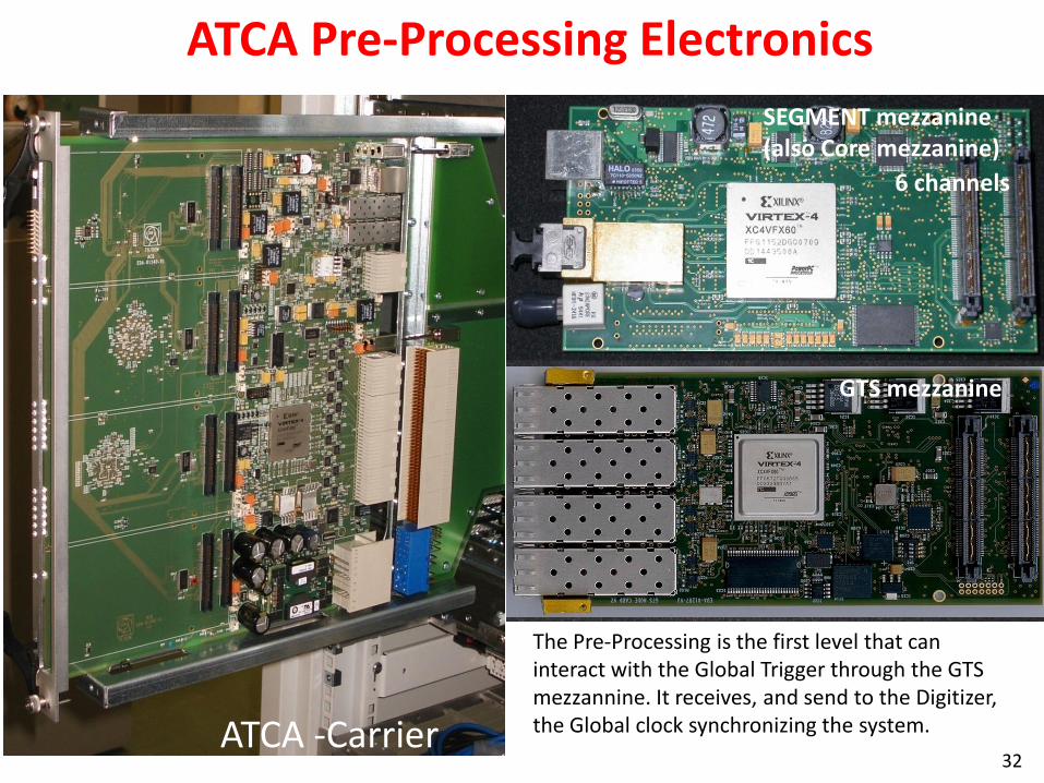
ATCA Pre-Processing Electronics
ATCA -Carrier
SEGMENT mezzanine (also Core mezzanine)
6 channels
GTS mezzanine
The Pre-Processing is the first level that can interact with the Global Trigger through the GTS mezzannine. It receives, and send to the Digitizer, the Global clock synchronizing the system.
32
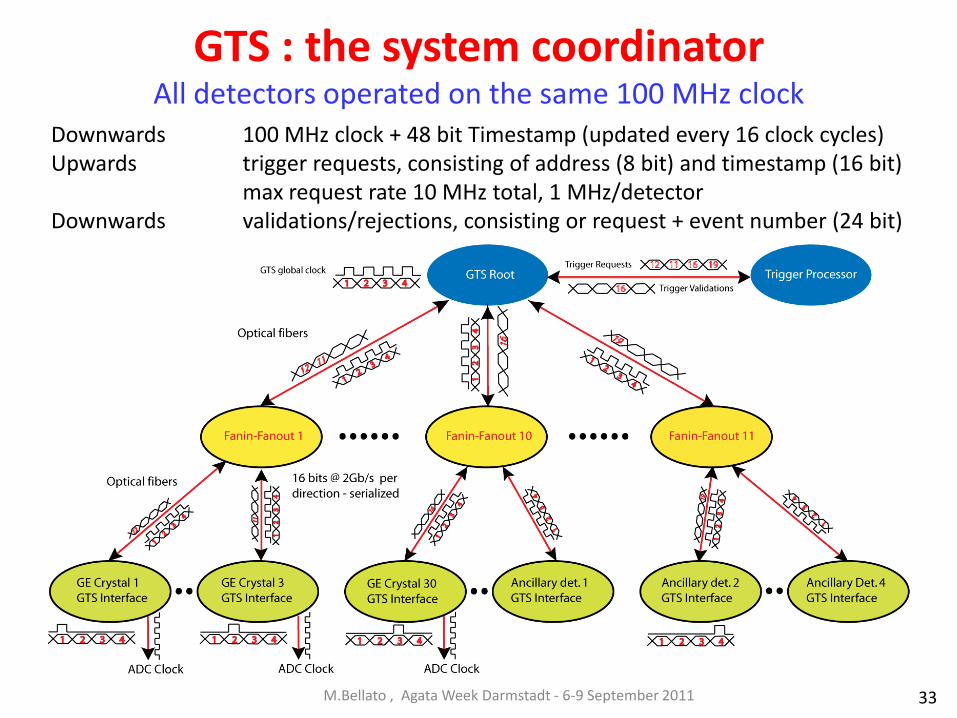
GTS : the system coordinator All detectors operated on the same 100 MHz clock
M.Bellato , Agata Week Darmstadt - 6-9 September 2011
Downwards 100 MHz clock + 48 bit Timestamp (updated every 16 clock cycles) Upwards trigger requests, consisting of address (8 bit) and timestamp (16 bit) max request rate 10 MHz total, 1 MHz/detector Downwards validations/rejections, consisting or request + event number (24 bit)
33
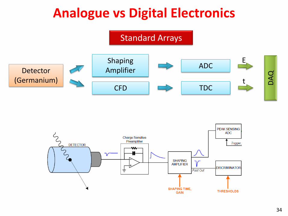
Analogue vs Digital Electronics
Detector (Germanium)
Shaping Amplifier
CFD
DA
Q
E
t
ADC
TDC
Standard Arrays
34

Performance comparable to best analog electronics. Higher count rate capabilities
FADC
MWD
DCFD
Filters
DA
Q
E
t PSA
Trac
kin
g
E
t
x,y,z
E
t
AGATA
Segment Detector Array
Detector (Germanium)
Analogue vs Digital Electronics
35
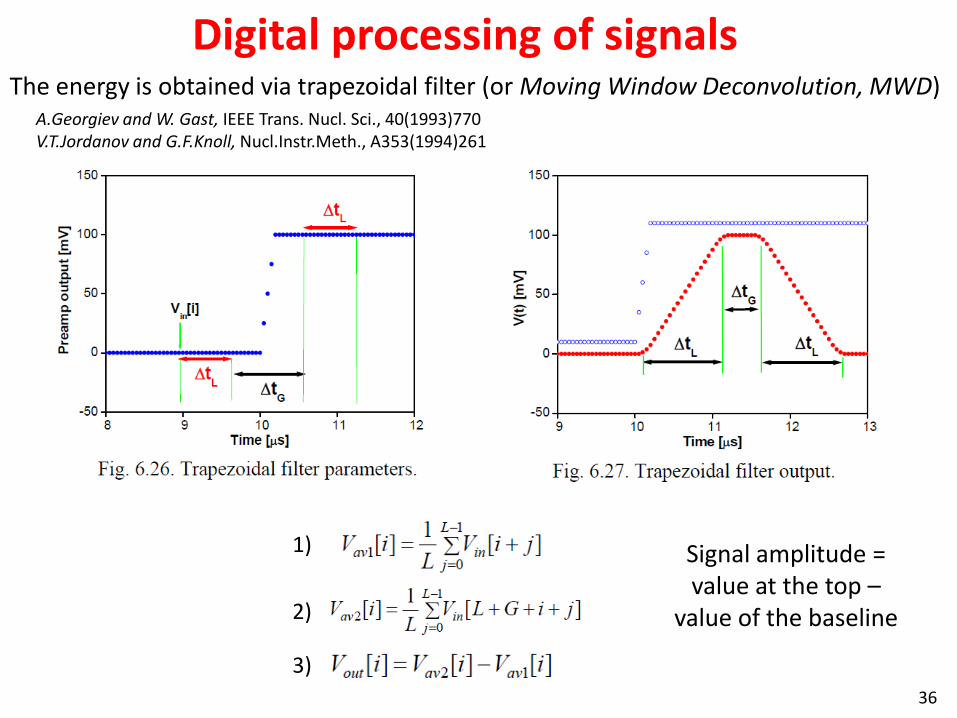
1)
2)
3)
Digital processing of signals The energy is obtained via trapezoidal filter (or Moving Window Deconvolution, MWD)
A.Georgiev and W. Gast, IEEE Trans. Nucl. Sci., 40(1993)770 V.T.Jordanov and G.F.Knoll, Nucl.Instr.Meth., A353(1994)261
Signal amplitude = value at the top –
value of the baseline
36
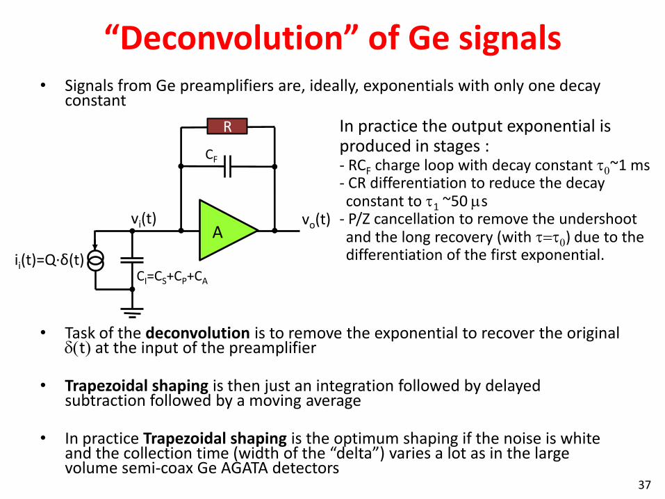
• Signals from Ge preamplifiers are, ideally, exponentials with only one decay constant
• Task of the deconvolution is to remove the exponential to recover the original
dt at the input of the preamplifier
• Trapezoidal shaping is then just an integration followed by delayed subtraction followed by a moving average
• In practice Trapezoidal shaping is the optimum shaping if the noise is white and the collection time (width of the “delta”) varies a lot as in the large volume semi-coax Ge AGATA detectors
“Deconvolution” of Ge signals
CF
ii(t)=Q·δ(t) CI=CS+CP+CA
A
R
vi(t) vo(t)
In practice the output exponential is produced in stages : - RCF charge loop with decay constant t0~1 ms - CR differentiation to reduce the decay constant to t1 ~50 ms
- P/Z cancellation to remove the undershoot and the long recovery (with tt0) due to the differentiation of the first exponential.
37

time [10ns]
30 kHz "nominal"
(front) segment
core
Signal processing at high counting rates
38

time [10ns]
30 kHz "nominal"
Signal processing at high counting rates
core
MWD amplitude: risetime 5us risetime 2.5us
38
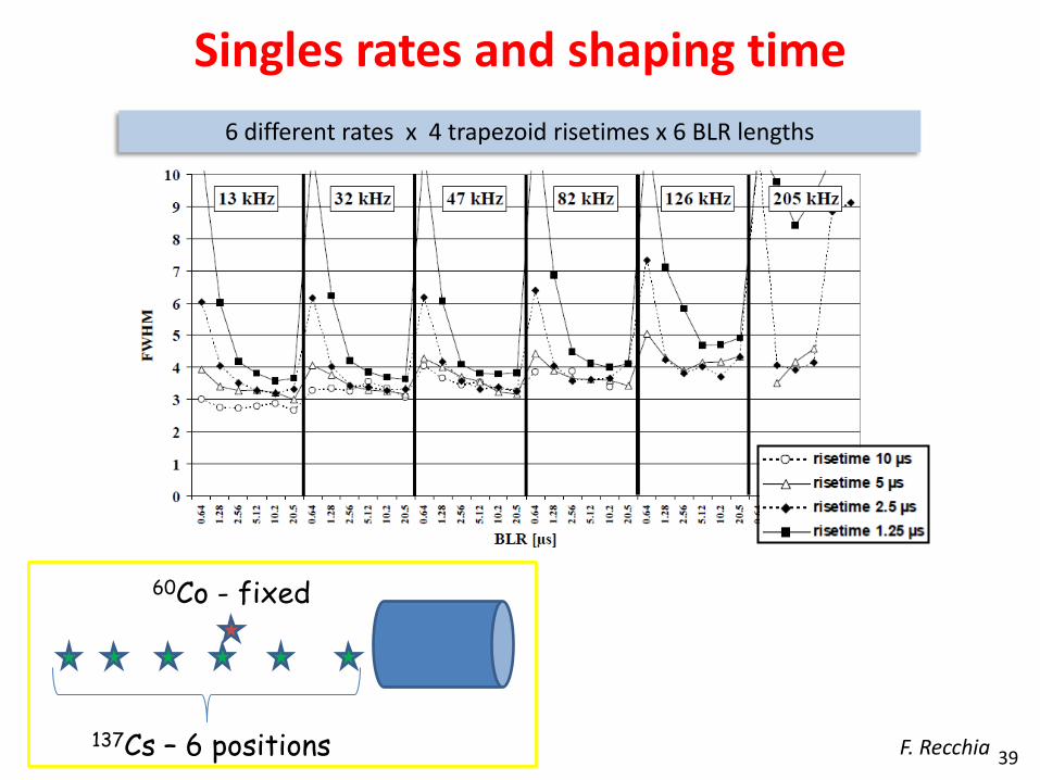
Singles rates and shaping time
60Co - fixed
137Cs – 6 positions
6 different rates x 4 trapezoid risetimes x 6 BLR lengths
F. Recchia 39
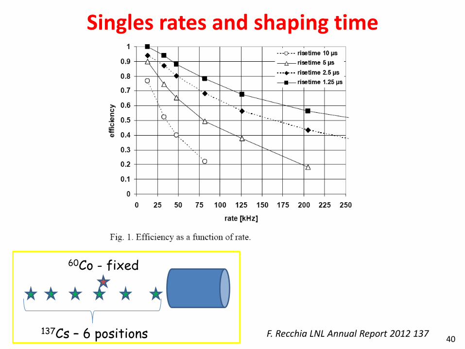
Singles rates and shaping time
60Co - fixed
137Cs – 6 positions F. Recchia LNL Annual Report 2012 137 40
AGATA Data Processing
(from raw data to reconstructed "good" gamma rays)
Offline data processing = Online data processing
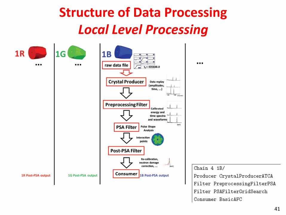
Structure of Data Processing Local Level Processing
41
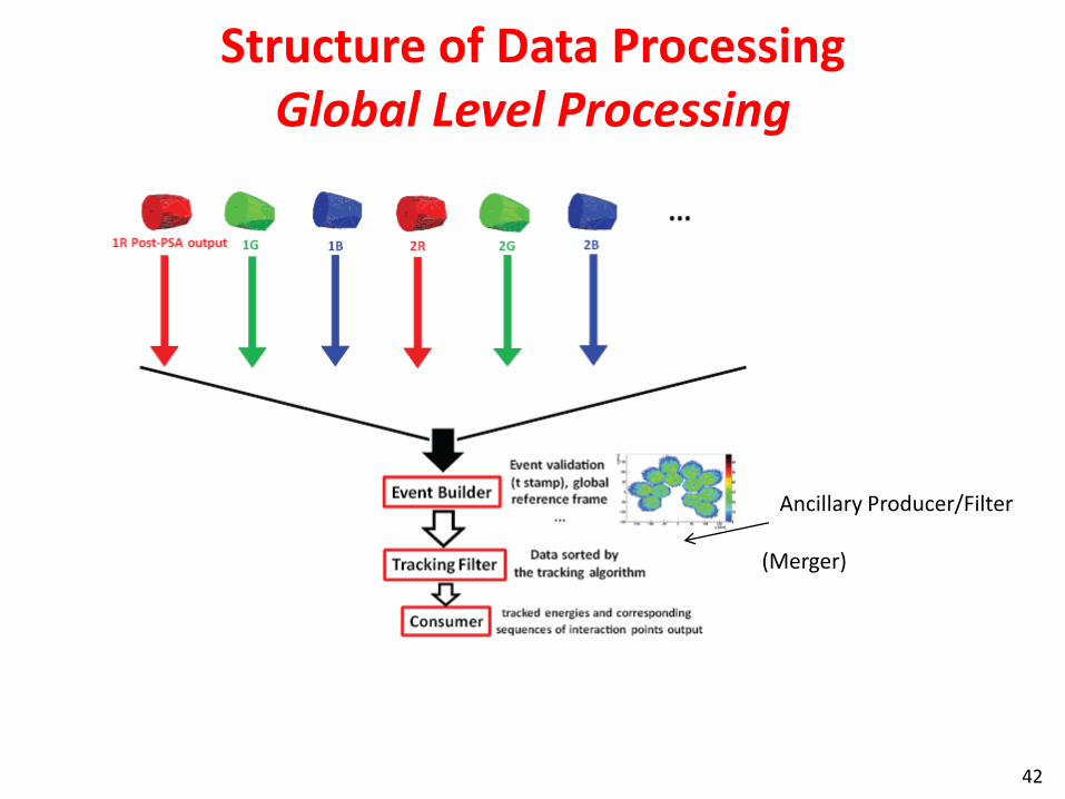
Structure of Data Processing Global Level Processing
Ancillary Producer/Filter
(Merger)
42
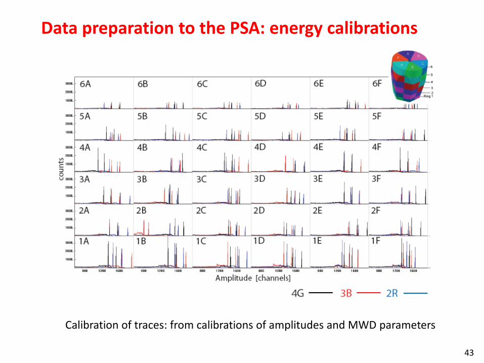
Data preparation to the PSA: energy calibrations
Calibration of traces: from calibrations of amplitudes and MWD parameters
43
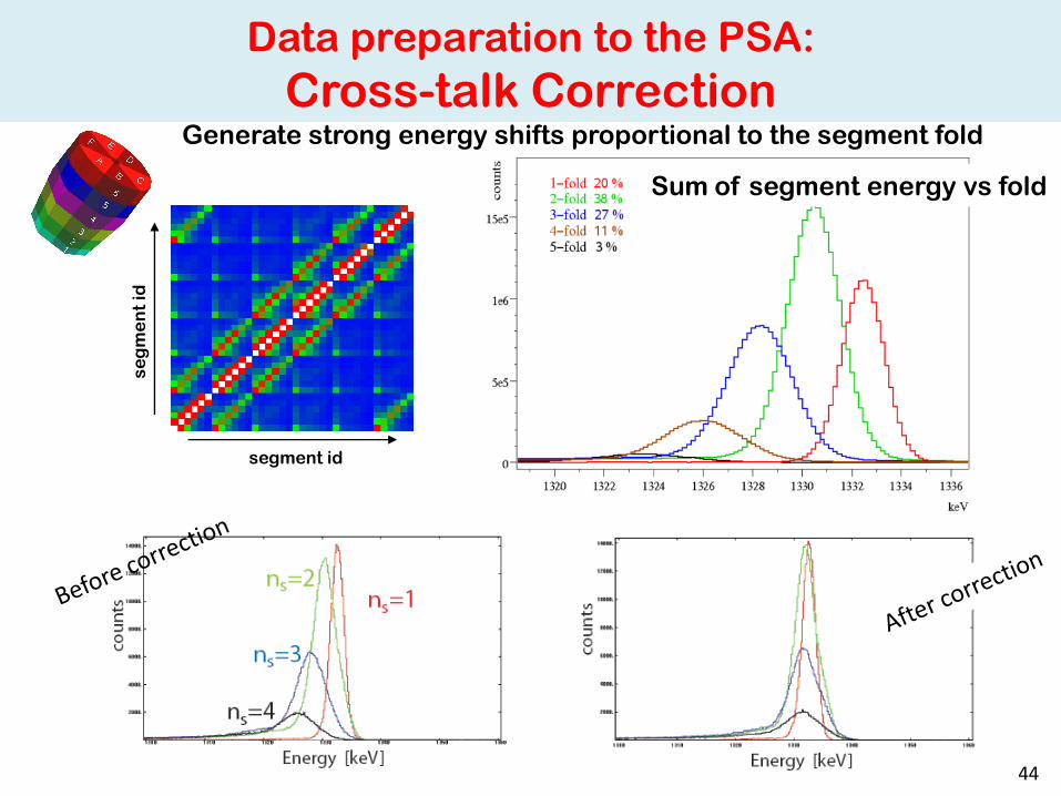
Data preparation to the PSA:
Cross-talk Correction
Sum of segment energy vs fold
segment id
se
gm
en
t id
Generate strong energy shifts proportional to the segment fold
44
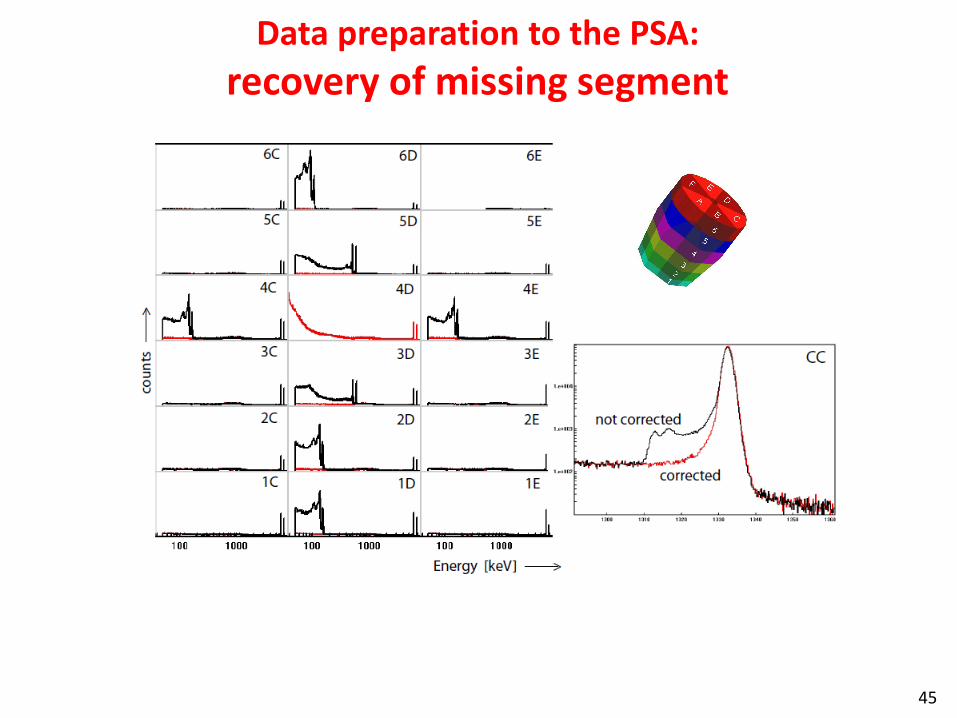
Data preparation to the PSA:
recovery of missing segment
45

Some results from the commissioning runs in GANIL
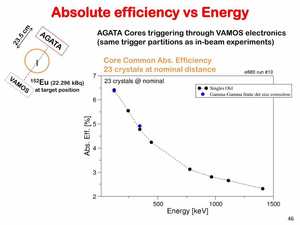
Absolute efficiency vs Energy
AGATA Cores triggering through VAMOS electronics
(same trigger partitions as in-beam experiments)
152Eu (22.296 kBq)
at target position
Core Common Abs. Efficiency
23 crystals at nominal distance
46
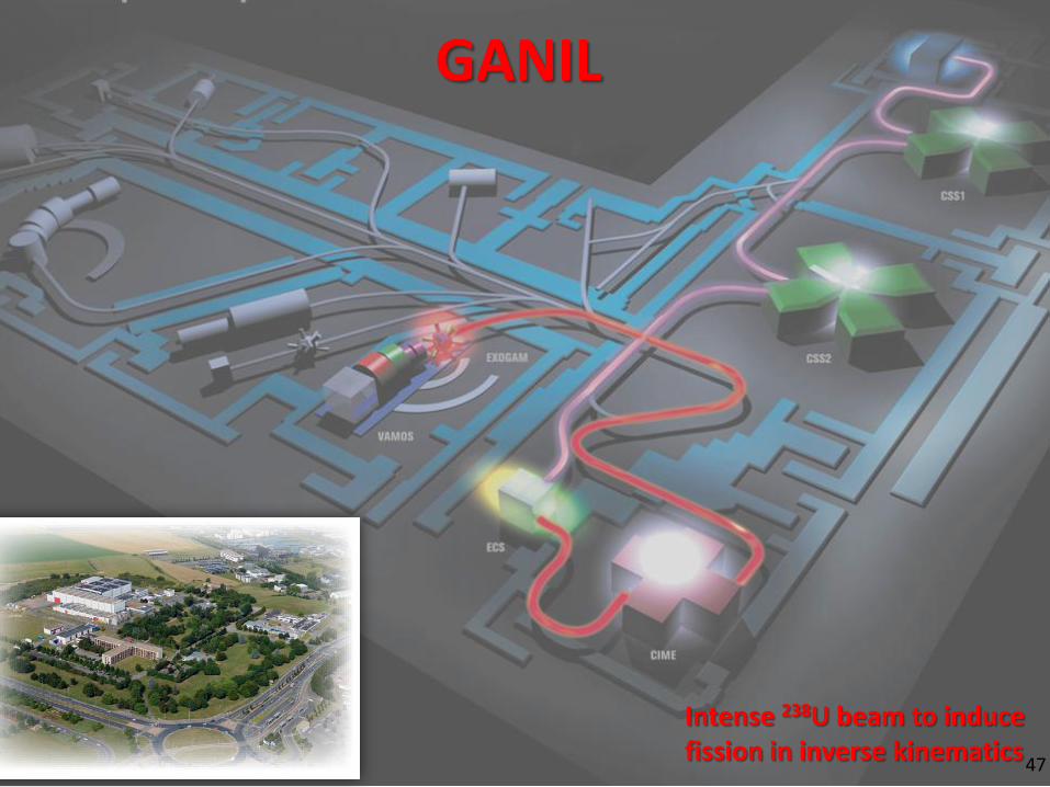
GANIL
Intense 238U beam to induce fission in inverse kinematics
47
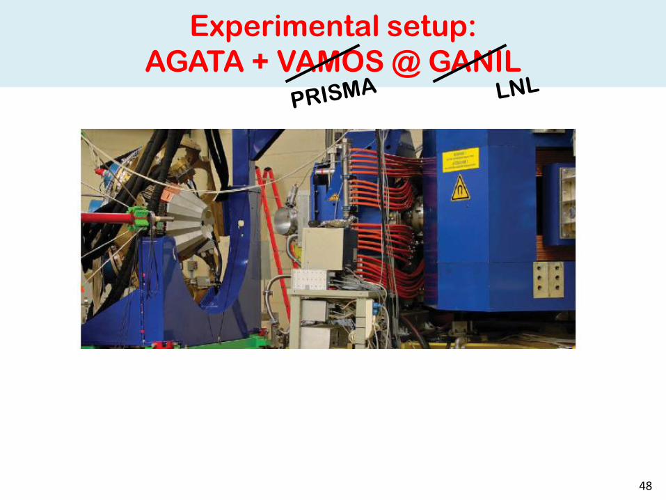
Experimental setup:
AGATA + VAMOS @ GANIL
48
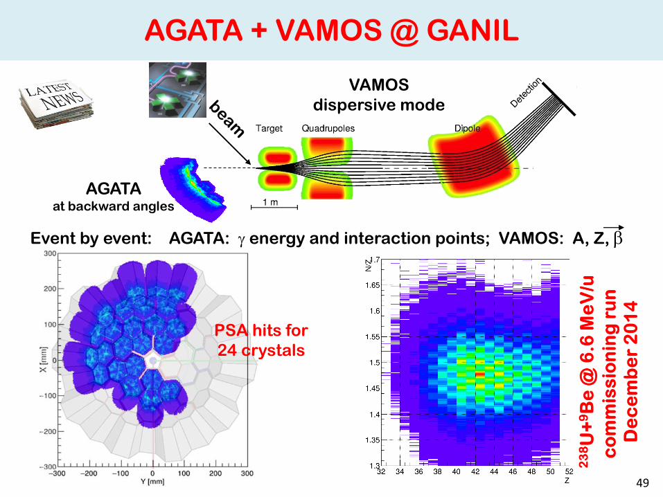
VAMOS
dispersive mode
AGATA at backward angles
AGATA + VAMOS @ GANIL
Event by event: AGATA: g energy and interaction points; VAMOS: A, Z, b
PSA hits for
24 crystals
49
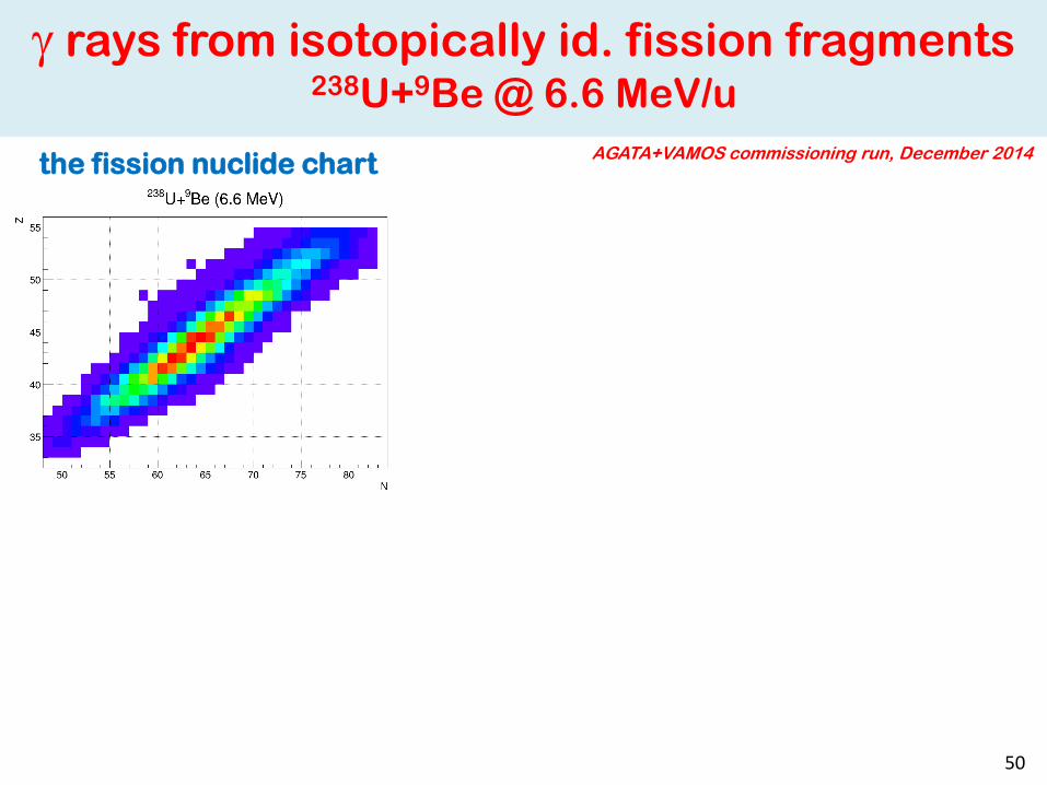
g rays from isotopically id. fission fragments 238U+9Be @ 6.6 MeV/u
the fission nuclide chart AGATA+VAMOS commissioning run, December 2014
50
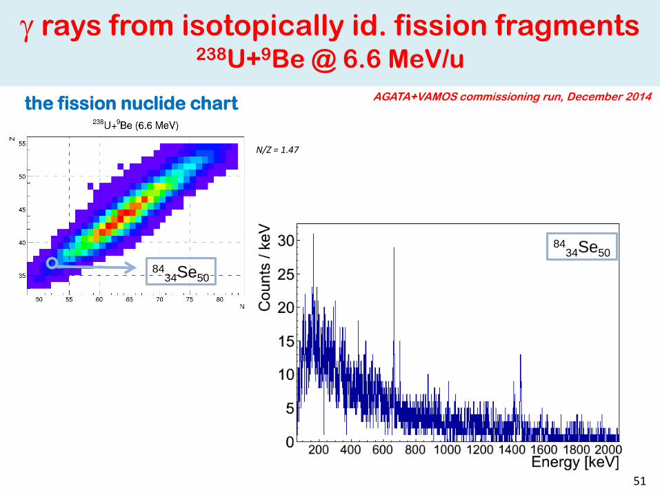
8434Se50
8434Se50
N/Z = 1.47
g rays from isotopically id. fission fragments 238U+9Be @ 6.6 MeV/u
AGATA+VAMOS commissioning run, December 2014 the fission nuclide chart
51

9036Kr54
9036Kr54
N/Z = 1.50
g rays from isotopically id. fission fragments 238U+9Be @ 6.6 MeV/u
AGATA+VAMOS commissioning run, December 2014 the fission nuclide chart
51
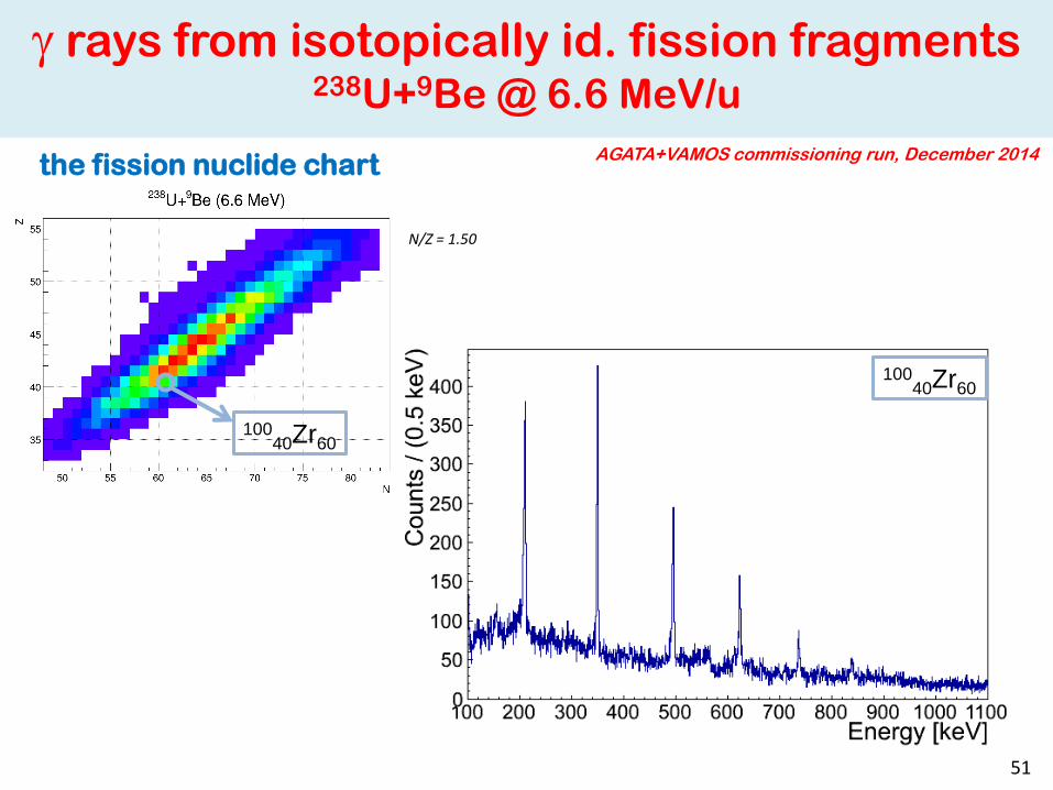
10040Zr60
10040Zr60
N/Z = 1.50
g rays from isotopically id. fission fragments 238U+9Be @ 6.6 MeV/u
AGATA+VAMOS commissioning run, December 2014 the fission nuclide chart
51
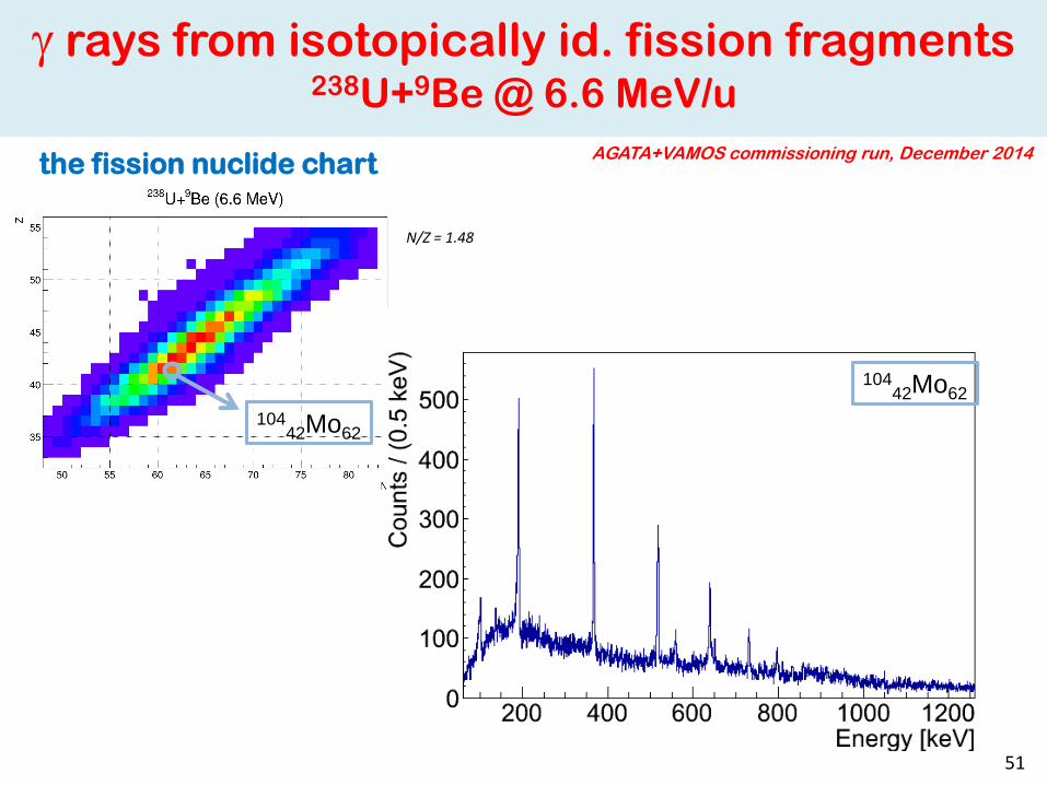
10442Mo62
10442Mo62
N/Z = 1.48
g rays from isotopically id. fission fragments 238U+9Be @ 6.6 MeV/u
AGATA+VAMOS commissioning run, December 2014 the fission nuclide chart
51

10442Mo62
10442Mo62
N/Z = 1.48
g rays from isotopically id. fission fragments 238U+9Be @ 6.6 MeV/u
AGATA+VAMOS commissioning run, December 2014 the fission nuclide chart
g-g matrix
gate on 2+ 0+
52
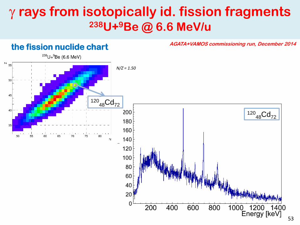
12048Cd72
12048Cd72
N/Z = 1.50
g rays from isotopically id. fission fragments 238U+9Be @ 6.6 MeV/u
AGATA+VAMOS commissioning run, December 2014 the fission nuclide chart
53
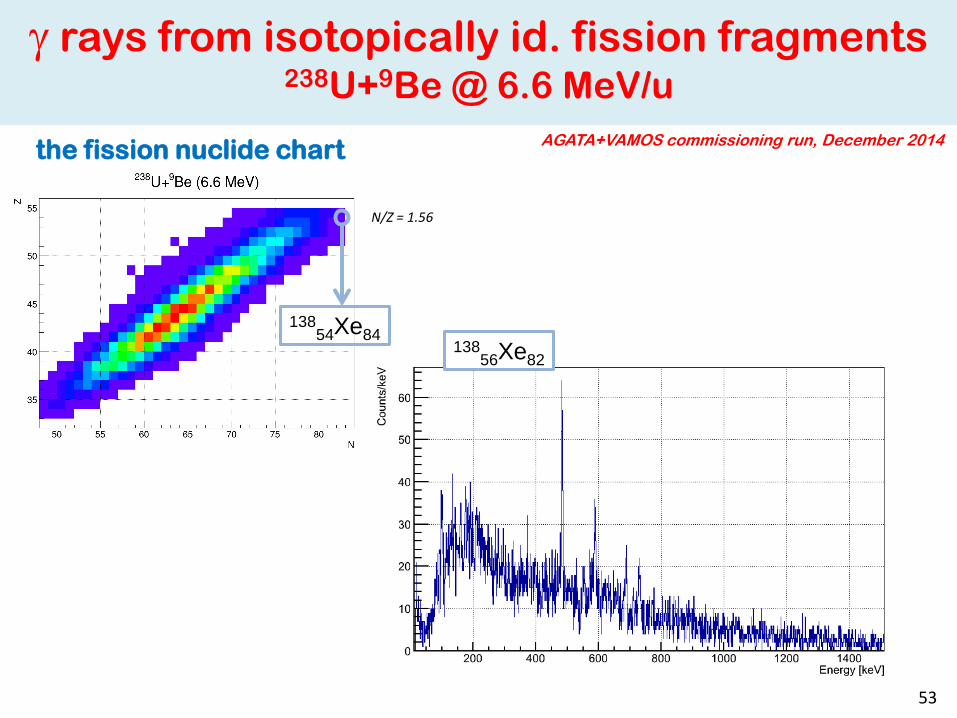
13854Xe84
13856Xe82
N/Z = 1.56
g rays from isotopically id. fission fragments 238U+9Be @ 6.6 MeV/u
AGATA+VAMOS commissioning run, December 2014 the fission nuclide chart
53
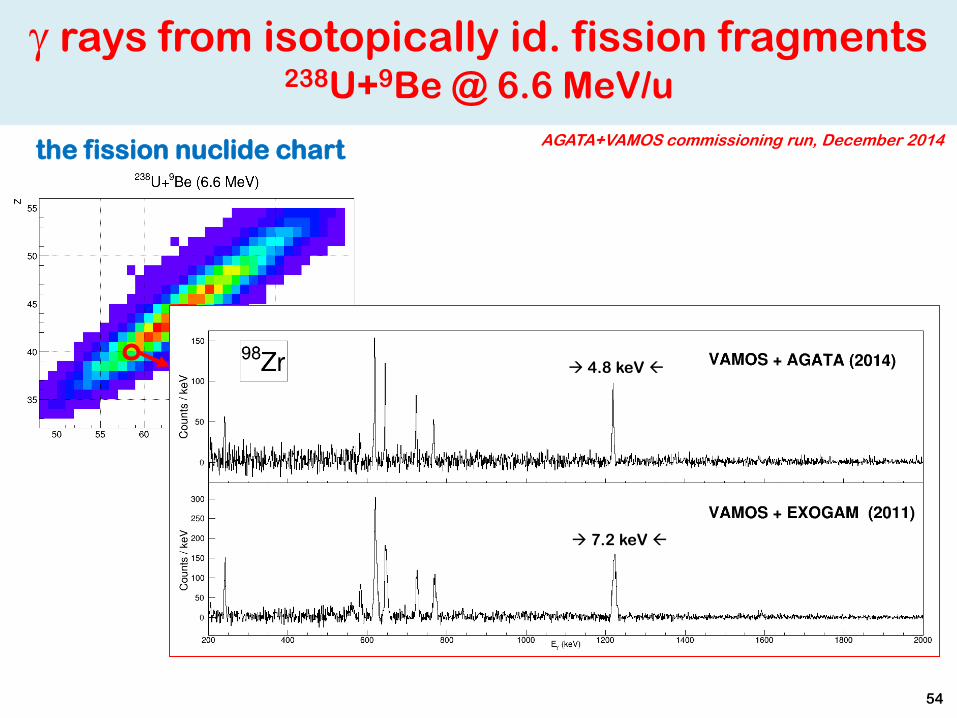
g rays from isotopically id. fission fragments 238U+9Be @ 6.6 MeV/u
AGATA+VAMOS commissioning run, December 2014 the fission nuclide chart
54
4.8 keV
7.2 keV
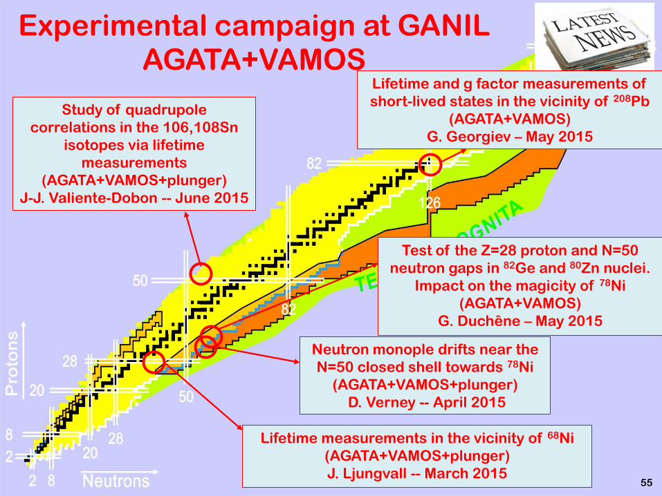
Experimental campaign at GANIL AGATA+VAMOS
Lifetime measurements in the vicinity of 68Ni
(AGATA+VAMOS+plunger)
J. Ljungvall -- March 2015
Neutron monople drifts near the
N=50 closed shell towards 78Ni
(AGATA+VAMOS+plunger)
D. Verney -- April 2015
Test of the Z=28 proton and N=50
neutron gaps in 82Ge and 80Zn nuclei.
Impact on the magicity of 78Ni
(AGATA+VAMOS)
G. Duchêne – May 2015
Study of quadrupole
correlations in the 106,108Sn
isotopes via lifetime
measurements
(AGATA+VAMOS+plunger)
J-J. Valiente-Dobon -- June 2015
55
Lifetime and g factor measurements of
short-lived states in the vicinity of 208Pb
(AGATA+VAMOS)
G. Georgiev – May 2015