Number Theory

And Related Topics

NUMBER THEORY

AND RELATED TOPICS

Papers presented at the Ramanujan Colloquium, Bombay 1988, by

ASKEY BALASUBRAMANIAN BERNDT

BRESSOUD HEATH-BROWN IWANIEC

KUZNETSOV RAGHAVAN RAMACHANDRA

RAMANATHAN RANGACHARI RANKIN SATAKE

SCHMIDT SELBERG SHOREY ZAGIER

Published for the

TATA INSTITUTE OF FUNDAMENTAL RESEARCH,

BOMBAY

OXFORD UNIVERSITY PRESS

1989

Oxford University Press, Walton Street, Oxford OXZ 6DP

NEW YORK TORONTO

DELHI BOMBAY CALCUTTA MADRAS KARACHI

PETALING JAYA SINGAPORE HONGKONG TOKYO

NAIROBI DAR ES SALAAM

MELBOURNE AUCKLAND

and associates in

BERLIN IBADAN

c© Tata Institute of Fundamental Research, 1989

ISBN 0 19 562367 3

Typeset and Printed in India by B. A. Gala,

Anamika Trading Co., Dadar, Bombay 400 028

and published by S. K. Mookerjee, Oxford University Press,

Oxford House, Apollo Bunder, Bombay 400 039.

Ramanujan Birth Centenary International

Colloquium on Number Theory and Related

Topics

Bombay, 4-11 January 1988

REPORT

An International Colloquium on Number Theory and related topics 1

was held at the Tata Institute of Fundamental Research, Bombay during

4-11 January, 1988, to mark the birth centenary of Srinivasa Ramanujan.

The purpose of the Colloquium was to highlight recent developments in

Number Theory and related topics, especially those related to the work

of Ramanujan “such as the Circle method, Sieve methods and Combi-

natorial techniques in Number theory, Partition congruences, Rogers -

Ramanujan identities, Lacunarity of power series, Hypergeometric se-

ries and Special functions, Complex multiplication, Hecke theory etc.”

The Colloquium was organized by the Tata Institute of Fundamen-

tal Research with co-sponsorship from the International Mathematical

Union. Financial support was received from the International Mathe-

matical Union and the Sir Dorabji Tata Trust, as in former years. The

organizing committee of the Colloquium consisted of Professors M.S.

Narasimhan, S. Raghavan, M.S. Raghunathan, K. Ramachandra and

C.S. Seshadri and Dr. S.S. Rangachari. The International Mathematical

Union was represented on the committee by Professors M.S. Narasimhan

and C.S. Seshadri.

The following mathematicians delivered one-hour addresses at the

Colloquium:

REPORT

G.E. Andrews, R. Askey, B. C. Berndt, D. M. Bressoud, D. R.

Heath-Brown, N. V. Kuznetsov, K. Ramachandra, K. G. Ramanathan,

S. S. Rangachari, R. A. Rankin, I. Satake, W. M. Schmidt, A. Selberg,

J. P. Serre, T. N. Shorey and D. Zagier.

Professor H. Iwaniec could not attend the Colloquim but sent a paper

for inclusion in the Proceedings.

Besides members of the School of Mathematics of the Tata Institute

of Fundamental Research, mathematicians from universities and educa-

tional institutions in India, France, Canada, Japan and the United States

of America were also invited to attend the Colloquium.

The social programme for the Colloquium included a tea-party on

4 January, a classical Indian dance performance (Bharatanatyam) on 6

January, a film show and a dinner-party at the Institute on 7 January,

a violin recital (Hindustani music) on 8 January, an excursion to the

Elephanta Caves on 9 January and a farewell dinner-party on 10 January

1988.

Contents

1. R. Askey : Variants of Clausen’s formula for the

square of a special 2F1

1–14

2. R. Balasubramanian : and K. Ramachandra :

Titchmarsh’s phenomenon for ζ(s)

15–26

3. B. C. Berndt : Ramanujan’s formulas for

Eisenstein series

27–34

4. D. M. Bressoud : On the proof of Andrews’

q-Dyson conjecture

35–44

5. D. R. Heath-Brown : Weyl’s inequality, Waring’s

problem and Diophantine approximation

45–51

6. H. Iwaniec : The circle method and the Fourier

coefficients of modular forms

52–62

7. N. V. Kuznetsov : Sums of Kloosterman sums and

the eighth power moment of the Riemann zeta

function

63–137

8. S. Raghavan : and S. S. Rangachari : On

Ramanujan’s elliptic integrals and modular

identities

138-175

9. K. G. Ramanathan : On some theorems stated by

Ramanujan

176–188

10. R. A. Rankin : The adjoint Hecke operator II 189–210

11. I. Satake : On zeta functions associated with

self-dual homogeneous cones

211-231

12. W. M. Schmidt : The number of rational

approximations to algebraic numbers and the

number of solutions of norm form equations

232–240

13. A. Selberg : Linear operators and automorphic

forms

241–257

14 T. N. Shorey : Some exponential Diophantine

equations II

258–273

15. D. Zagier : The dilogarithm function in geometry

and number theory

274–295

VARIANTS OF CLAUSEN’S FORMULA

FOR THE SQUARE OF A SPECIAL2F1

By RICHARD ASKEY*

1 Introduction

One of the most striking series Ramanujan [10] found is 1

9801

2π√

2=

∞∑

n=0

[1103 + 26390n](4n)!

[n!]4(4.99)4n. (1.1)

The first proofs of 1.1 have been given recently by Jonathan and Peter

Borwein [3] and by David and Gregory Chudnovsky [5]. They have

also found other identities of a similar nature, [4], [5]. As they remark,

Clausen’s identity [6]

2F1

a, b

a + b +1

2

; x

2

= 3F2

2a, 2b, a + b

a + b +1

2, 2a + 2b

; x

(1.2)

plays a central role in the derivation of (1.1). Here

pFp

a1, . . . , ap

b1, . . . , bq

; x

=

∞∑

n=0

(a1)n . . . (ap)nxn

(b1)n . . . (bq)nn!(1.3)

with

(a)n = Γ(n + a)/Γ(a). (1.4)

*Supported in part by an NSF grant, in part by a sabbatical leave from the University

of Wisconsin, and in part by funds the Graduate School of the University of Wisconsin.

1

2 1 INTRODUCTION

Ramanujan [11] stated an extension of Clausen’s formula

2F1

a, b

c;

1 −√

1 − x

2

2F1

a, b

d;

1 −√

1 − x

2

(1.5)

= 4F3

a, b, (a + b)/2, (c + d)/2

c, d, a + b; x

when c + d = a + b + 1. When c = d and the quadratic transformation

2F1

a, b

(a + b + 1)/2;

1 −√

1 − x

2

= 2F1

a/2, b/2

(a + b + 1)/2; x

is used, the result is (1.2). The first published proof of (1.5) is due to

Bailey [1].

David and Gregory Chudnovsky have been asking me if there are2

other results like Clausen’s formula, where the square of a 2F1 is repre-

sented as a generalized hypergeometric series. There are other instances,

ans one will be given explicitly. The method of deriving it is probably

similar to Ramanujan’s method of deriving Clausen’s formula. As a

warm up, here is how I think Ramanujan derived (1.2).

There are two chapters in Ramanujan’s Second Notebook devoted

to hypergeometric series. The first formula in this first of these two

chapters is the sum of the 2-balanced very well posited 7F6. This is a

fundamental formula, as Ramanujan knew, since he started with it. This

sum is

7F6

a, 1 + (a/2), b, c, d, e,−n

a/2, a + 1 − b, a + 1 − c, a + 1 − d, a + 1 − e, a + 1 − n; 1

(1.6)

=(a + 1)n(a + 1 − b − c)n(a + 1 − b − d)n(a + 1 − c − d)n

(a + 1 − b)n(a + 1 − c)n(a + 1 − d)n(a + 1 − b − c − d)n

and

e = 2a + 1 + n − b − c − d, (1.7)

3

The phrases very well poised and 2-balanced are defined as follows.

A series

p+1Fp

a0, a1, . . . , ap

b1, . . . , bp

; x

(1.8)

is said to be k-balanced if x = 1, if one of the numerator parameters is a

negative integer, and if

k +

p∑

j=0

a j =

p∑

j=1

b j.

The series 1.8 is said to be well poised if a0+1 = a1+b1 = . . . = ap+bp.

It is very well poised if it is well poised and if a1 = b1 + 1. Observe that

the condition (1.7) comes from the series being 2-balanced.

Dougall [7] published the first derivation of (1.6). Ramanujan’s dis-

covery was probably later, but not much later.

To derive Clausen’s formula, first consider

2F1

a, b

c; x

2

=

∞∑

n=0

xnn

∑

k=0

(a)k(b)k(a)n−k(b)n−k

(c)kk!(c)n−k(n − k)!(1.9)

=

∞∑

n−0

(a)n(b)n

(c)nn!4F3

− n, a, b, 1 − n − c

1 − n − a 1 − n − b, c; 1

xn.

The 4F3 series that multiplies xn in the expression in (1.9) is well 3

poised. While a well poised 3F2 at x = 1 can be summed, and a very

well poised 5F4 can be summed when x = 1, a general well poised 4F3

at x = 1 cannot be summed. However when the series is 2-balanced it

can be summed. To see this, first reduce the very well poised 7F6 to a

well poised 4F3. This is done by setting d = a/2, c = (a + 1)/2. Then

(1.6) becomes

4F3

a, b, e,−n

a + 1 − b, a + 1 − e, a + 1 + n; 1

(1.10)

=(a + 1)n((a + 1 − 2b)/2)n((a + 2 − 2b)/2)n(1/2)n

(a + 1 − b)n((a + 1)/2)n((a + 2)/2)n((1 − 2b)/2)n

4 2 THE FOUR BALANCED VERY WELL POISED 7F6

=(a + 1)n(a + 1 − 2b)2n(1/2)n

(a + 1 − b)n(a + 1)2n((1 − 2b)/2)n

=(a + 1 − 2b)2n(1/2)n

(a + 1 − b)n(a + n + 1)n((1 − 2b)/2)n

=Γ(a + 1 − 2b + 2n)Γ(n + 1/2)Γ(a + 1 − b)Γ(a + n + 1)Γ(1/2 − b)

Γ(a + 1 − 2b)Γ(1/2)Γ(a + 1 − b + n)Γ(a + 2n + 1)Γ((1/2) − b + n)

This last expression can be used when a = −k. Then

4F3

− k, b, e,−n

1 − b − k, 1 − e − k, 1 + n − k; 1

=Γ(1 − k − 2b + 2n)Γ(1/2 + n)Γ((1/2) − b)Γ(1 − b − k)Γ(1 + n − k)

Γ(1 − k − 2b)Γ(1 − k + 2n)Γ(1/2)Γ(1 − k − b + n)Γ((1/2) − b + n).

holds for n = k, k + 1, . . ., and is a rational function of n, so it holds

when n is replaced by continuous parameter −a. The result is

4F3

− k, a, b, e

1 − a − k, 1 − b − k, 1 − e − k; 1

=(2a)k(2b)k(a + b)k

(a)k(b)k(2a + 2b)k

(1.11)

after simplification. Recall that this series is 2-balanced, so e = −a−b−k + (1/2).

One can take a = −k in (1.6) and then remove the restriction that

one of the other parameters is a negative integer. However setting c =

(1 − k)/2, d = −k/2 to obtain the 4F3 leads to an indeterminate form, so

it is better to reduce to a 4F3 initially before letting a→ −k.4

Both (1.10) and (1.11) are 2-balanced well poised series, but they

are different in that different parameters are used to terminate the series.

When (1.11) is used in (1.9), he result is Clausen’s formula (1.2).

2 The four balanced very well poised 7F6

To find another formula like Clausen’s identity, we can look for another

well poised series that can be summed. The obvious candidate is the

4-balanced very well poised 7F6. There are two natural ways to sum

5

this series. One is an easy consequence of (1.6), so it is a derivation

Ramanujan could have easily given. We start with it. Set

fk(b) =(b)k(e)k

(a + 1 − b)k(a + 1 − e)k

(2.1)

and use the 2-balanced condition

e = 2a + 1 + n − b − c − d. (2.2)

A routine calculation gives

b(a − b) fk(b + 1) − (e − 1)(a + 1 − e) fk(b)

=(b)k(e − 1)k

(a + 1 − b)k(a + 2 − e)k

[b(a − b) − (e − 1)(a + 1 − e)].

Observe that the last factor is

b(a − b) − (2a + n − b − c − d)(b + c + d − n − a)

= (n +3a

2− b − c − d +

a

2)(n +

3a

2− b − c − d −

a

2) − (b −

a

2−

a

2)(b −

a

2+

a

2)

= (n +3a

2− b − c − d)2 − (b −

a

2)2= (n + 2a − 2b − c − d)(n + a − c − d);

so

(n + 2a − 2b − c − d)(n + a − c − d)×

× 7F6

a,a

2+ 1, b, c, d, e − 1,−n

a

2, a + 1 − b, a + 1 − c, a + 1 − d, a + 2 − e, a + 1 + n

; 1

= b(a − b)7F6

a,a

2+ 1, b + 1, c, d, e − 1,−n

a

2, a − b, a + 1 − c, a + 1 − d, a + 2 − e, a + 1 + n

; 1

− (e − 1)(a + 1 − e)×

× 7F6

a,a

2+ 1, b, c, d, e,−n

a

2, a + 1 − b, a + 1 − c, a + 1 − d, a + 1 − e, a + 1 + n

; 1

6 2 THE FOUR BALANCED VERY WELL POISED 7F6

=b(a − b + n)(a + 1)n(a − b − c)n(a − b − d)n(a + 1 − c − d)n

(a + 1 − b)n(a + 1 − c)n(a + 1 − d)n(a − b − c − d)n

− (2a + n − b − c − d)(b + c + d − a)×

×(a + 1)n(a + 1 − b − c)n(a + 1 − b − d)n(a + 1 − c − d)n

(a + 1 − b)n(a + 1 − c)n(a + 1 − d)n(a − b − c − d)n

or shifting e up by 1 and doing some algebra:5

7F6

a,a

2+ 1, b, c, d, e,−n

a

2, a + 1 − b, a + 1 − c, a + 1 − d, a + 1 − e, a + 1 + n

; 1

(2.3)

=(a + 1)n(a − b − c)n(a − b − d)n(a − c − d)n

(a + 1 − b)n(a + 1 − c)n(a + 1 − d)n(a − b − c − d)n

×

×

[

1 +n(n + 2a − b − c − d)(a − b − c − d)

(a − b − c)(a − b − d)(a − c − d)

]

when the series is 4-balanced, or equivalently when

e = 2a + n − b − c − d. (2.4)

The second natural way to derive (2.3) uses a more complicated

formula than (1.6), but the calculations from the starting formula are

easier, and one can see how to extend the sum to the very well poised

2k-balanced series. The starting formula is Whipple’s transformation

[14] between a very well poised 7F6 and a balanced 4F3:

7F6

a,a

2+ 1, b, c, d, e,−n

a

2, a + 1 − b, a + 1 − c, a + 1 − d, a + 1 − e, a + 1 + n

; 1

(2.5)

=(a + 1)n(a + 1 − b − c)n

(a + 1 − b)n(a + 1 − c)n4F3

− n, a + 1 − d − e, b, c

b + c − n − a, a + 1 − d, a + 1 − e; 1

.

When e = 2a + n − b − c − d, the 4F3 on the right is

4F3

−n, b + c + 1 − n − a, b, c

b + c − n − a, a + 1 − d, b + c + d + 1 − n − a; 1

7

=

n∑

k=0

(−n)k(b)k(c)k

(a + 1 − d)k(b + c + d + 1 − n − a)kk!·

(k + b + c − n − a)

(b + c − n − a)

= 3F2

− n, b, c

a + 1 − d, b + c + d + 1 − n − a; 1

+

+(−n)bc

(a + 1 − d)(b + c − n − a)(b + c + d + 1 − n − a)×

×3F2

1 − n, b + 1, c + 1

a + 2 − d, b + c + d + 2 − n − a

; 1

The second 3F2 is balanced, and so can be summed using the Pfaff- 6

Saalschutz sum

3F2

− n, b, c

d, 1 + b + c − n − d

; 1 =(d − b)n(d − c)n

(d)n(d − b − c)n

. (2.6)

The first 3F2 is two balanced, and so can be written as the sum of 2

terms by use of the transformation formula:

3F2

− n, a, b

c, d; 1

=(c − a)n(c − b)n

(c)n(c − a − b)n

× (2.7)

× 3F2

− n, a, a + b + 1 − n − c − d

a + 1 − n − c, a + 1 − n − d; 1

.

For, when the series on the left of (2.7) is k-balanced, the third numer-

ator parameter in the series on the right is 1 − k; so the series can be

written as the sum of k terms when k = 1, 2, . . .

For those unacquainted with (2.7), an argument giving a q-extension

is in the last section.

These series combine to give another derivation of (2.3) when (2.4)

has been assumed. This method clearly extends to give the sum of the

2k-balanced very well poised 7F6, but the resulting identity is too messy

to be worth stating until it is needed.

8 3 ANOTHER CLAUSEN TYPE IDENTITY.

3 Another Clausen type identity.

To obtain the next Clausen type identity take the 4F3 in (1.9) to be 4-

balanced, or take c = a + b + 3/2. As before, specialize (2.3) by taking

c = a/2, d = (a + 1)/2 and make the series on the left 4-balanced. The

resulting series is

4F3

− n, a, b, e

a + 1 + n, a + 1 − b, a + 1 − e; 1

(3.1)

=(a + 1)n((a − 2b)/2)n((a − 2b − 1)/2)n(− 1

2)n

(a + 1 − b)n((a + 2)/2)n((a + 2)/2)n(− 12− b)n

×

×

1 +n(n + a − b − 1

2)

[(a − 2b)/2][(a − 2b − 1)/2](− 12)

=(a − 2b − 1)2n(− 1

2)n

(a + 1 − b)n(a + n + 1)n(− 12− b)n

1 +4n(n + a − b − 1

2)(2b + 1)

(a + 2b)(a − 2b − 1)

.

The replace a by −k and after the same argument given above, replace7

−n by a. The result is

4F3

− k, a, b, e

1 − a − k, 1 − b − k, 1 − e − k; 1

=(2a)k(2b)k(a + b)k

(a)k(b)k(2a + 2b + 2)k

× A

(3.2)

with A given by

A = 1 +(2 + 4a + 4b + 8ab)k + k2 − k

2(a + b)(2a + 1)(2b + 1)(3.3)

or by

A =k2+ (8ab + 4a + 4b + 1)k + 2(a + b)(2a + 1)(2b + 1)

2(a + b)(2a + 1)(2b + 1)(3.4)

and

e = −k − a − b −1

2. (3.5)

9

Using (3.2) with A given by (3.3) in (1.9), we obtain

2F2

a, b

a + b +3

2

; x

2

= 3F2

2a, 2b, a + b

a + b +3

2, 2a + 2b + 2

; x

(3.6)

+2ab x

(a + b + 1)(a + b + 3/2)3F2

2a + 1, 2b + 1, a + b + 1

a + b +5

2, 2a + 2b + 3

; x

+abx2

2(a + b + 3/2)2(a + b + 5/2)3F2

2a + 2, 2b + 2, a + b + 2

a + b +7

2, 2a + 2b + 4

; x

Using (3.2) with A given by (3.4) gives

2F1

a, b

a + b +3

2

; x

2

= 5F4

2a, 2b, a + b, c + 1, d + 1

a + b +3

2, 2a + 2b + 2, c, d

; x

(3.7)

where c and d are determined by

x2+ (8ab+4a+4b+1)x+2(a+b)(2a+1)(2b+1) = (x+c)(x+d). (3.8)

4 Comments.

After working out the above results, I went to a library to see if they 8

were new. The fact that

2F1

a, b

a + b + n +1

2

; x

2

, n = 0, 1, . . . , (4.1)

is a generalized hypergeomatric series was proved by Goursat [8]. He

also showed that

2F1

a, b

c; x

2

10 4 COMMENTS.

is a generalized hypergeometric series only when c = a + b + n + 12,

n = 0, 1, . . .. His proof that (4.1) is a generalized hypergeometric series

uses Clausen’s formula (1.2), its derivative

2F1

a, b

a + b +1

2

; x

2F1

a + 1, b + 1

a + b +3

2

; x

(4.2)

= 3F2

2a + 1, 2b + 1, a + b + 1

a + b +3

2, 2a + 2b + 1

; x

and the transformation

2F1

a, b

a + b +1

2

; x

= (1 − x)1/22F1

a +1

2, b +

1

2

a + b +1

2

; x

.

Of course Ramanujan knew all of those facts. Goursat also used some

recurrence relations. Ramanujan knew about some of the recurrence re-

lations hypergeometric series satisfy, and almost surely derived some of

his continued fractions from these recurrence relations. However Ra-

manujan did not use recurrence relations as much as he could have, or

as often as he used other properties of hypergeometric series. While

Ramanujan almost surely could have rediscovered Goursat’s result if he

had needed it, it is more likely he would have used an argument like the

one given above. Ramanujan does not seem to have found Whipple’s

transformation formula (2.5). He did find a limiting case with one pa-

rameter missing, but we have not found (2.5) in any of the sheets of his.

If there is another treasure like the sheets in Trinity College, I would not

be surprised in (2.5) is there.

Actually, I would be surprised if Ramanujan was very interested in

Goursat’s result. What he really loved was not general results that could

not be made very explicit, but beautiful formulas. I could imagine Ra-

manujan working out the details in section 3, but the resulting formulas9

are already starting to be messier than those he loved.

11

I sent an outline of the results in sections 2 and 3 to a couple of

people, and George Andrews wrote back that the 4-balanced very well

poised 7F6 sum was found by Lakin [9]. The two proofs given in section

2 are easier than the two Lakin gave, so it is worth including them above.

Lakin also found a basic hypergeometric extension of this sum. The

derivation of his result from the q-extension of Whipple’s formula is the

most natural one, so it will be given in the next section.

5 The 3-balanced very well poised 8ϕ7.

The analogue of Whipple’s transformation formula (2.5) was found by

Watson [13]. It is

8ϕ7

a, q√

a,−q√

a, b, c, d, e, q−n

√a,−√

a,aq

b,

aq

c,

aq

d,

aq

e, aqn+1

; q,a2qn+1

bcde

(5.1)

=(aq; q)n(

aq

bc; q)n

(aq

b; q)n(

aq

c; q)n

4ϕ3

q−n,aq

de, b, c,

aq

d,

aq

e,

bcq−n

a

; q, q

where

(a; q)n = (1 − a)(1 − aq) . . . (1 − aqn−1) (5.2)

and

p+1ϕp

a0, . . . , ap

b1, . . . , bp

; q, x

=

∞∑

k=0

(a0; q)k . . . (ap; q)k xk

(b1; q)k . . . (bp; q)k(q; q)k

. (5.3)

The series (5.3) is called k-balanced at q j if x = q j, one of the

numerator parameters is q−n and a0a1 . . . apqk= b1 . . . bp. It is called

balanced if k = 1 and j = 1. The series (5.3) is well poised if a0q =

a1b1 = . . . = apbp, and very well poised if it is well poised and if

a1 = qb1, a2 = −a1.

12 5 THE 3-BALANCED VERY WELL POISED 8ϕ7.

The sum that corresponds to (1.6) occurs when the 4ϕ3 in (5.1) be-

comes a 3ϕ2 bey setting a2qn+1= bcde, and using

3ϕ2

qn, a, b

c, q1−nabc−1; q, q

=(c/a; q)n(c/b; q)n

(c; q)n(c/ab; q)n

(5.4)

to sum the resulting balanced 3ϕ2. Observe that the balancing condi-

tion is now 1-balanced in the q-case as opposed to 2-balanced in the

hypergeometric case.

The analogue of (2.3) requires a 3-balanced very well poised 8ϕ7 at

q2. To obtain this sum, use (5.1) with

aq

de=

bcq1−n

a(5.5)

The 4ϕ3 becomes10

n∑

k=0

(q−n; a)k(b; q)k(c; q)kqk

aq

d; q)k(

aq

e; q)k(q; q)k

(1 − bcqk−n/a)

1 − bcq−n/a(5.6)

= 3ϕ2

q−n, b, c,

aq/d, aq/e; q, q

+bc(1 − q−n)(1 − b)(1 − c)q

(aqn − bc)(1 − aq/d)(1 − aq/e)×

× 3ϕ2

q1−n, bq, cq

aq2/d, aq2/e; q, q

where

1 − bcqk−n/a = 1 − bcq−n/a + bcq−n(1 − qk)a−1

was used to break the series into two sums. The second sum on the

right in (5.6) is balanced, and so can be summed by (5.4). The first is 2-

balanced at q, and a q-extension of (2.7) can be sued to sum this series.

To obtain this transformation, recall a transformation of Sears [12]:

4ϕ3

q−n, a, b, c

d, e, f; q, q,

=

(

bc

d

)n(aq1−n/e; q)(aq1−n/ f ; q)n

(e; q)n( f ; q)n

× (5.7)

×4ϕ3

q−n, a, d/b, d/c

d, aq1−n/e, aq1−n/ f; q, q

13

when q1−nabc = de f .

Let b, d → 0 in (??). The result is

3ϕ2

q−n, a, c

e, f; q, q

=

(

e f qn−1

a

)n(aq1−n/e; q)n(aq1−n/ f ; q)n

(e; q)n( f ; q)n

× (5.8)

× 3ϕ2

q−n, a, q1−nac/e f

aq1−n/e, aq1−n/ f; q, q

When the left hand side is k-balanced, qnac = e f q−k; so that right hand

side is the sum of k terms.

Formula (5.8) with k = 2 reduces to formula (27) in [9]. The result

obtained when the series on the right in (5.6) are summed is equivalent to

(29) in [9] comes from the series on the left in (5.6) when 1− bcqk−na−1

is broken into the two parts 1 and −bcqk−na−1. Since these identities

and the sum of (5.1) when it is 3-balaced at q2 and very well poised are

given by Lakin [9], they will not be repeated here.

6 Acknowledgement

This work was done while visiting Japan and Australia. I would like to 11

thank the many hosts who kept me busy enough so this work could be

done inthe time between talks and visits.

References

[1] W. N. Bailey : Some theorems concerning products of hypergeo-

metric series, Proc. London Math. Soc. (2) 38 (1935). 377 - 384.

[2] W. N. Bailey : Generalized Hypergeometric Series, Cambridge

Univ. Press, 1935, Reprinted Stechert-Hafner, New York, 1964.

[3] J. and P. Borwein : Pi and the AGM, Wiley, Canada, 1987.

[4] J. and P. Borwein : Unpublished.

14 REFERENCES

[5] D.V. and G.V. Chudnovsky : Approximations and complex mul-

tiplication according to Ramanujan, Ramanujan Revisited, ed. G.

Andrews et al, Academic Press, Cambridge, MA, 1987.

[6] T. Clausen : Ueber die Falle, wenn die Reihe von der Form y =

1+α

1·β

γx+ . . . ein Quadrat von der Form z = 1+

α′

1·β′

γ′·δ′

ǫ′x+ . . .

hat, J. Reine Angew. Math., 3(1828), 89-91.

[7] J. Dougall : On Vandermonde’s theorem and some more general

expansions, Proc. Edinburgh Math. Soc. 25(1907), 114-132.

[8] E. Goursat : Memoire sur les functions hypergeometriques

d’ordre superieur, Ann. Sci. Ecole Norm. Sup. ser. 2; 12(1883),

216-285, first part; 395-430, second part.

[9] A. Lakin : A hypergeometric identity related to Dougall’s theorem,

J. London Math. Soc. 27(1952) , 229-234.

[10] S. Ramanujan : Collected Papers, Cambridge, 1927, 23-29.

[11] S. Ramanujan : Notebooks, Vol. 2, Tata Inst. Fund. Research,

Bombay 1957.

[12] D. B. Sears : On the transformation theory of basic hypergeomet-12

ric functions, Proc. London Math. Soc. (2) 53(1951), 158-180.

[13] G. N. Watson : A new proof of the Rogers-Ramanujan identities,

J. London Math. Soc. 4(1929), 4-9.

[14] F. J. W. Whipple : On well-poised series, generalized hypergeo-

metric series having parameters in pairs, each pair with the same

sum, Proc. London Math. Soc. (2) 24(1926), 247-263.

Mathematics Department

University of Wisconsin-Madison

Van Vleck Hall

480, Lincoln Drive

Madison, W 53706, USA.

TITCHMARSH’S PHENOMENON FOR

ζ(s)

By R. Balasubramanian∗ and K. Ramachandra∗∗

1 Introduction

Under the title “On the frequency of Titchmarsh’s phenomenon for ζ(s)” 13

we have written seven papers [11, 12, 2, 1, 3, 4, 13] sometimes individ-

ually and sometimes jointly. the present article is a summary of these

results. The function ζ(s)(s = σ + it) is defined in σ > 0 by

ζ(s) =

∞∑

n=1

1

ns−

n+1∫

n

du

us

+1

s − 1.

The sum on the right can be easily shown to be an entire function by a

repetition of the trick which we have employed to prove that this is an

analytic continuation of ζ(s) =∞∑

n−1

n−s(σ > 1) inσ > 0. Thus the serious

problem about ζ(s) is not the analytic continuation. But the conjecture

ζ(s) , 0 in σ > 1/2 is really a very serious problem. [This is called

Riemann hypothesis (R.H.)]. To serve as an introduction to our results

we will first state some results (free from any hypothesis). We next recall

some well-known consequences of Riemann hypothesis for comparison

with these results. We will be concerned with the size of |ζ(σ + it)|

in 1/2 6 σ 6 1, t > t0 where t0 is a large positive constant which

may depend on parameters like σ and other constants like (arbitrarily

small positive) ǫ when they appear. The letter A will denote an absolute

positive constant and C will denote a positive constant independent of t

15

16 1 INTRODUCTION

but may depend on other parameters. There may not be the same at each

occurrence.

|ζ(1/2) + it| < tµ+ǫ (1)

(µ = 1/2 is easy; µ = 1/4 is a little more difficult, the fundamental

result µ = 1/6 is due to G. H. Hardy, J.E. Littlewood and H. Weyl [19].

There have been a number of important papers by various authors which

reduce µ = 1/6, the latest being µ = 9/56 due to E. Bombieri and H.

Iwaniec [7] and a further reduction by 1560

due to M. N. Huxley and N.

Watt. A. result of N. V. Kuznetsov proved by him in a paper presented

by him in this conference implies that we can take µ = 1/8).

|ζ(σ + it)| < (t(1−σ)3/2

log t)A (2)

(due to the ideas of I.M. Vinogradov, see A. Walfisz’s book [20]; see14

also H.-E. Richert [18]).

|ζ(σ + it)| < tµ(σ)+ǫ (2′)

(various values of µ(σ) are obtained by various methods by various au-

thors; see E. C. Titchmarsh’s book [19].)

|ζ(1 + it)| < A(log t)2/3 (3)

(due to the ideas of I.M. Vinogradov, see A. Walfisz’s book [20].)

We now state consequences of R.H.

|ζ(1/2 + it)| < Exp(A log t/ log log t) (4)

(due to J.E. Littlewood, see [19])

|ζ(σ + it)|Exp(C(log t)2(1−σ)/ log log t),C = C(δ), (5)

uniformly in 1/2 6 σ 6 1 − δ(δ > 0). (This is due to J.E. Littlewood,

E.C. Titchmarsh and others, see [19])

|ζ(1 + it)| < (2eγ + ǫ) log log t (6)

17

(due to J.E. Littlewood, see [19]. Littlewood’s method shows that if θ

defined as the least upper bound of the real parts of the zeros of ζ(s) is

less than 1, then (6) would follow with some positive constant in place

of 2eγ. Here as elsewhere we denote by γ the Euler’s constant).

If we compare (1), (2), (3) with (4), (5), (6) we see how much has

been achieved in the direction of Lindelof hypothesis (L. H.) (which is

a consequence of R.H.) with states that in (1) we can take µ = 0. A

consequence of L.H. is that we can take µ(σ) = 0 in (2′). The L.H. has

also remained unsolved for a long time. We do not know whether we

can take µ(σ) = 0 for any value of σ in 1/2 6 σ < 1. These results

seem to be out of reach for many centuries to come. Also we do not

know whether the results (4), (5), (6) can be improved on the assumption

of R.H.. However we can show that in (6) 2eγ cannot be replaced by

any constant less than eγ. The corresponding results regarding (4) and

(5) are not so satisfactory. In (4), we can show that we cannot replace

the right hand side by Exp((log t)12−ǫ) and that the right hand side in

(5) cannot be replaced by Exp((log t)1−σ−ǫ ) in 1/2 + δ 6 σ 6 1 − δ.

These results (which are called Ω results) are due to J.E. Littlewood and

E.C. Titchmarsh. Littlewood generally assumes R.H. and Titchmarsh’s 15

results are independent of any hypothesis. For references to the work of

Littlewood and Titchmarsh see [19].

THE PROBLEM. Let σ be fixed in σ > 1/2 (σ may depend on T

and H to follow). Let I denote an interval of length H contained in

[T, 2T ], where H > 1000. (We may also make σ depend on T and H;

for example, we can take σ = 1 + 1/ log H). In the first two papers

[11, 12] of the series max second author investigatedmax

t in I|ζ(σ + it)|

and alsomax

α > σ

max

(1)t in I|ζ(α+ it)| and other problems like

max

t in I|ζ(σ+ it)|

where the minimum is taken over all intervals I of length H contained

in [T, 2T ]. (He has also improved Theorem ?? of [11] as follows. Let

(ζK(s))1/2 =∞∑

n=1

an(K)

ns). Then the RHS in Theorem ?? can be replaced

18 2 KEY RESULT AND ITS APPLICATIONS.

by U ×∑

n6U

|an(K)|2

n2σ0(log n)l with the condition 1000 log log X 6 U 6 X).

These and other problems were studied further in papers [2, 1, 3, 4, 13].

2 Key result and its applications.

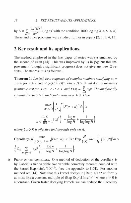
The method employed in the first paper of series was systematized by

the second of us in [14]. This was improved by us in [5]; but this im-

provement (though a significant progress) does not give any new Ω re-

sults. The net result is as follows.

Theorem 1. Let an be a sequence of complex numbers satisfying a1 =

1 and for n > 2, |an| < (n(H + 2))A, where H > 0 and A is an arbitrary

positive constant. Let 0 < H 6 T and F(s) =∞∑

n=1ann−s be analytically

continuable in σ > 0 and continuous in σ > 0. Then

max

σ > 0

1

H

∫

I

|F(σ + it)|2dt

>

CAΣ

n 6 H100+ 1|an|

2

(

1 −log n

log H+

1

log log H

)

where CA > 0 is effective and depends only on A.

Corollary. Ifmax

σ > 0, t in I|F(σ+it)| < Exp Exp

H

100, then

1

H

∫

I

|F(it)|2dt >

1

2CA

∑

n6 H100+1

|an|2

(

1 −log n

log H+

1

log log H

)

.

Proof of the corollary. One method of deduction of the corollary is16

by Gabriel’s two variable two variable convexity theorem coupled with

the kernel Exp .(sin(z/100)2), (see the appendix to [15]). For another

method see [14]. Note that this kernel decays in |Re z| 6 1/2 uniformly

at most like a constant multiple of (Exp Exp(c| Im z|))−1 where c > 0 is

a constant. Given faster decaying kernels we can deduce the Corollary

19

with more relaxed conditions. The same applies to all applications of

the key theorem. It may be remarked that we do not know any kernel

which decays (uniformly in |z| 6 1/2) at most like a constant multiple

of (Exp Exp(c| Im z|))−1 where c is any large positive constant.

We begin the applications by the following remark, which follows

from The theorem by putting F(s) = (ζ(α + s))k where α > 1/2 (we

may assume without loss of generality that H exceeds a large positive

constant) and k is a positive integer which may depend on H.

Theorem 2. We have, for α > 1/2,

max

σ > α, t in I|ζ(σ+it)| >

CA

∑

n6 H100

(dk(n))2

n2α

(

1 −log n

log H+

1

log log H

)

1/2k

,

where k 6 log H so that the condition dk(n) 6 (n(H+2))A is satisfied. (In

fact it may be noted that the maximum of RHS is attained in k 6 log H

itself).

Remark. We may also state a similar theorem for

max

σ > α, t ∈ I|ζ(σ + it)|−1

where α > 1/2 + δ and (σ > α − δ/2, t in I) is free from zeros of ζ(s).

Here δ is an arbitrary positive constant.

It is not very difficult to investigate the order of magnitude ofmax

k > 1

(R.H.S.) in Theorem 2. By a very ingenious argument, R. Balasubrama-

nian has shown (see [1]) that its logarithm is asymptotic to

C0(log H/ log log H)1/2

where C0 = 0.75 . . . , when α = 1/2. This gives the best known Ω result

max

σ > 12, t in I

|ζ(σ + it)| > Exp

[

34

(

log H

log log H

)1/2]

.

Earlier in [2], we had obtained a small positive constant in place of 17

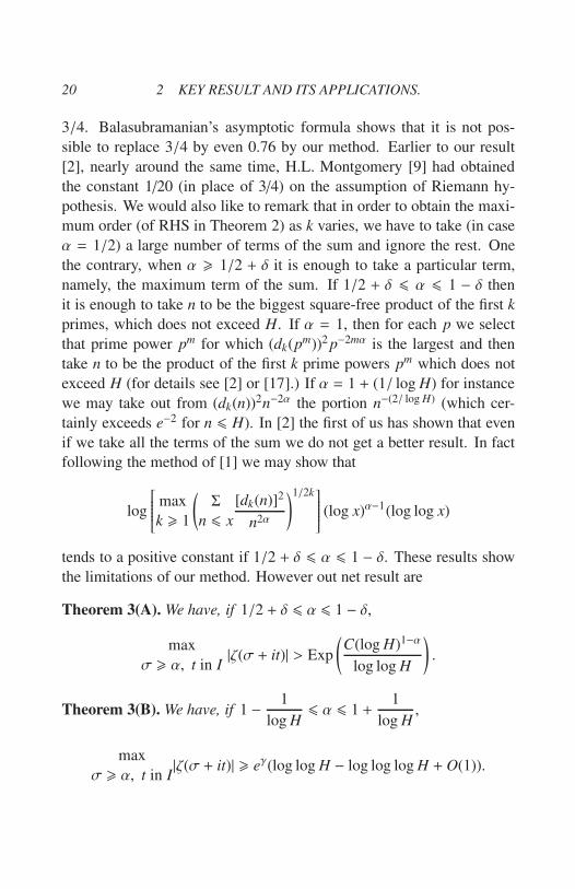
20 2 KEY RESULT AND ITS APPLICATIONS.

3/4. Balasubramanian’s asymptotic formula shows that it is not pos-

sible to replace 3/4 by even 0.76 by our method. Earlier to our result

[2], nearly around the same time, H.L. Montgomery [9] had obtained

the constant 1/20 (in place of 3/4) on the assumption of Riemann hy-

pothesis. We would also like to remark that in order to obtain the maxi-

mum order (of RHS in Theorem 2) as k varies, we have to take (in case

α = 1/2) a large number of terms of the sum and ignore the rest. One

the contrary, when α > 1/2 + δ it is enough to take a particular term,

namely, the maximum term of the sum. If 1/2 + δ 6 α 6 1 − δ then

it is enough to take n to be the biggest square-free product of the first k

primes, which does not exceed H. If α = 1, then for each p we select

that prime power pm for which (dk(pm))2 p−2mα is the largest and then

take n to be the product of the first k prime powers pm which does not

exceed H (for details see [2] or [17].) If α = 1 + (1/ log H) for instance

we may take out from (dk(n))2n−2α the portion n−(2/ log H) (which cer-

tainly exceeds e−2 for n 6 H). In [2] the first of us has shown that even

if we take all the terms of the sum we do not get a better result. In fact

following the method of [1] we may show that

log

max

k > 1

(

Σ

n 6 x

[dk(n)]2

n2α

)1/2k

(log x)α−1(log log x)

tends to a positive constant if 1/2 + δ 6 α 6 1 − δ. These results show

the limitations of our method. However out net result are

Theorem 3(A). We have, if 1/2 + δ 6 α 6 1 − δ,

max

σ > α, t in I|ζ(σ + it)| > Exp

(

C(log H)1−α

log log H

)

.

Theorem 3(B). We have, if 1 −1

log H6 α 6 1 +

1

log H,

max

σ > α, t in I|ζ(σ + it)| > eγ(log log H − log log log H + O(1)).

21

Remark 1. H. L. Montgomery [9] has shown that if 1/2+ δ 6 α 6 1− δ

then |ζ(a + it)| exceeds Exp[C(log t)1−α]/(log log t)α] for a sequence of

values of t tending to infinity by a different method. But this method

does not enable one to conclude that the maximum of |ζ(α+it)| as t varies

for example, over [T, 2T ] exceeds Exp[C(log T )1−α]/(log log T )α]. The

lower bound Exp[C(log T )1−α/(log log T )] given by our method seems

to be the best known till today.

Remark 2. N. Levinson [8] has shown by a different method that |ζ(1 + 18

it)| exceeds eγ log log t+O(1) for a sequence of values of t tending to in-

finity. But, for short intervals like [T, 2T ], ours is the only result known.

Remark 3. Let 1/2 + δ 6 α 6 1 − δ. I suspected that if we take F(s) =

(log ζ(α + s))k then we might get a better result Theorem 3(A). But it

was shown by H. L. Montgomery [10] that if (log ζ(s))k =∞∑

n=1

ak(n)n−s,

then

max

k > 1

∑

n6x

(ak(n))2n−2α

1/2k

lies between two constant multiples of (log x)1−α(log log x)−1.

Remark 4. H.L. Montgomery has conjectured [9] that if 1/2 6 α 6 1−δ

then |ζ(α + it)| does not exceed Exp([C(log t)1−α]/[log log t]α)

3 Further study of the maximum in 1/2 +δ 6 α 6

1 − δ by other methods.

In the second paper of the series [12], the second of us proved that if

1/2 + δ 6 α 6 1 − δ and I runs over all intervals, of fixed length H,

contained in [T, 2T ] then

log log

(

min

I

max

t in I|ζ(α + it)|

)

∼ (1 − α) log log H,

provided C < 100 log log T 6 H 6 Exp[D log T ]/[log log T ]) where C

is a large positive constant and D a positive constant depending only on

22 4 STUDY OF THE MAXIMUM ON σ = 1.

α. This aspect of the problem has been studied further by us in [2]. The

method is very closely related to a principle which we formulated and

employed in [6]. The main result of [3] is as follows:

Theorem 3. let α be as above, E > 1 an arbitrary constant, C 6 H 6

Exp

(

D log T

log log T

)

where C is a large positive constant and D an arbitrary

positive constant. Then there are > T H−E disjoint open intervals I (of

fixed length H) all contained in [T, 2T ], such that,

(log H)1−α

(log log H)α≪ max

t in I| log ζ(α + it)| ≪

(log log H)1−α

(log log H)α.

Here log ζ(s) is the analytic continuation in t > 2 along lines parallel to

the real axis (and free from zeros of ζ(s)) from σ > 1. The Vinogradov

symbol≪ means “less than a positive constant times”.

4 Study of the maximum on σ = 1.19

As a corollary to Theorem 3, we deduced in [4] the following

Theorem 4. Let J denote the interval I (of Theorem 3) with intervals of

length (log H)2 removed from both extremities. Then

max

t in J|ζ(1 + it)| 6 eγ[log log H + log log log H + O(1)].

Note that LHS is > eγ(log log H − log log log H +O(1)) by applying the

Corollary to the key theorem. (The conditions for deriving this lower

bound from the Corollary to the key theorem are satisfied in the course

of the proof of Theorem 3).

The key result of §2 can be used to obtain lower bounds for

max

σ > 1, t in I|ζ(σ + it)| and also a similar result (the lower bound gets

multiplied by the factor (6/π2) for |ζ(σ + it)|−1. But to obtain lower

23

bounds formax

t in I|ζ(1 + it)| and for

max

t in i|ζ(1 + it)|−1 we need conditions

looking like 100 log log log T 6 H 6 T . But by a somewhat compli-

cated application of the key result and other techniques the second of

us [13] proved the following theorem. To state the theorem it is bet-

ter to introduce some notation. The letter θ will, as before, denote the

least upper bound of the real parts of the zeros of ζ(s) (we do not know

whether θ < 1 or not). For x > 1 we define log1 x = log x and for

n > 2 we define logn x to be log(logn−1 x); similarly we define for real x,

Exp1(x) = Exp(x) and for n > 2 we define Expn(x) = Exp(Expn−1(x)).

Theorem 5. Consider for open intervals I (for t, of length H > 100)

contained in [T, 2T ] where T > T0, a large positive constant, the in-

equality

max

t in I|ζ(1 + it)| > eγ(log log H − log log log H − ρ), (∗)

where ρ is a certain real constant which is effective. Then we have the

following four results:

(1) (∗) holds for all I for which T > H > A1 log4 T

(2) If θ < 1 then (∗) holds for all I for which T > H > A2 log5 T.

(3) Let now H < A1 log4 T. Consider a set of disjoint intervals I (of

fixed length H) for which (∗) is false. Then the number of such

intervals I does not exceed T X−11

where X1 = Exp4(βH) where β

is a certain positive constant less than A−11

.

(4) Let now H < A2 log5 T. Consider a set of disjoint intervals I (of

fixed length H) for which (∗) is false. Then the number of such 20

intervals I does not exceed T X−12

where X2 = Exp5(β′H) where β′

is a certain positive constant which is less than A−12

.

5 An announcement

In this section the length of the interval will not be denoted by H. We

wish to announce a result [16] due to the second author which is ob-

24 REFERENCES

tained by quite a different method.

Theorem 6. Let ǫ be a constant satisfying 0 < ǫ < 1, T > T0(ǫ), a

constant depending only on ǫ, X = Exp

(

log T

log log T

)

. If from the inter-

vals T 6 t 6 T + eX we exclude certain (boundedly many depending

on ǫ) disjoint open intervals I each of length at most X−1, then in the

remaining portions of the interval, we have,

| log ζ(1 + it)| 6 ǫ log log T.

Further put β0 = A(log T )−mu(log log T )−2µ where µ = 2/3 and A is

any positive constant. Consider the rectangle R defined by σ > 1 − β0,

T 6 t 6 T + eX. Let I denote an open interval for t of length 1/X and let

J denote the corresponding rectangle σ > 1 − β0, t in I. Then with the

exception of certain boundedly many (depending on ǫ and A) disjoint

rectangles J we have for s in R,

| log ζ(s)| 6 ǫ log log T

where T > T0(ǫ, A)

Remark . The first result can be proved without assuming the Vino-

gradov’s zero free region. But if we assume the Vinogradov’s zero free

region, we get a better upper bound for the number of intervals which

have to be excluded. However, for the proof of the second part, the

Vinogradov zero free region is essential.

References

[1] R. Balasubramanian : On the frequency of Titchmarsh’s phe-

nomenon for ζ(s)-IV, Hardy-Ramanujan J., Vol. 9(1986), 1-10.

[2] R. Balasubramanian and K. Ramachandra : On the frequency of21

Titchmarsh’s phenomenon for ζ(s)-III, Proc. Indian Acad. Sci., 86

(A) (1977), 341-351.

REFERENCES 25

[3] R. Balasubramanian and K. Ramachandra : On the frequency of

Titchmarsh’s phenomenon for ζ(s)-V, Arkiv for Mathematik 26(1)

(1988), 13-20.

[4] R. Balasubramanian and K. Ramachandra : On the frequency of

Titchmarsh’s phenomenon for ζ(s)-VI, (to appear).

[5] R. Balasubramanian and K. Ramachandra : Progress towards a

conjecture on the mean-value of Titchmarsh series-III, Acta Arith.,

XLV (1986), 309-318.

[6] R. Balasubramanian and K. Ramachandra : On the zeros of a class

of generalised Dirichlet series-III, J. Indian Math. Soc., 41 (1977),

301-315.

[7] E. Bombieri and H. Iwaniec : On the order of ζ(1/2 + it), Ann.

Scoula Norm. Sup. Pisa. 13 no. 3 (1986), 449-472.

[8] N. Levinson : Ω theorems for the Riemann zeta-function, Acta

Arith, XX (1972), 319-332.

[9] H. L. Montgomery : Extreme values of the Riemann zeta-function,

Comment. Math. Helv., 52 (1977), 511-518.

[10] H. L. Montgomery : On a question of Ramachandra, Hardy-

Ramanunan J., 5 (1982), 31-36.

[11] K. Ramachandra : On the frequency of Titchmarsh’s phenomenon

for ζ(s)-I, J. London Math. Soc., (2) 8(1974), 683-690.

[12] K. Ramachandra : On the frequency of Titchmarsh’s phenomenon

for ζ(s)-II, Acta Math. Acad. Sci. Hungaricae, Tomus 30 (1-2),

(1977), 7-13.

[13] K. Ramachandra : On the frequency of Titchmarsh’s phenomenon

for ζ(s)-VII, (to appear).

[14] K. Ramachandra : Progress towards a conjecture on the mean-

value of Titchmarsh series-I, Recent Progress in Analytic Number

26 REFERENCES

Theory (Edited by H. Halberstam and C. Hooley) Vol. I, Academic

Press (1981), 303-318.

[15] K. Ramachandra : A brief summary of some results in the ana-22

lytic theory of numbers-II Addendum, Number Theory. Proceed-

ings, Mysore (1981), Edited by K. Alladi, Lecture Notes in Math-

ematics, 938, Springer Verlag, 106-122.

[16] K. Ramachandra : A remark on ζ(1+ it), Hardy-Ramanujan J., 10

(1987) (to appear).

[17] K. Ramachandra and A. Sankaranarayanan : Omega theorems for

the Hurwitz zeta-function, (to appear).

[18] H. E. Richert : Zur Abschatzung der Riemannschen Zetafunktion

in der Nahe der Verticalen σ = 1, Math. Ann., 169 (1967), 97-101.

[19] E. C. Titchmarsh : The theory of the Riemann zeta-function,

Clarendon Press, Oxford (1951).

[20] A. Walfisz : Weylsche exponential Summen in der neueren Zahlen-

theorie, VEB Deutscher Verlag der Wiss., Berlin (1963) .

* Institute of Mathematical Sciences

Madras - 600 113, Tamil Nadu

India

** School of Mathematics

Tata Institute of Fundamental Research

Homi Bhabha Road

Bombay-400 005

India

RAMANUJAN’S FORMULAS FOR

EISENSTEIN SERIES

By Bruce C. Berndt*

As is customary, N denotes the set of positive integers, Z denotes the 23

ring of rational integers, H = τ : Im τ > 0, and

Γ0(n) =

(

a b

c d

)

: a, b, c, d ∈ Z, ad − bc = 1, c ≡ 0(mod n)

,

where n ∈ N. If n = 1, Γ0(1) is the full modular group Γ(1).

Let

E2(τ) = 1 − 24

∞∑

k=1

kq2k

1 − q2k

and

Fn(τ) = E2(τ) − nE2(nτ),

where q = eπiτ, τ ∈ H , and n ∈ N. Although E2(τ) is not a modular

form, it can be easily shown that Fn(τ) is a modular form of weight 2

and trivial multiplier system on Γ0(n).

In a very famous paper [8, pp. 23-39], Ramanujan gave formu-

las for Fn when n = 2, 3, 4, 5, 7, 11, 15, 17, 19, 23, 31, 35. However, no

proofs are indicated. Furthermore, in Chapter 21 of his second note-

book [9], Ramanujan offers, without proofs, formulas for Fn when n =

3, 5, 7, 9, 11, 15, 17, 19, 23, 25, 31, 35. In contrast to [8] where only one

formula is given for each value of n, in [9] several formulas are stated

for most values of n.

*Research partially supported by a grant from the Vaughn Foundation.

27

28

Part of Ramanujan’s motivation in calculating Fn arose from its ap-

pearance in certain approximations to π found by Ramanujan [8]. J.M.

and P.B. Borwein [6] have extensively developed Ramanujan’s ideas.

Using their work, we shall very briefly indicate how these approxima-

tions are obtained. Let K denote the complete elliptic integral of the

first kind associated with the modulus k, where 0 < k < 1, and let E′

denote the complete elliptic integral of the second kind associated with

the complementary modulus k′ =√

1 − k2. For r > 0, define

α(r) =E′

K−

π

4K2,

where k = k(r) = θ22(e−π

√r)/θ2

3(e−π

√r), where θ2 and θ3 are the classical24

theta-functions, usually so denoted. Put αm = α(n2mr), where m ∈ N ∪0 and n ∈ N. There exists a recursion formula for αm in terms of Fn

[6, p. 158]. This leads to an approximation of for 1/π given by

0 < αm − 1/π < 16nm√

re−nm√

rπ

provided that rn2m> 1 [6, p. 169]. For complete details, see [6].

The Borweins leave the calculation of Fn for n = 2, 3, 4 as exercises

[6, p. 161]. In fact, they [6, 9. 158] state that “The verification... is

tedious but straightforward for small n. For larger n, we rely on Ra-

manujan.” The Surpose of this paper is to indicate how Ramanujan’s

formulas for Fn can be proved. Complete proofs for all of Ramanu-

jan’s formulas for Fn can be found in the author’s forthcoming book [2].

We offer two general approaches. The first is probably similar to that

employed by Ramanujan, while the second depends upon the theory of

modular forms.

The first method rests upon modular equations. Thus, we need to

give the definition of a modular equation, as understood by Ramanujan.

Definition . Let K, K′, L, and L′ denote complete elliptic integrals of

the first kind associated with the moduli k, K′, l, and l′, respectively.

Suppose that the equality

nK′

K=

L′

L(1)

RAMANUJAN’S FORMULAS FOR EISENSTEIN SERIES 29

holds for some n ∈ N. Then a modular equation of degree n is a relation

between the moduli k and l which is implied by (1).

Ramanujan sets α = k2 and β = l2.

If q = exp(−πK′/K) and

ϕ(q) =

∞∑

j=−∞q j2

then it is well known that

K =π

2ϕ2(q).

Furthermore, set zn = ϕ2(qn).

Definition . The multiplier m for a modular equation of degree n is de-

fined by

m =K

L=ϕ2(q)

ϕ2(qn)=

z1

zn

.

In his notebooks [9], Ramanujan devotes more space to modular 25

equations than to any other topic. Despite this, Ramanujan never pub-

lished any of his work on modular equations, except for the aforemen-

tioned formulas for Eisenstein series in [8]. For an expository account

of Ramanujan’s discoveries on modular equations, see our paper [1].

Some of Ramanujan’s modular equations have been proved in three pa-

pers [3], [4], [5] that we have coauthored with A. J. Biagioli and J. M.

Purtilo. For proofs of all of Ramanujan’s modular equations, see the

author’s forthcoming book [2].

We now state perhaps the primary formula that Ramanujan em-

ployed in establishing formulas for Fn(τ). He has not stated this for-

mula in either [8] or [9]. However, some cryptic remarks on p. 253 of

his second notebook [9] point to a result such as that given below.

Theorem 1. Let q, Fn, α, β, m, and z1 be as given above. Then

Fn(τ) = −α(1 − α)z21

d

dαLog

(

β(1 − β)

m6α(1 − α)

)

.

30

We now sketch proofs for three of seven formulas for F3(τ) found

in Entry 3 of Chapter 21 in Ramanujan’s second notebook [9].

Theorem 2. Let ϕ, α, and β be as given above. Put

ψ(q) =

∞∑

j=0

q j( j+1)/2.

Then

S 3(τ) : = −1

2F3(τ) =

ϕ4(q) + 3ϕ4(q3)

4ϕ(q)ϕ(q3)

2

(2)

= ϕ2(q)ϕ2(q3) − 4qψ2(−q)ψ2(−q3) (3)

=1

2ϕ2(q)ϕ2(q3)

1 +√

αβ +√

(1 − α)(1 − β)

. (4)

The last formula was stated by Ramanujan in [8], [10, p. 33].

Proof. Letting n = 3 in Theorem 1, we find that

S 3(τ) =1

2α(1 − α)z2

1

d

dαLog

(

β(1 − β)

m6α(1 − α)

)

. (5)

We need to determine the interdependence of α, β and m in order to

calculate the derivative above. From our work [2] on modular equations

of degree 3 in Section 5 of Chapter 19 in Ramanujan’s second notebook

[9],

α(1 − α) =(m2 − 1)(9 − m2)3

256m6, (6)

β(1 − β)

α(1 − α)=

m4(m2 − 1)2

(9 − m2)2, (7)

and26

dm

dα=

16m4

(9 − m2)2. (8)

RAMANUJAN’S FORMULAS FOR EISENSTEIN SERIES 31

Substituting (6)-(8) into (5) and employing the chain rule, we deduce

that

S 3(τ) =(m2 − 1)(9 − m2)

16m2z2

1

d

dmLog

(

m2 − 1

m(9 − m2)

)

(9)

=z2

1

16m3(m2+ 3)2.

If we now use the definition of m, we find that (2) readily follows.

Using again the definition of m, we may rewrite (9) in the form

S 3(τ) = z1z3

(

1 − (9 − m2)(m2 − 1)

16m2

)

(10)

= z1z3(1 − αβ(1 − α)(1 − β)1/4),

where we have employed (6) and (7). Now in Chapter 17 of his second

notebook [9], Ramanujan offers a “catalogue” of evaluations of theta-

functions in terms of q(qn), α(β), and z1(zn). In particular, from Entry

11,

ψ(−q) = (1

2z1)1/2α(1 − α)/q1/8

and

ψ(−q3) = (1

2z3)1/2β(1 − β)/q31/8.

Solving these two equalities for α(1 − α) and β(1 − β), respectively, and

substituting them in (10), we immediately deduce (3).

The simplest modular equation of degree 3 is given by

(αβ)1/4+ (1 − α)(1 − β)1/4 = 1. (11)

This was first discovered by Legendre and may be found in Cayley’s

book [7, p. 196], for example. Ramanujan [9, chpater 19, Entry 5(ii)]

rediscovered (11). If we square both sides of (11) and substitute in (10),

we immediately deduce (4).

Unfortunately, we have been unsuccessful in using Theorem 1 to

establish certain formulas of Ramanujan for Fn(τ). We thus have had

32

to invoke the theory of modular forms in these cases. In order to offer 27

one such example, we need to make an additional definition. Let, in the

notation of Ramanujan,

f (−q) =

∞∏

j=1

(1 − q j),

where, as above, q = eπiτ. Note that f (−q2) = q−1/12η(τ), where η

denotes the Dedekind eta-function. We now state Entry 8(i) in Chapter

21 of Ramanujan’s second notebook [9].

Theorem 3. Let ϕ, ψ, and f be defined as above. Then

−1

2F11(τ) = 5ϕ2(q)ϕ2(q11) − 20q f 2(q) f 2(q11) (12)

+ 32q2 f 2(−q2) f 2(−q22) − 20q3ψ2(−q)ψ2(−q11).

We now briefly describe how the theory of modular forms can be

used to prove Theorem 3. The functions ϕ(q), ψ(q), and f (−q) are asso-

ciated with modular forms of weight 1/2 on

Γ(2) = (

a b

c d

)

∈ Γ(1) : a ≡ d ≡ 1(mod 2), b ≡ c ≡ 0(mod 2).

Thus, (12) is first converted into an equality relating modular forms.

Each of the five expressions in (12) is a modular form of weight 2 on

Γ(2) ∩ Γ0(11). We have already mentioned that the multiplier system

of F11(τ) is trivial. By employing the multiplier system of η(τ), we can

show that each of the four expressions on the right side of (12) also has

a trivial multiplier system.

Let Γ = Γ(2) ∩ Γ0(p), where p is an odd prime. Let F be a funda-

mental set for Γ. If F is a nonconstant modular form of weight r on Γ,

then the valence formula

∑

z∈FOrdΓ(F; z) =

1

2r(p + 1) (13)

REFERENCES 33

is valid, where OrdΓ(F : z) is the invariant order of F at z. Suppose that

we can show that the coefficients of q0, q1, q2, . . . , qµ in F are equal to

0, i.e. OrdΓ(F;∞) > µ + 1. Suppose furthermore that µ+ 1 > 12r(p + 1).

Then if OrdΓ(F : z) > 0 for each z ∈ F ,

∑

z∈FOrdΓ(F; z) > OrdΓ(F;∞) > µ + 1 >

1

2r(p + 1).

Hence F(τ) ≡ 0, for otherwise, we could have a contradiction to the

valence formula (13).

Now write the proposed identity (12) in the form 28

F := F1 + . . . + F5 = 0. (14)

We have shown that F is a modular form of weight 2 and trivial multi-

plier system on Γ = Γ(2) ∩ Γ0(11). Moreover, OrdΓ(F : z) > 0 for each

z ∈ F . Since (1/2)r(p + q) = 12, it suffices to show that the coeffi-

cients of q j, 0 6 j 6 12, in F are equal to 0 in order to prove (14), and

hence also (12). Using MACSYMA, we have indeed done this, and so

the proof of Theorem (3) has been completed.

More complete details on the use of modular forms and MACSYMA

in proving modular equations may be found in [2] and [4].

We are grateful to A.J. Biagioli and J.M. Purtilo for their collabora-

tion on modular forms and MACSYMA, respectively.

References

[1] B.C. Berndt : Ramanujan’s modular equations, Ramanujan Revis-

ited, Academic Press, Boston 1988, 313-333.

[2] B.C. Berndt : Ramanujan’s Notebooks, Part III, Springer Verlag,

New York, to appear.

[3] B.C. Berndt, A.J. Biagioli and J.M. Purtilo : Ramanujan’s

“mixed” modular equations, J. Ramanujan Math. Soc. 1(1986),

46-70.

34 REFERENCES

[4] B.C. Berndt, A.J. Biagioli, and J.M. Purtilo : Ramanujan’s mod-

ular equations of “large” prime degree, J. Indian Math. Soc., 51

(1987), 75-110.

[5] B.C. Berndt, A.J. Biagioli, and J.M. Purtilo : Ramanujan’s mod-

ular equations of degrees 7 and 11, Indian J. Math., 29 (1987).

215-228.

[6] J.M. and P.B. Borwein : Pi and the AGM, John Wiley, New York,

1987.

[7] A. Cayley : An Elementary Treatise on Elliptic Functions, Second

Ed., Dover, New York, 1961.

[8] S. Ramanujan : Modular equations and approximations to π,29

Quart. J. Math. 45(1914), 350-372.

[9] S. Ramanujan : Notebooks (2 Volumes), Tata Institute of Funda-

mental Research, Bombay, 1957.

[10] S. Ramanujan : Collected Papers, Chelsea, New York, 1962.

Departement of Mathematics

University of Illinois

1409 West Green street

Urbana, Illinois 61801

U.S.A.

ON THE PROOF OF ANDREWS’

q-DYSON CONJECTURE

By D. M. Bressoud*

This is a breif sketch of work done by Doron Zeilberger, Ian Goulden 31

and myself in late 1983 and early 1984 which settled in the affirmative

a conjecture made by George Andrews [1] as well as more detailed con-

jectures made by Kevin Kadell [12].

The problem has its origins in the evaluation of a definite integral

which arose in a physical problem [5], its solution has given evaluations

for other definite integrals arising in physics [4]. The original integral

was discovered by Freeman Dyson [5]:

I(n, z) = (2π)−n

2π∫

0

. . .

2π∫

0

|∆n(eiθ)|2zdθ1 . . . dθn, (1)

where

∆n(eiθ) = Π(eiθ j − eiθk ), 1 6 j < k 6 n.

Dyson conjectured that

I(n, z) =Γ(nz + 1)

Γn(z + 1), (2)

a conjecture which was simultaneously and independently proved by

Gunson [7] and Wilson [23].

It is sufficient to prove that conjecture for positive integral integral

z. In this case, we can use the following equality:

|∆n(eiθ)|2 = Π(eiθ j − eiθk )(e−iθ j − e−iθk ). (3)

*Partially supported by N.S.F. grant no. DMS.-8521580

35

36

= Π(1 − ei(θ j−θk))(1 − ei(θk−θ j)).

If we set x j = eiθ j , then the integral picks out the constant term in a

polynomial in x1, x−11, . . . , xn, x

−1n . Given a monomial, M, in the xi’s, let

[M] denote the coefficient of M in the succeeding polynomial. Let x0

denote the monomial in which each xi appears to the power 0. Equation

(2) for z ∈ N can be restated as

[x0]Π(1 − x j/xk)z(1 − xk/x j)z=

(nz)!

(z!)n, 1 6 j < k 6 n. (4)

32

Dyson discovered that more was probably true, and actually stated

his conjecture in the following form:

[x0]Π(1 − x j/xk)ak (1 − xk/x j)a j (5)

=(a1 + . . . + an)

a1! . . . an!

In 1975, Andrews [1] noted that equation (5) seemed to have a nice

generalization in which the product (1 − x)a could be replaced by

(x)a = (1 − x)(1 − xq)(1 − xq2) . . . (1 − xqa−1)

Specifically, Andrews conjectured the following:

[x0]Π(x j/xk)ak(qxk/x j)a j

, 1 6 j < k 6 n, (6)

=(q)a1+...+an

(q)a1. . . (q)qn

.

On reason for the interest in equations (5) and (6) is the intractabil-

ity of the blunt approach. If one expands the binomials in equations

(5), the constant term is a simple summation when n = 3, and Dyson’s

conjecture is the classical identity:

∑

i

(−1)i

(

a1 + a2

i

) (

a2 + a3

i − a2 + a3

) (

a1 + a3

i + a1 − a2

)

(7)

ON THE PROOF OF ANDREWS’ q-DYSON CONJECTURE 37

= (−1)a2

(

a1 + a2 + a3

a1, a2, a3

)

.

For larger n, however, the constant term is an(

n−12

)

-fold summation,

and virtually nothing is known about such non-trivial multiple summa-

tions.

The same situation applies to Andrews’ conjecture, except that in-

stead of multiple hypergeometric series we get multiple basic hyperge-

ometric series.

To understand how equation (6) was first proved, one must under-

stand an ingenious combinatorial proof of Dyson’s equation (5) which

was found by Zeilberger [24] a few years earlier. Equation (5) is equiv-

alent to

[(xa1

1. . . x

ann )n−1]Π(x j − xk)a j+ak (8)

= (−1)a2+2a3+...+(n−1)an(a1 + . . . + an)!

a1! . . . an!.

We can formally expand the product of binomials in equation (8): 33

Π(x j − xk)a j+ak =

∑

T∈T ∗

(−1)u(T ) xw1(T )

1. . . x

wn(T )n (9)

where T ∗ is the set of “multi-tournaments” in which each pair of play-

ers, say j and k, meet a total of a j + ak times and the “winner” of each

game is recorded. The exponent wi(T ) is the number of games won by

player i, and u(T ) records the number of “upsets” : k > j and k beats j.

If we let T ⊆ T ∗ be the subset of multi-tournaments in which each

player j wins (n − 1)a j games, then equation (8) can be restated as:

∑

T∈T

(−1)u(T )= (−1)a2+...+(n−1)an

(

a1 + . . . + an

a1, . . . , an

)

. (10)

The right side of equation (10) involves the multinomial coefficient

which counts the number of “words” which can be constructed with

a11′s, a22’ s, . . . , ann′s. Each such word corresponds to a multi-tourna-

ment in a natural way. Given j and k, remove the subword of length

38

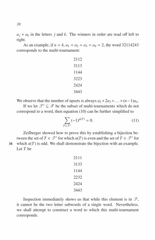
a j + ak in the letters j and k. The winners in order are read off left to

right.

As an example, if n = 4, a1 = a2 = a3 = a4 = 2, the word 32114243

corresponds to the multi-tournament:

2112

3113

1144

3223

2424

3443

We observe that the number of upsets is always a2+2a3+ . . .+ (n−1)an.

If we let T ′ ⊆ F be the subset of multi-tournaments which do not

correspond to a word, then equation (10) can be further simplified to∑

T∈T ′

(−1)µ(T )= 0. (11)

Zeilberger showed how to prove this by establishing a bijection be-

tween the set of T ∈ T ′ for which u(T ) is even and the set of T ∈ T ′ for

which u(T ) is odd. We shall demonstrate the bijection with an example.34

Let T be

2111

3133

1144

2232

2424

3443

Inspection immediately shows us that while this element is in T ,

it cannot be the two letter subwords of a single word. Nevertheless,

we shall attempt to construct a word to which this multi-tournament

corresponds.

ON THE PROOF OF ANDREWS’ q-DYSON CONJECTURE 39

The leading entries of each row define a tournement:

2 beats 1, 3 beats 1, 1 beats 4, etc. Schematically, this tournament is

given by:

1

4

2

GG

@@// 3

WW

^^

We call a tournament “transitive” if it contains no cycles, “non-transi-

tive” otherwise. If our multi-tournament arose from a single word, then

this tournament is transitive and the player beating everyone else is the

first letter of the word. Since our tournament is transitive, it is possible

at this stage that it comes from a single word. We record the first letter

: 2, and modify the tournement by looking at the next outcome of the

games of player 2: 1 beats 2, 2 beats 3, 4 beats 2.

The tournament becomes :

1

4

2 // 3

WW

^^

Our tournament is now non-transitive which will eventually happen

if and only if T is in T ′.

Every non-transitive tournament contains a 3-cycle and reversing

the arrows in a 3-cycle will change the parity of the number of upsets

in the tournament. We have two 3-cycles in this tournament. which one

we choose to reverse is significant. 35

If we reverse 2 → 3 → 4 → 2 and then restore the first letter, 2, we

get the multi-tournament

2111

40

3133

1144

2332

2224

4443

But the leading entries of this multi-tournament give us a non-transitive

tournament:

1

4

2

GG

@@// 3

WW

An iteration of our procedure would not take us back to the original

multitournament.

If no letters of the word have been recorded, then it doesn’t matter

which 3-cycle we reverse as long as we are consistent. If at least one

letter has been recorded, then we are in a peculiar situation. Let v1 be the

last letter recorded. Since we have only changed the arrows connected

to v1, all cycles of the non-transitive tournament include vertex v1.

Let the remaining vertices be labelled v2, v3, . . . , vn where v2 beats

v3 beats . . . beats vn, and choose the smallest i for which v1 beats vi and

vi+1 beats v1. It is the 3-cycle v1 → vi → vi+1 → v1 that we reverse.

it is exactly this procedure that was used to prove Andrews’ conjec-

ture, except that the details are more complicated because the parameter

q introduces an additional weight on the multi-tournaments.

The proof first demonstrates that

[x0]Π(x j/xk)ak(qxk/x j)a j

(12)

= (−1)a2+...+(n−1)an

∑

t∈F

(−1)µ(T )qwt(T ), (13)

where wt(T ) is the sum of the “Major Indices” of all the two letter words

in the multi-tournament. The Major Index of a word is the sum of the

ON THE PROOF OF ANDREWS’ q-DYSON CONJECTURE 41

number of letters to the left of each “descent” in the word. Thus 36

32114243

has four descents : (32, 21, 42, 43) , and its major index is 1+2+5+7 =

15.

On the other hand, if we sum the major indices of the two letter

subwords of 32114243, we get 1 + 1 + 0 + 1 + 2 + 3 = 8. This sum

of Major Indices is called the Z-statistic, denoted Z(T ). The second

part of the proof involves showing that the sum of qZ(T ) over all multi-

tournaments corresponding to a single word is equal to

(q)a1+...+an

(q)a1. . . (q)an

Equation (6) now reduces to verifying that∑

T∈T ′

(−1)u(T )qwt(T )= 0. (14)

The bijection given above does not preserve weights. The last and most

elaborate part of the proof involves finding and verifying a bijection

which does.

It is curious that this combinatorial approach is still the only known

proof of equation (6).

Goulden and I[3] generalized this proof of yield a more useful iden-

tity. In the following we let A be an arbitrary set of unordered pairs

( j, k), 1 6 j , k 6 n, χ(S ) is 1 if S is true, 0 otherwise, SA is the set of

permutations of 1, . . . , n for which j > i and σ−1(i) implies (i, j) < A,

and wt(σ) is the sum over all j of a j times the number of k < j for which

σ−1( j) < σ−1(k).

[x0]Π(x j/xk)a j(qxk/x j)ak−χ(( j,k)∈A) (15)

=(q)a1+...+an

(q)a1. . . (q)an

∑

σ∈SA

qwt(σ)Π j

1 − qaσ( j)

1 − qaσ(1)+...+aσ( j)(16)

This identity implies several conjectures of Kadell [12] and has had

applications in studying the characters of S L(n,C)[21] and in evaluating

definite integrals arising in statistical mechanics [4].

42 REFERENCES

The theorems first conjectured by Dyson and Andrews are only the

tip of the iceberg of a very extensive theory. These identities are related

to the Vandermonde determinant formula which is Weyl’s denominator

formula for the root system An. Macdonald [15] conjectured the appro-

priate generalizations to arbitrary root systems and he and W.G. Morris37

[16] gave conjectures and some proofs for the basic analogs.

Macdonald’s conjecture for the root system BCn was discovered to

be equivalent to a multi-dimensional beta integral evaluation of Selberg

[18, 19]. A basic analog of this was conjectured by Askey [2]. Habsieger

[8] and Kadell [13] independently proved Askey’s conjecture and then

Habsieger [9] and Zeilberger [25] showed that this integral evaluation

implied some of Morris’ conjectures.

Most recently, Kadell [14] has proved Macdonal’s conjecture for the

basic analog of the BCn conjecture, Garvan [6] has done the same for

F4, and E.M. Opdam [17] has proved the original Macdonald conjecture

for arbitrary root systems. Only the basic analogs for the special root

systems E6, E7 and E8 are unproven at the moment.

Stembridge [22] has found a strikingly simple proof of Andrews’

conjecture in the case where the parameters are equal. He has also found

formulas for some of the non-constant terms [21]. Connections with rep-

resentation theory can be found in an article by Stanley [20]. Hanlon has

pursued the connections between these identities and cyclic homology

[10, 11].

References

[1] G. E. Andrews : Problems and prospects for basic hypergeometric

functions, in Theory and Application of Special Functions, ed. R.

Askey, Academic Press, New York, 1975, 191-224.

[2] R. A. Askey : Some basic hypergeometric extensions of integrals

of Selberg and Andrews, SIAM J. Math. Anal. 11 (1980), 938-951.

[3] D. M. Bressoud and I. P. Goulden : Constant term identities

extending the q-Dyson Theorem, Trans. Amer. Math. Soc. 291

REFERENCES 43

(1985), 203-228.

[4] D. M. Bressoud and I. P. Goulden : The generalized plasma in 38

one dimension : evaluation of a partition function, Commun. Math.

Phys. 110(1987), 287-291.

[5] F. J. Dyson : Statistical theory of the energy levels of complex

systems, J. Math. Physics 3(1962), 140-156.

[6] F. Garvan : Personal communication.

[7] J. Gunson : Proof of a conjecture by Dyson in the statistical theory

of energy levels, J. Math. Physics 3 (1962) , 752-753.

[8] L. Habsieger : Une q-integrale de Selberg-Askey, SIAM J. Math,

Anal., to appear.

[9] L. Habsieger : La q-conjecture de Macdonald-Morris pour G2, C.

R. Acad. Sc. Paris 302 (1986), 615-618.

[10] P. Hanlon : The proof of a limiting case of Macdonald’s root sys-

tem conjecture, Proc. London Math. Soc. 49 (1984), 170-182.

[11] P. Hanlon : Cyclic homology and the Macdonald conjectures, In-

vent. Math. 86 (1986), 131-159.

[12] K. Kadell : Andrews’ q-Dyson conjecture : n = 4, Trans. Amer.

Math. Soc. 290 (1985), 127-144.

[13] K. Kadell : A proof of Askey’s conjectured q-analog of Selberg’s

integral and a conjecture of Morris, SIAM J. Math. Anal., to appear.

[14] K. Kadell : Personal communication.

[15] I. G. Macdonald : Some conjectures for root systems. SIAM J.

Math. Anal. 13 (1982), 988-1007.

[16] W. G. Morris : Constant term identities for finite and infinite root

systems, Ph. D. thesis, University of Wisconsin, Madison, 1982.

44 REFERENCES

[17] E. M. Opdam : Doctoral thesis, University of Leiden, Netherlands.

[18] A. Selberg : Uber einen Satz von A. Gelfond, Arch. Math.

Naturvid. 44 (1941), 159-170.

[19] A. Selberg : Bemerkninger om et multiplelt integral, Norsk Mat.

Tidsskr. 26, (1944), 71-78.

[20] R. Stanley : The q-Dyson conjecture, generalized exponents and39

the internal product of Schur functions, in “Combinatorics and

Algebra” ed. Curtis Greene, Amer. Math. Soc., Providence, 1984,

81-94.

[21] J. Stembridge : First layer formula for the characters of S L(n,C),

Trans, Amer. Math. Soc. 299 (1987), 319-350.

[22] J. Stembridge : A short proof of Macdonald’s conjecture for the

root systems of type A. Preprint.

[23] K. Wilson : Proof of a conjecture by Dyson, J. Math. Physics 3

(1962) 1040-1043.

[24] D. Zeilberger : A combinatorial proof of Dyson’s conjecture, Dis-

crete Math. 41 (1982), 988-1007.

[25] D. Zeilberger : A proof of the G2 case of Macdonald’s root system

– Dyson conjecture, SIAM J. Math Anal. 18 (1987), 880-883.

[26] D. Zeilberger and D. Bressoud : A proof of Andrews’ q-Dyson

conjecture, Discrete Math. 54 (1985), 201-224.

Penn State University,

University Park, PA 16802

WEYL’S INEQUALITY, WARING’S

PROBLEM AND DIOPHANTINE

APPROXIMATION

By D. R. Heath-Brown

For fixed positive integers s and k, we define 41

Rs,k(N) = #(n1, . . . , n2) ∈ Ns :

s∑1

nkj = N

One central question in Waring’s problem is to prove the Hardy-

Littlewood asymptotic formula

Rs,k(N) =Γ(1 + 1/k)s

Γ(s/k)S(N)N(s/k)−1

+ O(N(s/k)−1−δ) (1)

for as large a range of s as possible. To tackle this, one uses an expo-

nential sum

S (α) =

P∑n=1

e(αnk),

where P = [N1/k]. One then has

Rs,k(N) =

1∫

0

S (α)se(−αN)dx. (2)

The trivial bound for S (α) is |S (α)| 6 P. However, one can improve

on this for suitable α, by using the following estimate.

45

46

Weyl’s inequality. Let |α − a/q| 6 q−2, with (a, q) = 1. Then

S (α) ≪ǫ P1+ǫ (q−1+ P−1

+ qP−k)21−k

,

for any ǫ > 0.

Thus if α can be approximated with P 6 q 6 Pk−1 one has

S (α)≪ P1−21−k+ǫ , (3)

and the corresponding contribution to (2) is

≪ Ps(1−21−k+ǫ) ≪ N s/k−1−δ ,

provided that s > 2k−1k. Those α which have no useable approximation

produce the main term of (1). Thus one obtains (1) for s > 1 + 2k−1k.

One can improve on this agrument by using an average bound.42

Hua’s inequality. For any ǫ > 0, one has

1∫

0

|S (α)|2k

dα ≪ǫ P2k−k+ǫ .

This leads to (1) for s > 1 + 2k. Until recently, this was the best

known range for (1), for small k > 3.

The sum S (α) may also be used in Diophantine approximation prob-

lems. It was shown by Danicic [2] that if ǫ > 0 and k ∈ N are given,

then there exists P(ǫ, k) as follows. For any P > P(ǫ, k) and any α ∈ R,

one can find n 6 P with

||αnk || 6 Pǫ−21−k

. (4)

This generalizes Dirichlet’s approximation Theorem, when k = 1,

and a result of Heilbronn (4), for k = 2. To prove Danicic’s theorem

one can use a result of Montgomery (see Baker [1, Theorem 2.2]): If

||an || > ∆ for 1 6 n 6 P, then∑

16h6∆−1

|∑n6P

e(han)| > P/6.

WEYL’S INEQUALITY, WARING’S PROBLEM AND DIOPHANTINE

APPROXIMATION 47

We therefore wish to estimate

∑h6∆−1

|S (αh)|. (5)

As with Weyl’s inequality, this can be done satisfactorily, with a

relative saving of P−21−k+ǫ , unless α has an approximation

|α − a/q| 6∆

qPk−1, q 6 P. (6)

Thus Montgomery’s result allows us to take ∆ ≈ Pǫ−21−k

. Of course,

if (6) holds then ||αqk || 6 ∆, and q 6 P.

A sharpening of Weyl’s inequality has recently been obtained (Heath-

Brown [3]).

Theorem 1. Let |α− a/q| 6 q−2 with (a, q) = 1, and suppose that k > 6.

Then

S (α)≪ǫ P1+ǫ(Pq−1+ P−2

+ qP1−k)(4+3)2−k

for any ǫ > 0.

Thus 43

S (α)≪ P1−(4/3)21−k+ǫ ,

if P36 q 6 Pk−3. One therefore has a sharper bound than (3), but for a

shorter range of q, (and only for k > 6). Closely related to Theorem 1 is

an improvement on Hua’s Inequality (Heath-Brown [3]).

Theorem 2. Let k > 6 and ǫ > 0. Then

1∫

0

|S (α)|(7/8)2k

dα ≪ P(7/8)2k−k+ǫ .

As before one may deduce :

Corollary. The Hardy-Littlewood asymptotic formula [1] holds for k >

6 and s > 1 +7

82k.

48

One may also try to sharpen Danicic’s result. One obtains a saving

in (5) of

P−(4/3)21−k+ǫ

relative to the trivial estimate, unless

|α − a/q| 6∆

qPk−3, q 6 P3.

Unfortunately in this latter case, one gets no useable bound for ||aqk ||.

The attempt to improve on (4) therefore fails. However, if one starts with

an approximation |α − a/q| 6 q−2 and fixes P = [q(1/3)], for example,

one is led to an “unlocalized” result (Heath-Brown [3]).

Theorem 3. Let α ∈ R and ǫ > 0 be given. For any integer k > 6, there

are infinitely many n ∈ N with

||αnk || 6 nǫ−(4/3)21−k .

Let us now look at the proof of Theorem 1. One uses Weyl’s “square

and difference” trick, but with the symmetric difference

(∇h)(x) = (x + h) − (x − h)

in place of the forward difference. After j steps, one has

|S (α)|2j

≪ P2 j− j−1∑

h1,...,h j

|R(α)|, (7)

where |hi| < P/2 and44

R(α) = R(α; h1, . . . , h j) =∑n∈I

e(α∇h1. . .∇h j

(nk)).

Here I is a subinterval of [1, P], depending on h1, . . . , h j. As a func-

tion of n, the polynomial

∇h1. . .∇h j

(nk)

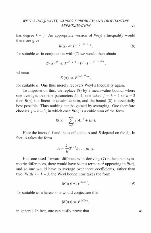
WEYL’S INEQUALITY, WARING’S PROBLEM AND DIOPHANTINE

APPROXIMATION 49

has degree k − j. An appropriate version of Weyl’s Inequality would

therefore give

R(α)≪ P1−21−(k− j)+ǫ , (8)

for suitable α. in conjunction with (7) we would then obtain

|S (α)|2j

≪ P2 j− j−1 · P j · P1−21−(k− j)+ǫ

,

whence

S (α)≪ P1−21−k+ǫ ,

for suitable α. One thus merely recovers Weyl’s Inequality again.

To improve on this, we replace (8) by a mean-value bound, where

one averages over the parameters hi. If one takes j = k − 1 or k − 2

then R(α) is a linear or quadratic sum, and the bound (8) is essentially

best possible. Thus nothing can be gained by averaging. One therefore

chooses j = k − 3, in which case R(α) is a cubic sum of the form

R(α) =∑n∈1

e(An3+ Bn).

Here the interval I and the coefficients A and B depend on the hi. In

fact, A takes the form

A =k!

62k−3h1 . . . hk−3.

Had one used forward differences in deriving (7) rather than sym-

metric differences, there would have been a term in n2 appearing in R(α),

and so one would have to average over three coefficients, rather than

two. With j = k − 3, the Weyl bound now takes the form

|R(α)| ≪ P3/4+ǫ , (9)

for suitable α, whereas one would conjecture that

|R(α)| ≪ P1/2+ǫ ,

in general. In fact, one can easily prove that 45

50 REFERENCES

1∫

0

1∫

0

|∑n6P

e(An3+ Bn)|6dAdB ≪ P3+ǫ , (10)

by counting the number of solutions of the simultaneous equations

n31+ n3

2+ n3

3= n3

4+ n3

4+ n3

6

n1 + n2 + n3 = n4 + n5 + n6.(1 6 ni 6 P)

To pass from the sum on the right hand side of (7) to the mean value

(10), one uses the bound

′∑hi...,hk−3

|R(α)|6 ≪ P4+ǫN

1∫

0

1∫

0

|∑n6P

e(An3+ Bn)|6dAdB,

where

N = maxA∈[0,1]

#(h1, . . . , hk−3) : ||k!

62k−3h1 . . . hk−3α − A|| 6 P−3.

Here we exclude the possibility that any hi vanishes, both in the sum∑′ and in the maximum occurring in the definition of N . It is apparent

that there is a loss of a factor P in passing from the discrete average

of R(α) over the hi to the mean-value (10). Nonetheless, one finds that

R(α) is O(P2/3+ǫ ) on average, and this is a sufficient improvement on (9)

for the proof of Theorem 1.

References

[1] R. C. Baker : Diophantine Inequalities (Oxford Science Publica-

tions, 1986).

[2] I. Danicic : Contributions to Number Theory (Ph.D. Thesis, Lon-

don, 1957).

[3] D. R. Heath-Brown : Weyl’s inequality, Hua’s inequality, and

Waring’s problem, J. London Math. Soc. (2), to appear.

REFERENCES 51

[4] D. R. Heath-Brown : The fractional part of αnk, Mathematika, to46

appear.

[5] H. Heilbronn : On the distribution of the sequence n2θ(mod 1),

Quart. J. Math. Oxford Ser., 19 (1948), 249-256.

Magdalene College,

Oxford OX1 4AU,

United Kingdom.

THE CIRCLE METHOD AND THE

FOURIER COEFFICIENTS OF

MODULAR FORMS

By Henryk Iwaniec

To the memory of Srinivasa Ramanujan

1 Introduction.

The circle method was first used in number theory by G. Hardy and S.47

Ramanujan [2] to establish an asymptotic formula for the partition func-

tion (see also [7]) and it was applied extensively in the series of papers

under the common title : Some problems of “Partitio Numerorum” by G.

Hardy and J.E. Littlewood to study additive problems such as the War-

ing problem or the Goldbach problem (see for example [1]). The method

was particularly interesting for additive problems with many summands.

Yet at that time the important results were conditional subject to sharp

estimates for the relevant extponential sums.

Perhaps the most ambitious are the binary problems, i.e. the prob-

lems of evaluating the number of solutions to the equation

a + b = n,

where a, b range over finite sets of integers A, B respectively and n is a

fixed integer. Clearly, the number of solutions is given by the integral

(Vinogradov’s modification)

1∫

0

e(−αn)

∑

a∈A

e(αa)

∑

b∈B

e(αb)

dα.

52

53

The Hardy-Littlewood arguments fail to handle the binary problem for

a fundamental reason–the use of Parseval’s identity

1∫

0

|∑

a∈A

e(αa)|2dα = |A|.

It is evident that when dealing with a binary problem one cannot ignore a

cancellation in the integration over any set of positive constant measure.

Taking this into account in 1926, H. D. Kloosterman [4] introduced a

brilliant refinement which is described by Yu. V. Linnik in [6] as the 48

process of levelling (a sophisticated partition of the segment 0 < α < 1

by means of Farey’s points). Kloosterman’s method was originally used

for the binary problem in which a and b assume values of some quadratic

forms. The important point should be mentioned that the exponential

sum∑

a∈A

e(αa)

is evaluated precisely enough to control the oscillatory behaviour of the

remainder term which is usually of the order of magnitude |A|1/2. Both

the partition of the segment 0 < α < 1 and the nature of the remainder

term comprise the appearance of the Kloosterman sums

S (m, n : c) =∑

d(mod c)

e

(

md + nd

c

)

,

where∑∗ means that the summation ranges over d prime to c and d

is the multiplicative inverse to d(mod c). Then a non-trivial bound for

S (m, n; c) yields a cancellation of the remainder terms and consequently

one breaks the barrier set by the use of Parseval’s identity. The Kloost-

erman device enables one to handle a large class of binary problems.

Moreover it turns out to be successful in answering various questions

about the Fourier coefficients of modular forms (see for example [5]).

Kloosterman did not exploit a cancellation of terms of summation

over the moduli c that exists due to the variation of sign of the Klooster-

man sum S (m, n; c). In this connection Linnik [6] was led to formulate

54 1 INTRODUCTION.

the following hypothesis∑

c6C

c−1S (m, n; c) ≪ Cǫ

and he said : “This hypothesis can be considered as a certain analogy

to the well-known hypothesis of Hasse on the behaviour of congruence

zeta-functions arising by the reduction of a given curve with respect to

all prime moduli.” A somewhat stronger statement was expressed by

A. Selberg [8] in the context of estimating the Fourier coefficients of

modular forms. The recent developments in the spectral theory of au-

tomorphic functions brought a remarkable progress towards the Linnik-

Selberg hypothesis.

If one sequence A or B in the binary problem has no reference to the

modular forms, then naturally other exponential sums emerge in place

of the Kloosterman sums. For example see the paper by C. Hooley [3] in49

which the Kloosterman refinement is applied to advance in the Waring

problem for cubes under the Riemann hypothesis for certain Hasse-Weil

L-Functions.

In this paper we elaborate the Kloosterman ideas in a general con-

text. We shall express the distribution

δ(n) =

1 if n = 0

0 if n , 0

in terms of the Ramanujan sums

S (n; c) =

∗∑

d(mod c)

e

(

nd

c

)

and of new sums of type

S v(n; c) =

∗∑

d(mod c)

((

d + v

c

))

e

(

nd

c

)

,

where ((ζ)) = ζ − [ζ]− 1/2. We shall establish a formula for the Fourier

coefficient of a cusp form in terms of the Kloosterman sums S (m, n; c)

55

and of the new Kloosterman type sums

S v(m, n; c) =

∗∑

d(mod c)

((

d + v

c

))

e

(

md + nd

c

)

.

These sums are closely related. Indeed, by the Fourier expansion (bound-

edly convergent)

(ζ)) =∑

0<|h|<H

(2πih)−1e(ξh) + O[(1 + ||ζ ||H)−1,

where ||ζ || is the distance of ζ to the nearest integer, it follows that

S v(m, n; c) =∑

0<|h|<H

(2πih)−1e

(

hv

c

)

S (m + h, n; c) + O

(

1 +c log 2c

H

)

.

We expect, but were not able to prove it, that the error term above should

be

O

[

cǫ(

1 +c

H

)12

]

.

2 A general result.

We begin by considering a periodic function f (x) of period 1 with the 50

aim of evaluating its mean value

µ( f ) =

1∫

0

f (x)dx.

Divide the range of integration by Farey’s points of order C, i.e. by the

rational numbers d/c with

1 6 c 6 C, 0 6 d < c, (d, c) = 1

For 2 6 c 6 C let M(d/c) stand for the interval whose endpoints are

Farey’s mediants, i.e.

M

(

d

c

)

=

[

d + d−c + c−

,d + d+

c + c+

]

=

[

d

c−

1

c(c + c−),

d

c+

1

c(c + c+)

]

56 2 A GENERAL RESULT.

where d−/c− < d/c < d+/c+ are the adjacent points. For c = 1 we have

d = 0 and we set c∓ = C, d∓ = ∓1,

M

(

0

1

)

=

[

−1

C + 1,

1

C + 1

]

.

We obtain

µ( f ) =∑

16c6C

∑

06d<c

∫

M(d/c)

f (x)dx

=

∑

16c6C

c−1∗

∑

06d<c

(c+c+)−1∫

−(c+c−)−1

f

(

d + x

c

)

dx

For notational simplicity, put F(x) = f ((d + x)/c). We have

(c+c+)−1∫

−(c+c−)−1

F(x)dx =

∞∫

c+c−

F

(

−1

t

)

dt

t2+

∞∫

c+c+

F

(

1

t

)

dt

t2

=

∞∫

C

[

X−(t)F

(

−1

t

)

+ X+(t)F

(

1

t

)]

dt

t2,

where

X∓(t) =1 if t > c + c∓

0 if C 6 t < c + c∓.

We find that51

X∓(t) =t −C

c+

((

C − c∓c

))

−((

t − c∓c

))

in C 6 t < c +C and clearly X∓(t) = 1 if t > c +C. Since C < c + c∓ 6c +C and cd∓ − c∓d = ∓1 we have

c∓ =

[

C ∓ d

c

]

c ± d ≡ ∓d(mod c).

57

Hence we obtain

(c+c+)−1∫

−(c+c−)−1

F(x)dx =

∞∫

C

min

1,t −C

c

[

F

(

−1

t

)

+ F

(

1

t

)]

dt

t2

+

c+C∫

C

((

C − d

c

))

−((

t − d

c

))

F

(

−1

t

)

dt

t2

+

c+C∫

C

((

C + d

c

))

−((

t + d

c

))

F

(

1

t

)

dt

t2.

Setting

Gtv( f ; c) =

∗∑

d(mod c)

f

(

d + t−1

c

)

and

Gtv( f ; c) =

∗∑

d(mod c)

((

d + v

c

))

f

(

d + t−1

c

)

we conclude

Theorem 1. We have

µ( f ) =

C∑

1

c−1

∞∫

C

min

1,t −C

c

(Gt +G−t)( f ; c)dt

t2

+

C∑

1

c−1

c+C∫

C

(GtC −G−t−C +G−t−t −Gtt)( f ; c)dt

t2

Now suppose f (x) is the additive character, 52

f (x) = e(nx).

We then have

µ( f ) = δ(n),Gt( f ; c) = e

(

n

ct

)

S (n; c),

583 A FORMULA FOR THE FOURIER COEFFICIENTS OF A CUSP FORM.

and

Gtv( f ; c) = e

(

n

ct

)

S v(n; c),

so Theorem 1 turns into

Theorem 2. Let C be a positive integer. We have

δ(n) = D(n) + D(n) + E(n) + E(n)

with

D(n) =

C∑

1

c−1S (n; c)

∞∫

C

e

(

n

ct

)

min

1,t −C

c

dt

t2.

and

E(n) =

C∑

1

c−1

c+C∫

C

e

(

n

ct

)

S C(n; c) − S t(n; c)dt

t2.

3 A formula for the Fourier coefficients of a cusp

form.

Now let f be given by

f (x) = e(−nx)u(x + iy),

where u(z) is an automorphic function with respect to the modular group

Γ = S L2(Z). Thus we have

u

(

d + t−1

c+ iy

)

= u

(

γ

(

d + t−1

c+ iy

))

= u

(

−d

c−

c−1t

1 + icty

)

for some γ =

(

∗ ∗c −d

)

∈ Γ. Hence

Gt( f ; c) = e

(−n

ct

) ∗∑

d(mod c)

e

(

−nd

c

)

u

(

−d

c−

c−1t

1 + icty

)

59

and

Gtv( f ; c) = e

(−n

ct

) ∗∑

d(mod c)

((

d + v

c

))

e

(

−nd

c

)

u

(

−d

c− c−1t

1 + icty

)

.

Suppose u(z) is a Maass cusp form, so it has the Fourier expansion 53

u(z) =∑

m,0

σmW(mz),

where W(z) is the Whittaker function defined on C R that satisfies the

rules

W

((

1 x

1

)

z

)

= e(x)W(z)

and

W(z) = W(−z), W(z) = W(z).

Hence it follows that

µ( f ) = σnW(iny),

Gt( f ; c) = e

(−n

ct

) ∗∑

m,0

σmS (m, n; c)W

(

−mc−1t

1 + icty

)

and

Gtv( f ; c) = e

(

− n

ct

) ∗∑

m,0

σmS v(−m,−n; c)W

(

−mc−1t

1 + icty

)

Combining the above evaluations with Theorem 1 and using the proper-

ties S v(−m,−n; c) = S v(m, n; c) and S −v(m, n; c) = −S v(−m,−n; c) we

conclude

Theorem 3. Let u(z) be a Maass cusp form on the modular group whose

Fourier coefficients σm are real. Let C be a positive integer. Then, for

any n , 0, and y > 0, we have

σnW(iny) = U(n, u) + U(n, y) + V(n, y) + V(n, y),

603 A FORMULA FOR THE FOURIER COEFFICIENTS OF A CUSP FORM.

where

U(n, y) =∑

m,0

σm

C∑

1

c−1S (m, n; c)

∞∫

c

e

(

n

ct

)

W

(

mc−1t

1 − icty

)

min

1,t −C

c

dt

t2

and

V(n, y) =∑

m,0

σm

C∑

1

c−1×

×c+C∫

C

e

(

n

ct

)

W

(

mc−1t

1 − icty

)

S C(m, n; c) − S t(m, n; c)dt

t2.

Remarks. The convergenece of both series is very rapid. Indeed, if u(z)54

is an eigenform of the Laplace-Beltrami operator

∆ = y2

(

∂2

∂x2+∂2

∂y2

)

with eigenvalue λ = s(1 − s), Re s = 1/2, i.e. if

(∆ + λ)u(z) = 0

then the Whittaker function is given by

W(z) = 2|y|1/2Ks−1/2(2π|y|)e(x),

where Kv(y) is the Macdonald Bessel function. By the ingegral repre-

sentation of Poisson for Kv(y) we obtain for z = x + iy with y > 0,

W(z) = e(z)1

Γ(s)

1∫

Γ(s)

∞∫

0

e−ξ

[

ξ

(

1 +ξ

4πy

)]s−1

dξ.

In particular for s on the line Re s = 1/2 it gives

|W(z)| 6 e−2π|y| Γ(12)

|Γ(s)|,

REFERENCES 61

so the terms of the series U(n, y) and V(n, y) decay exponentially as

|m| → ∞. In practice only the few first terms matter.

There is a great flexibility in choosing C and y. A good choice is

C =√

n and y = n−1 for n > 0, giving the upper bound σn ≪ n−1/4+ ǫ

by Weil’s estimate for Kloosterman sums. Other applications will be

discussed elsewhere.

I would like to thank Prof. S. Raghavan for interesting mathematical

comments on this paper.

References

[1] G. H. Hardy and J. E. Littlewood : Some problems of “Parti- 55

tio Numerorum”; III: On the expression of a number as a sum of

primes, Acta math. 44(1923), 1-70.

[2] G. H. Hardy and S. Ramanujan : Asymptotic formulae in combi-

natory analysis, Proc. London Math. Soc. 17(1918), 75-115.

[3] C. Hooley : On Waring’s problem, Acta Math., 157(1986), 49-97.

[4] H. D. Kloosterman : On the representation of numbers in the form

ax2+ by2

+ cz2+ dt2, Acta Math., 49 (1929), 407-464.

[5] H. D. Kloosterman : Asymptotische Formeln fur die Fourier-

koeffizienten ganzer Modulformen, Abh. Math. Sem. Univ. Ham-

burg 5(1927), 338-352.

[6] Yu, V. Linnik : Additive problems and eigenvalues of the modular

operators, Proc. ICM in Stockholm 1962, 270-284.

[7] H. Rademacher : A convergent series for the partition function

p(n), Proc. Nat. Acad. Sci. U.S.A. 23 (1937), 78-84.

[8] A. Selberg : On the estimation of Fourier coefficients of modular

forms, Proc. Symp. Pure Math. VII, AMS, Providence, R.I., 1965,

1-15.

62 REFERENCES

Mathematics Department

Rutgers University

New Brunswick, NJ 08903

SUMS OF KLOOSTERMAN SUMS AND

THE EIGHTH POWER MOMENT OF THE

RIEMANN ZETA-FUNCTION

By N. V. Kuznetsov

Dedicated to Atle Selberg

0 Introduction.

The domain of mathematics which will be discussed here was called 57

“Kloostermania” by M. Huxley. This name outlined (but not too sharply)

the boundary between number theory, the theory of the modular and au-

tomorphic functions, spectral theory and geometry.

The beginning was due to Poincare. The contribution which de-

fined the base of this theory was given by Petersson, Hecke, Rankin and

Maass. In the last few decades, its development was stimulated by the

famous talk of Atle Selberg at Tata Institute and by L. Faddeev’s work

which clarified the spectral expansion.

It was ten years ago when I found the explicit form of the con-

nection between sums of Kloosterman sums (“known quantities”) and

Fourier coefficients of cusp forms (unknown quantities which are very

mysterious up to this day). In the next year, R. Bruggeman rediscovered

(independently) a part of these results. From that time, the number of

publications is increasing rapidly in this domain.

So it happened that the Kloosterman sums (which will be defined be-

low) arose firstly for improving the Hardy-Littlewood “circle method”.

But these sums would have arisen earlier, if Poincare had wished to

calculated the Fourier coefficients of the series which are called today

63

64 0 INTRODUCTION.

“the Poincare series”.

The goal of this paper is to make more popular this dynamic branch

of Mathematics and to demonstrate new possibilities for the Riemann

zeta-functions.

The first part of the paper (the short subsection 1.1-1.13) contains

known results. The second part gives, as a new consequence of the

“Kuznetsov trace formula”, the exact order for the eighth power moment

of the Riemann zeta-function. Namely. we have, for some absolute

constant B > 4.

T∫

0

|ζ(1

2+ it)8dt ≪ T (log T )16+B, T → +∞.

From various consequences of this estimate, one can derive the con-58

clusion: there is a fixed constant B so that

|ζ(1

2+ it)| ≪ |t|1/8 (log |t|)B, |t| → ∞, t is real.

Part I. Sums of Kloosterman sums

1.1 The Lobatcevskii plane.

This plane will be considered as the upper half plane H of the complex

variable z = x + iy, x, y ∈ R, y > 0, with the metric

ds2= y−2(dx2

+ dy2), (1.1)

measure

dµ(z) = y−2dx dy (1.2)

and with the corresponding Laplace operator

L = −y2

(

∂2

∂x2+

∂

∂y2

)

. (1.3)

1.2 The appearance of Kloosterman sums. 65

The full modular group acts on this plane in the natural way:

z 7→ γz =ax + b

cz + d, a, b, c, d ∈ Z, ad − bc = 1. (1.4)

Most of the results may be developed for certain Fuchsian groups but

there are no essentially new ideas for these cases; so, I restrict myself to

the full modular group Γ only.

1.2 The appearance of Kloosterman sums.

Their appearance is inescapable, if one calculates the Fourier coeffi-

cients of an automorphic function which is defined as a sum over a

gorup.

For example, let us define the classical Poincare series by

Pn(z; k) =(4πn)k−1

Γ(k − 1)

∑

γ∈Γ∞/Γj−k(γ, z)e(nγz), n > 1 (1.5)

(where Γ∞ is generated by the translation z 7→ z + 1, j(γ, z) = cz + d if

the transformation γ is defined by a matrix( ∗ ∗

c d

)

and we assume that k

is an even integer and k > 4). Then, for the m-th Fourier coefficient fo

this series we have an almost obvious formula (the so-called “Petersson

formula”):

pn,m(k) :=

1∫

0

Pn(z, k)e(−mx)dx e2πmy (1.6)

=(4π√

nm)k−1

Γ(k − 1)(δn,m + 2πi−k

∑

c>1

1

cS (n,m; c)Jk−1

(

4π√

nm

c

)

), n,m > 1,

where Jk−1 is the Bessel function of the order k − 1 and S is the Kloost- 59

erman sum

S (n,m; c) :=∑

16d6|c|,(d,c)=1dd′≡1(mod c)

e

(

nd + md′

c

)

. (1.7)

66 0 INTRODUCTION.

We have a similar (but more complicated) representation, for the

Fourier coefficients of the non-holomorphic Poincare-Selberg series which,

for Re s > 1, is defined by

Un(z, s) :=∑

γ∈Γ∞/γ(Im γz)se(nγz), n > 1, (1.8)

(For n = 0, it is the Eisenstein series.)

For the Kloosterman sums, we have the famous estimate due to A.

Weil:

|S (n,m; c)| 6 (2n, 2m, c)d2(c)c1/2. (1.9)

But, for the applications, we need estimates for the averages of these

sums. Yu V. Linnik was the first to conjecture that Kloosterman sums

oscillate regularly; his conjecture is that∣

∣

∣

∣

∣

∣

∣

∑

c6X

1

cS (n,m; c)

∣

∣

∣

∣

∣

∣

∣

≪n,m Xǫ (1.10)

for every ǫ > 0 as X → +∞.

It is obvious that A-Weil’s estimate give only O(X(1/2)+ǫ ) on the right

side and A. Selberg destroyed the hopes of any near progress in this con-

jecture when he constructed the counterexamples of groups for which

Linnik conjecture is not valid (1963).

At this point, there was a nice result from my first paper on this

subject (1977): for every fixed ǫ > 0, we have∣

∣

∣

∣

∣

∣

∣

∑

16c6X

1

cS (n,m; c)

∣

∣

∣

∣

∣

∣

∣

≪n,m X(1/6)+ǫ (1.11)

At the same time, for the “smoothing” average, we have a stronger

estimate : if ϕ ∈ C∞(0,∞), ϕ = 0 outside the interval (a, 2a) and if, for

every fixed integer r > 0, we have

(

∂

∂x

)r

ϕ(x) ≪ a−r , then, for every

fixed A > 0, the following estimate is valid:∣

∣

∣

∣

∣

∣

∣

∑

a6c62a

ϕ(c)S (n,m; c)

∣

∣

∣

∣

∣

∣

∣

≪ a−A, a→ +∞. (1.12)

Thus it is a confirmation of the Linnik conjecture.

1.3 The eigenfunctions of the automorphic Laplacian. 67

1.3 The eigenfunctions of the automorphic Laplacian.

As a generalization of the classical cusp forms of even integral weight 60

k (which are regular functions on the upper half plane such that f (γz) =

jk(γ, z) f (z) for any γ ∈ Γ and yk/2 | f (z)| is bounded for y > 0, the

Poincare series Pn(z, k), n > 1, being an example of a cusp form of

weight k with respect to full modular group), Maass introduced the non-

holomorphic cusp forms (the so called Maass waves).

The Laplace operator L in L2(Γ/H) has a continuous spectrum on

the half axis λ > 14

and a discrete spectrum λ0 = 0, 0 < λ1 < λ2 6 . . .

with limit point at ∞ (note that λ1 ≃ 91.07 . . .). For the case of the

full modular group, there are no exceptional eigenvalues in the interval

(0, 14); (Huxley proved that the same is true for any congruence subgroup

with the level 6 19). So L2(Γ/H) decomposes as L2eis

(Γ/H)⊕ L2cusp(Γ/H)

where L2eis

is the continuous direct sum of E(z, 12+ it), t ∈ R (E being the

Eisenstein series) and L2cusp is spanned by the eigenfunctions u j(z) given

by

Lu j ≡ −y2

∂2u j

∂x2+∂2u j

∂y2

= λ ju j, (1.13)

u j(γz) = u j(z), γ ∈ Γ; (u j, u j) =

∫

Γ/H

|u j|2dµ(z) < ∞.

Any f ∈ L2(Γ/H) which is smooth enough can be expanded into

eigenfunctions of L and we have

f (z) =∑

j>0

( f , u j)u j(z) +1

4π

∞∫

−∞

( f , E(.,1

2+ ir))E(z,

1

2+ ir)dr (1.14)

if we choose u j so that we have an orthonormal basis u j j>0.

Note that the Eisenstein series has the Fourier expansion

E(z, s) = y2+ξ(1 − s)

ξ(s)y1−s+ (1.15)

+2√

y

ξ(x)

∑

n,0

τs(n)e(nx)Ks−1/2(2π|n|y), ξ(s) := π−sΓ(s)ζ(2s),

68 0 INTRODUCTION.

where Ks−1/2(.) is the modified Bessel function of order s − 12

and

τs(n) = |n|s−1/2σ1−2s(n) =

∑

d|nd>0

( |n|d2

)s−1/2

(1.16)

The eigenfunctions of a point λ j of the discrete spectrum have a61

similar Fourier expansion

u j =

∑

n,0

ρ j(n)e(nx)√

yKiχ j(2π|n|y) (1.17)

with χ j =

√

λ j − 14, λ j >

14.

1.4 The Hecke operators.

The ideas behind Hecke operators go back to Poincare and Mordell used

them to prove that Ramanujan’s τ-function was multiplicative.

The main observation is a simple fact that if H is a subgroup if Γwith

finite index, so that Γ is a finite coset union⋃

j

Hγ j, and f is automorphic

on H, then∑

jf (γ jz) is automorphic on Γ.

By appropriately choosing the set of representatives, we can define

the n-th Hecke operator as the average

(Tn f )(z) =1√n

∑

ad=nd>0

∑

b(mod d)

f

(

az + b

d

)

(1.18)

For this normalization, we have

TnTm =

∑

d|(n,m)

Tnm/d2 (1.19)

and all these operators commute.

Now we have a set of commuting Hermitian operators, with the

same set of eigenfunctions that arose for the Laplace operator. Thus

1.5 The sum formulae for Kloosterman sums. 69

we can choose the eigenfunctions of the Laplace operator, so that in the

basis which was constructed from these, each Hecke operator has a di-

agonal form. Then these eigenfunctions will be called “Maass waves”.

For that, choose

Tnu j = t j(n)u j, n > 1, j > 0, (1.20)

TnE(., s) = τs(n)E(., s). (1.21)

The eigenvalues t j(n) of the discrete spectrum of the n-th Hecke op-

erator Tn are connected with the Fourier coefficients of u j by the equal-

ities

ρ j(1)t j(n) = ρ j(n), n > 1, j > 1. (1.22)

It is convenient to choose the eigenfunctions so that they will be

eigenfunctions of the operator T−1:

(T−1 f )(z) = f (−z).

Then T−1u j = ǫ ju j with ǫ j = ±1 and we have 62

ρ j(−n) = ǫ jρ j(1)t j(n), n > 1, j > 1. (1.23)

1.5 The sum formulae for Kloosterman sums.

The natural generalization of the classical Petersson formula

( f , Pn) =

∫

Γ/H

f (z)Pn(z, k)ykdµ(z) (1.24)

= a f (n)(= n − th Fourier coefficient)

for any f from the space Mk of the regular cusp forms of weight k is

the same formula for the inner product ( f ,Un(., s)) for an automorphic

f from the space of cusp forms M0 of weight zero.

It is not hard to show that the non-holomorphic Poincare series

Un(z, s) may be continued analytically (with its Fourier expansion) in

the half plane Re s > 34

(this being based on A. Weil’s estimate for

70 0 INTRODUCTION.

the Kloosterman sum). So, for Re s1, ℜs2 > 34, the inner product

(Un(., s1),Um(., s2)) is well-defined. Since Un may be expressed as a

sum over a group, this inner product is a sum of Kloosterman sums. On

the other hand, the inner product (u j,Un) may be calculated explicitly in

terms of Γ-functions and the n-th Fourier coefficient of j-th eigenfunc-

tion u j of the automorphic Laplacian, Hence the bilinear form of n-th

Fourier coefficients of the eigenfunctions

∑

j>0

ρ j(n)ρ j(m)h(χ j)

for a certain test function h, may be expressed as a sum of Kloosterman

sums.

Of course, we have, for the case (Un(., s1),Um(., s2)), two free vari-

ables s1, s2 and we can try to construct an arbitrary test function in our

bilinear form by integration with respect to these variables.

This plan was fulfilled in my first paper and in this way, we have

following sum formula (referred to by some authors as the “Kuznetsov

trace formula”).

Theorem 1. Let us assume that the function h(r) of the complex variable

r is regular in the strip | Im r| 6 δ with some δ > 12

and |h(r)| ≪ |r|−B for

some B > 2 when r →∞ in this strip.

Then, for any integers n,m > 1, we have63

∞∑

j=1

α jt j(n)t j(m)h(χ j) +1

4π

∞∫

−∞

τ(1/2)+ir(n)τ(1/2)+ir (m)× (1.25)

× h(r)dr

|ζ(1 + 2ir)|2 =

=δn,m

π2

∞∫

−∞

r th(πr)h(r)dr +∑

c>1

1

cS (n,m; c)ϕ

(

4π√

nm

c

)

,

where

α j = (ch(πχ j))−1|ρ j(1)|2, (1.26)

1.5 The sum formulae for Kloosterman sums. 71

ζ is the Riemann zeta function and for x > 0, the function ϕ(x) is defined

in terms of h by the integral transform

ϕ(x) =2i

pi

∞∫

−∞

J2ir(x)rh(r)

ch(πr)dr. (1.27)

Identity (1.25) is modified in the following manner, if the integers,

n, m on the right-hand side have different signs.

Theorem 2. Assume that the function h satisfies the conditions of the

preceding theorem. Then, for any integers n, m > 1, we have

∑

j>1

ǫ jα jt j(n)t j(m)h(χ j) +1

4π

∞∫

−∞

τ(1/2)+ir(n)τ(1/2)+ir(m)h(r)dr

|ζ(1 + 2ir)|2 =

(1.28)

=

∑

c>1

1

cS (n,−m; c)ψ

(

4π√

nm

c

)

where ψ(x), for x > 0, is defined in terms of h by the integral

ψ(x) =4

π2

∞∫

−∞

K2ir(x)h(r), sh(πr)dr. (1.29)

We can invert identities (1.25) and (1.28) and we shall assume that

the sum of Kloosterman sums is given rather than the bilinear form in

the Fourier coefficients.

Theorem 3. Assume that to a function ψ : [0,∞) → C, the integral 64

transform

h(r) = 2ch(πr)

∞∫

0

K2ir(x)ψ(x)dx

x(1.30)

associates the functions h(r) satisfying the conditions of Theorem 1.

Then, for this ψ and for integers n, m > 1, identity (1.28) is satisfied,

where h is defined by the integral (1.30).

72 0 INTRODUCTION.

Theorem 4. Let ϕ ∈ C3(0,∞), ϕ(0) = ϕ′(0) = 0 and assume that ϕ(x),

together with its derivatives up to the third order, is O(x−B) for some

B > 2, as x→ ∞. Then, for any integers n,m > 1, we have

∑

c>1

1

cS (n,m; c)ϕH

(

4π√

nm

c

)

= −δn,m

2π

∞∫

0

J0(x)ϕ(x)dx+ (1.31)

+

∑

j>1

α jt j(n)t j(m)h(χ j) +1

4π

∞∫

−∞

τ(1/2)+ir(n)τ(1/2)+ir (m)h(r)dr

|ζ(1 + 2ir)|2 ,

where the functions ϕH(x) and h(r) are defined in terms of ϕ by the

integral transforms

ϕH(x) = ϕ(x) − 2

∞∑

k=1

(2k − 1)J2k−1(x)

∞∫

0

J2k−1(y)ϕ(y)dy

y. (1.32)

h(r) =iπ

2sh(πr)

∞∫

0

(J2ir(x) − J−2ir(X))ϕ(x)dx

x. (1.33)

It should be useful to note that the transformation ϕ→ ϕH in (1.32)

is a projection by which, to a given ϕ, one associates its component

orthogonal on the semiaxis x > 0 (with respect to the measure x−1dx) to

all the Bessel functions of odd integral order.

Together with (1.32), this projection can be defined by the equality

ϕH(x) = ϕ(x) − x

∞∫

0

ϕ(u)(

1∫

0

ξJ0(xξ)J0(uξ)dξ)du (1.34)

= ϕ(x) − x

∞∫

0

ϕ(u)xJ0(u)J1(x) − uJ0(x)J1(u)

x2 − u2du

and any sufficiently smooth ϕ admits a decomposition65

ϕ = ϕH + (ϕ − ϕH) (1.35)

1.6 Some relations with Bessel functions. 73

where ϕ−ϕH is a combination of the Bessel functions defined by (1.32)

while ϕH is equal to integral (1.27), in which by h one means the integral

transform (1.33) of the function ϕ.

The classical Petersson formula

vk∑

j=1

|| f j,k ||−2t j,k(n)t j,k(m) = (1.36)

= ikδn,m + 2π

∞∑

c=1

1

cS (n,m, c)Jk−1

(

4π√

nm

c

)

(where f j,k form an orthogonal basis in the space Mk of cusp forms of

weight k, || f j,k ||2 = ( f j,k, f j,k) and vk = dim Mk) allows us to represent the

sum∑

c>1

1

cS ((n,m; c))ϕ

(

4π√

nm

c

)

(1.37)

as a bilinear form in the eigenvalues of the Hecke operators for the case

when ϕ may be represented by the Neumann series of the Bessel func-

tions of odd order. Together with (1.31) this gives a representation of the

sum (1.37) as a bilinear form of the eigenvalues of the Hecke operators

(in all Mk with even k and M0) for an arbitrary “good” function ϕ.

1.6 Some relations with Bessel functions.

The special case of the following expansion in terms of Bessel functions

is the crucial key to prove the identities of the preceding theorems (Re-

ally our identities are consequences of a suitable averaging of the initial

identity which results from a comparison of two different expressions

for the inner product (Un(., 1 + it),Um(., 1 − it)), t ∈ R).

Theorem 5.Let f ∈ C2(0,∞), f (0) = 0 and2∑

r=0| f (t)(x)| ≪ x−B for some

B > 2, as x→ +∞. Let α ∈ R and F(x, t;α) be defined by the equality

F(x, t;α) = Jit(x) cosπ

2(α − it) − J−it(x) cos

π

2(α + it). (1.38)

74 0 INTRODUCTION.

Then we have the representation

f (x) = −∞

∫

0

F(x, t;α) f (t;α)t dt

sh(πt)(ch(πt) + cos(πα))+ (1.39)

+

∑

n>(α−1)/2

J2n+1−α(x)hn( f )

where66

f (t;α) =

∞∫

0

F(x, t;α) f (x)dx

x, (1.40)

hn( f ) = 2(2n + 1 − α)

∞∫

0

J2n+1−α(x) f (x)dx

x. (1.41)

1.7 Some consequences.

We have an explicit from of the connection between ρ j(n) and the sum

of Kloosterman sums. For this reason, we can transform the information

about the Kloosterman sums into information about the Fourier coeffi-

cients of the eigenfunctions and vice versa.

The first example is the confirmation of the Linnik conjecture. The

second is

Theorem 6. For any n > 1, as T → +∞, we have

∑

χ j6T

α jt2

j(n) =

T 2

π2+ O(T (log T + d2(n))) + O(

√

nd3(n) log2 n) (1.42)

where α j = (ch(πχ j))−1|ρ j(1)|2, d3(n) =

∑

d1d2d3=n

=∑

d|nd

(

n

d

)

The following (indirect) consequence is due to V. Bykovskij:∑

n6T

d(n2 − D) = T (e1(D) log T + c0(D)) + OD((T log T )2/3) (1.43)

where D is a fixed non-square and c1, c0 are constants.

1.8 The Hecke series. 75

H. Iwaniec proved the excellent estimate for the number πΓ(X) of

the conjugate primitive hyperbolic classes P0 with NP0 < X:

πΓ(X) = liX + O(X(35/48)+ǫ ) for any ǫ > 0. (1.44)

The proof is based essentially on the sum formulae for Kloosterman

sums.

We have some progress in the additive divisor problem (H. Iwaniec

and J.-M. Deshoouillers and myself):

∑

n6T

d(n)d(n + N) = T P2(log T,N) + ON(T log T )2/3) (1.45)

where P2(z,N) is a polynomial in z of degree 2.

1.8 The Hecke series.

To each eigenfunction of the ring of Hecke operators (regular in the

case of Mk with k > 0 and real analytic in the case of M0), we associate 67

the Dirichlet series whose n-th coefficient is the eigenvalue of the n-th

Hecke operator.

As we have relations connecting the spectra of the Hecke operators

with the Fourier coefficients of the eigenfunctions, these series differ,

only upto normalization, from the series associated by Hecke to regular

parabolic cusps by means of the Mellin transform.

We set

H j,k(s; x) =

∞∑

n=1

e(nx)n−st j,k(n), (1.46)

H j(s; x) =

∞∑

n=1

e(nx)n−st j(n),

and we denote by Lv(s; x) the Hecke series associated with the Eisenstein-

Maass series E(z, v),

Lv(s; x) =∑

n>1

e(nx)n−sτv(n). (1.47)

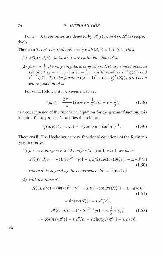
76 0 INTRODUCTION.

For x = 0, these series are denoted by H j,k(s), H j(s), Lv(s) respec-

tively.

Theorem 7. Let x be rational, x = dc

with (d, c) = 1, c > 1. Then

(1) H j,k(s, d/c), H j(s, d/c) are entire functions of s,

(2) for v , 12, the only singularities of Lv(s, d/c) are simple poles at

the point s1 = v + 12

and s2 =32− v with residues c−2vζ(2v) and

c2v−2ζ(2 − 2v); the function ((S − 1)2 − (v − 12)2)Lv(s, d/c) is an

entire function of s.

For what follows, it is convenient to set

γ(u, v) =22µ−1

πΓ(u + v − 1

2)Γ(u − v +

1

2); (1.48)

as a consequence of the functional equation for the gamma function, this

function for any u, v ∈ C satisfies the relation

γ(u, v)γ(1 − u, v) = −(cos2 πu − sin2 πv)−1. (1.49)

Theorem 8. The Hecke series have functional equations of the Riemann

type; moreover

1) for even integers k > 12 and for (d, c) = 1, c > 1, we have

H j,k(s, d/c) = −(4π/c)2s−1γ(1 − s, k/2) cos(πs)H j,k(1 − s,−d′/c)

(1.50)

where d′ is defined by the congruence dd′ ≡ 1(mod c)

2) with the same d′,

Lv(s, d/c) = (4π/c)2s−1γ(1 − s, v)− cos(πs)Lv(1 − s,−d/c)+

(1.51)

+ sin(πv)Lv(1 − s, d′/c),

H j(s, d/c) = (4π/c)2c−1γ(1 − s,1

2+ iχ j) (1.52)

− cos(πs)H j(1 − s, d′/c) + ǫ jch(πχ j)H j(1 − s, d/c).

68

1.9 The spectral mean of Hecke series. 77

We conclude with the simple but important consequence of the mul-

tiplicative relations (1.19) for Hecke operators : for Re s > 1+ |Re v− 12|,

we have

∞∑

n=1

τv(n)t j(n)

ns=

1

ζ(2s)H j(s + v − 1

2)H j(s − v +

1

2). (1.53)

If we replace t j(n) by τµ(n) (that corresponds to the continuous spec-

trum of the Hecke operators) then the well-known Ramanujan identity

will arise instead of (1.53):

∞∑

n=1

τv(n)τµ(n)

ns= (1.54)

=1

ζ(2s)ζ(s + v − µ)ζ(s + µ − v)ζ(s − v − µ + 1)ζ(s + v + µ − 1).

For this reason, equality (1.53) is a direct generalization of the Ra-

manujan identity; both will be essential for the estimate of the eighth

moment of the Riemann zeta-function.

1.9 The spectral mean of Hecke series.

Let N > 1 be an integer and let s, v be complex variables. We set

Z(d)

N(s, v; h) =

∑

j>1

α jt j(N)H j(s + v − 1

2)H j(s − v +

1

2)h(χ j) (1.55)

Z(d)

N(s, v; h) =

∑

j>1

ǫ jα jt j(N)H j(s + v − 1

2)H j(s − v +

1

2)h(χ j) (1.56)

(with α j = (ch(πχ j))−1|ρ j(1)|2). Here the summation is over the positive

discrete spectrum of the automorphic Laplacian and one assumes that

its eigenfunctions have been selected in such a manner that they are at

the same time eigenfunctions of the ring of Hecke operators and of the

reflection operator T−1(ǫ j = ±1 are the eigenvalues of T−1).Further, we define the square mean of the Hecke series over the

continuous spectrum by the equality

Z(c)

N(s, v; h) = (1.57)

78 0 INTRODUCTION.

=1

π

∞∫

−∞

ζ(s + v − 12+ ir)ζ(s + v − 1

2− ir)ζ(s − v + 1

2+ ir)ζ(s − v + 1

2− ir)

ζ(1 + 2ir)ζ(1 − 2ir)

× τ(1/2)+ir(N)h(r)dr

with the stipulation that, by means of integral (1.57), the function Z(c)N

69

is defined under the conditions

Re(s + v − 1

2) < 1,Re(s − v +

1

2) < 1.

If any one of the points s ± (v − 12) lies to the right hand side of the

unit line, then the integral (1.57) defines another function, connected

with Z(c)

Nby the Sokhotskii formulae. Fro example, if by Z

(c)

N, we denote

the function which is defined by (1.57) with Re s > 1, Re v = 12, then a

simple computation gives

Z(c)

N(s, v; h) = Z

(c)

N(s, v; h) + 4ζN(s, v)h(i(s − v − 1

2))+

+4ζN(s, 1 − v)h(i(s + v − 3

2))

where we have introduced the notation

ξN(s, v) =ζ(2s − 1)ζ(2v)

ζ(2 − 2s + 2v)τs−v(N)

and the regularity strip of h is assumed to be sufficiently wide for the

right hand side to make sense.

Now we need the mean with respect to the weights of the Hecke

series associated with regular cusp forms. For an integer k > 1, we set

ZN,k(s, v) = 2(−1)k Γ(2k − 1)

(4π)2k

v2k∑

j=1

|α j,2k(1)|2t j,2k(N) (1.58)

×H j,2k(s + v − 1

2)H j,2k(s − v +

1

2)

where t j,2k(N) is the eigenvalue of the N-th Hecke operator in the space

M2k of regular cusp forms of weight 2k, v2k = dim M2k; the empty sum

for 1 6 k 6 5 and k = 7 is assumed to be equal to zero.

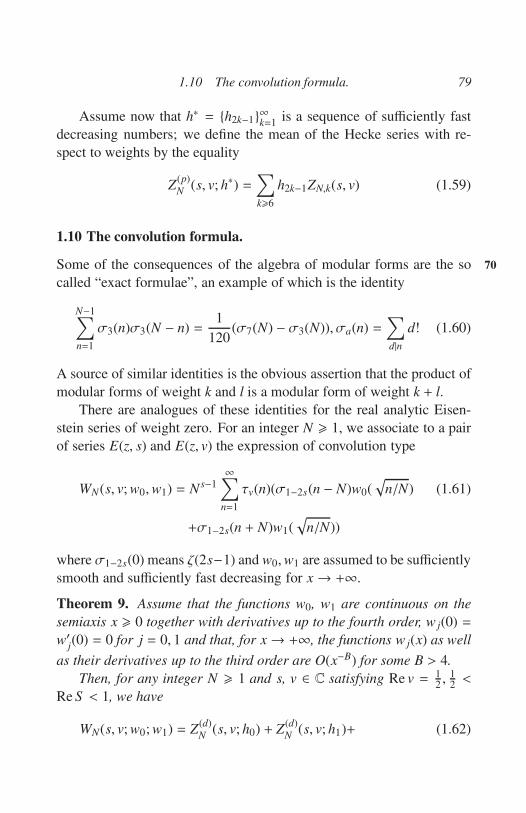
1.10 The convolution formula. 79

Assume now that h∗ = h2k−1∞k=1is a sequence of sufficiently fast

decreasing numbers; we define the mean of the Hecke series with re-

spect to weights by the equality

Z(p)

N(s, v; h∗) =

∑

k>6

h2k−1ZN,k(s, v) (1.59)

1.10 The convolution formula.

Some of the consequences of the algebra of modular forms are the so 70

called “exact formulae”, an example of which is the identity

N−1∑

n=1

σ3(n)σ3(N − n) =1

120(σ7(N) − σ3(N)), σa(n) =

∑

d|nd! (1.60)

A source of similar identities is the obvious assertion that the product of

modular forms of weight k and l is a modular form of weight k + l.

There are analogues of these identities for the real analytic Eisen-

stein series of weight zero. For an integer N > 1, we associate to a pair

of series E(z, s) and E(z, v) the expression of convolution type

WN(s, v; w0,w1) = N s−1∞∑

n=1

τv(n)(σ1−2s(n − N)w0(√

n/N) (1.61)

+σ1−2s(n + N)w1(√

n/N))

where σ1−2s(0) means ζ(2s−1) and w0,w1 are assumed to be sufficiently

smooth and sufficiently fast decreasing for x→ +∞.

Theorem 9. Assume that the functions w0, w1 are continuous on the

semiaxis x > 0 together with derivatives up to the fourth order, w j(0) =

w′j(0) = 0 for j = 0, 1 and that, for x→ +∞, the functions w j(x) as well

as their derivatives up to the third order are O(x−B) for some B > 4.

Then, for any integer N > 1 and s, v ∈ C satisfying Re v = 12, 1

2<

Re S < 1, we have

WN(s, v; w0; w1) = Z(d)

N(s, v; h0) + Z

(d)

N(s, v; h1)+ (1.62)

80 0 INTRODUCTION.

Z(c)

N(s, v; h0 + h1) + Z

(p)

N(s, v; h∗) + ζN(s, v)V(

1

2, v)+

ζN(s, 1 − v)V(1

2, 1 − v) + ζN(1 − s, v)V(s, v) + ζN(1 − s, 1 − v)|×

V(s, 1 − v)

where

ζN(s, v) =ζ(2s)ζ(2v)

ζ(2s + 2v)τs+v(N), (1.63)

V(s, v) = 2

∞∫

0

(|1 − x2|1−2s)w0(x)→ (1 + x2)1−2sw1(x))x2vdx (1.64)

and the column vector h(r; s, v) =

(

h0

h1

)

is defined in terms of w =

(

w0

w1

)

by the integral transform

h(r; s, v) = π

∞∫

0

(

k0(x, 12+ ir) 0

0 k1(x, 12+ ir)

)

(

x4π

)2s−1 × (1.65)

∞∫

0

(

k0(xy, v) k1(xy, v)

k1(xy, v) k0(xy, v)

)

w(y)ydydx

with the kernels71

k0(x, v) =J2v−1(x) − J1−2v(x)

2 cos(πv), (1.66)

k1(x, v) =2

πsin(πv)K2v−1(x).

Finally, the coefficients of the mean of the regular forms Z(ρ)

Nare

given by the relations

h2k−1 = 2(2k − 1)×

×∞

∫

0

J2k−1(x)

(

x

4π

)2s−1∞

∫

0

(k0(xy, v)w0(y) + k1(xy, v)w1(y))ydy dx.

1.11 Some consequences of the convolution formula. 81

1.11 Some consequences of the convolution formula.

The first example of the use of (1.62) is the additive divisor problem;

if we choose s = v = 1/2, w1 = 0 and w0 so that it is close to 1 in

the interval (0,√

T/N) (so that w0(√

n/N) will be close to 1 for n 6 T ),

then the left hand side of (1.62) gives the sum on the left side of (1.45).

Terms with the integral (1.64) are leading terms and all other terms give

the remainder term.

Of course, the asymptotic formula for the additive divisor problem is

crucial for the investigation of the fourth power moment of the Riemann

zeta-function. A consequence of (1.62) in this direction is the following

Theorem. (N. Zavorotnyi, 1987). Let T → +∞; then, for any ǫ > 0, we

haveT

∫

0

|ζ(1

2+ it)|4dt = T P4(log T ) + O(T 2/3+ǫ ) (1.67)

where P4(z) is a polynomial in z of the fourth degree with constant coef-

ficients.

We can consider the functions h0 and h1 in (1.62) as given; the fol- 72

lowing unusual integral transform is useful to invert (1.62).

Let us define the matrix kernel K(x, v) by the equality

K(x, v) =

(

k0(x, v) k1(x, v)

k1(x, v) k0(x, v)

)

(1.68)

with k0, k1 from (1.66). Now we shall consider the matrix equation

w(x) =

∞∫

0

K(xy, v)u(y)√

xydy (1.69)

where w =

(

w0

w1

)

(x), u =

(

u0

u1

)

(x).

82 0 INTRODUCTION.

Theorem 10. Let Re v = 12

and w ∈ L2(0,∞) in the sense that w0,w′1∈

L2(0,∞). Then there exists a unique solution u in L2(0,∞) of the equa-

tion (1.69) and this solution is given by the formula

u(x) =

∞∫

0

K(xy, u)w(y)√

xydy (1.70)

where the integral is understood in the mean-square sense.

Now, as a special case of the convolution formula (1.62), we have

the following asymptotic formulae.

Theorem 11. Let T → +∞. Then for a fixed σ and t ∈ R with 12< σ <

1, we have

∑

χ j6T

α j|H j(σ + it)|2 = T 2

π2(ζ(2σ) +

ζ(2 − 2σ)

2(1 − σ)

(

T 2

2π

)1−2σ

) + O(T log T )

(1.71)

while, for σ = 12

the right-hand side has to be replaced by

2T 2

π2(log T + 2γ − 1 + 2log(2π)) + O(T log T ). (1.72)

1.12 The explicit formulae for the transformation (1.65)

We rewrite equality (1.65) in the form

h =

∞∫

0

A(r, y; s, v)

(

w0

w1

)

(y)dy, A =

(

A00 A01

A10 A11

)

, (1.73)

where the matrix kernel A, under the conditions Re v = 12, 1

2< Re s < 1,

|Iimr| < Re s, is determined by the integrals that appear in the term-by-73

term integration in (1.65). All these integrals are given in tables (these

are the Weber-Schafheitlin integrals); we will be needing the following

explicit form for the kernels A j,l, j, l = 0, 1.

1.12 The explicit formulae for the transformation (1.65) 83

Proposition 1. Let us denote, for Re v = 12, 1

2< Re s < 1, | Im r| < Re s

a = s + v − 1

2+ ir, b = s − v +

1

2+ ir, c = 1 + 2ir, (1.74)

a′ = s + v = −1

2− ir, b′ = s − v +

1

2− ir, c′ = 1 − 2ir. (1.75)

Then, for 0 < y < 1, we have

(2π)2s−1A00(r, y; s, v) := πy

∞∫

0

k0(x,1

2+ ir)k0(xy, v)(

x

2)2s−1dx (1.76)

=1

2 cos(πv)

Γ(a)Γ(a′)

Γ(2v)y2vF(a, a′; 2v; y2) sin π(s + v)+

+Γ(b)Γ(b′)

Γ(2 − 2v)y2−2vF(b, b′; 2 − 2v; y2) sin π(s − v)

and for y > 1,

(2π)2s−1A00(r, y; s, v) = (1.77)

=iy1−2s

2sh(πr)

Γ(a)Γ(b)

yc−1Γ(c)F

(

a, b; c;1

y2

)

cos π(s + ir)−

−Γ(a′)Γ(b′)

yc′−1Γ(c′)F

(

a′, b′; c′;1

y2

)

cos π(s − ir)

At the same time, for all y > 0, we have

(2π)2s−1A00(r, y; s, v) = sin(πs)Γ(2s − 1)y2v |1 − y2|1−2s× (1.78)

F(1 − b, 1 − b′; 2 − 2s; 1 − y2) +Γ(a)Γ(a′)Γ(b)Γ(b′)

2πΓ(2s) cos(πs)×

(ch2πr + sin2 πv − sin2 πs)y2vF(a, a′; 2s; 1 − y2)

where, in the first term, the absolute value sign combines the two cases

y < 1 and y > 1.

Proposition 2. With the same parameters, we have 74

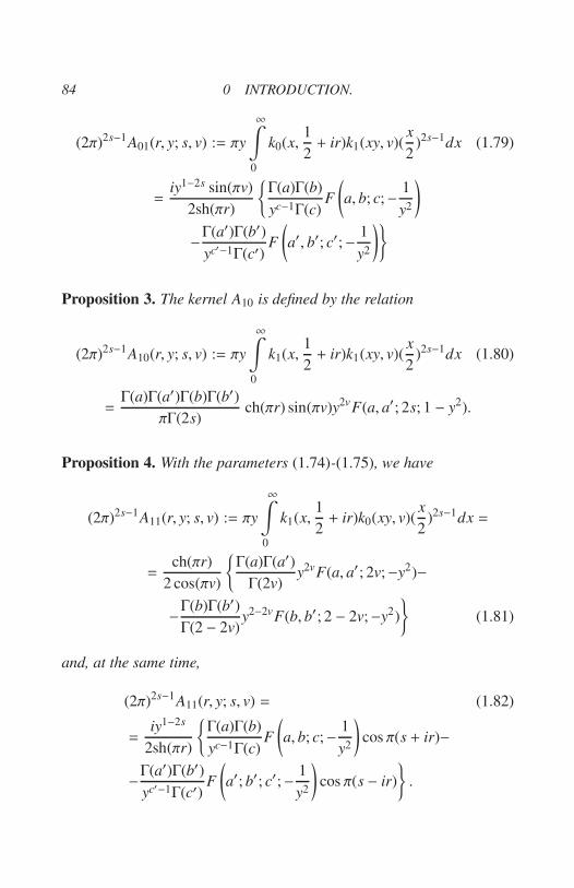
84 0 INTRODUCTION.

(2π)2s−1A01(r, y; s, v) := πy

∞∫

0

k0(x,1

2+ ir)k1(xy, v)(

x

2)2s−1dx (1.79)

=iy1−2s sin(πv)

2sh(πr)

Γ(a)Γ(b)

yc−1Γ(c)F

(

a, b; c;− 1

y2

)

−Γ(a′)Γ(b′)

yc′−1Γ(c′)F

(

a′, b′; c′;− 1

y2

)

Proposition 3. The kernel A10 is defined by the relation

(2π)2s−1A10(r, y; s, v) := πy

∞∫

0

k1(x,1

2+ ir)k1(xy, v)(

x

2)2s−1dx (1.80)

=Γ(a)Γ(a′)Γ(b)Γ(b′)

πΓ(2s)ch(πr) sin(πv)y2vF(a, a′; 2s; 1 − y2).

Proposition 4. With the parameters (1.74)-(1.75), we have

(2π)2s−1A11(r, y; s, v) := πy

∞∫

0

k1(x,1

2+ ir)k0(xy, v)(

x

2)2s−1dx =

=ch(πr)

2 cos(πv)

Γ(a)Γ(a′)

Γ(2v)y2vF(a, a′; 2v;−y2)−

−Γ(b)Γ(b′)

Γ(2 − 2v)y2−2vF(b, b′; 2 − 2v;−y2)

(1.81)

and, at the same time,

(2π)2s−1A11(r, y; s, v) = (1.82)

=iy1−2s

2sh(πr)

Γ(a)Γ(b)

yc−1Γ(c)F

(

a, b; c;− 1

y2

)

cos π(s + ir)−

−Γ(a′)Γ(b′)

yc′−1Γ(c′)F

(

a′; b′; c′;− 1

y2

)

cos π(s − ir)

.

1.12 The explicit formulae for the transformation (1.65) 85

Proposition 5. Let us write the quantities h2k−1 in (1.62) as

h2k−1(s, v) =

∞∫

0

(A0k(y; s, v)w0(y) + A1

k(y; s, v)w1(y))dy. (1.83)

Then, for 0 < y < 1, 75

(2π)2s−1A0k(y; s, v) = (1.84)

2k − 1

cos(πv)

Γ(s + v − 1 + k)

Γ(2v)Γ(1 − s − v + k)y2vF(k + s + v − 1, s + v − k; 2v; y2)−

− Γ(k + s − v)

Γ(2 − 2v)Γ(v − s + k)y2−2vF(k + s − v, s + 1 − v − k; 2 − 2v; y2)

and, for y > 1,

(2π)2s−1A0k(y; s, n) = (1.85)

(−1)k−1 sin(πs)

πy2k+2s−2

Γ(k + s + v − 1)Γ(k + s − v)

Γ(2k − 1)×

F

(

k + s + v − 1, k + s − v; 2k;1

y2

)

.

For the second kernel in (1.83), we have

(2π)2s−1A1k(y; s, v) = (1.86)

= − sin(πv)

πy2k+2s−2

Γ(k + s + v − 1)Γ(k + s − v)

Γ(2k − 1)×

F

(

k + s + v − 1, k + s − v; 2k;− 1

y2

)

Part II. The eighth moment of the Riemannzeta-function.

86 0 INTRODUCTION.

2.1 The result and a rough sketch of the proof.

Since the question about the true order of zeta-function on the critical

line is open even today - and it will be so in the foreseeable future-, a

sizeable part of the theory of the Riemann zeta-function is an attempt to

present the asymptotic mean value

1

T

T∫

0

|ζ(1

2+ it)|2kdt, k = 1, 2, . . . (2.1)

The case k = 4 will be investigated here; for this case, the following

new estimate will be given.

Theorem 12. There is an absolute constant B such that76

T∫

0

|ζ(1

2+ it)|8dt ≪ T (log T )B (2.2)

when T → +∞.

Furthermore, the same estimate is valid for the fourth power mo-

ment of the Hecke series of the discrete spectrum of the automorphic

Laplacian. Namely, we have

Theorem 13. For every fixed j > 1 with the same B as in (2.2), we have

α j

T∫

0

|H j(1

2+ it)|4dt ≪ T (log T )B−6, T → +∞. (2.3)

To give these estimates we shall consider the fourth spectral moment

of the Hecke series over the discrete and continuous spectrum. The one

over the discrete spectrum is defined by

Zdis

(

s, v

ρ, µ

∣

∣

∣

∣

∣

∣

h

)

= (2.4)

∑

j>1

α j

H j(s + v − 12)H j(s − v + 1

2)H j(ρ + µ − 1

2)H j(ρ − µ + 1

2)

ζ(2s)ζ(2ρ)h(χ j)

2.1 The result and a rough sketch of the proof. 87

with

α j = (ch(πχ j))−1|ρ j(1)|2. (2.5)

Of course, this function results from the following summation (see

the generalized Ramanujan identity (1.53)):

Zdis

(

s, v

ρ, µ

∣

∣

∣

∣

∣

∣

h

)

=

∑

n,m>1

τv(n)

ns

τµ(m)

mρ

∑

j>1

α jt j(n)t j(m)h(χ j)

(2.6)

when Re s > Re v − 12| + 1, Re ρ > |Re µ − 1

2| + 1. The function

ζ(2s)ζ(2ρ)Zdis

(

s, v

ρ, µ

∣

∣

∣

∣

∣

∣

h

)

is regular in some domain of the kind Re s > s0’ Re ρ > ρ0, where s′0ρ0

depend on the order of decay of the function |h(r)| for |r| → +∞.

We shall denote by Zdis

(

s, v

ρ, µ

∣

∣

∣

∣

∣

∣

h

)

the expression obtained on replac-

ing α j by ǫ jα j in (2.6):

Zdis

(

s, v

ρ, µ

∣

∣

∣

∣

∣

∣

h

)

=

∑

n,m>1

τv(n)

n2

τµ(m)

mρ

∑

j>1

ǫ jα jt j(n)t j(m)h(χ j)

(2.7)

In the same manner as in (2.6), we define the fourth spectral moment 77

over the continuous spectrum by

Zcon0

(

s, v

ρ, µ

∣

∣

∣

∣

∣

∣

h

)

=1

4π

∞∫

−∞

Z(s; v,1

2+ ir)Z(ρ; µ,

1

2+ ir)

h(r)dr

ζ(1 + 2ir)ζ(1 − 2ir)

(2.8)

where we assume Re(s ± (v − 12)) > 1, Re(ρ ± (µ − 1

2)) > 1 and the

notation z is introduced for the right side of the well-known Ramanujan

identity:

z(s; v, µ) =

∞∑

n=1

τv(n)τµ(n)

ns(2.9)

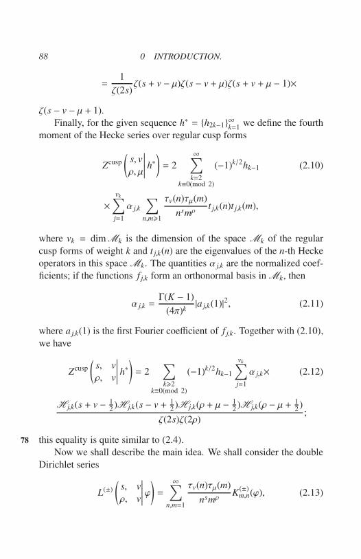
88 0 INTRODUCTION.

=1

ζ(2s)ζ(s + v − µ)ζ(s − v + µ)ζ(s + v + µ − 1)×

ζ(s − v − µ + 1).

Finally, for the given sequence h∗ = h2k−1∞k=1we define the fourth

moment of the Hecke series over regular cusp forms

Zcusp

(

s, v

ρ, µ

∣

∣

∣

∣

∣

∣

h∗)

= 2

∞∑

k=2k≡0(mod 2)

(−1)k/2hk−1 (2.10)

×vk∑

j=1

α j,k

∑

n,m>1

τv(n)τµ(m)

nsmρt j,k(n)t j,k(m),

where vk = dim Mk is the dimension of the space Mk of the regular

cusp forms of weight k and t j,k(n) are the eigenvalues of the n-th Hecke

operators in this space Mk. The quantities α j,k are the normalized coef-

ficients; if the functions f j,k form an orthonormal basis in Mk, then

α j,k =Γ(K − 1)

(4π)k|a j,k(1)|2, (2.11)

where a j,k(1) is the first Fourier coefficient of f j,k. Together with (2.10),

we have

Zcusp

(

s, v

ρ, v

∣

∣

∣

∣

∣

∣

h∗)

= 2∑

k>2k≡0(mod 2)

(−1)k/2hk−1

vk∑

j=1

α j,k× (2.12)

H j,k(s + v − 12)H j,k(s − v + 1

2)H j,k(ρ + µ − 1

2)H j,k(ρ − µ + 1

2)

ζ(2s)ζ(2ρ);

this equality is quite similar to (2.4).78

Now we shall describe the main idea. We shall consider the double

Dirichlet series

L(±)

(

s, v

ρ, v

∣

∣

∣

∣

∣

∣

ϕ

)

=

∞∑

n,m=1

τv(n)τµ(m)

nsmρK

(±)m,n(ϕ), (2.13)

2.1 The result and a rough sketch of the proof. 89

where the coefficients are sums of Kloosterman sums with the smooth

“test” function ϕ:

K(±)m,n(ϕ) =

∑

c>1

1

cS (n,±m; c)ϕ

(

4π√

nm

c

)

. (2.14)

Since there is a functional equation of the Riemann type for the

Dirichlet series

Lv

(

S ,a

c

)

=

∞∑

n=1

n−sτv(n)e(na

c), e(x) := e2πix,

when a, c ∈ Z are coprime and this equation connects Lv(S , ac) with

Lv(1− s,± a′c′ ), aa′ ≡ 1(mod c), a functional equation has to exist for the

functions L(±)

(

s, v

ρ, µ

∣

∣

∣

∣

∣

∣

ϕ

)

; it will connect this function with the functions

of the same kind L(±)

(

ρ, v

s, µ

∣

∣

∣

∣

∣

∣

ϕ

)

for an appropriate ϕ. As a consequence

of the sum formula for Kloosterman sums, it means that there is a func-

tional equation for the function

Z

(

s, v

ρ, µ

∣

∣

∣

∣

∣

∣

h

)

= Zdis

(

s, v

ρ, µ

∣

∣

∣

∣

∣

∣

h

)

+ Zcon

(

s, v

ρ, µ

∣

∣

∣

∣

∣

∣

h

)

; (2.15)

roughly speaking, this equation (which will be written below in detail)

is the result of the exchange of s and ρ and the replacement of h by some

integral transform.

Now, on the left side of this functional equation, for the special case

s = µ =1

2, ρ = v =

1

2+ it, t ∈ R is large and positive, (2.16)

we have in the continuous spectrum the product

ζ3(1

2+ it + ir)ζ3(

1

2+ it − ir)ζ(

1

2− it + ir)ζ(

1

2− it − ir) (2.17)

and the other product will be on the right side; namely, we have therein

ζ3(1

2+ ir)ζ3(

1

2− ir)ζ(

1

2+ 2it + 2ir)ζ(

1

2+ 2it − 2ir). (2.18)

90 0 INTRODUCTION.

After this specialization, we shall choose the special function h essen-

tially as exp(−αr2) with a fixed positive α. Then the essential part of the

interval of the integration is |r| ≪ (log t)(1/2). The length of this interval

is small in comparison to the large t and for this reason, (using the Rie-

mann functional equation), we can reduce the main term of our product

on the left side to the form

|ζ4(1

2+ it + ir)ζ4(

1

2+ it − ir)|.

It means that we may hope to estimate the integral79

ǫ∫

−ǫ

∞∫

0

ωT (t)|ζ4(1

2+ it + ir)ζ4(

1

2+ it − ir)|dtr2dr (2.19)

for arbitrary small positive ǫ, if ωT (t) is the smooth function which is

not zero for t ∈ (T, 2T ) only and close to 1 when 54T 6 t 6 7

4T (see

picture).

figure 79 page

The main term will be close to the integral

ǫ3

∞∫

0

ωT (t)|ζ(1

2+ it)|∞dt

if ǫ ≪ (log T )−2 (see subsection (2.4)); so we have the eighth moment

of the Riemann zeta-function here. At the same time, the contribution

of the discrete spectrum is positive too. Hence the desired conclusion

follows if the integrals on the right side can be estimated with sufficient

accuracy.

But the integrand for these integrals contains one Hecke series only;

so the integration may be done asymptotically. As a result, we shall

reduce the problem of the estimate of the eighth power moment to the

problem of the estimate for the fourth spectral moment. It is sufficient

to prove our theorem for the latter.

2.2 The first functional equation 91

In the conclusion of the introduction of the second part, we shall

note that the estimate

|ζ(1

2+ it)| ≪ |t|1/8(log |t|)B1 , , t → ±∞,

follows from (2.2), B1 =18

B + 12.

It is preceptibly better than the last achievement in the long chain of

the results of the kind |ζ(12+ it)≪ |t|γ.

2.2 The first functional equation80

Since the sum Zdis+ Zcon is connected with the sum of Kloosterman

sums, we shall consider the triple sum

L(±)

(

s, v

ρ, µ

∣

∣

∣

∣

∣

∣

ϕ

)

=

∞∑

n,m=1

τv(n)τµ(m)

nsmρK

(±)n,m(ϕ). (3.1)

Here the notation (2.14) is used and we assume that a function ϕ is

“good” namely, the Mellin transform ϕ(u)

ϕ(u) =

∞∫

0

ϕ(x)xu−1dx, (3.2)

is regular in the strip −α0 6 Re u 6 α1 with positive α0, α1 and |ϕ(u)|decreases sufficiently rapidly in this strip. For this reason, we can write

ϕ(x) =1

iπ

∞∫

iπ

∞∫

(α)

ϕ(2u)x−2udu, x > 0, (3.3)

where∞∫

(α)

stands for the integral over the line Re u = α. As we have

|S (n,m; c)| ≪ c1/2(n,m, c)d(c),

92 0 INTRODUCTION.

the triple sum (3.1) converges absolutely if α < − 14

and both Re(s + α),

Re(ρ+α) are larger than 1. For this case, we have, for the sum (3.1), the

following expression

L(±)

(

s, v

ρ, µ

∣

∣

∣

∣

∣

∣

ϕ

)

=1

iπ

∑

c>1

1

c× (3.4)

∑

ad≡1(mod c)

∫

(α)

Lv(s + u,a

c)Lµ(ρ + µ,±d

c)(c/4π)2uϕ(2µ)du.

Now we shall integrate over the line Re u = α0 where α0 will be chosenso that both Re(s+α0), Re(ρ+α0) are negative. Taking into account thecontribution from the poles, we have

L(±)

(

s, v

ρ, µ

∣

∣

∣

∣

∣

∣

ϕ

)

(3.5)

= 2∑

c>1

∑

ad≡1(mod c)

(4π)2s−1

c2s

(

ζ(2v)

(4π)2vLµ(ρ − s + v +

1

2,±d/c)ϕ(2v + 1 − 2s)+

+ζ(2 − 2v)

(4π)2−2vLµ(ρ − s +

3

2− v,±d/c)ϕ(3 − 2v − 2s)

)

+

+(4π)2ρ−1

c2ρ

((

ζ(2µ)

(4π)2µLv(s − ρ + µ + 1

2, a/c)

)

×

ϕ(2µ + 1 − 2ρ) +ζ(2 − 2µ)

(4π)2−2µLv(s − ρ + 3

2− µ, a/c)ϕ(3 − 2µ − 2ρ)

)

+

+1

iπ

∑

c>1

1

c

∑

ad≡1(mod c)

∫

α0

Lv(s + u, a/c)Lµ(ρ + u,±d/c)(c

4π)2uϕ(2u)du.

In the last term, we shall use the functional equation (1.51). If the sign81

“plus” is taken, then it gives for our sum the expression

∑

c>1

1

c

∑

n,m>1

τv(n)τµ(m)

nρms(S (n,m; c)Φ0

(

4π√

nm

c

)

+ (3.6)

+S (n,−m; c)Φ1

(

4π√

nm

c

))

2.2 The first functional equation 93

where

Φ0 = Φ0(x; s, v; ρ, µ) = (3.7)

=1

iπx2s+2ρ−2

∫

(α0)

γ(1 − s − u, v)γ(1 − ρ − u, µ)×

(cos π(s + µ) cos π(ρ + u) + sin(πv) sin(πµ))x2uϕ(2u)du,

Φ1 = Φ1(x; s, v; ρ, µ) = (3.8)

= − 1

iπx2s+2ρ−2

∫

(α0)

γ(1 − s − u, v)γ(1 − ρ − u, µ)(sin(πµ)×

cos π(s + u) + sin(πv) cos π(ρ + µ)x2uϕ(2u)du,

Of course, when the sign “minus” is taken in (3.5), then the same

function s Φ0 and Φ1 are the coefficients, but Φ0 will occur with

S (n,−m; c) and Φ1 with S (n,m; c).

We have Φ j(x) = O(x2 min(Re s,Re ρ)) as x → 0+ and these functions

are bounded when x is large. For this reason, the triple sums in (3.6)

converge absolutely and we can again interchange the order of the sum-

mations. Hence we have, in (3.7), the sum

L(+)

(

ρ, v

s, µ

∣

∣

∣

∣

∣

∣

Φ0

)

+ L(−)

(

ρ, v

s, µ

∣

∣

∣

∣

∣

∣

Φ1

)

(3.9)

for the case “+” on the left side (3.5) and

L(+)

(

ρ, v

s, µ

∣

∣

∣

∣

∣

∣

Φ1

)

+ L(−)

(

ρ, v

s, µ

∣

∣

∣

∣

∣

∣

Φ0

)

(3.10)

for the other case. 82

Now we are ready to give the first functional equation.

Theorem 14. Let Re v = Re µ = 12

and let, for some positive δ < 14, the

variables s, ρ satisfy 54< Re s, Re ρ < 5

4+δ. Let ϕ : [0,∞)→ C have the

Mellin transform ϕ(u) such that ϕ(u) is regular for − 32− 2δ 6 Re u 6 2.

Then we have

L(+)

(

s, v

ρ, µ

∣

∣

∣

∣

∣

∣

ϕ

)

= L(+)

(

ρ, v

s, µ

∣

∣

∣

∣

∣

∣

ϕ0

)

L(−)

(

ρ, v

s, µ

∣

∣

∣

∣

∣

∣

ϕ1

)

+ (3.11)

94 0 INTRODUCTION.

+2(4π)2s−1

ζ(2s)

(

ζ(2v)

(4π)2vz(ρ + v; s, µ)ϕ(2v + 1 − 2s)+

+ζ(2 − 2v)

(4π)2−2vz(ρ + 1 − v; s, µ)ϕ(3 − 2v − 2s)

)

+

+2(4π)2ρ−1

ζ(2ρ)

(

ζ(2(µ)

(4π)2µz(s + µ; ρ, v)ϕ(2µ + 1 − 2ρ)+

+ζ(2 − 2µ)

(4π)2−2µz(s + 1 − µ; ρ, v)ϕ(3 − 2µ − 2rho)

)

,

where Φ0, Φ1 are defined by the following integral transformations

Φ0(x) ≡ Φ0(x; s, v; ρ, µ) = x2s+2ρ−2

∞"

0

(k0(ξ, v)k0(η, µ)+ (3.12)

k1(ξ, v)k1(η, µ))ϕ(ξη/x)ξ1−2sη1−2ρdξdη

Φ1(x) ≡ Φ1(x; s, v; ρ, µ) = x2s+2ρ−2

∞"

0

(k0(ξ, v)k0(η, µ)+ (3.13)

k1(ξ, v)k0(η, µ))ϕ(ξη/x)ξ1−2sη1−2ρdξdη.

Of course, it is the same as what we have in (3.5). If Re ρ > Re s,

then in the first term on the right side of (3.5), one has the sum

∑

c>1

1

c2s

∞∑

n=1

τµ(n)

nρ−s+v+(1/2)S (0, n; c) = (3.14)

=1

ζ(2s)

∞∑

n=1

τµ(n)σ1−2s(n)

nρ−s+v+(1/2)=

z(ρ + v; s, µ)

ζ(2s)

On the right side, we have a meromorphic function of ρ in the half-83

plane Re ρ > 12; so this equality holds for the analytic continuation of

the initial sum

∑

c>1

1

c2s

∑

(d,c)=1

Lµ

(

ρ − s + v +1

2,

d

c

)

(3.15)

2.3 The main functional equation: the preparations. 95

if we can be sure that this function is meromorphic not only for Re ρ >

Re s. It is sufficient for this to know that Lµ(w, dc) as a function of c is

bounded in the mean when Re w > 12

(except at the poles). But this fact

is a consequence of the Bombieri-Vinogradov inequality which asserts

that

∑

16c6M

∑

(d,c)=1

∣

∣

∣

∣

∣

∣

∣

P+Q∑

)n=Pb(n)e(nd

c)

∣

∣

∣

∣

∣

∣

∣

2

≪ max(Q, M2)

P+Q∑

n=P

|b(n)|2 (3.16)

for an arbitrary sequence of complex numbers b(n).

Now one can check that relations (3.12) - (3.13) and (3.7) - (3.8) are

idential. We have the tabular integrals

∞∫

0

k0(x, v)xw−1dx = γ

(

w

2, v

)

cos

(

πw

2

)

, 0 < Re w <3

2, (3.17)

∞∫

0

k1(x, v)xw−1dx = γ

(

w

2, v

)

sin(πv),Re w > 0, (3.18)

After writing ϕ in (3.12)-(3.13) as the Mellin integral,

ϕ

(

ξη

x

)

=1

iπ

∫

ϕ(2u)

(

x

ξη

)2u

du,

we shall come to an absolutely convergent triple integral if

max

(

3

4− Re s,

3

4− Re ρ

)

< Re u < min(1 − Re s, 1 − Re ρ).

Hence there is a non-empty strip where we can integrate in any order;

this gives our relations for Φ0 and Φ1.

2.3 The main functional equation: the preparations.

For the given function h(r) and the sequence h∗ := h2k−1∞k−1, we shall

consider the function

Z

(

s, v

ρ, µ

∣

∣

∣

∣

∣

∣

h

)

= Zdis

(

s, v

ρ, µ

∣

∣

∣

∣

∣

∣

h

)

+ Zcon0

(

s, v

ρ, µ

∣

∣

∣

∣

∣

∣

h

)

+ Zcusp

(

s, v

ρ, µ

∣

∣

∣

∣

∣

∣

h∗)

.

(4.1)

96 0 INTRODUCTION.

When Re s, Re ρ > 1, this function is equal to84

∞∑

n,m=1

τv(n)τµ(m)

nsmρK(+)

n,m(ϕ) +δn,m

π2

∞∫

−∞

rth(πr)h(r)dr = (4.2)

= L(+)

(

s, v

ρ, µ

∣

∣

∣

∣

∣

∣

ϕ

)

+1

π2z(s + ρ; v, µ)

∞∫

−∞

rth(πr)h(r)dr

where ϕ corresponds to h and h∗ in the sense of Theorems 1 and 4.

Our intention must be clear now; we shall use the first functional

equation for L(+) and after this, the analytic continuation of both sides

will be carried out.

Firstly, it is convenient to write the analytic continuation for the

function Zcon0

. Let us denote by Zcon the integral in which (under the

usual conditions Re v = Re µ = 12) we have Re s < 1, Re ρ < 1. Then

Zcon0

and Zcon are connected by the following relation.

Proposition 6. Let h be a regular function on the sufficiently wide strip

| Im r| 6 ∆, ∆ > 12. Then for Re s > 1, Re ρ < 1, the meromorphic

continuation of Zcon0

(

s, v

ρ, µ

∣

∣

∣

∣

∣

∣

h

)

is given by the equality.

Zcon0

(

s, v

ρ, µ

∣

∣

∣

∣

∣

∣

h

)

− Zcon

(

s, v

ρ, µ

∣

∣

∣

∣

∣

∣

h

)

+ (4.3)

+ζ(2s − 1)

ζ(2s)

ζ(2v)z(ρ; µ, 1 − s + v)

ζ(2 + 2v − 2s)h(i(s − v − 1

2))

+

+ζ(2 − 2v)z(ρ; µ, 2 − s − v)

ζ(4 − 2v − 2s)h(i(s + v − 3

2))+

+ζ(2ρ − 1)

ζ(2ρ)

ζ(2µ)z(s; v, 1 − ρ + µ)

ζ(z + 2µ − 2ρ)h(i(ρ − µ − 1

2))+

+ζ(2 − 2µ)z(s; v, 2 − ρ − µ)

ζ(4 − 2µ − 2ρ)h(i(ρ + µ − 3

2))

.

Really Zcon0

is a Cauchy integral, because ζ has only a simple pole.

2.3 The main functional equation: the preparations. 97

so the poles of z(s; v, 12+ ir) are the points r j, 1 6 j 6 4, with

ir1 =1

2− s + v, ir2 =

3

2− s − v, r3 = −r1, r4 = −r2.

When Re s > 1 the points r1, r2 are lying above the real axis and if

Re s < 1, they are below the same. Now one can deform the path of

integration (see picture; the deformation must be so small that the func-

tions ζ(1 + ±2ir) have no zeros inside the lines; it is possible, since the 85

Riemann zeta-function has no zeros on the line Re s = 1) and the desired

conclusion is the result of the direct calculation of the residues.

figure 85 page

The next step is the representation of the functions L(±)

(

ρ, v

s, µ

∣

∣

∣

∣

∣

∣

Φ j

)

as a bilinear form in the eigenvalues of the Hecke operators. For this,

we need to consider the integral transforms of Theorems (4) and (1).

The situation now is the following : for a given h, we define ϕ by the

transformation (1.27), or what is the same, by the equality

ϕ(x) =1

π

∞∫

−∞

k0(x,1

2+ iu)uth(πu)h(u)du, (4.4)

and thereafter, we should calculate the integrals Φ0 and Φ1 in (3.12) and

(3.13) with this ϕ and finally the integral transformations

h0(r) ≡ h0(r; s, v; ρ, µ) = π

∞∫

0

k0(x,1

2+ ir)Φ0(x)

dx

x, (4.5)

h1(r) ≡ h1(r; s, v; ρ, µ) = π

∞∫

0

k1(x,1

2+ ir)Φ1(x)

dx

x. (4.6)

In order to obtain an asymptotic estimate, it is preferable to diminish

the length of the sequence of these integral transformations; we give the

results in the following

98 0 INTRODUCTION.

Proposition 7. Assume that the function h(u) is even and regular in the

strip | Im u| 6 32

and h has zeros at u = ± i2. Let |h| decrease as O(|u|−B)

for some B > 4 when |u| → ∞ with | Im u| 6 32. Then the function h0 is

given by the integral transform

h0(r) =2

π2

∞∫

−∞

B0(r; u; ρ, v, µ; s)u th(πu)h(u)du (4.7)

where, with the notation from (1.78), (1.79), we have, for Re v = Re µ =12, 1

26 Re s, Re ρ < 1

B0(r, u; ρ, v, µ; s) =

∞∫

0

(A00(r, ξ, ρ, v)A00(u,1

ξ; 1 − ρ, µ)+ (4.8)

A01(r, ξ; ρ, v)A01(u,1

ξ; 1 − ρ, µ))ξ2ρ−2s−1dξ

and here86

B0(r, u; ρ, v, µ; s) = B0(r, u; s, µ, v; ρ). (4.9)

Proposition 8. Under the same conditions

h1(r) =2

π2

∞∫

−∞

B1(r, u; s, µ, v; ρ)u th(πu)h(u)du (4.10)

where, with the notation (1.78), (1.80),

B1(r, u; s, µ, v; ρ) = B1(r, u; ρ, v, µ; s) = (4.11)

=

∞∫

0

(A10(r, ξ, s, µ)A00(u,1

ξ; 1 − s, v)+

+ A11(r, ξ, s, µ)A01(u,1

ξ; 1 − s, v))ξ2s−2ρ−1dξ.

Both the propositions result from term-by-term integration in the

corresponding multiple integrals; it is sufficient to consider the first re-

lation (4.7).

2.3 The main functional equation: the preparations. 99

First of all, the function ϕ in (4.4), for our case, is O(x3) when x→ 0

and O(x−(1/2)) for x → +∞. Furthermore, the Mellin transform of this

function, which is defined by the integral

ϕ(w) : =

∞∫

0

ϕ(x)xw−1dx = (4.12)

=2

πcos

(

πw

2

)

∞∫

−∞

γ

(

w

2,

1

2+ iu

)

u th(πu)h(u)du

is regular for Re w > −3 and |ϕ(w)| may be estimated as O(|w|Re w−1)

when |w| → ∞ and Re w is fixed.For this reason, the integrals (3.7) - (3.8) are absolutely convergent

if α0 < Re(s+ ρ)− 1. At the same time, both the integrals with k j(x, 12+

ir)× x2s+2ρ+2u−3 for j = 0, 1 are absolutely convergent for 1−Re(s+ρ) <

Re u < 54− Re(s + ρ). If Re(s + ρ) > 1

2, we can choose α0 in such a

manner that the term-by-term integration would be valid in the integralswhich will arise on replacing Φ j in (4.5) and (4.6) by the representations(3.7) and (3.8). In this way, we have

h0(r) =2i

π2

∞∫

−∞

uth (πu)h(u)× (4.13)

×∫

(α0)

γ(s + ρ + w − 1,1

2+ ir)γ(1 − s − w, v)γ(1 − ρ − w, µ)γ(w,

1

2+ iu)×

× cos(πw) sin π(s + ρ + w)(cosπ(s + w) sin(πv)+

+ cos π(ρ + w) sin(πµ))dwdu.

After this, it is sufficient to check that two representations are identical 87

for Re s, Re ρ < 1; but this results immediately from the explicit formu-

lae for the Mellin transforms of the kernels k j and the definitions of the

kernels Ak,l.

To finish the preparations, it remains to write the coefficients in the

sum over the regular cusps for the sum of Kloosterman sums with weight

function Φ0 and, finally, to consider the analytic continuation of the

function Zcon0

(

ρ, v

s, µ

∣

∣

∣

∣

∣

∣

h0 + h1

)

.

100 0 INTRODUCTION.

The first is not difficult; it is sufficient to do the formal substitution

r = i(k − 12) in the expression for h0(r) and to note the well-known

limiting case

limc→−2k

(Γ(c))−1F(a, b; c; z) =Γ(a + 2k + 1)Γ(b + 2k + 1)

Γ(2k + 2)× (4.14)

×z2k+1F(a + 2k + 1, b + 2k + 1; 2k + 2; z)

which holds for a positive integer k.

The analytic continuation is given by the same kind of relation as in

(4.3); so it is sufficient to calculate the values (h0 +h1)(i(s−1)± (µ− 12))

and (h0 + h1)(i(ρ − 1) ± (v − 12)).

Proposition 9. Let h be the same function as in Proposition (7); then,

for 12< Re s, Re ρ < 1, Re v = Re µ = 1

2, we have

(h0 + h1)(i(ρ − v − 1

2)) =

2

π2

∞∫

−∞

u th (πu)h(u)B0(u; ρ, µ, s − v)du (4.15)

where

B0(u; ρ, µ,w) = (2π)1−2ρ sin(πρ)Γ(2ρ − 1)× (4.16)

×∞

∫

0

(|1 − ξ2|1−2ρA00(u, 1/ξ; 1 − ρ, µ)+

+ (1 + ξ2)1−2ρA01(u.1/ξ; 1 − ρ, µ))ξ2ρ−2w−1dξ.

88

This relation is a consequence of the explicit formulae for the ker-

nels Ak,l. If r = i(ρ − v − 12), then, in these formulae, we have

a = 2v, b = 1, c = 2 − 2ρ + 2v; a′ = 2ρ − 1, b′ = 2ρ − 2v, c′ = 2ρ − 2v.

Now, we have, for the special case of the hypergeometric functions,

F(0, b; c; z) ≡ 1 and F(a, b; b; z) = (1 − z)−a and as a result, we have the

following equalities

A00(i(ρ − v − 1

2), ξ; ρ, v) + A10(i(ρ − v − 1

2), ξ; ρ, v) (4.17)

2.4 The main functional equation and the specialization. 101

= (2π)1−2ρ sin(πρ)Γ(2ρ − 1)|ξ2 − 1|1−2ρξ2v

and

A01(i(ρ − v − 1

2), ξ; ρ, v) + A11(i(ρ − v − 1

2), ξ; ρ, v)

= (2π)1−2ρ sin(πρ)Γ(2ρ − 1)|ξ2+ 1|1−2pξ2v;

our proposition follows from these expressions.

2.4 The main functional equation and the specialization.

Theorem 15. Assume that the even function h(r) is regular in the strip

| Im r| 6 32, decreases as O(|r|−B), B > 4, when r → ∞ in this strip and

has zeros at r = ± i2. Then we have, for Re v = Re µ = 1

2, 1

2< Re s,

Re ρ < 1, the following functional equation

Zdix

(

s, v

ρ, µ

∣

∣

∣

∣

∣

∣

h

)

+ Zcon

(

s, v

ρ, µ

∣

∣

∣

∣

∣

∣

h

)

= (5.1)

=z(s + ρ; v, µ)

π2

∞∫

−∞

r th(πr)(h(r) − h0(r; s, v; ρ, µ))dr+

+Zdis

(

ρ, v

s, µ

∣

∣

∣

∣

∣

∣

h0

)

+ Zdis

(

ρ, v

s, µ

∣

∣

∣

∣

∣

∣

h1

)

+

+Zcon

(

ρ, v

s, µ

∣

∣

∣

∣

∣

∣

h0 + h1

)

+ Zcusp

(

ρ, v

s, µ

∣

∣

∣

∣

∣

∣

h∗)

.

+Φϕ(s, v; ρ, µ) + Φϕ(s, 1 − v; ρ, µ) + Φϕ(ρ, µ; s, v)+

Φϕ(ρ, 1 − µ; s, v) + ϑh(s, v; ρ, µ) + ϑh(s, 1 − v; ρ, µ)+

+ϑh(ρ, µ; s, v) + ϑh(ρ, 1 − µ; s, v) + ϑh0+h1(s, v; ρ, µ)+

+ϑh0+h1(s, 1 − v; ρ, µ) + ϑh0+h1

(ρ, µ; s, v) + ϕh0+h1(ρ, 1 − µ; s, v)

where h0 and h1 are defined in terms of h by (4.7) and (4.10), the se- 89

quence h∗ is the result of the formal substitution of i(k − 12) in place of r

102 0 INTRODUCTION.

in the expression for h0(r) and

ϑn(s, v; ρ, µ) =ζ(2s − 1)ζ(2v)

ζ(2ρ)ζ(2 + 2v − 2s)z(s; µ, 1 − ρ + v)h(i(ρ − v − 1

2))

(5.2)

Φϕ(s, v; ρ, µ) = 2(4π)2s−2v−1ζ(2v)

ζ(2s)z(ρ + v; s, µ)ϕ(2v + 1 − 2s) (5.3)

with ϕ from (4.4).

This functional equation follows simply on putting together the pre-

ceding considerations.

Of particular interest is the special case when s, v, ρ, µ are chosen

as in (2.16) and the function h is positive for real r and decreases very

rapidly; namely, we choose

h(r) = (r2+

1

4)2(r2

+9

4)(r2+

25

4)e−αr2

, α > 0. (5.4)

Now we have only one variable t and, for brevity, we shall introduce

new notation. Let, for s = µ = 12, ρ = µ = 1

2+ it and further, for the

function h from (5.4), let

Zc(t) = ζ(2s)ζ(2ρ)Zcon

(

s, v

ρ, µ

∣

∣

∣

∣

∣

∣

h

)

(5.5)

Then we have

Zc(t) = (5.6)

1

4π

∞∫

−∞

ζ3(12+ it − ir)ζ3(1

2+ it − ir)ζ(1

2− it + ir)ζ(1

2− it − ir)

|ζ(1 + 2ir)|2 h(r)dr,

where the main contribution is determined by the interval |r| ≪ (log t)1/2

(we assume that t is a positive large number). For this reason, we can

write

ζ(1

2+ it + ir)ζ(

1

2+ it − ir) = ζ(

1

2− it + ir)ζ(

1

2− it − ir)χ(t, r), (5.7)

2.4 The main functional equation and the specialization. 103

where

χ(t, r) = π2itΓ(1

4− it

2+

ir2

)Γ(14− it

2− ir

2)

Γ(14+

it2+

ir2

)Γ(14+

it2− ir

2)

(5.8)

= i

(

2π

t

)2it

e2it

(

1 + O

(

r2+ 1

t

))

.

Now we have 90

χ(t, 0)Zc(t) = (5.9)

1

4π

∞∫

−∞

|ζ4(12+ it + ir)ζ4(1

2+ it − ir)|

|ζ(1 + 2ir)|2 (1 + O

(

1 + r2

t

)

)h(r)dt

and the main term in the integrand is positive. If we estimate the integral

∞∫

0

ωT (t)χ(t, 0)Zc(t)dt, T → +∞, (5.10)

then the desired estimate for the eighth moment will be a consequence

of the following simple statement.

Proposition 10. For T → +∞, we have, with a fixed positive integer

k > 1 and for every fixed δ > 0,

2T∫

T

|ζ′(1

2+ it)|2kdt ≪ (log T )4k

2T (1+δ)∫

T (1−δ)

|ζ(1

2+ it)|2kdt (5.11)

To prove this inequality, one can see firstly that

|ζ′(1

2+ ut)| ≪ log T max

x>1

∣

∣

∣

∣

∣

∣

∣

∑

n6t

1

ns

∣

∣

∣

∣

∣

∣

∣

, s =1

2+ it (5.12)

and we have with 4M = T 2/3 and ǫ = (log T )−1

∑

n6x

1

n2=

1

2πi

ǫ+iM∫

ǫ−iM

ζ(s + w)xw dw

w+ O(1), x 6 t. (5.13)

104 0 INTRODUCTION.

As a consequence of (5.12), (5.13) and Holder’s inequality, we have

2T∫

T

|ζ′(1

2+ it)|2kdt ≪ (log T )2k

2T+M∫

T−M

|ζ(1

2+ ǫ + it)|2kdt

M∫

−M

dη

|ǫ + iη|

2k

(5.14)

≪ (log T )4k

2T+M∫

T−M

|ζ(1

2+ ǫ + it)|2kdt

≪ (log T )4k

2T+M∫

T−M

|ζ(1

2+ it)|2kdt, M = T 2/3,

since the last integral is non-increasing as a function of ǫ.91

Now, for every positive ǫ ∈ (0, 1) we have

|χ(t, 0)Zc(t)| ≫ǫ

∫

−ǫ

|ζ4(1

2+ it + ir)ζ4(

1

2+ it − ir)|r2h(r)dr

≫ ǫ3 |ζ8(1

2+ it)| −

ǫ∫

−ǫ

(ǫ − r)r2h(r)∂

∂r|ζ4(

1

2+ it + ir)ζ4(

1

2+ it − ir)|dr,

(5.15)

so that∫

ωT (t)χ(t, 0)Zc(t)dt ≫ ǫ3

∫

|ζ8(1

2+ it)|ωT (t)dt− (5.16)

−ǫ4(

∫

ωt(t)|ζ8(1

2+ it)|dt)7/8(

∫

(ωT (t)|ζ′(1

2+ it)|8dt)1/8

If ǫ = A(log T )−2 with some sufficiently small constant A, then the

last term of the right side of (5.16) is of a lower order than the first term

and so we have the inequality∫

ωT (t)|ζ∞(1

2+ it)|dt ≪ (log T )6|

∫

ωT (t)χ(t, 0)Zc(t)dt|. (5.17)

For this reason, an estimate for the integral in (5.10) is sufficient for our

purpose.

2.5 The functions h j: the non-essential terms. 105

2.5 The functions h j: the non-essential terms.

To carry out the non-trivial integration over t, we must know the asymp-

totic behaviour of the functions h0 and h1 in the special case (2.16),

where ρ = v = 12+ it with some large positive t. The plan is simple:

instead of the hypergeometric functions we shall use the corresponding

asymptotic formulae (these will be written by the asymptotic integration

of the differential equation with a large parameter) and after this, using

the saddle-point method, we shal integrate over ξ.

2.5.1 The integral with A01in (4.8)92

We have (see (1.79))

A01

(

u,1

ξ; 1 − ρ, 1

2

)

=i(ξ/2π)1−2ρ

2sh(πu)ξ2iu× (6.1)

Γ2(1 − ρ + iu)

Γ(1 + 2iu)F(1 − ρ + iu, 1 − ρ + iu; 1 + 2iu;−ξ2)+

+ the same with u→ −u ,

A01(r, ξ, ρ, ρ) =i(2πξ)1−2ρ sin(πρ)Γ(2ρ − 1

2+ ir)Γ(1

2+ ir)

2ξ2irsh(πξ)Γ(1 + 2ir)× (6.2)

F

(

2ρ − 1

2+ ir,

1

2+ ir; 1 + 2ir;− 1

ξ2

)

+ the same with r → −r ,

Later, we shall use the following method of considering our inte-

grals. It is well-known that the function

w = zc/2(1 ∓ z)(a+b+1−c)/2F(a, b; c;±z)

is a solution of the differential euqation

w′′ +

c(2 − c)

4z2+

1 − (a + b − c)2

4(1 ∓ z)2±

12c(a + b + 1 − c) − ab

z(1 ∓ z)w = 0.

(6.3)

As a consequence (using an appropriate transformation of the vari-

albe), we see that the function

W(η) = (tgη/2)(1/2)+2iu(cos η/2)2ρ−2× (6.4)

106 0 INTRODUCTION.

F(1 − ρ + iu, 1 − ρ + iu; 1 + 2iu;−tg2η/2)

satisfies the differential equation (for ρ = 12+ it):

d2w

dη2+

(

−t2+

u2

sin2 η/2+

1

4 sin2 η

)

W = 0. (6.5)

Hence, for large t and 0 < η < π − δ for any fixed δ > 0, we have

w =√

η/2I2iu(tη)Γ(1 + 2iu)

t2iu(1 + O(

1

t)). (6.6)

This consequence is the distinctive feature of our method of consid-

ereing the asymptotic behaviour for all hypergeometric functions here.

This method is based on the principle: “neighbouring equations have

neighbouring solutions”; the method of estimation for the correspond-93

ing closeness is routine today (see, for example, [5], where the estimates

are written for similar equations).

Now the following statment would be obvious for the reader: the

contribution of the term with the kernels A01 from (4.8) is negligible for

large values of t. Indeed,

|t−2iuΓ

2(1 − ρ + it)| ≪ e−πt

and the part of the integral with ξ 6 At(log t)−1 with some (small) fixed

A is small. But, for large ξ, we have an additional resource. We shall

assume that parameter α in the definition of the initial function h(r) will

be small; then we can move the path of the integration over u in (4.7) and

(4.10) and the factor of the type ξ2iu for ξ ≫ t(log t)−1 and Im u > +∆

will give O(t2∆(log t)2∆). Here ∆ is defined by the width of the strip

where (ch(πu))−1h(u) is regular; for the function (5.4), one can choose

∆ =72.

For the same reason, one can reject the term with A01(u, 1ξ; 1 − ρ. 1

2)

in the expression (4.10), (4.11) for the function h1.

Furthermore, we have

A10(r, ξ, ρ, ρ) =Γ(2ρ − 1

2+ ir)Γ(2ρ − 1

2− ir)

Γ(2ρ)× (6.7)

2.6 The integral with A00. 107

sin(πρ)ξ2ρF(2ρ − 1

2+ ir, 2ρ − 1

2− ir; 2ρ; 1 − ξ2)

and the hypergeometric function with these parameters is a solution of

the differential equation

w′′ +

ρ(1 − ρ)

z2(1 ± z)2±

r2+

14

z(1 ± z)

w = 0 (6.8)

if w = zρ(1 ± z)ρF(2ρ − 12+ ir, 2ρ − 1

2− ir; 2ρ;∓z). For the upper sign

(which corresponds to ξ > 1), all solutions are oscillating; at the same

time, we have

∣

∣

∣

∣

∣

∣

∣

Γ(2ρ − 12+ ir)Γ(2ρ − 1

2− ir)

Γ(2ρ)sin(πρ)

∣

∣

∣

∣

∣

∣

∣

≪ (6.9)

≪ exp(−π2

(|2t + r| + |2t − r| − 3t)

≪ exp(−π2

(max(t, 2t − 3t))

So, if ξ > 1, the kernel (6.7) is exponentially small. For the case

ξ < 1 (which corresponds in (6.8) to the case z ∈ (0, 1) and the sign

“minus”), the solution (6.8) does not exceed exp(rarcsin√

1 − ξ2) and

so we have the factor eπr/2 for ξ = 0 only. But the contribution of the

interval with small ξ, ξ ≪ t−1 log t, is small (for the same reason - one 94

can move the path of the integration over u and to render the factor ξ2iu

small).

2.6 The integral with A00.

2.6.1 The explicit form.

The unique essential term is the first integral in (4.8) and we shall con-

sider this term in greater detail; in passing, we shall give some examples

of the asymptotic integration of the differential equations with a large

parameter.

108 0 INTRODUCTION.

First of all, we shall write the result of substituting the special values

for our parameters. Let us introduce the notation

v ≡ v(z; ρ, r) = |z|1−ρ(1 + z)ρF(1

2+ ir,

1

2− ir; 2 − 2ρ;−z) (7.1)

and

w = w(z; ρ, u) = |z|ρ(1 + z)(1/2)+iuF(ρ + iu, ρ + iu; 2ρ;−z) (7.2)

(here z is a real variable and z > −1). Then we have, for all ξ > 0,

(2π)2ρ−1A00(r, ξ; ρ, ρ) = (7.3)

= sin(πρ)Γ(2ρ − 1)(v(ξ2 − 1; ρ, r) + Av(ξ2 − 1; 1 − ρ, r))

where

A =Γ(2ρ − 1

2+ ir)Γ(2ρ − 1

2− ir)

Γ(2ρ)Γ(2ρb − 1)

ch(πr)

sin(2πρ). (7.4)

This relation is a consequence of (1.78) and the simple relationship

F(a, b; c; z) = (1− z)c−a−bF(c− a, c− b; c; z). The representation (7.3) is

very convenient for r < 2t, because, in this case we have |A| ≪ e−π(2t−r).

Hence with exponential accuracy, we can retain just the first term on the

right side (7.3) for r 6 2t(1 − δ) with some fixed (small) δ > 0.

The representation (1.78) will be used for the other kernel too; here,

we shall use the relation F(a, b; c, z) = z−aF(a, c − b; c; zz−1

) and as a

consequence we shall obtain the equality

(2π)1−2ρA00(u,1

ξ; 1 − ρ, 1

2) = (7.5)

= sin(πρ)Γ(1 − 2ρ)(w(ξ2 − 1; ρ, u) − Bw(ξ2 − 1; 1 − ρ, u))

where

B =ch2πu + cos2 πρ

π sin(2πρ)· Γ

2(1 − ρ + iu)Γ2(1 − ρ − iu)

Γ(2 − 2ρ)Γ(1 − 2ρ)(7.6)

2.6 The integral with A00. 109

Now, after the change of the variable of integration ξ2 − 1 7→ z, we

have a representation for the essential part of the function (h0 + h1):

h(0)(r, u; t) =

∞∫

0

A00(r, ξ; ρ, ρ)A00(u,1

ξ; 1 − ρ, 1

2)ξ2ρ−2dξ (7.7)

=π

8

tg(πρ)

2ρ − 1

∞∫

−1

(v(z; ρ, r) + Av(z; 1 − ρ, r))(w(z; ρ, u)−

−Bw(z; 1 − ρ, u))dz

|z|(1 + z)3/2

and for r 6 2(1 − δ)t with fixed δ > 0, we can reject the term with A. 95

If r > 2t, then the representation (1.78) is not convenient: the

bounded function is expressed here as a linear combination of expo-

nentially large terms. The relations (1.76) and (1.77) are more suitable

in this case (One can see that (1.78) is the consequence of the preceding

equalities and the Kummer relations, which connect the hypergeometric

function in z with the functions of the argument 1 − z).

To write the explicit form of the obtained equality for h(0), we shall

introduce the additional notation

v(z; ρ, r) = |z|(1/2)+ir(1 − z)ρF(2ρ − 1

2+ ir,

1

2+ ir; 1 + 2ir; z), (7.8)

w(z; ρ, u) = zρ(1 − z)1/2F(ρ + iu, ρ − iu; 2ρ; z). (7.9)

Then, for the function h(0)(r, u; t), we have the representation

h(0)(r, u; t) = C1(r, ρ)

1∫

0

v(−z; 1 − ρ, r)(w(z − 1; ρ, u)− (7.10)

−Bw(z − 1; 1 − ρ, u))dz

z3/2(1 − z)+

1∫

0

(C2(r, ρ)v(z; ρ, r)+

+C2(−r, ρ)v(z; ρ,−r))(w(1 − z; ρ, u) − Bw(1 − z; 1 − ρ, u))dz

z3/2(1 − z)

110 0 INTRODUCTION.

whereNow we have 10 integrals V j, 0 6 j 6 9; we shall enumerate these

integrals so that h(0) is equal to the sum

V0 + AV1 − BV2 − ABV3 or

C1V4 −C1BV5 +C2(r, ρ)V6 +C2(−r, ρ)V7 − BC2(r, ρ)V8 − BC2(−r, ρ)V9.

Later, we shall see that the essential contribution will arise only from96

the integrals V0 and V4.

2.6.2 The Liouville-Green transformation

There is a clear method worked out for the asymptotic integration of the

differential equations of the second order with a large parameter. This

method is based on the Liouvill-Green transformation. Assume we have

a differential equation of the kind

v + (t2 p0(z) + p1(z))v = 0, · := d

dz, (7.13)

where t is a large positive parameter and p0, p1 are real functions. then

we can transform the independent variable and the unknown function by

the relation

v = ξ−(1/2)(z)W(ξ(z)), ξ :=dξ

dz. (7.14)

The formal differentiation gives, for the function W the equation

d2W

dξ2+ ξ−2(t2 p0 + p1 −

1

2ξ, z)W = 0. (7.15)

where ξ, z denotes the Schwarzian derivative,

ξ, z =...ξ

ξ− 3

2

ξ2

ξ2.

If one can choose the function ξ so that the new equation is close

to the equation with the known solution, then we shall be successful in

2.6 The integral with A00. 111

finding the desired asymptotic approximation. The possibility of get-

ting the known functions is explained by the vast set of the investigated

equations for the special functions.

The simplest case is one when p0 has no zeros and p1 is smooth and

bounded. Then we can choose ξ so that ξ−2 p0 = ±1. If p0 has a zero of

the first order, then we can transform our equation, choosing ξ−2 p0 = ξ

(so that ξ−1 will be smooth); the Airy function will arise as the main

term of the asymptotic formula. For the case when p0 has two simple

zeros nearby, one transforms the initial equation to the Weber equation;

if p0 has a zero and a pole (both simple), then the transformation to the

Whittaker equation will be useful and so on.

For the purpose of giving asymptotic forumlae for the four functions

v, w, v, w in the integrals V j, it is sufficient to use the inequalities from

[5].

The initial differential equations for these functions have the form 97

(7.13); the coefficients p0, p1 are given in the following tables where the

parameter α is equal to t−1r and q(z) = z(1 + z):

Function Coefficients:

p0 p1

v q−2(z)(1 + α2q(z)) (2q(z))−2(1 + q(z))

w (zq(z))−1 −u2((1 + z)q(z))−1+

+(2q(z))−2(1 + q(z))

v (q(−z))−2(α2 − α2z + z2) (2q(−z))−2(1 + q(−z))

w (−zq(−z))−1 u2(q(−z))−1+ (2q(−z))−2(1 + q(−z))

2.6.3 The function v, the case z > 0 or the case z ∈ (−1, 0) and α < 2.

The function v, the case z > 0 or the case z ∈ (−1, 0) and α < 2. For

these cases, we shall use the transformation (7.14) by choosing

ξ2=

1 + α2q

q2, q = z(1 + z), (7.16)

112 0 INTRODUCTION.

and therefore we can assume

ξ(z) = log |q| + α log2√+α21 + α

√

4q + 1

2 + α(7.17)

−2 log

√

1 + α2q +√

4q + 1

2;

so ξ = log |z| + O(z) when z→ 0.

Now equation (7.15), for this case, has the form

d2W

dξ2+ t2W = Q1(ξ.α)W (7.18)

where, with q = q(z(ξ)), we have

Q1 = −1

16q(1 + α2q)−3(α2(α2 − 16)q − 4(α2

+ 2)). (7.19)

It is essential that this function tends to zero both when q → 0 and

q→ ∞. Taking into account the fact v = |z|−it(1+O(z)) = e−itξ(1+O(eξ))

when q→ 0 (it corresponds to ξ → −∞), we conclude that, for all z > 0,

v has the asymptotic expansion

ξ1/2(z)v(z; ρ, r) = e−itξ∑

n>0

an(ξ; Q1)

(−2it)n(7.20)

where98

a0 = 1, a1 =

ξ∫

−∞

Q1(η)dη, . . . , an+1 = a′n +

ξ∫

−∞

Q1(η)an(η)dη. (7.21)

The polynomial 1 + α2q(−2) = 1 − α2z(1 − z) has no zeros in the

interval z ∈ (0, 1) if α2 < 4; for this reason, we can use the same trans-

formation and we have the same expansion (7.20) for −z ∈ (0, 1) if

α26 4(1 − δ).

2.6 The integral with A00. 113

2.6.4 The function w : z positive.

For the case z > 0, we suppose ξ2= z−2(1 + z)−1, so that z = sh−2 ξ

2

and ξ = 2 log((1/√

z) + (√

1 + (1/z))). The transformed equation has

the formd2W

dξ2+

(

t2+

1

4ξ2

)

W = Q2(ξ)W (7.22)

with

Q2 =u2

ch2ξ/2+

1

4

(

1

ξ2− 1

sh2ξ

)

. (7.23)

when ξ → 0 (which corresponds to z→ ∞), we have

ξ1/2w(z; ρ, u) =Γ(2ρ)z−(1/4)

Γ(ρ + iu)Γ(ρ − iu)× (7.24)

(

log z + 2Γ′

Γ(1) − Γ

′

Γ(ρ + iu) − Γ

′

Γ(ρ − iu) + O

(

log z

z

))

.

(Here the analytic continuation of the hypergeometric function is used

in the logarithmic case). If z → 0, then ξ1/2w = zit(1 + O(z)) =

22ite−itξ × (1 + O(e−ξ)) and for this reason, our solution must be pro-

portional to√ξ × H

(2)

0(tξ) (it is the Hankel function). Finally, have the

uniform asymptotic expansion

ξ1/2w(z; ρu) = − iπΓ(2ρ)√2Γ(ρ + iu)Γ(ρ − iu)

·

√

ξH(2)

0(tξ)

∑

n>0

bn(ξ)

t2n+

(7.25)

+(√

ξH(2)

0(tξ))′

∑

n>1

Cn(ξ)

t2n

where b0 = 1, c1 =1

2

ξ∫

0

Q2dη and for n > 1,

bn(ξ) = −1

2cn(ξ) − 1

2

ξ∫

Q2(x)cn(x)dx, (7.26)

114 0 INTRODUCTION.

cn+1(ξ) =1

2b′n(ξ) +

1

2

ξ∫

0

Q2(x)bn(x)dx − 1

4

ξ∫

0

(x−1cn(x))dx

x. (7.27)

99

The same solution may be expanded again when ξ > ξ0 with some

fixed ξ0 > 0; then we have

ξ1/2w(z; ρ, u) = 22ite−itξ∑

n>0

an(ξ, Q2)

(−2it)n(7.28)

where a0 = 1 and the other coefficients are given by the recurrence

relations (7.21) with the replacement of Q1 by Q2 = Q2 − (14)ξ−2.

2.6.5 The function w : z negative.

In essence, there is no difference from the previous case. To get an

asymptotic formula for w(−z; ρ, u) with z ∈ (0, 1), we choose the new

variable ξ(z) = 2 log(1/√

z + (√

1/z) − 1), so that ξ2= z−2(1 − z)−1 and

z = (chξ

2)−2; z = 0 corresponds to ξ = +∞. The transformed equation

for the function W = ξ1/2W(−z; ρ, u) has the form

d2W

dξ2+

(

t2+

u2

sh2ξ/2+

1

4sh2ξ

)

W = 0. (7.30)

As the initial condition at z = 0 is

w(−z; ρ, u) = zρ(1 + O(z)),

we have, for ξ > ξ0 with fixed ξ0 > 0, the expansion

ξ1/2w(−z; ρ, u) = 22ite−itξ∑

n>0

an(ξ,Q3)

(−2it)n, (7.31)

where a0 = 1 and an, n > 1, are defined by the relations (7.21) with

Q3 = −u2(shξ/2)−2 − (2shξ)−2 instead of Q1.

2.6 The integral with A00. 115

If ξ were small (which corresponds to a neighbourhood of z = 1),

then we rewrite equation (7.30) as

d2W

dξ2+

(

t2+

(

4u2+

1

4

)

1

ξ2

)

W = Q4W,

Q4 = u2

(

4

ξ2− 1

sh2ξ/2

)

+1

4

(

1

ξ2− 1

sh2

)

.

(7.32)

When z → 1, we have, as a consequence of the Kummer relation

between the hypergeometric function in z and in (1 − z).

F(ρ + iu, ρ + iu; 2ρ; z) =Γ(2ρ)Γ(−2iu)

Γ2(ρ − iu)F(ρ + iu, ρ + iu; 1 + 2iu; 1 − z)+

+Γ(2ρ)Γ(2iu)

Γ2(ρ + iu)(1 − z)−2iuF(ρ − iu, ρ − iu; 1 − 2iu; 1 − z).

(7.33)

100

It gives the initial condition at ξ = 0 for our function

ξ−(1/2)W(−z; ρ, u) :

W = Γ(2ρ)(ξ

2)1/2

(

Γ(−2iu)

Γ2(ρ − iu)(ξ

2)2iu(1 + O(ξ2)

)

+ (7.34)

+Γ(2iu)

Γ2(ρ + iu)(ξ

2)−2iu(1 + O(ξ2))).

It means that this solution is a linear combination of solutions which

are close to A(±)(ρ, u)√ξJ±2iu(tξ) and we have

ξ1/2w(−z; ρ, u) =iπ

2

Γ(2ρ)t−2iu

sh(2πu)Γ2(ρ − iu)× (7.35)

√

ξJ2iu(tξ)∑

n>0

bn(ξ)

t2n+ (

√

ξJ2iu(tξ))′∑

n>1

cn(ξ)

t2n

+

+ the same with u 7→ −u

where b0 ≡ 1 and the coefficients are defined by relations which are

similar to (7.26) and (7.27).

116 0 INTRODUCTION.

2.6.6 The function h(0) for α26 4(1 − δ).

We shall use the standard formulae for the method of the stationary

phase from [6]. The main principle (not an all-embracing one and nev-

ertheless true for our integrals with hypergeometric functions) is the fol-

lowing statement: if one has an integral without points of the stationary

phase, then this integral will be small in a suitable sense.

It is easy to check that there is no point of the stationary phase in

the integral with v(z; ρ, r)w(z; 1 − ρ, u). Furthermore, the coefficient A

in (7.7) is exponentially small for α26 4(1 − δ). For these reasons, the

function h(0) is defined by the integral V0 only.

To distinguish the functions “ξ” in the asymptotic formulae for v and

w we shall write ξv and ξw. With this agreement, the integral V0 is equal

asymptotically to

t−122it

∞∫

−1

exp(−it(ξv(z) + ξ2(z)))

(1 + α2q)1/4(1 + z)3/4E (z, α)dz (7.36)

where E is an asymptotic series in t−1 with smooth and bounded coeffi-101

cients; the main term in E is equal to π/16. Now

ξv + ξw =

√

1 + α2q

q− 1

z√

1 + z

and the point of the stationary phase is equal to

z0 = α−2 − 1 (7.37)

At this point, we have

2t log 2− tξv(z0)− tξw(z0) = (2t− r) log(2t− r)−2t log t+ r log r (7.38)

and

tξv(z0) + tξw(z0) = −1

2tα5. (7.39)

The other details may be omitted here; the methods explained in [6]

give us the following

2.6 The integral with A00. 117

Proposition 11. Let r 6 2t(1 − δ) with some fixed small δ > 0 and t be

large. Then the function h(0) can be written as

h(0)(r, u, t) =1

t√

reiψ(t,r)E (t, r, u) (7.40)

where

ψ(t, r) := (2t − r) log(2t − r) − 2t log t + r log r − π4

(7.41)

and E is a smooth non-oscillating function, |E | ≪ 1 and for any fixed

integer n > 1, |(∂/∂t)nE | ≪ t−n.

2.6.7 The case r > 2(1 − δ)t.

Now we shall use the representation (7.10). Here C2(±r, ρ) is exponen-

tially small for 2t − |r| ≫ 1. At the same time, for all α2, there are not

turning points in the equation for v and this function has an oscillating

nature. For the points of the stationary phase in the integrals with v and

w, we have the equation

(z(1 − z))−1√

α2(1 − z) + z2 = ((1 − z)√

z)−1, (7.42)

or, what is the same, z0 = α2. So, there are no such points in the interval

(0, 1); for this reason, the last integral on the right side of (7.10) can be

omitted.

When α is close to 2, the full asymptotic investigation of the function

v(−z; 1 − ρ, r) is very complicated. But due to a fortunate coincidence,

the simplest case is sufficient for our purposes.

The fact of the matter is given by (1) the exponentially small nature

of the coefficient C1(r, ρ) for r − 2t ≫ 1 and 2) the absence of points of 102

the stationary phase in the interval z > 12

for r > 2(1 − δ). Really, the

equation for these points is

(z(1− z))−1√

1 − α2z(1 − z) = ((1− z)√

z)−1, 1−α2z(1− z) > 0, (7.43)

and z0 = α−2 is the unique possible solution. For this reason, it is suffi-

cient to know the exact asymptotic formulae for the function v(−z; 1 −

118 0 INTRODUCTION.

ρ, r) in the interval z 6 α−2(1 + δ) only. But the turning points of

our equation (the zeros of the polynomial 1 − α2z(1 − z)) are z(±)=

2(α(α ±√α2 − 4))−1; these points are close to 1

2when α is close to 2.

So we have the interval ((18, 3

8), for example) where the stationary point

lies and the positive polynomial 1 + α2q(−z) is strongly separated from

zero. For the last reason, we have, in this interval, an asymptotic expan-

sion of the same kind as in (7.20). The unique natural difference is the

exchange of the signs, because ρ is replaced by 1 − ρ here:

ξ1/2v v(−z; 1 − ρ, r) = eitξv

∑

n>0

an(ξv,Q1)

(2it)n. (7.43)

Now one can see that at the stationary point z0 = α−2, we have

t(ξv(z0) − ξw(z0)) = −(2t + r) log(2t + r) + 2t log(2t) + r log r (7.44)

and ξv − ξw = − 12α5 at this point.

As a consequence of the Stirling expansion, in the case 2t − r ≫ 1,

C1(r, ρ) =π

8texp

(

i(2t + r) log(2t + t)+ (7.45)

+(2t − r) log(2t − r) − 4t log(2t) + O

(

1

2t − r

)))

so that for r 6 2t(1 − δ) with δ > 0 at the point z0 = α−2

C1(r, ρ)eit(ξv−ξw)−iπ/4= eiψ(t,r) · π

8t

(

1 + O

(

1

t

))

, (7.46)

where ψ is the same phase as in (7.40).

To estimate the contribution of the integration over the complement

of the interval (α−2 − δ, α−2+ δ), especially in the transition region |α2 −

4| 6 δ, we shall use approximation by the Weber functions.

Let, for definiteness, α > 2 and the quantity ǫ2= (1

4−α−2) be small.

Then the differential equation for v(−z; ρ, r) may be written in the form

v′′ +

(

r2 16(z2 − ǫ2)

(1 − 4z2)2+

3 + 4z2

(1 − 4z2)2

)

v = 0,−1

2< z <

1

2(7.47)

2.6 The integral with A00. 119

(here z is written instead of z − 12

in the initial equation).103

The corresponding Liouville-Green transformation is taken by choos-

ing

ξ2(ξ2 − γ2) =16(z2 − ǫ2)

(1 − 4z2)2(7.48)

with the conditions ξ(−ǫ) = −γ, ξ > 0. The new parameter γ is chosen

so that the equality ξ(+ǫ) = γ is fulfilled. This last condition gives

γ2= 2(1 −

√

1 − 4ǫ2) = 4ǫ2(1 + ǫ2+ . . .) (7.49)

If we denote ǫ−1z and γ−1ξ as x and y(x, ǫ), then for the Schwarzian

derivative ξ, z, we have the expression ǫ−2y, x and the function y(x, ǫ)

is defined by the equation

(y2 − 1)

(

dy

dx

)2

=16ǫ4

γ4

x2 − 1

(1 − 4ǫ2 x2)2. (7.50)

Here the function on the right hand side is a power series in ǫ2 with the

leading term (x2 − 1). For this reason, we have a solution of the form

y(x, ǫ) = x + ǫ2y1(x) + ǫ4y2(x) + . . . (7.51)

Hence the Schwarzian derivative y, x is of order O(ǫ2) (it being obvious

that x, x = 0) and as a result, we have the boundedness of ξ, z in a

certain interval ǫ26 ǫ2

0. Now we have the transformed equation for the

function W = ξ1/2v:

d2W

dξ2+ r2(ξ2 − γ2)W = Q4(ξ, ǫ)W (7.52)

where Q4 is bounded uniformly (in ǫ) for all ξ ∈ (−∞,∞) and at the

same time, this function tends to zero, for ξ → ±∞, as O(ξ−2).

An estimate of the closeness of the solutions of this equation to the

solutions of the equation with Q4 ≡ 0 (the Weber functions is given

in [7]). We have useful inequalities for the Weber functions and the

full asymptotic expansions due to F. Olver [8]. They allow us to given

120 0 INTRODUCTION.

the asymptotic formulae for v in the transition region α24. After that,

everyone who is a past master in integration by parts will be also to

prove the smallness for all integrals, except in the case considered. As a

result we have

Proposition 12. For any r with the condition 1 ≪ r 6 2t + B0 log t, for

fixed B0 > 1, we have

h(0)(r, t) =1√r

C1

(

r,1

2+ it

)

eiψ0(t,r)E (t, r) (7.53)

where

ψ0(t, r) = −(2t + r) log(2t + r) + 2t log(2t) + r log r − π4

(7.54)

and E is a smooth non-oscillating function,104

|E (t, r)| ≪ 1,

∣

∣

∣

∣

∣

∣

(

∂

∂t

)n

E (t, r)

∣

∣

∣

∣

∣

∣

≪ t−n, n = 0, 1, . . . (7.55)

If r > 2t + B0 log t with fixed B0 > 1, then

|h(0)(r, t)|1r−3B0 . (7.56)

2.7 The integration over t

2.7.1 The summation formulae

The next step is the calculation of the integrals over t, where the in-

tegrand contains the Hecke series (associated with the continuous or

discrete spectrum) and the function h(0)(r, t). To do this, we need to

approximate the corresponding Hecke series by a finite sum; it will be

achieved by using the following summation formulae (using other forms

of the functional equations for the Hecke series).

Proposition 13. Assume that ϕ : [0,∞) → C and its Mellin transform

ϕ(s) satisfies the conditions:

i) ϕ(2s) is regular in the strip α0 6 Re s 6 α1 with some α0 < 0 and

α1 > 1;

2.7 The integration over t 121

ii) for σ ∈ [α0, α1], the function

((1 + |t|)−1−2σ+ 1)−1|ϕ(2σ + 2it)|

is integrable on the axis (−∞,+∞). Then, for any v with Re v = 12

and

for any relatively prime integers c, d with c > 1, one has the identity

4π

c

∑

n>1

e

(

nd

c

)

τv(n)ϕ

(

4π√

n

c

)

= 2ζ(2v)

(4π)2vϕ(2v + 1)+ (8.1)

+2ζ(2 − 2v)

(4π)2−2vϕ(3 − 2v)+

+

∑

n>1

τv(n)

∞∫

0

(e(−nd′/c)k0(x√

n, v) + e(nd′/c)k1(x√

n, v))ϕ(x)xdx

where d′ is defined by the congruence dd′ ≡ 1(mod c) and the kernels

k0, k1 are defined by the relations (1.66).

Proposition 14. Let ϕ have the same properties as in (8.1) and let t j(n),

n = 1, 2, . . ., be the eigenvalues of n-th Hecke operator. Let λ j >14

and

let the j-th eigenfunction of the automorphic Laplacian be even. Then,

for any coprime integers c, d with c > 1, we have

4π

c

∑

n>1

e

(

nd

c

)

t j(n)ϕ

(

4π√

n

c

)

= (8.2)

=

∑

n>1

t j(n)∞

inf0

(

e(−nd′/c)k0(x√

n,1

2+ iχ j

)+

+e

(

nd′

c

)

k1

(

x√

n,1

2+ iχ j

))

ϕ(x)x dx.

105

2.7.2 The integration over t.

Our next problem is the asymptotic calculation of the integral

J (T ) =

∫

ωT (t)H j(1

2+ 2it)h(0)(χ j, t)χ(t, 0)dt (8.3)

122 0 INTRODUCTION.

(where χ is defined by the equality (5.8)) and the similar integral

J (T, r) =

∫

ωT (t)ζ(1

2+ 2it+ ir)ζ(

1

2+ 2it− ir)h(0)(r, t)χ(t, 0)dt. (8.4)

We shall consider the second integral; the first one may be consid-

ered in the same manner.

Let β : [0,∞) → [0, 1] be the infinitely smooth monotone function

with the conditions

β(x) + β(1/x) ≡ 1, β(x) ≡ 0 for 0 6 x 61

2(8.5)

(and for this reason β(x) ≡ 1 if x > 2).

If Re s > 1, writing v instead of 12+ ir for brevity, we have, for any

positive δ,

ζ(s + v − 1/2)ζ(s − v + 1/2) =

∞∑

n=1

τv(n)

ns= (8.6)

=

∞∑

n=1

n−sβ(δn)τv(n) +

∞∑

n=1

n−sβ(1/δn)τv(n).

Applying, to the second sum, the summation formula (8.1) with c =

d = 1, we shall obtain the representation

ζ(s + v − 1/2)ζ(s − v + 1/2) =∑

n>1

n−sβ(δn)τv(n)+ (8.7)

+(4π)2s−1∑

n>1

τv(n)

∞∫

0

(k0(x√

n, v) + k1(x√

n, v))β

(

16π2

δx2

)

x1−2sdx−

−δs−v−(1/2)ζ(2v)

s − v − 12

∞∫

0

β′(x)xs−v−(1/2)dx−

−δs+v−(3/2)ζ(2 − 2v)

s + v − 32

∞∫

0

β′(x)xs+v−(3/2)dx

2.7 The integration over t 123

(using integration by parts in the terms with the Mellin transform of the106

function β).

The series on the right side of (8.7) are convergent absolutely for all

values of Re s (as will be obvious after some integrations by parts); so

this identity gives the meromorphic continuation of the function on the

left hand side in the critical strip 0 < Re s < 1.

If we calculate the integrals in (8.7) (using the asymptotic formu-

lae for the Bessel functions of large order) then the so-called “shortened

functional equation” will be the result. But there is no need for an ex-

plicit asymptotic form, for the purpose of integration over t in our case.

We can do the first integration over t: in the case 2t − r ≫ 1, we

have the inner integral

1√r

∫

ωT (t)eiψ(r,t)−4it log(x/4π)+2it log(t/2π)−2itE (r, t)dt

t(8.8)

with ψ and E from (7.40). Here the point of the stationary phase is

defined by the equation

2t − r =x2

8π. (8.9)

Note that t ∈ (T, 2T ) and x2> 8δ−1π2 in the integrand. So, for

δ = π8T

, the derivative of the function in the exponent is ≪ − log x ≪− log T . Hence we have the possibility of integrating by parts any num-

ber of times. Each integration by parts will give the additional factor

O(t−1)n in the integrand. After multiple integration by parts over t, we

shall do the integration by parts over x (to obtain the absolutely conver-

gent series summed over n)

As a consequence, we can reject the second series in the represen-

tation (8.7) and this rejection does not affect any remainder terms in the

integral (8.4)

There are some differences in the case when the quantity 2t − r may 107

be small, i.e. when 2T 6 r 6 4T (note that ωT (t) ≡ 0 for t 6 T and

t > 2T ). For this case, we have a slightly different expression (7.53)

instead of (7.40). Using the Stirling expansion for Γ(12+2it+ ir) and the

Binet representation for log Γ(12+2it−ir), we can rewrite this expression

124 0 INTRODUCTION.

in the form

h(0)(r, t)e2it log(t/2π)−2it=

1

t√

reiψ(r,t)E1(r, t), (8.10)

where E1 has the same properties as E and

ψ1(r, t) = (2t − r)(log(1

2+ i(2t − r)) − iπ

2) − 2t log(4π)− (8.11)

−2t + r log r − i

∞∫

0

(

(ev − 1)−1 − 1

v− 1

2

)

e−v((1/2)+i(2t−r)) dvv

The zero of the function

∂ψ1

∂t− 4 log

x

4π

lies to the right of the interval of integration. So we can carry out inte-

gration by parts and this gives us

2T∫

T

ωT (t)E1eiG(t) dt

t= −

2t∫

T

(

ωT (t)

tE1

)′ t∫

1

eiG(τ)dτ dt. (8.12)

where G(t) = ψ1(r, t)−4t logx

4π. Now in the inner integral, we have an-

alytic functions ans for this reason, we can use the saddle-point method.

We shall integrate over the curve τ = τ(y; r, t), which is parametrized by

the real positive new variable y; this curve is defined by the condition

that imaginary part of the function in the exponent is constant:

iG(τ) = iG(t) − y, y > 0. (8.13)

Then the inner integral has the form

eiG(t)

r∫

0

e−y(G′(τ(y))τ′(y))−1dy + O(e−r)

(8.14)

2.7 The integration over t 125

(Note that Re(iψ1(r, τ)) < π2(r−2τ) if τ is small in comparison with r/2).

It means that there is the possibility of repeating the integration by

parts and so on.

Hence, the contribution of the second sum on the right side of (8.7)108

in the integral over t is negligible in any case.

In the last terms on the right side of (8.7), the integrand is not zero

for 126 x 6 2 only. For this reason, we have the same integral (with

the replacement of x/(4π) by (xδ)−(1/2) and with the additional factor

(i(2t−r)− 12)−1); these terms contribute to the integral over t, the quantity

O((T√

r)−1|ζ(1 + 2ir)|).Of course, the same considerations are applicable to the integral with

H j(12+ 2it).

Thus, to calculate the integrals (8.3) and (8.4), we can replace the

corresponding Hecke series by the finite sum with the weight function

β(δn) if we choose δ = π8T

.

We have O(T ) members in these sums and its estimate gives us the

following main inequality.

Proposition 15. The integrals J (T, r).J j(T ) are exponentially small

for r − 4T ≫ log T, χ j − 4T ≫ log T and for r, χ j ≤ 4(T + log T ), we

have

|J (T, r)| ≪ |ζ(1 + 2ir)| + log T√r

, r ≫ 1, (8.15)

|J j(T )| ≪ 1/T (8.16)

First of all, we have the same integrals as in (8.8) with 2t log(4πn)

instead of 4t log x4π

in the exponent.

There is no large difference between the cases r < 2T and r ∈(2T, 4T ) and the first case is typical.

It is convenient to use transformation (of the variable of integration)

t = r2+ 4πny (with the obvious intention of fixing the position of the

126 0 INTRODUCTION.

point of the stationary phase); then we have the integral

β(δn)√r· 4π√

n · e−ir log(4πn)+ir log r−ir−(iπ/4)

∞∫

0

g(ny, r)e4πin(y log y−y)dy

(8.17)

with

g(x, r) =ωT (2πx + r/2)

2πx + r/2E (r, 2πx + r/2). (8.18)

This integral is the classic example of an exercise in the method of

stationary phase. It is essential that the derivatives with the respect to

y, of the function g(ny, r) are bounded by O(T−1) here. Really, we have109

n ≪ T and for l = 0, 1, . . .

(

∂

∂t

)l

E (r, t) ≪ T−1,

(

∂

∂t

)l

ωT ≪ T−1.

Using the usual formulae, we shall obtain the expression

2πβ(δn)√r

(4πn)−ireir log r−ir× (8.19)

g(n, r) +1

4πn

(

g′′ + g′ +11

12g

)

+ O

(

1

n2

)

where ′ :=d

dyand g, g′, g′′ are taken at y = 1; all these quantities are

O(T−1).

The summation of the absolute values is not sufficient for our pur-

poses but there is no problem in effecting this with the desired accuracy.

Let us suppose that

g(s, r) =

∞∫

0

β(δx)g(x, r)xs−1dx. (8.20)

It is an entire function of s, if r < 2T and meromorphic with simple

poles at s = 0, −1,−2, . . . , when r ∈ (2T, 4T ); if r > 4T , then this

function is identically zero.

2.7 The integration over t 127

First of all, we can write

g(s, r) = T s−1

∞∫

0

g0(x, r)xs−1dx (8.21)

with

g0(x, r) = β(8πx)ω1(2πx + r/(2T ))

2πx + r/(2T )E (r, T x + r/2) (8.22)

If, in the beginning, Re s > 0, then

g(s, r) = −(1/s)T s−1

∞∫

0

xsg′0dx (8.23)

=1

s(s + 1)T s−1

∞∫

0

xs+1g′′0 dx

= . . .

This representation gives the meromorphic continuation on the whole 110

s-plane at the same time, we see that, for any fixed B > 1,

g(s, r) = O(T Re s−1|s|−B) (8.24)

when |s| → ∞ and Re s is fixed.

Now, with this function, we have, for v = 12+ ir,

∑

n>1

τv(n)

nirg(n, r) =

1

2πi

∫

(3/2)

ζ(s)ζ(s + 2ir)g(s, r)ds (8.25)

where∫

(σ)

denotes the integral over the line Re s = σ.

Let us move the path of the integration and integrate over the line

Re s = − 12. The poles at s = 1, s = 1 − 2ir and s = 0 give the terms

≪ |ζ(1 + 2ir)| + 1

T|ζ(2ir)| (8.26)

128 0 INTRODUCTION.

and the integral over the line Re s = − 12

contributes O(T−3/2r). Since

ζ(2ir) = O(r1/2)ζ(1 − 2ir) and r ≪ T , it proves the inequality (8.15). In

the second case, we have the same representation.

∑

n>1

t j(n)

niχ jg(n, χ j) =

1

2πi

∫

(3/2)

H j(s + iχ j)g(s, χ j)ds (8.27)

but without the poles on the line Re s = 1. There is no pole at s = 0

also; really, from the functional equation for the Hecke series, we have

H j(±iχ j) = 0, if this series corresponds to the even eigenfunction (ǫ j =

+1 in (1.52); note that H j(12) = 0 if ǫ j = −1, so the consideration of the

case ǫ j = +1 is sufficient for our purpose). On the line Re s = −|12, for

the case |s| = o(r), we have

|H j(s + iχ j)| ≪ eπχ j |Γ(1 − s)Γ(1 − s − 2iχ j)H j(1 − s − iχ j)| (8.28)

≪ χ j|s|e−(π/2)s

Together with (8.24), it gives the estimate O(χ jT−3/2) for the sum (8.27).

The other terms from the asymptotic formula (8.19) contribute only

smaller quantities and inequality (8.16) is proved.

2.8 The sum over cusps.

2.8.1 The explicit form.

The next step will be to estimate the contribution of the sum

Zcusp

(

12, ρ

ρ, 12

∣

∣

∣

∣

∣

∣

h∗)

in the integral over t.

Firstly, we shall write the explicit form of the coefficients h2k−1 in111

this sum; these coefficients h2k−1(t), k = 6, 7, . . . , result from the analytic

continuation of the integral

2(2k − 1)

∞∫

0

J2k−1(x)Φ0(x; s, v, ρ, µ)dx

x(9.1)

2.8 The sum over cusps. 129

at the point s = µ = 12, ρ = v = 1

2+ it; here Φ0 is the same function as in

(3.12) with ϕ from (4.4) (where h means the function (5.4)).

Let us introduce some additional notation:

wk(z) = z1/2(1 − z)1/2F(k, 1 − k; 1; z), (9.2)

wk(z) =∂

∂ǫ

z1/2+ǫ (1 − z)1/2F(k + ǫ, 1 + ǫ − k; 1 + 2ǫ; z)

ǫ=0. (9.3)

Further, let, for real z with z < 1, vk(z) and y(z; t, u) be defined by

vk(z) = |z|k(1 − z)1/2F(k, k; 2k; z), (9.4)

y(z; t, u) = |z|(1/2)+it(1 − z)1/2F(1

2+ it + iu,

1

2+ it − iu; 1 + 2it; z) (9.5)

Finally, it is convenient to suppose

b(u, t) =Γ(1

2+ it + iu)Γ(1

2− it + iu)

Γ(1 + 2iu)(9.6)

With this notation, the coefficients h2k−1(t) in the sum Zcusp in the

case of our specialization are defined by the following equality.

Proposition 16. We have

h2k−1(t) = 2(2k − 1)

∞∫

−∞

(B(k)

00(u, t) + B

(k)

01(u, t) + B

(k)

11(u, t)) (9.7)

uth (πu)h(u)du,

where the kernels are given by

B(k)

00(u, t) = (9.8)

=1

2π2

1∫

0

(wk(x) + 2

(

Γ′

Γ(k) − Γ

′

Γ(1)

)

wk(x))(b(u, t)y(x; u, t)+

+b(−u, t)y(x;−u, t))x−it dx

x3/2(1 − x),

130 0 INTRODUCTION.

B(k)

01(u, t) =

(−1)kΓ

2(k)

2π2Γ(2k)

1∫

0

vk(x)(b(t, u)y(x; t, u)+ (9.9)

+b(−t, u)y(x;−t, u))xit dx

x3/2(1 − x)′

B(k)

11(u, t) =

icth(πt)Γ2(k)

2π2Γ(2k)

+∞∫

0

vk(−1

x)x−it(b(u, t)y(−x; u, t)− (9.10)

−b(−u, t)y(−x;−u, t))dx

x1/2(1 + x).

112

2.8.2 The equations.

To estimate the integrals (9.8)-(9.10), we shall use again the same method

of asymptotic integration of the differential equation with a large param-

eter. This large parameter will be the integer k for the function wk, wk

and vk and t for y(x; u, t), y(x; t, u).

It is convenient to write here all equations to clarify the nature (os-

cillatory or monotonic) of the corresponding functions.

The function y(x; t, u) is a solution of the equation

y′′ +

(

t2

x2(1 − x)+

1 − x + x2

4x2(1 − x)2− u2

x(1 − x)

)

y = 0, (9.11)

and so this function is oscillatory.

When the parameters t and u are interchanged, we have for the func-

tion y(x; u, t) the equation

y′′ +

(

− t2

x(1 − x)+

1 − x + x2

4x2(1 − x)2+

u2

x2(1 − x)

)

y = 0; (9.12)

it is obvious that, for large t, the solutions are non-oscillatory.

Now both the functions wk(x) and wk(x) are solutions of the equation

w′′ +

(k − 12)2

x(1 − x)+

1

4x2(1 − x)2

w = 0 (9.13)

2.8 The sum over cusps. 131

Finally, the function vk(x) is a solution of the equation

v′′ +

−(k − 1

2)2

x2(1 − x)+

1 − x + x2

4x2(1 − x)2

v = 0 (9.14)

2.8.3 The order of the integrals.

From the Stirling expansion, it follows for a large positive t

b(u, t) =2πt2iu

Γ(1 + 2iu)e−πt

(

1 + O

(

1 + u2

t

))

(9.15)

(noting that, in all integrals, we can assume |u| ≪ log t) and at the same

time,

b(t, u) =

(

π

t

)1/2

e−2it−ipi/4

(

1 + O

(

1 + u2

t

))

(9.16)

So the integrals (9.8) and (9.10) are negligible and it is sufficient to 113

consider (9.9).

For both the functions vk(x) and y(x; t, u) the transformation

x = (ch (ξ/2))−2, ξ ∈ (0,+∞) (9.17)

of the variable is suitable. Then, for the functions

Vk(ξ) = ξ1/2vk(x(ξ)), Y(ξ; t, u) = ξ1/2y(x(ξ); t, u) (9.18)

We have the differential equations

d2Vk

dξ2+

−(

k − 1

2

)2

+1

4sh2ξ

Vk = 0, (9.19)

d2Y

dξ2+

(

t2+

1

4sh2ξ− u2

ch2ξ/2

)

Y = 0 (9.20)

If we take into account the initial conditions, then we can conclude

that Vk must be proportional to

(k − 1

2)−1/2

√

ξK0((k − 1

2)ξ) (9.21)

132 0 INTRODUCTION.

with an absolute coefficient (not depending on k). At the same time, Y

must have the main term

(constant) · t−1/2√

ξH(2)

0(tξ). (9.22)

For this reason, the main term of the asymptotic formula for the integral

in (9.9) is defined by the integral

(t(k − 1

2))−1/2

+∞∫

0

ξg(ξ)K0((k − 1

2)ξ)H

(2)

0(tξ)dξ (9.23)

where g(0) , 0 and g(ξ) in some neighbourhood of ξ = 0 is a power

series in ξ2. All such integrals are O(t−2) and because of the factor

(Γ(2k))−1Γ

2(k) we have the following estimate.

Proposition 17. Let h2k−1 be defined by the equality (9.7); then

|h2k−1(t)| ≪ 2−kt−5/2. (9.24)

It means that the trivial estimate for the integral over t is sufficient

and we can omit the sum Zcusp.

2.9 The eighth moment.

Let us for brevity, denote by M(s, v; ρ, µ) the sum of all “main terms” on

the right side of (5.1) (excepting the functions Zdis, Zdis, Zcon and Zcusp)

for the case of the specialization (5.4). Further, let

M(t) = lims,µ→1/2

ρ,v⇒(1/2)+it

ζ(2s)ζ(2ρ)M(s, v; ρ, µ). (10.1)

114

Then a cumulative result of our preceding considerations is the in-

equality

∑

j>1

α j

∫

0

ωT (t)|H j(1

2+ it)|4dt ·

1 + O

χ2j

T

h(χ j)+ (10.2)

2.9 The eighth moment. 133

+(log T )−6

∞∫

0

ωT (t)|ζ(1

2+ it)|8dt ≪ 1

T

∑

χ j64T

α j|H j(1

2)|3+

+

4T∫

0

|ζ(1

2+ ir)|6 dr√

r|ζ(1 + 2ir)|+

∞∫

0

ωT (t)χ(t, 0)M(t)dt.

As |ζ(12+ ir)| ≪ (|r| + 1)1/6, the integral with the sixth power of zeta

function is estimated by the quantity O(T 1−1/6+ǫ ) for any ǫ > 0. The

sum over the discrete spectrum on the right side is not larger than

1

t

∑

χ j64T

α jH4

j

1/2

∑

ξ j64T

α jH2

j

(

1

2

)

1/2

(10.3)

Here the second sum is O(T 2 log T ). For the first sum, the estimate

O(T 2+ǫ ) for any ǫ > 0 due to H. Iwaniec and J. M. Deshouillers is

known. But this estimate may be elaborated; if, in the main functional

equation, we choose the function h so that h is close to 1 for −T 6 r 6 T

and s = µ = ρ = v = 12, then we should get an asymptotic formula for

this fourth spectral moment. A suitable h(r) may be taken, for example,

hδ(r) =

∞∫

−∞

(ch(δr))−1dr

−1 T∫

−T

(chδ(r − η))−1dη (10.4)

with a fixed small positive δ. Then the main term will be

∑

χ j6T

α jH4

j

(

1

2

)

≫ T 2 (10.5)

and the contribution from the continuous spectrum is

≪ (log T )2

∫

0

|ζ(1

2+ it)|8dt ≪ T 5/3. (10.6)

On the right side of the functional equation, we have the same quan-

tities H 4j

(12) but with another weight function h0(χ j)+h1(χ j) (note again 115

134 0 INTRODUCTION.

that H j(12) = 0 if ǫ j = −1). This function results from the integration of

the initial h with an oscillatory kernel and for this reason, its order must

be smaller; hence, an asymptotic formula must exist for the fourth spec-

tral moment with the main term T 2(log T )n0 . So the product (10.3) may

be estimated as O(T (log T )B) with some fixed B (positive, of course).

For this reason, the proof will be complete, if we estimate the integral

with the “main” terms; simultaneously, the estimate for the integrals

with fourth power of the Hecke series follows.

2.9.1 The integral with h0.

First of all, we shall calculate the integral with h0 in the first term on the

right side of (5.1).

The key to do this is the equality

∞∫

−∞

h(r)rth(πr)dr = −π2

∞∫

0

J0(x)ϕ(x) dx (10.7)

if arbitrary “good” functions h and ϕ are connected by the transforma-

tion (1.27) (compare the coefficients before δn,m in (1.25) and (1.31);

the proof of (10.7) is contained in [1]). Now, for our function h0(r), we

have the representation (4.7) and it is sufficient to calculate the integral

∞∫

−∞

A00(r; ξ; ρ, v)r th(πr)dr. (10.8)

It may be interpreted as the main term in the summation formula for

the sum of Kloosterman sums with weight function ϕ(x) = πξ(4π)1−2ρ

k0(xξ, v) (ξ being considered as the parameter). It allows us to use (10.7)

and using the tabular integrals, we come to the relation

∞∫

−∞

h0(r)rth(πr)dr =

∞∫

−∞

h(u)uth(πu)b0(u; s, v; ρ, µ)du (10.9)

2.9 The eighth moment. 135

where, with the additional notation,

ϕ0(ξ; ρ, v) = (10.10)

=22ρ−1

Γ(v + ρ − 12)ξv

cos(πv)Γ(2v)Γ(3/2 − v − ρ)F(v + ρ − 1

2· v + ρ − 1

2; 2v; ξ),

ϕ1(ξ; ρ, v) = (10.11)

=1

π

(

2

|ξ|

)2ρ−1

Γ(ρ + v − 1

2)Γ(ρ − v +

1

2)F(ρ + v − 1

2, ρ − v +

1

2; 1;

1

ξ)

we have 116

b0(u; s, v; ρ, µ) = − (4π)1−2ρ

2π× (10.12)

1∫

0

(ϕ0(ξ2; ρ, v) + ϕ0(ξ2; ρ, 1 − v))A00(u,1

ξ; 1 − ρ, µ)ξ2ρ−2s−1dξ+

+ 2

∞∫

1

ϕ1(ξ2; ρ, v)A00(u,1

ξ; 1 − ρ, µ)ξ2ρ−2s−1dξ+

+2

∞∫

0

ϕ1(−ξ2; ρ, v)A01(u,1

ξ; 1 − ρ, µ)ξ2ρ−2s−1dξ

.

2.9.2 The transition to the limit.

No problems arises from terms which contain the values of the initial

function at points ρ± (v− 12)−1 and s± (µ− 1

2)−1. Since h(± i

2), h′(± i

2)

are zeros, only one term is non-zero when s = µ = 12. This term contains

the value h(i(2it − 12)) which is exponentially small.

Further, taking into account the representations (4.15), (4.12) and

(10.9), we can write the sum of all the other terms as

∞∫

−∞

u th(πu)h(u)ζ(2s)ζ(2ρ)C0(u; s, v, ρ, µ)du. (10.13)

136 REFERENCES

We know definitely that the function in the brackets must be finite

for our specialization, because the left side of the main identity is finite

(in addition, for an arbitrary function h). Firstly, we can take ρ = v;

then we come to the limit µ → s, and finally, take the limiting case

s→ 12. The requirement for the result to be finite in this limiting process

will give us several identities for the integrals with some hypergeomet-

ric functions; after all, we shall come to a linear combination of some

terms with the products of the derivatives ζ(k)(1 + 2it). The number of

zeta-functions in each term does not exceed 6 and the order of the differ-

entiation is not larger than 4. The coefficients of this linear combination

are some integrals with hypergeometric functions and their derivatives

with respect to parameters. So these coefficients may be investigated in117

the same manner as before; for this reason, the integral with the “main”

terms (over t) does not exceed O(T (log T )B) with some fixed B.

This would be the end of the proof. Of course, someone can say

that, indeed, some final steps are not there. It is true; but I believe that

there are no pressing reasons to extend this sufficiently long paper and

it would be better to publish the details somewhere else.

References

[1] N. V. Kuznetsov : Gipoteza Peterssona dlia form vesa nul i

gipoteza Linnika I. Summa sum Kloostermana, Math. Sbornik,

111 (1980), 334-383.

[2] N. V. Kuznetsov : Formula svertki dlia coeffisentov Fourier riadov

Eisensteina, Zap. Naucn. Sem. Leningrad, LOMI, 129 (1983), 43-

84.

[3] J. M. Deshouillers and H. Iwaniec : Kloosterman sums and

Fourier coefficients of cusp forms, Invent. Math., 70 (1982), 219-

288.

[4] M. N. Huxley : Introduction to Kloostermania, Banach Centre

Publ., Warsaw, 17 (1985), 217-306.

REFERENCES 137

[5] N. V. Kuznetsov : O sobstvennix functsnix odnogo integralnogo

uravnenia, Zap. Naucn. Sem. Leningrad, LOMI, 17 (1970) 66-149.

[6] A. Erdelyi : Asymptotic expansions, New York, 1956.

[7] N. V. Kuznetsov : Asymptoticheskoi raspredelnie sobstvennix

chastot ploskoi membrane, Differentialnie Uravnenia, 12, 1(1966).

[8] F. W. J. Olver : The asymptotic expansions of Bessel functions

of large order, Phil. Trans. Royal Soc. London A 247 (1954), 328-

368.

Computer Centre

Far Eastern Department of

Academy of Sciences of USSR

Ul. Kim Yu Chena 65

680063 Khabarovsk

U.S.S.R.

ON RAMANUJAN’S ELLIPTIC

INTEGRALS AND MODULAR

IDENTITIES

By S. Raghavan and S. S. Rangachari

119

Introduction It is known from Hecke ([5], p. 472) that ‘special

integrals of the third kind’ of stufe N (i.e. having logarithmic singulari-

ties at most at the cusps of the principal congruence subgroup Γ(N) turn

out to be of elementary type, namely, logarithms of functions invariant

under Γ(N). Results of this kind have been discovered much earlier by

Ramanujan in [11] as may be seen in the sequel, especially in §2. In this

connection, Ramanujan was perhaps, one of the first to have considered

the problem of ‘evaluating’ elliptic integrals associated with modular

curves of small level, although elliptic integrals, in general, have been

investigated in depth by various mathematicians such as Jacobi, Cayley

and others. In the literature, transformations of orders 2, 3, 5 have been

employed with a view to reduce formidable elliptic integrals to simpler

(or more explicit) form [4].

In [11], Ramanujan has considered elliptic integrals associated with

Γ0(N) for N = 5, 7, 10, 14, 15 and also a solitary hyperelliptic integral

(for Γ0(35)). Various such elliptic integrals are found in scattered form

in [11], with endeavours, via quadratic and higher order transformations

and interesting modular relations, to simplify them.

The principal objective of this paper is to make a systematic study of

all the elliptic integrals and associated formulae recorded by Ramanujan

in [11] and provide complete proofs.

We shall, in addition, uphold various modular identities involving

Eisenstein series stated by Ramanujan in different places in [11] and

138

139

presumably used by him in computing singular values of modular func-

tions. With the help of such identities, we exhibit a nonlinear differen-

tial equation for Eisenstein series denoted in §3 by Ep, for p = 5, 7; for

p = 5, this differential equation is essentially equivalent to the nonlin-

ear differential equation written down by ramanujan [11] for a function

F(λ5), where λ5 is a ‘Hauptmodul’ for Γ0(5). One has to compare these

with nonlinear differential equations obtained by Eichler-Zagier [2] for

divisor values of Weierstrass’ elliptic function.

120

1 Notation and preliminary results

1.1 Let H denote the complex upper half-plane and for z ∈ H, let

x = e2πiz, so that |x| < 1. By Γ(1) = Γ, we mean the modular group

(

a bc d

)

|a, b, c, d ∈ Z, ad − bc = 1, acting on H via the analytic home-

omorphisms z → (az + b)(cz + d)−1. As usual, Γ(N) := (

a bc d

)

∈Γ|c ≡ 0(mod N). By Q, R we mean the normalized Eisenstein series

E4(z) = 1+ 240∞∑

n=1

(

∑

0<d|nd3

)

e2πinz, E6(z) = 1− 504∞∑

n=1

(

∑

0<d|nd5

)

× e2πinz

of weights 4 and 6 respectively. Further, P stands for E2(z) = 1 − 24 ×∞∑

n=1

(

∑

0<d|nd

)

e2πinz. Connecting E2, E4 and E6, we have the important

relations ([9], p. 142) :

E4 − E22 = −12ϑ(E2)

E6 − E2E4 = −3ϑ(E4)

E24 − E2E6 = −2ϑ(E6)

(1)

where ϑ :=1

2πi

d

dz= x

d

dx.

Following Ramanujan, we write for |x|, |x′| < 1,

f (x, x′) : = 1 +

∞∑

n=1

(xx′)n(n−1)/2(xn + (x′)n)

=

∞∏

n=0

[1 + x(xx′)n][1 + x′(xx′)n][1 − (xx′)n+1)

140 1 NOTATION AND PRELIMINARY RESULTS

(from Gauss and Jacobi).

Further, setting f (−x) := f (−x,−x2) for |x| < 1, we know that η(z) =

x1/24 f (−x) is just Dedekind’s η-function; indeed, η(z) = e2πiz/24×∞∏

n=1(1−

e2πinz) and moreover, η24 = (1/1728)(E34− E2

6). For rational r > 0, let ηr

be defined by ηr(z) = η(rz) for z ∈ H. Then the function x−1/8×η22(z)/η(z)

is just Ramanujan’s function ψ(z), as found in [?]. Setting

u = x1/5 f (−x,−x4)/ f (−x2,−x3) = x1/5∞∏

n=0

(1 − x5n+1)(1 − x5n+4)

(1 − x5n+2)(1 − x5n+3)

we know that u is a ‘Hauptmodul’ for the group Γ(5) of genus 0. Also,

u, can be represented as an infinite continued fraction continued frac-

tion u =x1/5

1+

x

1+

x2

1+· · · Moreover, we know from Ramanujan [10] the121

modular relations :

1/u − 1 − u = η1/5/η5, (2)

1/u5 − 11 − u5 = η6/η65. (3)

Let us note that, on the right hand side of (3), we have just 1/λ5, where

λ5 := η65/η6 is just a ‘Hauptmodul’ for the group Γ0(5) of genus 0.

Likewise, for the congruence subgroup Γ0(7) of genus 0, we have λ7 :=

η47/η4 as a ‘Hauptmodul’.

Between u and u2 defined by u2(z) = u(2z), we have the modular

relation ([10], p. 326) :

u2/u2 = (1 + uu2

2)/(1 − uu22)

= (1 + k)/(1 − k) (4)

where we have written k for uu22

following Ramanujan ([11], p. 70

/78). From (4), we see easily that

u5 = k(1 − k)2/(1 + k)2, u52 = k2(1 + k)/(1 − k). (5)

1.1 141

The group Γ0(p) for odd primes p is known to have two cusps 0 and

∞ and Eisenstein series of Nebentypus (−l, p, χp) corresponding to the

two cusps are given. for l ≥ 2, by

E0l (z;χp) :=

∞∑

n=1

∑

1≤d|ndl−1χp(n/d)

e2πinz (6)

E∞l (z;χp) :=(−1)[l/2] p[l−1]/2

(2π)l(l − 1)!

∞∑

n=1

χp(n)n−l+

∞∑

n=1

∑

1<dn

dl−1χp(d)

e2πinz

where χp(m) denotes the Legendre symbol (mp

), [ ] denotes the integral

part and further, χp(−1) = (−1)l, necessarily ([5], p. 818). There exist

two linearly independent series El(z), El(pz) for even l > 2, which are

of Haupttypus (−l, p, 1); however, for l = 2, there is just one Eisenstein

series of Haupttypus (−2, p, 1) and it is given by

E2(z; 1;Γ0(p)) = E2(z) − pE2(pz)

= 1 − p − 24

∞∑

n=1p∤d

∑

1≤d|n

e2πinz

For p = 5 and l = 2, we know from [8] that E02(z;χ5) = η5

5/η 122

and further, denoting simply by E2(z;χ5) obtained by ‘normalizing’

E∞2

(z;χ5) so as to have constant term −(1/5), we also have E2(z;χ5) =

−(1/5)η5/η5.

In the case p = 7 and l = 3, E∞3

(z;χ7) is upto a constant factor,

just the cube of the Eisenstein series E1(z;χ7) of Nebentypus (−1, 7, χ7)

given by

E1(z;χ7) = 1 + 2

∞∑

n+1

χ7(n)xn

1 − xn(see [11], [8]).

Logarithmic differentiation of η with respect to x gives

24

ηx

dη

dx=

24

2πiη

dη

dz= E2(z) (8)

142 1 NOTATION AND PRELIMINARY RESULTS

Similarly, logarithmic differentiation of u = x1/5∞∏

n=1(1 − xn)χ5(n) and

u2 = x2/5∞∏

n=1(1 − x2n)χ5(n) gives

1

u

du

dx=

1

5x−∞∑

n=1

nχ5(n)xn−1

1 − xn(9)

= −1

xE2(z : χ5),

1

u2

du2

dx= −

2

xE2(2z;χ5).

For the Hauptmodul λp = (ηp/η)24/(p−1) for p = 5, 7 we have likewise

1 − p

2πi · λp

dλp

dz= E2(z; 1;Γ0(p)) (10)

in view of (8) and (??).

Setting r =k

1 − k2, s =

1 + k − k2

1 − 4k − k2where k is just the function uu2

2

considered above, we recall from Weber ([14], p. 86) the formulae

rs5 = x

∞∏

n=1

(1 + xn)24 = (η2/η)24

r5s = x5∞∏

n=1

(1 + x5n)24 = (η10/η5)24.

These imply immediately that r24 = (r5s5)/rs5 and so123

1 − k2

k=

1

r=η2η

55

ηη510

(11)

=1

xψ2(x5)

η2η35

x1/4ηη10

=1

xψ2(x5)· f (x, x4) f (x2, x3)

1.1 143

=ψ2(x) − xψ2(x5)

xψ2(x5). (12)

The last-mentioned equality is a consequence of Ramanujan’s identity

ψ2(x) − xψ2(x5) = f (x, x4) f (x2, x3)

proved by Watson [13] and called a “rudimentary” example of the use of

quadratic forms. (See also [1], pp. 63-65 which provides a proof osten-

sibly “more difficult” and further “similar to that of Entry 9(iii), which is

obviously an analogue of Entry 10(v), a fact made even more transpar-

ent by Entry 10(iv)”). In contrast, the following Proposition 1(ii) gives

an independent, refreshingly different and perhaps even elegant proof

for Ramanujan’s identity above; in fact, one needs merely to substitute

ψ(x) = x−1/8η22(z)/η(z) therein and note further that f (x, x4) f (x2, x3) =

x−1/4η2(z)η35(z)/(n(z)η10(z)). This proof corroborates G.N. Watson’s be-

lief that Ramanujan discovered this formula “not by manipulating quad-

ratic forms but by transforming series of Lambert’s type”.

Proposition 1.

(i) η42η2

5− 5η2η4

10= η5η5η10/η2

(ii) η42η2

5− η2η4

10= ηη2η

55.η10.

Proof. We first rewrite these identities in terms of the Eisenstein series

E02(z;χ5) and E∞

2(z;χ5) obtained by normalizing E∞

2(z;χ5), using the

relations E02(z;χ5) = η5

5/η, E2(z;χ5) = − 1

5η5/η5 and the ‘Hauptmodul’

τ : 10η2η310/(η3η5) for Γ0(10), as follows :

(i)′ E2(z;χ5) − E2(2z;χ5) = −τ

2E2(z;χ5)

(ii)′ E02(z;χ5) + E0

2(2z;χ5) =

η42η2

5

η2η410

E02(2z;χ5)

144 1 NOTATION AND PRELIMINARY RESULTS

By direct checking (see also [3], p. 449) we see that the modu- 124

lar function τ has a simple zero at i∞ and a simple pole at 0. On

the other hand, E2(z;χ5) is regular at i∞ and in view of the relation

E2(−1/z;χ5) = (z2;√

5)E02(z/5) from ([5], p. 819), E2(z;χ5) has a zero

at 0. Consequently, (τ/2 + 1)E2(z;χ5) which is regular at i∞ and 0 is

indeed an entire modular form of weight 2 (and nebentypus) for Γ0(10).

Thus the proof of (i)′ reduces to showing that (τ/2 + 1)E2(z;χ5) =

E2(2z;χ5). In view of Hecke’s result ([5], Satz 2, p. 811 — see also

p. 953), it is enough to compare the first[Γ(1) : Γ0(10)] × 2

12(= 3) co-

efficients in the Fourier expansions of both sides. That the first three

Fourier coefficients agree on both sides is immediate from the following

expansions :

E2(z;χ5) = −1

5+ e2πiz − e4πiz − 2e6πiz + · · ·

(τ/2 + 1) = 1 + 5e2πiz + 15e4πiz + 40e6πiz + · · ·

(τ/2 + 1)E2(z;χ5) = −1

5+ 0 · e2πiz + e4πiz + 0 · e6πiz + · · ·

E2(2z;χ5) = −1

5+ 0 · e2πiz + e4πiz + 0 · e6πiz + · · ·

This proves (i)′ and therefore (i). Using (i), we may rewrite the factor

η42η2

5/(η2η4

10) on the right hand side of (ii)′ as 5 + 10/τ. Hence (ii)′ will

follow, if we establish

(ii)′′τ

4τ + 10E0

2(z;χ5) = E0

2(2z;χ5).

Now τ/(4τ + 10) is seen to be regular at all the cusps of Γ0(10), except

those equivalent to ±1/5 where it has a simple pole. Further, E02(z;χ5)

of Nebentypus (−2, 5, χ5) has a zero at∞ and hence at ±1/5 (equivalent

to∞ under Γ5(5). Consequently [τ/(4τ+10)]E02(z;χ5) is an entire mod-

ular form of weight 2 (and Nebentypus) for Γ0(10). From the Fourier

expansions

τ

4τ + 10= e2πiz − e4πiz + 0 · e6πiz + · · ·

1.2 145

E02(z;χ5) = e2πiz + e4πiz + 2 · e6πiz + · · · ,

it is clear that the first three Fourier coefficients of [τ/(4τ+10)]E02(z;χ5)

coincide with the corresponding coefficients of E02(2z;χ5). This proves

(ii)′′ by Hecke’s theorem above and hence (ii) is proved.

Remark . As a further illustration for the utility of Proposition 1, we 125

give an alternative proof for Ramanujan’s identity

xψ3(x)ψ(x5) − 5x2ψ(x)ψ3(x5)

=x

1 − x2− 2x2

1 − x4− 3x3

1 − x6+

4x4

1 − x8+

6x6

1 − x12− · · ·

(See [1], pp. 45-49 for a “rather difficult” proof which uses besides “re-

sults from Section 13”, leading nevertheless to no “circular reasoning”

etc.). The right hand side of this identity is just

∞∑

n=1

nxnχ5(n)

1 − x2n=

∞∑

m=0

∞∑

n=1

nχ5(n)xn(2m+1)

= E∞2 (z;χ5) − E02(2z, χ5)

=1

5

η5

η5

+1

5

η52

η10

(by [8], p. 227)

=η2

5η25η10

(

η42η

25 −

η5η5η10

η2

)

= η2η2η310/η

25, by Proposition 1(ii),

while the left hand side is preciselyη6

2η2

10

η3η5

− 5η2

2η6

10

ηη35

=η2

2η2

10

η3η35

× (η42η2

5−

5η2η410

) =η2η2η

310

η25

, using Proposition 1(i).

1.2 We have gathered here, from Chapter XIX of the Notebooks, many

of Ramanujan’s identities involving the functions ϕ(q) := 1 + 2∞∑

n=1qn2

146 1 NOTATION AND PRELIMINARY RESULTS

or ψ(q) := q−1/8η2(2z)/η(z) introduced by him in Chapter XVI with

q := exp(2πiz) or various transforms of ϕ and ψ. We shall rewrite the

identities (with a view to elucidate them) in terms of the normalized

Eisenstein series E4(z) of weight 4 for Γ0(1), its transforms and the fol-

lowing Eisenstein series of Haupttypus or Nebentypus (−k,N, ǫ) with ǫ

equal to the trivial character modulo N or the real character ǫ(n) := ( nN

)

modulo N and ǫ(−1) = (−1)k namely

Ek,N,1(z) = Ek,1(z;Γ0(N); ǫ) :=

∞∑

n=1

∑

1≤d|nǫ(n/d)dk−1

e2πinz

Ek,N,z(z) = Ek,2(z;Γ0(N); ǫ) := γk(N) +

∞∑

n=1

∑

1<d|nǫ(d)dk−1

e2πinz

with a constant γk(N) that can be determined. We note that with q =126

exp(2πiz), ϕ2 is a modular form of weight 1 with multipliers for the

congruence subgroup Γ0(4). For dealing with products of transforms of

ψ, we recall from Honda and Miyawaki (J. Math. Soc. Japan, 26(1974),

362-373) that the power productr∏

j=1η

n j

t jwith integral t1, . . . , tr, n1, . . . , nr

is a modular form of weight 12(n1+ · · ·+nr) for the congruence subgroup

Γ0(l.cj.m.t j) if 24 divides both n1t1 + · · · + jrtr and (l.c

jm. t j) × (n1/t1 +

· · · + nr/tr) Ramanujan’s identities referred to may now be rewritten as

follows.

(1) ϕ2(q) = E1,2(z;Γ0(4); ǫ)

(2) ϕ4(q) = 8(E2,2(z;Γ0(4); 1) − 4E2,2(4z;Γ0(4); 1))

(3) ϕ8(q) = 115

(E4(z) − 2E4(2z) + 16E4(4z))

(4) qψ3(q)ψ(q5)−5q2ψ(q)ψ3(q5) = E2,2(z;Γ0(5); 1)−E2,2(2z;Γ0(5); 1)

(5) 5ϕ(q)ϕ3(q5)− ϕ3(q)ϕ(q5) = 4(E2,5,2(z)− 2E2,5,2(2z) − 4E2,5,2(4z))

(6) 25ϕ(q)ϕ3(q5) − ϕ5(q)/ϕ(q5) = 40(E2,5,2(z) − 4E2,5,2(4z))

(7) ψ5(q)/ψ(q5) − 25q2ψ(q)ψ3(q5) = 5(E2,5,2(z) − 2E2,5,2(2z))

1.2 147

(8) qψ5(q)ψ(q3) − 9q2ψ(q)ψ5(q3) = E3,3,2(z) − E3,3,2(2z)

(9) 9ϕ(q)ϕ5(q3)− ϕ5(q)ϕ(q3) = 8(E3,3,2(z)− 2E3,3,2(2z) − 8E3,3,2(4z))

(10) ψ3(q)/ψ(q3) = E1,3,2(z) − E1,3,2(2z)

(11) ϕ3(q)/ϕ(q3) = 6(E1,3,2(z) + 2E1,3,2(2z) − 2E1,3,2(4z))

(12) qψ(q2)ψ(q6) = E1,3,2(z) − E1,3,2(4z)

(13) ϕ(q)ϕ(q3) = 2(E1,3,2(z) + 2E1,3,2(4z))

(14) qψ2(q)ψ2(q3) = E2,3,2(z) − E2,3,2(2z)

(15) ϕ2(q)ϕ2(q3) = 4(E2,3,2(z) − 2E2,3,2(2z) + 4E2,3,2(4z))

(16) qψ(q)ψ(q7) = E1,7,2(z) − E1,7,2(2z)

(17) ϕ(q)ϕ(q7) = E1,7,2(z) − 2E1,7,2(2z) + 2E1,7,2(4z)

The identities are easily proved by noting that both sides are modular

forms of weight k for Γ0(M) for the appropriate value of M and compar-

ing their first 1 + k2(Γ0(1) : Γ0(M) corresponding Fourier coefficients in

the light of Hecke’s theorem ([5], p. 811).

Remark . Using Proposition 1, we can prove the relation γ = 1µ

(

µ−1

µ−5

)2

for the Hauptmoduls γ := η65/η6 and µ := ψ2(q)/ψ2(q5) for Γ0(5) and

Γ0(10) respectively. Substituting this relation between γ and µ, we ob-

tain

1 + 22γ + 125γ2 =1

µ2(µ − 5)4

[µ2(µ − 5)4 + 22µ(µ − 1)2(µ − 5)2 + 125(µ − 1)4]

=1

µ2(µ − 5)4(µ2 + 2µ + 5)2(µ2 − 2µ + 5)

127

148 2 ELLIPTIC INTEGRALS CONSIDERED BY RAMANUJAN

As a consequence, we obtain Entry 4(i) of Chapter XXI of the Note-

books in the following form :

(η5/η5)(1 + 22γ + 125γ2)1/2 =ψ5(q5)

ψ(q)(µ2 + 2µ + 5)(µ2 − 2µ + 5)1/2

We have, as an analogue of assertion (i) of Proposition 1, the identity

ϕ2(q) − ϕ2(q5) = 4η22η5η20/ηη4 which is a consequence of the remarks

above. We note further that Entry 5(i) in Chapter XXI is equivalent to

the easily proved relations :

(E1,7,2(z))2 =

(

1 + 2Σ

(

n

7

)

qn

1 − qn

)2

= E2,7,2(z) = E2(z) − 7E2(7z)

with the usual definition of E2 and

(E1,7,2(z))3 = η7/η7 + 13η3η37 + 49η7

7/η.

One needs, for these, merely to verify the equality of at most the first

3 corresponding Fourier coefficients on both sides, in view of Hecke’s

theorem again.

Other relations stated by Ramanujan for ψ2, ψ4, ψ6, ψ8, ϕ3/ϕ3, ϕ33/ϕ,

ψ3/ψ3, ψ33/ψ, η3/η3, η3

9/η3 may be derived in the same manner.

The proofs of identities (4)–(11) as indicated above may be seen to

be simpler than those in [1] (p. 45-56, 12-16). One may also compare

the proofs of identities (12)-(13) with those outlined in Hardy’s “Ra-

manujan” (pp. 220-222)

2 Elliptic integrals considered by Ramanujan

2.1 Let us being with the simplest example of elliptic integrals for

which Ramanujan ([11], p. 67 + 1) has written explicit primitives

:x

∫

e−2π

√

Qdx

x= log

Q3/2 − R

Q3/2 + R. (13)

2.2 149

Applying Ramanujan’s “very useful substitution” Z = R2/Q3, we have

dZ

Z= 2

dR

R− 3

dQ

Qand hence (1) leads to

1

Zx

dZ

dx=

R2 − Q3

QR. Now

xd

dxlog

Q3/2 − R

Q3/2 + R= x

dZ

dx

d

dZlog

1 −√

Z

1 +√

Z

= xdZ

dx· 1√

Z(Z − 1)=

√

Q.

Since R(i) = 0, (13) is proved. 128

2.2 We take up next Ramanujan’s formula on page 70 /78 of [11]

explicitly evaluating an elliptic integral in elementary terms :

8

5

∫

ψ5(x)

ψ(x5)

dx

x= log u2u3

2 +√

5 log1 + ǫ−3uu2

2

1 − ǫ2uu22

with ǫ =

√5 + 1

2

(14)

From (5), log(u2u32) =

1

5log

(

k8 (1 − k)

(1 + k)

)

. Alsou

u2

=f (x2, x3)

x1/5 f (x, x4)by substituting the infinite product expansion for f . Using Ramanujan’s

identity ([10] II, p. 234) proved by Berndt ([1], p. 57)

ψ5(x)

ψ(x5)− 25x2ψ(x)ψ3(x5) = 1 − 5x

d

dxlog

f (x2, x3)

f (x, x4)

we may thus rewrite (14) as

8

x∫

0

xψ(x)ψ3(x5)dx = log1 − k

1 + k+

1√

5log

1 + ǫ−3k

1 − ǫ3k

=

x∫

0

d

dx

(

log1 − k

1 + k+

1√

5log

1 + ǫ−3k

1 − ǫ3k

)

dx

=

x∫

0

8kk′

(1 − k2)(1 − 4k − k2)dx

150 3 ELLIPTIC INTEGRALS ARISING FROM CUSP FORMS

denoting differentiation with respect to x by ′. Therefore (14) will be

established, once we show that

k′

1 − k2=

(

1 − k2

k− 4

)

xψ(x)ψ3(x5). (15)

Now we obtain from (4), by logarithmic differentiation (with respect to

x) that

k′(1 − k2) =1

2u′2/u2 − u′/u

=1

x(E2(z;χ5) − E2(2z;χ5)), by (9)

=1

5x(η5

2/η10 − η5/η5)

=η2

5xη25η10

· 5η2η410, by (i) of Proposition 1.

Thus using (11), we see that (15) will be proved, if we show that129

η2η2η310

xη25

=η2η

55− 4ηη5

10

ηη510

· xη2

2η6

10

x2ηη35

i.e.η5η5η10

η2

=ηη2η

55

η10

− 4η2η410. (16)

But the right hand side is just η42η2

5− 5η2η4

10by (ii) of proposition 1 and

so (16) is just identity (i) of the same proposition, proving Ramanujan’s

assertion (14).

3 Elliptic integrals arising from cusp forms

3.1 On page 67 +1 of [11], Ramanujan writes down the formula

x∫

0

ηη3η5η15dx

x=

1

5

2 tan−1(1/√

5)∫

2 tan−1(1/√

5)

(√

1−11v−v2

1+v−v2

)

dφ√

1 −9

25sin2 φ

3.1 151

where v :=η3(z)η3(15z)

η3(3z)η3(5z). The integrand on the left hand side is the

‘unique’ holomorphic differential for Γ0(15).

For the proof of (??), we need to note the following from Fricke

([3], pp. 438-439). If τ := (η3η5/ηη15)3 and σ =2πi

4π2ηη3η5η15

dτ

dz,

then σ2 = τ4 − 10τ3 − 13τ2 + 10τ + 1; the two modular functions τ

and σ generate the field of modular functions for Γ0(15). Note that

τ = e−2πiz + 3 + · · · has a simple pole at i∞. Now

x∫

0

ηη3η5η15dx

x= 2πi

z∫

i∞

ηη3η5η15 dz (z = iy, y > 0)

=

∞∫

τ

dτ√τ4 − 10τ3 − 13τ2 + 10τ + 1

(18)

Further X4 − 10X3 − 13X2 + 10X + 1 = (X2 − 11X − 1)(X2 + X − 1) = 130

(X + ǫ−5)(X − ǫ5)(X − ǫ−1)(X + ǫ) with ǫ = (√

5 + 1)/2 and ǫ5 > ǫ−1 >

−ǫ−5 > −ǫ. To evaluate the (real-valued) integral (18), it is enough

to consider the range ǫ5 < τ < ∞, since for other values of τ, say

ǫ−1 < τ < ǫ5, the expression inside the radical sign viz. (τ + ǫ−5)(τ −ǫ5)(τ − ǫ−1) × (τ + ǫ) becomes negative and hence the integrand will

be purely imaginary. Using formula (78) in §66 of Greenhill [4] (with

α = ǫ5, β = ǫ−1, γ = −ǫ−5, δ = −ǫ) we have, for ǫ5 < τ < ∞.

τ∫

ǫ5

dτ√τ4 − 10τ3 − 13τ2 + 10τ + 1

=2

√

(ǫ5 + ǫ−5)(ǫ−1 + ǫ)sn−1

√

(ǫ−1 + ǫ)(τ − ǫ5)

(ǫ5 + ǫ)(τ − ǫ−1)

=2

5sn−1

√ √5

6 + 3√

5

(τ − ǫ5)

(τ − ǫ−1)

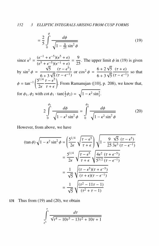
152 3 ELLIPTIC INTEGRALS ARISING FROM CUSP FORMS

=2

5

φ∫

0

dφ√

1 − 925

sin2 φ

(19)

since κ2 =(ǫ−1 + ǫ−5)(ǫ5 + ǫ)

(ǫ5 + ǫ−5)(ǫ−1 + ǫ)=

9

25. The upper limit φ in (19) is given

by sin2 φ =

√5

6 + 3√

5

(τ − ǫ5)

(τ − ǫ−1)or cos2 φ =

6 + 2√

5

6 + 3√

5

(τ + ǫ)

(τ − ǫ−1)so that

φ = tan−1

(

51/4

2ǫ

τ − ǫ5

τ + ǫ

)

. From Ramanujan ([10], p. 208), we know that,

for φ1, φ2 with cot φ1 · tan(12φ2) =

√

1 − κ2 sin21.

2

φ1∫

0

dφ√

1 − κ2 sin2 φ

=

φ2∫

0

dφ√

1 − κ2 sin2 φ

(20)

However, from above, we have

(tan φ)

√

1 − κ2 sin2 φ =

51/4

2ǫ

√

τ − ǫ5

τ + ǫ

√

1 − 9

25

√5

3ǫ3

(τ − ǫ5)

(τ − ǫ−1)

=51/4

2ǫ

√

τ − ǫ5

τ + ǫ

√

4ǫ2

53/2

(τ + ǫ−5)

(τ − ǫ−1)

=1√

5

√

(τ − ǫ5)(τ + ǫ−5)

(τ + ǫ)(τ − ǫ−1)

=1√

5

√

(τ2 − 11τ − 1)

(τ2 + τ − 1)

Thus from (19) and (20), we obtain131

τ∫

ǫ5

dτ√τ4 − 10τ3 − 13τ2 + 10τ + 1

3.1 153

=1

5

2 tan−1

(

1√5

√

(τ2−11τ−1)

(τ2+τ−1)

)

∫

0

dφ√

1 − 925

sin2 φ

=1

5

2 tan−1(

1√5

√

1−11v−v2

1+v−v2

)

∫

0

dφ√

1 − 925

sin2 φ

where v =1

τ=η3η3

15

η33η3

5

. Hence

∞∫

τ

dτ√τ4 − · · · + 1

=

∞∫

ǫ5

dτ√τ4 − · · · + 1

−τ

∫

ǫ5

dτ√τ4 − · · · + 1

=1

5

2 tan−1(1/√

5)∫

0

dφ√

1 − 925

sin2 φ

−1

5

2 tan−10

(

1√

1−11v−v2

√5 1+v−v2

)

∫

dφ√

1 − 925

sin2 φ

=1

5

2 tan−1

(

15

√(1−11v−v2)

1+v−v2

)

∫

2 tan−1(1/√

5)

dφ√

1 − 925

sin2 φ

which together with (18) gives us Ramanujan’s formula (??).

The right hand side of (??) admits of interesting reduction when

one resorts to well-known transformations available for elliptic integrals 132

such as Landen’s transformation or Gauss’ transformation. On page 67

154 3 ELLIPTIC INTEGRALS ARISING FROM CUSP FORMS

+ 1 of [11], Ramanujan also notes that

=1

5

2 tan−1(1/√

5)∫

2 tan−1

1√5

√

(1−11v−v2)

1+v−v2

dφ√

1 − 925

sin2 φ

=1

9

π/2∫

2 tan−1

(

(1−v/ǫ3)

(1+vǫ3)

√

(1+vǫ)(1−vǫ5)

(1−v/ǫ)(1+v/ǫ5)

)

dψ√

1 − 181

sin2 ψ

(21)

also equal to

1

4

tan−1(3−√

5)∫

tan−1

(

(3−√

5)

√

(1−v/ǫ)(1−vǫ5)

(1−vǫ)(1+v/ǫ5)

)

dψ√

1 − 1516

sin2 ψ

(22)

with v and ǫ as above.

To prove (21), let us use Landen’s transformation ([12], p. 496) :∫

dφ√

1 − κ2 sin2 φ

=1

1 +√

1 − κ2

∫

dψ√

1 −(

1−√

1−κ2

1+√

1−κ2

)2

sin2 ψ

for tan(ψ − φ) − (√

1 − κ2) tan φ (23)

with κ = 3/5 and determine the limits of integration on the right hand

side corresponding to those on the left hand side of (23). We have only

to verify that the relations

tan(ψ − φ) =4

5tan φ, tan(φ/2) =

1√

5

√

1 − 11v − v2

1 + v − v2

together imply that

tan(ψ/2) =1 − v/ǫ3

1 + vǫ3

√

(1 + vǫ)(1 − vǫ5)

(1 − v/ǫ)(1 + v/ǫ5),

3.1 155

so that the upper limit π/2 for ψ in (21) will correspond to 2 tan−1(1/√

5)

arising for v = 0. Setting t1 = tan(φ/2), t2 = tan((ψ − φ)/2), we have

then2t2

1 − t22

= tan(ψ − φ) =4

5

2t1

1 − t21

and so 133

t2 =5(1 − t2

1)

4t1± 1

2

√

√

25

16

(1 − t21)2

t21

+ 4.

Since 1−t21= 1−(1−11v−v2)/[5(1+v−v2)] = (4/5)(1+4v−v2)/(1+v−v2)

and (25/16)(1 − t21)2/t2

1+ 4 = 9(1 + v2)2/(1 + v − v2) × (1 − 11v − v2),

we have

t2 =−√

5(1 + 4v − v2) + 3(1 + v2)

2√

(1 + v − v2)(1 − 11v − v2)

noting that only the positive root has to be taken for t2, in view of t2having to be positive for large v. Thus

t2 =ǫ2(ǫ − v)(ǫ−5 − v)

√

(1 − v/ǫ)(1 + vǫ)(1 − vǫ5)(1 + v/ǫ5)

= ǫ−2

√

(1 − v/ǫ)(1 − vǫ5)

(1 + vǫ)(1 + v/ǫ5).

Finally

tan(ψ/2) =t1 + t2

1 − t1t2=

1√5

√

1−11v−v2

1+v−v2 1 + v − v2 + ǫ−2√

(1−v/ǫ)(1−vǫ5)

(1+vǫ)(1+v/ǫ5)

1 − ǫ−2√

5

(1−vǫ5)(1+vǫ)

=

√

(1−vǫ5)

(1−v/ǫ)(1+vǫ)(1+v/ǫ5 )

1/(1 + vǫ)·

(1 + v/ǫ5) +√

5ǫ−2(1 − v/ǫ)√

5(1 + vǫ) − ǫ−2(1 − vǫ5)

=

√

(1 − vǫ5)(1 + vǫ)

(1 − v/ǫ)(1 + v/ǫ5)· (1 − vǫ−3)

(1 + vǫ3)

establishing the validity of (21).

156 3 ELLIPTIC INTEGRALS ARISING FROM CUSP FORMS

In order to prove (22), apply Gauss’ transformation [12] :∫

dφ√

1 − κ2 sin2 φ

=2

1 + κ

∫

dψ√

1 − [4κ/(1 + κ)2] sin2 ψ

for sin(2ψ − φ) = κ sin φ

with κ = 3/5 again and determine the limits of integration which corre-134

spond to each other on either side. From sin(2ψ − φ) = (3/5) sin φ, we

get a quadratic equation for t := tanψ, viz.

5t

4 − t2= tan φ =

2 tan φ/2

1 − tan2(φ/2)=

√5

2

√

(1 − 11v − v2)(1 + v − v2)

(1 + 4v − v2)

proceeding as in the earlier case. Since by the same calculations,

20(1 + 4v − v2)2

(1 − 11v − v2)(1 + v − v2)+ 16 =

36(1 + v2)2

(1 − 11v − v2)(1 + v − v2),

we get

tanψ = t =−√

5(1 + 4v − v2) + 3(1 + v2)√

(1 − 11v − v2)(1 + v − v2)

taking the positive square root as before. Thus

t =2

ǫ2

√

(1 − v/ǫ)(1 − vǫ5)

(1 + vǫ)(1 + v/ǫ5)

giving the lower limit for ψ in (22); the upper limit tan−1(3−√

5) clearly

corresponds to the upper limit 2 tan−1(1/√

5) arising when v = 0. Con-

sequently Ramanujan’s formula (22) is proved.

Using a different ‘uniformiser’ v1 :=η2(3z)η2(15z)

η2(z)η2(5z)related to Γ0(15),

Ramanujan ([11], p. 70/78) also records the formula :

x∫

0

ηη3η5η15

dx

x=

1

5

2 tan−1(1/√

5)∫

2 tan−1(1 − 3v1)√

5(1 + 3v1)

√

dφ

√

1 −9

25sin2 φ (24)

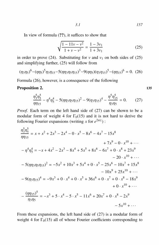
3.1 157

In view of formula (??), it suffices to show that

√

1 − 11v − v2

1 + v − v2=

1 − 3v1

1 + 3v1

(25)

in order to prove (24). Substituting for v and v1 on both sides of (25)

and simplifying further, (25) will follow from

(η3η5)6−(ηη5)5η3η15−5(ηη3η5η15)3−9(ηη5)(η3η15)5−(ηη15)6 = 0. (26)

Formula (26), however, is a consequence of the following

Proposition 2. 135

η53η5

5

ηη15

− η4η45 − 5(ηη3η5η15)2 − 9(η3η15)4 −

η5η515

η3η5

= 0. (27)

Proof. Each term on the left hand side of (27) can be shown to be a

modular form of weight 4 for Γ0(15) and it is not hard to derive the

following Fourier expansions (writing x for e2πiz) :

η53η5

5

ηη15

= x + x2 + 2x3 − 2x4 − 0 · x5 − 8x6 − 4x7 − 15x8

+ 7x9 − 0 · x10 + · · ·− η4η4

5 = −x + 4x2 − 2x3 − 8x4 + 5x5 + 8x6 − 6x7 + 0 · x8 + 23x9

− 20 · x10 + · · ·− 5(ηη3η5η15)2 = −5x2 + 10x3 + 5x4 + 0 · x5 − 25x6 − 10x7 + 15x8

− 10x9 + 25x10 + · · ·− 9(η3η15)4 = −9x3 + 0 · x4 + 0 · x5 + 36x6 + 0 · x7 + 0 · x8 − 18x9

+ 0 · x10 + · · ·

−(ηη15)5

η3η5

= −x3 + 5 · x4 − 5 · x5 − 11x6 + 20x7 + 0 · x8 − 2x9

− 5x10 + · · ·

From these expansions, the left hand side of (27) is a modular form of

weight 4 for Γ0(15) all of whose Fourier coefficients corresponding to

158 3 ELLIPTIC INTEGRALS ARISING FROM CUSP FORMS

e2πinz for 0 ≤ n ≤ 8 = 4[Γ(1) : Γ0(15)]/12 vanish. By Hecke’s theorem

([5], p. 811-see also p. 953) again, this modular form has to vanish

identically.

Remark. We may rewrite (27) in terms of the above modular functions

v, v1 for Γ0(15) as1

v− v − 5 − 9v1 −

1

v1

= 0 (28)

If we show that the left hand side (which is already regular on all of H is

also regular at all the four cusps of Γ0(15), we can obtain an alternative

proof for (27), via (28).

3.2 Ramanujan has considered on the same page 67 + 1 of [11] an

elliptic integral coming now from the group Γ0(14) of genus 1 and has

noted the formula

x∫

0

ηη2η7η14dx

x= . . .

∫

cos−1

(

17

1+v21−v2

√13+16

√2

)

dφ√

1 − 16√

2−13

32√

2sin2 φ

(29)

where v2 := (ηη14/η2η7)4.136

We know that τ := 1/v2 and σ :=2πi

4π2ηη2η7η14

dτ

dzare connected

by the relation σ2 = τ4 − 14τ3 + 19τ2 − 14τ + 1, from Fricke ([3], pp.

451-453) and in fact, they generate the field of modular functions for

Γ0(14). Proceeding as in §3.1, we have

x∫

0

ηη2η7η14

dx

x= −πi

i∞∫

z

ηη2η7η14dz (with z = iy, y > 0)

=

∞∫

τ

dτ√τ4 − 14τ3 + 19τ2 − 14τ + 1

(30)

Now X4−14X3 +19X2−14X +1 = (X−α)(X −β)[(X −m)2+n2) where

α = 12(7 + 4

√2 +√

7

√

11 + 8√

2), β = 12(7 + 4

√2 −√

7

√

11 + 8√

2),

3.2 159

m = 12(7−4

√2), n2 = 7

4(8√

2−11). From Greenhill ([4], p. 61 as quoted

from page 23 of “Elliptische Funktionen” by Enneper), we obtain

x∫

α

dX√

(X − α)(X − β)[(X − m)2 + n2)

=1√

HKcn−1

H(X − β) − K(X − α)

H(X − β) + K(X − α), κ

=1√

HK

φ∫

0

dφ√

1 − κ2 sin2 φ

with φ = cos−1

(

H(X − β) − K(X − α)

H(X − β) + K(X − α)

)

,H2 = (α−m)2 + n2 = 4√

2(7+

4√

2+√

7

√

11 + 8√

2), K2 = (β−m)2+n2 = 4√

2(7+4√

2−√

7

√

11 + 8√

2),

and κ2 = 12− 1

4(α − β)2 − H2 − K2/HK. Also, HK = 8

√2 and

κ2 = (16√

2 − 13)/(32√

2). Hence, for the (real-valued) integral (30) 137

wherein τ > α necessarily, we have the value

x∫

α

−τ

∫

α

dτ√τ4 − · · · + 1

=1

√

8√

2

cos−1( H−KH+K )

∫

cos−1

(

H−K−v2(Hβ−Kα)

H−K−v2(Hβ+Kα)

)

dφ√

1 −16√

2 − 13

32√

2sin2 φ

=1

√

8√

2

cos−1

( √13+16

√2

7

)

∫

cos−1

( √13+16

√2

7

1+v21−v2

)

dφ√

1 − 16√

2−13

32√

2sin2 φ

since H2β = K2α = HK, (Hβ−Kα)/(K −H) = 1 = (Hβ+Kα)/(H+K)

160 3 ELLIPTIC INTEGRALS ARISING FROM CUSP FORMS

and (H −K)/(H +K) = (H2 −K2)/(H2 +K2 + 2HK) = 17

√

13 + 16√

2.

This proves formula (29).

3.3 An integral of the same form as above but not of elliptic type has

been mentioned by Ramanujan on page 70 /78 of [11] :

x∫

0

ηη5η7η35

dx

x=

1

2

v3∫

0

dt√

(1 − t +√

t)(1 − t3 −√

t(5 + 9t + 5t2))

(31)

where v3 = (ηη35η5η7)2.

If τ := 1/√

v3 and σ =4πi

2π2η2η235

dτ

dz, then by Fricke ([3], pp. 444-

445), σ and τ are modular functions for Γ0(35) connected by the relation

σ2 = τ8 − 4τ7 − 6τ6 − 4τ5 − 9τ4 + 4τ3 − 6τ2 + 4τ + 1. [The right hand

side factorizes as (τ2 + τ − 1)(τ6 − 5τ5 − 9τ3 − 5τ − 1)]. As in earlier

examples,

x∫

0

ηη5η7η35dx

x=

∞∫

τ

τdτ√

(τ2 + τ − 1)(τ6 − 5τ5 − 9τ3 − 5τ − 1)

=1

2

v3∫

0

√dt

√

(1 − t +√

t)(1 − t3 −√

t(5 + 9t + 5t2))

(setting τ = 1/√

t)

138

Remarks. The further reduction of this hyperelliptic integral can be car-

ried out by known methods in the theory of elliptic functions ([4], pp.

159-160).

It is interesting to note the following relation between P = η/η7 and

Q = η5/η35 on page 303 of [10] :

(PQ)2 − 5 + 49/(PQ)2 = (Q/P)3 − 5(Q/P)2 − 5(P/Q)2 − (P/Q)3

3.4 161

which is the same as equation (29) on page 446 of Fricke (3); the latter

is itself a consequence of the above relation between σ and τ.

3.4 Ramanujan has also considered elliptic integrals wherein the inte-

grand involves (higher) powers of η. On page 45 /54 of [11], he has

written down the following formulae :

53/4

x∫

0

η2η25

dx

x=

2 tan−1(53/4√λk)

∫

0

dφ√

1 − ǫ−55−3/2 sin2 φ

(32)

= 2

π/2∫

cos−1[(ǫu)5/2]

dφ√

1 − ǫ−55−3/2 sin2 φ

(33)

=√

5

2 tan−1[51/4√

xψ(x5)/ψ(x)]∫

0

dφ√

1 − ǫ/√

5) sin2 φ

(34)

recalling that λ5 = n65/η6, u =

x1/5

1+

x

1+

x2

1+. . ., ψ(x) = x−1/8 × η2

2(z)/η(z)

and ǫ = (√

5 + 1)/2.

Before proving (32)–(34), we state

Proposition 3.

(i) E2(z) − 5E2(5z) = −4(η5/η5)

√

1 + 22λ5 + 125λ25

(ii) E4(z) = η10/η25+ 250η4η4

5+ 3125η10

5/η2

(iii) E4(5z) = η10/η25+ 10η4η4

5+ 5η10

5/η2.

Proof. We know that η10/η25, η4η4

5, η10

5/η2 form a basis for the space of

modular forms of Haupttypus (−4, 5, 1) and their Fourier expansions are

given by

η10/η25 = 1 − 10e2πiz + 35e4πiz + · · ·

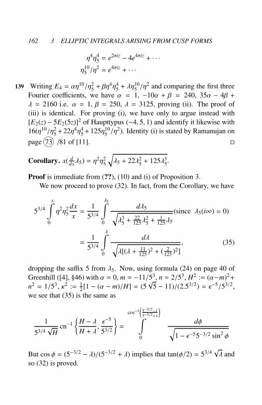
162 3 ELLIPTIC INTEGRALS ARISING FROM CUSP FORMS

η4η45 = e2πiz − 4e4πiz + · · ·

η105 /η

2 = e4πiz + · · ·

Writing E4 = αη10/η2

5+ βη4η4

5+ λη10

5/η2 and comparing the first three139

Fourier coefficients, we have α = 1, −10α + β = 240, 35α − 4β +

λ = 2160 i.e. α = 1, β = 250, λ = 3125, proving (ii). The proof of

(iii) is identical. For proving (i), we have only to argue instead with

[E2(z) − 5E2(5z)]2 of Haupttypus (−4, 5, 1) and identify it likewise with

16(η10/η25+22η4η4

5+125η10

5/η2). Identity (i) is stated by Ramanujan on

page 73 /81 of [11].

Corollary. x( ddxλ5) = η2η2

5

√

λ5 + 22λ25+ 125λ3

5.

Proof is immediate from (??), (10) and (i) of Proposition 3.

We now proceed to prove (32). In fact, from the Corollary, we have

53/4

x∫

0

η2η25

dx

x=

1

53/4

λ5∫

0

dλ5√

λ35+ 22

125λ2

5+ 1

125λ5

(since λ5(i∞) = 0)

=1

53/4

λ∫

0

dλ√

λ[(λ + 11125

)2 + ( 2125

)2]

, (35)

dropping the suffix 5 from λ5. Now, using formula (24) on page 40 of

Greenhill ([4], §46) with α = 0, m = −11/53, n = 2/53, H2 := (α−m)2+

n2 = 1/53, κ2 := 12[1 − (α − m)/H] = (5

√5 − 11)/(2.53/2) = ǫ−5/53/2,

we see that (35) is the same as

1

53/4√

Hcn−1

H − λH + λ

,ǫ−5

53/2

=

cos−1(

5−3/2−λ5−3/2+λ

)

∫

0

dφ√

1 − ǫ−55−3/2 sin2 φ

But cos φ = (5−3/2 − λ)/(5−3/2 + λ) implies that tan(φ/2) = 53/4√λ and

so (32) is proved.

3.4 163

To prove that the right hand side of (32) is the same as (33), let

us first invoke the following transformation formulae from Ramanujan

([10], Chapter XVII, 7(vi) and 7(ii), pp. 207-208) :

β∫

0

dφ√

1 − κ2 sin2 φ

= 2

α∫

0

dφ√

1 − κ2 sin2 φ

(where tan(β/2) = (tan α)|√

1 − κ2 sin2 α)

= 2

λ∫

0

dφ√

1 − κ2 cos2 φ

(where tan λ = (tan α)√

1 − κ2)

which together imply that 140

β∫

0

dφ√

1 − κ2 sin2 φ

= 2

π/2∫

π/2−λ

dφ√

1 − κ2 sin2 φ

(36)

Now taking

κ2 = ǫ−5/53/2 and λ = (π/2) − cos−1((ǫu)5/2),

we have

tan λ = (ǫu)5/2/

√

1 − (ǫu)5,

tanα = (tan λ)/√

1 − κ2 = 53/4u5/2/

√

1 − (ǫu)5,

1 − κ2 sin2 α = 1/(1 + ǫ−5u5)

and

tan(β/2) = (tan α)√

1 − κ2 sin2 α

= 53/4u5/2/

√

(1 − ǫ5u5)(1 + ǫ−5u5)

164 3 ELLIPTIC INTEGRALS ARISING FROM CUSP FORMS

= 53/4/√

u−5 − u5 − 11 = 53/4√

λ5,

by (3). Our assertion above concerning (32) and (33) is immediate.

Finally, we show that the right hand side of (32) coincides with (34).

For this, we need to use Ramanujan’s transformation formula ([10], p.

231 – see also Smith [12], p. 469) :

A∫

0

dφ√

1 − κ2 sin2 φ

=3

1 + 2α

B∫

0

dφ√

1 − µ2 sin2 φ

(37)

where κ2 =α3(2 + α)

1 + 2α, µ2 = α

(

2 + α

1 + 2a

)3

and

tan((A − B)/2) = (1 − α)/(2α + 1) tan B. (38)

Taking α = 1/(ǫ2√

5), we have 1 − α = 3/(ǫ√

5), 2α + 1 = 3/√

5,

2 + α = 3ǫ/√

5, κ2 = ǫ−5/53/2 and µ2 = ǫ/√

5. Further, in (37), if we

take A = 2 tan−1(53/4√λ5)B = 2 tan−1[51/4

√xψ(x5)/ψ(x)], we have to

verify that (38) holds. But the latter is the same as

η35

η3=ηη2

10

η22η5

×1 − (ηη2

10/η2

2η5)2

1 − 5(ηη210/η2

2η5)2

which, on the other hand, follows at once from Proposition 1. It is now

clear that (37) implies our assertion concerning (32) and (34).

Remark. On the same page in [11] wherein Ramanujan has noted down

formulae (32)-(34) as well as the integrals in (39)-(41) considered in

§3.5, one finds also values of κ2, κ2(1−κ2) corresponding to two succes-

sive “cubic” transformations. We should mention here that classically141

the object of applying such transformations to elliptic integrals repeat-

edly was the realisation of the complete integral in the limit ([4], p. 322).

3.5 Formulae (32)-(34) were connected with the modular relation (3)

for u. The following formulae due to Ramanujan ([11], p. 45 /54) are

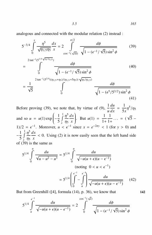
3.5 165

analogous and connected with the modular relation (2) instead :

5−3/4

x∫

0

η5

√η1/5η5

dx

x= 2

π/2∫

cos−1(√

su)

dφ√

1 − (ǫ−1/√

5) sin2 φ

(39)

=

2 tan−1(51/4√η5/η1/5 )

∫

0

dφ√

1 − (ǫ−1/√

5) sin2 φ

(40)

=1√

5

2 tan−1(53/4((η1/5+η5)/(η1/5+5η5))√η5/η1/5)

∫

0

dφ√

1 − (ǫ5/53/2) sin2 φ

(41)

Before proving (39), we note that, by virtue of (9),1

u

du

dx=

1

5xη5/η5

and so u = u(1) exp

−1

5

1∫

x

η5

η5

dx

x

. But u(1) =1

1+

1

1+. . . = (

√5 −

1)/2 = ǫ−1. Moreover, u < ǫ−1 since x = e−2πy < 1 (for y > 0) and

−1

5

1∫

x

η5

η5

dx

x< 0. Using (2) it is now easily seen that the left hand side

of (39) is the same as

51/4

u∫

0

du√

u − u2 − u3= 51/4

u∫

0

du√

−u(u + ǫ)(u − ǫ−1)

(noting 0 < u < ǫ−1)

= 51/4

ǫ−1∫

0

−ǫ−1∫

u

du√

−u(u + ǫ)(u − ǫ−1)(42)

But from Greenhill ([4], formula (14), p. 36), we know that 142

51/4

ǫ−1∫

u

du√

−u(u + ǫ)(u − ǫ−1)= 2

cos−1(√ǫ)

∫

0

dφ√

1 − (ǫ−1/√

5) sin2 φ

166 3 ELLIPTIC INTEGRALS ARISING FROM CUSP FORMS

taking M = 12(ǫ−1 + ǫ)1/2 and (κ′)2 = ǫ−1/(ǫ + ǫ−1) = ǫ−1/

√5 therein.

Letting u tend to 0 in (??) and substituting into (42), we see that formula

(39) is true.

In order to verify that (40) is the same as the right hand side of

(39), we have only to use Ramanujan’s formula (36) with κ2 = ǫ−1/√

5

and λ = π2− cos−1(

√ǫu); indeed, tan λ = (ǫu/(1 − ǫu))1/2, tan2 α =√

5 u/(1 − ǫu), 1 − (ǫ−1/√

5) sin2 α = 1/(1 + ǫ−1u) and consequently

tan β/2 = (ǫu/(1− ǫu))1/251/4/(ǫ+u)1/2 = 51/4(η5η/η1/5) in view of (2).

For proving that (40) and (41) are the same, we appeal to the Leg-

endre transformation ([4], p. 323) :

∞∫

0

dφ√

1 − κ2 sin2 φ

=1

2α + 1

ψ∫

0

dψ√

1 − µ2 sin2 ψ

(with tanφ + ψ

2= (α + 1) tan φ)

where κ2 = (α4 + 2α3)/(2α+ 1) and µ2 = α[(α+ 2)/(2α + 1)]3; we need

only to take α = ǫ−1, φ = 2 tan−1(51/4 √η1/5η5) and ψ = 2 tan−1(53/4 ·√

η5/η1/5 · [(η1/5 + η5)/(η1/5 + 5η5)] and verify that tanφ + ψ

2= (α +

1) tan φ.

3.6 Finally, we take up an interesting formula stated by Ramanujan

([11], p. 45 /54) concerning u, namely

u−5 + u5 =η3

2η35

C +

1∫

x

η8

η45

dx

x+ 125

x∫

x

η85

η4

dx

x

(44)

where

C = 53/4

−π + 4

π/2∫

0

√

1 − ǫ−55−3/2 sin2 φ dφ−

3.6 167

π/2∫

0

√

dφ

√

1 − ǫ−55−3/2 sin2 φ

143

To prove (44), we first remark that G := 2√λ5(u5 + u−5) is the same

as 2√

125λ5 + 22 + 1/λ5, in view of the modular relation (3). Hence

dG

dx=

125 − 1/λ25√

125λ5 + 22 + 1/λ5

dλk

dx

=1

x

125η8

5

η4−η8

η45

, by Corollary to Proposition 3.

Now, by the fundamental theorem of the integral calculus,

G(x) −G(e−2π/θ) =

x∫

e−2π/θ

125η8

5

η4

dx

x−

x∫

e−2π/θ

η8

η45

dx

x(for any θ > 0)

Consequently, we have

u−5 + u5 =η3

2η35

C′ +

1∫

x

η8

η45

dx

x+ 125

x∫

0

η85

η4

dx

x

(45)

where

C′ := G(e−2π/θ) − 125

e−2π/θ∫

0

η85

η4

dx

x−

1∫

e−2π/θ

η8

η45

dx

x.

It is easy to see that C′ is independent of θ and moreover C′ < G(e−2π/θ)

for all θ > 0. From the transformation formula for the η-function, we

find that

125 ·η6(− 1

z)

η6(− 15z

)=η6(z)

η65(z)

(46)

125 ·η8

5

η4

(

− 1

5z

)

= 5 · (z/i)2 · η8(z)

η45(z)

168 3 ELLIPTIC INTEGRALS ARISING FROM CUSP FORMS

and therefore

125

e−2π/θ∫

0

η85

η4

dx

x=

1∫

e−2πθ/5

η8

η45

dx

x·(

using z→ −1

5z

)

.

As a result,

C′ = G(e−2π/θ) − 250

e−2π/θ∫

0

η85

η4

dx

x= G(e−2π/θ) − 2

1∫

e−2πθ/5

η8

η45

dx

x.

Formula (45) may now be rewritten as144

u−5 + u5 =η3

2η35

C +

e−2π/θ∫

x

η8

η45

dx

x+ 125

x∫

e−2π/θ

η85

η4

dx

x

,

denoting

C′ +

1∫

e−2π/θ

η8

η45

dx

x+ 125

e−2π/θ∫

0

η85

η4

dx

x(= G(e−2π/θ) clearly) by C.

This last stated formula for u−5 + u5 may be deemed to be obtained

from (45), merely by replacing the limits of integration 0, 1 therein by

e−2π/θ and further the constant of integration C′ there by C(= G(e−2π/θ)).

Ramanujan evaluates the constant C for θ = 1,√

5 and 5. Taking θ =√

5

first, we obtain from (46) with z = i/√

5, that 125λ5(−1/(5i/√

5)) =

1/λ5(i/√

5), i.e. λ5(i/√

5) = 5−3/2. Hence

C = G(e−2π/√

5) = 2(125 · 5−3/2 + 22 + 53/2)1/2 = 4(11 + 5√

5)/2)1/2,

in agreement with Ramanujan’s value for C for this case. Again, us-

ing the functional equation for λ5 implied by (46) with z = i, we have

125λ5(i) = 1/λ5(i/5) and therefore G(e−2π) = G(e−2π/5). From Ra-

manujan’s identity (iii) in §4, viz.

E26 = η

24(η3/η35 − 500η3

5/η3 − 56 · η9

5/η9)2(1 + 22λ5 + 125λ2

5),

169

we infer λ5(i) is a root of the polynomial 1 − 500X − 15625X2 since

E6(i) = 0 and the polynomial 1 + 22X + 125X2 has no real root. Thus

λ5(i) = 1/(5ǫ)3 and consequently, G(e−2π/5) = G(e−2π) = 6·51/4(3+√

5);

however, this does not agree with the value for C given by Ramanujan.

Remark. It is possible to express C′ in terms of complete elliptic inte-

grals of the first and the second kind as Ramanujan has noted in connec-

tion with C in (44).

4 Identities for Eisenstein series We discuss in this sec-

tion several useful identities for E4(z), E4(pz), E6(z) and E6(pz) for

p = 5, 7 written down by Ramanujan ([11], p. 70 /78, also p. 67

/75) :

(i) E34(z) = (η10/η2

5+ 250η4η4

5+ 55 · η10

5/η2)3

(ii) E34(5z) = (η10/η2

5+ 10η4η4

5+ 5η10

5/η2)3

(iii) E26(z) = η24(η3/η3

5−500η3

5/η3−56η9

5/η9)2(1+22η6

5/η6+125η12

5/η12)

(iv) E26(5z) = η24

5(η15/η15

5+4η9/η9

5−η3/η3

5)2(1+22η6

5/η6+125η12

5/η12)

145

(v) E34(z) = (η7/η7 + 5 · 72η3η3

7+ 74η7

7/η)3(η7/η7 + 13η3η3

7+ 49η7

7/η)

(vi) E34(7z) = (η7/η7 + 5η3η3

7+ η7

7/η)3(η7/η7 + 13η3η3

7+ 49η7

7/η)

(vii) E26(z) = (η7/η7 − 72(5 + 2

√7)η3η3

7− 73(21 + 8

√7)η7

7/η)2×

(η7/η7 − 72(5 − 2√

7)η3η37− 73(21 − 8

√7)η7/η)2

(viii) E26(7z) = (η7/η7 − (7 + 2

√7)η3η3

7+ (21 + 8

√7η7

7/η)2×

(η7/η7 − (7 − 2√

7)η3η37+ (21 − 8

√7)η7

7/η)2

Identities (i) and (ii) have already been proved as (ii) and (iii) in

Proposition 2 in §3.4. One can derive the other identities in a similar

fashion. We can also deduce these identities from the results of Klein

([7], p. 46). If τ1 := −λ−15

and τ2 := λ−17

, then for elliptic modular

function j(z), we have from Klein (see also [4], p. 329) the following

relations :

1705 DIFFERENTIAL EQUATIONS SATISFIED BY ‘EISENSTEIN SERIES’

(i) 1728 j(z) = (τ21− 250τ1 + 55)3/(−τ5

1)

(ii) 1728 j(5z) = (τ21− 10τ1 + 5)3/(−τ1)

(iii) 1728( j(z) − 1) = (τ21+ 500τ1 − 56)2(τ2

1− 22τ1 + 125)/(−(τ5

1))

(iv) 1728( j(5z) − 1) = (τ21− 4τ1 − 1)2(τ2

1− 22τ1 + 125)/(−τ1)

(v) 1728 j(z) = (τ22+ 5 · 72τ2 + 74)3(τ2 + 13τ2 + 49)/τ7

2

(vi) 1728 j(7z) = (τ22+ 5τ2 + 1)3(τ2

2+ 13τ2 + 49)/τ2

(vii) 1728[ j(z) − 1) = (τ42= 10 · 72τ3

2− 9 · 74τ2

2− 2 · 76τ2 − 77)2/τ7

2

(viii) 1728( j(7z) − 1) = (τ42+ 14 · τ3

2+ 9 · 7τ2

2+ 10 · 7τ2 − 7)2/τ2

Substituting for j(z) = E34/(E3

4− E2

6) = E3

4/(1728 η24), we deduce Ra-

manujan’s identities (i)-(viii) immediately from the above identities (i)-

(viii).

One finds a few more striking identities involving the Eisenstein se-

ries E4 and E6, stated by Ramanujan ([11], p. 67 + 1) :

(E24(z) + 94E4(z)E4(5z) + 625E2

4(5z))1/2

= 12√

5(η10/η25 + 26η4η4

5 + 125η105 /η

2) (47)

(5(E6(z) + 125E6(5z))2 − (126)2E6(z)E6(5z))1/2 (48)

= 252(η10/η25 + 62η4η4

5 + 125η105 /η

2)(η10/η25 + 22η4η4

5 + 125η104 /η

2)1/2

Identity (47) may be verified by squaring both sides, substituting

the expressions for E4(z) and E4(5z) from the identities (i)-(ii) above

and checking that the coefficients corresponding to the monomials η24,

η18η65, η12η12

5, η6η18

5and η24

5are the same on both sides. A similar remark

applies to identity (48), using now identities (iii)-(iv) for E6 above.

171

5 Differential equations satisfied by ‘Eisenstein se-ries’ We discuss, in this section, a differential equation mentioned

by Ramanujan ([11], p. 73 /81) for certain ‘Eisenstein series’. First,146

let us recall ‘Hecke summation’ ([5], p. 469) for Eisenstem series of

weight 2 :

Lts→0

∑

(c,d)=1c≥0

(cz + d)−2 |cz + d|−s

=−6i

π(z − z)+ 1 − 24

∞∑

n=1

∑

0<d|nd

e2πinz

=−6i

π(z − z)+ E2(z) (49)

The left hand side of (49) picks up a factor of automorphy of weight

2 under modular substitutions but is not holomorphic in z, due to the

presence of −6i/(π(z − z)) on the right hand side; on the other hand,

E2 is holomorphic but it does not have a nice behaviour under modular

transformations. Now associated with E2(z) and E2(5z), Ramanujan has

introduced on page 73 /81 of [11] a function F through the equations

E2(z) = (η5/η5)[(1 + 22λ5 + 125λ25)1/2 − 30F(λ5)]

E2(5z) = (η5/η5)[(1 + 22λ5 + 125λ25)1/2 − 6F(λ5)] (50)

These two equations for F are certainly consistent by virtue of (i) in

Proposition 3 above; further, they clearly imply that

F(λ5) = −(1/24)(η5/η5)(E2(z) − E2(5z))

= −(η5/η5)E5(z) (51)

on defining E5(z) = (E2(z) − E2(5z))/24. For F(λ5), Ramanujan ([11],

p. 73 ) has recorded the non-linear differential equation.

(1 + 22λ5 + 125λ25)1/2

(

d

dλ5

F

)

= 1 + (25/2)λ5 + [5/(2λ5)]F2(λ5). (52)

1725 DIFFERENTIAL EQUATIONS SATISFIED BY ‘EISENSTEIN SERIES’

This differential equation may be verified by using the relation E4 =

E22− 12ϑ(E2) from (1) and the identity (i) above, namely

E4 = g25(1 + 250λ5 + 3125λ2

5) = g25(h5(λ5) + 228λ5 + 3000λ2

5)

with

g5 := η5/η5 and h5(X) := 1 + 22X + 125X2.

In fact, by (50), E22= g2

5(h5(λ5) − 60

√h5(λ5)F + 900F2) and further

ϑ(E2) = g25(−5√

h5(λ5)F+150F2+11λ5+125λ25−30λ5

√h5(λ5) d

dλ5F) on

noting that ϑλ5 = g5λ5

√h5(λ5) in view of the Corollary to Proposition

3. Now F = −E5/g5 and logarithmic differentiation with respect to z

gives (ϑF)/F = (ϑE5)/E5 − (ϑg5)/g5 = (ϑE5)/E5 + 5g5F, by (8) and

(50). This enables us to rewrite (52) as a differential equation for E5 :

ϑE5 −5

2E

25 = −η

4η45 −

25

2η10

5 /η2. (53)

The right hand side can be expressed as a linear combination of E4(z),147

E4(5z) and η4η45

which form a basis for the space of modular forms of

Haupttypus (−4, 5, 1).

Remark. The differential equation (53) for E5 is perhaps the right ana-

logue of the first relation in (1), for the case of Γ0(5). We derive next an

analogue for the case of Γ0(7) as follows.

Let us start from Ramanujan’s identity (v) above for E4, namely

E4 = g7(1 + 5 · 72λ7 + 74λ27)(g7 · h7(λ7))1/3 (54)

where g7 := η7/η7 and h7(X) := 1 + 13X + 49X2. We might men-

tion here that (g7 · h7(λ7))1/3 is just the Eisenstein series E1(z;χ7) =

1+2∞∑

n=1χ7(n)×xn/(1−xn) of weight 1 and (real) Nebentypus (−1, 7, χ7);

further E21(z, χ7) happens to be precisely −(1/6)E2(z; 1;Γ0(7)). By anal-

ogy with Ramanujan’s function F(λ5) above, let us introduce F1 =

F1(λ7) by the two equations

E2(z) = g2/3

7((7/6)F1(λ7) + h

2/3

7(λ7))

173

E2(7z) = g2/3

7((1/6)F1(λ7) + h

2/3

7(λ7)) (55)

The consistency of (55) follows from the relation

E2(z; 1;Γ0(7)) + 6E21(z;χ7) = 0.

In view of (8), we have

F1(λ7) = g−2/3

7(E2(z) − E2(7z)) = (12/7πi)g

−2/3

7

d

dz(log g7).

Moreover, by (10), (??) and (55).

(1/λ7)

(

d

dzλ7

)

= (2πi/6)(7E2(7z) − E2(z)) = 2πig2/37

h2/37

(λ7).

Now (1), (54) and (55) together imply that

g4/37

h1/37

(λ7)(1 + 5 · 72λ7 + 74 · λ27)

= g4/3

7((49/36)F2

1 + (7/3)F1 · h2/3

7(λ7)+

h4/37

(λ7)) − 12ϑE2 and

(

d

dzE2

)

= (2/3)g−1/37

(

d

dzg7

) (

7

6F1 + h

2/37

(λ7)

)

+

g2/3

7

(

d

dzλ7

) (

7

6F′1(λ7) +

2

3h−1/3

7(λ7)(13 + 98λ7)

)

.

Consequently, we obtain the differential equation

F′1(λ7)h1/37

(λ7) + [7/(72λ7)]h−1/37

F21(λ7) + 224λ7 + 24 = 0.

Defining E7 by E7 = (1/24)g2/37

F1, we see that

(1/E7)dE7

dz= [F1(λ7)/F1(λ7)]

dλ7

dz+ (2/3)

d

dz(log g7)

= −2πiλ7 g2/3

7× h

1/3

7(λ7) × [(7/72λ7)]h

−1/3

7(λ7)

F1 + (224λ7 + 24)/F1) + (28πi/3)E7

174 REFERENCES

= (14πi/3)E7 − (2πi/3)(3 + 28λ7)λ7g4/3

7h

1/3

7(λ7)/E7.

This leads at once to a differential equation for E7 (analogous to (53)) :

ϑE7 −7

3E

2

7= −1

3(3λ7 + 28λ2

7)g4/37

h1/37

(λ7)

= −1

3(3λ7g7 + 28λ2

7g7)E1(z;χ7)

= −η3η37E1(z;χ7) − (28/3)(η7

7/η)E1(z;χ7).

The right hand side, being a modular form of weight 4 for Γ0(7) is ex-148

pressible as a linear combination of E4(z), E4(7z) and (ηη7)3E1(z;χ7);

note that by Ramanujan’s identities (v), (vi) above, E1(z;χ7) divides

E4(z) and E4(7z) and hence every modular form of Haupttypus (−4, 7, 1).

Remark. Eichler and Zagier [2] have obtained for the N-divisor values

of Weierstrass’ ℘-function a non-linear differential equation of degree 2

with the coefficients independent of N. Eisenstein series of weight 2 for

Γ(N) are known to be expressible linearly in terms of these Weierstrass’

N-divisor values. For the ‘Eisenstein series’ E5, E7 which are analogues

of E2 for Γ0(5), Γ0(7) respectively, we have again a non-linear differ-

ential equation whose coefficients however depend on the stufe. In any

case, it is remarkable that Ramanujan has recorded in [11] the interest-

ing differential equation (52) for F(λ5) which is the same as (53) and

which does not seem to have been observed prior to Ramanujan.

References

[1] B. C. Berndt : Chapter 19 of Ramanujan’s second notebook

(Preprint).

[2] M. Eichler and D. Zagier : On the zeros of the Weierstrass ℘-

function, Math. Annalen 258 (1982), 399-407.

[3] R. Fricke : Die Elliptische Funktionen und ihre Anwendungen, Bd.

II, B. G. Teubner Verlag, 1922.

REFERENCES 175

[4] A. G. Greenhill : The Applications of Elliptic Functions, Dover

Publications Inc., New York.

[5] E. Hecke : Gesammelte Abhandlungen, Vandenhoeck und

Ruprecht, Gottingen.

[6] G. H. Hardy : Ramanujan, Chelsea Publishing Company, New

York.

[7] F. Klein : Gesammelte Abhandlungen, Vol. III, Springer-Verlag. 149

[8] S. Raghavan : On certain identities due to Ramanujan, Quart. J.

Math. Oxford (2), 37(1986) 221-229.

[9] S. Ramanujan : Collected Papers, Cambridge University Press.

[10] S. Ramanujan : Notebooks of Srinivasa Ramanujan, Vol. II, Tata

Institute of Fundamental Research, Bombay.

[11] S. Ramanujan : “Lost Notebook” (Manuscript with Trinity College

Library, Cambridge), The Lost Notebook and Other Unpublished

Papers, Narosa Publishing House, New Delhi.

[12] H. J. S. Smith : Collected Papers, Vol. II, Chelsea Publishing Com-

pany, New York.

[13] G. N. Watson : Proof of certain identities in combinatory analysis,

Jour. Indian Math. Soc. 20 (1933), 57-69.

[14] H. Weber : lehrbuch der Algebra, Bd. III, Chelsea Publishing

Company, New York.

School of Mathematics

Tata Institute of Fundamental Research

Homi Bhabha Road

Bombay 400 005 (India)

ON SOME THEOREMS STATED BY

RAMANUJAN

By K. G. Ramanathan

1 Ramanujan seems to have been fascinated by the continued frac-151

tions

R(τ) =e2πiτ/5

1+

e2πiτ

1+

e4πiτ

1+(1)

and

S (τ) =eπiτ/5

1−eπiτ

1+

e2πiτ

1−(2)

where τ = x + iy, y > 0, i =√−1. We discusses them in many places in

the Notebooks and more importantly in the ‘Lost’ Notebook. In partic-

ular, he evaluated R(τ) and S (τ) for τ = i√

n for many rational values of

n > 0. Some of these evaluations were sent by him to Hardy in his early

letters from India. A number of evaluations of R(τ) and S (τ) contained

in the ‘Lost’ Notebook were discussed and upheld by us [4] using the

Kronecker limit formula which seems to be well adapted for these prob-

lems. We do not, of course, know Ramanujan’s methods. They could

not be the method using the limit formula. There are two evaluations [7,

p. 46] which are particularly intriguing. The are

S (i√

3) =(−3 +

√5) +

√

6(5 +√

5)

4(3)R

S (i/√

3) =−3 +

√5 +

√

6(5 −√

5)

4(4)R

176

177

As far as we know, these two results have not been proved until now.

In attempting to prove these, we encountered another of Ramanujan’s

evaluations. If λn for integers n ≥ 1 is defined by

λn =e(π/2)

√n/3

3√

3(1 + e−π

√n/3)(1 − e−2π

√n/3)(1 − e−4π

√n/3) . . .6

the Ramanujan states

λ1 = 1, λ9 = 3, λ17 = 4 +√

17, λ25 = (2 +√

5)2,

λ33 = 18 + 3√

33, λ41 = 32 + 5√

41,

λ49 = 55 + 12√

21, λ89 = 500 + 53√

89, . . .(5)R

The function λn seems to have been introduced earlier in the Notebooks 152

(Vol 2, p. 393) where Ramanujan gives a formula for evaluating λn forn3= 11, 19, 43, 67, 163 and others. It is to be noticed that these values of

− n3

are precisely the discriminates ≡ 5(mod 8) of imaginary quadratic

fields of class number one. If we use Dedekind’s modular form

η(τ) = eπiτ/12∞∏

n=1

(1 − e2nπiτ).

then

λn =1

3√

3

η[12(1 + i

√n/3)]

η[12(1 + i

√3n)]

6

(6)

As was shown by us in [5], if −3n is a fundamental discriminant of an

imaginary quadratic field K = Q(√−3n) which has only one class in

each genus of ideal classes, then λn can be evaluated fairly easily using

L-series. For example, for n = 17, 41, 89 this property is true. How-

ever, for n = 25, 49 the numbers −3.25 and −3.49 are not fundamental

discriminant of an imaginary quadratic field K = Q(√−3n) which has

only one class in each genus of ideal classes, then λn can be evaluated

fairly easily using L-series. For example, for n = 17, 41, 89 this prop-

erty is true. However, for n = 25, 49 the numbers −3.25 and −3.49 are

not fundamental discriminants but nevertheless they are discriminants in

178 2

the orders in Q(√−3) with conductors 5 and 7, with similar properties

with regard to genera of ring ideal classes. One has then an analogue of

the Kronecker limit formula for the L-series of such ideal classes which

leads to the evaluation of λ25 and λ49 and consequently to the proof of

(3) and (4). For n = 9 and 33, the subrings of Q(√−3) and Q(

√−11)

with conductors 3 have similar properties but the evaluation of λ9 and

λ33 depends on different ideas.

Ramanujan, in every case, seems to consider only dicriminants, fun-

damental or not, which have only two classes. We shall do the same in

this note and restrict further to odd discriminants with class number 2

since we are dealing only with S (τ).

2 Let K = Q(√

d), d < 0 be an imaginary quadratic field with dis-

criminant d and class number h(d). Let R be the maximal order in K

and for any rational integer f ≥ 1, R f the ring with conductor f . Clearly

R = R1. The ring R f has discriminant d f 2 and a minimal basis (1, θ)

where

θ =

−1+i√

D f 2

2, if d f 2 ≡ 1(mod 4)

i√

D f 2

2, if d f 2 ≡ 0(mod 4)

(7)

where D = |d|.153

We consider in R f only ideals which are prime to f . As is well

known, there is a (1, 1) correspondence between ideals in R prime to f

and those in R f prime to f . If a and b are two ideals prime to f , in R f ,

then they are said to be in the same ideal class in R f if there exist λ and

µ in R f both prime to f such that

λa = µb

This leads to a class division of ideals of R f into ideal classes. The

number h(d f 2) of these ideal classes is given by

h(d f 2) =h(d) · ϕ([ f ])

e · ϕ( f )(8)

179

where ϕ([ f ]) denotes the Euler function of the ideal [ f ] in R so that

ϕ([ f ]) = f 2∏

κ/ f

(1 − 1

Nκ) (9)

where κ runs through all prime ideals in R dividing f and ϕ( f ) in the

denominator is the ordinary totient function. The number e is the index

of the group of units in R f in the group of units of R.

It is to be noted that formula (8) is still true if d > 0.

Let C be any ideal class in R f . The zeta function ζ∗f(s,C) of the class

C is defined by

ζ∗f (S ,C) =∑

a∈C(a, f )=1

(Na)−s, Re s > 1 (10)

where a runs through all integral ideals in C which are prime to f . If ℓ

is an ideal in the class C−1 which is prime to f , then

ζ∗f (s,C) =(Nℓ)s

w

∑

0,α∈ℓ(α, f )=1

|Nα|−s (11)

w being the number of roots of unity in R f . If f > 1, then w = 2.

If f > 1, because of the restrictive summation in (11), it is not

possible to apply at once the Kronecker Limit formula to ζ∗f(s,C). We

shall see that for our purposes, the zeta function of the class C in the

extended sense defined below would be sufficient. Put

ζ f (s,C) =(Nℓ)s

w

∑

α,0α∈ℓ

|Nα|−s (12)

with α running through all elements of ℓ not equal to zero. The sum in 154

(12) is then an Epstein zeta function.

We shall choose the ideal class C in a particular way using the (1, 1)

correspondence between ring ideal classes and binary, positive, primi-

tive integral quadratic forms with discriminant d f 2, d being, of course,

a negative fundamental discriminant.

180 2

Let p be a prime number dividing d but not f (we assume that

such primes exist). We shall construct a binary, primitive, positive form

which represents p primitively. Let

px2+ bxy + cy2

be the quadratic form with discriminant d f 2 so that

b2 − 4pc = d f 2. (13)

Clearly p|b and so if b = pb1, d = pd1, then

pb21 − 4c = d1 f 2.

Let p be odd. If d f 2 is odd, then

p − d1 f 2 ≡ 0(mod 4)

and so we choose b1 = 1 and

c = (p − d1 f 2)/4.

The quadratic form

px2+ pxy +

p − d1 f 2

4y2

is primitive since p ∤ d1 and is odd. It has discriminant d f 2. We choose

the ideals class C to be the inverse of the ideal class C−1 represented by

the ideal ℓ with basis (1, z) where

z =−1 +

√

d f 2/p

2(14)

The ideal clearly has norm equal to 1/p. Note that (p, f ) = 1.

If p is odd and d f 2 is even, then, by (13), 2p|b1. One easily sees that

we can again take the quadratic form to be

px2+ 2pxy + (p − d1 f 2/4)y2

181

which means that the ideal class C−1 is represented by the ideal (1, z)

with

z =

√

d f 2/2p (15)

In a similar way, we obtain for C−1 the ideal class represented by the

ideal (1, z) with

z =

12(1 +

√

d f 2/2) , p = 2, (d/4) odd√

d f 2/4 , p = 2, (d/4) even(16)

If we go back to formula (12) and take C = C0 as the principal class and 155

apply the Kronecker limit formula ([5, formula 6]), we have

− lims→1

[ζ f (s,C0) − ζ f (s,C) =

= (4π/w√

D f 2) log(N[1, z])1/2 |η(z)/η(θ)|2)(17)

where w = w f is the number of roots of unity in R f , z is given by (14),

(15) and (16) and θ by (7). The two functions ζ f (s,C0) and ζ f (s,C) are

the zeta functions of the classes C0 and C respectively in the extended

sense.

3 In order to proceed further, it is necessary to obtain another expres-

sion for the left side of (17).

Let χ be any character of the ring ideal class group of R f . We define

the L-function

L f (s, χ) =∑

a∈R f

(a, f1)=1

χ(a)

(Na)s, Re s > 1. (18)

since χ is a multiplicative function on the ideal of R f prime to f .

L f (s, χ) =∏

κ| f(1 − χ(κ)Nκ−s)−1 (19)

Furthermore

L f (s, χ) =∑

C

χ(C)ζ∗f (s,C) (20)

182 3

where C runs through all ring ideal classes of R f .

If χ is a non-principal character, it is shown by Meyer that we have

even the relation

L f (s, χ) =∑

C

χ(C)ζ f (s,C) (21)

in terms of the zeta functions of classes in the extended sense. Formula

(21) has the advantage that one can apply the Kronecker limit formula.

If now we assume that every genus of ring ideal classes of R f has only

one class in it, then one has

− 2r−2

ζ f (s,C0) − ζ f (s,C) =∑

χ(c)=−1

L(s, χ)

(22)

where the sum runs through all characters which take the value −1 on

C, 2r−1 being the number of genera.

We now define the genus characters.

Let d f 2 have the decomposition

d f 2= d0d∗0

where d0 is a fundamental discriminant and d∗0

a discriminant. For such156

a decomposition, we have a character of the class group of R f

χd0(κ) =

(

d0

Nκ

)

for all prime ideals κwhich do not divide d f 2;

(

d0

)

being the Kronecker

symbol ([9, p. 380 et seq]). For prime ideals not dividing d0, (??) also

makes sense. If κ divides d0, then take

χd0(κ) =

(

d∗0

Nκ

)

It is to be noted that d0 and d∗0

have only divisors of f as common divisor.

We shall now confine ourselves to the case

d f 2 odd, h(d f 2) = 2, (d, f ) = 1. (23)

183

Since d is a fundamental discriminant,

d f 2= −p f 2, p ≡ −1(mod 4) (24)

Further d f 2 has only one non-trivial decomposition

d f 2=

−p f · f , if f ≡ 1(mod 4)

− f · p f , if f ≡ −1(mod 4)(25)

Following Siegel [8], we see that there is only one L-series and

L f (s, χ) =

L−p f (s) · L f (s), if f ≡ 1(mod 4)

L− f (s) · Lp f (s), if f ≡ −1(mod 4)

where L∗(s) is the ordinary Dirichlet L series.

From (22), we get

− lims→1

(ζ f (s,C0) − ζ f (s,C)) = L f (1, χ)

and therefore, from (17) using the fact that w = 2 for f > 1, we get

1√

p

η

(

−1+i√

f 2/p

2

)

η

(

−1+i√

f 2 p

2

)

2

=

(ǫ( f )h(−p f )·h( f ) , f ≡ 1(mod 4)

(ǫ(p f )h(p f )·h(− f )·2/w0 , f ≡ −1(mod 4)

where h(−p f ), . . . are class numbers, ǫ( f ) and ǫ(p f ) are the fundamental

units in the real quadratic fields Q(√

f ) and Q(√

p f ) respectively and

w0 the number of roots of unity in Q(√

− f ).

From the definition of λn and formula (??), we see that we can eval-

uate λn if p = 3 and the conditions (23) are satisfied.

They are indeed satisfied in cases

d f 2= −3 · 52,−3 · 72

as seen from the tables in [1]. In case p = 3, f = 5, we have 157

184 3

ǫ( f ) = (√

5 + 1)/2 and h(−15) = 2.

We therefore have

λ25 =1

3√

3,

η

(

−1+i√

25/32

)

η

(

−1+i√

752

)

6

=

√5 + 1

2

6

= (2 +√

5)2 (5)R

In a similar way, if p = 3, f = 7, h(21) = 1, ǫ(21) = (5 +√

21)/2. This

gives since w0 = 2,

λ49 =

5 +√

21

2

3

= 55 + 12√

21. (5)R

The value of λ25 enables us to prove Ramanujan’s statements (??) and

(??). It is known, by taking τ = i√

3 in ([4, p. 700]) that

[S (i√

3)]−1+ 1 − S (i

√3) =

η(i√

3/5)

η(i5√

3)· f (i√

3/5)

f (i5√

3)(26)

where f (τ) is Schlefli’s modular function

f (τ) = e−πi/24 · η((1 + η)/2)

η(η)= f (−1/τ) (27)

If we use the formula

η(−1/τ) = (−iτ)1/2η(τ) (28)

Then

η(i√

3/5) f (i√

3/5)

η(i5√

3) f (i5√

3)=

(

5√

3

)1/2η[(1 + i

√25/3)/2]

η(1 + i√

75/2)

so that, by definition of λ25,

[S (i√

3)]−1+ 1 − S (i

√3) =

√5 − λ1/6

25=

√5(√

5 + 1)/2

185

Solving the above quadratic equation for S (i√

3) and using the fact that

S (i√

3) > 0, we get

S (i√

3) =−(3 +

√5) +

√

6(5 +√

5)

4(3)R

The value of S (i/√

3) can be obtained by again using (27) and (28) or

by using the formula

S (τ) +

√5 − 1

2

S (−1/τ) +

√5 − 1

2

=

√5

√5 − 1

2

(29)

which was stated by Ramanujan in his Notebooks. It was first proved 158

by Watson. (See also [4]).

If we use the formulae (29) and

(S (τ))5+

√5 − 1

2

5

+

(

(S (−1/5τ)5+

( √5−12

)5)

= 5√

5

√5 − 1

2

5(30)

proved by us, one can obtain the values of S [i5k(√

3)1] where k is any

rational integer and 1 = ±1.

4 We shall prove now the other statements of Ramanujan in (??).

In the first place,

λ1 =1

3√

3

η(i/√

3)

η(i√

3)· f (i/

√3)

f (i√

3)

6

.

If we now use the formulae (27) and (28) we get

λ1 = 1

Consider now λ9. By definition,

λ9 =1

3√

3

η((1 + i√

3)/2)

η((1 + i3√

3)/2)

6

186 4

If we use the product expansion of the η-function, then

λ9 =−i

3√

3

(

η(ω)

η(3ω)

)6

, ω =−1 + i

√3

2. (31)

On the other hand,

α = 27

(

η(3ω)

η(ω)

)6

is a root of the equation

x4+ 18x2

+ λ3(ω)χ − 27 = 0

where

λ3(ω) =√

j(ω) − 1728

and j(ω) is the well-known Klein’s invariant ([9, p. 504]). Weber has

shown that

λ3((−1 + i√

3)/2) = i.24√

3

and therefore λ = λ9 is a root, positive, of159

x4 − 8x3+ 18x2 − 27 = 0.

This however equals

(x + 1)(x − 3)3

which shows that

λ9 = 3 (5)R

Consider now ω = (1 + i√

11)/2. Then

λ33 =−i

3√

3

(

η(ω)

η(3ω)

)6

=3√

3i

α

where

= 27 ·

η(3(−1 + i√

11)/2)

η((−1 + i√

11)/2)

6

REFERENCES 187

From Weber [9, p. 504],

λ3

−1 + i√

11

2

= 56i√

11

and hence λ is the positive root of

9x4 − 56√

33x3+ 18 · 32 · x2 − 35

= 0 (32)

This quartic equation can be solved by the classical methods of the the-

ory of algebraic equations. One obtains

λ = λ33 = 3(6 +√

33).

In fact, Weber (loc. cit) has given the values of λ3((−1+ i√

n)/2) for

n = 19, 43, 67 and 163 and thus λ3n is a root of a quadratic equation like

(32) from which λ3n can be evaluated.

References

[1] Z. I. Borevich and I. R. Shafarevich : Number Theory, Academic

Press, New York (1966).

[2] R. Fricke : Die elliptische Funktionen und ihre Anwendungen, Bd

II, B.G. Teubner, Berlin (1922).

[3] C. Meyer : Die Berechnung der Klassenzahl abelscher Korper 160

uber quadratischen Zahlkorpern, Akademie Verlag, Berlin (1957).

[4] K. G. Ramanathan : Ramanujan’s continued fraction, Indian Jour.

Pure Appl. Math., 16(1985), 695-724.

[5] K. G. Ramanathan : Some applications of Kronecker’s limit for-

mula, Jour. Ind. Math. Soc., 52(1987), 71-89.

[6] S. Ramanujan : Notebooks, Vol. 2, Tata Institute of Fundamental

Research, Bombay (1957).

188 REFERENCES

[7] S. Ramanujan : The Lost Notebook and other unpublished papers,

Narosa Publishing House, New Delhi (1987).

[8] C. L. Siegel : Analytische Zahlentheorie II, Gottingen (1963).

[9] H. Weber : Lehrbuch der Algebra, Bd. III, Braunschweig (1908).

A1 Sri Krishna Dham

70, L. B. S. Marg

Mulund (West)

Bombay 400 080

THE ADJOINT HECKE OPERATOR II

By R. A. Rankin

161

1 Introduction Progress on the theory of modular forms and as-

sociated Euler products can be divided roughly into three stages. At the

first fundamental stage there is the work of Hecke [3], who introduced

the linear operators Tn now associated with his name. The second stage

comprises the work of Petersson [8], who observed that the space M of

cusp forms of given level, weight and character is a finite-dimensional

Hilbert space, and showed that the adjoint Hecke operator T ∗n is a scalar

multiple of Tn, provided that n is a prime to the level N of M. The

foundations of the third stage were laid by Atkin and Lehner [1], who

separated off from M the subspace M− consisting essentially of forms

of lower level, and concentrated their attention on its orthogonal com-

plement M+, showing by delicate methods that M+ has an orthogonal

basis of forms that are eigenforms for all the operators Tn and not only

for those with n prime to N.

The present paper arose from an effort to simplify the arguments of

the third stage, by investigating the properties of the adjoint operator

T ∗n for all n, and showing, if possible, that it commutes with Tn on the

subspace M+. We recall that, for any forms f and g in M, T ∗n is defined

by

( f |Tn, g) = ( f , g|T ∗n ). (1.1)

Petersson proved that T ∗n = χ(n)Tn if (N, n) = 1, where χ is the associ-

ated Dirichlet character. For this he provided two proofs. Of these one

[8] was fairly direct, but had a combinatorial part in which a common

left and right transversal of a certain group was shown to exist (Hilfs-

satz 2), and did not seem applicable to other values of n. On the other

hand, his other earlier proof [7] (p. 68), although only valid when the

189

190 2 GROUPS, MATRICES AND CHARACTERS

weight k of the space exceeds 2, seemed more promising, although tech-

nically somewhat complicated, as it involved the evaluation of G|Tn for

an arbitrary Poincare series G in M.

This is the method developed in my first paper under the same title

[10], where is yielded an apparently previously unknown explicit defi-

nition of T ∗n for (n,N) , 1. The case when N is a prime number was

then investigated in detail using properties of Poincare series. However,

for composite N this method becomes decidedly more complicated, be-

cause of increased number of incongruent cusps of verying cusp widths

and parameters. In the present paper the general case is considered in a162

relatively simple way without the use of Poincare series, and the explicit

definition of the adjoint operator, found in [10], is proved by a different

method.

2 Groups, matrices and characters As is customary, we

write

Γ(1) := SL(2,Z) (2.1)

for the modular group and, for any positive real number m, we denote

by Ωm the set of all matrices

T :=

[

a b

c d

]

(2.2)

belonging to GL(2,R) and having determinant m. We shall be particu-

larly concerned with the group

Γ0(N) = T ∈ Γ(1) : c ≡ 0(mod N), (2.3)

where N is a positive integer, and require the following special matrices

in Γ(1) :

I =

[

1 0

0 1

]

, U =

[

1 1

0 1

]

, V =

[

0 −1

1 0

]

, W =

[

1 0

1 1

]

. (2.4)

Write also

Γ(N) = T ∈ Γ(1) : T ≡ I(mod N). (2.5)

191

For various positive rational values of m we write

Jm =

[

1 0

0 m

]

. (2.6)

Throughout k will be a positive integer and, for typographical rea-

sons we write

K =1

2k − 1. (2.7)

Let

H = z ∈ C : Imz > 0, (2.8)

and put, as customary,

e(z) = exp(2πiz) (z ∈ C). (2.9)

For T ∈ Ωm, we define

Tz :=az + b

cz + d, T : z = cz + d. (2.10)

For any function f : H→ C and T ∈ Ωm(m > 0) we define

f (z)|T := (T : z)−k(det T )k/2 f (Tz). (2.11)

This depends of course on k, which is fixed. Note that

f (z)|Jm = m−k/2 f (z/m), f (z)|J−1m = mk/2 f (mz). (2.12)

The letters p and q will always denote prime numbers, and we write

P = 0, 1, . . . , p − 1, P∗ = 1, 2, . . . , q − 1, (2.13)

Q = 0, 1, . . . , q − 1, Q∗ = 1, 2, . . . , q − 1. (2.14)

Throughout, χ denotes a character modulo N such that 163

χ(−1) = (−1)k; (2.15)

it follows that, when k is odd, N ≥ 3. We denote by N(χ) the conductor

of χ and put

n(χ) = N/N(χ). (2.16)

192 3 M(N,K, χ) AND ITS SUBSPACES

Note that, for any positive integer r,

r|n(χ) ⇔ N(χ)|(N/r). (2.17)

The principal character modulo m is denoted by ǫm.

Accordingly, χ may be written as

χ = χ∗ǫN , (2.18)

where χ∗ is a primitive character modulo N(χ). When (2.17) holds

χr := χ∗ǫN/r (2.19)

is a character modulo N/r with conductor χ∗.

3 M(N, k, χ) and its subspaces A standard notation for the

vector space of cusp forms belonging to a group Γ and having weight k

and multiplier system v is

Γ, k, v0 (3.1)

and we shall write

M = M(N, k, χ) = Γ0(N), k, χ0. (3.2)

Thus M is a space of level N, weight k and character χ.

For any positive integers r and s satisfying

r|n(χ), s|r (3.3)

we define

C(r, s, χr) := M(N/r, k, χr)|J−1s , (3.4)

where χr is defined by (2.19). Note that

C(1, 1, χ1) = M. (3.5)

It is easy to see that

C(r, s, χr) ⊆ M(Ns/r, k, χr/s) ⊆ M. (3.6)

193

Whenever r > 1 and s < r the level of C(r, s, χr) is less than

N. When r = s > 1 the level is N, but the space is isomorphic to

M(N/r, k, χr) and so can be regarded as a space of essentially lower

level. For this reason we define

M− =⊕

r,s

C(r, s, χr)(r > 1, r|n(x), s|r). (3.7)

Then M− is a subspace of M of essentially lower level and any mem-

ber of M− is called an oldform. Now M is a finite-dimensional Hilbert

space, and we define M+ to be the orthogonal complement of M− in M,

so that

M = M− ⊕ M+. (3.8)

The definition of M− can be simplified, as the following Theorem 164

shows.

Theorem 3.1. We have

M− =⊕

p|n(χ)

C(p, χp), (3.9)

where

C(p, χ) = C(p, 1, χp) ⊕C(p, p, χp). (3.10)

Proof. We observe that

C(rs, t, χrs) ⊆ C(r, t, χr)(t|r, rs|n(χ)) (3.11)

and

C(rs, rt, χrs) ⊆ C(s, t, χs)(t|s, rs|n(χ)) (3.12)

It is clear that (3.11) holds. To prove (3.12) take any

F ∈ C(rs, rt, χrs),

so that we can put

F = g|J−1t = f |J−1

rt ,

194 4 THE FRICKE INVOLUTION HR

where

f ∈ M(N/rs, k, χrs).

Now take any T ∈ Γ0(N/s), so that

T1 := J−1r T Jr ∈ Γ0(N/(rs)).

Then

g|T = f |J−1r T = f |T1J−1

r = χrs(T1) f |J−1r

= χrs(T1)g = χs(T )g,

so that g ∈ M(N/s, k, χs), and this proves (3.12).

By successive applications of (3.11) and (3.12) we complete the

proof of the theorem.

4 The Fricke involution Hr For any r ∈ N define

Hr = JrV =

[

0 −1

r 0

]

(4.1)

so that H2r = −rI and H−1

r = −r−1Hr. It is easily verified that

H−1r Γ0(r)Hr = HrΓ0(r)H−1

r = Γ0(r). (4.2)

Lemma 4.1. Let N = rs where r|n(χ). Then

M(N/r, k, χr)|Hs = M(N/r, k, χr). (4.3)

In particular

M(N, k, χ)|HN = M(N, k, χ). (4.4)

Further, if N = pt, where p|n(χ), then

C(p, p, χp)|HN = C(p, 1, χp) (4.5)

and

C(p, 1, χp)|HN = C(p, p, χp). (4.6)

195

Proof. Let f ∈ M(N/r, k, χr)|Hs so that f = g|Hs, where g ∈ M(N/r, k, χr).165

Take any T ∈ Γ0(N/r) so that

H−1s T Hs ∈ Γ0(s).

Then

f |T = g|T Hs = g|HsH−1s T Hs = χr(H

−1s T Hs)g|Hs

= χr(H−1s T Hs) f = χr(T ) f .

Moreover

C(p, p, χp)|HN = C(p, 1, χp)|J−1p HN = C(p, 1, χp)|Ht

= C(p, 1, χp),

by (4.4) with N replaced by t. This gives (4.5) and (4.6) follows by

replacing χ by χ and operating again on the right with HN .

Lemma 4.2. If N = pt, then

HN JpUuH−1N = pW−ut J−1

p . (4.7)

Proof. Straightforward.

5 The Hecke operators Tn For any n ∈ N and any f ∈

M(N, k, χ) define the operator Tn(N, χ) = Tn by

f |Tn = nk∑

ad=n

d∑

u=1

χ(a) f |JdUuJ−1a , (5.1)

where J is given by (2.7), and observe that, for any prime p we have, in

particular,

f |Tp = pK

∑

u∈P

f |JpUu+ χ(p) f |J−1

p

; (5.2)

196 5 THE HECKE OPERATORS TN

see (2.12). It is clear that, in (5.2), u can run through any complete set

of residues modulo p.

If

N = pt, p ∤ t and f ∈ C(p, 1, χp), (5.3)

if follows from (5.2) that

f |Tp(t, χp) = f |Tp(N, χ) + pKχp(p) f |J−1p (5.4)

and we note that χp(p) , 0 in this case.

We now summarize some of the known properties of the operators.

For any f ∈ M, let

f (z) =

∞∑

r=1

a(r)e(rz). (5.5)

Then166

f (z)|Tn =

∞∑

r=1

an(r)e(rz), (5.6)

where

an(r) =∑

d|(n,r)

dk−1χ(d)a(nr/d2). (5.7)

Moreover, we have

M|Tn ⊂ M (n ∈ N) (5.8)

and

( f |Tm)|Tn =

∑

d|(m,n)

dk−1χ(d) f |Tmn/d2 (m ∈ N, n ∈ N). (5.9)

It follows that the operators commute and that Tn is completely deter-

mined when Tp is known for each prime p|n.

Moreover, as shown in Petersson [8], if f and g belong to M, then

( f |Tn, g) = χ(n)( f , g|Tn) for (n,N) = 1. (5.10)

Here the inner product is defined for cusp forms f and g of weight k on

a subgroup Γ of finite index h in Γ(1) by

( f , g) = ( f , g;Γ) =1

h

"

F

f (z)g(z)yk−2dxdy. (5.11)

197

where x = Re z, y = Im z and F is any fundamental region in H for Γ.

In §6 we shall require this definition for various subgroups Γ contained

in Γ(1). It follows from (5.10) that T ∗n , the adjoint operator, is given by

T ∗n = χ(n)Tn for (n,N) = 1. (5.12)

6 The adjoint operator T ∗p for p|N For any prime p|N and

f ∈ M define the operator T ∗p = T ∗p(N, χ) by

f |T ∗p : = f |HNTpH−1N = f |H−1

N TpHN (6.1)

= pK∑

u∈P

f |HN JpUuH−1N

= pK∑

u∈P

f |W−ut J−1p (6.2)

by Lemma 4.2.

Since Tp(N, χ) = Tp(N, χ) it follows from (4.4) that

M|T ∗p ⊆ M. (6.3)

Theorem 6.1. For any prime p|N, T ∗p is the adjoint operator to Tp; i.e.

( f |T ∗p, g) = ( f , g|Tp) for f and g in M. (6.4)

For the proof we require the following Lemma, which we quote from

Theorem 5.2.1 of [9].

Lemma 6.2. (i) If Γ1 and Γ2 are subgroups of Γ(1) of finite index in Γ(1) 167

and Γ1 ⊆ Γ2, then

( f , g : Γ1) = ( f , g : Γ2)

whenever f and g both belong to Γ2, k, v0.

198 6 THE ADJOINT OPERATOR T ∗P

FOR P|N

(ii) Let Γ be a congruence subgroup of Γ(1) of finite index and let, for

any prime p,

Γp = Γ ∩ Γ(p). (6.5)

Suppose that f and g belong to Γ, k, v0 and let L ∈ Ωp. Then

( f , g;Γ) = ( f |L, g|L; L−1ΓpL). (6.6)

Proof of Theorem. Take any f and g in M and write

F = f |T ∗p,

so that f ∈ M by (6.3). Note that, if S ∈ Γ(pN), then

f |W−ut J−1p S = f |S ′W−ut J−1

p ,

where S ′ ∈ Γ(N), so that χ(S ′) = 1. Hence, for any u ∈ Z,

f |W−ut J−1p ∈ Γ(pN), k, 10,

and so, by Lemma 6.2(i) and (6.2),

(F, g : Γ0(N)) = (F, g;Γ(pn)) = pK∑

u∈P

( f |W−ut J−1P , g;Γ(pN))

= pK∑

u∈P

( f |U−uW−ut J−1P , g;Γ(pN)).

Write

Au = JpWutUu= WuN JpUu ∈ Ωp

and note that, when Γ = Γ(pN),

Γp = Γ(pN),

by (6.5), so that

A−1u ΓpAu = J−1

p Γ(pN)Jp ⊇ Γ(pN2).

199

Taking L = Au in (6.6), we get

(F, g;Γ0(N)) = pK∑

u∈p

( f , g|Au;Γ(pN2))

= pK

f ,∑

u∈P

g|WuN JpUu;Γ(pN2)

= pK

f ,∑

u∈P

g|JpUu; Γ(pN2)

= ( f , g|Tp; Γ(pN2))

= ( f , g|Tp; Γ0(N)).

This completes the proof of the theorem.

Theorem 6.3. Let m and n be positive integers. Then the following pairs 168

of operators on M commute :

(i) Tm, Tn; (ii) T ∗m, T ∗n ; (iii) Tm, T ∗n provided that (m, n,N) = 1.

Proof. (i) follows from (5.9) and this yields (ii), since

( f |T ∗mT ∗n , g) = ( f , g|TnTm).

By (5.12) and (i) we need only prove that T ∗p and Tq commute when p

and q are different primes dividing N.

Write N = pqs and define S u,w by

S u,wJqUupW−wqs J−1p = W−wq2sJ−1

p JqUu

for (u,w) ∈ Q × P. Then it is easy to see that S u,w ∈ Γ0(N) and that

χ(S u,w) = 1. Now, if f ∈ M, since up and wq run through complete sets

of residues modulo p and modulo q respectively, we have

f |T ∗pTq = (pq)K∑

u∈Q

∑

w∈P

f |W−wq2s J−1p JqUu

= (pq)K∑

w∈P

∑

u∈Q

f |JqUupW−wqsJ−1p

= f |TqT ∗p.

200 7 THE ACTION OF THE OPERATORS ON M

7 The action of the operators on M

Theorem 7.1. For all n ∈ N

M−|Tn ⊆ M− · M−|T ∗n ⊂ M−. (7.1)

In particular, if p is any prime dividing N and N = pt, we have :

(i) For (n,N) = 1 and p|n(χ)

C(p, 1, χp)|Tn ⊆ C(p, 1, χp),C(p, p, χp)|Tn ⊆ C(p, p, χp). (7.2)

(ii) If p|n(χ),

C(p, p, χp)|Tp ⊆ C(p, 1, χp),C(p, 1, χp)|T ∗p ⊆ C(p, p, χp). (7.3)

(iii) If p and q are different primes dividing n(χ),

C(q, 1, χq)|Tp ⊆ C(q, 1, χq),C(q, 1, χq)|T ∗p ⊆ C(q, 1, χq), (7.4)

C(q, q, χq)|Tp ⊆ C(q, q, χq),C(q, q, χq)|T ∗p ⊆ C(q, q, χq). (7.5)

(iv) If p|n(χ) and p2|N,

C(p, 1, χp)|Tp ⊆ C(p, 1, χp),C(p, p, χp)|T ∗p ⊆ C(p, p, χp) (7.6)

(v) If p|n(χp) and p2 ∤ N.

C(p, 1, χp)|Tp ⊆ C(p, χp),C(p, p, χp)|T ∗p ⊂ C(p, χp). (7.7)

Proof. In view of Theorem 3.1, (7.1) will follow if we prove parts (i)-

(v) of the theorem. For the proof of (i) see pp. 321-322 of [9]. By (6.1),

(4.5) and (4.6) it is only necessary to prove those parts of (7.3)-(7.7) that

involve the operator Tp.

For (7.3) we note that169

C(p, p, χp)|JpUu= C(p, 1, χp)|Uu

= C(p, 1, χp).

201

For (7.4) note that the operator Tp(N, χ) is the same as the operator

Tp(N/q, χq) since p divides N/q and the latter operator maps the space

M(N/q, k, χq) into itself. Also, if N = pqs and f = g|J−1q ∈ C(q, q, χq)

then g ∈ C(q, 1, χq) and

f |Tp = pK∑

u∈P

g|J−1q JpUu

= pK∑

u=P

g|JpUuqJ−1q

= g|Tp J−1q ⊆ C(p, 1, χq)|J−1

q = C(q, q, χq).

which proves (7.5).

(7.6) follows for the same reason as (7.4), since p divides N/p and

the operators Tp(N, χ) and Tp(N/p, χp) are identical.

Finally, assume that p|n(χ) but p2 ∤ N. We assume (5.3) and deduce

that

f |Tp(N, χ) ∈ C(p, 1, χp) ⊕C(p, p, χp) = C(p, χp),

from (5.4).

Theorem 7.2. For all n ∈ N

M+|Tn ⊆ M+ and M+|T ∗n ⊆ M+.

Proof. Take any f ∈ M+ and g ∈ M−. Then

( f |Tn, g) = ( f , g|T ∗n ) = 0

by Theorem 7.1. Hence f |Tn ∈ M+. The proof of the second part is

similar.

Theorem 7.3. Let MH = M|HN. Then (MH)− = M−|HN .

Proof. By (4.4)

MH = M(N, k, χ),

so that (MH)− is a vector sum of the spaces C(p, 1, χp) and C(p, p, χp);

the result follows.

202 8 THE OPERATORS T ∗PTP AND TPT ∗

P(P|N)

8 The operators T ∗pTp and TpT ∗p(p|N)

Lemma 8.1. Let R be a right transversal of Γ0(N) in Γ0(t), where N =

tp, and put

R0 =

⋃

w∈P

W−wt. (8.1)

Then we may take

(i) R = R0, when p ∤ t, and

(ii) R = R0 ∪ R∗, when p ∤ t, where

R∗ = p−1JpU sW tJp =

(

(1 + st)/p s

t p

)

(8.2)

and s is chosen so that s ∈ P and st ≡ −1(mod p).

This is straightforward : note that R∗ ∈ Γ(1).170

Lemma 8.2. Let f ∈ M(N, k, χ), where p|n(χ). Then

F :=∑

R∈R

χ(R) f |R ∈ M(t, k, χp),

so that F ∈ M−.

Proof. Let the members of R be Rr(r = 1, 2, . . . , h) where h = [Γ0(t) :

Γ0(N)], and take any S ∈ Γ0(t). Then RS is also a right transversal of

Γ0(N) in Γ0(t) and so

RrS = S rR′r,

where R′r ∈ R and S r ∈ Γ0(N). Note that

χ(Rr)χ(S ) = χ(S r)χ(R′r).

Then

F|S =

h∑

r=1

χ(Rr) f |RrS =

h∑

r=1

χ(Rr) f |S rR′r

203

=

h∑

r=1

X(Rr)χ(S r) f |R′r =

h∑

r=1

χ(S )χ(R′r) f |R′r

= χ(S )F.

It follows that F ∈ M(t, k, χp) and this proves the lemma.

Lemma 8.3. Suppose that N = pt, where p|t, and that χ is a character

modulo N. Then, for some integer m ∈ P,

χ(1 + rt) = e(mr/p)(r ∈ Z). (8.3)

Moreover

m = 0 if and only if p|n(χ). (8.4)

Proof. Since

(1 + t)p ≡ 1(mod N),

χ(1 + t) = e(m/p) for some m ∈ P and (8.3) follows since

1 + rt ≡ (1 + t)r(mod p).

If p|n(χ), then N(χ)|t and so m = 0, Conversely, if N(χ) ∤ t, then

χ(n) , χ(n + t)

for some n prime to N and so, taking rn ≡ 1(mod N).

1 , χ(1 + rt),

from which it follows that m , 0, by (8.3).

We now define

δ(χ) = 0 if p ∤ n(χ); δ(χ) = 1 if p|n(χ). (8.5)

Further, for any prime p dividing N we put N = pt, as usual, and

define

α(p) =

0 if p|t, p|n(χ),

pk−2 if p ∤ t, p|n(χ),

pk−1 if p ∤ n(χ).

(8.6)

Then we have 171

204 8 THE OPERATORS T ∗PTP AND TPT ∗

P(P|N)

Theorem 8.4. Let f ∈ M(N, k, χ) and suppose that p|N. Then

f |T ∗pTp − α(p) f ∈ M−, (8.7)

and

f |TpT ∗p − α(p) f ∈ M−. (8.8)

Accordingly, if f ∈ M+, then

f |TpT ∗p = f |T ∗pTp = α(p) f . (8.9)

Proof. We write N = pt and, in the first instance, assume that p ∤ t.

Then we can write

χ = ψpψt,

where ψp and ψt are characters modulo p and modulo t, respectively.

For any integers u, v, w we write

S (u, v,w) := W−wtUuW−vt (8.10)

=

[

1 − uvt u

t(−v − w + uvwt) 1 − uwt

]

(8.11)

and, for any n ∈ P∗ we define n′ = P∗ by nn′ ≡ 1(mod p).

The finite set of ordered pairs P × P can be written as

P × P = A∗ ∪⋃

v∈P

Av (8.12)

where

A∗ = (w, u) ∈ P2 : w , 0, u = (wt)′ (8.13)

A0 = (w, u) ∈ P2 : w = 0 (8.14)

and, for v ∈ P∗

Av = (w, u) ∈ P2 : u , (vt)′, w = (ut − v′)′. (8.15)

It is easily checked that these p + 1 sets are disjoint and that their union

is P2. Note also that, for (w, u) ∈ Av(v , 0), we have S (u, v,w) ∈ Γ0(N).

205

For any f ∈ M(N, k, χ) we write

s∗ =∑

(w,u)∈A∗

f |W−wtUu, sv =

∑

(w,u)∈Av

f |W−wtUu(v ∈ P) (8.16)

so that

f |T ∗pTp = pk−2s∗ +∑

v∈P

sv.

For (w, u) ∈ A∗, we put

S w = W−wtUu(R∗)−1, (8.17)

where R∗ is defined by (8.2). Then S w ∈ Γ0(N) and

χ(S w) = χwst + (1 − wut)(1 + st)/p

= ψp(−w)ψt(p)

and so, by (8.16), 172

s∗ =∑

w∈P∗

f |S wR∗ = ψt(p)∑

w∈P∗

ψp(−w) f |R∗

= (p − 1)δ(χ)ψt(p) f |R∗, (8.18)

by (8.5), since p|n(χ) if and only if ψp is the principal character.

Clearly

s0 =

∑

w∈P∗

f |Uu= p f (8.19)

and, for v , 0,

sv =

∑

(w,u)∈Av

f |S (u, v,w)Wvt

=

∑

(w,u)∈Av

χ(1 − uvt) f |Wvt

=

∑

u∈P

χ(1 − uvt) f |Wvt=

∑

u∈P

ψp(1 − uvt) f |Wvt

206 8 THE OPERATORS T ∗PTP AND TPT ∗

P(P|N)

= δ(χ)(p − 1) f |Wvt (8.20)

Accordingly, by (8.18, 19, 20) we have

f T ∗pTp = pk−2

(p f + δ(χ)(p − 1)

∑

v∈P∗

f |Wvt+ ψt(p) f |R∗

. (8.21)

This gives

f |T ∗pTp = α(p) f for p ∤ t, p ∤ n(χ). (8.22)

If, however, p|n(χ), then ψt = χt and

f |T ∗pTp = α(p) f + pk−2(p − 1)F, (8.23)

where

F =∑

v∈P

f |Wvt+ ψt(p) f |R∗

=

∑

R∈R

χt(R) f |R. (8.24)

It follows from Lemma 8.2 that F ∈ M−.

It remains to consider the case when p|t. In this case S (w,w, u) ∈

Γ0(N) and we write

P × P =⋃

w∈P

Bw, (8.25)

where

Bw = (w, u) : u ∈ P. (8.26)

Then173

f |T ∗pTp = pk−2∑

w∈P

tw, (8.27)

where

tw =∑

(w,u)∈Bw

f |W−wtUu

=

∑

u∈P

f |S (u,w,w)Wwt

207

=

∑

u∈P

χ(1 − wut) f |Wwt (8.28)

Hence

t0 = p f . (8.29)

When w ∈ P∗, we have by Lemma 8.3 that

χ(1 − wut) = e(−mwu/p)(m ∈ P),

where m = 0 if and only if p|n(χ). Hence, by (8.5),

tw = pδ(χ) f |Wwt

and so

f |T ∗pTp = pk−1 f + δ(χ)∑

w∈P∗

f |Wwt. (8.30)

Accordingly, if p|n(χ), then

f |T ∗pTp = pk−1∑

R∈R0

f |R ∈ M− (8.31)

while, when p ∤ n(χ),

f |T ∗pTp = pk−1 f . (8.32)

Accordingly, (8.7) holds in either case.

To prove (8.8) we write f = g|HN , where g ∈ M(N, k, χ). Then

f |TpT ∗p = g|HNTpT ∗p = g|HNTpH−1N · HNT ∗P

= g|T ∗pHNT ∗p = g|T ∗pTpHN

= α(p)g + h|HN = α(p) f + h|HN

= α(p) f + h′,

say, where h ∈ M−(χ) and therefore, by Theorem 7.3. h′ ∈ M−.

It remains to prove (8.9). If f ∈ M+, then f |T ∗pTp ∈ M+ and so

f |T ∗pTp − α(p) f ∈ M+. It follows from (8.7) that

f |T ∗pTp = α(p) f .

The proof that f |TpT ∗p = α(p) f is similar. Theorem 8.4 is proved.

208 9 THE ACTION OF THE OPERATORS ON M+

Corollary 8.5. Suppose that f ∈ M+ and that, for some p|N we have 174

p|n(χ). Then, in the notation of Lemma 8.2,∑

T∈R

χ(T ) f |T = 0.

This follows from (8.24) and (8.31).

9 The action of the operators on M+ In this section we

are concerned solely with the space M+.

We recall that a linear operator on a Hilbert space is said to be nor-

mal if it commutes with its adjoint. Let F be the family of all the

operators Tn and T ∗n (n ∈ N). Then it follows from Theorems 6.3 and 8.4

that F is a family of normal operators acting on M+ and that any two

members of F commute. Now M+ is a finite-dimensional Hilbert space

and so, from a standard theorem on operators on such spaces (see pp.

267 and 291 of [2]), we deduce

Theorem 9.1. M+ has an orthogonal basis of forms, each of which is

an eigenvector for all the operators in F . Moreover, if f is such a

basis element, with Fourier expansion (5.5), we may assume that f is

primitive, i.e. that a(1) = 1, and then

f |Tn = a(n) f , f |T ∗n = a(n) f (n ∈ N). (9.1)

Further,

a(n) = χ(n)a(n) for (n,N) = 1, (9.2)

and, for any prime p dividing N,

|a(p)|2 = α(p). (9.3)

Proof. If f is an eigenvector of all the operators Tn(n ∈ N) with eigen-

value λ(n), then we have, taking r = 1 in (5.7)

λ(n)a(1) = an(1) = a(n)(n ∈ N),

which shows that a(1) , 0; by division, we may assume that a(1) = 1

and then we have λ(n) = a(n). Since T ∗n = χ(n)Tn for (n,N) = 1, (9.2)

follows and (8.9) gives (9.3).

REFERENCES 209

Each basis element is called a newform and M+ is the newform

space.

It may be noted that, from (8.6) and (9.3), the absolute value of the

eigenvalue a(p), where p divides N, emerges naturally from the proof of

Theorem 8.4. In certain cases one can determine a(p) rather than |a(p)|;

see [1], [4], [6], [9]. In this connexion I take the opportunity to correct

an error in the statement of Theorem 9.4.8 (iii) of [9], where condition

(d) should be replaced by

p ∤ t1, p ∤ (N/Nχ).

In conclusion, it may be noted that, although the paper [5] is not 175

concerned with the determination of adjoint Hecke operators, the linear

operator Cq there introduced has points of similarity with the operator

Tq + T ∗q , which is clearly normal on each of the subspaces M, M− and

M+.

References

[1] A.O.L. Atkin and J. Lehner : Hecke operators on Γ0(m), Math,

Ann. 185 (1969), 134-160.

[2] F.R. Gantmacher : Matrix theory, vol. 1. Chelsea, 1960.

[3] E. Hecke : Ueber Modulfunktionen und die Dirichletschen Reihen

mit Eulerscher Produktentwicklung I, Math. Ann. 144(1937), 1-28

Math. Ann. 114(1937), 316-351.

[4] W.C.W. Li : Newforms and functional equations, Math. Ann. 212

(1975), 285-315.

[5] W.C.W. Li : Diagonalizing modular forms, J. Algebra 99(1986),

210-231.

[6] A.P. Ogg : On the eigenvalues of Hecke operators, Math. Ann. 179

(1969). 101-108.

210 REFERENCES

[7] H. Petersson : Ueber eine Metrisierung der ganzen Modulformen,

Jber, Deutsch. Math. Verein. 49(1939), 49-75.

[8] H. Petersson : Konstruktion der samtlichen Losungen einer Rie-

mannschen Funktionalgleichung durch Dirichlet-Reihen mit Eu-

lerscher Produktentwicklung II, Math. Ann. 166 (1939), 39-64.

[9] R.A. Rankin : Modular forms and functions, Cambridge Univer-

sity Press 1977.

[10] R. A. Rankin : The adjoint Hecke operator I, J. Madras University

(to appear).

University of Glasgow

Glasgow G12 8QW

Scotland

ON ZETA FUNCTIONS ASSOCIATED

WITH SELF-DUAL HOMOGENEOUS

CONES

By Ichiro Satake

Let C be and (irreducible) self-dual homogeneous cone is a vec- 177

tor space V with a Q-structure such that the automorphism group G =

Aut(V,C ) is defined over O. Let M be a lattice in V and let Γ = g ∈G|gM = M. Then by definition the zeta function associated with C is

given by

ZC (M; s) =∑

x:Γ\C∩M

|Γx|−1N(x)−s (s ∈ C), (1)

where Γx = λ ∈ Γ|λx = x and N(x) is the “norm” of x (see 1).

The purpose of this note is to supplement our previous report [SO]

in the following points. First, in 2, we will show that, except for the case

C = Pr(R) and G is O-split (treated in [?]), the fundamental assump-

tion (2.6) in [SS] is satisfied, so that we can apply the general results of

Sato-Shintani on the zeta functions of prehomogeneous vector spaces to

our case. In §5, we will determine that poles and the residues of the zeta

functions, and, in 6, the functional equations (cf. [SO], Th. 2.3.1, 2.3.3).

These will be done including the case d is odd, which was excluded in

[SF] and [SO]. In particular, we will show that the matrix U(r)(x) giving

the functional equations is always diagonalizable.

1 Let V be a real vector space of dimension n endowed with a posi-

tive definite inner product 〈 〉. Let C be a self-dual homogeneous cone

in V , i.e. an open convex cone with vertex at 0 satisfying the following

two conditions :

211

212 1

(i) C is “self-dual”, i.e. one has

C = C∗= x ∈ V |〈x, y〉 〉0 for all y ∈ C − 0.

(ii) The automorphism group of C ,

G = Aut(V,C ) = g ∈ GL(V)|gC = C ,

is transitive on C ( denotes the connected component of the iden-

tity.)

In what follows, we assume for simplicity that C is irreducible and ex-

clude the trivial case C = R+ (the half-line of positive numbers). Then

G is (the identity connected component of) a reductive algebraic group

defined over R with R-rank r ≥ 2 and one has G = Gs × R+, where Gs

is R-simple. (For the treatment of the reducible case, see [SO].) For any

c0 ∈ C , the stabilizer K = Gc0is a maximal compact subgroup of G and178

one has G/K C . We can (hence will) assume that the base point c0

and the inner product 〈 〉 are so chosen that for g ∈ G one has gc0 = c0

if and only if tg−1= g. We further normalize 〈 〉 by 〈c0, c0〉 = r.

We set g = Lie G, k = Lie K, k = Lie K and let g = k + p be

the corresponding Cartan decomposition. As is well-known (see e.g.

[S1]), there exists a unique structure of Jordan algebra on V with the unit

element c0 such that, denoting by Tx(x ∈ V) the Jordan multiplication

y 7→ xy(y ∈ V), one has p = Tx(x ∈ V). We denote by N(x) the

reduced norm of this Jordan algebra. Then N : V → R is a polynomial

function of degree r defined over R satisfying the following conditions :

N(c0) = 1,N(gx) = det(g)r/nN(x) (g ∈ G, x ∈ V). (2)

It is then clear that χ(g) = det(g)r/n is a rational character of the alge-

braic group G.

One can find a system of mutually orthogonal primitive idempotents

ei(1 ≤ i ≤ r) such that

c0 =

r∑

i=1

ei, eie j = δi jei,

213

which we call a “primitive decomposition” of c0. Then a = Tei(1 ≤ i ≤

r)R is a maximal (abelian) subalgebra in p. It is known that the system

of R-roots (relative to a) is of type (Ar) and all the R-roots have the same

multiplicity d. One has a direct sum decomposition

V =⊕

k≤l

Vkl,

where

Vkl =

x ∈ V |ek x = x (k = l),

x ∈ V |ek x = elx =12

x (k < l),

and one has dim Vkk = 1 and dim Vkl = d(k < l). Hence one has the

relationn

r= 1 +

d

2(r − 1). (3)

We assume that there is given a O-structure on V (i.e. a O-vector

space VO in V with V = VO ⊗O R) such that G is defined over O and

c0 ∈ VO. Then, clearly, K, 〈 〉, N, χ are all defined over O. We denote

by r0 the O-rank of G. Then it can be shown that r0 is a divisor of r. So

we set δ = r/r0. The possible values of δ are as listed below.

C r d δ

Pr(R) ≥ 2 1 1 or 2 (r even)

Pr(C) ≥ 2 2 δ|rPr(H) ≥ 3 4 1

P3(O) 3 8 1

P(1, n − 1) 2 ≥ 3 1

179

2 To define the zeta function, we fix a lattice M in V compatible with

the given O-structure and let Γ be the stabilizer of M in G. Then Γ is

an arithmetic subgroup of G acting properly discontinuously on C . For

x ∈ V , we denote by Gx and Γx the stabilizers of x in G and Γ.

Let S denote the singular set x ∈ V |N(x) = 0 and put V× = V − S .

Let V×i

denote the set of all x ∈ V× with “signature” (r − i, i) (see §3).

214 2

Then one has an (open G-orbit decomposition

V× =r∐

i=0

V×i . (4)

Clearly one has V×i= −V×

r−i, V×

0= C .

For x ∈ V×O

, Gx is a reductive subgroup defined over O and Γx is

an arithmetic subgroup. We denote by µ(x) the volume of Γx\Gx with

respect to a suitably normalized Haar measure on Gx. In particular, if

x ∈ C , then Gx is compact, Γx is finite, and one has µ(x) = |Γx|−1 < ∞.

For all x ∈ V×iQ

(1 ≤ i ≤ r − 1), one has µ(x) < ∞ except for the case

r = 2, d = δ = 1. In what follows, we exclude this case, which is treated

in [Si] and [?]. For 0 ≤ i ≤ r we define a zeta function associated with

the G-orbit V×i

by

ξi(M; s) =∑

x∈Γ\M∩V×i

µ(x)|N(x)|−s, (5)

where the summation is taken over a complete set of representatives of

the Γ-orbits in M∩V×i

. Clearly one has ξi = ξr−i and ξ0(M; s) is the zeta

function ZC (M; s) associated with the self-dual homogeneous cone C .

To discuss the convergence of these zeta functions, we need

Lemma 1. Let G1= g ∈ G| det(g) = 1 and for f ∈ S (V) (the Schwartz

space) set

I( f ,M) =

∫

G1/Γ∩G1

∑

x∈M

f (gx)

d1g.

where d1g is a (suitably normalized) Haar measure on G1. Then, if180

dδ ≥ 2, the integral on the right hand side is absolutely convergent and

the map f 7→ I( f ,M) is a tempered distribution on V.

This is proved by applying Weil’s criterion ([W], p. 90, Lem. 5).

For c > 0 put

Ac = diag(t1, . . . , tr0)|ti ∈ R+,

r0∏

i=1

ti = 1, ti/ti+1 ≥ c

215

(1 ≤ i ≤ r0 − 1).

Then, since every O-root has the multiplicity dδ2, it is enough to show

that

∫

Ac

r0∏

i=1

Sup(1, t−2i )δ(1+(d/2)(δ−1)) ×

×∏

1≤i< j≤r0

Sup(1, t−1i t−1

j )dδ2(tit−1j )−dδ2

1/2r0−1∏

i=1

t−1i dti < ∞.

(See [SS], p. 166, Lem. 4.3.) Putting τi = (tit−1i+1

)1/r0 , one has for some

c1 > 0

Sup(1, t−2i ) ≤ c1

i−1∏

k=1

τ2kk ,

Sup(1, t−1t t−1

j ) ≤ c1

i−1∏

k=1

τ2kk

∏

i≤k< jk≥r0/2

τ2k−r0

k(i < j),

∏

i< j

(tit−1j )−1

=

r0−1∏

i=1

τ−i(r0−i)r0

i.

In view of these estimates, one sees that the above integral is

≤ c2

∫

Ac

r0−1∏

i=1

τi(r0−i)δvi

i

1/2 r0−1∏

i=1

t−1i dti

for some c2 > 0, where

vi =

2 − d(δi + 1) for 1 ≤ i ≤ [r0/2],

2 − d(δ(r0 − i) + 1) for [r0/2] + 1 ≤ i ≤ r0 − 1.

If dδ ≥ 2, one has vi < 0 for all 1 ≤ i ≤ r0 − 1, which proves our

assertion.

216 3

In what follows, we assume that dδ ≥ 2. Then Lemma 1 assures

that the fundamental assumption (2.6) in [SS] is satisfies, so that we can 181

apply the general results obtained there. (As we shall see in §3, the con-

dition (2.13) in [SS] is also satisfied). In particular, by [SS], Theorem 2,

(i), the Dirichlet series on the right hand side of (5) converges absolutely

for Re s > n/r and the function ξi(M; s) thus defined can be continued to

a meromorphic function on the whole complex plane. It is known that,

even in the case d = δ = 1, the Dirichlet series defining ZC (M; s) has

the same property ([?]).

3 We now consider the G-orbit decomposition of the singular set S =

V − V×. Every element x in V can be expressed in the form

x = k

r∑

v=1

αvev

with k ∈ K, αv ∈ R, (6)

where (α1, . . . , αr) is uniquely determined up to the order (indepen-

dently of the choice of the primitive decomposition ev) ([S3], Prop. 3).

We say that x is of rank ρ and of signature (ρ− i, i) if, in a suitable order

of (αv), one has α1, . . . , αi < 0, αi+1, . . . , αp > 0, αρ+1 = . . . = αr = 0.

For 0 ≤ ρ ≤ r − 1 and 0 ≤ i ≤ ρ, we set

S (ρ)= x ∈ V | rank x = ρ,

S(ρ)i= x ∈ V | sign x = (ρ − i, i).

Then it is easy to see that the G-orbit decomposition of S is given by

S =∐

0≤ρ≤r−10≤i≤ρ

S(ρ)i. (7)

Since G1 is transitive on each S(ρ)i

, (7) is also the G1-orbit decomposition

of S . Thus the condition (2.13) in [SS] is certainly satisfied.

By [SS], Lemmas 2.7 and 2.8, (i), there exists a G1-invariant mea-

sure dv(ρ)(v) on S (ρ) satisfying the relation

dv(ρ)(gv) = χ(g)sρ ,idv(ρ)(v) (g ∈ G, v ∈ S(ρ)i

) (8)

217

for some sρ,i ∈ R. To describe the measure dv(ρ) explicitly, we use the

following parametrization of S (ρ).

Set

e =

r−ρ∑

v=1

ev, e′ = c0 − e =

r∑

v=r−ρ+1

ev

and Vλ = Vλ(e) = x ∈ V |ex = λx. Writing v ∈ V in the form

v = v1 + v1/2 + v0, vλ ∈ Vλ(e),

we set 182

S (ρ)(e′) = v ∈ S (ρ)|N0(v0) , 0, (9)

where N0 denotes the norm of the Jordan subalgebra V0(e). Then S (ρ)(e′)is a Zariski open set in S (ρ) and by [S3], Lemma 1 every element v in

S (ρ)(e′) can be written uniquely in the form

v = exp(ey)v0 with y ∈ V1/2, v0 ∈ V0, (10)

where in general xy = Txy + [Tx, Ty] (Koecher’s notation).

By a well-known identity in the Jordan algebra one has for any y, y′

in V1/2(e)

[[Ty, Ty′], Te] = Ty(y′e)−y′(ye) = 0.

Hence one has [ey, ey′] = 0 (by [S3], (4)) and

exp(ey) · exp(ey′) = exp(e(y + y′)).

Therefore S (ρ)(e′) can be viewed as a principal bundle of the additive

group V1/2(e) with base space V0 = V0(e) by the action

v 7→ exp(ey)v(y ∈ V1/2(e), v ∈ S (ρ)(e′)).

It follows, that, if one puts

dµ(v) = dy · dv0 for v = exp(ey)v0, y ∈ V1/2, v0 ∈ V0,

then there exists a continuous function ϕ = ϕρ,i : V0(e) → R such

that dv(ρ)(v) = ϕ(v0)−1dµ(v). Putting g = λ1 in (8), one sees that ϕ is

homogeneous of degree ρ(1 + d2(ρ − 1)) − rsρ,i.

218 3

Not let G0 be the subgroup of G generated by exp Tx(x ∈ V0(e)).

Then the Vλ(e)′s are G0-invariant. For g0 ∈ G0, one has g0|V1(e) = id.

and N0(g0v0) = χ0(g0)N0(v0) for v0 ∈ V0(e), where χ0 is a rational

character of G0 satisfying the relation

det(g0|V0(e)) = χ0(g0)1+(d/2)(ρ−1). (11)

Lemma 2. For g0 ∈ G0, one has

det(g0|V1/2) = χ0(g0)(d/2)(r−ρ), (12)

χ(g0) = χ0(g0). (13)

Proof. Since g0e = e, one has for y ∈ V1/2

g0(ey)v0 = (etg−10 y)g0v0.

Hence g0(yv0) = (tg−10

y) · (g0v0), or

g0Tv0

tg0 = Tg0v0on V1/2(e). (*)

By [SF], Lemma 2, (i), one has det(2Tv0|V1/2) = N0(v0)d(r−ρ). Taking

the determinant of both sides of (*), one has

det(g0|V1/2)2N0(v0)d(r−ρ)= N0(g0v0)d(r−ρ),

whence follows (12). Since183

χ(g0)1+(d/2)(r−1)= det(g0) = det(g0|V1/2) · det(g0|V0),

(13) follows from (11) and (12).

By (11) and (12) one has

dµ(g0v) = d(tg−10 y) · d(g0v0)

= χ0(g0)−(d/2)(r−ρ)+1+(d/2)(ρ−1)dµ(v).

Hence by (8) and (13) one has

ϕ(g0v0) = χ0(g0)1−(d/2)(r−2ρ+1)−sρ,iϕ(v0).

219

In particular, ϕ is homogeneous of degree ρ(1− d2(r−2ρ+1)− sρ,i). Com-

bining this with what we mentioned above, we see that sρ,i =d2ρ, which

is independent of 0 ≤ i ≤ ρ, and that ϕ(v0) is given by cN(v0)1−(d/2)(r−ρ+1)

for some c > 0. We normalize dv(ρ)(v) by putting c = 2−dρ(r−ρ).Summing up, we have

Lemma 3. In the expression (10), aG1-invariant measure on S (ρ) is

given by

dv(ρ)(v) = 2−dρ(r−ρ)N0(v0)(d/2)(r−ρ+1)−1dy dv0. (14)

and one has

dv(ρ)(gv) = χ(g)(d/2)ρdv(ρ)(v) (g ∈ G, v ∈ S (ρ)). (15)

4 We set Vk = ⊕ j<kV jk(2 ≤ k ≤ r). Then every element v in S (ρ)(e′)can be written uniquely in the form

v =

r∑

k=r−ρ+1

ǫktk

(ek +

1

2x′k +

1

4x′2k(1 − ek)

), (16)

x′k ∈ Vk, tk ∈ R+, ǫk = ±1(r − ρ + 1 ≤ k ≤ r)

(see [S3], Prop. 1). In this expression, it is easy to see that

dv(ρ)(v) = 2−(d/2)ρ(2r−ρ−1)r∏

k=r−ρ+1

(t(d/2)(2k−r+ρ−1)−1

kdtk)dx′, (17)

where dx′ = Πdx′k

is the Euclidean measure on ⊕rk=r−ρ+1

Vk.

For 0 ≤ ρ ≤ r−1 and 0 ≤ i ≤ ρ, let E(r)

ρ,i denote the set of all r-tuples

ǫ = (ǫv) ∈ 0, 1,−1r such that

ǫv = 0(0 ≤ v ≤ r − ρ),= ±1(r − ρ + 1 ≤ v ≤ r),

and ♯v|ǫv = −1 = i.

For ǫ = (ǫv) ∈ E(r)

ρ,i , let S(ρ)ǫ denote the set of all v in S (ρ)(e′) of the form 184

220 4

(16) with the given (ǫv). Then clearly one has

S (ρ)(e′) ∩ S(ρ)i=

∐

ǫ∈E (r)

ρ,i

S(ρ)ǫ .

Let E (r)= ±1r, and for η = (ηk) ∈ E (r) let V×η denote the AN-orbit

of∑r

k=1 ηkek, where A = exp a and N is the unipotent subgroup of G

generated by exp(∑r

k=2 ekxk)(xk ∈ Vk). Then∐η∈E (r)

V×η is a Zariski open

subset of V×.

Proposition 1. Let 0 ≤ ρ ≤ r − 1 and 0 ≤ i ≤ ρ. Then, for f ∈C∞

0(∐

V×η ), one has

∫

S(ρ)i

f (v)dv(ρ)(v) =

ρ∏

k=1

[(2π)−(d/2)kΓ

(d

2k

)×

×∑

ǫ,η

e

(d

8N

(ρ)ǫη

) ∫

V×η

f (u)|N(u)|−(d/2)ρdu,

where the summation is taken over all ǫ ∈ E(r)

ρ,i η ∈ E (r), e(·) stands for

exp(2π√−1·) and

N(ρ)ǫη =

r∑

k=r−ρ+1

ǫk

k−1∑

l=1

η1 + ηk(k − r + ρ)

.

The proof is similar to that of [SF], (21), and we use basically the

same notation as in [SF]. Write u ∈ V in the form

u =

r∑

k=1

ξkek +

r∑

k=2

uk,

with

ξk ∈ R×, uk ∈ Vk

221

and for 1 ≤ k ≤ r set

u(k)=

k∑

j=1

ξ je j +

k∑

j=2

u j.

For a self-adjoint linear operator T on Vk and xk ∈ Vk, we write

T [xk] = 〈xk, T xk〉.

In particular, 185

u(k−1)[xk] = Tu(k−1)[xk] = 〈xk, u(k−1) xk〉.

Now, writing v ∈ S(ρ)ǫ in the form (16), one has

〈u, v〉 =r∑

k=r−ρ+1

ǫktk

(ξk +

1

2〈uk, x

′k〉 +

1

4u(k−1)[x′k]

)

(see [SF], p. 476). For λ > 0 and r − ρ + 1 ≤ k ≤ r, put

Qk = Qk(λ, ǫk, u(k−1)) = λ1Vk

−√−1

2ǫkTu(k−1) |Vk.

Then, for u ∈∐

V×η , one has

〈u, v〉 =√−1

2limλ→0

r∑

k=r−ρ+1

tk(λ − 2√−1ǫkξk +

+ Qk

x′k −√−1

2ǫkQ−1

k uk

+1

4Q−1

k [uk])

Hence, putting qk(λ) = λ − 2√−1ǫkξk +

1

4Q−1

k[uk], one has

Iǫ =

(ρ)∫

S ǫ

f (v)dv(ρ)(v)

222 4

=

∫

S(ρ)ǫ

∫

V

f (u)e(〈u, v〉)du

dv(ρ)(v)

= 2−(d/2)ρ(2r−ρ−1)∑

η∈E (r)

∫

V×η

f (u)du ×

+ limλ→0

r∑

k=r−ρ+1

∞∫

0

t(d/2)(2k−r+ρ−1)−1

ke

√−1

2tkqk(λ)

dtk ×

×∫

???????????

e

√−1

2tkQk

x′k −√−1

2ǫkQ−1

k uk

dx′k.

For u ∈ V×η , one has, in the notation of [SF], sign χk(u) = ηk(1 ≤ k ≤ r).186

Hence∫

Vk

e

√−1

2tkQk

x′k −√−1

2ǫkQ−1

k uk

dx′k = t

−(d/2)(k−1)

kdet(Qk)−1/2

→ 2d(k−1)t−(d/2)(k−1)

ke

d

8ǫk

k−1∑

l=1

ηl

|N(k−1)(u(k−1))|−d/2

(λ→ 0),

∞∫

0

t(d/2)(k−r+ρ)−1e

√−1

2tkqk(λ)

dtk

= Γ

(d

2(k − r + ρ)

)(πqk(λ))−(d/2)(k−r+ρ)

→ Γ(d

2(k − r + ρ)

)e

(d

8ǫkηk(k − r − ρ)

)(2|χk(u)|)−(d/2)(k−r+ρ)

(λ→ 0).

Moreover, one has

r∏

k=r−ρ+1

N(k−1)(u(k−1))|χk(u)|k−r+ρ= N(u)ρ.

223

Therefore, putting k′ = k − r + ρ(r − ρ + 1 ≤ k ≤ r), one has

Iǫ = 2(d/2)ρ(2r−ρ−1)∑

η∈E (r)

∫

V×η

f (u)du ×

× limλ→0

r∑

k=r−ρ+1

det(Qk)−1/2Γ

(d

2k′)

(πqk(λ))−(d/2)k′

=

ρ∏

k′=1

(2π)−(d/2)k′

Γ((d/2)k′)]

×∑

η

e

d

8

r∑

k=r−ρ+1

ǫk

∑

l<k

ηl

− ηk(k − r + ρ)

∫

V×η

f (u)|N(u)|−(d/2)ρdu,

which proves the Proposition.

5 We put

λρ =

ρ∏

k=1

[(2π)−(d/2)k

Γ

(d

2k

)]

Also, putting n(η) = ♯k|1 ≤ k ≤ r, ηk = −1 for η ∈ E (r), we set 187

E(r)

j= η ∈ E (r)|n(η) = j. Then for η ∈ E

(r)

jan easy computation shows

that

N(ρ)ǫη = (r − 2 j)ρ − 2i(r − ρ − 2p − 1) +

+

r∑

k=r−ρ+1

(1 − ǫk)

k−1∑

l=r−ρ+1

(1 − ηl) − (1 + ηk)(k − r + ρ)

,

where p = ♯k|1 ≤ k ≤ r − ρ, ηk = −1 and Σ′ indicates that the summa-

tion is taken over k (or l) ≥ r − ρ + 1.

We claim that∑ǫ∈E (r)

ρ,i

e

(d

8N

(ρ)ǫη

)depends only on i and j = n(η) and is

independent of the choice of η ∈ E(r)

j. Then the formula in Proposition

224 5

1 can be written as

∫

S(ρ)i

f (v)dv(ρ)(v) =

r∑

j=0

ri j

∫

V×j

f (u)|N(u)|−(d/2)ρdu, (19)

where

ri j = λρ∑

ǫ∈E (r)ρ,i

e

(d

8N

(ρ)ǫη

)(η ∈ E

(r)j

). (20)

When d is even, the above claim is obvious, since

e

(d

8N

(ρ)ǫη

)=

√−1(d/2)rρ(−1)(d/2)((r−ρ−1)i+ρ j) .

In this case, one has

ri j =

√−1(d/2)rρλρ · (−1)(d/2)(r−ρ−1)i

(ρ

i

)· (−1)(d/2)ρ j. (21)

Introducing a new variable y, one has the relation

ρ∑

i=0

ri jyi=

√−1(d/2)rρλρ · (−1)(d/2)ρ j(1 + (−1)(d/2)(r−ρ−1)y)ρ. (22)

When d is odd, we set

ω = (−1)ρ(−√−1)d(r−ρ−1)

Then for η ∈ E(r)

jone has

ρ∑

i=0

∑

ǫ∈E (r)

ρ,i

e

(d

8N

(ρ)ǫη

)yi= ζ′

drρ8

(−√−1)dρ j ×

×∑

i,ǫ

(−1)

∑k

(1−ǫk)/2∑l<k

(1−ηl)/2+(1+ηk )(k−r+ρ)/2(ωy)i

225

= ζdrρ8

(−√−1)dρ j

ρ∏

k′=1

(1 + (−1)

∑′l<k

(1−ηl)/2+(1+ηk)k/2ωy),

where the summation∑i,ǫ

is taken over all 0 ≤ i ≤ ρ, ǫ ∈ E(r)ρ,i . It can188

be shown that the last expression depends only on i and j. Actually,

defining ri j by (20), one obtains the relation

ρ∑

i=0

ri jyi= ζ

drρ8λρ(−

√−1)dρ j (22′)

×

(1 − ω2y2)ρ/2 (ρ even),

(1 − ω2y2)(ρ−1)/2 (1 − (−1) j(−√−1)d(r−ρ−1)y)(ρ odd).

Now, for the given Q-structure one has S(ρ)i∩ VQ , ∅ if and only if

ρ is a multiple of δ = r/r0. By the general theory of Sato-Shintani, we

know that for x ∈ S(ρ)i∩ VO the stabilizer G1

x of x in G1 is unimodular

and for a normalized Haar measure dvx on G1x one has

µ1(x) =

∫

G1x/Γx

dvx < ∞,

the normalization being made by the relation

∫

G1/Γx

f (gx)d1g = µ1(x)

∫

S(ρ)i

f (v)dv(ρ)(v) ( f ∈ C∞0 (S(ρ)i

)).

It is known furthermore that one has

κ(ρ)i

(M) =∑

x:Γ\M∩S(ρ)i

µ1(x) < ∞ (23)

([SS], Proof of Lemma 2.7). It can be shown that κ(ρ)i

(M) is a finite

sum of certain special values of the zeta functions associated with the

“rational boundary components” in S(ρ)i

.

226 6

By [SS], Theorem 2, (ii), one obtains the follows

Proposition 2. Assume that dδ ≥ 2. Then the zeta functions ξ j(M; s)(0 ≤j ≤ r) are holomorphic except for possible simple poles at s = n

r− d

2ρ

with 0 ≤ ρ ≤ r − 1, δ|ρ and

ResS= nr− d

2ρ ξ j = vol(V/M∗)

ρ∑

i=0

κ(ρ)i

(M∗)ri j, (24)

where M∗ is the dual lattice of M and κ(ρ)i

(M∗) and ri j are given by (23)189

(for M∗) and (22), ((22′)).In the case d is even, we set

R(ρ)= vol(V/M∗)λρ

√−1(d/2)rρ ·

ρ∑

i=0

(−1)(d/2)(r−ρ+1)i

(ρ

i

)κ

(ρ)i

(M∗). (25)

In particular, for ρ = 0, one has R(0)= vol(V/M∗) · µ1(0) > 0.

Lemma 4. When d ≡ 0(4) or ρ ≡ r−1(2), one has R(ρ), 0. When d ≡ 2

(4) and ρ ≡ r ≡ 1(2), one has R(ρ)= 0.

This follows immediately from the fact that κ(ρ)i

(M∗) > 0 and

κ(ρ)i

(M∗) = κ(ρ)ρ−i

(M∗).

By Proposition 2, the residue of ξ j at s = nr− d

2ρ(0 ≤ ρ ≤ r − 1, δ|ρ)

is given by (−1)(d/2)ρ jR(ρ). Hence, in particular, every ξ j(0 ≤ J ≤ r) has

a pole at s = n/r. It follows from Lemma 4 that, when d ≡ 0(4), every

ξ j has exactly r0 poles at s = nr− d

2δk(0 ≤ k ≤ r0 − 1). When d ≡ 2(4)

and r is odd, every ξ j has exactly (r0 + 1)/2 poles at the above s with

even k. When d ≡ 2(4) and r is even, one can only say that, if δ is odd,

every ξ j has at least [(r0 + 1)/2] poles.

6 By the general theory of Sato-Shintani we know that the zeta func-

tions satisfy functional equations of the following form

ξ j

(M∗;

n

r− s

)= vol(V/M)

r∏

k=1

[(2π)−s+(d/2)(k−1)Γ

(s − d

2(k − 1))

]×

(26)

227

× e

(r

4s

) r∑

i=0

ξi(M; s)ui j(s)

(0 ≤ j =≤ r),

where ui j(s) is a polynomial in e(− s2) determined by the following rela-

tion∫

V×i

f (u)|N(u)|s−(n/r)du =

r∑

k=1

[(2π)−s+(d/2)(k−1)Γ

(s − d

2(k − 1))

]× (27)

× e

(r

4s

) r∑

j=0

ui j(s)

∫

V×j

f (u)|N(u)|−sdu

(0 ≤ i ≤ r, f ∈ S (V)).

By computing the left hand side of (27), it was shown in [SF] that 190

ui j(s) =∑

ǫ∈E (r)

i

uǫη(s) (n ∈ E(r)j

), (♯)

where

uǫη(s) = e

d

8N

(r)ǫη +

1

4

r∑

k=1

(ǫkηk

(s − d

2r

)− s

).

(The fact that the right hand side of (♯) depends only on j = n(η) is

shown in the following lines. This is not a priori clear as stated in [SF],

p. 477.)

First, one can write

uǫη(s) = e

d

2

r∑

k=1

1 − ǫk2

k−1∑

l=1

1 − ηl

2− 1 + ηk

2k

+d

4(i − r j)−

−1

2

r∑

k=1

(1 + ǫk

2

1 − ηk

2+

1 − ǫk2

1 + ηk

2

) (s − d

2r

)

Put

x = e(−d

2), ζ =

√−1d(r+1),

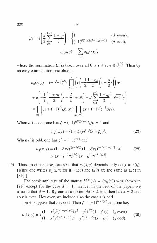
228 6

βk = e

d

2

k−1∑

l=1

1 − ηl

2

=

1 (d even),

(−1)#l|1≤l≤k−1,ηl=−1 (d odd),

uη(x, y) =∑

i,ǫ

uǫη(s)yi,

where the summation Σǫ is taken over all 0 ≤ i ≤ r, ǫ ∈ E(r)

i. Then by

an easy computation one obtains

uη(x, y) = (−√−1)dr j

r∏

k=1

(e

(−1

2

1 − ηk

2

(s − d

2r

))+

+ e

−1

2

1 + ηk

2

(s − d

2r + dk

)− d

k−1∑

l=1

1 − ηl

2

√−1dy

=

∏

ηk=1

(1 + (−1)dkζβk xy)∏

ηk=−1

(x + (−1)dζ−1βky).

When d is even, one has ζ = (−1)(d/2)(r+1), βk = 1 and

uη(x, y) = (1 + ζxy)r− j(x + ζy) j. (28)

When d is odd, one has ζ2= (−1)r+1 and

uη(x, y) = (1 + ζxy)[(r− j)/2](1 − ζxy)r− j−[(r− j)/1] × (29)

× (x + ζ−1y)[ j/2](x − ζ−1y) j−[ j/2] .

Thus, in either case, one sees that uη(x, y) depends only on j = n(η).191

Hence one writes u j(x, y) for it. [(28) and (29) are the same as (25) in

[SF].]

The semisimplicity of the matrix U(r)(x) = (ui j(x)) was shown in

[SF] except for the case d = 1. Hence, in the rest of the paper, we

assume that d = 1. By our assumption dδ ≥ 2, one then has δ = 2 and

so r is even. However, we include also the case r is odd.

First, suppose that r is odd. Then ζ = (−1)(r+1)/2 and one has

u j(x, y) =

(1 − x2y2)(r− j−1)/2(x2 − y2) j/2(1 − ζxy) ( j even),

(1 − x2y2)(r− j)/2(x2 − y2)( j−1)/2(x − ζy) ( j odd).(30)

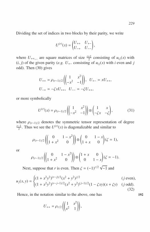
229

Dividing the set of indices in two blocks by their parity, we write

U(r)(x) =

(U++ U+−U−+ U−−

),

where U++,... are square matrices of size r+12

consisting of ui j(x) with

(i, j) of the given parity (e.g. U+− consisting of ui j(x) with i even and j

odd). Then (30) gives

U++ = ρ(r−1)/2

((1 x2

−x2 −1

)), U+− = xU++,

U−+ = −ζxU++, U−− = −ζU++,

or more symbolically

U(r)(x) = ρ(r−1)/2

((1 x2

−x2 −1

))⊗

(1 x

−ζx −ζ

), (31)

where ρ(r−1)/2 denotes the symmetric tensor representation of degreer−1

2. Thus we see the U(r)(x) is diagonalizable and similar to

ρ(r−1)/2

((0 1 − x2

1 + x2 0

))⊗

(0 1 − x

1 + x 0

)(ζ = 1),

or

ρ(r−1)/2

((0 1 − x2

1 + x2 0

))⊗

(1 + x 0

0 1 − x

)(ζ = −1).

Next, suppose that r is even. Then ζ = (−1)r/2√−1 and

u j(x, y) =

(1 + x2y2)(r− j)/2(x2

+ y2) j/2 ( j even),

(1 + x2y2)(r− j−1)/2(x2+ y2)( j−1)/2(1 − ζxy)(x + ζy) ( j odd).

(32)

Hence, in the notation similar to the above, one has 192

U++ = ρr/2

((1 x2

x2 1

)),

230 REFERENCES

U+− = x(δi j + δi, j+1)ρr/2−1

((1 x2

x2 1

)),

U−+ = 0,

U−− = ζ(1 − x2)ρr/2−1

((1 x2

x2 1

)).

Thus U(r)(x) is again diagonalizable and similar to

ρr/2

((1 + x2 0

0 1 − x2

))⊕ ζ(1 − x2)ρr/2−1

((1 + x2 0

0 1 − x2

)).

These results imply that one can simplify the functional equations,

introducing certain L-functions, and obtain some information about the

special values of the zeta functions, as was done in [SO] in the case d is

even.

References

[A] T. Arakawa : The dimension of the space of cusp forms on the

Siegel upper half plane of degree two related to a quaternion uni-

tary group, J. Math. Soc. Japan 33 (1981), 125-145.

[M] M. Muro : Microlocal analysis and calculations on some relatively

invariant hyperfunctions related to zeta functions associated with

the vector spaces of quadratic forms, Publ. RIMS Kyoto Univ. 22

(1986), 395-463.

[O] S. Ogata : Special values of zeta functions associated to cusp sin-

gularities, Tohoku Math. J. 37 (1985), 367-384.

[S1] I. Satake : Algebraic Structures of Symmetric Domains, Iwanami-193

Shoten and Princeton Univ. Press, 1980.

[S2] I. Satake : On numerical invariants of arithmetic varieties on O-

rank one, Automophic Forms of Several Variables (Taniguchi Sym-

posium, Katata, 1983), Progress in Math. 46, Birkhauser, 1984,

353-369.

REFERENCES 231

[S3] I. Satake : A formula in simple Jodan algebras, Tohoku Math. J.

36 (1984), 611-622.

[S4] T. Shintani : On zeta-functions associated with the vector space of

quadratic forms, J. Fac. Sci. Univ. Tokyo 22 (1975), 25-65.

[S5] C. L. Siegel : Uber die Zetafunktionen indefiniter quadratischer

Formen, Math. Z. 43 (1938), 393-417.

[Si] I. Satake and J. Faraut : The functional equation of zeta distribu-

tions associated with formally real Jordan algebras, Tohoku Math.

J. 36 (1984), 469-482.

[SF] I. Satake and S. Ogata : Zeta functions associated to cones and

their special values, to appear in Adv. St. in P. Math. 15.

[SO] I. Satake and S. Ogata : Zeta functions associated to cones and

their special values, to appear in Adv. St. in P. Math. 15.

[SS] M. Sato and T. Shintani : On zeta functions associated with pre-

homogeneous vector spaces, Ann. of Math. 100 (1974), 131-170.

[V] E. B. Vinberg : The theory of convex homogeneous cones, Trudy

Moskov. Mat. obsc. 12 (1963), 303-358; = Trans. Moscow Math.

Soc. 1963, 340-403.

[W] A. Weil : Sur la formule de Siegel dans la theorie des groupes

classiques, Acta Math. 113 (1965), 1-87.

Mathematical Institute

Tohoku University

Sendai 980, Japan

THE NUMBER OF RATIONAL

APPROXIMATIONS TO ALGEBRAIC

NUMBERS AND THE NUMBER OF

SOLUTIONS OF NORM FORM

EQUATIONS

By Wolfgang M. Schmidt

Recently, after i had lectured on Norm Form equations [11], Schinzel195

said : “But now can it be, how can it be in number theory, that one could

possibly prove the finiteness of a set of natural numbers, but obtain no

estimate of its cardinality ?” The next day, he himself provided the fol-

lowing answer : Suppose we can prove for a set S of natural numbers

that for any x, x′ in S we have x′ ≤ 2x. Then S is finite, but unless we

can find a particular x ∈ S , we cannot estimate the cardinality of S , and

even less can be provide a bound for the size of elements in S .

More generally, for C > 1, call a set S of positive integers a C-set, if

x′ ≤ Cx for any x, x′ ∈ S . What we said above applies more generally

to any C-set. On the other hand, we define a λ-set where λ > 1 to be

a set S with the following Gap Principle : When x, x′ are in S with

x′ > x, then x′ ≥ λx. A (C, λ)-set is both a C-set and a λ-set. Let

x0 < x1 < . . . < xv be elements of a (C, λ)-set S . Then xv ≤ Cx0 and

xi ≥ λxi−1(i = 1, . . . , v), so that xv ≥ λvx0. Therefore λv ≤ C, and

v ≤ (log C)/(log λ), so that S has cardinality

|S | ≤ 1 + (log C)/(log λ).

In this argument, we did not need to assume that S consists of integers.

232

The Number of Rational Approximations to Algebraic Numbers and the

Number of Solutions of Norm Form Equations 233

A situation very much like this occurs in the Thue-Siegel-Roth The-

orem. Let me begin with Thue’s Theorem. It asserts that when α is

algebraic of degree r ≥ 3, and if µ > (r/2) + 1, then there are only

finitely many rationals x/y with |α − (x/y)| < |y|−µ. Let Y be the set

of positive y such that there is a reduced fraction x/y which satisfies

this inequality; then Y is finite according to Thue. It is well known that

Thue’s Theorem (and subsequent theorems of Siegel, Roth, Schmidt)

are “ineffective” in the sense that they do not provide an upper bound

for the (size of) elements of Y . An analysis of Thue’s proof shows that

it yields an explicit constant B = B(α, µ), such that if S 1 is the set of

y ∈ Y with y < B(α, µ), the so-called “small solutions”, and if S 2 is the

set of y ∈ Y with y ≥ B(α, µ), the so-called “large solutions”, then the

following holds. First, it is trivial that the cardinality of S 1 does not ex-

ceed the explicit bound B(α, µ). Second, there is an explicit C = C(α, µ)

such that S 2 is an exponential C-set in the sense that

y′ ≤ yC

for any y, y′ in S 2. This shows that S 2 (and hence Y) is finite, but 196

gives no information on the cardinality. However, it turns out that there

is also an exponential Gap Principle. Suppose y′ > y lie in S 2 and

|α − (x/y)| < y−µ, |α − (x′/y′)| < y′−µ. Since Y was defined in terms of

reduced fractions, we have x/y , x′/y′ and

1

yy′≤

∣

∣

∣

∣

∣

x

y−

x′

y′

∣

∣

∣

∣

∣

≤∣

∣

∣

∣

∣

α −x

y

∣

∣

∣

∣

∣

+

∣

∣

∣

∣

∣

α −x′

y′

∣

∣

∣

∣

∣

< y−µ + y′−µ < 2y−µ,

so that y′ > 12yµ−1. Now if 1 < λ < µ − 1, say if λ = µ/2 and if

y ≥ B(α, µ) where B(α, µ) was chosen large enough, then we have

y′ > yλ,

i.e., an exponential Gap Principle. Thus S 2 is an exponential (C, λ)-set,

and its cardinality may be explicitly bounded by 1+ (log C)/(log λ). But

note that even though we can estimate the cardinality of a (C, λ)-set,

we cannot estimate the size of its elements, and hence Thue’s Theorem

remains ineffective.

234 Wolfgang M. Schmidt

The situation is similar for Siegel’s Theorem, where the condition

µ > (r/2) + 1 is relaxed to µ > 2√

r, and for the Dyson-Gelfond Theo-

rem, with the condition µ >√

2r.

Roth finally relaxed the condition to µ > 2. His Theorem says that

for α as above and δ > 0, there are only finitely many rationals x/y with

|α − (x/y)| < |y|−2−δ. Again we can form the set Y of denominators and

distinguish small solutions y < B(α, δ) and large solutions y ≥ B(α, δ).

This time we cannot assert that the large solutions form an exponential

C-set. But there are explicit C = C(α, δ) and m = m(α, δ) where m is

an integer, such that the large solutions are the union of m exponential

C-sets, hence (C, λ)-sets. This again gives a bound for the cardinality.

Explicit bounds for the number of solutions of |α − (x/y)| < y−2−δ

with y > 0 were given by Davenport and Roth [3]. More recently,

Bombieri and Van der Poorten [2] came up with better bounds by using

a new theorem of Esnault and Viehweg [4] in place of “Roth’s Lemma”.

They considered the slightly stronger inequality.

∣

∣

∣

∣

∣

α − x

y

∣

∣

∣

∣

∣

<1

64y2+δ

and showed that the number of solutions x/y in reduced form with y > 0

is

≤ log log 4H

log(1 + δ)+ 3000

(log r)2 log(50δ−2 log r)

δ5, (1)

provided that 0 < δ < δ0 with some absolute δ0. Here H = H(α) is the197

height of α (related to the naive height, which is the maximum modulus

of the coefficients of the minimal defining polynomial of α over Z).

The first summand in (1) comes essentially from the small solutions,

the second summand from the large solutions. Although initially the

small solutions appeared to be more tractable, it turns out that they are

responsible for the dependency of H in (1). In fact, the first summand

in (1) is best possible (See, e.g. [8].)

Now let us turn to simultaneous approximation. Some years ago,

I proved the following [9] : Suppose α1, . . . , αn are algebraic, with 1,

α1, . . . , αn linearly independent over O. Then there are only finitely

The Number of Rational Approximations to Algebraic Numbers and the

Number of Solutions of Norm Form Equations 235

many rational points (x1/y, . . . , xn/y) with y > 0 and

|αi − (xi/y)| < y−1−(1/n)−δ(i = 1, . . . , n) (2)

for given δ > 0. Here, when n > 1, we cannot at present estimate the

number of solutions.

Following the method in [11], we can try to find explicit B, C, m

depending only on α1, . . . , αn, δ, such that the numbers y > B occurring

in solutions of (2) (the “large solutions”) constitute not more than m

exponential C-sets. The real difficulty is with the Gap Principle.

Write α = (α1, . . . , αn), x = (x1/y, . . . , xn/y), and write (2) as

abc < y−1−(1/n)−δ, (3)

where denotes the maximum norm. Now let x0, . . . , xn be solutions

of (3) with y0 ≤ y1 ≤ . . . ≤ yn where yi = y(xi)(i = 0, . . . , n). Writing

xi = (xi1/yi, . . . , xin/yi), and assuming the determinant is not zero, we

have

1

y0y1 . . . yn

≤

∣

∣

∣

∣

∣

∣

∣

∣

∣

∣

∣

∣

∣

∣

∣

∣

∣

∣

1x01

y0. . .

x0n

y0

. . .

1xn1

yn. . .

xnn

yn

∣

∣

∣

∣

∣

∣

∣

∣

∣

∣

∣

∣

∣

∣

∣

∣

∣

∣

=

∣

∣

∣

∣

∣

∣

∣

∣

∣

∣

∣

∣

∣

∣

∣

∣

∣

∣

1x01

y0− α1 . . .

x0n

y0− αn

. . .

1xn1

yn− α1 . . .

xnn

yn− αn

∣

∣

∣

∣

∣

∣

∣

∣

∣

∣

∣

∣

∣

∣

∣

∣

∣

∣

≤ (n + 1)!(y0y1 . . . yn−1)−1−(1/n)−δ.

Therefore

yn >1

(n + 1)!(y0y1 . . . yn−1)(1/n)+δ ≥ 1

(n + 1)!y1+nδ

0

With λ = 1+(nδ/2) and y0 ≥ B large, this leads to yn > yλ0. Although this 198

would give a Gap Principle involving only every nth term in a sequence

x0, x1, . . . of approximations, it would be very useful in estimating the

number of such approximations.

Where is the catch ? The catch lies in the assumption that the above

determinant is not zero. The determinant will be zero precisely when

x0, x1, . . . , xn (with are in Rn) lie in an (n − 1)-dimensional linear sub-

manifold of Rn. Henceforth we shall call such a submanifold a hyper-

plane. E.g., when n = 2, the determinant will be zero when x0, x1, x2 lie

on a line.

236 Wolfgang M. Schmidt

So we cannot really estimate the number of solutions x of (3). What

we can do is the following (see [12]). We can give an explicit t = t(α, δ),

such that the solutions x of (3) lie in a collection of t hyperplanes.

The following argument shows why it is unlikely that we will soon

be able to estimate the number of solution x of (3) when n > 1. Given

Q > 1, the inequalities

|u| ≤ Q, |αiu − vi| ≤ Q−1/(n−1) (i = 1, . . . , n − 1)

define a parallelepiped Π of volume 2n in the space of vectors u =

(v, u1, . . . un−1). By Minkowski, there is a nonzero integer point u in

Π. In fact, for given ǫ > 0 and for large Q, the nth minimum µn = µn(Q)

of Π has µn < Qǫ (See [9]. But we don’t know how large Q has to

be). For such Q there are n independent integer points u1, . . . , un in the

blown up parallelepiped QǫΠ. The linear combinations c1u1+ · · ·+cnun

with |c1| + · · · + |cn| ≤ Qǫ lie in Q2ǫΠ. Thus for large Q, there are

≥ c(n)Qnǫ > Qǫ nonproportional integer points in Q2ǫΠ.

Suppose now that

0 < δ <1

n(n − 1)

and let ǫ have δ + 7ǫ < 1/(n(n + 1)). Suppose we have a rational hy-

perplane H which comes very close to α = (α1, . . . , αn). Say H is given

by

a0 + a1X1 + · · · + · · · + anXn = 0,

with coprime integers a0, a1, . . . , an. Suppose |an| = max(|a1 |, . . . , |an|) =a, say and H is so close to α that

|a0 + a1α1 + · · · + anαn| < a−2/ǫ . (4)

Set Q = a1/ǫ , and let u be in Q2ǫΠ(Q), so that

|u| ≤ Q1+2ǫ , |αiu − vi| ≤ Q−(1/(n−1))+2ǫ (i = 1, . . . , n − 1). (5)

Then with y = anu, xi = anvi(i = 1, . . . , n − 1) we have199

|αiy − xi| ≤ aQ−(1/n−1)+2ǫ= Q−(1/(n−1))+3ǫ (i = 1, . . . , n − 1).

The Number of Rational Approximations to Algebraic Numbers and the

Number of Solutions of Norm Form Equations 237

On the other hand, if we set xn = −(a0u+a1v1+ · · ·+an−1vn−1), then

(4) yields

|αny − xn| < naQ−(1/(n−1))+2ǫ+ |u|a−2/ǫ ≤ nQ−(1/(n−1))+3ǫ

+ Q1+2ǫQ−2

< Q−(1/(n−1))+4ǫ

if a, and hence Q, is large. When u , 0, then u , 0 by (5), so let us say

that u > 0. Then y = au ≤ Q1+3ǫ ; and since

(

1

n − 1− 4ǫ

)

/

(1 + 3ǫ) ≥ 1

n − 1− 7ǫ >

1

n+ δ,

we have∣

∣

∣

∣

∣

αi −xi

y

∣

∣

∣

∣

∣

< y−1−(1/n)−δ(i = 1, . . . , n).

This holds for u , 0 in Q2ǫΠ(Q). By what we said above, there will in

general be ≥ Qǫ non-proportional such u, and hence there will be ≥ Qǫ

solutions to (2) or (3).

This will happen if there is a single hyperplane H with (4) and with

large a. As is well known, the linear form inequality (4) is dual to simul-

taneous approximations. Thus in order to bound the number of solutions

of (2), we would have to give a bound for the size a of solutions of the

dual inequality (4). Thus we would have to have an “effective” result

on the linear forms inequality (4). But such an effective result is un-

known even in the case n = 1, since the Thue-Siegel-Roth Theorem is

ineffetive.

Now let us turn to Thue equations and Norm Form equations. A

Thue equation is an equation

F(x, y) = m, (6)

where F is a binary form of degree r ≥ 3 with rational integer coef-

ficients which is irreducible over the rationals. Over C it factors as

F = α(x − α1y) . . . (x − αry) where a ∈ Z, and α1, . . . , αr is a set

of conjugate algebraic numbers. A Norm Form equation is an equation

F(x1, . . . , xn) = m (7)

238 Wolfgang M. Schmidt

where F is a norm form, i.e.

F = a

r∏

i=1

(α(i)

1x1 + · · · + α(i)

n xn),

where α1, . . . , αn lie in an algebraic number field K of degree r, and200

where α 7→ α(1), . . . , α 7→ α(r) are the embeddings of K into C.

Using his result on approximation to algebraic numbers (applied

to α1, . . . , αr), Thus showed that (6) has only finitely many solutions.

Bounds involving m, r and the size of the coefficients of F were given

by Lewis and Mahler [6]. Siegel [14] had conjectured that there were

bounds depending only on m and r. The first such bounds were derived

by Evertse [5]. Later, Bombieri and Schmidt [1] established the bound

cr1+ω

for the number of coprime solutions x, y, where c is an absolute constant

and ω = ω(m) the number of distinct prime factors of m. Notice the

contrast with diophantine approximation, where the dependency of (1)

on the height H cannot be eliminated! Siegel also had conjectured that

there should be a bound which depends only on the number of nonzero

coefficients. It turns out that there is no bound independent of m. How-

ever, Mueller and Schmidt [7] proved Siegel’s conjecture in the modified

form that there is a bound which depends only on m and the number of

nonzero coefficients of F (but which is independent of the degree r).

Some years age ([10]), I proved that when F is “non-degenerate”,

then the equation (7) has only finitely many solutions. I now can give

an explicit bound for the number of solutions which depends only on

n, r, m, but which is independent of the coefficients of F. In fact, the

proof by induction on the number n of variables would break down if

at some stage we had dependency on the coefficients. It will be conve-

nient to formulate the result in terms of primitive solutions with g.c.d.

(x1, . . . , xn) = 1. I can prove (see [13]) that the number of primitive

solutions of a non-degenerate Norm Form equation with coefficients in

Z is

≤ C1C2

REFERENCES 239

where

C1 = min(r230n

r2

, rE) with E = (2n)n2n+4

,

C2 =

(

r

n − 1

)ω

dn−1(mr),

with dn−1(x) denoting the number of factorizations x = x1 . . . xn−1 with

positive factors.

In the proof, I write the equation as aL1 . . . Lr = m where Li =

α(i)

1x1 + · · · + α(i)

n xn(i = 1, . . . , r), and I deduce the existence of i1, . . . , insuch that Li1 , . . . , Lin are independent and 201

|Li1 (x) . . . Lin (x)| < |x|−δ | det(Li1 , . . . , Lin )| (8)

with suitable δ > 0, where x = (x1, . . . , xn), and |x| is its norm. In-

equalities (8) are derived in various ways, depending on whether x is

“small” or “large”. Then (8) is dealt with by a semieffective version of

the Subspace Theorem [11].

It is to be hoped that these results will lead to bounds for the number

of solutions of S -unit equations, and the multiplicities of linear recursive

sequences.

References

[1] E. Bombieri and W. M. Schmidt : On Thue’s equaiton, Invent.

Math., 88 (1987), 69-81.

[2] E. Bombieri and A. J. Van der Poorten : Some quantitative results

related to Roth’s Theorem, Mac Quarie Univ. Reports 1987.

[3] H. Davenport and K. F. Roth : Rational approximation to algebraic

numbers, Mathematika 2 (1955), 160-167.

[4] H. Esnault and E. Viehweg : Dyson’s Lemma for polynomials

in several variables (and the theorem of Roth), Invent. Math., 78

(1984), 445-490.

240 REFERENCES

[5] H. Evertse : Upper bounds for the number of solutions of dio-

phantine equations, Math. Centrum Amsterdam (1983), 1-127.

[6] D. Lewis and K. Mahler : Representation of integers by binary

forms, Acta Arith., 6 (1961), 333-363.

[7] J. Mueller and W. M. Schmidt : Thue’s equation and a conjecture

of Siegel, Acta Math., 160 (1988), 207-247.

[8] J. Mueller and W. M. Schmidt : The number of good rational

approximations to algebraic numbers, Proc. A. M. S. (to appear).

[9] W. M. Schmidt : Simultaneous approximation to algebraic number202

by rationals, Acta Math., 125 (1970) 159-201.

[10] W. M. Schmidt : Norm Form equations, Ann. of Math. 96(1972)

526-551.

[11] W. M. Schmidt : The Subspace Theorem in Diophantine approxi-

mations, Compositio Math., 69 (1989), 121-173.

[12] W. M. Schmidt : The number of solutions of Norm Form equations

(expository paper), Proc. Number Theory Symposium, Budapest,

July 1987, (to appear).

[13] W. M. Schmidt : The number of solutions of Norm Form equa-

tions, Trans. A. M. S. (to appear).

[14] C. L. Siegel : Uber einige Anwendungen diophantischer Approxi-

mationen, Abh. Preuss. Akad. Wiss. Phys-Math. Kl. 1929, Nr. 1.

University of Colorado

Boulder, Colorado

LINEAR OPERATORS AND

AUTOMORPHIC FORMS

By Atle Selberg

203

1 We consider a bounded symmetric complex domain B in the sense

of Elie Cartan1 and denote the group of analytic mappings of B onto

itself by G, points in B by z and the elements of G by g : z → gz.

By a multiplier (or automorphy factor) ρg(z), we understand a function

defined on G × B which is analytic (holomorphic) in z and differentiable

in g such that

ρg1g2(z) = ρg1

(g2z)ρg2(z). (1.1)

Any such multiplier defines a kernel function kρ(z, z) which transforms

in the way

kρ(gz, gz) = ρg(z)ρg(z)kp(z, z). (1.2)

We need only to write, for some fixed z0 in B,

kρ(z, z) = |ρg(z0)|2

where g is a solution of z = gz0 and it is clear that this does not depend

on the particular g chosen, but only on the point z.

From (1.2), we get that

ds2=

∑

i, j

∂2 log kp(z, z)

∂zi∂z j

· dzidz j

is an invariant metric on B under the action of the group G. Thus, if

B is irreducible, we get that this metric can differ only by a constant

1See for instance Siegel [5], Chapter XI.

241

242 1

factor from the Bergmann metric. If B is reducible, it must be a lin-

ear combination of the Bergmann metrics of the irreducible factors of

B. For irreducible B, one easily derives that, up to a factor of the form

c f (z) f (z) where f (z) is analytic, kρ(z, z) coincides with a real power of

the Bergmann kernel function and ρg(z) is, apart from a ‘trivial’ multi-

plier of the form f (gz)/ f (z), equal to a power of the jacobian jg(z) of

the mapping g. Similarly, if B is reducible, ρg(z) is, apart from a trivial

factor f (gz)/ f (z), equal to a product of powers of the jacobians of the

mapping g with respect to the various irreducible factors of B.

We may mention that essentially the same conclusion could be drawn204

from the weaker premise that instead of (1.1), ρg(z) satisfies the relation

|ρg1g2(z)| = |ρg1

(g2z)||ρg2(z)|, (1.3)

then, apart from a factor of the form ǫg f (gz)/ f (z) where f is analytic

and |ǫg| = 1, ρg(z) is equal to a product of powers of the jacobians of the

mapping z→ gz with respect to the irreducible factors of B.

We shall study linear operators on functions defined on B, which

have the property of transforming with a multiplier on each side under

the mappings of the group G. Call the operator L = Lz and define Lgz

through the relation

LgzF(z) = [LzF(g−1z)]z→gz;

then L should transform according to the rule

Lgz = ρg(z)L2σ−1g (z), (1.4)

where ρ and σ are two multipliers.2

We ask the question : for which B and which choices of multipliers

ρ and σ do such operators exist? And when they exist, determine their

form as explicitly as possible.

It is easily seen that we may restrict ourselves to the case that B is

irreducible and then derive the results for the general case from those

obtained for the irreducible factors of B in case B is irreducible.

2From now on, we disregard trivial multipliers and consider only products of powers

of the jacobians for the irreducible factors of B. This is only an apparent restriction.

243

As is known3 there are six types of irreducible bounded symmetric

domains. If we denote a matrix with m rows and n columns by Z(m,n)

and the (n, n) unit matrix E or E(n), there are the four main types :

(I) Z = Z(m,n), E − Z′Z > 0,

(II) Z = Z(n,n), Z′ = −Z, E − Z′Z > 0.

(III) Z = Z(n,n), Z′ = Z, E − Z′Z > 0, and

(IV) Z = Z(n,1), Z′Z < 1

2(1 + |Z′Z|2) < 1.

Here Z′ denotes the transposed matrix. In addition, there are the

types V and VI — the two exceptional bounded symmetric domains of

complex dimension 16 and 27 respectively; we shall not give a definition

here.

It should also be noted that for n = 2, the domain IV is reducible 205

and that there is also some overlapping between the four types for low

dimension; the unit circle |z| < 1 in one complex variable is, for instance,

a special case of all the four types.

2 The question of linear operators that transform according to the

rule (1.4) can be split in two :

(a) Operators that conserve the multiplier, i.e. when (1.4) holds, but

with ρg(z) ≡ σg(z).

We shall refer to such operators as invariant (though, strictly speak-

ing, they are so only if ρg(z) ≡ 1 identically).

It is well-known that invariant operators exist for all the bounded

symmetric domains B and for all multipliers ρg(z); for given ρ the dif-

ferential operators form a finitely generated ring, where the number of

independent generators equals the rank of the group G (or of the sym-

metric space). In this ring, all elements, except the constant, contain

3See Siegel [5], Chapter XI for instance.

244 2

differentiations both with respect to z and z. The form of integral opera-

tors is easily given explicitly for B irreducible; if ρg(z) = ( jg(z))−r where

jg(z) denotes the jacobian of the mapping g, then

L f =

∫

B

x(z, ζ)

(k(z, η)

k(ζ, ζ)

)r

f (ζ)dωζ (2.1)

where dωζ is the invariant volume element, k(z, ζ) is the Bergmann ker-

nel function and x(z, ζ) is a “point pair invariant” satisfying x(gz, gζ) =

x(z, ζ) for all z and ζ in B and g in G.

In particular, for analytic functions f (z), we have the reproducing

operator

f (z) = cr

∫

B

k(z, ζ)

k(ζ, ζ)

r

f (ζ)dωζ (2.2)

where cr is a certain polynomial in r. (2.2) is valid for a certain hilbert-

space of analytic functions if r > r0, the largest zero of the polynomial

cr.4

(b) Operators that change the multiplier, i.e. which transform in the

way (1.4) but with ρg(z) . σg(z).

The question (b) is more complex than (a), but it is not difficult to

establish that linear operators that change the multiplier do not exist for

all the irreducible domains, but only for a certain subclass.

To see this, we may look at the compact subgroup of G which leaves

some point z0 in B fixed, the so-called stability group or isotropy group206

of z0. It is simplest to choose the point O where all the coordinates

are zero and the compact subgroup K0 which keeps O fixed. For all

the six types of bounded symmetric domains, the way they are usually

defined, the elements of K0 are linear transformations, and K0 is essen-

tially (sometimes, a slight change of variables being necessary as in type

III where we would put a factor 1/√

2 in the elements of the symmetric

matrix which are off the main diagonal) a subgroup of the unitary group

4See Selberg [4]

245

U(N) where N is the complex dimension of B and jk(z) = jk(0), where

k ∈ K0, is a one-dimensional representation of K0.

It is clear that if there exists a linear operator satisfying (1.4), then,

in particular, (1.4) must hold for g restricted to K0 and we consider the

functional L that Lz represents at z = 0.

On the other hand, it is not hard to show that if we have a linear

functional L which has the required property (1.4) for g in K0, then it

can be extended to a linear operator Lz by means of the relation (1.4)

with z = gO, but the general form of this operator seems awkward to

obtain in this way, particularly if it is a differential operator.

It is easily seen that an integral operator

Lz f =

∫

B

h(z, ζ) f (ζ)dωζ

where h(z, ζ) is a short form for h(z, z, ζ, ζ), must in order to satisfy (1.4),

have a kernel h(z, ζ) which satisfies

h(gz, gζ) = ρg(z)σ−1g (ζ)h(z, ζ) (2.3)

and, in particular, for g = k ∈ K0, if we put ζ = 0, we get

h(kz, 0) = ρk(z)σ−1k (0)h(z, 0)

or since ρk(z) = ρk(0),

h(kz, 0) = ρk(0)σ−1k (0)h(z, 0). (2.4)

Since we may assume that h(z, ζ) is analytic in z and z5, it is clear that

the expansion of h(z, 0) in terms of powers of z and z for z near 0, must

start with a homogeneous polynomial ρ(z, z) which also transforms by

the factor ρk(0)σ−1k

(0) when we replace z by kz.

Similarly, if Dz is a differential operator which obeys the transfor- 207

5If our original h(z, ζ) is not so, we may form the convolution of Lz with a suitable

operator of the form (2.1) on the left which preserves the multiplier ρg(z).

246 2

mation rule (1.4), at z = 0 it takes the form of a polynomial in∂

∂zand

∂

∂z:

D0 = P

(∂

∂z,∂

∂z

).

When z and so dz undergoes a unitary transformation from K0,∂

∂zun-

dergoes the contragredient transformation; so we are again led to a poly-

nomial (which we may assume to be homogeneous, otherwise taking the

homogeneous part of lowest degree that is not identically zero) which

transforms in the way (2.4) when the variables undergo the contragre-

dient transformation to k (Actually, if we interchange∂

∂zand

∂

∂z, the

vector

(∂

∂z,∂

∂z

)undergoes the same transformation as (z, z)).

It is now easy to see for the various types of B whether such poly-

nomials exist when ρg(z) . σg(z).

We find that for type I, they exist only if m = n and are then of the

form

|z|rP(z, z) or |z|rP(z, z)

where |z| is the determinant of z, r some positive integer and P(z, z) some

homogeneous polynomial which is invariant under K0.

For type II, they exist only if n is even and are then of the form

Prf (z)P(z, z or Pr

f (z)P(z, z)

where P f (z) is the polynomial called the Pfaffian of z (actually |z|1/2,

since the determinant is a square in this case), r again is a positive

integer and P, a homogeneous polynomial which is invariant under K0.

For type III, they exist for all n and are of the form

|z|rP(z, z) or |z|rP(z, z)

where r is a positive integer and P(z, z) homogeneous and invariant un-

der K0.

247

For type IV, they again exist and are of the form

(z′ z)rP(z, z) or (z′ z)rP(z, z)

with r a positive integer and P(z, z) again homogeneous and invariant

under K0.

For the types V and VI which (for good reason!) we have not exhib- 208

ited explicitly, we find they do not exist for type V but, for type VI, they

exist and are given by the form

p3(z)rP(z, z) or p3(z)rP(z, z)

where r and P are as before and p3 is a certain cubic polynomial in 27

variables.

3 In order to derive more explicitly the form of the linear operators

that transform according to (1.4) in the cases where we have seen they

can exist, we note that the cases we have listed in the previous section

are precisely the cases when the bounded domain B, by a suitable an-

alytic mapping, becomes a so-called “positive half-space”6 , and when

the group G by this mapping, becomes a real group (by which we mean

that in this new unbounded version of our domain, we have gz = gz).

By a positive half-space, we understand a domain of z = x + iy,

where the column vector x is unrestricted, while the vector y is required

to lie in a homogeneous positivity-domain Y in the sense of Koecher7.

As before, we shall use N to denote the complex dimension.

We recall some of the properties of a homogeneous positivity do-

main Y . It is a cone such that, for any two vectors y(1) and y(2) in Y , we

have always

y(1)y(2) > 08 (3.1)

6M. Koecher [2] writes “half-space”; I prefer “positive half-space” since it indicates

the connection with a positivity-domain.7M. Koecher [1]8Koecher’s definition is more general; he has (3.1) in the form y(1)S y(2) > 0, where

S is a nonsingular symmetric real matrix, but (3.1) covers the cases we consider.

248 3

and so that if, for some vector y(1), (3.1) holds for all y(2) in Y , then y(1)

also lies in Y .

There also exists a group GY of real matrices A such that y → Ay

maps Y onto itself; this group is transitive on Y . In particular, for any

scalar λ > 0, we have λy ∈ Y for y ∈ Y , so that Y is a cone. It is seen

from (3.1) that if A is in GY , then y→ A′−1y also maps Y onto itself; so,

we may, without restriction, assume that with A, always A′−1 also lies

in GY .

There exists a homogeneous polynomial Q(y), which we choose to

be of minimal degree q > 0 such that Q(y) is positive in Y and

Q(Ay) = |A|q/N Q(y)9 (3.2)

If we define for i = 1, . . . ,N,9209

y∗i =∂ log Q(y)

∂yi

, (3.3)

then y→ y∗ is an involution which carries Y into itself. We have9

Q(y∗)Q(y) = constant, (3.4)

and, by a suitable choice of Q (which by (3.2) is only determined up to

a constant factor) we get

Q(y∗)Q(y) = 1 (3.4′)

Also, (3.2) gives y∗′y = q and (A y)∗ = A′−1y∗.

On Y , we have an invariant volume element

dVy = (Q(y)−N/qdy (3.5)

where we have written dy for the euclidean volume element. We also

have an invariant metric

ds2= −

∑

1≤i, j≤N

∂2

∂yi∂y j

log Q(y)dyidy j. (3.6)

9Our Q(y) = (N(y))q/N , where N(.) is Koecher’s “Norm-function”.

249

The involution y → y∗ (which is actually a symmetry) has a fixed point

e and we have Q(e) = 1.

Now consider the positive half-space of z = x + iy where x is unre-

stricted and y is in Y and the group generated by translations of the form

z→ z+ a where a is a real vector, z→ Az for A in GY and z→ z∗ where

z∗i = −∂

∂zi

log Q(z), for i = 1, . . . ,N.

We call this group G.

If we write

Dz = Q

(∂

∂z

), (3.7)

we shall show that for g in G,

Drgz = ( jg(z)−(1/2)(rq/N+1)Dr

z( jg(z))−(1/2)(rq/N−1) (3.8)

where r is any positive integer. If gz = z+a, (3.8) is obvious and also for

gz = Az with A in GY so we really need to prove (3.8) only for gz = z∗.

To do this, we first look at the Y space. Actually Y is a symmetric

space; for any two points y(1) and y(2) in Y , there exists an A in GY such

that Ay(1)= y(2)∗, Ay(2)

= y(1)∗. Thus GY and the ∗ operation satisfy the 210

conditions for G and µ in Selberg [3].10

Also, we see that if r is a positive integer, then

Ly = Qr(y)Qr

(∂

∂y

)(3.9)

is an operator invariant under the group GY .

It follows from a general result11 that under the ∗ operation the op-

erator L given by (3.9) goes into the formal adjoint L∗ with respect to

the invariant measure dVy or otherwise expressed

Lv∗ = L∗y

10See Selberg [10], p. 51.11See Selberg [3], top of p. 53. In the context given there, the proof is obvious.

250 3

Thus for two suitable functions f and g, we have

∫

Y

f (y)Lyg(y)(Q(y))−N/qdy =

∫

Y

g(y)L∗y f (y)(Q(y))−N/qdy.

Inserting the expression for L, we see that it is easy to find the formal

adjoint L∗, since the formal adjoint of Qr

(∂

∂y

)with respect to the eu-

clidean measure is Qr

(−∂

∂y

)= (−1)rqQr

(∂

∂y

). We get

∫

Y

f (y)Lg(y)(Q(y))−N/qdy =

∫

Y

f (y)(Q(y)r−N/qQr

(∂

∂y

)g(y)dy

=

∫

Y

g(y)Qr

(− ∂∂y

)(Q(y))r−N/q f (y)dy

=

∫

Y

g(y)

(Q(y)N/qQr

(−∂

∂y

)Q(y)r−N/q f (y)

)×

× dy

(Q(y))N/q.

Thus

L∗ = QN/q(y)Qr

(−∂

∂y

)Qr−N/q(y).

Also211

L∗ = Qr(y∗)Qr

(∂

∂y∗

)

= Q−r(y)Qr

(∂

∂y∗

).

Comparing these two expressions for L∗, we get

Qr

(∂

∂y∗

)= Qr+N.q(y)Qr

(−∂

∂y

)Qr−N/q(y) (3.10)

251

= (−1)rqQr+N/q(y)Qr

(∂

∂y

)Qr−N/q(y).

But, from (3.10), it follows immediately that

Qr

(∂

∂z∗

)= Qr+N/q(z)Qr

(∂

∂z

)Qr−N/q(z). (3.11)

It remains to determine the jacobian of the mapping z→ z∗ or j∗(z). We

have∂z∗

i

∂z j

= −∂2

∂zi∂z j

log Q(z)

so that

j∗(z) =

∣∣∣∣∣∣−∂2

∂zi ∂z j

log Q(z)

∣∣∣∣∣∣ .

If, as before, dy denotes the euclidean volume element, we have, for

the invariant volume element in Y ,

(Q(y∗))−N/qdy∗ = (Q(y))−N/qdy

or using (3.4′),

dy∗ = (Q(y))−2N/qdy.

Since the symmetry y → y∗ preserves orientation or not according as N

is even or odd, we get

∣∣∣∣∣∣∂y∗

i

∂y j

∣∣∣∣∣∣ = (−1)N(Q(y))−2N/q,

or

∣∣∣∣∣∣∂2 log Q(y)

∂yi ∂y j

∣∣∣∣∣∣ = (−1)N(Q(y))−2N/q.

It is therefore obvious that 212

j∗(z) =

∣∣∣∣∣∣−∂2 log Q(z)

∂zi ∂z j

∣∣∣∣∣∣ = (Q(z))−2N/q.

Combining this with (3.11), we get that (3.8) holds also for gz = z∗; thus

(3.8) holds for all g in G.

252 3

It is however clear that (3.8), which is really an algebraic identity,

holds in a much larger group than G. Let us define GY as the group

of complex matrices whose entries satisfy the algebraic relations which

define GY and consider the group G generated by translations z→ z + a

where a may now be a complex vector, z → Az for A in GY and z → z∗.Clearly (3.8) as an algebraic identity holds for any transformation g in

G.

The transformations of G do not, in general, map the positive half-

space onto itself. G is actually large enough to map the positive half-

space back into a bounded symmetric domain-in most cases, the original

one (this being, for instance, true for the first three types listed at the

end of §2) — or one may have to add a final unitary transformation

which does not lie in K0 (this being the case for type IV where the

transformation z1 → z1, z j → iz j for 1 < j ≤ n would be needed at

the end; for type IV, the positivity domain can be defined as y1 > 0,

y21− y2

2− · · · − y2

n > 0 and we have Q(y) = 12(y2

1− y2

2− · · · − y2

n); so

the last transformation is needed to transform z21− z2

2− · · · − z2

n into

z′z = z21+ · · · + z2

n). At any rate, we get, in each case, the form of

the differential operator and its transformation formula for the original

bounded domain.

In the case of type I with m = n, we get, writing

∣∣∣∣∣∂

∂Z

∣∣∣∣∣ for

∣∣∣∣∣∣∂

∂zi j

∣∣∣∣∣∣, that

if

gZ = (AZ + B)(CZ + D)−1

where A, B, C, D are complex (n, n) matrices such that∣∣∣ A B

C D

∣∣∣ = 1, then

∣∣∣∣∣∂

∂gZ

∣∣∣∣∣r

= |CZ + D|r+n

∣∣∣∣∣∂

∂Z

∣∣∣∣∣r

|CZ + D|r−n. (3.12)

In the case of type II, for Z = Z(2n,2n) and Z′ = −Z, let g be the213

transformation

gZ = (AZ + B)(CZ + D)−1

where A, B, C and D are (2n, 2n) complex matrices with the property

that for M =(

A BC D

), J =

(O EE O

), we have

M′JM = J

253

and |M| = 1. Then writing P f

(∂

∂Z

)for P f

(∂

∂zi j

)where P f is the Pfaf-

fian, we have

(P f

(∂

∂gZ

))r

= |CZ+D|(r+2n−1)/2

(P f

(∂

∂Z

))r

|CZ+D|(r−2n+1)/2. (3.13)

For type III, if we define

∣∣∣∣∣∂

∂Z

∣∣∣∣∣ =∣∣∣∣∣∣1 + δi j

2

∂

∂zi j

∣∣∣∣∣∣

where δi j is the Kronecker symbol (1 on the main diagonal, 0 off it) and

gZ = (AZ + B)(CZ + D)−1 where, for M =(

A BC D

), I =

(0 −EE 0

), we have

M′IM = I and |M| = 1, then again

∣∣∣∣∣∂

∂gZ

∣∣∣∣∣r

= |CZ + D|r+(n+1)/2

∣∣∣∣∣∂

∂Z

∣∣∣∣∣r

|CZ + D|r−(n+1)/2. (3.14)

In the case of type IV, we will confine ourselves to stating the form

for the original bounded domain without defining the more general group

G or giving the explicit forms of g or the jacobian jg(z).

If we define Dz =

n∑i=1

∂2

∂z2i

, then

Drgz = ( jg(z))−(r/n+1/2)Dr

z( jg(z))−(r/n−1/2) . (3.15)

For the type VI, we do not give explicit formulas.

Since these differential operators only contain differentiations with

respect to z and not z, we see that if, for real α, we put in a factor

(k(z, z))−α on the left side and a factor (k(z, z))α on the right (k being

again the Bergmann kernel function), we again get an operator which

satisfies (1.4) but the two multipliers ρg and σg have each been multi-

plied by ( jg(z))α.

Besides the operators D so constructed, we may, of course, also 214

consider their complex conjugates D. These do not satisfy (1.4), since

254 4

we required our multipliers to be analytic in z. We note that D would

transform in the way

Dgz = ( jg(z))−α

Dz( jg(z))β,

where α and β depend on D. If we now define

Dz = (k(z, z))−αDz(k(z, z))β,

we see that

Dgz = ( jg(z))αDz( jg(z))−β

and so this operator has the required behaviour. Here, since the differ-

entiations in Dz are with respect to z and not z, we can clearly replace

the pair (α, β) by any other pair of real numbers (α′, β′) as long as

α′ − β′ = α − β.

It can be shown that all differential operators which satisfy (1.4) can

be obtained by combining the operators D or D with suitable invariant

differential operators of the kind mentioned under (a) at the beginning

of §2.

4 To find the general form of integral operators that transform in the

required way, we may again look at the representation of the domain B

as a positive half-space where the analytic mappings gz are real, which

is to say : gz = gz. We have, of course, also that jg(z) = jg(z).

Considering the Bergmann kernel function of this half-space, we get

thus

k(gz, gζ) = k(gz, gζ)

= ( jg(z) jg(ζ))−1k(z, ζ)

= ( jg(z) jg(ζ))−1k(z, ζ).

If we now write ζ instead of ζ, this becomes

k(gz, gζ) = ( jg(z) jg(ζ))−1k(z, ζ).

255

From this, we see that if we put

ha,b(z, ζ) =(k(z, ζ))(a+b)/2(k(z, ζ))(a−b)/2

(k(ζ, ζ))(a+b)/2, (4.1)

where b > a and b − a is such that (k(z, ζ))(a−b)/2 is single-valued for z 215

and ζ in the positive half-space12 , then (4.1) transforms in the way given

by (2.3), with ρg(z) = ( jg(z))−a, σg(ζ) = ( jg(ζ))−b.

If b < a, we write

ha,b(z, ζ) =ka(z, z)

kb(ζ, z)hb,a(ζ, z). (4.1′)

The most general form of a kernel which transforms in the way given by

(2.3) is of the form

h(z, ζ) = x(z, ζ)ha,b(z, ζ) (4.2)

where x is an invariant of the point pair z and ζ while ha,b(z, ζ) is given

by (4.1) or (4.1′) according to the sign of b − a.

For the bounded domains, the form of the kernels is more compli-

cated than for the positive half-spaces.

5 For the reducible bounded symmetric domains, these same ques-

tions can be answered by using our results for the irreducible factors.

It is possible to generalize the problem we considered and ask sim-

ilar questions for, say, bilinear operators operating on two functions are

more generally, q-linear operators acting on q functions; for instance, to

be able to produce from two automorphic forms a new one which de-

pends linearly on these two, but whose multiplier is not the product of

the multipliers of these two forms. Again, one would begin by looking

at the stability group of the point O in B. Thus, for instance, it is easy to

show that such bilinear operators exist for type I of Z(m,n)= Z(2n,n),

12This is true if b − a is an integral multiple of aN

, since it is not hard to show that

apart from a constant factor k(z, ζ) is equal to (Q(z−ζ2i

))−2N/q.

256 REFERENCES

whereas for Z(n,1) there are no such q-linear operators for q < n.13

Whether such multi-linear operators are of much interest is doubtful.

I originally determined the explicit transformation formulas for the

differential operators considered in §3, in the year 1960. My first aim

was to construct operators that effected the shift in automorphy factors

in the same way as the operators yαdk

dzky−α and yk+1 dk

dzkyk−1 do in the

case of the upper half-plane.

Later, I used them to effect analytic continuation of Dirichlet se-

ries associated with the Fourier expansions of modular forms in pos-216

itive half-spaces where the Fourier expansion contains singular terms,

and also to get the analytic continuation for the Dirichlet series associ-

ated with two such modular forms in the case when singular terms are

present.

I lectured off and on, on these matters, the first time in Hamburg in

the summer of 1961, later at various conferences, at Copenhagen (1964),

Jyvaskyla (1970), Bar Ilan (1981) and other places abroad.

In the sixties, some of the applications were privately communicated

to Hans Maass, Howard Resnikoff and Audrey Terras, all of whom (with

my permission) utilised some of this material in their publications.

References

[1] M. Koecher : Positivitatsbereiche im Rn, American Jour. Math.

79(1957), 575-596.

[2] M. Koecher : Automorphic forms in half-spaces, Seminars on An-

alytic Functions, Institute for Advanced Study, Princeton, New

Jersey, Vol. 2 (1957), 105-119.

[3] A. Selberg : Harmonic analysis and discontinuous groups in

weakly symmetric Riemannian spaces with applications to Dirich-

let series, Jour. Indian Math. Soc., 20 (1956), 47-87.

13More generally, for m ≥ n, such q-linear operators exist iff q ≥ m/n.

REFERENCES 257

[4] A. Selberg : Automorphic forms and integral operators, Seminars

on Analytic Functions, Institute for Advanced Study, Princeton,

New Jersey, Vol. 2 (1957), 152-161.

[5] C. L. Siegel : Analytic Functions of Several Complex Variables,

Institute for Advanced Study Lecture Notes, Revised edition 1962.

Institute for Advanced study

Princeton N. J. 08540, U.S.A.

SOME EXPONENTIAL DIOPHANTINE

EQUATIONS (II)

By T. N. Shorey

217

1 Ramanujan [19] observed in 1913 that

12+ 7 = 23, 32

+ 7 = 24, 52+ 7 = 25

112+ 7 = 27, (181)2

+ 7 = 215.(1)

We are looking for the solutions of

x2+ 7 = 2m in integers x > 0,m > 0. (2)

Ramanujan [19] conjectured in 1913 that all the solutions of (2) are

given by (1). Nagell [17] confirmed this conjecture in 1948. Equation

(2) is known as Ramanujan-Nagell equation.

Ratet [20] observed in 1916 that

31 =25 − 1

2 − 1=

53 − 1

5 − 1. (3)

Thus 31 has all the digits equal to one with respect to the base 2 as well

as the base 5. The next year, Goormaghtigh [11] found an other integer

satisfying a similar property :

8191 =213 − 1

2 − 1=

903 − 1

90 − 1. (4)

The letter N denotes an integer greater than two and we write ω(N − 1)

for the number of distinct prime factors of N − 1. Let us consider the

following equation which gives (3) and (4) :

N =2n − 1

2 − 1=

y3 − 1

y − 1in integers n > 0, y > 2. (5)

258

259

By completing square on the right hand side of (5), we obtain

4N + 4 = (2y + 1)2+ 7 = 2n+2.

Now, we apply the above mentioned result of Nagell to derive that (5)

has no solution other than the ones given by (3) and (4).

More general than equation (5) is

N =y

n1

1− 1

y1 − 1=

yn2

2− 1

y2 − 1in integers y1 > 1, y2 > 1, n1 > 2, n2 > 2.

Thus N has all the digits equal to one with respect to the base y1 as well

as the base y2. Let S (N) denote the set of all integers y with 1 < y < N−1

such that N has all the digits equal to one with respect to the base y. 218

Further, we put

s(N) = |S (N)|.

Thus

s(31) = s(8191) = 2.

A conjecture, due to Ratat and Goormaghtigh, states that

s(N) ≤ 1, N , 31 and N , 8191. (6)

Goormaghtigh [11] checked this conjecture for N < (10)4. For y ∈S (N), we have

N =yn − 1

y − 1, n ≥ 3. (7)

We put

n = l(N; y). (8)

For an integer v > 1, we denote by P(v) the greatest prime factor of v

and ω(v) the number of distinct prime divisors of v. Further, we write

P(1) = 1 and ω(1) = 0. Then, the author [29] proved the following

result.

Theorem 1. Let

N , 31, N , 8191 and ω(N − 1) ≤ 5. (9)

260 1

There is at most one y ∈ S (N) such that l(N; y) is odd.

If N is a prime number, then we see from (7) and (8) that l(N; y) is

an odd prime and hence, we derive

Corollary 1. For a prime N satisfying (9), we have

s(N) ≤ 1.

Thus, the conjecture (6) is valid for all primes N satisfying ω(N −1) ≤ 5. By sieve methods, it is known that the number of primes N ≤ Z

with ω(N − 1) ≤ 5 is at least constant times Z(log Z)−2. The equation

yn1

1− 1

y1 − 1=

yn2

2− 1

y2 − 1in integers y1 > 1, y2 > 1, n1 > 2, n2 > 2 (10)

has been considered by several authors. The first results are due to

Makowski and Schinzel [14]. Further, Davenport, Lewis and Schinzel

[6] applied a theorem of Siegel on integer points on curves to show

that equation (10) with fixed n1 and n2 has only finitely many solu-

tions in integers y1 > 1 and y2 > 1. It follows from Baker’s effective

version [2] of Thue’s theorem [36] that equation (10) implies that max

(n1, n2) is bounded by an effectively computable number C depending

only on y1 and y2, The author [26] applied a theorem of Baker [1] on

the approximations of certain algebraic numbers by rationals proved by219

hyper-geometric method that there are at most 17 pairs (n1, n2) satisfy-

ing (10). Balasubramanian and the author [4] applied the theory of linear

forms in logarithms to show that the number C, as above, depends only

on the greatest prime factor of y1y2. See also [23] and [27]. Finally,

it follows from a theorem of Schinzel and Tijdeman [22] that equation

(10) implies that mas (n1, y2) is bounded by an effectively computable

number depending only on y1 and n2. Hence, equation (10) has only

finitely many solutions if any two out of the four variables y1, y2, n1, n2

are fixed.

A weaker conjecture than (6) states that

s(N) < C1, N = 3, 4, . . .

261

where C1 > 0 is an effectively computable absolute constant. See Lox-

ton [13] where he derived from the theory of linear forms in logarithms

that

s(N) = Oǫ((log N)(1/2)+ǫ ), ǫ > 0. (11)

The author [29] proved that

s(N) ≤

max(2ω(N − 1) − 3, 0) if ω(N − 1) ≤ 4

2ω(N − 1) − 4 if ω(N − 1) > 4(12)

in an elementary way. If ω(N − 1) is small, we observe that (12) is more

precise than (11). Finally, it is easy to observe that s(N) < ω(N − 1)

whenever N is prime.

In this paragraph, we suppose that N is a perfect power. Then, we

can combine theorem 1 with [32, theorem 5(iv)] to derive that s(N) ≤ 1

for every N exceeding certain effectively computable absolute constant

C2 and satisfying ω(N − 1) ≤ 5. In fact, it has been conjectured that

s(N) = 0 for N > C2 and we refer to [27] for an account of results

proved in this direction.

Suppose that N−1 is a perfect power, say a q-th perfect power. Then,

we subtract one on both the sides of (7) to derive that

N − 1 = yyn−1 − 1

y − 1, y ∈ S (N).

Consequently, we see that both y as well as (yn−1 − 1)/(y − 1) are q-th

perfect powers. Now, we apply [25, theorem 3] to obtain the following

result.

Theorem 2. There exists an effectively computable absolute constant C3 220

such that s(N) = 0 whenever N − 1 is a perfect power and N > C3.

In other words, the equation

zq+ 1 =

yn − 1

y − 1in integers z > 1, q > 1, y > 1, n > 2.

has only finitely many solutions. Furthermore, this assertion is effective.

262 2

2 Let us put

u0 = 1, u1 = 9, um = 3um−1 − 2um−2(m ≥ 2).

It is easy to check that

um = 2m+3 − 7(m ≥ 0).

Ramanujan-Nagell equation (2) asks for squares in this binary recursive

sequence. By Nagell, there are only five squares in this sequence. Sev-

eral authors have worked on finding perfect powers in binary recursive

sequences. For example, in the Fibonacci sequence

u0 = 0, u1 = 1, um = um−1 + um−2(m ≥ 2),

Cohn [5] and Wyler [37], independently, proved that

u0 = 0, u1 = 1, u2 = 1, u12 = 144

are the only squares and London and Finkelstein [12] showed that

u0 = 0, u1 = 1, u2 = 1, u6 = 8

are the only cubes. It has been derived from the theory of linear forms

in logarithms that there are only finitely many perfect powers in a non-

degenerate binary recursive sequence. See Petho [18] and Shorey and

Stewart [30]; the latter paper and [31] contain also applications of this

and related results to certain Diophantine equations.

Now, we turn to define a non-degenerate binary recursive sequence.

Let r, s ∈ Z with s , 0 and r2+ 4s , 0. Let u0, u1 ∈ Z and

um = rum−1 + sum−2(m ≥ 2).

Let α and β be roots of X2 − rX − s. Observe that αβ , 0 and α , β.

Further

um = aαm+ bβm (m ≥ 0) (13)

where

a =u0β − u1

β − α, b =

u1 − u0α

β − α. (14)

263

The sequence um∞m=0is called non-degenerate if ab , 0 and α/β is not

a root of unity. Ramanujan’s τ-function satisfies the following recursive221

relation :

u0 = 0, u1 = 1, um = τ(p)um−1 − p11um−2(m ≥ 2, p prime)

and

um = τ(pm−1) (m ≥ 1).

Let αp and βp be roots of X2 − τ(p)X + p11. Then, by (13) and (14), we

have

um+1 = τ(pm) =αm+1

p − βm+1p

αp − βp

(15)

This sequence is non-degenerate whenever τ(p) , 0. Further, by Deligne,

|αp| = |βp| = p11/2.

It is well-known that Thue-Siegel-Roth-Schmidt method and Gel’-

fond-Baker theory of linear forms in logarithms are powerful tools in

studying recursive sequences. In particular, these methods can be ap-

plied to obtain some results on Ramanujan’s τ-function. For example,

an estimate of Baker [3] applied to (15) gives

|τ(pm)| ≥ p(11m/2)−C4 log(m+1) if τ(pm) , 0.

Here C4 > 0 is an effectively computable absolute constant. The author

[28] applied this estimate together with [33, Corollary 7.1] to obtain the

following result.

Theorem 3. Let p be a prime number such that τ(p) , 0. Then

τ(pm) = τ(pn) (m , n)

implies that

max(m, n, p) ≤ C5

where C5 > 0 is an effectively computable absolute constant.

We refer to [16] and [28] for an account of applications of the theory

of linear forms in logarithms to Ramanujan’s τ-function.

264 3

3 This section is a continuation of §1 of [27]. Erdos [7] and Rigge

[21], independently, proved that the product of two or more consecutive

positive integers is never a square. Erdos and Selfridge [9], by develop-

ing on an elementary method of Erdos [8], confirmed an old conjecture

by proving that the product of two or more consecutive positive integers

is never a power. In this section, we consider the corresponding problem

for consecutive members of an arithmetical progression.

First, we introduce some notation. Let b > 0, d > 0, m > 0, y > 0,

k > 2 and l ≥ 2 be integers such that P(b) ≤ k and (m, d) = 1. Let222

d1 be the maximal divisor of d such that all the prime divisors of d1 are

. 1(mod l) and we write d2 = d/d1. We consider the equation

m(m + d) . . . (m + (k − 1)d) = byl. (16)

We shall follow this notation, without reference, in this section. As

already stated, equation (16) with d = b = 1 is not possible. Also, due

to Fermat and Euler, equation (16) with b = 1, l = 2 and k = 4 is not

possible.

Erdos conjectured that equation (16) with b = 1 implies that k is

bounded by an effectively computable absolute constant. Under certain

restrictions, we wish to confirm this conjecture for equation (16). For

this, it is natural to exclude the case that

P(m(m + d) . . . (m + (k − 1)d)) ≤ k. (17)

Then, we refer to [34] to observe that (17) implies that either d = 1 or

m = 2, d = 7, k = 3. Therefore, we always suppose, without reference,

that

P(m(m + d) . . . (m + (k − 1)d)) > k if d = 1 and b > 1. (18)

By a well-known theorem of Sylvester, the assumption (18) is certainly

satisfied whenever m > k.

Marszalek [15] confirmed the conjecture of Erdos for a fixed d.

265

More precisely, he proved that equation (16) with b = 1 implies that

k ≤ exp(C6d3/2) if l = 2,

k ≤ exp(C7d7/3) if l = 3,

k ≤ C8d5/2 if l = 4,

k ≤ C9d if l ≥ 5,

(19)

where C6, C7, C8 and C9 are explicitly given absolute constants.

The author [27] proved that equation (16) with l ≥ 3 implies that k

is bounded by an effectively computable number depending only on the

greatest prime factor of d. Also, the author [27] confirmed the conjec-

ture of Erdos whenever d2 = 1 and l ≥ 3.

Suppose the equation (16) is satisfied. Then, Shorey and Tijdeman

[35]1 proved that k is bounded by an effectively computable number

depending only on l and ω(d). More precisely, they proved that

lω(d) > C10k/ log k (20)

where C10 and the subsequent letters C11, . . . ,C28 are effectively com- 223

putable absolute constants. Further, in [35], they sharpened the above-

mentioned result of the author by proving that

(d ≥)d2 > C11kl−2. (21)

We combine (20) and (21) to conclude that

d ≥ kC12(log log k)/(log log log k), k ≥ C13.

This improves considerably the estimates (19).

For ǫ > 0, Shorey and Tijdeman [35] proved that equation (16) with

k ≥ C′14= C′

14(ǫ) implies that

m ≤ d2k1+ǫ if l = 2

1We refer to [35] for more general and more precise versions of the results stated

here from [35].

266 3

and

m + (k − 1)d ≤ C15kdl/(l−2)

2if l ≥ 3. (22)

We show that the estimate (22) is quite precise for sufficiently large l.

Theorem 4. Suppose that equation (16) is satisfied. There exist effec-

tively computable absolute constants C16 > 0 and C17 > 0 such that for

k > C16, we have

m ≥ d1−C17∆l (23)

where

∆l = l−1(log l)2(log log(l + 1)). (24)

We combine (23) and (21) to derive the following result.

Corollary 2. There exists an effectively computable absolute constant

C18 > 0 such that equation (16) with l ≥ C18 implies that k is bounded

by an effectively computable number depending only on m.

We may combine Corollary 2 and (20) to conclude that equation

(16) implies that k is bounded by an effectively computable number de-

pending only on m and ω(d). The proof of theorem 4 depends on the

estimates of Baker [3] and the author [24, lemma 2] on linear forms in

logarithms.

Proof of theorem 4. We denote by C19, . . . ,C28 effectively computable

absolute positive constants. We may assume that k ≥ C19 with C19

sufficiently large. We may also suppose that l ≥ C19, otherwise (23)

follows immediately. We suppose that

m < d1−∆l (25)

and we shall arrive at a contradiction.

By (16), we have224

m + id = aixli (0 ≤ i < k) (26)

where ai and xi are positive integers satisfying

P(ai) ≤ k,

xi,∏

p≤k

p

= 1.

267

We put

S = a0, . . . , ak−1.

In view of the theorem of Erdos and Selfridge mentioned in the begin-

ning of this section, we may assume that b > 1 whenever d = 1. Then,

we derive from (18) and [34] that the left hand side of (16) is divisible

by a prime > k. Now, it follows from (16) that

m + (k − 1)d ≥ (k + 1)l

which, by (25), implies that

m + d ≥ kl−1, d ≥ kl−1/2. (27)

We denote by S 1 the set of all ai with 1 ≤ i < k such that xi = 1.

Observe, by (26), that the elements of S 1 are distinct. Now, we apply an

argument of Erdos (see [10], lemma 2.1) to derive from (27) that

|S 1| ≤ k/2 + π(k).

We denote by T the set of all i with 1 ≤ i < k such that ai < S 1 and we

write S 2 for the set of all ai ∈ S with i ∈ T . Then

|T | ≥ k/4. (28)

We put

bi = ai/i (i ∈ T )

and let S ′ be the set of all bi with i ∈ T . Let i ∈ T , j ∈ T with i > j and

bi = b j. Then, by (26),

jai(xli − xl

j) = ( j − i)m. (29)

Now, we observe that the left hand side of (29) exceeds

( j − i)(ai xli)

(l−1)/l ≥ ( j − i)(m + d)(l−1)/l. (30)

Therefore, by (29) and (30),

d(l−1)/l < (m + d)(l−1)/l < m

268 3

which implies (23). Thus, we may suppose that the elements of S ′ are

distinct.

For every prime p ≤ k, we choose an f = f (p) ∈ T such that

ordp(a f ) ≥ maxi∈T

ordp(ai).

We write T1 for the set obtained by deleting from T all f (p) with p ≤ k.225

Then, by (28), we see that

|T1| ≥ k/8.

Further, it is easy to see from (26) and (m, d) = 1 that∏

i∈T1

ai ≤ kk.

Then, there exists a subset T2 of T1 such that

t2 := |T2| ≥ k/16 (31)

and

ai ≤ k32, i ∈ T2. (32)

We re-arrange the elements bi with i ∈ T2 as

bi1 < bi2 . . . < bit2.

For simplicity of notation, we write

Bv = biv , 1 ≤ v ≤ t2.

Then, we see from (32) that

t2−1∑

v=1

log

(

Bv+1

Bv

)

≤ 33 log k.

Now, by (31), we see that there exists µ with 1 ≤ µ ≤ t2 such that

log

(

Bµ+1

Bµ

)

≤ C20(log k)/k ≤ k−1/2. (33)

269

By (26), we have

Bµ+1Xlµ+1 − BµX

lµ = Fm

where

Xµ+1 = xiµ+1, Xµ = xiµ , F =

(

iµ − iµ+1

iµiµ+1

)

.

Therefore, by (25),∣

∣

∣

∣

∣

∣

log

(

Bµ+1

Bµ

)

+ l log

(

Xµ+1

Xµ

)∣

∣

∣

∣

∣

∣

≤ 2md−1 < 2d−∆l . (34)

Thus, by (34), (33) and (21),∣

∣

∣

∣

∣

∣

log

(

Xµ+1

Xµ

)∣

∣

∣

∣

∣

∣

< 2d−∆l +C20(log k)/k < k−1/2.

We apply an estimate of Baker [3] on linear forms in logarithms to derive

that the left hand side of (34) exceeds

exp(−C21l−1 log l log d log k log log k). (35)

We combine (34) and (35) to obtain 226

∆l ≤ C22l−1 log l log k log log k

which, by (24), implies that

l < kC23 . (36)

Now, we are ready to apply lemma 2 of [24] in the same way as in

the proof of lemma 6 of [24]. We apply this lemma with n = 2, A1 = k33,

A = (m + (k − 1)d)1/t , τ1 = C24, τ2 = C25 and u = C23 to the linear form

(34). Then, we observe that the right hand side of inequality (5) of this

lemma exceeds

d−C26 l−1

> 2d−∆l

Therefore, the lemma implies that

(

Bµ+1

Bµ

)J1(

Xµ+1

Xµ

)

= ηp

270 REFERENCES

where p ≤ C27 is a prime number and 0 ≤ J1 < p is an integer. Then,

since each of Xµ > 1 and Xµ+1 > 1 has no prime factor ≤ k, we see that

Xµ and Xµ+1 are p-th perfect powers and

m + (k − 1)d > klp.

As in the proof of lemma 6 of [24], we carry out [(log log k)2] + 1

inductive steps to conclude that Xµ and Xµ+1 are lL-th perfect powers

for some integer L satisfying

C(log log k)2

28≥ L ≥ 2(log log k)2

. (37)

Then, we apply an estimate of Baker [3] on linear forms in logarithms,

(36) and (37) to derive that the left hand side of (34) exceeds

exp(−C28(lL)−1 log d(log k)2 log log k) > d−t−1

> 2d−∆l

which contradicts (34). This completes the proof of theorem 4.

References

[1] A. Baker : Rational approximations to3√

2 and other algebraic

numbers, Quart. J. Math. Oxford (2) 15 (1964), 375-383.

[2] A. Baker : Contributions to the theory of Diophantine equations I227

: On the representation of integers by binary forms, Philos. Trans.

Roy. Soc. London. Ser. A 263 (1968), 173-208.

[3] A. Baker : The theory of linear forms in logarithms, Tran-

scendence Theory : Advances and Applications (Academic Press

1977), 1-27.

[4] R. Balasubramanian and T. N. Shorey : On the equation a(xm −1)/(x − 1) = b(yn − 1)/(y − 1), Math. Scand. 46 (1980), 177-182.

[5] J. H. E. Cohn : On square Fibonacci numbers, Jour. London Math.

Soc. 39 (1964), 537-540.

REFERENCES 271

[6] H. Davenport, D. J. Lewis and A. Schinzel : Equations of the form

f (x) = g(y), Quart. J. Math. 12(1961), 304-312.

[7] P. Erdos : Note on the product of consecutive integers, J. London

Math. Soc. 14 (1939), 245-249.

[8] P. Erdos : On the product of consecutive integers (III), Indag.

Math. 17 (1955), 85-90.

[9] P. Erdos and J. L. Selfridge : The product of consecutive integers

is never a power, Illinois J. Math. 19 (1975), 292-301.

[10] P. Erdos and J. Turk : Products of integers in short intervals, Acta

Arith. 44 (1984), 147-174.

[11] R. Goormaghtigh : L’Intermediaire des Mathematiciens, 24

(1917), 88.

[12] H. London and R. Finkelstein : On Fibonacci and Lucas numbers

which are perfect powers, Fibonacci Quart. 7 (1969), 476-481.

[13] J. H. Loxton : Some problems involving powers of integers, Acta

Arith. 46 (1986), 113-123.

[14] A. Makowski and A. Schinzel : Surl’ equation indeterminee de R.

Goormaghtigh, Mathesis 68 (1958), 128-142.

[15] R. Marszalek : On the product of consecutive elements of an

arithmetic progression, Monatsh. fur. Math. 100 (1985), 215-222.

[16] M. RamMurty, V. KumarMurty and T. N. Shorey : Odd values of 228

Ramanujan τ-function, Bull. Soc. Math. France 115 (1987), 391-

395.

[17] T. Nagell : The diophantine equation x2+ 7 = 2n, Ark. Math. 4

(1961), 185-187.

[18] A. Petho : Perfect powers in second order linear recurrences, Jour.

Number Th. 15 (1982), 5-13.

272 REFERENCES

[19] S. Ramanujan : Question 464, Jour. Indian Math. Soc. 5(1913),

120, Collected Papers, Cambridge University Press (1927), 327.

[20] R. Ratat : L’Intermediaire des Mathematiciens 23 (1916), 150.

[21] O. Rigge : Uber ein Diophantisches Problem, 9th Congress Math.

Scand., Helsingfors, 1938, Mercator, Helsingfors, 1939, 155-160.

[22] A. Schinzel and R. Tijdeman : On the equation ym= P(x), Acta

Arith. 31 (1976), 199-204.

[23] T. N. Shorey : On the equation a(xm−1)/(x−1) = b(yn−1)/(y−1)

(II), Hardy-Ramanujan Jour. 7 (1984), 1-10.

[24] T. N. Shorey : Perfect powers in values of certain polynomials at

integer points, Math. Proc. Cambridge Phil. Soc. 99 (1986), 195-

207.

[25] T. N. Shorey : On the equation zq= (xn − 1)/(x− 1), Indag. Math.

48 (1986), 345-351.

[26] T. N. Shorey : On the equation axm − byn − k, Indag. Math. 48

(1986), 353-358.

[27] T. N. Shorey : Some exponential Diophantine equations, New ad-

vances in transcendence Theory, ed. by A. Baker, Cambridge Uni-

versity Press, to appear.

[28] T. N. Shorey : Ramanujan and Binary recursive sequences, Jour.

Indian Math. Soc. 51 (1987), 147-157.

[29] T. N. Shorey : Integers with identical digits, Acta Arith., to appear.

[30] T. N. Shorey and C. L. Stewart : On the diophantine equation229

ax2t+ bxty + cy2

= d and pure powers in recurrence sequences,

Math. Scand. 52 (1983), 24-36.

[31] T. N. Shorey and C. L. Stewart : Pure powers in recurrence se-

quences and some related diophantine equations, Jour. Number Th.

27 (1987), 324-352.

REFERENCES 273

[32] T. N. Shorey and R. Tijdeman : New applications of Diophantine

approximations to Diophantine equations, Math. Scand. 39 (1976),

5-18.

[33] T. N. Shorey and R. Tijdeman : Exponential Diophantine Equa-

tions, Cambridge Tracts in Mathematics 87 (1986), Cambridge

University Press.

[34] T. N. Shorey and R. Tijdeman : On the greatest prime factor of an

arithmetical progression, to appear.

[35] T. N. Shorey and R. Tijdeman : Perfect powers in products of terms

in an arithmetical progression, to appear.

[36] A. Thue : Uber Annaherungswerte algebraischer Zahlen, J. Reine

Angew. Math. 135 (1909), 284-305.

[37] O. Wyler : Squares in the Fibonacci series, Amer. Math. Monthly

71 (1964), 220-222.

School of Mathematics

Tata Institute of Fundamental Research

Homi Bhabha Road

Bombay 400 005

THE DILOGARITHM FUNCTION IN

GEOMETRY AND NUMBER THEORY1

By D. Zagier

The dilograrithm Function is the function defined by the power231

series

Li2(z) =

∞∑

n=1

zn

n2for |z| < 1.

The definition and the name, of course, come from the analogy with

the Taylor series of the ordinary logarithm around 1,

− log(1 − z) =

∞∑

n=1

zn

nfor |z| < 1,

which leads similarly to the definition of the polylogarithm

Lim(z) =

∞∑

n=1

zn

nmfor |z| < 1, m = 1, 2, . . .

The relationd

dzLim(z) =

1

zLim−1(z) (m ≥ 2)

is obvious and leads by induction to the extension of the domain of

definition of Lim to the cut plane C − (1,∞); in particular, the analytic

1This paper is a revised version of a lecture given in Bonn on the occasion of

F. Hirzebruch’s 60th birthday, (October 1987) and has also appeared under the title

“The remarkable dilogarithm” in the Journal of Mathematical and Physical Sciences,

22(1988).

274

275

continuation of the dilogarithm is given by

Li1(z) = −z∫

0

log(1 − u)du

ufor z ∈ C − (1,∞).

path of integration

0 1 cut

Thus the dilogarithm is one of the simplest non-elementary func- 232

tions one can imagine. It is also one of the strangest. It occurs not

quite often enough, and in not quite an important enough way, to be

included in the Valhalla of the great transcendental functions — the

gamma function, Bessel and Legendre functions, hypergeometric se-

ries, or Riemann’s zeta function. And yet it occurs too often, and in

far too varied contexts, to be dismissed as a mere curiosity. First de-

fined by Euler, it has been studied by some of the great mathematicians

of the past — Abel, Lobachevsky, Kummer, and Ramanujan, to name

just a few — and there is a whole book devoted to it [4]. Almost all

of its appearances in mathematics, and almost all the formulas relating

to it, have something of the fantastical in them, as if this function alone

among all others possessed a sense of humor. In this paper we wish to

discuss some of these appearances and some of these formulas, to give

at least an idea of this remarkable and too little-known function.

1 Special values Let us start with the question of special values.

Most functions have either on exactly computable special values (Bessel

functions, for instance) or else a countable, easily describable set of

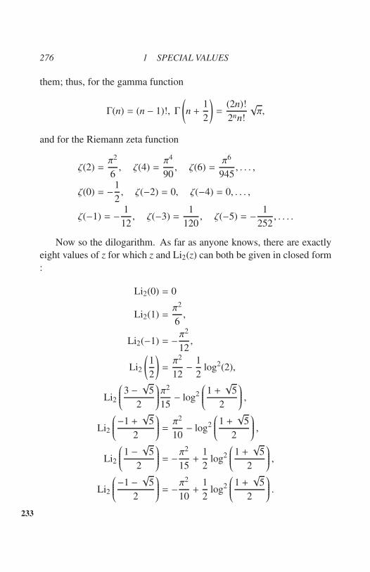
276 1 SPECIAL VALUES

them; thus, for the gamma function

Γ(n) = (n − 1)!, Γ

(n +

1

2

)=

(2n)!

2nn!

√π,

and for the Riemann zeta function

ζ(2) =π2

6, ζ(4) =

π4

90, ζ(6) =

π6

945, . . . ,

ζ(0) = −1

2, ζ(−2) = 0, ζ(−4) = 0, . . . ,

ζ(−1) = −1

12, ζ(−3) =

1

120, ζ(−5) = −

1

252, . . . .

Now so the dilogarithm. As far as anyone knows, there are exactly

eight values of z for which z and Li2(z) can both be given in closed form

:

Li2(0) = 0

Li2(1) =π2

6,

Li2(−1) = −π2

12,

Li2

(1

2

)=π2

12− 1

2log2(2),

Li2

3 −√

5

2

π2

15− log2

1 +√

5

2

,

Li2

−1 +

√5

2

=π2

10− log2

1 +√

5

2

,

Li2

1 −√

5

2

= −π2

15+

1

2log2

1 +√

5

2

,

Li2

−1 −

√5

2

= −π2

10+

1

2log2

1 +√

5

2

.

233

277

Let me describe a recent experience where these special values fig-

ures, and which admirably illustrates what I said about the bizarreness of

the occurrences of the dilogarithm in mathematics. From Bruce Berndt

via Henri Cohen I learned of a still unproved assertion in the Notebooks

of Srinivasa Ramanujan (Vol. 2, p. 289, formula (4)) : Ramanujan says

that, for q and x between 0 and 1,

q

x +q4

x +q8

x +q12

x+. . .

= 1 −qx

1 +q2

1 −q3x

1 +q4

1 −q5x

1+. . .

“very nearly.” He does not explain what this means, but a little ex-

perimentation shows that what is meant is that the two expressions are

numerically very close when q is near 1; thus for q = 0.9 and x = 0.5

one has

LHS = 0.7767340194. . . , RHS = 0.7767340180....

234

A graphical illustration of this is also shown.

LHS

RHS

1.5

1.0

0.5

0.2 0.4 0.6 0.8 1.00

LHS

RHS

0.2 0.6 0.8 1.00

1.5

1.0

0.5

The quantitative interpretation turned out as follows [9] : The dif-

ference between the left and right sides of Ramanujan’s equation is

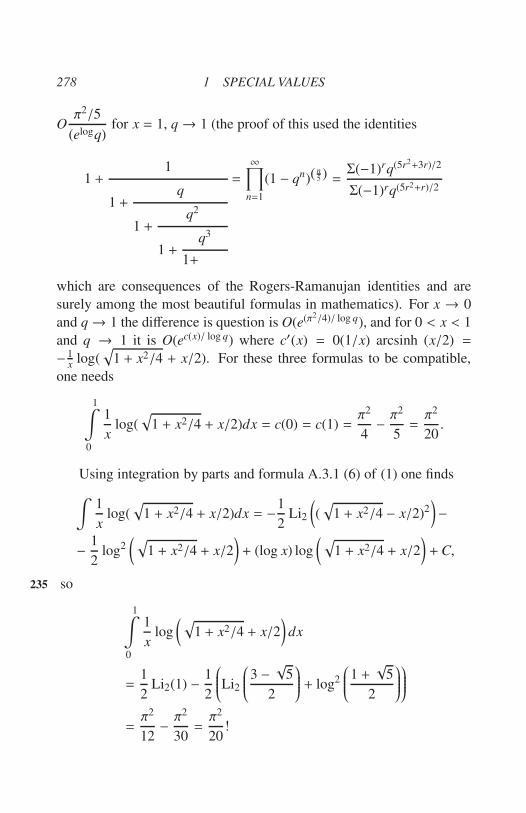
278 1 SPECIAL VALUES

Oπ2/5

(elogq)for x = 1, q→ 1 (the proof of this used the identities

1 +1

1 +q

1 +q2

1 +q3

1+

=

∞∏

n=1

(1 − qn)(n5 ) =

Σ(−1)rq(5r2+3r)/2

Σ(−1)rq(5r2+r)/2

which are consequences of the Rogers-Ramanujan identities and are

surely among the most beautiful formulas in mathematics). For x → 0

and q→ 1 the difference is question is O(e(π2/4)/ log q), and for 0 < x < 1

and q → 1 it is O(ec(x)/ log q) where c′(x) = 0(1/x) arcsinh (x/2) =

− 1x

log(√

1 + x2/4 + x/2). For these three formulas to be compatible,

one needs

1∫

0

1

xlog(

√1 + x2/4 + x/2)dx = c(0) = c(1) =

π2

4−π2

5=π2

20.

Using integration by parts and formula A.3.1 (6) of (1) one finds

∫1

xlog(

√1 + x2/4 + x/2)dx = −1

2Li2

((√

1 + x2/4 − x/2)2)−

−1

2log2

(√1 + x2/4 + x/2

)+ (log x) log

( √1 + x2/4 + x/2

)+C,

so235

1∫

0

1

xlog

( √1 + x2/4 + x/2

)dx

=1

2Li2(1) − 1

2

Li2

3 −√

5

2

+ log2

1 +√

5

2

=π2

12−π2

30=π2

20!

279

2 Functional equations In contrast to the paucity of special

values, the dilogarithm function satisfies a plethora of functional equa-

tions. To begin with, there are the two reflection properties

Li2(1/z) = −Li2(z) − (π2/6) − (1/2) log2(−z)

Li2(1 − z) = −Li2(z) + (π2/6) − log(z) log(1 − z).

Together they say that the six functions

Li2(z),Li2

(1

1 − z

),Li2

(z − 1

z

),−Li2

(1

z

),−Li2(1 − z),−Li2

(z

z − 1

)

are equal modulo elementary functions. Then there is the duplication

formula

Li2(z2),Li2

(1

1 − z

),Li2

(z − 1

z

),−Li2

(1

z

),−Li2(1 − z),−Li2

(z

z − 1

)

are equal modulo elementary functions. Then there is the duplication

formula

Li2(z2) = 2(Li2(z) + Li2(−z))

and more generally the “distribution property”

Li2(x) = n∑

zn=x

Li2(z) (n = 1, 2, 3, . . .).

Next, there is the two-variable, five-term relation

Li2(x) + Li2(y) + Li2

(1 − x

1 − xy

)+ Li2(1 − xy) + Li2

(1 − y

1 − xy

)

=π2

2− log(x) log(1 − x) − log(y) log(1 − y) + log

(1 − x

1 − xy

)log

(1 − y

1 − xy

)

which (in this or one of the many equivalent forms obtained by applying

the symmetry properties given above) was discovered and rediscovered

by Spence (1809). Abel (1827), Hill (1828), Kummer (1840), Schaef-

fer (1846), and doubtless others. (Despite appearances, this relation is 236

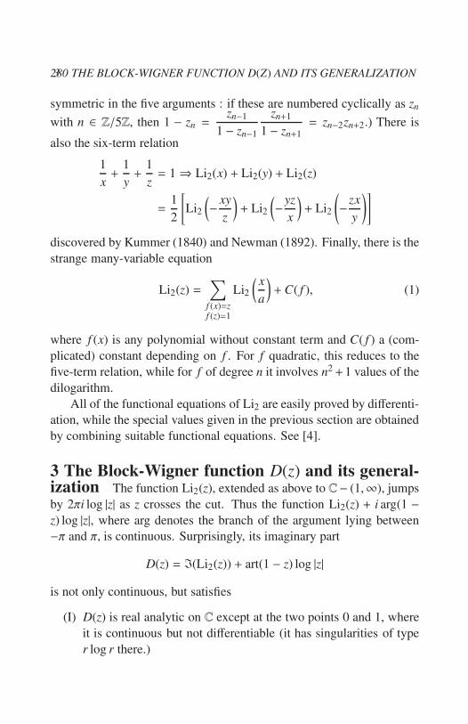
2803 THE BLOCK-WIGNER FUNCTION D(Z) AND ITS GENERALIZATION

symmetric in the five arguments : if these are numbered cyclically as zn

with n ∈ Z/5Z, then 1 − zn =zn−1

1 − zn−1

zn+1

1 − zn+1

= zn−2zn+2.) There is

also the six-term relation

1

x+

1

y+

1

z= 1⇒ Li2(x) + Li2(y) + Li2(z)

=1

2

[Li2

(− xy

z

)+ Li2

(−yz

x

)+ Li2

(−zx

y

)]

discovered by Kummer (1840) and Newman (1892). Finally, there is the

strange many-variable equation

Li2(z) =∑

f (x)=zf (z)=1

Li2

(x

a

)+C( f ), (1)

where f (x) is any polynomial without constant term and C( f ) a (com-

plicated) constant depending on f . For f quadratic, this reduces to the

five-term relation, while for f of degree n it involves n2+1 values of the

dilogarithm.

All of the functional equations of Li2 are easily proved by differenti-

ation, while the special values given in the previous section are obtained

by combining suitable functional equations. See [4].

3 The Block-Wigner function D(z) and its general-ization The function Li2(z), extended as above to C− (1,∞), jumps

by 2πi log |z| as z crosses the cut. Thus the function Li2(z) + i arg(1 −z) log |z|, where arg denotes the branch of the argument lying between

−π and π, is continuous. Surprisingly, its imaginary part

D(z) = I(Li2(z)) + art(1 − z) log |z|

is not only continuous, but satisfies

(I) D(z) is real analytic on C except at the two points 0 and 1, where

it is continuous but not differentiable (it has singularities of type

r log r there.)

281

0.2

0.4

0.60.8

0.9

1.0

0 1 2 3

Level Curves

of

237

The above graph shows the behaviour of D(z). (We have plotted the

level curves D(z) = 0, .2, .4, .6, .8, .9, 1.0 in the upper half-plane. The

values in the lower half-plane are obtained from D(z) = −D(z). The

maximum of D is 1.0149 . . ., attained at the point (1 + i√

3)/2.)

The function D(z), which was discovered by D. Wigner and S. Bloch

(cf. [1]), has many other beautiful properties. In particular :

(II) D(z), which is a real-valued function of C, can be expressed in

terms of a function of a single real variable, namely

D(z) =1

2

[D

(z

z

)+ D

(1 − 1/z

1 − 1/z

)+ D

(1/(1 − z)

1/(1 − z)

)](2)

which expresses D(z) for arbitrary complex z in terms of the func-

tion

D(eiθ) = I[Li2(eiθ)] =

∞∑

n=1

sin nθ

n2.

Note that the real part of Li2 on the unit circle is elementary : 238

∞∑

n=1

cos nθ

n2=π2

6−θ(2π − θ)

4for 0 ≤ θ ≤ 2π.)

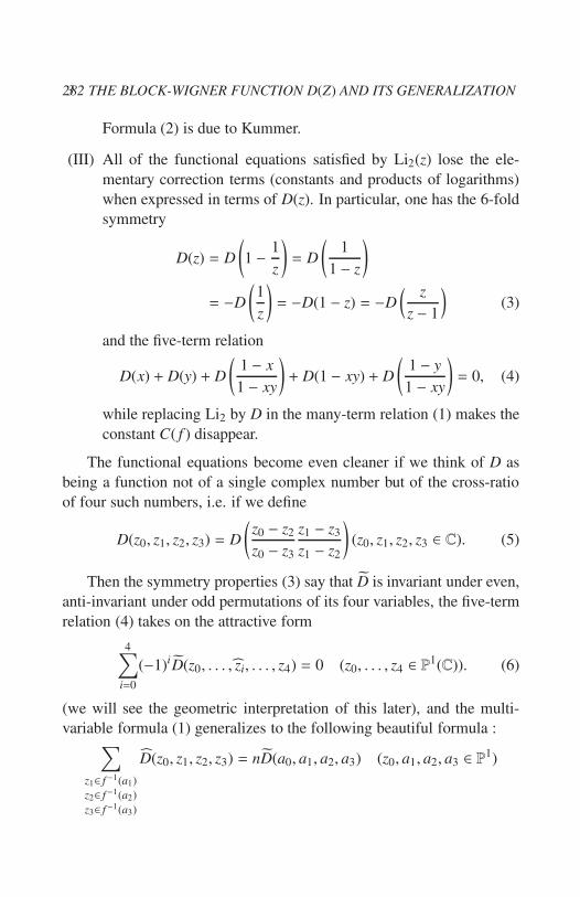
2823 THE BLOCK-WIGNER FUNCTION D(Z) AND ITS GENERALIZATION

Formula (2) is due to Kummer.

(III) All of the functional equations satisfied by Li2(z) lose the ele-

mentary correction terms (constants and products of logarithms)

when expressed in terms of D(z). In particular, one has the 6-fold

symmetry

D(z) = D

(1 −

1

z

)= D

(1

1 − z

)

= −D

(1

z

)= −D(1 − z) = −D

(z

z − 1

)(3)

and the five-term relation

D(x) + D(y) + D

(1 − x

1 − xy

)+ D(1 − xy) + D

(1 − y

1 − xy

)= 0, (4)

while replacing Li2 by D in the many-term relation (1) makes the

constant C( f ) disappear.

The functional equations become even cleaner if we think of D as

being a function not of a single complex number but of the cross-ratio

of four such numbers, i.e. if we define

D(z0, z1, z2, z3) = D

(z0 − z2

z0 − z3

z1 − z3

z1 − z2

)(z0, z1, z2, z3 ∈ C). (5)

Then the symmetry properties (3) say that D is invariant under even,

anti-invariant under odd permutations of its four variables, the five-term

relation (4) takes on the attractive form

4∑

i=0

(−1)iD(z0, . . . , zi, . . . , z4) = 0 (z0, . . . , z4 ∈ P1(C)). (6)

(we will see the geometric interpretation of this later), and the multi-

variable formula (1) generalizes to the following beautiful formula :∑

z1∈ f −1(a1)

z2∈ f −1(a2)

z3∈ f −1(a3)

D(z0, z1, z2, z3) = nD(a0, a1, a2, a3) (z0, a1, a2, a3 ∈ P1)

283

where f : P1 → P1 is a function of degree n and a0 = f (z0). (Equation239

(1) is the special case when f is a polynomial, so f −1(∞) is ∞ with

multiplicity n.)

Finally, we mention that a real-analytic function on P1(C)−0, 1,∞built up out of the polylogarithms in the same way as D(z) was con-

structed from the dilogarithm, has been defined by Ramakrishnan [6].

His function (slightly modified) is given by

Dm(z) = R

im+1

m∑

k=1

(− log |z|)m−k

(m − k)!Lik(z) − (log |z|)m

2m!

(so D1(z) = log |z1/2 − z−1/2|,D2(z) = D(z)) and satisfies

Dm

(1

z

)= (−1)m−1Dm(z),

∂

∂zDm(z) =

i

2z

(Dm−1(z) +

i

2

(−i log |z|)m−11 + z

(m − 1)! 1 − z

).

However, it does not seem to have analogues of the properties (II) and

(III) : for example, it is apparently impossible to express D3(z) for arbi-

trary complex z in terms of only the function D3(eiθ) =∑∞

n=1(cos nθ)/n3,

and passing from Li3 to D3 removes many but not all of the numerious

lower-order terms in the various functional equations of the trilogarithm,

e.g. :

D3(x) + D3(1 − x) + D3

(x

x − 1

)

= D3(1) +1

12log |x(1 − x)| log

∣∣∣∣∣x

(1 − x)2

∣∣∣∣∣ log

∣∣∣∣∣∣x2

1 − x

∣∣∣∣∣∣ ,

D3

(x(1 − y)2

y(1 − x)2

)+ D3(xy) + D3

(x

y

)− 2D3

(x

y

1 − y

1 − x

)

− 2D3

(x(1 − y)

x − 1

)− 2D3

(y(1 − x)

y − 1

)− 2D3

(1 − y

1 − x

)

− 2D3(x) − 2D3(y) = 2D3(1) −1

4log |xy| log

∣∣∣∣∣x

y

∣∣∣∣∣ log

∣∣∣∣∣∣x

y

(1 − y)2

(1 − x)2

∣∣∣∣∣∣ .

284 4 VOLUMES OF HYPERBOLIC 3-MANIFOLDS. . .

Nevertheless, these higher Bloch-Wigner functions do occur. In study- 240

ing the so-called “Heegner points” on modular curves, B. Gross and I

had to study for n = 2, 3, . . . “higher weight Green’s functions” for H/Γ

(H = complex upper half-plane, Γ = S L2(Z) or a congruence subgroup).

These are functions Gn(z1, z2) = GH/Γn (z1, z2) defined on H/Γ×H/Γ, real-

analytic in both variables except for a logarithmic singularity along the

diagonal z1 = z2, and satisfying ∆z1Gn = ∆z2

Gn = n(n − 1)Gn, where

∆z = y2(∂2/∂x2+∂2/∂y2) is the hyperbolic Laplace operator with respect

to z = x + iy ∈ H. They are obtained as

GG/Γn (z1, z2) =

∑

γ∈ΓGHn (z1, γz2)

where GHn is defined analogously to G

G/Γn but with H/Γ replaced by H.

The functions GHn (n = 2, 3, . . .) are elementary, e.g.,

GH

2(z1, z2) =

(1 +|z1 − z2|2

2y1y2

)log|z1 − z2|2

|z1 − z2|2+ 2.

In between GHn and G

H/Γn are the functions G

H/Γn = Σr∈ZG

Hn (z1, z2 + r).

It turns out [10] that these are expressible in terms of the Dm(m =

1, 3, . . . , 2n − 1), e.g.,

GH/Z

2(z1, z2) =

1

4π2y1y2

(D3(e2πi(z1−z2)) + D3(e2πi(z1−z2))

+y2

1+ y2

2

2y1y2

(D1(e2πi(z1−z2)) + D1(e2πi(z1−z2)))

I do not know the reasons for this connection.

241

4 Volumes of Hyperbolic 3-manifolds. . . The diloga-

rithm occurs in connection with measurement of volumes in Euclidean,

spherical, and hyperbolic geometry. We will be concerned with the last

of these. Let H3 be the Lobachevsky space (space of non- Euclidean

solid geometry). We will use the half-space model, in which H3 is rep-

resented by C × R+ with the standard hyperbolic metric in which the

285

geodesics are either vertical lines or semicircles in vertical planes with

endpoints in C × 0 and the geodesic planes are either vertical planes

or else hemispheres with boundary in C × 0. An ideal tetrahedron is a

tetrahedron whose vertices are all in ∂H3 = C ∪ ∞ = P1(C). Let ∆ be

such a tetrahedron. Although the vertices are at infinity, the (hyperbolic)

volume is finite. It is given by

Vol(∆) = D(z0, z1, z2, z3), (7)

where z0, . . . , z3 ∈ C are the vertices of ∆ and D is the function defined

in (5). In the special case that three of the vertices of ∆ are ∞, 0, and 1,

equation (7) reduces to the formula (due essentially to Lobachevsky)

Vol(∆) = D(z). (8)

Volume

0 1

Volume

In fact, equations (7) and (8) are equivalent since any 4-tuple of

points z0, . . . , z3 can be brought into the form ∞, 0, 1, z by the action

of some element of S L2(C) on P1(C), and the group S L2(C) acts on H3

by isometries.

The (anti-) symmetry properties of D under permutations of the zi 242

are obvious from the geometric interpretation (7), since renumbering the

vertices leaves ∆ unchanged but may reverse its orientation. Formula

(6) is also an immediate consequence of (7), since the five tetrahedra

286 4 VOLUMES OF HYPERBOLIC 3-MANIFOLDS. . .

spanned by four at a time of z0, . . . , z4 ∈ P1(C), counted positively or

negatively as in (6), add up algebraically to the zero 3-cycle.

The reason that we are interested in hyperbolic tetrahedra is that

these are the building blocks of hyperbolic 3-manifolds, which in turn

(according to Thurston) are the key objects for understanding three-

dimensional geometry and topology. A hyperbolic 3-manifold is a 3-

dimensional riemannian manifold M which is locally modelled on (i.e.,

isometric to portions of) hyperbolic 3-space H3; equivalently, it has con-

stant negative curvature −1. We are interested in complete oriented

hyperbolic 3-manifolds which have finite volume (they are then either

compact or have finitely many “cusps” diffeomorphic to S 1 × S 1 ×R+).

Such a manifold can obviously be triangulated into small geodesic sim-

plices which will be hyperbolic tetrahedra. Less obvious is that (possi-

bly after removing from M a finite number of closed geodesics) there

is always a triangulation into ideal tetrahedra (the part of such a tetra-

hedron going out towards a vertex at infinity will then either tend to a

cusp of M or else spiral in around one of the deleted curves). Let these

tetrahedra be numbered ∆1, . . . ,∆n and assume (after an isometry of H3

if necessary) that the vertices of ∆v are at∞, 0, 1 and zv. Then

Vol(M) =

n∑

v=1

D(zv). (9)

Of course, the numbers zv are not uniquely determined by ∆v since they

depend on the order in which the vertices were sent to ∞, 0, 1, zv, but

the non-uniqueness consists (since everything is oriented) only in re-

placing zv by 1 − 1/zv or 1/(1 − zv) and hence does not affect the value

of D(zv).

One of the objects of interest in the study of hyperbolic 3-manifolds

is the “volume spectrum”

Vol = Vol(M)|M hyperbolic 3-manifold ⊂ R+.

From the work of Jørgensen and Thurston one knows the Vol is a count-

able and well-ordered subset of R+ (i.e. every subset has a smallest

287

element), and its exact nature is of considerable interest both in topol-

ogy and number theory. Equation (9) as it stands says nothing about

this set since any real number can be written as a finite sum of values 243

D(z), z ∈ C. However, the parameters zv of the tetrahedra triangulating

a complete hyperbolic 3-manifold satisfy an extra relation, namely

n∑

v=1

zv ∧ (1 − zv) = 0, (10)

where the sum is taken in the abelian group ∧2C× (the set of all formal

linear combinations x ∧ y, x, y ∈ C×, subject to the relations x ∧ x = 0

and (x1x2) ∧ y = x1 ∧ y + x2 ∧ y). (This follows from assertions in [3]

or form Corollary 2.4 of [5] applied to suitable x and y). Now (9) does

give information about Vol because the set of numbers Σnv=1

D(zv) with zv

satisfying (10) is countable. This fact was proved by Bloch [1]. To make

a more precise statement, we introduce the Bloch group. Consider the

abelian group of formal sums [z1] + · · · + [zn] with z1, . . . , zn ∈ C× − 1satisfying (10). As one easily checks, it contains the elements

[x]+

[1

x

], [x]+ [1− x], [x]+ [y]+

[1 − x

1 − xy

]+ [1− xy]+

[1 − y

1 − xy

](11)

for all x and y in C× − 1 with xy , 1, corresponding to the symmetry

properties and 5-term relation satisfied by D(·). The Block group is

defined as

BC = [z1] + · · · + [zn] satisfying (10)/(subgroup generated by

the elements (11))

(12)

(this is slightly different from the usual definitions). The definition of the

Block group in terms of the relations satisfied by D(·) makes it obvious

that D extends to a linear map D : BC + R by [z1] + · · · + [zn] 7→D(z1) + · · · + D(zn), and Bloch’s result (related to Mostow rigidity) says

that the set D(BC) coincides with D(BQ

) (where BQ

is defined by (12)

but with the zv lying in Q×− 1). Thus D(BC) is countable, and (9) and

(10) imply that Vol is contained in this countable set. The structure of

BQ

which is very subtle, will be discussed below.

288 5 . . . AND VALUES OF DEDEKIND ZETA FUNCTIONS

We give an example of a non-trivial element of the Bloch group. For

convenience, set α =1 −√−7

2, β =

−1 −√−7

2. Then

2

1 +√−7

2

∧

1 −√−7

2

+−1 +

√−7

4

∧

5 −√−7

4

2(−β) ∧ α +(1

β

)∧

(α2

β

)= β2 ∧ α − β ∧ α2 = 2 · β ∧ α − 2 − ·β ∧ α = 0,

so244

2

1 +√−7

2

+−1 +

√−7

4

∈ BC. (13)

This example should make it clear why non-trivial elements of BC can

only arise from algebraic numbers — the key relations 1 + β = α and

1 − β−1 = α2/β above forced α and β to be algebraic.

5 . . . and values of Dedekind zeta functions Let F be

an algebraic number field, say of degree N over O. Among its most im-

portant invariants are the discriminant d, the numbers r1 and r2 of real

and imaginary archimedean valuations, and the Dedekind zeta-function

ζF(s). For the non-number-theorist we recall the (approximate) defini-

tions. The field F can be represented as Q(α) where α is a root of an

irreducible monic polynomial f ∈ Z[x] of degree N. The discriminant

of f is an integer d f and d is given by c−2d f for some natural number

c with c2|d f . The polynomial f , which is irreducible over Q, in general

becomes reducible over R, where it splits into r1 linear and r2 quadratic

factors (thus r1 ≥ 0, r2 ≥ 0, r1 + 2r2 = N). It also in general becomes

reducible when it is reduced modulo a prime p, but if p ∤ d f then its

irreducible factors modulo p are all distinct, say r1,p linear factors, r2,p

quadratic ones, etc. (so r1,p + 2r2,p + · · · = N). Then ζF(s) is the Dirich-

let series given by an Euler product ΠpZp(p−s)−1 where Zp(t) for p ∤ d f

is the monic polynomial (1 − t)r1,p(1 − t2)r2,p . . . of degree N and ZP(t)

for p|d f is a certain monic polynomial of degree ≤ N. Thus (r1, r2) and

ζF(s) encode the information about the behaviour of f (and hence F)

over the real and p-adic numbers, respectively.

289

As an example, let F be an imaginary quadratic field O(√−a) with

a ≥ 1 squarefree. Here N = 2, d = −a or −4a, r1 = 0, r2 = 1.

The Dedekind zeta function has the form∑

n≥1r(n)n−s where r(n) counts

representations of n by certain quadratic forms of discriminant d; it can

also be represented as the product of the Riemann zeta function ζ(s) =

ζ(s)

Owith an L-series L(s) =

∑n≥1

(dn

)n−s where

(dn

)is a symbol taking the 245

values ±1 or 0 and which is periodic of period |d| in n. Thus for a = 7

ζQ(√−7)

(s) =1

2

∑

(x,y),(0,0)

1

(x2 + xy + 2y2)s

=

∞∑

n=1

n−s

∞∑

n=1

(−7

n

)n−s

where(−7n

)is +1 for n ≡ 1, 2, 4(mod 7), −1 for n ≡ 3, 5, 6(mod 7), and

0 for n ≡ 0(mod 7).

One of the questions of interest is the evaluation of the Dedekind

zeta function at suitable integer arguments. For the Riemann zeta func-

tion we have the special values cited at the beginning of this paper.

More generally, if F is totally real (i.e., r1 = N, r2 = 0), then a the-

orem of Siegel and Klingen implies that ζF(m) for m = 2, 4, . . . equals

πmN/√

d times a rational number. If r2 > 0, then no such simple result

holds. However, in the case F = Q(√−a), then using the representation

ζF(s) = ζ(s)L(s) and the formula ζ(2) = π2/6 and writing the periodic

function (d/n) as a finite linear combination of terms e2πin d, we obtain

ζF(2) =π2

6√|d|

|d|−1∑

n=1

(d

n

)D(e2πin d) (F imaginary quadratic),

e.g.,

ζQ(√−7)

(2) =π2

3√

7

(D(e2πi/7) + D(e4πi/7) − D(e6πi/7)

)

Thus the values of ζF(2) for imaginary quadratic fields can be expressed

in closed form in terms of values of the Bloch-Wigner function D(z) at

algebraic arguments z.

290 5 . . . AND VALUES OF DEDEKIND ZETA FUNCTIONS

By using the ideas of the last section we can prove a much stronger

statement. Let O denote the ring of integers of F (this is the Z-lattice in

C spanned by 1 and√−a or (1 +

√−a)/2, depending whether d = −4a

or d = −a). Then the group Γ = S L2(O) is a discrete subgroup of

S L2(C) and therefore acts on hyperbolic space H3 by isometries. A

classical result of Humbert gives the volume of the quotient space H3/Γ

as |d|3/2 × ζF(2)/4π2. On the other hand, H3/Γ (or, more precisely, a246

certain covering of it of low degree) can be triangulated into ideal tetra-

hedra with vertices belonging to P1(F) ⊂ P1(C), and this leads to a

representation

ζF(2) =π2

3|d|3/2∑

v

nvD(zv)

with nv in Z and zv in F itself rather than in the much larger field

Q(e2πi d)([8], Theorem 3). For instance, in our example F = Q(√−7)

we find

ζF(2) =4π2

21√

7

2D

1 +√−7

2

+ D

−1 +

√−7

4

.

This equation together with the fact that ζF(2) = 1.89484144897 . . . , 0

implies that the element (13) has infinite order in BC.

In [8], it was pointed out that the same kind of argument works

for all number fields, not just imaginary quadratic ones. If r2 = 1 but

N > 2 then one can again associate to F (in many different ways) a dis-

crete subgroup Γ ⊂ S L2(C) such that Vol(H3/Γ) is a rational multiple

of d|1/2ζF(2) × π2(1−N). This manifold H3/Γ is now compact, so the de-

composition into ideal tetrahedra is a little less obvious than in the case

of imaginary quadratic F, but by decomposing into non-ideal tetrahedra

(tetrahedra with vertices in the interior of H3) and writing these as dif-

ferences of ideal ones, it was shown that the volume is an integral linear

combination of values of D(z) with z of degree at most 4 over F. For

F completely arbitrary there is still a similar statement, except that now

one gets discrete groups Γ acting on Hr2

3; the final result ([8], Theorem 1)

is that |d|1/2 × ζF(2)/π2(r1+r2) is a rational linear combination of r2-fold

products D(z(1)) . . .D(z(r2)) with each z(i) of degree ≤ 4 over F (more

291

precisely, over the ith complex embedding F(i) of F, i.e. over the sub-

field Q(α(i)) of C where α(i) is one of the two roots of the ith quadratic

factor of f (x) over R).

But in fact much more is true : the z(i) can be chosen in F(i) itself

(rather than of degree 4 over this field), and the phrase “rational linear

combination of r2-fold products” can be replaced by “rational multiple

of an r2 × r2 determinant.” We will not attempt to give more than a very

sketchy account of why this is true, lumping together work of Wigner,

Bloch, Dupont, Sah, Levine, Merkuriev, Suslin, . . . for the purpose (ref-

erences are [1], [3], and the survey paper [7]). This work connects the

Bloch group defined in the last section with the algebraic K-theory of 247

the underlying field; specifically, the group1 BF is equal, at least after

tensoring it with O, to a certain quotient Kind3

(F) of K3(F). The exact

definition of Kind3

(F) is not relevant here. What is relevant is that this

group has been studied by Borel [2], who showed that it is isomorphic

(modulo torsion) to Zr2 and that there is a canonical homomorphism,

the “regulator mapping,” from it into Rr2 such that the co-volume of

the image in a non-zero rational multiple of |d|a/2ζF(2)/π2r1+2r2 ; more-

over, it is known that under the identification of Kind3

(F) with BF this

mapping corresponds to the composition BF → (BC)r2D−→ Rr2 , where

the first arrow comes from using the r2 embeddings F ⊂ C(α → α(i)).

Putting all this together gives the following beautiful picture : The group

BF/torsion, is isomorphic to Zr2 . Let ζ1, . . . , ζr2by any r2 linearly

independent elements of it, and form the matrix with entires D(ζ(i)

j),

(i, j = 1, . . . , r2). Then the determinant of this matrix is a non-zero ra-

tional multiple of |d|1/2ζF(2)/π2r1+2r2 . If instead of taking any r2 linearly

independent elements we choose the ζ j to be a basis of BF/torsion,then this rational multiple (chosen positively) is an invariant of F, inde-

pendent of the choice of ζ j. This rational multiple is then conjecturally

related to the quotient of the order of K3(F)torsion by the order of the

1It should be mentioned that the definition of BF which we gave for F = C or Q

must be modified slightly when F is a number field because F× is no longer divisible;

however, this is a minor point, affecting only the torsion in the Bloch group, and will be

ignored here.

292 5 . . . AND VALUES OF DEDEKIND ZETA FUNCTIONS

finite group K2(OF) where OF denotes the ring of integers of F (Licht-

enbaum conjectures).

This all sounds very abstract, but it is fact not. There is a reasonably

efficient algorithm to produce many elements of BF for any number

field F. If we do this, for instance, for F an imaginary quadratic field,

and compute D(ζ) for each element ζ ∈ BF which we find, then after

a while we are at least morally certain of having identified the lattice

D(BF) ⊂ R exactly (after finding k elements at random, we have only

about one chance in 2k of having landed in the same non-trivial sublat-

tice each time). By the results just quoted, this lattice is generated by a

number of the form κ|d|3/2ζF(2)/π2 with κ rational, and the conjecture

referred to above says that κ should have the form 32T

where T is the or-

der of the finite group K2(OF), at least for d < −4 (in this case the order

of K3(F)torsion is always 24). Calculations done by H. Gangl in Bonn for

several hundred imaginary quadratic fields support this; the κ he found

all have the form 32T

for some integer T and this integer agrees with the248

order of K2(OF) in the few cases where the latter is known. Here is a

small excerpt from his tables :

|d| 7 8 11 15 19 20 23 24 31 35 39 40 . . . 303 472 479 491 555 583

T 2 1 1 2 1 1 2 1 2 2 6 1 . . . 22 5 14 13 28 34

(the omitted values contain only the primes 2 and 3; 3 occurs whenever

d ≡ 3(mod 9) and there is also some regularity in the powers of 2 occur-

ring). Thus one of the many virtues of the mysterious dilogarithm is that

it gives, at least conjecturally, an effective way of calculating the orders

of certain groups in algebraic K-theory!

To conclude, we mention that Borel’s work connects not only

Kind3

(F) and ζF(2) but more generally Kind2m−1

(F) and ζF(m) for any inte-

ger m > 1. No elementary description of the higher K-groups analogous

to the description of K3 in terms of B is known, but one can at least spec-

ulate that these groups and their regulator mappings may be related to

the higher polylogarithms and that, more specifically, the value of ζF(m)

is always a simple multiple of a determinant (r2×r2 or (r1+r2)×(r1+r2)

depending whether m is even or odd) whose entries are linear combina-

tions of values of the Bloch-Wigner-Ramakrishnan function Dm(z) with

REFERENCES 293

arguments z ∈ F. As the simplest case, one can guess that for a real

quadratic field F the value of ζF(3)/ζ(3) = L(3), where L(s) is a Dirich-

let L-Function of a real quadratic character of period d) is equal to d−5/2

times a simple rational linear combination of differences D3(x)−D3(x′)with x ∈ F, where x′ denotes the conjugate of x over Q. Here is one

(numerical) example of this :

2−555/2ζQ(√

5)(3)/ζ(3) = D3

1 +√

5

2

− D3

1 −√

5

2

−

− 1

3[D3(2 +

√5) − D3(2 −

√5)]

(both sides are equal approximately to 1.493317411778544726). I have

found many other examples, but the general picture is not yet clear.

References

[1] S. Bloch : Applications of the dilogarithm function in algebraic 249

K-theory and algebraic geometry, in : Proc. of the International

Symp. on Alg . Geometry, Kinokuniya, Tokyo, 1978.

[2] A. Borel : Commensurability classes and volumes of hyperbolic

3-manifolds, Ann. Sc. Norm. Sup. Pisa, 8 (1981) pp. 1-33.

[3] J. L. Dupont and C. H. Sah : Scissors congruences II, J. Pure and

Applied Algebra, 25 (1982), 159-195.

[4] L. Lewin : Polylogarithms and associated functions (title of orig-

inal 1958 edition : Dilogarithms and associated functions). North

Holland, New York, 1981.

[5] W. Neumann and D. Zagier : Volumes of hyperbolic 3-manifolds,

Topology, 24 (1985), 307-332.

[6] D. Ramakrishnan : Analogs of the Bloch-Wigner function for

higher polylogarithms, Contemp. Math., 55 (1986), 371-376.

294 REFERENCES

[7] A. A. Suslin : Algebraic K-theory of fileds, in : Proceedings of the

ICM Berkeley 1986 A.M.S. (1987), 222-244.

[8] D. Zagier : Hyperbolic manifolds and special values of Dedekind

zeta-functions, Invent. Math., 83 (1986), 285-301.

[9] D. Zagier : On an approximate identity of Ramanujan, Proc. Ind.

Acad. Sci. (Ramanujan Centenary Volume) 97 (1987), 313-324.

[10] D. Zagier : Green’s functions of quotients of the upper half-plane

(in preparation.)

Max-Planck-Institut fur Mathematik,

Gottfried-Claren-Straße 26, D-5300 Bonn, FRG.

and

Department of Mathematics,

University of Maryland,

College Park, Maryland 20742, USA.

This book contains original papers presented at

the Srinivasa Ramanujan Birth Centenary Inter-

national Colloquium on Number Theory and Re-

lated Topics held at the Tata Institute of Funda-

mental Reserach in January 1988.