Number Theory, Special Functions, Matrices. 2/16/2004Discrete Mathematics for Teachers, UT Math 504, Lecture 06 2 Number Theory Basic Notation and Terms:

Number Theory, Special Functions, Matrices

2/16/2004 Discrete Mathematics for Teachers, UT Math 504, Lecture 06

2

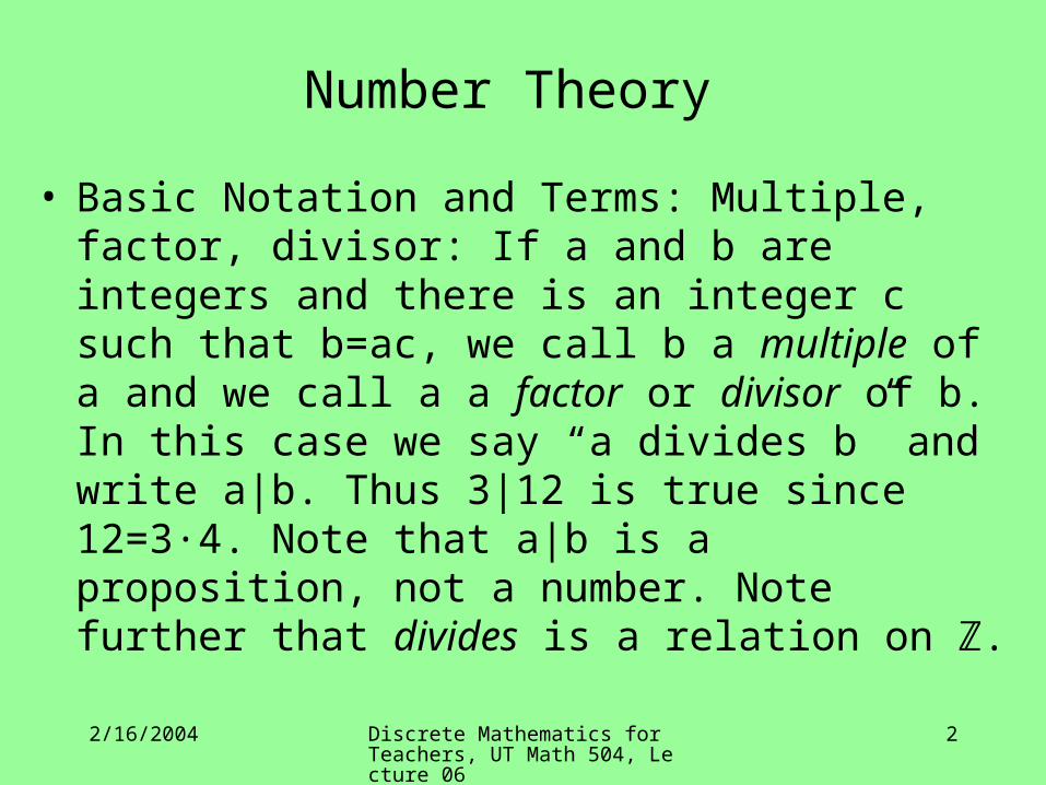
Number Theory

• Basic Notation and Terms: Multiple, factor, divisor: If a and b are integers and there is an integer c such that b=ac, we call b a multiple of a and we call a a factor or divisor of b. In this case we say “a divides b” and write a|b. Thus 3|12 is true since 12=3∙4. Note that a|b is a proposition, not a number. Note further that divides is a relation on .ℤ


3

Number Theory

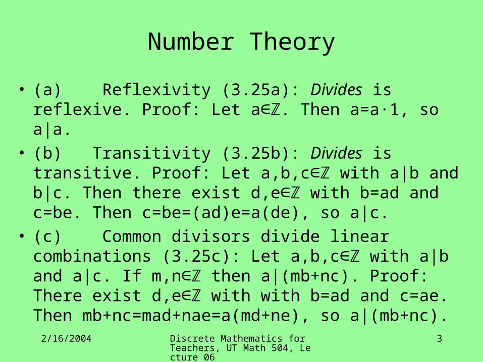
• (a) Reflexivity (3.25a): Divides is reflexive. Proof: Let a . Then a=a∙1, so a|a.∈ℤ

• (b) Transitivity (3.25b): Divides is transitive. Proof: Let a,b,c with a|b and b|c. Then there exist d,e with ∈ℤ ∈ℤb=ad and c=be. Then c=be=(ad)e=a(de), so a|c.

• (c) Common divisors divide linear combinations (3.25c): Let a,b,c∈ℤ with a|b and a|c. If m,n∈ℤ then a|(mb+nc). Proof: There exist d,e∈ℤ with with b=ad and c=ae. Then mb+nc=mad+nae=a(md+ne), so a|(mb+nc).


4

Number Theory

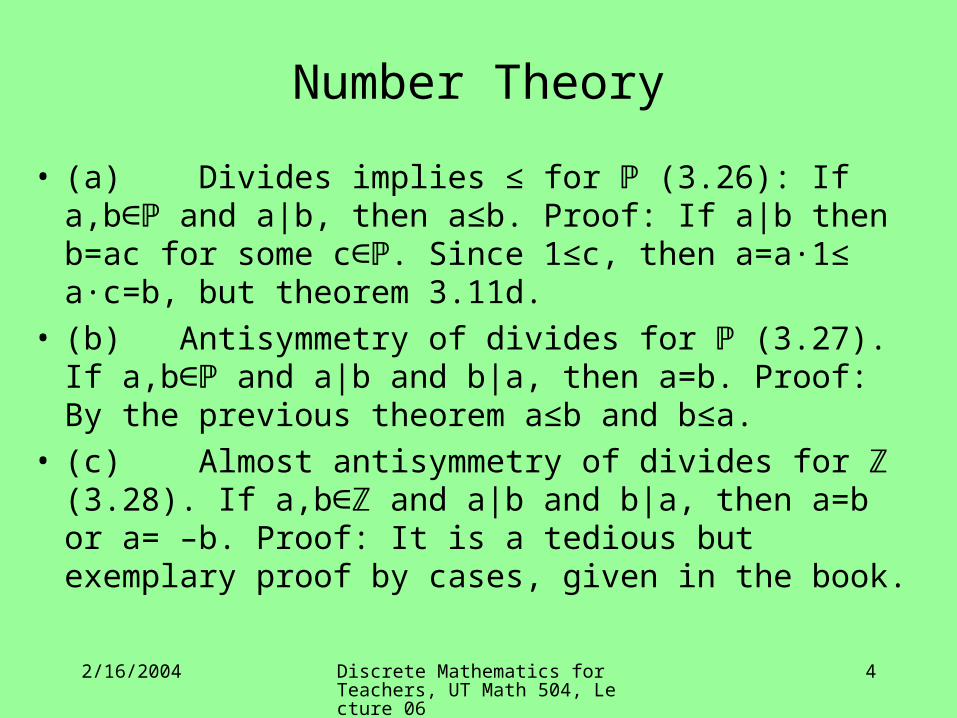
• (a) Divides implies ≤ for ℙ (3.26): If a,b∈ℙ and a|b, then a≤b. Proof: If a|b then b=ac for some c∈ℙ. Since 1≤c, then a=a∙1≤ a∙c=b, but theorem 3.11d.

• (b) Antisymmetry of divides for ℙ (3.27). If a,b∈ℙ and a|b and b|a, then a=b. Proof: By the previous theorem a≤b and b≤a.

• (c) Almost antisymmetry of divides for ℤ (3.28). If a,b∈ℤ and a|b and b|a, then a=b or a= –b. Proof: It is a tedious but exemplary proof by cases, given in the book.


5

Number Theory

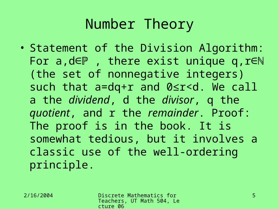
• Statement of the Division Algorithm: For a,d∈ℙ , there exist unique q,r∈ℕ (the set of nonnegative integers) such that a=dq+r and 0≤r<d. We call a the dividend, d the divisor, q the quotient, and r the remainder. Proof: The proof is in the book. It is somewhat tedious, but it involves a classic use of the well-ordering principle.


6

Number Theory

• Recall doing long division with remainder in third grade. The division algorithm guarantees that every such division problem has a quotient and remainder (smaller than the divisor) and that they are unique. So, for instance, if we divide 100 by 7 we get a quotient of 14 and a remainder of 2 since 100=7∙14+2.


7

Number Theory

• The division algorithm says, in essence that given a fixed divisor d we can uniquely describe every positive integer a by how far it is above the nearest smaller multiple of d. Not surprisingly this distance is always smaller than d. For instance, every positive integer is a multiple of 4 or is 1, 2, or 3 more than a multiple of 4.


8

Number Theory

• It works just as well to allow the dividend, divisor, and quotient to be integers (not just positive/nonnegative integers) so long as the divisor is nonzero. It is also possible to set other criteria for the remainder (for instance, to make |r| as small as possible). The key is that q and r must still be uniquely determined. For instance, if we divide –42 by 10 we can get a quotient of –5 with remainder 8 or we can get a quotient of –4 with a remainder of –2 depending on where we require the remainder to lie.


9

Number Theory

• As unassuming as this result appears, it is hard to overestimate the value of the division algorithm. It justifies many important results in elementary number theory.


10

Number Theory

• Definition of Common Divisor: A common divisor of integers a and b is an integer that divides them both. The text requires common divisors to be positive. For instance 2 and 3 are common divisors of 12 and 18.


11

Number Theory

• Definition of Greatest Common Divisor (gcd): The number d is the greatest common divisor of integers a and b if d is a common divisor and every other common divisor divides d. In this case we write d=gcd(a,b). More advanced texts simply write d=(a,b). This plainly implies that d is the largest of the common divisors of a and b. For instance 6 is the greatest common divisor of 12 and 18 since the common divisors 1, 2, 3, and 6 all divide 6.


12

Number Theory

• GCD is unique (3.32) Proof: If c and d are greatest common divisors of a and b, then c and d divide each other. Thus c=d.

• GCD is a linear combination (3.33): If d=gcd(a,b), then there are integers m and n such that d=ma+nb. In fact d is the smallest positive integer expressible as a linear combination of a and b. Proof: The proof is in the book. Please read it. It is a classic application of the division algorithm and the well-ordering principle.


13

Number Theory

• GCD divides the remainder (3.34). Let a,b ∈ ℤ with a=bq+r by the division algorithm. Then every common divisor of b and r also divides a. Rearranging we see r=a–bq, so every common divisor of a and b also divides r. In particular gcd(a,b)|r. In fact, gcd(a,b)=gcd(b,r).


14

Number Theory

• A divisor of a product divides one of the factors if the divisor is relatively prime to the other factor (3.35): If a,b,c∈ℤ with gcd(a,b)=1 (in this case we say a and b are relatively prime) and a|bc, then a|c. Proof: There exist integers m and n with ma+nb=gcd(a,b)=1. Multiply by c to get mac+nbc=c. Since a divides each of the terms on the left of this equation (a|mac and a|nbc, since a|bc), then a|c. This is another standard use of the division algorithm.


15

Number Theory

• Definition of Common Multiple: A common multiple of integers a and b is an integer m such that a|m and b|m. The text requires m to be positive. For instance some common multiples of 2 and 3 are 6, 12, 18, etc.

• Definition of Least Common Multiple (lcm): A common multiple m of integers a and b is the least common multiple of a and b if it divides every other common multiple. Clearly this does mean that every common multiple of a and b is at least as large as m. We denote it by lcm(a,b). For instance lcm(2,3)=6.


16

Number Theory

• Relationship of gcd and lcm (3.51 from the next section)): If a and b are positive integers, then ab=gcd(a,b)∙lcm(a,b). The proof is not particularly enlightening and is in the book.


17

Number Theory

• Definition of Prime and Composite: Throughout this section we deal only with positive integers: The number 1 is neither prime nor composite. A number a is prime if it is bigger than 1 and has only 1 and itself for factors. All other positive integers are composite.


18

Number Theory

• A composite number has a prime no larger than its square root (3.42). Proof: Let a be composite, and let p be its smallest factor besides 1. Suppose b is a factor of p that is not equal to p (a proper factor of p). Since p|a, then b|a. Since b|p, then b≤p. Thus b is a factor of a smaller than p. The only such factor is 1. Therefore p has only p and 1 as factors and is, thus, prime. Now suppose a=pq. Since p≥b, we know a=pq≥p∙p=p2, so p is no larger than the square root of a.


19

Number Theory

• Infinitude of primes (3.41): There are infinitely many primes. Proof (by contradiction): Assume not. Then there is a finite list of primes. Multiply them all together, add 1, and call the result a. Since a is bigger than every number in the list of primes, a is composite. By the previous theorem it has a prime factor. But if we divide a by one of the primes, there is a remainder of 1 by the construction of a, so no prime divides a. This is a contradiction, so there are infinitely many primes. (Note that the book gets theorems 3.41 and 3.42 in the wrong order since 3.41 depends on 3.42). As the book notes, this proof was known to Euclid.


20

Number Theory

• Existence of prime factorizations (3.43): Every positive integer is a product of primes. The book gives a standard proof using strong induction. Note by the way that a prime is itself the product of one prime (itself) and 1 is the product of no primes (By convention the product of no factors is 1).

• A prime dividing a product divides one of the factors (3.44, 3.45): If a prime p divides ab, then p|a or p|b. Proof. Suppose p does not divide a. Then the only common divisor of p and a is 1, so gcd(p,a)=1. That is, p and a are relatively prime. By Theorem 3.35, p|b.


21

Number Theory• A prime dividing a product of primes equals one of the primes

(3.46). This follows easily from the previous result.

• Every positive integer has a unique factorization into primes (3.47, 3.48). We already know the factorization exists. These theorems show that it is unique. The proof is a standard, somewhat tedious induction argument on the number of prime factors. It can also be somewhat tedious to define unique, even though the intent is obvious. This result leads to so many others that it is commonly called the Fundamental Theorem of Arithmetic; it is an ancient result with a proof appearing in Euclid. By the way, this result is not unique to the integers; it holds in some abstract rings which are naturally knows as unique factorization domains.


22

Number Theory

• A multiple has all the prime factors of its divisor to powers at least as high as those in the divisor (3.49). The book states this more precisely. The result seems obvious. The proof seems a little tedious, following the lines of the proof of unique prime factorization.

• A gcd has all the common primes to the minimum power of the two factors. An lcm has all the primes to the maximum power of the two factors. (3.50) When I was in school, these were the standard (indeed the only) means taught for finding gcd’s and lcm’s. They work well for numbers of modest size, but the Euclidean Algorithm (do you know it?) is much easier once the numbers become large.


23

Number Theory• Definition of congruence modulo n: Let a,b,n be integers

with n positive. We say say a is congruent to b modulo n and write a≡b (mod n) if n|(a–b). It is equivalent to say that a and b leave the same remainder when divided by n. For instance 23≡9 (mod 7), since 23–9=14=2∙7 or equivalently since 23 and 9 both leave a remainder of 2 when divided by 7.


24

Number Theory

• Definition of ℤ n: the integers modulo n: As appears

below, congruence modulo n is an equivalence relation. The set of equivalence classes under this equivalence relation is denoted ℤ n. As we have discussed before, for

instance, ℤ3={[0],[1],[2]}. Note that the numbers 0,1,

and 2 are the three possible remainders when dividing integers by 3.


25

Number Theory

• Congruence is an equivalence relation: Proof: Note a–a=0=n∙0, so n|(a–a) and a≡a (mod n) and congruence is reflexive. It is easy to see that ≡ is also symmetric and transitive using simple properties of divisibility.


26

Number Theory• Congruence preserves addition and multiplication

(3.55a). If a≡b (mod n) and c≡d (mod n), then (a+c)≡(b+d) (mod n) and ac≡bd (mod n). Proof: (a+c)–(b+d)=(a–b)+(c–d). By assumption n divides a–b and c–d, so n divides their sum. The proof for multiplication is similar but involves a little algebraic trick: ab–cd=ab–bc+bc–cd=(a–c)b+c(b–d). Thus since 23≡9 (mod 7) and –2≡5 (mod 7), then 21≡14 (mod 7) and –46≡45 (mod 7)


27

Number Theory

• Congruence modulo a product means congruence modulo each factor (3.55b). For instance 23≡2 (mod 21), so 23≡2 (mod 7) and 23≡2 (mod 3). The proof is a straightforward application of divisibility.


28

Number Theory• Many of the remaining theorems and definitions in the text discuss several

concepts in tedious fashion. Here I try to summarize them more intuitively: Another way of stating a≡r (mod n) is to say that r is a residue of a modulo n. This always holds if r is the remainder when dividing a by n, and in that case we say r is the primary residue of a modulo n and write [[a]]n=r. For instance

[[23]]7=2. Very simply, then, an integer r is a primary residue of some of the

integers modulo n if and only if 0≤ r<n; every integer has a primary residue; and two primary residues are never congruent to each other. Thus ℤn={[0],[1],

[2],…,[n–1]}. The set {0,1,2,…,n–1} is called a primary residue system modulo n. A set S (necessarily having n elements) is called a complete residue system modulo n if it has exactly one element from each equivalence class in ℤn. For instance modulo 3, {0,1,2} is the primary residue system and

S={6,10,–1} is an example of a complete residue system since 6 is in [0], 10 is in [1], and –1 is in [2]. The book mentions reduced residue systems, but we will not be concerned with them.


29

Number Theory• Definition of addition and multiplication of congruence classes:

We can define “addition” and “multiplication” on the elements of ℤn as follows: If [a] and [b] are in ℤn, then [a]+[b]=[a+b] and

[a]∙[b]=[ab]. The book uses fancy circled + and ∙ for these operations, but advanced texts typically use the standard symbols from arithmetic. It requires some work to show that these definitions are well defined (i.e., the result does not depend on which numbers a and b we choose from the equivalence classes), but the proof is not difficult. The set ℤn together with these

operations is a ring as long as n≥2, and it is a field if n is prime. The book shows addition and multiplication tables for ℤ5 on

page 132.


30

Special Functions

• Permutations: Recall that a permutation on a set A is simply a bijection f:A→A. The book introduces a standard, useful notation on pages 141 and 142 for defining permutations on the set A={1,2,…,n}.


31

Special Functions • The floor function was traditionally known as the

greatest integer function. It maps each real number to the greatest integer less than or equal to itself. We denote the floor function of x by ⌊x⌋ . For instance ⌊3.14⌋ =3 and ⌊–1.5⌋ =–2.

• Similarly the ceiling function maps each real number to the smallest integer less than or equal to itself. We denote the ceiling function of x by ⌈x⌉ . For instance ⌈3.14⌉ =4 and ⌈–1.5⌉ =–1.


32

Special Functions • Definition of Factorials: The factorial function maps the

nonnegative integers into the positive integers by n!=n(n–1)(n–2)…(2)(1), with 0!=1. for instance 5!=(5)(4)(3)(2)(1)=120.

• Definition of Binary Operations as Functions: A binary operations on a set A is simply a function that maps A×A into A. For instance normal addition is a function from ℤ×ℤ into ℤ. Instead of saying it maps (2,3) into 5, we simply write 2+3=5.


33

Special Functions • Sequences as functions: Formally a sequence on the set S

is simply a function A from ℙ (or a suitable subset of ℙ) into S. For instance the sequence a,b,a,c,b is formally the function A:{1,2,3,4,5}→{a,b,c} defined by A(1)=a, A(2)=b, A(3)=a, A(4)=c, A(5)=b. Similarly the sequence 2,4,6,8,…, is simply the function A:ℙ→ℤ by A(n)=2n. Other common notations are An=2n or A=(2n) or

12

nA n


34

Special Functions • For example (n2) is the sequence 1,4,9,16,…. The book

gives several other simple examples of sequences defined by formulas.

• Arithmetic: A sequence is arithmetic if successive terms have a common difference. For instance 2,5,8,11,…,32 is an arithmetic sequence with common difference 3.

• Geometric: A sequence is geometric if successive termsw have a common ratio. For instance 3,0.3,0.03, 0.003,…,0.00000000003 is a geometric sequence with common ratio 1/10.


35

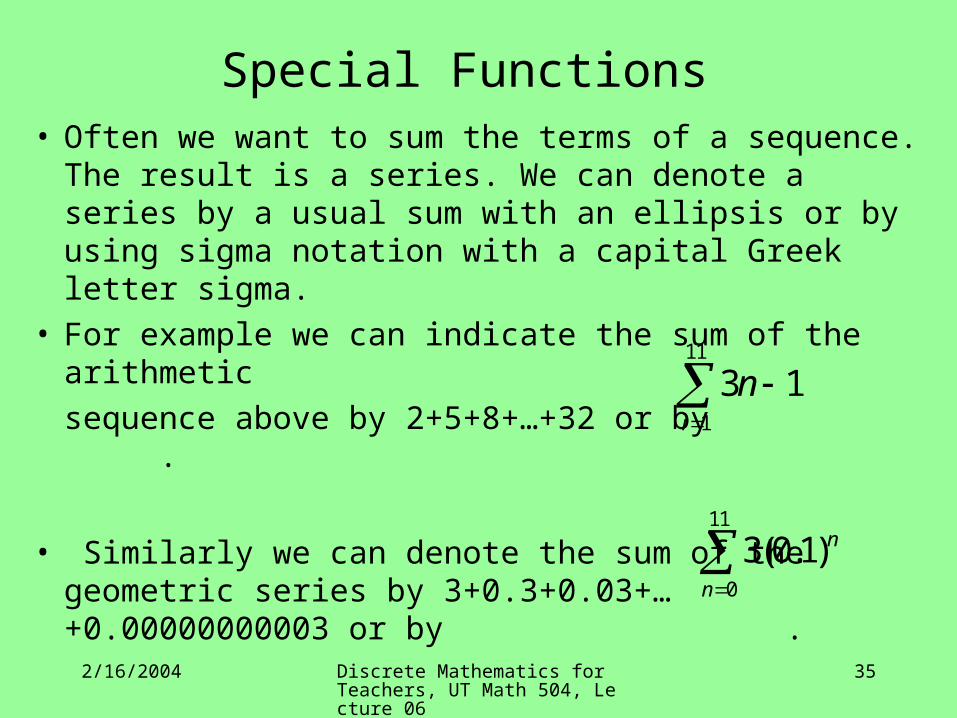
Special Functions • Often we want to sum the terms of a sequence. The

result is a series. We can denote a series by a usual sum with an ellipsis or by using sigma notation with a capital Greek letter sigma.

• For example we can indicate the sum of the arithmetic

sequence above by 2+5+8+…+32 or by .

• Similarly we can denote the sum of the geometric series by 3+0.3+0.03+…+0.00000000003 or by .

11

1

3 1i

n

11

0

3(0.1)n

n


36

Special Functions• Since the successive terms of an arithmetic sequence

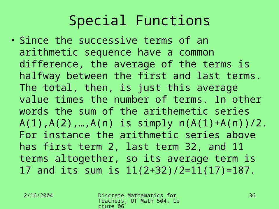
have a common difference, the average of the terms is halfway between the first and last terms. The total, then, is just this average value times the number of terms. In other words the sum of the arithemetic series A(1),A(2),…,A(n) is simply n(A(1)+A(n))/2. For instance the arithmetic series above has first term 2, last term 32, and 11 terms altogether, so its average term is 17 and its sum is 11(2+32)/2=11(17)=187.


37

Special Functions

• The formula for summing a geometric series is a little more subtle, but the argument that proves it is well worth understanding (it comes up in many other mathematical contexts). The book presents it just after example 4.14 on p. 145.


38

Matrices

• Matrices as functions: We usually think of matrices as rectangular arrays of numbers. For instance an m×n matrix of real numbers contains mn real numbers, each of which is identified by the row and column in which it is located. This effectively defines a function from the set of positions (i,j) into the real numbers. That is, if A is the name of the matrix, then A:{1,2,…,m}×{1,2,…,n}→ℝ. To denote to the entry in row i and column j we could use A(i,j), but it is more common to use Aij or aij. We

can then describe the matrix as A=[ Aij] or A=[ aij].


39

Matrices

• Rectangular representation: At the top of p. 147 the book illustrates how to display a general matrix as a rectangular array. The dimensions of a matrix with m rows and n columns (i.e., a function with domain :{1,2,…,m}×{1,2,…,n }) is m×n.

• Element/entry/component. The individual numbers in the matrix (the elements of the codomain) are called elements, entries, or components of the matrix.


40

Matrices

• Row/Column/Square matrices: A 1×n matrix is a row matrix. An n×1 matrix is a column matrix. An n×n matrix is a square matrix.

• Equality of matrices: Matrices are equal if they have the same entries in the same locations. Equivalently, they are equal if they are equal as functions.


41

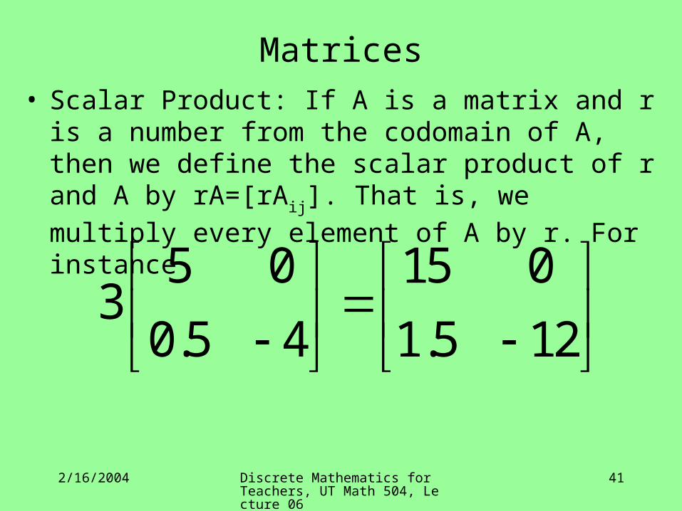
Matrices• Scalar Product: If A is a matrix and r is a number from

the codomain of A, then we define the scalar product of r and A by rA=[rAij]. That is, we multiply every element

of A by r. For instance

5 0 15 03

0.5 4 1.5 12


42

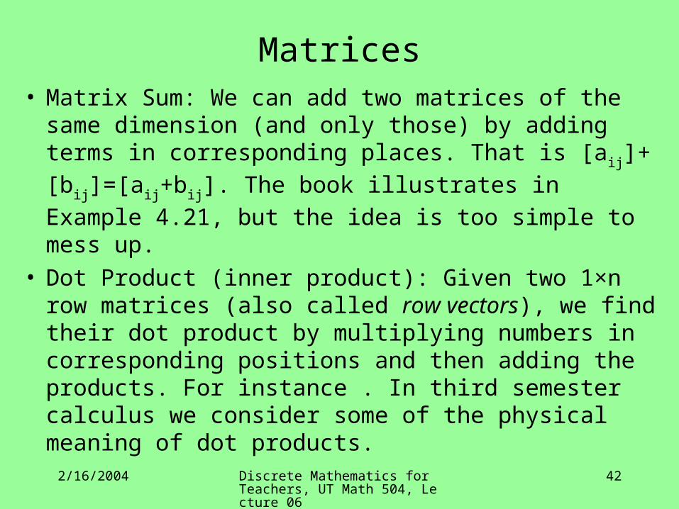
Matrices• Matrix Sum: We can add two matrices of the same

dimension (and only those) by adding terms in corresponding places. That is [aij]+[bij]=[aij+bij]. The

book illustrates in Example 4.21, but the idea is too simple to mess up.

• Dot Product (inner product): Given two 1×n row matrices (also called row vectors), we find their dot product by multiplying numbers in corresponding positions and then adding the products. For instance . In third semester calculus we consider some of the physical meaning of dot products.


43

Matrices• Matrix Product: If matrix A is m×n and matrix B is n×p,

then we can define the matrix product AB to be the m×p matrix [cij], where cij is the dot product of the ith row of A

with the jth column of B. Again the book gives a good example of this procedure in example 4.23 on page 149. Although it is not obvious why such a bizarre operation would be useful, this definition of matrix multiplication turns out to have a natural interpretation in many contexts.

• Transpose: If A=[aij] is an m×n matrix, then the

transpose of A is the n×m matrix At=[aji].


44

Matrices• The book gives several theorems about matrix

arithmetic, all of which depend on the properties of real arithmetic and perhaps careful consideration of the summations involved in matrix multiplication. They establish that matrix addition is commutative and associative, that matrix multiplication is associative, and that matrix multiplication distributes over addition. Also scalar products cooperate with other operations in an intuitively reasonable fashion. Note however that matrix multiplication is not commutative, even when the matrices involved are square.


45

Matrices• The transpose of the product equals product of the

transposes in the opposite order (4.29). Proof: This is just a matter of careful bookkeeping.


46

Matrices• Symmetric: A matrix is symmetric if it equals its own

transpose. Unavoidably this requires the matrix be square. Intuitively it means that the upper right and lower left halves of the matrix are mirror images of each other with the mirror lying on the diagonal of the matrix. (The diagonal always means the diagonal from upper left to lower right).


47

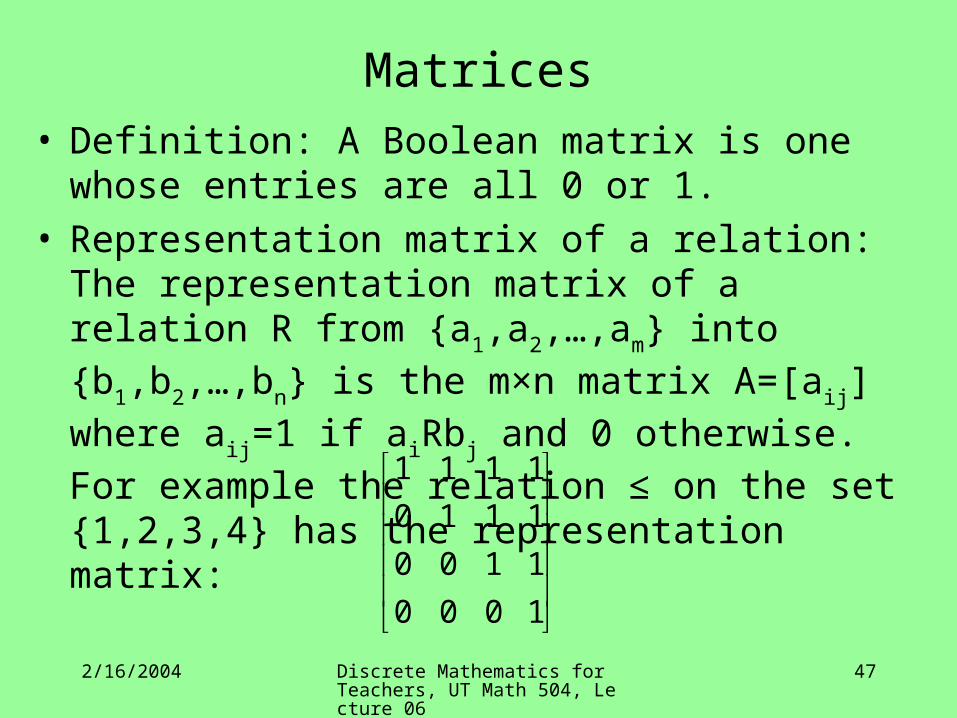
Matrices• Definition: A Boolean matrix is one whose entries are all

0 or 1.• Representation matrix of a relation: The representation

matrix of a relation R from {a1,a2,…,am} into {b1,b2,

…,bn} is the m×n matrix A=[aij] where aij=1 if aiRbj and

0 otherwise. For example the relation ≤ on the set {1,2,3,4} has the representation matrix:

1 1 1 1

0 1 1 1

0 0 1 1

0 0 0 1


48

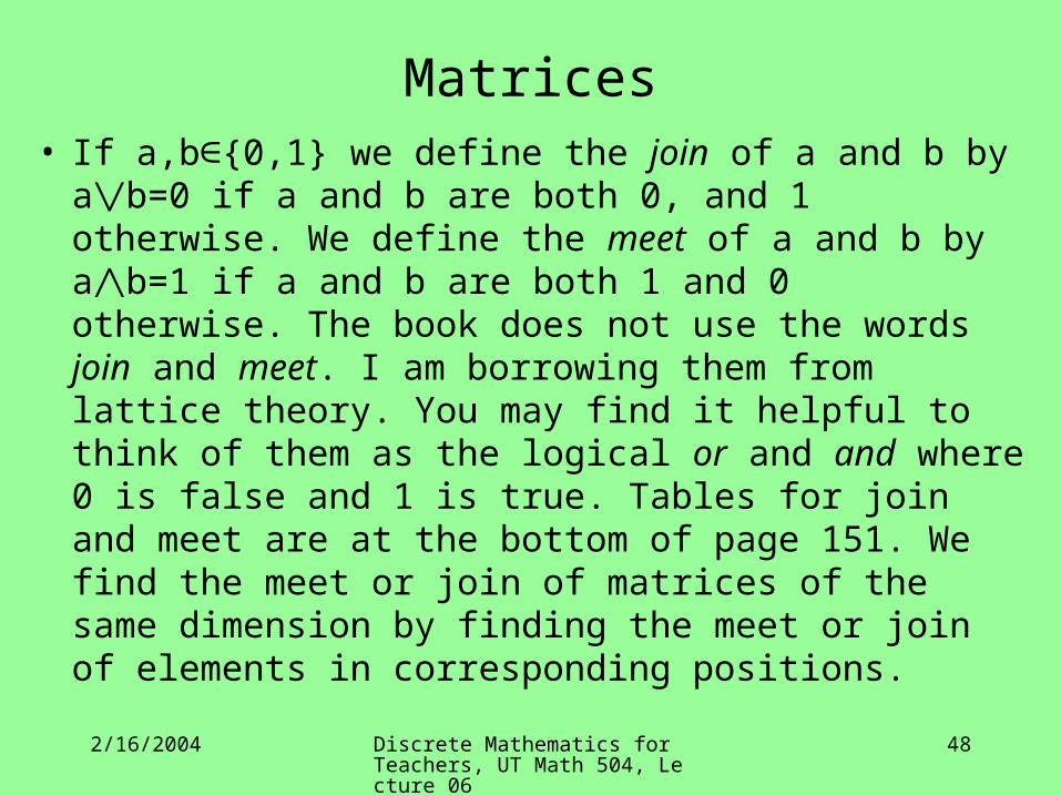
Matrices• If a,b∈{0,1} we define the join of a and b by a⋁b=0 if a

and b are both 0, and 1 otherwise. We define the meet of a and b by a⋀b=1 if a and b are both 1 and 0 otherwise. The book does not use the words join and meet. I am borrowing them from lattice theory. You may find it helpful to think of them as the logical or and and where 0 is false and 1 is true. Tables for join and meet are at the bottom of page 151. We find the meet or join of matrices of the same dimension by finding the meet or join of elements in corresponding positions.


49

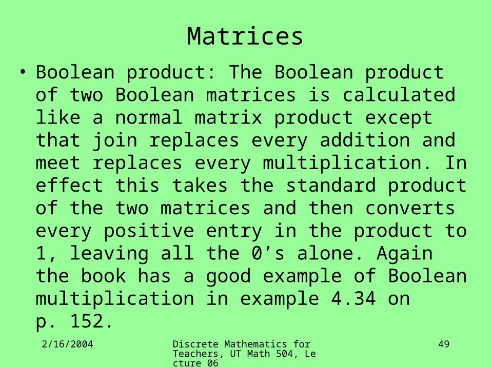
Matrices• Boolean product: The Boolean product of two Boolean

matrices is calculated like a normal matrix product except that join replaces every addition and meet replaces every multiplication. In effect this takes the standard product of the two matrices and then converts every positive entry in the product to 1, leaving all the 0’s alone. Again the book has a good example of Boolean multiplication in example 4.34 on p. 152.


50

Matrices• Characterization of representation matrices for reflexive,

symmetric, and transitive relations (4.35abc): The representation matrix of a relation on a set has 1’s on the diagonal if the relation is reflexive. It is symmetric (as a matrix) if the relation is symmetric (as a relation). It is transitive if its “Boolean square” has no 1’s in positions in which the original representation matrix has 0’s.


51

Matrices• Characterization of representation matrices for the union

and intersection of relations (4.35de). The representation matrix for the union of two relations is the join of their individual representation matrices. Similarly the intersection of the relations is represented by the meet of the matrices.


52

Matrices

• Characterization of representation matrices for the composition of relations (4.36): The representation matrix for the composition of two relations is given by the Boolean product of the two individual representation matrices (the order is important because of noncommutativity — see theorem 4.36 and the following example for details).


53

Matrices• Characterization of representation matrices for reflexive,

symmetric, and transitive relations (4.38): Let A be the representation matrix for a relation R. Then the representation matrix for the reflexive closure of R is simply A joined with the identity matrix of the same dimensions. The representation matrix for the symmetric closure of R is simply A joined to its transpose. The representation matrix for the symmetric closure of R is A joined to all of its Boolean powers up the the nth.


54

Matrices

• Definition: A permutation matrix is a square Boolean matrix with exactly one 1 in each row and column. If it were a chessboard and the 1’s were rooks, the rooks would cover every square but no rook would attack another.


55

Matrices• Theorem explaining the name (4.40). If M is an n×n

permutation matrix and A is an n×1 column matrix, then MA is a permutation of the entries in A. Namely, if M has a 1 in the ith row, jth column, then the jth entry in A appears in the ith entry in MA.

Documents

Number Theory, Special Functions, Matrices. 2/16/2004Discrete Mathematics for Teachers, UT Math 504, Lecture 06 2 Number Theory Basic Notation and Terms: