Embed Size (px)
Citation preview

NumCosmo – Overview and examples
Sandro D. P. Vitenti1,2
Mariana Penna-Lima1,3
Cyrille Doux3
1CBPF - Centro Brasileiro de Pesquisas Fısicas
2 UEL - Universidade Estadual de Londrina
3AstroParticule et Cosmologie (APC) – Universite Paris Diderot
XIII Workshop on New Physics in Space - Sao Paulo – November 30,2016
Sandro D. P. Vitenti1,2 Mariana Penna-Lima1,3 Cyrille Doux3 NumCosmo – Overview and examples 1/29

NumCosmo – http://ascl.net/1408.013
Free software C library (GPL license);
Main goals:
Calculate multiple cosmological observables efficiently.Provide a set of tools to perform: cosmological (astrophysical)calculations (multiple probes) and data analyses.Collaborative tool: each object is developed separately,communicating through predefined interfaces.
GObject: object-oriented programming in C, reference basedgarbage collection, inheritance, etc.
GObjectIntrospection: automatic bindings between C, Python,Perl, Java, and others.
Serialization framework: saving/loading, sending throughnetwork.
Sandro D. P. Vitenti1,2 Mariana Penna-Lima1,3 Cyrille Doux3 NumCosmo – Overview and examples 2/29

NumCosmo
Basic concepts
Ncm prefix – stands for NumCosmoMath which contains thegeneral codes not specific to cosmology, e.g., NcmSpline2d,ncm sf sbessel.
Nc prefix – represents the cosmological codes written on topof Ncm.
NcmModel – is a GObject and an abstract class whichbasically defines a set of parameters.
NcmMSet – is a collection of models which can containmodels of the same and/or different families.
NcmData – is an abstract class which encapsulates functionssuch as resample, −2 ln L, bootstrap resample...
NcmDataSet – is a collection of NcmData (combined probes).
Sandro D. P. Vitenti1,2 Mariana Penna-Lima1,3 Cyrille Doux3 NumCosmo – Overview and examples 3/29

Example 1: Type Ia Supernova – Update all
NcmFit
NcmFitMCMC
NcmMSet
Model SetNcmLikelihood
NcmModel:pkey=0
NcHICosmo
NcHICosmoDE
NcHICosmoDEXcdm
NcmModel:pkey=0
NcSNIADistCov
NcDistance
NcmDataSet
NcmDataGaussCov
NcDataSNIACov
−2 ln(LSNIa) = ∆ ~mTC−1SNIa(α, β)∆ ~m,
∆mi = mBi−5 log10(DL(zheli , zcmb
i ))+αXi−βCi−Mhi +5 log10(c/H0)−25,
α and β are related to the stretch-luminosity and colour-luminosity,respectively, and Mhi are absolute magnitudes.
Sandro D. P. Vitenti1,2 Mariana Penna-Lima1,3 Cyrille Doux3 NumCosmo – Overview and examples 4/29

Example 1: Type Ia Supernova – Update all
NcmFit
NcmFitMCMC
NcmMSet
Model SetNcmLikelihood
NcmModel:pkey=1
NcHICosmo
NcHICosmoDE
NcHICosmoDEXcdm
NcmModel:pkey=1
NcSNIADistCov
NcDistance
NcmDataSet
NcmDataGaussCov
NcDataSNIACov
−2 ln(LSNIa) = ∆ ~mTC−1SNIa(α, β)∆ ~m,
∆mi = mBi−5 log10(DL(zheli , zcmb
i ))+αXi−βCi−Mhi +5 log10(c/H0)−25,
α and β are related to the stretch-luminosity and colour-luminosity,respectively, and Mhi are absolute magnitudes.
Sandro D. P. Vitenti1,2 Mariana Penna-Lima1,3 Cyrille Doux3 NumCosmo – Overview and examples 4/29

Example 2: Type Ia Supernova – Update cosmo only
NcmFit
NcmFitMCMC
NcmMSet
Model SetNcmLikelihood
NcmModel:pkey=0
NcHICosmo
NcHICosmoDE
NcHICosmoDEXcdm
NcmModel:pkey=0
NcSNIADistCov
NcDistance
NcmDataSet
NcmDataGaussCov
NcDataSNIACov
−2 ln(LSNIa) = ∆ ~mTC−1SNIa(α, β)∆ ~m,
∆mi = mBi−5 log10(DL(zheli , zcmb
i ))+αXi−βCi−Mhi +5 log10(c/H0)−25,
Sandro D. P. Vitenti1,2 Mariana Penna-Lima1,3 Cyrille Doux3 NumCosmo – Overview and examples 5/29

Example 2: Type Ia Supernova – Update cosmo only
NcmFit
NcmFitMCMC
NcmMSet
Model SetNcmLikelihood
NcmModel:pkey=1
NcHICosmo
NcHICosmoDE
NcHICosmoDEXcdm
NcmModel:pkey=0
NcSNIADistCov
NcDistance
NcmDataSet
NcmDataGaussCov
NcDataSNIACov
−2 ln(LSNIa) = ∆ ~mTC−1SNIa(α, β)∆ ~m,
∆mi = mBi−5 log10(DL(zheli , zcmb
i ))+αXi−βCi−Mhi +5 log10(c/H0)−25,
Sandro D. P. Vitenti1,2 Mariana Penna-Lima1,3 Cyrille Doux3 NumCosmo – Overview and examples 5/29

Example 3: CMB TT only
NcmFit
NcmFitMCMC
NcmMSet
Model SetNcmLikelihood
NcmModel:pkey=0
NcHIPrim
NcHIPrimPowerLaw
NcmModel:pkey=0
NcHIReion
NcHIReionCAMB
NcmModel:pkey=0
NcHICosmo
NcHICosmoDE
NcHICosmoDEXcdm
NcmModel:pkey=0
NcPlanckFI
NcPlanckFICorTT
NcHIPertBoltzmann
NcHIPertBoltzmannCBE
NcmDataSet
NcDataPlanckLKL
NcHIPrimPowerLaw: simple power law for the primordialpower spectrum.
NcHIReionCAMB: CAMB’s reionization scheme.
NcPlanckFICorTT: Planck foreground and instrumentsparameters.
Sandro D. P. Vitenti1,2 Mariana Penna-Lima1,3 Cyrille Doux3 NumCosmo – Overview and examples 6/29

Software Quality Assurance
Unit testing: Test file for each object to assure the correctbehavior of each part of NumCosmo.
NcmC (fundamental physical and mathematical constants):CODATA (2014), IAU (2015), NIST
NcmSplineFunc – Automatic determination of the splineknots, given a precision.
Autotools – Widely used build-system, support severaloperational systems and architectures, compilers, easilyintegrated with Linux distributions and MacPorts.Not reinventing the wheel – Uses well known and testedlibraries as back-end:
GLib (object system/portability);Cuba (multidimensional integration);NLopt (non-linear optimization);GSL (several scientific algorithms);cfitsio (fits file manipulation);Sundials (ODE integrator);
Sandro D. P. Vitenti1,2 Mariana Penna-Lima1,3 Cyrille Doux3 NumCosmo – Overview and examples 7/29

CMB status:
CLASS and the Planck’s likelihood (clik) are integrated in thelibrary building system.
Abstract Planck foreground and instrument models are defined byNcPlanckFI, NcPlanckFICorTT and NcPlanckFICorTTTEEE.
CLASS interface is described in the CLASS Backend object NcCBE.
Interface to Cl through NcHIPertBoltzmann and Planck’s likelihoodthrough NcDataPlanckLKL.
Currently fully working implementation of NcHIPertBoltzmann:CLASS based NcHIPertBoltzmannCBE.
Standard NumCosmo implementation NcHIPertBoltzmannStd, workin progress, support for seeds and GI implementation.
Sandro D. P. Vitenti1,2 Mariana Penna-Lima1,3 Cyrille Doux3 NumCosmo – Overview and examples 8/29

CMB status:
Alternative primordial power spectra interface:
NcHIPrimAtan: implements an inverse tangent modification ofthe power spectrum.NcHIPrimExpc: implements exponential cutoff powerspectrum.NcHIPrimBPL: implements broken power law power spectrum.
Thermodynamics through CLASS NcRecombCBE,NumCosmo implementation NcRecombSeager (provides asingle pass integration for the whole system, same equationsas RECFAST).
Linear matter power spectrum NcPowspecML, interface toCLASS Matter Transfer Function NcPowspecMLCBE
Matter power spectrum non-linear correctionsNcPowspecMNL through Halofit NcPowspecMNLHalofit(Halo model in the next release).
Sandro D. P. Vitenti1,2 Mariana Penna-Lima1,3 Cyrille Doux3 NumCosmo – Overview and examples 9/29

Observational Probes
1 SNeIa: NcDataSNIACov:NcmDataGaussCov(NcDataDistMu:NcmDataGaussDiag for diagonal errors)
2 Galaxy Cluster: NcDataClusterNCount:NcmData,NcDataClusterPoisson:NcmDataPoisson,NcDataClusterPseudoCounts:NcmData
3 BAO: NcDataBaoRDV:NcmDataGaussDiag,NcDataBaoEmpiricalFit:NcmDataDist1d . . .
4 H(z): NcDataHubble:NcmDataGaussDiag
5 CMB distance priors: NcDataCMBDistPriors:NcmDataGauss
6 CMB: NcDataPlanckLKL:NcmData7 Cross-Correlation: NcDataXcor:NcmDataGaussCov
Galaxies, QSO: NcXcorLimberGal:NcXcorLimberCMB lensing: NcXcorLimberLensing:NcXcorLimber
Sandro D. P. Vitenti1,2 Mariana Penna-Lima1,3 Cyrille Doux3 NumCosmo – Overview and examples 10/29

Matter power spectrum products
NcPowspecMLCBE: CLASS linear matter power spectrum;NcPowspecMLTransfer + NcTransferFuncEH +NcGrowthFunc: Eisenstein and Hu (EH);
10-5 10-4 10-3 10-2 10-1 100 101 102
k [Mpc−1]
10-15
10-13
10-11
10-9
10-7
10-5
10-3
10-1
101
k 3P(k, z)/(2π2)
CLASS z= 0. 00
EH z= 0. 00
CLASS z= 1. 00
EH z= 1. 00
CLASS z= 2. 00
EH z= 2. 00
Sandro D. P. Vitenti1,2 Mariana Penna-Lima1,3 Cyrille Doux3 NumCosmo – Overview and examples 11/29

Matter power spectrum products
CLASS vs EH linear matter power spectrum;
10-5 10-4 10-3 10-2 10-1 100 101 102
k [Mpc−1]
10-8
10-7
10-6
10-5
10-4
10-3
10-2
10-1 |1−PEH(k, z)/PCLASS(k, z)|
CLASS EH cmp z= 0. 00
CLASS EH cmp z= 0. 50
CLASS EH cmp z= 1. 00
CLASS EH cmp z= 1. 50
CLASS EH cmp z= 2. 00
Sandro D. P. Vitenti1,2 Mariana Penna-Lima1,3 Cyrille Doux3 NumCosmo – Overview and examples 12/29

Matter power spectrum products
CLASS + NcPowspecMNLHaloFit;
10-5 10-4 10-3 10-2 10-1 100 101 102
k [Mpc−1]
10-15
10-13
10-11
10-9
10-7
10-5
10-3
10-1
101
103
105
k 3P(k, z)/(2π2)
CLASS z= 0. 00
CLASS+HaloFit z= 0. 00
CLASS z= 5. 00
CLASS+HaloFit z= 5. 00
CLASS z= 10. 00
CLASS+HaloFit z= 10. 00
Sandro D. P. Vitenti1,2 Mariana Penna-Lima1,3 Cyrille Doux3 NumCosmo – Overview and examples 13/29

Matter power spectrum products
NcmPowspecFilter + CLASS: σ8 = 0.846;NcmPowspecFilter + EH: σ8 = 0.853;NcmPowspecFilter uses NcmFftlog to compute∫∞
0 jl(kR)2P(k , z)k2dk efficiently.
10-4 10-3 10-2 10-1 100 101 102 103 104 105
R [Mpc]
10-7
10-6
10-5
10-4
10-3
10-2
10-1
100
101
102 Tophat filtered σ(R)
σ CLASS z= 0. 00
σ EH z= 0. 00
σ CLASS z= 1. 00
σ EH z= 1. 00
σ CLASS z= 2. 00
σ EH z= 2. 00
Sandro D. P. Vitenti1,2 Mariana Penna-Lima1,3 Cyrille Doux3 NumCosmo – Overview and examples 14/29
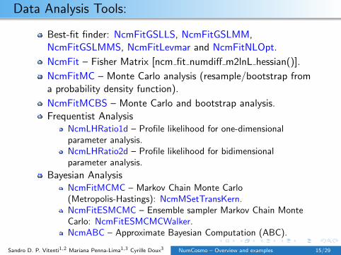
Data Analysis Tools:
Best-fit finder: NcmFitGSLLS, NcmFitGSLMM,NcmFitGSLMMS, NcmFitLevmar and NcmFitNLOpt.
NcmFit – Fisher Matrix [ncm fit numdiff m2lnL hessian()].
NcmFitMC – Monte Carlo analysis (resample/bootstrap froma probability density function).
NcmFitMCBS – Monte Carlo and bootstrap analysis.Frequentist Analysis
NcmLHRatio1d – Profile likelihood for one-dimensionalparameter analysis.NcmLHRatio2d – Profile likelihood for bidimensionalparameter analysis.
Bayesian AnalysisNcmFitMCMC – Markov Chain Monte Carlo(Metropolis-Hastings): NcmMSetTransKern.NcmFitESMCMC – Ensemble sampler Markov Chain MonteCarlo: NcmFitESMCMCWalker.NcmABC – Approximate Bayesian Computation (ABC).
Sandro D. P. Vitenti1,2 Mariana Penna-Lima1,3 Cyrille Doux3 NumCosmo – Overview and examples 15/29

ESMCMC example
gi.require_version(’NumCosmo’, ’1.0’)gi.require_version(’NumCosmoMath’, ’1.0’)
from gi.repository import NumCosmo as Ncfrom gi.repository import NumCosmoMath as Ncm
# Main library initializationNcm.cfg_init ()Ncm.func_eval_set_max_threads (40)
# New CLASS backend precision objectcbe_prec = Nc.CBEPrecision.new ()cbe = Nc.CBE.prec_new (cbe_prec)
# New Boltzmann CLASS backend objectbz_cbe = Nc.HIPertBoltzmannCBE.full_new (cbe)
# Loading MSet and setting Omega_k = 0.mset = Ncm.MSet.load ("model_set_file.mset", ser)cosmo = mset.peek (Nc.HICosmo.id ())
cosmo.param_set_by_name ("Omegak", 0.0)
Sandro D. P. Vitenti1,2 Mariana Penna-Lima1,3 Cyrille Doux3 NumCosmo – Overview and examples 16/29

ESMCMC example
# New Dataset objectdset = Ncm.Dataset.new ()
lkls = [’DataV2/commander_rc2_v1.1_l2_29_B.clik’,’DataV2/plik_dx11dr2_HM_v18_TT.clik’]
for lkl in lkls:plik = Nc.DataPlanckLKL.full_new (lkl, bz_cbe)dset.append_data (plik)
# Load SNIa data.fitsname = "jla_snls3_sdss_sys_stat_cmpl.fits"data_snia = Nc.DataSNIACov.new (False)data_snia.load (fitsname)
dset.append_data (data_snia)
# Creating a Likelihood from the Dataset.lh = Ncm.Likelihood (dataset = dset)Nc.PlanckFICorTT.add_all_default_priors (lh)
Sandro D. P. Vitenti1,2 Mariana Penna-Lima1,3 Cyrille Doux3 NumCosmo – Overview and examples 17/29

ESMCMC example
# Creating a Fit objectfit = Ncm.Fit.new (Ncm.FitType.NLOPT, algorithm,
lh, mset, Ncm.FitGradType.NUMDIFF_CENTRAL)
# Initial samplerinit_sampler = Ncm.MSetTransKernGauss.new (0)init_sampler.set_mset (mset)init_sampler.set_prior_from_mset ()init_sampler.set_cov_from_rescale (0.1)
# The ensemble sampler walker typenwalkers = 100stretch = Ncm.FitESMCMCWalkerStretch.new (nwalkers,
mset.fparams_len ())stretch.set_box_mset (mset)stretch.set_scale (1.2)
# ESMCMC objectesmcmc = Ncm.FitESMCMC.new (fit, nwalkers, init_sampler,
stretch, Ncm.FitRunMsgs.FULL)esmcmc.set_nthreads (40)
Sandro D. P. Vitenti1,2 Mariana Penna-Lima1,3 Cyrille Doux3 NumCosmo – Overview and examples 18/29

ESMCMC example
# Setting outputesmcmc.set_data_file ("output_chains.fits")
# Running ...esmcmc.start_run ()esmcmc.run_lre (1, 1.0e-3)esmcmc.end_run ()
esmcmc.mean_covar ()fit.log_covar ()
Sandro D. P. Vitenti1,2 Mariana Penna-Lima1,3 Cyrille Doux3 NumCosmo – Overview and examples 19/29

ESMCMC example
Snapshot of a ESMCMC run using Planck TT data and a modifiedprimordial power spectrum.
Object: NcmFitESMCMC,
Walker: NcmFitESMCMCWalkerStretch,
Output: a NcmMSetCatalog object serialized in a fits file.
# Elapsed time: 01 days, 21:57:54.8427910# degrees of freedom [002523]# m2lnL = 796.42768789029# Fit parameters:# 69.8108499055435 0.115986617072077 0.0226852361053738 3.23602243188527# NcmMSetCatalog: Current mean: 854.15 69.938 0.11588 0.022799# NcmMSetCatalog: Current msd: 0.54997 0.0049737 1.2071e-05 1.8152e-06# NcmMSetCatalog: Current sd: 511.73 0.90615 0.0020219 0.00036516# NcmMSetCatalog: Current var: 2.6187e+05 0.82111 4.0882e-06 1.3334e-07# NcmMSetCatalog: Current tau: 1 26.084 30.858 21.395# NcmMSetCatalog: Current skfac: 1.0029 1.1474 1.1388 1.0652# NcmMSetCatalog: Maximal Shrink factor = 1.25590891624521# NcmFitESMCMC:acceptance ratio 62.5521%, offboard ratio 0.0000%.# Task:NcmFitESMCMC, completed: 865800 of 10371900, elapsed time: 1 day, 21:57:54.8162# Task:NcmFitESMCMC, mean time: 00:00:00.1911 +/- 00:00:00.0036# Task:NcmFitESMCMC, time left: 21 days, 00:40:40.0570 +/- 09:22:42.2361# Task:NcmFitESMCMC, estimated to end at: Tue May 17 2016, 07:18:32 +/- 09:22:42.2361
Sandro D. P. Vitenti1,2 Mariana Penna-Lima1,3 Cyrille Doux3 NumCosmo – Overview and examples 20/29

Data Analysis Tools:
mcat analyze:
Compute 1− 3σconfidence intervals forthe best-fit, mean, modeor median of marginaldistributions.Compute covariancematrix.
de mc plot.py: make plot ofhistograms of marginalparameter distributions andthe bidimensional contours.
0.5 0.6 0.7 0.8 0.9 1.0 1.1αSZ
0.2
0.4
0.6
0.8
1−b SZ
0.6
83
0.9
55
0.99
3
de mc corner plot.py: makecorner plot.
0.4
0.6
0.8
1.0
1−b SZ
0.0
0.3
0.6
0.9
σSZ
0.0
0.2
0.4
0.6
σL
0.6
0.9
1.2
1.5
αSZ
0.6
0.0
0.6
r
0.4
0.6
0.8
1.0
1− bSZ
0.0
0.3
0.6
0.9
σSZ
0.0
0.2
0.4
0.6
σL
0.6
0.0
0.6
r
Sandro D. P. Vitenti1,2 Mariana Penna-Lima1,3 Cyrille Doux3 NumCosmo – Overview and examples 21/29

Example: Chains evolution
-12
-10
-8
-6
-4
-2
0
2
4
6
8
10
0 500 1000 1500 2000 2500
H0OcObAsnsc1c2c3zre
Sandro D. P. Vitenti1,2 Mariana Penna-Lima1,3 Cyrille Doux3 NumCosmo – Overview and examples 22/29
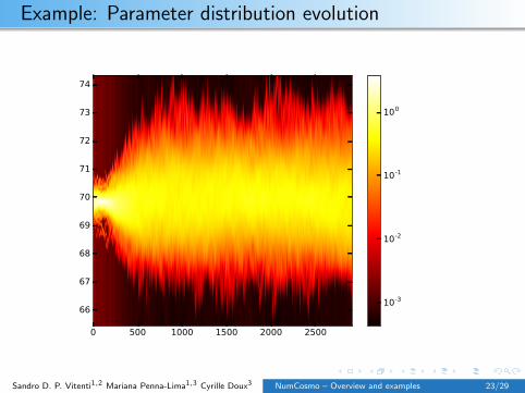
Example: Parameter distribution evolution
0 500 1000 1500 2000 2500
66
67
68
69
70
71
72
73
74
10-3
10-2
10-1
100
Sandro D. P. Vitenti1,2 Mariana Penna-Lima1,3 Cyrille Doux3 NumCosmo – Overview and examples 23/29

Conclusions
NumCosmo is a suitable framework for collaborations /collaborative work.Further NumCosmo objects can be directly implemented inPython or in any other bound language.github.com/NumCosmo/NumCosmowww.nongnu.org/numcosmo/
References :M. Penna-Lima et al. [JCAP05(2014)039], arXiv:1312.4430 – Cluster number counts, spline 2D, ProfileLikelikood, MC (resample), Fisher matrix.E. Ishida, S. Vitenti, M. Penna-Lima, et al. [Astronomy and Computing, Vol. 13 (2015) p. 1-11],arXiv:1504.06129 – Approximate Bayesian Computation.S. Vitenti and M. Penna-Lima [JCAP09(2015)045], arxiv:1505.01883 – SNeIa, BAO, H(z), spline 1D, MC,resample - bootstrap, ESMCMC.M. Penna-Lima, J. Bartlett, et al. (submitted to A&A): Cluster pseudo counts, ESMCMC.P. Peter, A. Valentini, S. Vitenti: Non-equilibrium primordial powerspectrum in prep. – NcHIPrimAtan,NcDataPlanckLKL, NcPlanckFICorTT, ESMCMC.S. Vitenti, MPL, C. Doux: NumCosmo in prep.C. Doux, MPL, S. Vitenti: NcXCor in prep.
Obrigado!
Sandro D. P. Vitenti1,2 Mariana Penna-Lima1,3 Cyrille Doux3 NumCosmo – Overview and examples 24/29

Conclusions
NumCosmo is a suitable framework for collaborations /collaborative work.Further NumCosmo objects can be directly implemented inPython or in any other bound language.github.com/NumCosmo/NumCosmowww.nongnu.org/numcosmo/
References :M. Penna-Lima et al. [JCAP05(2014)039], arXiv:1312.4430 – Cluster number counts, spline 2D, ProfileLikelikood, MC (resample), Fisher matrix.E. Ishida, S. Vitenti, M. Penna-Lima, et al. [Astronomy and Computing, Vol. 13 (2015) p. 1-11],arXiv:1504.06129 – Approximate Bayesian Computation.S. Vitenti and M. Penna-Lima [JCAP09(2015)045], arxiv:1505.01883 – SNeIa, BAO, H(z), spline 1D, MC,resample - bootstrap, ESMCMC.M. Penna-Lima, J. Bartlett, et al. (submitted to A&A): Cluster pseudo counts, ESMCMC.P. Peter, A. Valentini, S. Vitenti: Non-equilibrium primordial powerspectrum in prep. – NcHIPrimAtan,NcDataPlanckLKL, NcPlanckFICorTT, ESMCMC.S. Vitenti, MPL, C. Doux: NumCosmo in prep.C. Doux, MPL, S. Vitenti: NcXCor in prep.
Obrigado!Sandro D. P. Vitenti1,2 Mariana Penna-Lima1,3 Cyrille Doux3 NumCosmo – Overview and examples 24/29

COSMOMC + (CAMB or PICO)
.ini files
Program driven: one tool (mainly MCMC)Parameters: range, scale, fixed
Parameter priors: Gaussian onlyRun options: likelihoods, sampler, models
cosmomc
Creates Ini object from .ini filesBuild the likelihood using flags in Ini
Calls TCosmologyCalculator(CAMB Calculator or PICO Calculator)
CAMBPICO
Calculates the cosmological observ-able necessary for the likelihoods
cosmomcCalculates the next proposal points and calls
the Calculator to evaluate the likelihoodaccept/reject and repeat . . .
getdist analysis of the chains and post processing
many text files, emulatesa script language
Ini object holdsall definitions
All observables must bedefined in Ini matching
CAMB/PICO parameters
Creates text filescontaining the chains,
one for each chain
Reads from text files,separated from cos-
momc, cannot performcosmological calculations
Sandro D. P. Vitenti1,2 Mariana Penna-Lima1,3 Cyrille Doux3 NumCosmo – Overview and examples 25/29

NumCosmo
Scripts orprograms
Library driven: many toolsCreates/Loads: models, priors, data
Extensible: new priors, samplers, modelsAvoids flags: one script/program per task
NumCosmoNcmLikelihood
NcmMSet
Handles each object separatelyNew likelihoods without modifying sources
Can use different models and back-endsModels grouped together in NcmMSet
NumCosmoNcmDataset
NcmLikelihoodNcmFit?
Different analysis tools:NcmFit: best-fit and Fisher matrix
NcmLHRatio1/2d: frequentist confidence regionsNcmFitMC: MC resampling or bootstrapingNcmFitMCMC: MCMC NcmMSetTransKern
NcmFitESMCMC: Ensemble sam-pler MCMC NcmFitESMCMCWalker
NumCosmoNcmMSetCatalog
Handles the output of all samplersChains’ checkpoint
MCMC diagnostics: Shrink factor, au-tocorrelation time, visual diagnostics
mcat analyzeanalysis of the chains and post processing
can perform cosmological calcula-tions for each point in the chains
programming lan-guage, easier debugging
and error checking
All objects com-municate throughcommon interfaces
Independent tools,common output
Sync to a single fits(cfitsio) file containingall chains/checkpoints
Fast to read binaryfiles, part of NumCosmo
Sandro D. P. Vitenti1,2 Mariana Penna-Lima1,3 Cyrille Doux3 NumCosmo – Overview and examples 26/29

Theory vs Observations
Likelihood: Probability of measuring “Data” given a “Model”
L(Data|Model)
Alternatives: Approximated Bayesian computation, simulations
Theory (Models)
Modeling observablesModeling uncertainties
Observations (Data)
Data pointsUncertainties
Probability Distribution (Statistics)
Hypothesis about the uncertainties ⇒ Likelihood form (Bayesiananalysis, posterior, priors)
Data Analysis
Methodology to extract information from the Data: parameterconstraints, model testing, model comparison, posterior exploration
Sandro D. P. Vitenti1,2 Mariana Penna-Lima1,3 Cyrille Doux3 NumCosmo – Overview and examples 27/29

Cross-correlations with NumCosmo I
For all observables that are linear functionals of the density field
a(θ) =
∫dzW (z)δ
(θχ(z), z
)(1)
Cross-spectra in the Limber approximation
C ab` =
∫ z∗
0dz
H(z)
c
1
χ(z)2∆a`(z)∆b
` (z)P
(k =
l + 1/2
χ(z), z
)(2)
with kernels
∆κ` (z) =
3Ωm
2
H20
H(z)(1 + z)χ(z)
χ∗ − χ(z)
χ∗(3)
∆g` (z) = b(z)
dn
dz+
3Ωm
2
H20
H(z)(1 + z)χ(z)
∫ z∗
zdz ′(
1−χ(z)
χ(z ′)
)(α(z ′)− 1
) dndz
(z ′)
(4)
Valid for CMB lensing, SZ, CIB, ISW, galaxy lensing, galaxydensity...
Sandro D. P. Vitenti1,2 Mariana Penna-Lima1,3 Cyrille Doux3 NumCosmo – Overview and examples 28/29
Cross-correlations with NumCosmo III
Goal is to extract as much information as available : use bothcross- AND auto-spectra Cκκ` , C gg
` , Cκg`Gaussian likelihood ready for correlation of n observables withpseudo-spectra
Constraints on biases + cosmological parameters
Statistical tools already available in NumCosmo and pluggable: MCMC, bootstrap, ABC, etc. !
Stable version available on GitHub
NumCosmo paper : Vitenti et al. in prep.
xcor paper : Doux et al. in prep.
Sandro D. P. Vitenti1,2 Mariana Penna-Lima1,3 Cyrille Doux3 NumCosmo – Overview and examples 29/29