Numerical and Experimental Determination of Nonlinear ...sd.engr.wisc.edu/.../10/Ehrhardt-Harris-Allen-NLCumminsPlate-IMAC20… · Ehrhardt, Harris & Allen - IMAC, Feb. 2014 Page

Ehrhardt, Harris & Allen - IMAC, Feb. 2014 Page 1 of 14

Numerical and Experimental Determination of Nonlinear Normal Modes of a Circular Perforated Plate

David A. Ehrhardt

Graduate Research Assistant

Ryan B. Harris Graduate Research Assistant

Matthew S. Allen1 Associate Professor

Department of Engineering Physics, University of Wisconsin-Madison, 535 Engineering Research Building, 1500 Engineering Drive, Madison, WI 53706

Abstract

It is commonly known that nonlinearities in structures can lead to large amplitude responses that are not predicted by traditional theories. Thus a linear design could lead to premature failure if the structure actually behaves nonlinearly, or, conversely, nonlinearities could potentially be exploited to reduce stresses relative to the best possible design with a purely linear structure. When examining structures that operate in environments where a nonlinear response is possible, one can gain insight into the free and force responses of a nonlinear system by determining the structure’s nonlinear normal modes (NNMs). NNMs extend knowledge gained from established linear normal modes (LNMs) into the nonlinear response range by quantifying how the unforced vibration frequency depends on the input energy. Recent works have shown that periodic excitations can be used to isolate a single NNM, providing a means for measuring NNMs in the laboratory. An extension of the modal indicator function can be used to ensure that the measured response is on the desired NNM. The experimentally measured NNMs can then be compared to numerically calculated NNMs for model validation. In this investigation, a circular perforated plate containing a distributed geometric nonlinearity is considered. This plate has demonstrated nonlinear responses when the displacements become comparable to the plate thickness. However, the system is challenging to model because the nonlinear response is potentially sensitive to small geometric features, residual stresses within the structure, and the boundary conditions.

1. Introduction

Structures have been shown to exhibit nonlinear responses when large deformations occur due to extreme mechanical and environmental loading conditions, or in other cases at seemingly small amplitudes if the structure contains materials with nonlinear constitutive properties or when thin shell geometries experience vibration levels approaching the shell thickness. Over the past several decades a suite of testing and modeling approaches has been developed for linear systems. The term linear is important here since characterization of systems using modal analysis is based on quantifying the system in terms of invariants such as resonant frequencies, damping rations, mode shapes, and frequency-response functions. Once these system invariants are quantified, a system model, typically a finite element model, is updated to reflect the measured properties. These techniques can not be directly applied to nonlinear systems since the linear system invariants become functions of input energy, so new methods are sought to address nonlinear behavior while preserving as much as possible the simplicity of the traditional design and test paradigms.

This work proposes to use the nonlinear normal mode (NNM) concept as a basis for testing and model updating of nonlinear structures. A structure’s nonlinear modes provide significant insight into the

1 Corresponding Author: [email protected]


structure’s free and forced response and they allow its behavior to be expressed in terms of a few compact plots [1]. For example, in a companion paper the authors explore how nonlinear modes can be used to evaluate the fidelity of a reduced order model [2], illustrating that when a structure’s NNMs are correctly modeled the model will be accurate for a range of different types of inputs, excitation levels, etc… Several advances in recent years have begun to make nonlinear modeling and testing for model updating a reality for realistic structures. First, new methods have been developed to calculate the nonlinear normal modes of a structure. Peeters et al. [3] recently presented a technique based on numerical integration and continuation which has proven effective for computing the NNMs of a structure with hundreds of degrees of freedom so long as the nonlinearities are localized. Allen, Kuether & Deaner [4, 5] recently extended that approach to structures with geometric nonlinearities that are modeled within commercial finite element software, making high fidelity model updating a possibility. On the testing front various approaches have been explored and one of the more promising seems to be a variant on stepped sine testing in which a structure can be made to vibrate in only one nonlinear mode [6]. The excitation can then be removed and the response would then presumably decay along that NNM. Peeters et al [7] applied this technique to a beam with a local nonlinearity at one end with good results. Kuether & Allen proposed a variant on this technique that was used to compute NNMs [8] but also could be extended to compute an NNM by progressively adjusting the excitation frequency and amplitude while observing an extension of the modal indicator function (MIF).

This work proceeds along similar lines, using stepped-sine testing to estimate the nonlinear frequency response of a structure over a range of excitation amplitudes and the NNMs are then estimated from the backbones of these nonlinear frequency responses. The methods developed in [4, 5] are then used to compute the NNMs of the geometrically nonlinear structure using a detailed finite element model, and then the experimentally estimated nonlinear modes are compared with those computed from the model to determine how the model should be updated. A simplified analytical model of the plate was also used in the initial troubleshooting, based on the work of Leissa [9], which details the analysis of the vibration of plates with various boundary conditions, thicknesses, and geometries using continuum vibrations. In reference to circular plates, Leissa uses Kirchhoff-Love plate theory to derive the various mode shapes and natural frequencies based on the geometry and boundary conditions. Additionally, we exploit the work of Jhung and Jo [10], who showed how one can precisely model a perforated plate by simply adjusting the elastic modulus and density based on the perforation geometry and pattern. This initial investigation focuses on the first two symmetric modes of the plate. The following section provides some background information regarding nonlinear normal modes while Section 2 discusses the testing that was performed. Section 3 describes the comparisons that were used to update the computational model and the results.

2. Analysis and Experimental Setup

2.1 Test Specimen

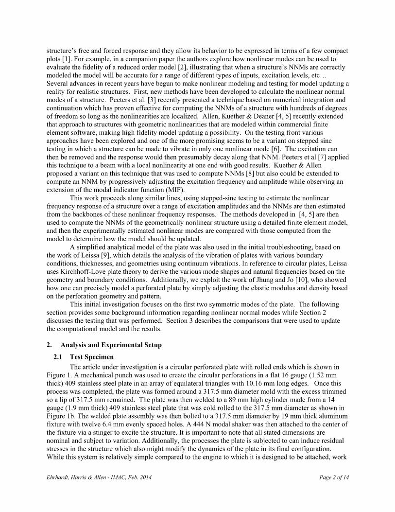
The article under investigation is a circular perforated plate with rolled ends which is shown in Figure 1. A mechanical punch was used to create the circular perforations in a flat 16 gauge (1.52 mm thick) 409 stainless steel plate in an array of equilateral triangles with 10.16 mm long edges. Once this process was completed, the plate was formed around a 317.5 mm diameter mold with the excess trimmed so a lip of 317.5 mm remained. The plate was then welded to a 89 mm high cylinder made from a 14 gauge (1.9 mm thick) 409 stainless steel plate that was cold rolled to the 317.5 mm diameter as shown in Figure 1b. The welded plate assembly was then bolted to a 317.5 mm diameter by 19 mm thick aluminum fixture with twelve 6.4 mm evenly spaced holes. A 444 N modal shaker was then attached to the center of the fixture via a stinger to excite the structure. It is important to note that all stated dimensions are nominal and subject to variation. Additionally, the processes the plate is subjected to can induce residual stresses in the structure which also might modify the dynamics of the plate in its final configuration. While this system is relatively simple compared to the engine to which it is designed to be attached, work


will show how important it is to have a test to validate any computational models that are created; there are a variety of subtle details that might easily be neglected initially, and yet they could change the response considerably.

(a)

(b)

(c)

Figure 1: Perforated Plate. a) perforated plate before welding into test configuration, b) Perforated plate welded into the supporting cylinder, c) based plate to which the system was

attached for testing.

2.2 Finite Element Model

Circular plates exhibit complex behavior which can be difficult to model, even in a linear range. In this investigation, a finite element model (FEM) was built based on the previously stated nominal geometries of the perforated plate before it was welded to the steel cylinder. Therefore, it is assumed that the welded boundary between the plate and steel cylinder provide fixed boundary conditions in the model. The plate curves from the weld and is flat over the entire central region, and hence will be referred to as a model with “No Initial Curvature (NIC)” in all of the following. A very fine mesh would have been required in order to model each of the perforations. However, Jhung and Jo [10] found that a perforated plate behaves identically to a non-perforated plate of the same dimensions, as long as the elastic


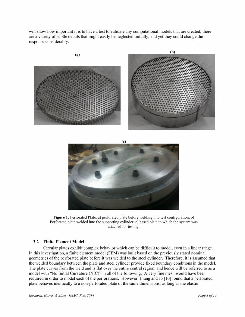
properties are adjusted appropriately. Hence, the reduced elastic modulus and density were calculated based on the perforation geometry as detailed by Jhung and Jo [10], which for the triangular perforation pattern of this plate yields a new elastic modulus of 1.68 GPa and density of 5120 kg/m3. The resulting meshed Abaqus model is shown in Figure 2, and has 1440 S4R shell elements. The elastic modulus was later updated based upon comparison with experiments. The reduced density was not updated because it can be computed from the geometric properties of the perforations (ex. size of hole and count) and hence it was thought to be quite accurate. On the other hand, the effective modulus is dependent on any residual stresses from the addition of perforations, or imperfections of the perforation location geometry.

Figure 2: Meshed Perforated Plate Model

The nonlinear normal modes of the plate were computed from this model using the procedure discussed in [4, 5]. Specifically, a reduced order model was created for each mode of the plate (separately) using the Implicit Condensation method [11-13]. Then the ROM was integrated in the NNMCont Matlab routine provided by Peeters, Kerschen, et al. [6] to compute the nonlinear modes. In [4, 5] this approach was found to provide an excellent approximation for the backbone of each NNM of a geometrically nonlinear beam while neglecting any internal resonances which would increase the computational cost.

2.3 Experimental Setup

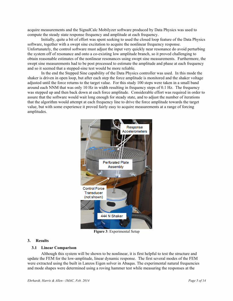
The experimental setup is shown in Figure 3. The 12.5 in circular perforated plate assembly previously described was attached to a Ling Dynamics LMT-100 electrodynamic shaker via a 5 mm diameter stinger. In some of the tests the shaker was controlled using closed loop feedback based on the input force measured by a Piezotronics PCB208C04 force transducer, with a sensitivity of 22 mV/N, mounted between the base plate and the stinger. The response of the plate is measured using two ISOTRON 25B accelerometers with a nominal sensitivity of 5 mV/g. The accelerometers were placed at two key points on the plate to ensure the dynamic response could be measured at the modes of interest. The first accelerometer, with a sensitivity of 4.627 mV/g; was placed in the center of the plate to identify modes that contain nodal diameters (ex. Mode 1, Mode 4, etc.). The second accelerometer, with a sensitivity of 5.230 mV/g; was placed exactly one third of the radius from the center of the plate to identify modes that have nodal lines. Since forces and frequencies were relatively low, all accelerometers were secured using wax. The setup was then suspended from four points by small bungee cords as seen in Figure 3. A Data Physics®, ABACUS data acquisition system was used to drive the shaker and to


acquire measurements and the SignalCalc Mobilyzer software produced by Data Physics was used to compute the steady state response frequency and amplitude at each frequency.

Initially, quite a bit of effort was spent seeking to used the closed loop feature of the Data Physics software, together with a swept sine excitation to acquire the nonlinear frequency response. Unfortunately, the control software must adjust the input very quickly near resonance do avoid perturbing the system off of resonance and onto a co-existing low amplitude branch, so it proved challenging to obtain reasonable estimates of the nonlinear resonances using swept sine measurements. Furthermore, the swept sine measurements had to be post processed to estimate the amplitude and phase at each frequency and so it seemed that a stepped-sine test would be more reliable. In the end the Stepped Sine capability of the Data Physics controller was used. In this mode the shaker is driven in open loop, but after each step the force amplitude is monitored and the shaker voltage adjusted until the force returns to the target value. For this study 100 steps were taken in a small band around each NNM that was only 10 Hz in width resulting in frequency steps of 0.1 Hz. The frequency was stepped up and then back down at each force amplitude. Considerable effort was required in order to assure that the software would wait long enough for steady state, and to adjust the number of iterations that the algorithm would attempt at each frequency line to drive the force amplitude towards the target value, but with some experience it proved fairly easy to acquire measurements at a range of forcing amplitudes.

Figure 3: Experimental Setup

3. Results

3.1 Linear Comparison

Although this system will be shown to be nonlinear, it is first helpful to test the structure and update the FEM for the low-amplitude, linear dynamic response. The first several modes of the FEM were extracted using the built in Lanzos Eigen solver in Abaqus. The experimental natural frequencies and mode shapes were determined using a roving hammer test while measuring the responses at the


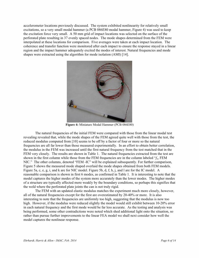
accelerometer locations previously discussed. The system exhibited nonlinearity for relatively small excitations, so a very small modal hammer (a PCB 086E80 modal hammer, Figure 4) was used to keep the excitation force very small. A 50 mm grid of impact locations was selected on the surface of the perforated plate resulting in 37 evenly spaced nodes. The mode shapes determined from the FEM were interpolated at these locations for comparison. Five averages were taken at each impact location. The coherence and transfer function were monitored after each impact to ensure the response stayed in a linear region and the impact hammer adequately excited the modes of interest. Natural frequencies and mode shapes were extracted using the algorithm for mode isolation (AMI) [14].

Figure 4: Miniature Modal Hammer (PCB 086E80)

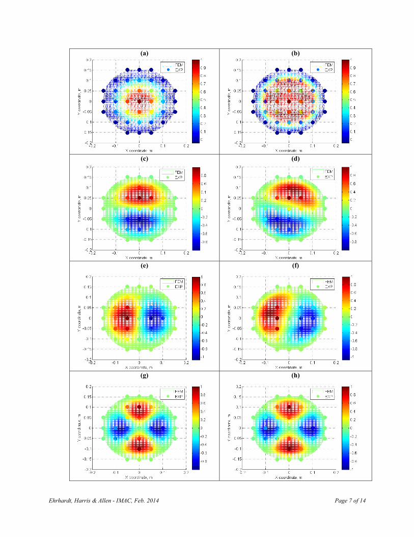
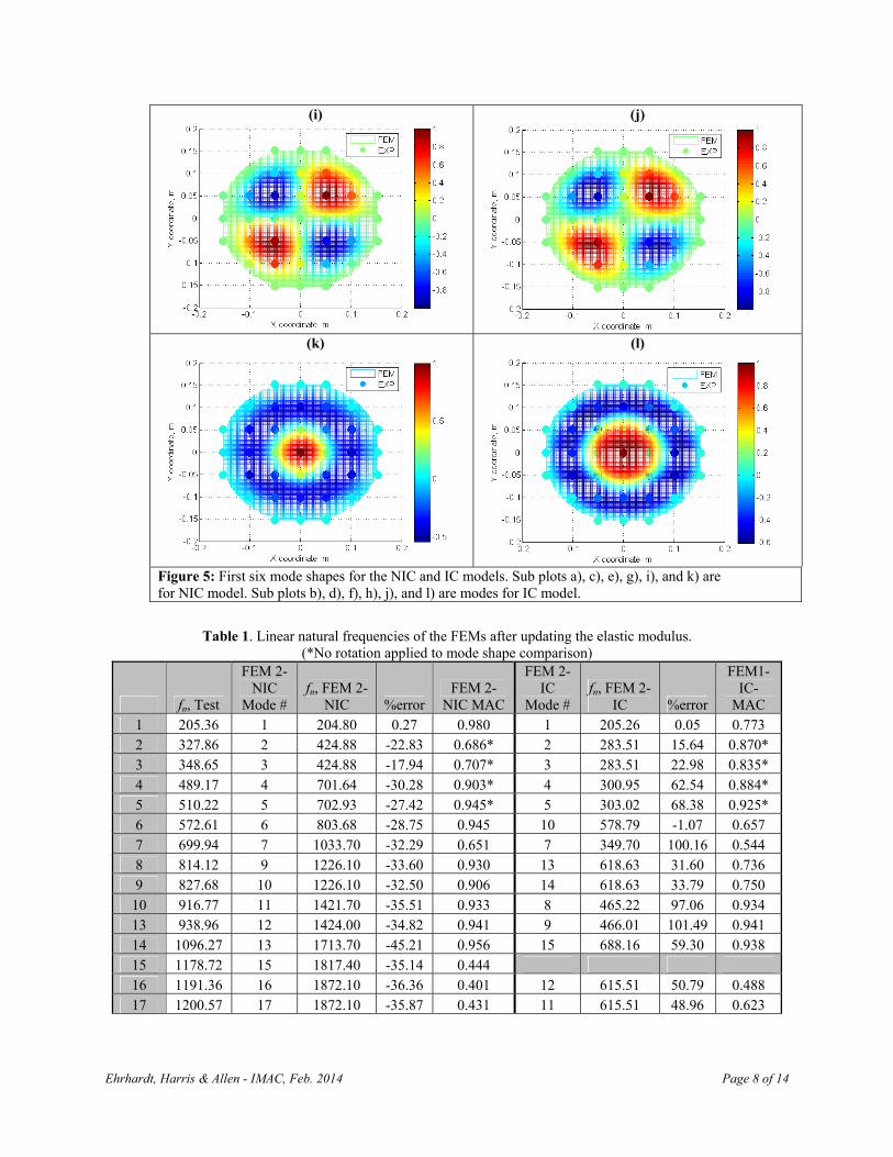
The natural frequencies of the initial FEM were compared with those from the linear modal test revealing revealed that, while the mode shapes of the FEM agreed quite well with those from the test, the reduced modulus computed from [10] seems to be off by a factor of four or more so the natural frequencies are all far lower than those measured experimentally. In an effort to obtain better correlation, the modulus in the FEM was increased until the first natural frequency from the test matched that in the FEM very closely. The results are shown in Table 1. The natural frequencies extracted from the test are shown in the first column while those from the FEM frequencies are in the column labeled “fn, FEM NIC.” The other columns, denoted “FEM -IC” will be explained subsequently. For further comparison, Figure 5 shows the measured mode shaped overlaid the mode shapes obtained from both FEM models. Figure 5a, c, e, g, i, and k are for NIC model. Figure 5b, d, f, h, j, and l are for the IC model. A reasonable comparison is shown in first 6 modes, as confirmed in Table 1. It is interesting to note that the model captures the higher modes of the system more accurately than the lower modes. The higher modes of a structure are typically affected more weakly by the boundary conditions, so perhaps this signifies that the weld where the perforated plate joints the can is not truly rigid. The FEM with an updated elastic modulus matches the experiment much more closely, however, all of the natural frequencies except for the first are overestimated by 20-40% or more. It is also interesting to note that the frequencies are uniformly too high, suggesting that the modulus is now too high. However, if the modulus were reduced slightly the model would still exhibit between 10-20% error in each natural frequency and the first mode would be far less accurate. As the testing and analysis was being performed, some other contradictions were noted which shed additional light onto the situation, so rather than pursue further improvements to the linear FEA model we shall next consider how well the model captures the nonlinear response.


(a) (b)

(c) (d)

(e) (f)

(g) (h)


(i) (j)

(k) (l)

Figure 5: First six mode shapes for the NIC and IC models. Sub plots a), c), e), g), i), and k) are for NIC model. Sub plots b), d), f), h), j), and l) are modes for IC model.

Table 1. Linear natural frequencies of the FEMs after updating the elastic modulus. (*No rotation applied to mode shape comparison)

fn, Test

FEM 2- NIC

Mode # fn, FEM 2-

NIC %error FEM 2-

NIC MAC

FEM 2- IC

Mode # fn, FEM 2-

IC %error

FEM1-IC-

MAC 1 205.36 1 204.80 0.27 0.980 1 205.26 0.05 0.773 2 327.86 2 424.88 -22.83 0.686* 2 283.51 15.64 0.870* 3 348.65 3 424.88 -17.94 0.707* 3 283.51 22.98 0.835* 4 489.17 4 701.64 -30.28 0.903* 4 300.95 62.54 0.884* 5 510.22 5 702.93 -27.42 0.945* 5 303.02 68.38 0.925* 6 572.61 6 803.68 -28.75 0.945 10 578.79 -1.07 0.657 7 699.94 7 1033.70 -32.29 0.651 7 349.70 100.16 0.544 8 814.12 9 1226.10 -33.60 0.930 13 618.63 31.60 0.736 9 827.68 10 1226.10 -32.50 0.906 14 618.63 33.79 0.750

10 916.77 11 1421.70 -35.51 0.933 8 465.22 97.06 0.934 13 938.96 12 1424.00 -34.82 0.941 9 466.01 101.49 0.941 14 1096.27 13 1713.70 -45.21 0.956 15 688.16 59.30 0.938 15 1178.72 15 1817.40 -35.14 0.444 16 1191.36 16 1872.10 -36.36 0.401 12 615.51 50.79 0.488 17 1200.57 17 1872.10 -35.87 0.431 11 615.51 48.96 0.623


3.2 Nonlinear Comparison

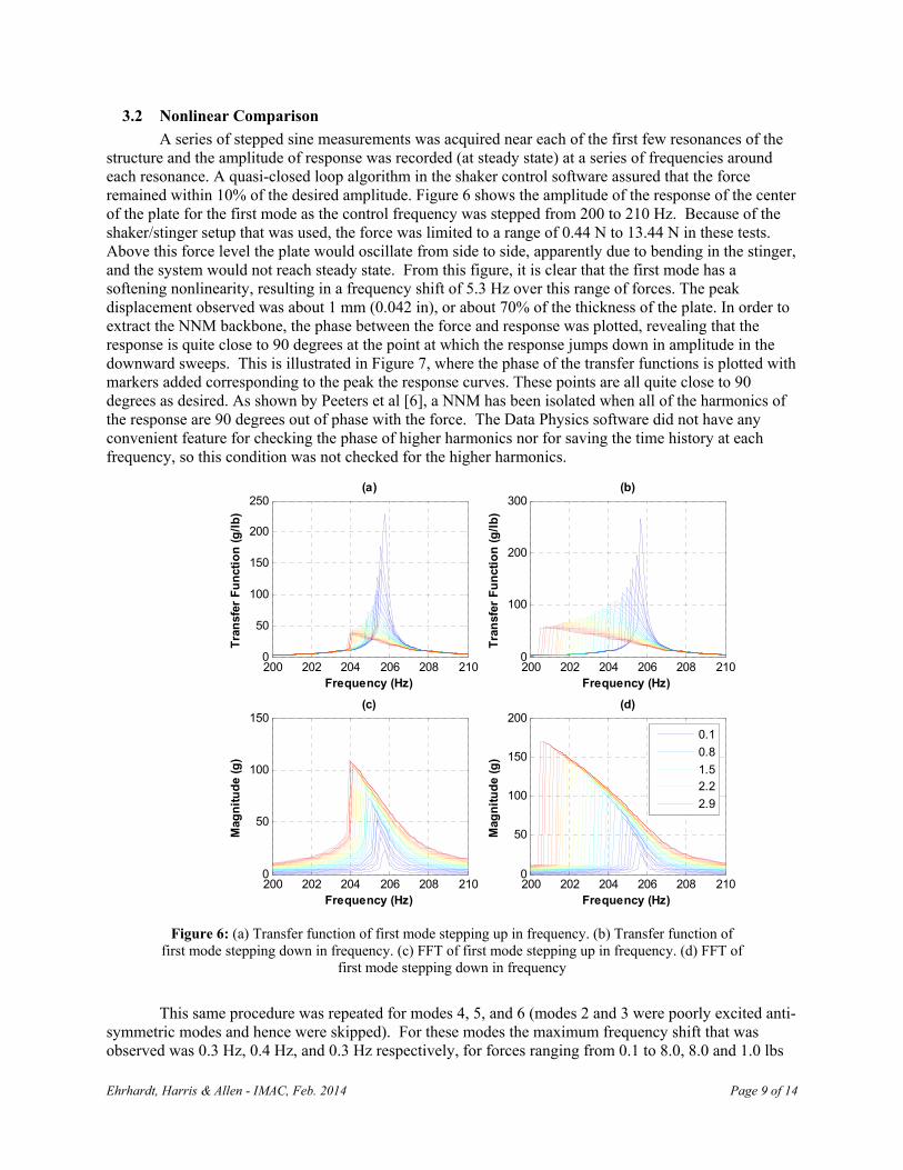
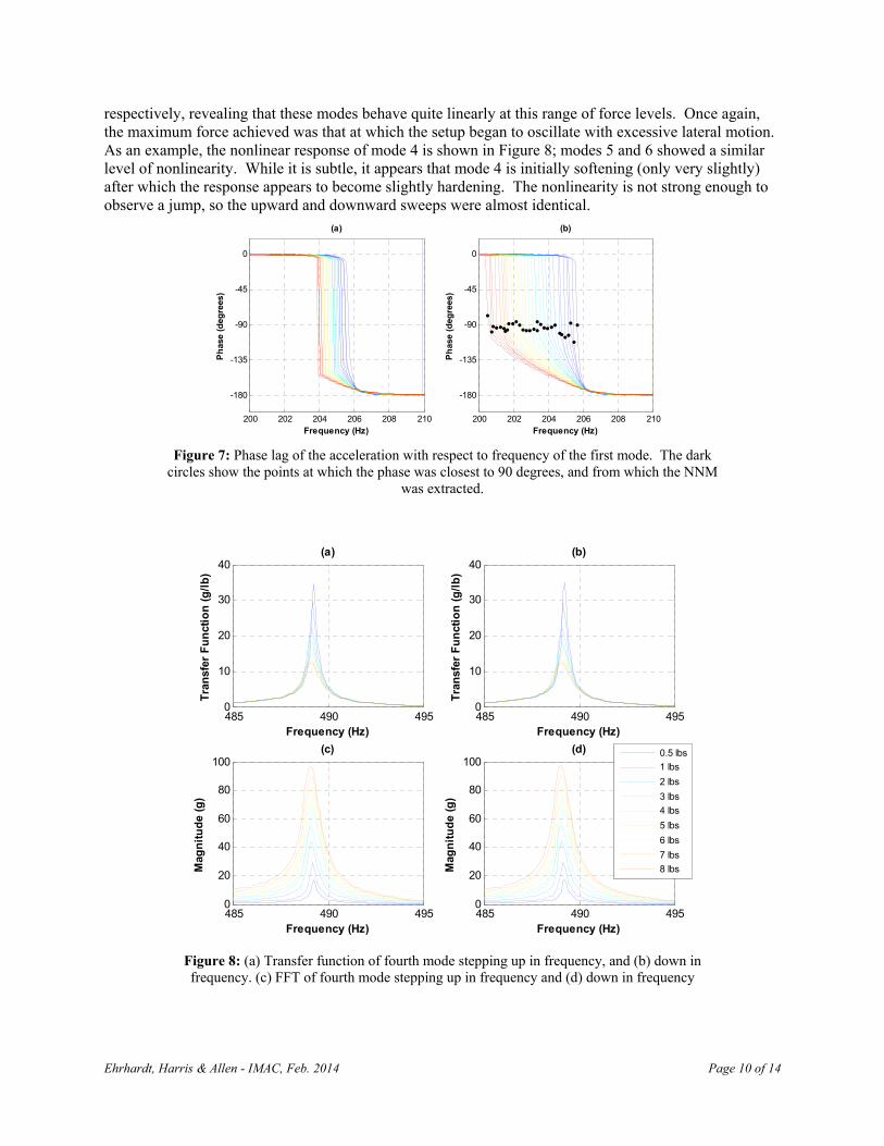
A series of stepped sine measurements was acquired near each of the first few resonances of the structure and the amplitude of response was recorded (at steady state) at a series of frequencies around each resonance. A quasi-closed loop algorithm in the shaker control software assured that the force remained within 10% of the desired amplitude. Figure 6 shows the amplitude of the response of the center of the plate for the first mode as the control frequency was stepped from 200 to 210 Hz. Because of the shaker/stinger setup that was used, the force was limited to a range of 0.44 N to 13.44 N in these tests. Above this force level the plate would oscillate from side to side, apparently due to bending in the stinger, and the system would not reach steady state. From this figure, it is clear that the first mode has a softening nonlinearity, resulting in a frequency shift of 5.3 Hz over this range of forces. The peak displacement observed was about 1 mm (0.042 in), or about 70% of the thickness of the plate. In order to extract the NNM backbone, the phase between the force and response was plotted, revealing that the response is quite close to 90 degrees at the point at which the response jumps down in amplitude in the downward sweeps. This is illustrated in Figure 7, where the phase of the transfer functions is plotted with markers added corresponding to the peak the response curves. These points are all quite close to 90 degrees as desired. As shown by Peeters et al [6], a NNM has been isolated when all of the harmonics of the response are 90 degrees out of phase with the force. The Data Physics software did not have any convenient feature for checking the phase of higher harmonics nor for saving the time history at each frequency, so this condition was not checked for the higher harmonics.

200 202 204 206 208 2100

50

100

150

200

250(a)

Frequency (Hz)

Tra

nsf

er F

un

ctio

n (

g/l

b)

200 202 204 206 208 2100

100

200

300(b)

Frequency (Hz)

Tra

nsf

er F

un

ctio

n (

g/l

b)

200 202 204 206 208 2100

50

100

150(c)

Frequency (Hz)

Mag

nit

ud

e (g

)

200 202 204 206 208 2100

50

100

150

200(d)

Frequency (Hz)

Mag

nit

ud

e (g

)

0.1

0.8

1.52.2

2.9

Figure 6: (a) Transfer function of first mode stepping up in frequency. (b) Transfer function of

first mode stepping down in frequency. (c) FFT of first mode stepping up in frequency. (d) FFT of first mode stepping down in frequency

This same procedure was repeated for modes 4, 5, and 6 (modes 2 and 3 were poorly excited anti-symmetric modes and hence were skipped). For these modes the maximum frequency shift that was observed was 0.3 Hz, 0.4 Hz, and 0.3 Hz respectively, for forces ranging from 0.1 to 8.0, 8.0 and 1.0 lbs


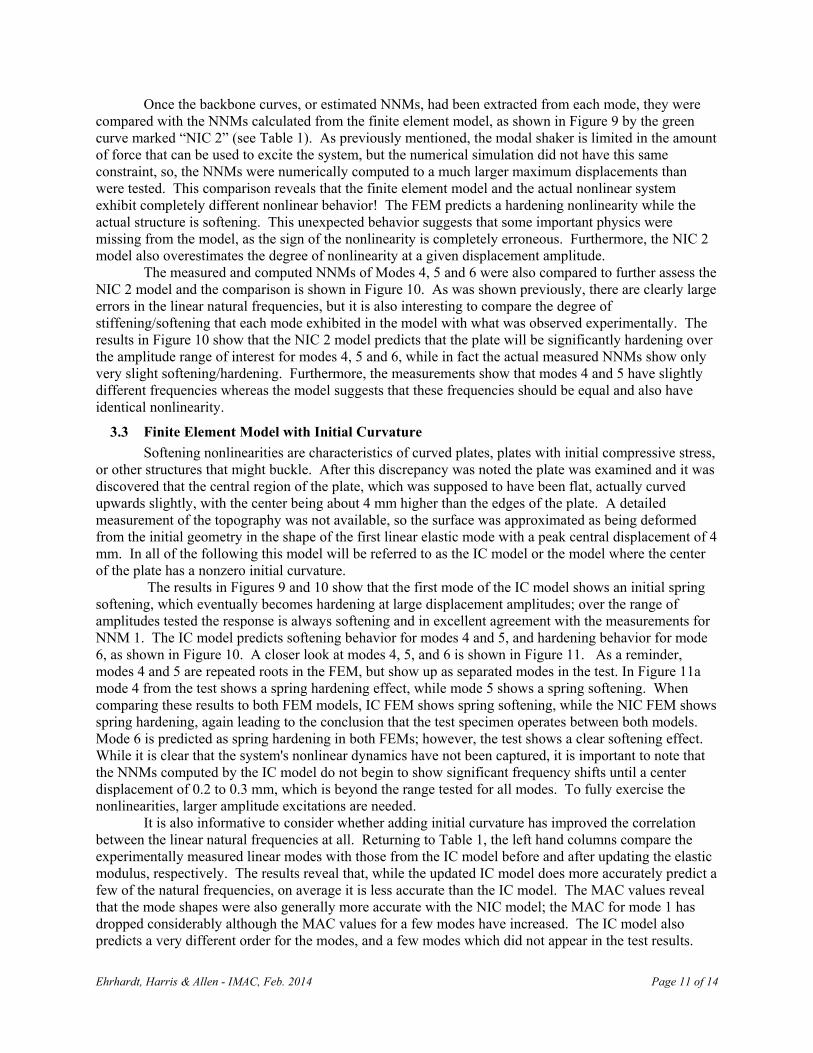
respectively, revealing that these modes behave quite linearly at this range of force levels. Once again, the maximum force achieved was that at which the setup began to oscillate with excessive lateral motion. As an example, the nonlinear response of mode 4 is shown in Figure 8; modes 5 and 6 showed a similar level of nonlinearity. While it is subtle, it appears that mode 4 is initially softening (only very slightly) after which the response appears to become slightly hardening. The nonlinearity is not strong enough to observe a jump, so the upward and downward sweeps were almost identical.

200 202 204 206 208 210

-180

-135

-90

-45

0

(a)

Frequency (Hz)

Ph

ase

(deg

rees

)

200 202 204 206 208 210

-180

-135

-90

-45

0

(b)

Frequency (Hz)

Ph

ase

(deg

rees

)

Figure 7: Phase lag of the acceleration with respect to frequency of the first mode. The dark

circles show the points at which the phase was closest to 90 degrees, and from which the NNM was extracted.

485 490 4950

10

20

30

40(a)

Frequency (Hz)

Tra

nsf

er F

un

ctio

n (

g/l

b)

485 490 4950

10

20

30

40(b)

Frequency (Hz)

Tra

nsf

er F

un

ctio

n (

g/l

b)

485 490 4950

20

40

60

80

100(c)

Frequency (Hz)

Mag

nit

ud

e (g

)

485 490 4950

20

40

60

80

100(d)

Frequency (Hz)

Mag

nit

ud

e (g

)

0.5 lbs

1 lbs

2 lbs

3 lbs

4 lbs

5 lbs

6 lbs

7 lbs

8 lbs

Figure 8: (a) Transfer function of fourth mode stepping up in frequency, and (b) down in frequency. (c) FFT of fourth mode stepping up in frequency and (d) down in frequency


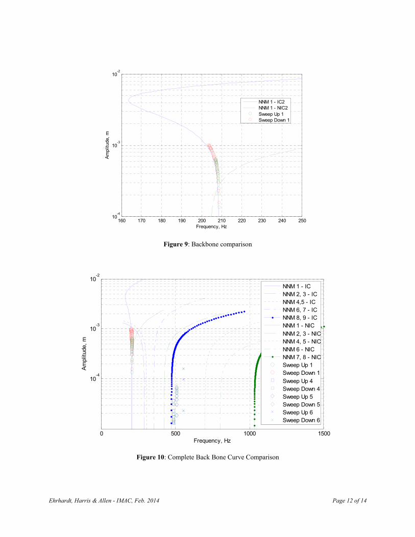
Once the backbone curves, or estimated NNMs, had been extracted from each mode, they were compared with the NNMs calculated from the finite element model, as shown in Figure 9 by the green curve marked “NIC 2” (see Table 1). As previously mentioned, the modal shaker is limited in the amount of force that can be used to excite the system, but the numerical simulation did not have this same constraint, so, the NNMs were numerically computed to a much larger maximum displacements than were tested. This comparison reveals that the finite element model and the actual nonlinear system exhibit completely different nonlinear behavior! The FEM predicts a hardening nonlinearity while the actual structure is softening. This unexpected behavior suggests that some important physics were missing from the model, as the sign of the nonlinearity is completely erroneous. Furthermore, the NIC 2 model also overestimates the degree of nonlinearity at a given displacement amplitude. The measured and computed NNMs of Modes 4, 5 and 6 were also compared to further assess the NIC 2 model and the comparison is shown in Figure 10. As was shown previously, there are clearly large errors in the linear natural frequencies, but it is also interesting to compare the degree of stiffening/softening that each mode exhibited in the model with what was observed experimentally. The results in Figure 10 show that the NIC 2 model predicts that the plate will be significantly hardening over the amplitude range of interest for modes 4, 5 and 6, while in fact the actual measured NNMs show only very slight softening/hardening. Furthermore, the measurements show that modes 4 and 5 have slightly different frequencies whereas the model suggests that these frequencies should be equal and also have identical nonlinearity.

3.3 Finite Element Model with Initial Curvature

Softening nonlinearities are characteristics of curved plates, plates with initial compressive stress, or other structures that might buckle. After this discrepancy was noted the plate was examined and it was discovered that the central region of the plate, which was supposed to have been flat, actually curved upwards slightly, with the center being about 4 mm higher than the edges of the plate. A detailed measurement of the topography was not available, so the surface was approximated as being deformed from the initial geometry in the shape of the first linear elastic mode with a peak central displacement of 4 mm. In all of the following this model will be referred to as the IC model or the model where the center of the plate has a nonzero initial curvature.

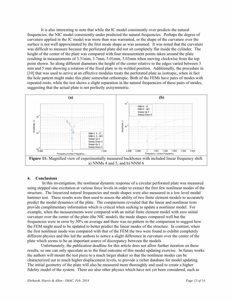
The results in Figures 9 and 10 show that the first mode of the IC model shows an initial spring softening, which eventually becomes hardening at large displacement amplitudes; over the range of amplitudes tested the response is always softening and in excellent agreement with the measurements for NNM 1. The IC model predicts softening behavior for modes 4 and 5, and hardening behavior for mode 6, as shown in Figure 10. A closer look at modes 4, 5, and 6 is shown in Figure 11. As a reminder, modes 4 and 5 are repeated roots in the FEM, but show up as separated modes in the test. In Figure 11a mode 4 from the test shows a spring hardening effect, while mode 5 shows a spring softening. When comparing these results to both FEM models, IC FEM shows spring softening, while the NIC FEM shows spring hardening, again leading to the conclusion that the test specimen operates between both models. Mode 6 is predicted as spring hardening in both FEMs; however, the test shows a clear softening effect. While it is clear that the system's nonlinear dynamics have not been captured, it is important to note that the NNMs computed by the IC model do not begin to show significant frequency shifts until a center displacement of 0.2 to 0.3 mm, which is beyond the range tested for all modes. To fully exercise the nonlinearities, larger amplitude excitations are needed.

It is also informative to consider whether adding initial curvature has improved the correlation between the linear natural frequencies at all. Returning to Table 1, the left hand columns compare the experimentally measured linear modes with those from the IC model before and after updating the elastic modulus, respectively. The results reveal that, while the updated IC model does more accurately predict a few of the natural frequencies, on average it is less accurate than the IC model. The MAC values reveal that the mode shapes were also generally more accurate with the NIC model; the MAC for mode 1 has dropped considerably although the MAC values for a few modes have increased. The IC model also predicts a very different order for the modes, and a few modes which did not appear in the test results.


160 170 180 190 200 210 220 230 240 25010

-4

10-3

10-2

Frequency, Hz

Am

plitu

de,

m

NNM 1 - IC2NNM 1 - NIC2Sweep Up 1Sweep Down 1

Figure 9: Backbone comparison

0 500 1000 1500

10-4

10-3

10-2

Frequency, Hz

Am

plitu

de,

m

NNM 1 - ICNNM 2, 3 - ICNNM 4,5 - ICNNM 6, 7 - ICNNM 8, 9 - IC NNM 1 - NIC

NNM 2, 3 - NICNNM 4, 5 - NICNNM 6 - NICNNM 7, 8 - NICSweep Up 1Sweep Down 1

Sweep Up 4Sweep Down 4Sweep Up 5Sweep Down 5Sweep Up 6Sweep Down 6

Figure 10: Complete Back Bone Curve Comparison


It is also interesting to note that while the IC model consistently over predicts the natural frequencies, the NIC model consistently under predicted the natural frequencies. Perhaps the degree of curvature applied in the IC model was more than was warranted, or the shape of the curvature over the surface is not well approximated by the first mode shape as was assumed. It was noted that the curvature was difficult to measure because the perforated plate did not sit completely flat inside the cylinder. The height of the center of the plate was compared with four measurement points taken around the plate resulting in measurements of 3.31mm, 3.7mm, 5.01mm, 5.03mm when moving clockwise from the top point shown. So along different diameters the height of the center relative to the edges varied between 3 mm and 5 mm showing a rotation of the fixed plate in its welded position. Additionally, the procedure in [10] that was used to arrive at an effective modulus treats the perforated plate as isotropic, when in fact the hole pattern might make this plate somewhat orthotropic. Both of the FEMs have pairs of modes with repeated roots, while the test shows a slight separation in the natural frequencies of these pairs of modes, suggesting that the actual plate is not perfectly axisymmetric.

(a)

0.995 1 1.00510

-6

10-5

10-4

Frequency/Linear Frequency, -

Am

plitu

de,

m

NNM 4, 5 - ICNNM 4, 5 - NICSweep Up 4Sweep Down 4Sweep Up 5Sweep Down 5

(b)

0.998 0.999 1 1.001 1.002 1.003 1.004 1.005

10-4

10-3

Frequency / Linear Frequency, -

Am

plitu

de,

x

NNM 6 - ICNNM 6 - NICSweep Up 6Sweep Down 6

Figure 11: Magnified view of experimentally measured backbones with included linear frequency shift.

a) NNMs 4 and 5, and b) NNM 6

4. Conclusions In this investigation, the nonlinear dynamic response of a circular perforated plate was measured using stepped sine excitation at various force levels in order to extract the first few nonlinear modes of the structure. The linearized natural frequencies and mode shapes were also measured in a low level modal hammer test. These results were then used to assess the ability of two finite element models to accurately predict the modal dynamics of the plate. The comparisons revealed that the linear and nonlinear tests provide complimentary information which is critical when seeking to update a nonlinear model. For example, when the measurements were compared with an initial finite element model with zero initial curvature over the center of the plate (the NIC model), the mode shapes compared well but the frequencies were in error by 30% on average and there was no pattern in the comparison to suggest how the FEM might need to be updated to better predict the linear modes of the structure. In contrast, when the first nonlinear mode was compared with that of the FEM the two were found to exhibit completely different physics and this led the authors to notice a slight difference in curvature over the center of the plate which seems to be an important source of discrepancy between the models. Unfortunately, the publication deadline for this article does not allow further iteration on these results, so one can only speculate as to the final outcome of this model updating exercise. In future works the authors will mount the test piece to a much larger shaker so that the nonlinear modes can be characterized out to much higher displacement levels, to provide a richer database for model updating. The initial geometry of the plate will also be measured more thoroughly and used to create a higher fidelity model of the system. There are also other physics which have not yet been considered, such as


the residual stresses caused by the formation of the plate and the added perforations and perhaps in the end these factors will need to be considered to fully characterize the nonlinear behavior of this system. The NNMs of the structure might also be quite sensitive to the ambient temperature, as that will change the distribution of initial stresses in the plate, so that should also be considered. Acknowledgements

The authors gratefully acknowledge the support of the Air Force Office of Scientific Research under grant number FA9550-11-1-0035, administered by the Dr. David Stargel of the Multi-Scale Structural Mechanics and Prognosis Program. They also wish to thank Peter Penegor and David Nickel for providing the perforated plate samples.

References [1] G. Kerschen, M. Peeters, J. C. Golinval, and A. F. Vakakis, "Nonlinear normal modes. Part I. A

useful framework for the structural dynamicist," Mechanical Systems and Signal Processing, vol. 23, pp. 170-94, 2009.

[2] R. J. Kuether, M. R. Brake, and M. S. Allen, "Evaluating Convergence of Reduced Order Models Using Nonlinear Normal Modes," presented at the 32nd International Modal Analysis Conference (IMAC XXXII), Orlando, Florida, 2014.

[3] M. Peeters, R. Viguie, G. Serandour, G. Kerschen, and J. C. Golinval, "Nonlinear normal modes, part II: toward a practical computation using numerical continuation techniques," Mechanical Systems and Signal Processing, vol. 23, pp. 195-216, 2009.

[4] M. S. Allen, R. J. Kuether, B. Deaner, and M. W. Sracic, "A Numerical Continuation Method to Compute Nonlinear Normal Modes Using Modal Reduction," presented at the 53rd AIAA Structures, Structural Dynamics, and Materials Conference, Honolulu, Hawaii, 2012.

[5] R. J. Kuether and M. S. Allen, "A Numerical Approach to Directly Compute Nonlinear Normal Modes of Geometrically Nonlinear Finite Element Models," Mechanical Systems and Signal Processing, vol. Submitted, 2013.

[6] M. Peeters, G. Kerschen, and J. C. Golinval, "Dynamic testing of nonlinear vibrating structures using nonlinear normal modes," Journal of Sound and Vibration, vol. 330, pp. 486-509, 2011.

[7] M. Peeters, G. Kerschen, and J. C. Golinval, "Modal testing of nonlinear vibrating structures based on nonlinear normal modes: Experimental demonstration," Mechanical Systems and Signal Processing, vol. 25, pp. 1227-1247, 2011.

[8] R. J. Kuether and M. S. Allen, "Computing Nonlinear Normal Modes Using Numerical Continuation and Force Appropriation," presented at the ASME 2012 International Design Engineering Technical Conferences IDETC/CIE 2012, Chicago, IL, 2012.

[9] A. W. Leissa, "Vibration of Plates," NASA, Ed., ed. Washington, D.C.: U.S. Government Printing Office, 1969.

[10] M. J. J. a. J. C. Jo, "Equivalent Material Properties of Perforated Plate with Triangular or Square Penetration Pattern for Dynamic Analysis," Nuclear Engineering and Technology, vol. 38, October 2006 2006.

[11] R. W. Gordon and J. J. Hollkamp, "Reduced-order Models for Acoustic Response Prediction," Air Force Research Laboratory, Dayton, OH2011.

[12] J. J. Hollkamp and R. W. Gordon, "Reduced-order models for nonlinear response prediction: Implicit condensation and expansion," Journal of Sound and Vibration, vol. 318, pp. 1139-1153, 2008.

[13] J. J. Hollkamp, R. W. Gordon, and S. M. Spottswood, "Nonlinear modal models for sonic fatigue response prediction: a comparison of methods," Journal of Sound and Vibration, vol. 284, pp. 1145-63, 2005.

[14] M. S. Allen, "Global and Multi-Input-Multi-Output (MIMO) Extensions of the Algorithm of Mode Isolation (AMI)," Ph.D. Ph.D., George W. Woodruff School of Mechanical Engineering, Georgia Institute of Technology, Atlanta, Georgia, 2005.

Documents

Numerical and Experimental Determination of Nonlinear ...sd.engr.wisc.edu/.../10/Ehrhardt-Harris-Allen-NLCumminsPlate-IMAC20… · Ehrhardt, Harris & Allen - IMAC, Feb. 2014 Page