NUMERICAL ASSESSMENT OF REINFORCED CONCRETE MEMBERS RETROFITTED WITH FIBER REINFORCED POLYMER FOR RESISTING BLAST

LOADING

By

GRAHAM LONG

A THESIS PRESENTED TO THE GRADUATE SCHOOL OF THE UNIVERSITY OF FLORIDA IN PARTIAL FULFILLMENT

OF THE REQUIREMENTS FOR THE DEGREE OF MASTER OF ENGINEERING

UNIVERSITY OF FLORIDA

2012

1

© 2012 Graham Long

2

To my family and friends

3

ACKNOWLEDGMENTS

I would like to express my sincere gratitude to Dr. Theodor Krauthammer for his

advice and direction facilitating the completion of this research. I would also like to

thank Dr. Serdar Astarlioglu for his support in the completion of this research. Finally, I

would like to thank the Canadian Armed Forces and 1 ESU (1st Engineer Support Unit)

for providing me with the opportunity to complete my graduate studies in structural

engineering.

4

TABLE OF CONTENTS page

ACKNOWLEDGMENTS .................................................................................................. 4 

LIST OF TABLES ............................................................................................................ 7 

LIST OF FIGURES .......................................................................................................... 8 

LIST OF ABBREVIATIONS ........................................................................................... 10 

ABSTRACT ................................................................................................................... 15 

CHAPTER

1 INTRODUCTION ................................................................................................ 16 

Problem Statement ............................................................................................. 16 Objective and Scope .......................................................................................... 17 Research Significance ........................................................................................ 18 

2 BACKGROUND LITERATURE REVIEW ........................................................... 19 

Dynamic Structural Analysis Suite (DSAS) ......................................................... 19 Blast Loading ...................................................................................................... 19 Materials ............................................................................................................. 21 

Concrete .................................................................................................. 21 Compressive stress-strain curve ................................................... 21 Tensile stress-strain curve ............................................................ 23 

Steel......................................................................................................... 24 Fiber Reinforced Polymers (FRP) ............................................................ 25 

Dynamic Analysis ............................................................................................... 27 Equivalent SDOF System ........................................................................ 28 

Equivalent mass ............................................................................ 28 Equivalent loading function ........................................................... 29 

Resistance Function ................................................................................ 30 Numerical Integration ............................................................................... 31 

Flexural Behavior ................................................................................................ 33 Diagonal Shear Behavior .................................................................................... 34 Rate Effects ........................................................................................................ 35 Fiber Reinforced Polymers ................................................................................. 37 

FRP Flexural Behavior ............................................................................. 37 FRP Shear Behavior ................................................................................ 38 FRP Rate Effects ..................................................................................... 38 FRP Size Effects ...................................................................................... 39 Debonding Behavior ................................................................................ 39 

Shear stress .................................................................................. 40 

5

Normal stress ................................................................................ 42 Mixed mode initiation .................................................................... 43 Effective bond length ..................................................................... 45 Ultimate bond strength .................................................................. 46 

Load-Impulse (P-I) Diagrams.............................................................................. 47 

3 METHODOLOGY ............................................................................................... 58 

Structural Overview ............................................................................................ 58 Debonding Behavior ........................................................................................... 59 DSAS Overall Algorithm ..................................................................................... 61 

4 ANALYSIS .......................................................................................................... 65 

Material Model Validation ................................................................................... 65 Debonding Validation ......................................................................................... 66 Dynamic loading ................................................................................................. 67 Parametric Study ................................................................................................ 68 

FRP Ultimate Strength ............................................................................. 69 FRP Elastic Modulus................................................................................ 69 FRP Thickness ........................................................................................ 69 FRP Width ............................................................................................... 70 

5 SUMMARY AND CONCLUSIONS ..................................................................... 80 

Limitations .......................................................................................................... 80 Future Development /Recommendations ........................................................... 81 General Conclusions .......................................................................................... 83 

REFERENCE LIST........................................................................................................ 85 

BIOGRAPHICAL SKETCH ............................................................................................ 89 

6

LIST OF TABLES

Table page 4-1 Beam material properties for experimental test case .......................................... 78 

4-2 DSAS inputs for material model verification ....................................................... 78 

4-3 Peak results of unstrengthen static loading case. ............................................... 78 

4-4 Peak results of FRP strengthened static loading case ....................................... 79 

4-5 Material data for parametric case studies ........................................................... 79 

7

LIST OF FIGURES

Figure page 2-1 Free field pressure time variation ....................................................................... 48 

2-2 Modified Hognestad stress-strain curve for concrete in compression. ................ 48 

2-3 Confined concrete stress strain curve ................................................................ 49 

2-4 Tensile stress strain curve for reinforced concrete ............................................. 49 

2-5 Steel Stress-strain curve model. ......................................................................... 50 

2-6 Deformation profile for a beam ........................................................................... 50 

2-7 SDOF inelastic resistance model ........................................................................ 51 

2-8 Stress strain diagram for reinforced concrete beam ........................................... 52 

2-9 Shear reduction model ....................................................................................... 53 

2-11 Section forces for FRP reinforced concrete beam .............................................. 55 

2-14 Typical response functions ................................................................................. 57 

3-1 Test beam from study. ........................................................................................ 62 

3-2 Comparison of debonding process. .................................................................... 62 

3-3 DSAS debonding algorithm ................................................................................ 63 

3-4 Overall DSAS algorithm ...................................................................................... 64 

4-1 Validation of the material model of DSAS. .......................................................... 71 

4-2 Load-displacement curve for validation of the debonding model in DSAS. ........ 72 

4-3 Moment-curvature model for validation of the debonding model in DSAS. ......... 73 

4-4 Time-displacement response to blast loading case. ........................................... 73 

4-5 Pressure-impulse curve under uniform blast loading. ......................................... 74 

4-6 Effect of FRP Yield Strength. .............................................................................. 75 

4-7 Effect of FRP Modulus of Elasticity. .................................................................... 76 

4-8 Effect of FRP thickness. ..................................................................................... 77 

8

4-9 Effect of FRP width. ............................................................................................ 78 

9

LIST OF ABBREVIATIONS

Aci Area of concrete at each layer

Asi Area of steel at each layer

bc Concrete width

bf FRP width

c Neutral axis depth

C Damping coefficient

dsi Depth of steel layer

D” Nominal diameter of hoops

D’ Nominal diameter of longitudinal compression reinforcement

Ead Adhesive modulus of elasticity

Ec Elastic modulus of concrete

Enhc Concrete enhancement factor in compression

Enhct Concrete enhancement factor in tension

Enhs Steel enhancement factor

Ef FRP modulus of elasticity

Es Steel modulus of elasticity

F Force

f’c Compressive strength of concrete

fci Stress of concrete layer

Fci Concrete layer forces

Fe Equivalent Force

ft Tensile strength

fs Steel stress

10

fsi Stress of steel layer

Fsi Steel layer forces

fu Ultimate steel stress

fy Steel yield stress

f”y Yield stress of the hoops/stirrups

Gf FRP interfacial fracture energy

Gn Normal interfacial fracture energy

Gs Shear interfacial fracture energy

GT Total interfacial fracture energy

h Concrete section depth

H” Average core dimension of the confined concrete compression area

is Impulse

K Stiffness

Ke Resistance factor

KL Load factor

Km Mass factor

l Length

Le Effective bond length

Lb Bond length

M Mass

mci Concrete layer moment

Me Equivalent mass

Mfl Ultimate moment capacity due only to flexure

11

Mn Moment at mid-span

msi Steel layer moment

Mt Total mass

Mu Ultimate moment capacity due only to shear

Pso Incident pressure

Pu Bond strength

tad Thickness of adhesive layer

tf Thickness of FRP

to Time of positive Phase

R Resistance function

Rm Maximum resistance

Re Equivalent resistance function

s Hoop spacing

sn Normal stress slip

snf Slip at maximum normal stress

ss Shear stress slip

ssf Slip at final debonding

sso Slip at maximum shear stress

SRF Shear reduction factor

u1 Axial displacement of member

u2 Axial displacement of debonded section

u Displacement

u& Velocity

12

u&& Acceleration

w Uniformly distributed load

w1 Vertical displacement of member

w2 Vertical displacement of debonded section

Y1 Distance from debonded interface to member neutral axis

Y2 Distance from debonded interface to debonded section neutral axis

x Position

zi Depth of concrete layer

β Newmark-Beta constant

βl Effective bond length factor

βw Bond width ratio factor

Δ Increment space

δ Deflection

ε Total Strain

εc Concrete Strain

εs Steel strain

εsh Strain hardening in steel

εf Final strain in steel

ε& Strain rate

sε& Quasi-static strain rate

ρ” Web reinforcement ratio

ϕ Shape function

blα Blast loading decay coefficient

13

nσ Normal shear stress

τ Interfacial shear stress

maxτ Max interfacial shear stress

14

15

Abstract of Thesis Presented to the Graduate School of the University of Florida in Partial Fulfillment of the

Requirements for the Degree of Master of Engineering

NUMERICAL ASSESSMENT OF REINFORCED CONCRETE MEMBERS RETROFITTED WITH FRP FOR RESISTING BLAST LOADING

By

Graham Long

May 2012

Chair: Theodore Krauthammer Major: Civil Engineering

The use of fiber reinforced polymers for the retrofit of existing structures is a

common practice in blast protection. The tools used to assess the behavior of structures

have become more refined allowing for precise modeling of reinforced members

retrofitted with fiber reinforced polymers (FRP). However, many of these tools require

extensive computational power that is often time consuming. This study aims to adapt

an existing expedient dynamic analysis assessment tool in order to account for the

behavior of reinforced concrete members retrofitted with FRP for flexural enhancement.

FRP retrofits have been shown to increase the capacity of the members under severe

loading conditions. However, the strength associated with the FRP layer is not always

able to fully develop due to the debonding behavior between the two surfaces. The

model will seek to capture this behavior by employing fracture mechanics along the

bonded interface. The results of the modeling tool will be validated by comparing them

to those of finite element analysis programs as well as available experimental test data.

An additional parametric study will be conducted to evaluate the models ability to

capture the bond behavior when adjusting the properties associated with the FRP.

CHAPTER 1 INTRODUCTION

Problem Statement

The vulnerability of many existing structures has been demonstrated by the

various incidents over the last half century. Many of these structures were not designed

to withstand severe loading due to an explosive loading incidents. As a result, there

has been a requirement to increase the blast resistance for other critical infrastructure

systems in order to preserve life and operations. While extensive studies were

conducted on the various means for retrofitting existing structures under normal service

and seismically-induced loading, it is only within the last two decades that the research

has expanded to include severe short duration loading cases. The choice on which

method to use often depends on a variety of factors. While different facilities will have

different governing factors, the factor that continually is expressed is the cost to

effectiveness ratio. For this reason, the use of externally bonded fiber reinforced

polymer (FRP) strips or mats have been identified as a suitable option due to its high

strength to weight ratio. In addition, the ease of application allows for the retrofit to be

completed in a timely manner.

The employment of FRP along the tension face allows for an initial increase in

beam flexural strength while reducing the deflection. However, the effectiveness of the

FRP retrofit is limited by the bond strength. In most cases, the FRP will debond from

the beam before the it reaches its ultimate strength. It is therefore important to model

the bond and the debonding behavior in order to accurately determine the effectiveness

of a retrofit.

16

Extensive design calculations are often required for determining the full effect of

these severe load cases on structural members and the means to counteract the effect.

The use of an advanced finite element method is computationally expensive and may

not be suitable in time sensitive situations. Conversely, the use of design guidelines

provides methods that do not require extensive analysis to design against specific

threats but may not apply to all cases. In addition, these guidelines are often

conservative and may produce results that may not be cost efficient due to conservative

limits. Therefore, an approach that combines a high level of accuracy as well as utilizes

a simplified analysis method to minimize computational time is required to produce

accurate results when time is limited. Dynamic Structural Analysis Suite (DSAS) is a

computer program that has been under development for many years and has had

extensive research completed on reinforced concrete structural members. However,

retrofitting these structures with new composite materials has not been incorporated into

that research and further work needs to be done to develop an expedient algorithm to

account for these new methods.

Objective and Scope

The objective of this research project is to develop an algorithm that is both

computationally expedient and sufficiently accurate for the purpose of analyzing

reinforced concrete beams retrofitted with externally bonded fiber reinforced polymer

(FRP) strips subjected to severe short dynamic loading. The research project will be

completed in the following steps:

• Develop an algorithm to evaluate the flexural and deformation responses of reinforced concrete members retrofitted with externally bonded fiber reinforced polymer strips on the tension face of the member and implement this algorithm as a new module in DSAS.

17

• Validate the algorithm model in and the results obtained in DSAS to available experimental data.

• Complete a parametric study using DSAS to fully understand the effect of FRP layer on reinforced concrete members subjected to severe short duration load cases, by comparing their behavior with and without the retrofit. Various thicknesses and strengths of the FRP layer will also be examined to determine the effect on debonding and flexural enhancement.

Research Significance

The algorithm to be developed in this study will be incorporated into the computer

code, DSAS, in order further develop the resistance function of the components. DSAS

will then have the capability to assess the response of reinforced concrete retrofitted

with externally bonded fiber reinforced polymer strips.

18

CHAPTER 2 BACKGROUND LITERATURE REVIEW

This chapter will provide a review of the concepts and studies associated with the

behavior of reinforced concrete members retrofitted with FRP. The topics will include a

look at the structural analysis process employed by the Dynamic Structural Analysis

Suite as well as the characteristics and behaviors associated with externally bonded

FRP materials. The material is based on a review of recent studies and publications in

the field of protective structures and fiber reinforced polymer.

Dynamic Structural Analysis Suite (DSAS)

DSAS is a multifunctional program that is capable of modeling the response of a

wide range of structural components under both static and dynamic loads (Chee et al.

2008; Tran et al. 2009; Morency et al. 2010). It has the capability to perform time-

history and load-impulse (P-I) analyses by employing accurate resistance functions that

can be derived for the various structural elements in its library. This program utilizes a

combination of advanced fully-nonlinear and Physics-based structural behavioral

models for expedient structural behavior computations.

Blast Loading

Blast loading is a shockwave caused by a sudden release of energy from an

explosive device. In the case of an air blast at ground level, the shockwave is

simultaneously reflected off the ground and the wave expands out in a hemispherical

configuration. The loading produced from this shockwave can be assumed to be

uniformly distributed over the entire structural member, except when the point of

initiation is extremely close to the structure. In which case, advanced computational

fluid dynamic (CFD) simulations are required to determine the complicated interaction

19

between the blast wave and a structure. The loading time history can be illustrated

using the free field pressure-time variation obtained from TM 5-855-1 (1986) by means

of Krauthammer (2008) and is illustrated in Figure 2-1. Loading due blast is

characterized by an initial peak overpressure that decays over time based on a decay

coefficient. The loading will consist of two phases, positive and negative.

Loading due to a blast and impact is characterized by the peak overpressure, the

duration, and the impulse. In order to determine the pressure on the structure as a

function of time, the modified Friedlander equation will be used in order to minimize the

computational demand instead of other more precise equations.

( )blt

oso e

ttPtP α/1)( −⋅

⎥⎥⎦

⎤

⎢⎢⎣

⎡⎟⎟⎠

⎞⎜⎜⎝

⎛−⋅= (2-1)

The impulse can be obtained by the area enclosed by the load-time curve.

∫=ot

s dttPi0

)( (2-2)

Where is the incident over pressure. soP

ot is the positive phase duration.

blα is the decay coefficient.

si is the positive impulse.

The negative phase loading is much smaller than the positive phase loading and is

often omitted in dynamic analysis. In addition, the positive phase is often idealized as a

triangular load for simplified calculations.

20

Materials

Concrete

Concrete is a non-homogenous material composed of cement and aggregates

mixed with water. The combined effects of incorporating the materials results in a non-

linear material behavior as the concrete develops cracks. Concrete is much stronger in

compression than in tension.

Compressive stress-strain curve

Concrete compressive strength is typically evaluated using uniaxial compression

tests on plain concrete cylinders. The modified Hognestad stress-strain curve, as

shown in Figure 2-2, is commonly used to represent unconfined concrete in

compression. It consists of a second degree parabola for the ascending branch

followed by a linear descending branch.

The ascending branch, for 0εε ≤c

⎥⎥⎦

⎤

⎢⎢⎣

⎡⎟⎟⎠

⎞⎜⎜⎝

⎛−=

2

00

" 2εε

εε cc

cc ff

(2-3)

The descending branch, for

0038.00 thanlessandc εε >

( )0" εε −−= ccdcc Eff (2-4)

where is the concrete compressive stress. cf

cc ff '" 9.0= is the maximum concrete compressive stress. (2-5)

cf ' is the uniaxial concrete compressive strength under standard test cylinder.

cε is the concrete strain.

c

c

Ef "

08.1

=ε is the concrete strain at maximum compressive stress. (2-6)

21

Elastic modulus is given in ACI Committee 318 (2008) by Equation 2-7 and 2-8. cE

ccc fwE '335.1= for (2-7) 33 /160/90 ftlbwftlb c ≤≤

cc fE '57000= for normal weighted concrete with in psi. (2-8) cf '

Descending elastic modulus, is given by Equation 2-7. cdE

ksiorf

E ccd 500

0038.0"15.0

0ε−= (2-9)

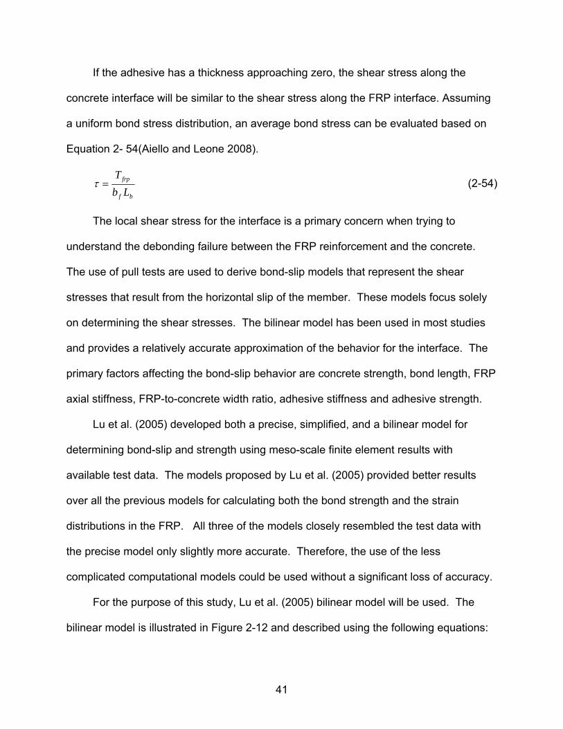
For confined concrete, Krauthammer et al. (1988) outlines a material model that

incorporates the effects due to the expanding concrete being restrained by lateral

reinforcement. Figure 2-3 illustrates the material model. Due to the dependence on the

core dimensions, the values calculated will be readjusted as the neutral axis changes

during analysis.

The ascending branch, for 0εε ≤c

⎟⎟⎠

⎞⎜⎜⎝

⎛⋅⎟⎟⎠

⎞⎜⎜⎝

⎛−

′⋅⋅

+

⎟⎟⎠

⎞⎜⎜⎝

⎛⋅−⎟⎟

⎠

⎞⎜⎜⎝

⎛⋅⎟⎟⎠

⎞⎜⎜⎝

⎛ ⋅

=

0

0

00

0

21εεε

εε

εεε

c

c

c

ccc

c

fKE

KE

f

(2-10)

The descending branch, for Kc 3.00 εεε ≤≤

⎥⎥⎦

⎤

⎢⎢⎣

⎡⎟⎟⎠

⎞⎜⎜⎝

⎛−⋅⋅−⋅′⋅= 18.01

00 εε

ε ccc ZfKf (2-11)

The steady state, for cK εε ≤3.0

cc fKf ′⋅⋅= 3.0 (2-12)

⎟⎟

⎠

⎞

⎜⎜

⎝

⎛

′

′′⋅⋅⎟⎟⎠

⎞⎜⎜⎝

⎛⋅⎟⎠⎞

⎜⎝⎛

′′−⋅+=

c

yr

f

fs

hρ

ε 734.01005.00024.00 (2-13)

22

c

yr

f

fDD

hsK

′

′′⋅⎟⎠⎞

⎜⎝⎛ ′⋅

′′′

+⋅⎟⎠⎞

⎜⎝⎛

′′⋅−⋅+= ρρ245.010091.01 (2-14)

002.01000

002.0343

5.0

−⎟⎟⎠

⎞⎜⎜⎝

⎛−′

′⋅++

′′⋅⋅

=

c

cr f

fsh

Zρ

(2-15)

H ′′ is the average core dimension of the confined concrete compression zone, measured to the outside of the stirrups.

rρ is the confining steel volume to the confined concrete core volume per unit

length of the element in compression zone. ρ ′ is the longitudinal compression reinforcement ratio.

yf ′′ is the yield stress of the hoops.

is the spacing of the hoops. s

D ′′ is the nominal diameter of the hoops.

D′ is the nominal diameter of the longitudinal compression reinforcement.

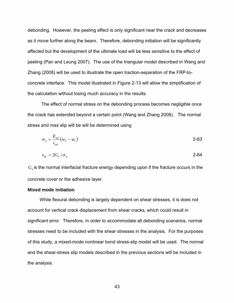
Tensile stress-strain curve

Concrete has a low tensile strength compared to its compressive strength and its

strength is based on either the splitting tensile strength or the modulus of rupture. The

behavior of concrete in tension is a two phase model. Initially, the model is linear up to

the failure point at which point cracking occurs. At this point, there is a significant drop

in strength but the concrete retains some residual strength and the concrete model

follows a curved softening path. Hsu (1993) described the tensile stress- strain curve of

concrete as follows and is illustrated in Figure 2-4:

Ascending branch, for crc εε ≤

ccc Ef ε= (2-16)

23

cc fE '47000= (2-17)

Descending branch, for crc εε ≥

4.0

⎟⎟⎠

⎞⎜⎜⎝

⎛=

c

crcrc ff

εε

(2-18)

ccr ff '75.3= (2-19)

crf is the concrete cracking stress of plain concrete in pounds per square inch.

crε is the cracking strain.

Steel

The steel reinforcement is strong in tension and is used to add ductility to the

concrete member. There are different steel stress-strain models available that can

encompass elastic and perfectly plastic behavior, as well as strain hardening. The

model outline in Park and Pauley (1975) outlines all three of these behavior

characteristics and is illustrated in Figure 2-5 follows the three stages according to the

following procedure.

for ys εε ≤

yss Ef ε⋅= (2-20)

for shys εεε ≤≤

ys ff = (2-21)

for shs εε ≥

( )( )

( ) ( )( ) ⎥

⎦

⎤⎢⎣

⎡

−+⋅

−⋅−+

+−⋅+−⋅

⋅= 2130260

2602

rmm

ff shs

shs

shsys

εεεεεε (2-22)

24

( )2

2

15

160130

r

rrff

m y

u

⋅

−⋅−+⋅⋅⎟⎟⎠

⎞⎜⎜⎝

⎛

= (2-23)

sE is the steel modulus of elasticity.

sε is the steel strain.

shε is the strain at the commencement of steel hardening.

suε is the ultimate steel strain.

fε is the final steel strain.

sf is the steel stress.

uf is the ultimate steel stress.

yf is the steel yielding stress.

Fiber Reinforced Polymers (FRP)

FRP strengthened members has exhibited significantly higher load-carrying

capacity and stiffness. Depending on the system type, thickness, fiber angle orientation

and geometry, load capacity increases can range between 1.5 to 5 times that of an

unstrengthen member (Kachlakev et al. 2000). The most common FRP utilizes

unidirectional fibers oriented along the longitudinal length. Multi-direction weaved mats

can also be used to provide strength in two directions. Moreover, the use of

unidirectional plies can also be layered in order to achieve two-directional strength.

FRP material is strong in tension, but is weak in compression. The compression

strength is based on the epoxy. While not as strong as steel, it can improve the

member’s strength without substantial structural weight increases. Most studies have

assumed FRP to be linearly elastic up to failure. This assumption will also be

25

incorporated into this study. However, individual product information would be needed

to predict behavior of a reinforced structure due to the various different manufacturing

techniques and processes.

Environmental conditions and long-term loading can significantly weaken the

material properties. The materials are subjected to creep and fatigue when

experiencing long loading periods reducing the effectiveness of the bond behavior

between the fibers and the epoxy matrix. Furthermore, moisture content, UV radiation

temperature effects, and chemical reactions can further degrade the strength of the

member.

Fibers are the load carrying components of the composite materials and occupy a

large volume of the overall laminate. Fibers are available in various materials such as

glass, carbon, aramid and boron. Glass fibers tend to be more ductile than Carbon

fibers but will have a lower ultimate tensile strength. Because these products are

proprietary materials, they tend to have specific characteristics that can alter the

predicted behavior. Therefore, it is important to obtain all the material data sheets for

the purpose obtaining the best results.

Epoxy and resin materials can serve multiple purposes when applied to FRP. A

primer is used to prepare any surface before attaching the FRP material. This allows

for better adhesion and reduces the risk of poor bonds. Adhesives attach to

components together and are used when attaching FRP strips. Saturants impregnate

the fiber matrix and are used when performing a wet-layup reinforcing of fibers.

Epoxies have low tensile strength when compared to fibers but have good ductility.

26

Thick epoxy layers will be subject to excessive deformation when loaded reducing the

ability of the fiber to transmit its tensile strength to the member.

Dynamic Analysis

The dynamic analysis of either a multi-degree of freedom system or a single

degree of freedom system can be represented by the same equation of motion:

)()( tFuRuCuM =++ &&& (2-24)

M is the mass acting on inertia of the system.

C is the damping coefficient.

)(uR is the stiffness function. is the forcing function. )(tF

u is the displacement.

u& is the velocity.

u&& is the acceleration.

The resistance function R(u) will often be replaced by Ku for the purposes of

dynamic analysis when the system being evaluated is linearly elastic. The resistance

function will be discussed further in a later section.

Rigorous analysis is often computationally expensive and is only truly feasible

when the resistance and load functions are represented by convenient mathematical

functions. As such, an approximate method is often used for analysis of the structure

when only a localized evaluation of deflection is required. This requires the idealization

of the structure and the loading. Equivalent values for the mass (Me), the resistance

function (Re(u)), and the forcing function (Fe(t)) are developed using shape functions as

described in Biggs (1964) and Krauthammer et al. (1988).

27

Equivalent SDOF System

SDOF analyses are often used due to their computational efficiency. However,

many of the structural members that need to be analyzed are continuous such as

beams and slabs. In order to analyze them as a single degree of freedom system, the

member will need to be transformed into an equivalent system. The process outlined in

Biggs (1964) allows for the determination of the transverse displacement of the member

at various points along the member by use of a shape function φ(x) derived by the

application of static loads. This assumes that the calculated equivalent SDOF

displaced shape is equal to that of the real structure at the same time. However, the

stresses and forces are not directly equivalent to those of the real structure. Since this

method accounts for only the elastic and plastic domains with ideal boundary

conditions, alternate means are required to obtain a more accurate representation of an

equivalent system. Krauthammer et al. (1988) modifies this model by taking into

account the transition phases between the two domains and is valid for all boundary

conditions. Figure 2-6 illustrates the deformation profile that can be represented by the

shape function.

Equivalent mass

The equivalent mass of the structure is derived by balancing the kinetic energy of

the moving parts of the beam for both the real and the equivalent system. Equating the

two systems will provide the following equivalent mass relationship.

∫=L

e dxxxmM0

2 )()( ϕ (2-25)

From which, the equivalent mass factor can be derived from a ratio of the

equivalent mass to the total mass.

28

tem MMK /= (2-26)

Both of these will be affected at each time step in dynamic analysis due to the

change in the shape profile of the member. Krauthammer et al. (1988) uses the

following linear interpolation procedure to calculate the equivalent mass factor at each

time step. However, the equivalent mass will remain constant during hinge formation,

since there is only a minor effect on the inelastic deformed shape function.

)()1(

)1(i

ii

miimmim uu

uuKK

KK −⋅−

−+=

+

+ (2-27)

The use of the DSAS program eliminates the need for the equivalent mass factor

by calculating an equivalent mass function for each step based on displacements.

Using finite elements, an equivalent mass is generated with the following relationship:

∑ ⎟⎟⎠

⎞⎜⎜⎝

⎛=

Nnodes

j imid

iji

jie d

dMM

2

(2-28)

Where i is the load increment and j is the node location along the beam.

Equivalent loading function

The equivalent forcing function is derived in a similar way as the equivalent mass.

It is derive by balancing the external work for both the real and equivalent systems.

Equating the two systems will provide the following equivalent loading relationship.

(2-29) [∫ ∑ ⋅+=L

i iie xtxFdxtxtxpF0

)(),(),(),( ϕϕ ]

From which, the equivalent loading factor can be derived from a ratio of the

equivalent load to the total load.

teL FFK /= (2-30)

29

The same approach was used for computing the equivalent load factor at each

time step as was used for the equivalent mass factor.

)()1(

)1(i

ii

LiiLLiL uu

uuKK

KK −⋅−

−+=

+

+ (2-31)

The use of the DSAS program eliminates the need for the equivalent loading factor

by calculating an equivalent loading function for each step based on displacements.

Applying the same approach as the equivalent mass, an equivalent resistance function

is generated using the following function:

ie

Nnodes

j imid

iji

ji

e Rdd

fF ==∑ (2-32)

From which an equivalent loading function can be developed.

)()()(

),( twuwuF

tuF ee = (2-33)

Where w is the static load that would result in the control displacement.

Resistance Function

The resistance function represents the restoring force a member exhibits to return

to its initial condition when subjected to an external load. Biggs (1964) suggests that,

for most structures, a simplification can be made using a bilinear function to compute

the resistance factor using the maximum plastic-limit load as the maximum resistance

Rm for the function. In addition, the resistance factor KR must always equal the load

factor KL. However, a majority of the cases that will be discussed require further

development of the resistance function since the members being evaluated have

nonlinear characteristics.

30

For dynamic analysis cases, the effect of load reversal needs to be considered in

the resistance function model. The Krauthammer et al. (1988) model expands on the

Sozen (1974) model by including all material and support nonlinearities in a piecewise,

multilinear curve. Figure 2-7 illustrates the modified resistance-displacement model

compared to the bilinear model. If the maximum dynamic displacement does not

exceed the yield point at A or A’, the behavior will remain elastic and will oscillate about

zero displacement. However, if the maximum dynamic displacement exceeds the yield

point, plastic deformation will occur and the member will have a residual displacement

once it comes to rest. If point C is exceeded, the member will have failed in flexure.

Otherwise, the member will unload according to the path outlined in the model.

While the resistance of beams and one-way slabs can be analyzed using the

method previously describe, two way slabs need to be analyzed by calculating the

resistance in both directions and super positioning the resistance functions to obtain the

total system resistance model. In addition, if the section is not symmetrical, a different

resistance model will be required for load reversal.

Numerical Integration

Due to the nonlinear characteristics of the members that will be evaluated, a

closed form solution may not be possible. As such, a numerical solution that is valid for

a wide range of cases is required. The approach used to numerically integrate the

equation of motion is chosen in order to minimize computational demands while still

providing accuracy. Either an implicit or explicit time step can be used to evaluate the

system. The implicit method evaluates the equation of motion at the next time step

while an explicit method evaluates it at the current time step. While an implicit method

is computationally expensive for a MDOF system, it is feasible for a SDOF system. As

31

such, a modified Newmark-Beta method will be used for the purpose of this research.

The Equations 2-34 and 2-35 are used to compute the velocities and displacements for

this method.

( )tttttt uutuu Δ+Δ+ +⋅Δ

+= &&&&&&2

(2-34)

22

21 tututuuu ttttttt Δ⋅⋅+Δ⋅⋅⎟

⎠⎞

⎜⎝⎛ −+Δ⋅+= Δ+Δ+ &&&&& ββ (2-35)

The β is taken as 1/6 corresponding to the linear acceleration method as proposed

in Tedesco (1999) instead of 1/4 corresponding to the constant average acceleration

method originally proposed by Newmark (1962). The following steps are used in order

to solve for the equation of motion for the system.

• Use the known velocity and displacement at time t to calculate the acceleration at time t.

• Estimate the acceleration at the next time step.

• Compute both the velocity and the displacement at the next time step using the estimated acceleration value.

• Compute the acceleration at the next time step using the equation of motion and the computed velocity and displacement.

• Compare the computed acceleration to the estimated acceleration. If the convergence tolerance is achieved, continue on to the next time step. Otherwise, repeat the process using the calculated acceleration as the new estimate in step 2 of the process.

The level of accuracy and stability of the final result must be considered when

selecting a value of time step. Using a time step that is less than a tenth of the natural

period of the system will usual allow for a fast convergence. However, the time step

must also be small enough in order to account for the loading of the member. In order

to further improve the efficiency of the of the evaluation, a smaller time step can be

32

used during the loading phase of the system and a larger time step can be used during

the free vibration phase.

Flexural Behavior

Flexural behavior of reinforced concrete has been studied extensively since most

structural design is based on flexural failure (MacGregor 2009; Park and Gamble 2000).

The use of a Moment Curvature relationship is the primary method for representing

flexural behavior and its function is generated using strain compatibility and equilibrium.

Flexural Behavior in reinforced concrete is based on three assumptions.

• Sections perpendicular to the axis of bending that are plane before bending will remain plane after bending.

• The strain in reinforcement is equal to the strain in the concrete at the same level.

• The stresses in the concrete and reinforcement can be computed from the strains by using stress-strain curves for concrete and steel.

• For most cases, tension in concrete is ignored. However, in blast loading cases, the tension is included since the strain rate may have a significant effect on the tension strength of the concrete. The strain rate effects will be further discussed in a later section.

Figure 2-8 shows a stress strain diagram of a reinforced concrete beam cross

section under flexural loading. By dividing the section into layers, a more accurate

representation of the behavior can be achieved instead of using the Whitney stress

block which is the primary design method under normal loading conditions. The

moment-curvature diagram can be obtained by incrementing the curvature from zero to

failure and calculating the strain and stresses in each layer. An iterative process would

be used to ensure that equilibrium and compatibility are satisfied for each layer. The

stress-strain values for each material will be defined by individual predefined material

models. Both confined concrete and unconfined concrete will need to be considered.

33

Diagonal Shear Behavior

When a member fails in flexure, it is a combination of both the flexural behavior

and the diagonal shear behavior. It occurs when flexural stress and shear stress act

together such that there is a large enough stress to create cracks perpendicular to the

principle tensile stress along the member to prevent brittle failure. As such, the use of

web reinforcement is required. Due to the diagonal shear influence on the deflection of

beams, the use of a shear reduction factor is required in the analysis of the member.

Krauthammer et al. (1988) modified a shear reduction factor originally proposed by

Krauthammer et al. (1979) to account for deep and slender beams.

)( flu MMSRF = (2-36)

Krauthammer et al. (1979) used the relationships in Equations 2-37, 2-38, and 2-

39 to describe the minimum SRF ratio as a function of the tensile longitudinal

reinforcement ratio, ρ .

0.1:%65.00 =⎟⎟⎠

⎞⎜⎜⎝

⎛<<

mfl

u

MM

ρ (2-37)

)0065.0(6.360.1:%88.1%65.0 −−=⎟⎟⎠

⎞⎜⎜⎝

⎛≤< ρρ

mfl

u

MM (2-38)

6.0:%88.2%88.1 =⎟⎟⎠

⎞⎜⎜⎝

⎛≤<

mfl

u

MM

ρ (2-39)

The modified minimum moment capacity ratio with web reinforcement as proposed

by Krauthammer et al. (1988) identified by point 2P′ in Figure 2-9 is given Equation 2-40.

( )αtan0.1 ⋅⎥⎥⎦

⎤

⎢⎢⎣

⎡⎟⎟⎠

⎞⎜⎜⎝

⎛−+⎟

⎟⎠

⎞⎜⎜⎝

⎛=′⎟

⎟⎠

⎞⎜⎜⎝

⎛

mfl

u

mfl

u

mfl

u

MM

MM

MM (2-40)

34

Where the angle of compressive strut at ultimate is calculated for a deep

rectangular beam by )5.2/1( ≤≤ da

08.4)/(72.2 * +⋅⋅= daρα (2-41)

and a slender rectangular beam )7/5.2( ≤≤ da by

22.7)/(06.3 * +⋅⋅= daρα (2-42)

cy ff ′′′⋅′′= /* ρρ (2-43)

Where ρ ′′ is the web reinforcement ratio.

The computed moments are then multiplied by the SRF and the curvature is

divided by the SRF (Krauthammer 1988). This model is included in the DSAS program.

Rate Effects

Various studies have found that the strength and modulus of elasticity of concrete

and steel increase significantly when subjected to high loading rates such as impact and

blast Shanna (1991). Of the two techniques used in analysis, one is a dynamic

enhancement factor based on straining rate to increase the material properties used in

the derivation of moment-curvature, diagonal shear and direct shear relationships. The

other applies the enhancement factor directly to the resistance function by multiplying

the shear and flexure capacity of the section by the enhancement factor.

The use of either the strain rate, stress rate, or the loading rate can be used to

develop the enhancement factor. However, since the strain rate is the controlling

parameter for the development of the moment-curvature relationship, it will be used as

the independent parameter. Based on the DSAS program the following models are

used for the material enhancement factors. The use of Soroushian and Obaseki (1986)

35

model has been recommended by both Shanna (1991) and by Krauthammer et al.

(2002).

The enhancement factor for steel material is provided by Equation 2-45.

)()(

)()(

staticfdynamicf

staticfdynamicf

Enhu

u

y

ys == (2-44)

( )[ ]y

yys f

ffEnh

)log(05.065.02.11.3 ε&⋅⋅++⋅+= (2-45)

However, the Soroushian and Obaseki (1989) model underestimates the dynamic

increase factor for concrete in compression under high strain rates. Therefore, the

CEB-FIP (1990) model is used. The enhancement factor for concrete material is

provided by Equation 2-46 and 2-47.

)()(

staticfdynamicf

Enhc

cc ′

′= (2-46)

For 1sec30 −≤ε&

( ) αεε 026.1/ scEnh &&= (2-47)

For 1sec30 −>ε&

( ) 3/1/ scEnh εεγ &&= (2-48)

Where (quasi-static strain rate) 16 sec1030 −−= xsε&

)2156.6(10 −= αγ (2-49)

)1450/95/(1 cf ′+=α (2-50)

For concrete in tension, the model proposed by Ross et al. (1989) was used and is

given by Equation 2-51.

086.210 ))log7(0164.0( ε&+= eEnhct (2-51)

36

Fiber Reinforced Polymers

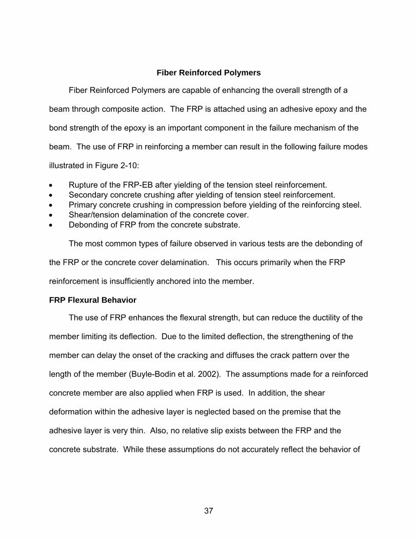
Fiber Reinforced Polymers are capable of enhancing the overall strength of a

beam through composite action. The FRP is attached using an adhesive epoxy and the

bond strength of the epoxy is an important component in the failure mechanism of the

beam. The use of FRP in reinforcing a member can result in the following failure modes

illustrated in Figure 2-10:

• Rupture of the FRP-EB after yielding of the tension steel reinforcement. • Secondary concrete crushing after yielding of tension steel reinforcement. • Primary concrete crushing in compression before yielding of the reinforcing steel. • Shear/tension delamination of the concrete cover. • Debonding of FRP from the concrete substrate.

The most common types of failure observed in various tests are the debonding of

the FRP or the concrete cover delamination. This occurs primarily when the FRP

reinforcement is insufficiently anchored into the member.

FRP Flexural Behavior

The use of FRP enhances the flexural strength, but can reduce the ductility of the

member limiting its deflection. Due to the limited deflection, the strengthening of the

member can delay the onset of the cracking and diffuses the crack pattern over the

length of the member (Buyle-Bodin et al. 2002). The assumptions made for a reinforced

concrete member are also applied when FRP is used. In addition, the shear

deformation within the adhesive layer is neglected based on the premise that the

adhesive layer is very thin. Also, no relative slip exists between the FRP and the

concrete substrate. While these assumptions do not accurately reflect the behavior of

37

FRP, they are necessary for computational efficiency. In addition, the degree of

inaccuracy does not have a significant effect on the flexural strength of the member.

The process for determining the moment-curvature of the reinforced member is

similar to that of a normal reinforced concrete member. However, the total strains in the

member are adjusted to account for the strain of the FRP on the bottom layer. Due to

the very small thickness of the FRP layer, it will be assumed to act in the same location

of the bottom layer of the concrete. As such, the strain of the FRP will be the same as

the strain acting on the bottom layer of concrete. Until debonding occurs, the FRP layer

will be considered another layer of tensile reinforcement.

FRP Shear Behavior

The use of FRP applied to the bottom layer of the concrete does not typically add

to the shear strength of the member (Kachlakev et al. 2000). Diagonal cracks still

develop at similar loading levels. However, the FRP allows the ability to maintain the

integrity of the member in the presence of a shear crack. Shear failure will then be

accompanied by the transverse rupture of the FRP composite. If there is a vertical

displacement, the peeling of the FRP membrane will need to be considered and will be

discussed in more detail in the debonding section of this review.

FRP Rate Effects

The strain-rate effect for a FRP plate when compared to those of concrete and

steel was found to be negligible according to Johnson et al. (2005). Therefore, it will not

be considered in the analysis of this study. However, rate effects will have an effect on

the bond strength of the FRP-to-concrete interface. This is attributed to the

dependence of bond strength on the concrete shear strength. Therefore, the rate

38

enhancement factor previously discussed will need to be applied to the concrete model

for tension.

FRP Size Effects

The amount of FRP applied to base of the member will need to be considered

when calculating the capacity. Higher FRP reinforcement ratios have lower deflection

capacities and higher stiffness. However, increasing the thickness of the FRP by using

multiple plys does not always lead to a higher member capacity. The studies performed

by Pham et al. (2004) and Maalaj et al. (2005) show that the effectiveness of the FRP is

reduced as the relative stiffness of FRP to steel increases. Maalaj et al. (2005) further

illustrates that the peak interfacial shear stresses seems to increase with increasing

FRP reinforcement. As a result, debonding will occur earlier in the loading process.

Debonding Behavior

Debonding will occur well below the rupture strain of the FRP, leading to an

underutilization of the strength of the reinforcement (Smith et al. 2010; Rougier et al.

2006). Debonding of the FRP from the concrete often occurs when the surface has not

properly been prepared. If the FRP is properly applied, various tests have shown that

the failure will not be at the concrete adhesive interface, but within the concrete cover

just above the adhesive layer. This is due to the shear strength of the adhesive layer

being higher than that of the concrete cover. The amount of the concrete cover that

delaminates will be dependent on the material properties within the concrete.

Debonding occurs at locations of high stress concentrations such as formed

cracks or at the ends of the FRP plate and is directly related to the shear stress

experience in the interfacial layer. Depending upon the location of failure, a specific set

of criteria will need to be satisfied. The common types of debonding failure include

39

plate-end debonding, mid-span debonding, and shear-span debonding. Plate-end

debonding depends largely on the interfacial shear and the normal stress concentration

at the cut-off points of the FRP plate. Once debonding occurs, the crack will propagate

towards the center of the member. The Mid-span debonding starts at regions of max

moment and usually propagates towards the nearest plate end. The higher interface

stresses are developed by the opening of a major crack and rely primarily on shear

stress concentrations. Shear span and intermediate shear crack debonding are

affected by crack widening as well as relative vertical displacement. The vertical

displacement causes a peeling effect on the FRP and influences the initiation of the

bond failure. Therefore, both normal and shear stresses influence the debonding

process. Once debonding has occurred, the behavior of the member will revert back to

that of the unstrengthened member (Pham 2004).

Shear stress

Shear Stress develops between the layers of a beam when subjected to a

difference in axial loading. In the case of a beam under flexural loading, the axial

loading in each section of the beam is based on the different strain values derived from

the curvature of the beam. Figure 2-11 shows the development of the shear stress

between the layers. Given an adhesive layer thickness, Equations 2-52 and 2-53

defines the shear stress within the adhesive layer assuming the strain varies linearly

across its depth (Li et al. 2009).

)(112 uu

taa −=γ (2-52)

aaa Gγτ = (2-53)

40

If the adhesive has a thickness approaching zero, the shear stress along the

concrete interface will be similar to the shear stress along the FRP interface. Assuming

a uniform bond stress distribution, an average bond stress can be evaluated based on

Equation 2- 54(Aiello and Leone 2008).

bf

frp

LbT

=τ (2-54)

The local shear stress for the interface is a primary concern when trying to

understand the debonding failure between the FRP reinforcement and the concrete.

The use of pull tests are used to derive bond-slip models that represent the shear

stresses that result from the horizontal slip of the member. These models focus solely

on determining the shear stresses. The bilinear model has been used in most studies

and provides a relatively accurate approximation of the behavior for the interface. The

primary factors affecting the bond-slip behavior are concrete strength, bond length, FRP

axial stiffness, FRP-to-concrete width ratio, adhesive stiffness and adhesive strength.

Lu et al. (2005) developed both a precise, simplified, and a bilinear model for

determining bond-slip and strength using meso-scale finite element results with

available test data. The models proposed by Lu et al. (2005) provided better results

over all the previous models for calculating both the bond strength and the strain

distributions in the FRP. All three of the models closely resembled the test data with

the precise model only slightly more accurate. Therefore, the use of the less

complicated computational models could be used without a significant loss of accuracy.

For the purpose of this study, Lu et al. (2005) bilinear model will be used. The

bilinear model is illustrated in Figure 2-12 and described using the following equations:

41

so

s

ss

maxττ = if (2-55) sos ss ≤

sosf

ssf

ssss

−

−= maxττ if (2-56) sfsso sss ≤<

0=τ if (2-57) sfs ss >

The final slip is calculated using Equation 2-58

max/2 τfsf Gs = (2-58)

The max shear stress and corresponding slip are given by Equations 2-59 and 2-60.

tw fβτ 50.1max = (2-59)

twso fs β0195.0= (2-60)

The interfacial fracture energy can be expressed as Equation 2-61.

twf fG 2308.0 β= (2-61)

The FRP-to-concrete width ratio factor can be derived by the following formula

proposed by Lu et al. (2005)

cf

cfw bb

bb/25.1/25.2

+

−=β (2-62)

fb is the width of FRP plate.

cb is width of concrete member.

tf is the tensile strength.

Normal stress

Cracks that experience both vertical and horizontal displacements will be

subjected to both peeling and pulling forces. The peeling force will generate normal

stresses acting perpendicular to the interface of the member increasing the ease of

42

debonding. However, the peeling effect is only significant near the crack and decreases

as it move further along the beam. Therefore, debonding initiation will be significantly

affected but the development of the ultimate load will be less sensitive to the effect of

peeling (Pan and Leung 2007). The use of the triangular model described in Wang and

Zhang (2008) will be used to illustrate the open traction-separation of the FRP-to-

concrete interface. This model illustrated in Figure 2-13 will allow the simplification of

the calculation without losing much accuracy in the results.

The effect of normal stress on the debonding process becomes negligible once

the crack has extended beyond a certain point (Wang and Zhang 2008). The normal

stress and max slip will be will be determined using

( 12 wwtE

ad

adn −=σ ) 2-63

nnnf Gs σ/2= 2-64

nG is the normal interfacial fracture energy depending upon if the fracture occurs in the

concrete cover or the adhesive layer.

Mixed mode initiation

While flexural debonding is largely dependent on shear stresses, it is does not

account for vertical crack displacement from shear cracks, which could result in

significant error. Therefore, in order to accommodate all debonding scenarios, normal

stresses need to be included with the shear stresses in the analysis. For the purposes

of this study, a mixed-mode nonlinear bond stress-slip model will be used. The normal

and the shear-stress slip models described in the previous sections will be included in

the analysis.

43

The slip for the of the normal and shear stresses can be derived using a

coordinate system and are represented by (Wang and Zhang, 2008):

12 wwsn −= (2-65)

222111 wYuwYuss ′−−′−= (2-66)

ns is the normal stress slip.

ss is the shear stress slip.

21 ,uu are the axial displacements of the member and the debonded section

21 , ww are the vertical displacements of the member and the debonded section

are the distances from debonding interface to neutral axis of each member 21 ,YY

For the purposes of this study, the normal and shear stresses will be treated as

independent since there is little experimental data outlining their interaction. This

assumption will allow for the simplification of the analysis and the level of error should

be minimal. Debonding will occur when the total fracture energy of the system is

reached. By combining the fracture energies of both the normal and shear stress slip

models, the total fracture energy developed at each stage of the evaluation can be

determined.

snT GGG += (2-67)

n

s

nnn dssGn

∫=0

σ (2-68)

s

s

ss dssGs

∫=0

τ (2-69)

Since the failure will likely occur in the concrete cover, the fractural energy will be

based on the concrete material properties. Using a simple linear debonding criteria

44

developed by Hutchinson and Suo (1991), full debonding will occur when the following

equation is satisfied.

1=+sc

s

nc

n

GG

GG (2-70)

As previously discussed, the effect on debonding due to normal stresses will

become insignificant after the crack propagates past a certain point. At that point,

debonding will be determined solely by shear stresses.

Effective bond length

Despite the FRP being applied to the entire member, only a small section closest

to the loading is used to determine the debonding process. Any bond length that

extends beyond the effective bond length does not add a significant value to the

strength of anchorage. As the crack propagates further away from the original loading,

the resistance in the FRP at a point further away becomes active against bond-slip.

Yuan et al. (2004) developed an effective length model for a bilinear bond-slip model

that will be used in this study.

( )( )a

aaLe221

221

1 tantanln

21

λλλλλλ

λ −+

+= (2-71)

ff tEs0

max1

τλ = (2-72)

fff tEss )( 0

max2 −=

τλ (2-73)

⎥⎥⎦

⎤

⎢⎢⎣

⎡ −=

f

f

sss

a 0

2

99.0arcsin1λ

(2-74)

45

The factor of 0.99 was used instead of the original value of 0.97 proposed by Yuan

et al. (2004) in order to achieve a closer agreement to model proposed by Chen and

Teng (2001). This percentage indicates the level of bond strength that is achieved in an

infinitely long bonded joint with the higher percentage providing the more stringent

definition.

The effective bond length defined by Yuan et al. (2004) can be applied to plate

end debonding. However, during beam flexure, intermediate crack induced debonding

can occur and would require a different anchorage length. Teng et al. (2003) identifies

the intermediate crack induced effective length in Equation 2-75. They further explain

that the anchorage bond length should be twice the size of the effective bond length.

c

ffe f

tEL

′= (2-75)

Ultimate bond strength

The ultimate bond strength is the maximum strength that can be sustained by the

shear interface up to a maximum limit when the bond length is equal to the effective

bond length. If the load is greater than the ultimate bond strength, the crack will

continue to propagate until such time that the load can be sustained by the remaining

bonded zone. Equation 2-76 obtained from Lu et al. (2005) predicts the ultimate bond

strength.

fffflu GtEbP 2β= (2-76)

where

⎟⎟⎠

⎞⎜⎜⎝

⎛=

e

bl L

L2

sinπ

β (2-77)

46

If the bond length is greater than the effective length, the bond length factor, lβ

,will be equal to one as no further bond strength is gained from additional anchorage.

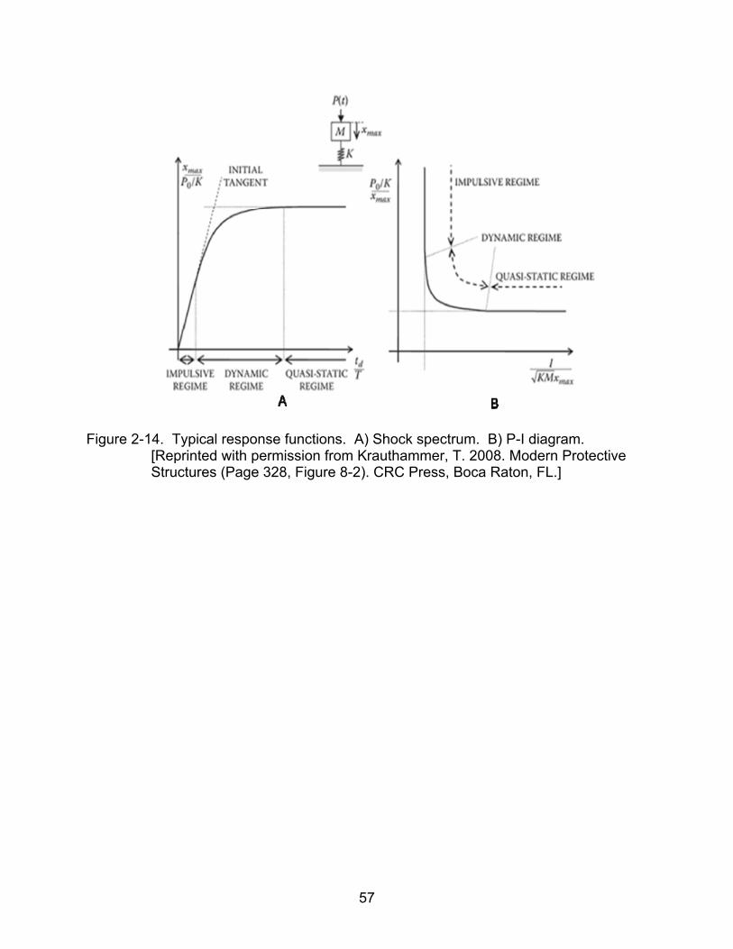
Load-Impulse (P-I) Diagrams

P-I Diagrams provide the means of determining the level of damage on a structure

or member. The points of the curve represent a pre-defined threshold response criteria

based on the equivalent peak load and impulse required to achieve the specific

behavior. Any combination of pressure and impulse that is below the curve is safe.

The curve is broken down into three separate regimes as illustrated in Figure 2-14.

The impulsive regime is characterized by loads of short duration where the maximum

response is not reached until the load duration is complete. The dynamic regime is

representative of the maximum response being reached close to the end of the loading

of the member. Finally, the quasi-static regime indicates when a member has reached

the maximum response before the loading has been removed. Krauthammer (2008)

outlines various methods for developing the curve. Simple problems allow for the use of

closed form solutions, while other cases make use of the energy balance method.

However, for complex problems such as those to be discussed during this research, a

numerical solution must be employed. Blasko et al. (2007) outlines the method that has

been employed in the DSAS program and which will be applied to this study.

47

Figure 2-1. Free field pressure time variation. [Reprinted with permission from Krauthammer, T. 2008. Modern Protective Structures (Page 68, Figure 3-1). CRC Press, Boca Raton, FL.]

Figure 2-2. Modified Hognestad stress-strain curve for concrete in compression.

48

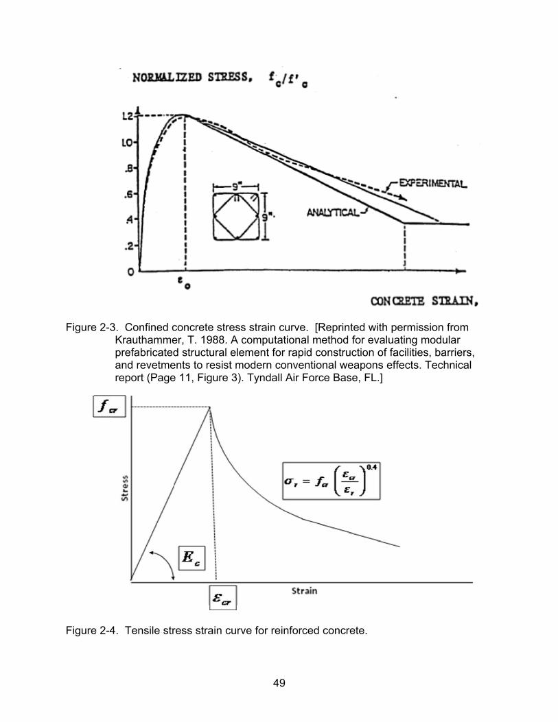
Figure 2-3. Confined concrete stress strain curve. [Reprinted with permission from Krauthammer, T. 1988. A computational method for evaluating modular prefabricated structural element for rapid construction of facilities, barriers, and revetments to resist modern conventional weapons effects. Technical report (Page 11, Figure 3). Tyndall Air Force Base, FL.]

Figure 2-4. Tensile stress strain curve for reinforced concrete.

49

Figure 2-5. Steel Stress-strain curve model.

Figure 2-6. Deformation profile for a beam.

50

Figure 2-7. SDOF inelastic resistance model. [Reprinted with permission from Krauthammer, T. 1988. A computational method for evaluating modular prefabricated structural element for rapid construction of facilities, barriers, and revetments to resist modern conventional weapons effects. Technical report (Page 103, Figure 38). Tyndall Air Force Base, FL.]

51

Figure 2-8. Stress strain diagram for reinforced concrete beam.

52

Figure 2-9. Shear reduction model. [Reprinted with permission from Krauthammer, T. 1988. A computational method for evaluating modular prefabricated structural element for rapid construction of facilities, barriers, and revetments to resist modern conventional weapons effects. Technical report (Page 37, Figure 12). Tyndall Air Force Base, FL.]

53

Figure 2-10. Failure modes of FRP reinforced concrete members. [Reprinted with permission from Teng, J.G. 2003. Intermediate crack-induced debonding in RC beams and slabs.(Page 448, Figure 1) Construction and Building Materials.]

54

Figure 2-11. Section forces for FRP reinforced concrete beam.

55

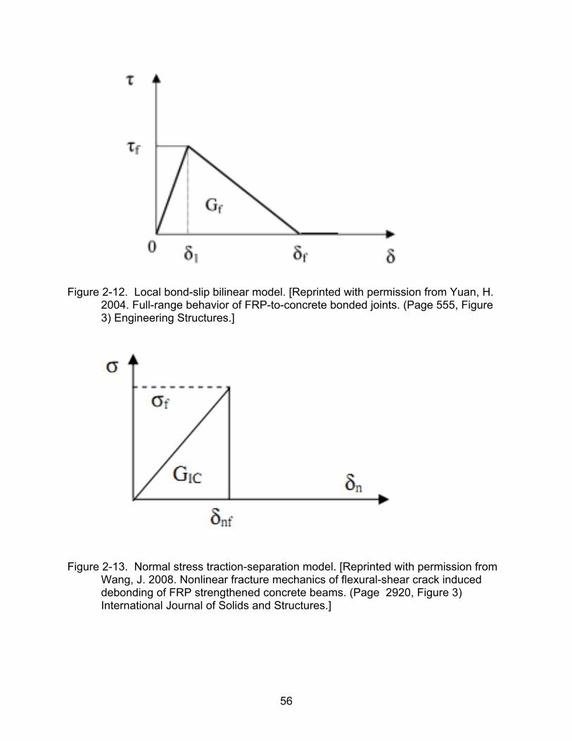
Figure 2-12. Local bond-slip bilinear model. [Reprinted with permission from Yuan, H. 2004. Full-range behavior of FRP-to-concrete bonded joints. (Page 555, Figure 3) Engineering Structures.]

Figure 2-13. Normal stress traction-separation model. [Reprinted with permission from Wang, J. 2008. Nonlinear fracture mechanics of flexural-shear crack induced debonding of FRP strengthened concrete beams. (Page 2920, Figure 3) International Journal of Solids and Structures.]

56

57

Figure 2-14. Typical response functions. A) Shock spectrum. B) P-I diagram. [Reprinted with permission from Krauthammer, T. 2008. Modern Protective Structures (Page 328, Figure 8-2). CRC Press, Boca Raton, FL.]

CHAPTER 3 METHODOLOGY

The emphasis of this chapter outlines the development of an algorithm for a

reinforced concrete beam retrofitted on the tension face with FRP. This algorithm will

be implemented into the non-linear dynamic analysis procedure in DSAS and will

account for debonding behavior during beam deflection due to flexural loading. A basic

overview of the concepts that will be employed in the new model will be discussed and

reviewed.

Structural Overview

The structure of interest in this study is a reinforced concrete beam that has been

retrofitted on the tension side with FRP. The initial evaluation of the beam will be done

under four-point-static loading to validate the debonding model. The beams analyzed

will be based on the experimental beam described in Ross et al. (1994) and a graphic

depiction of the beam is shown in Figure 3-1. The beam is reinforced with US# 4 rebar

in tension and US# 3 rebar for the compression steel and the stirrups.

Once the static behavior has been confirmed, the beams will be loaded

dynamically using a uniform blast pressure. Using a uniform blast pressure will limit the

risk of discontinuities that can increase the chances of developing flexural shear cracks

that would be linked to peeling effects on the FRP layer. Failure assessments

associated with dynamic loading will be based on values generated by pressure impulse

diagrams.

For most loading cases, when the beams have been properly prepared, the beams

have failed in the concrete cover and not in the epoxy. This is due to most epoxies

having a much higher tensile strength than that of the concrete. Predicting epoxy failure

58

will not be feasible since workmanship factors cannot be easily accounted for in

analysis. Therefore, it was assumed that the debonding behavior will occur in the

concrete cover. However, the experimental results witnessed delamination within the

Debonding Behavior

The debonding behavior associated with FRP in the tension face is evaluated

using the non-linear SDOF dynamic analysis software and incorporates the various

concepts discussed in Chapter 2. The debonding failure will limit the ability of the FRP

layer to fully develop until its ultimate strength as illustrated in Figure 3-2. Due to the

limitations of evaluating the vertical shear deformations in the current version of DSAS,

the debonding algorithm was based on only the interfacial shear. The basis of the

analysis is the modification of the moment curvature diagram. Utilizing the strain based

on the curvature of the beam, the tensile stress is determined for the FRP layer. The

tensile stress is then transferred to the concrete producing interfacial shear resulting in

slippage along the interface as a result of concrete failure. The bond will remain elastic

up until reaching the maximum shear stress of the material and then will transfer to the

elastic-softening stage. Upon reaching the fracture energy of the concrete, debonding

will be initiated and the residual shear stress will allow the crack to propagate further

along the interface. If the ultimate bond strength defined by exceeds that of the

imposed shear stresses, the remainder of the section will not debond. Until the bond

fails, the FRP layer will act as an additional layer of tensile reinforcement for the

purpose of section analysis. The DSAS Algorithm for debonding is illustrated in Figure

3-3.

The initiation of the debonding behavior will be based on achieving the fracture

energy required for failure of the material along the bond interface. The fracture energy

59

will be determined by utilizing a simplified bilinear bond-slip model. From the model, the

properties were developed for the debonding initiation utilizing the following formulas.

max/2 τfsf Gs = (3-1)

tw fβτ 50.1max = (3-2)

twso fs β0195.0= (3-3)

twf fG 2308.0 β= (3-4)

Using the bond-slip properties, both the effective bond length and the bond

strength are calculated. Due to the simplified analysis model used by the DSAS

program, the size of each section to be evaluated is greater than the effective bond

length. Therefore, the bond strength will not be less than the ultimate bond strength.

( )( )a

aaLe221

221

1 tantanln

21

λλλλλλ

λ −+

+= (3-5)

ff tEs0

max1

τλ = (3-6)

fff tEss )( 0

max2 −=

τλ (3-7)

⎥⎥⎦

⎤

⎢⎢⎣

⎡ −=

f

f

sss

a 0

2

99.0arcsin1λ

(3-8)

fffflu GtEbP 2β= (3-9)

The debonding module receives a calculated strain from the moment-curvature

analysis based on one point within the section. Therefore, the shear stress distribution

is taken as uniformly distributed across the entire bond length. The adhesive layer

60

thickness is taken as zero and the shear stress is based on the tensile forces generated

in the FRP layer.

bf

frp

LbT

=τ (3-10)

The debonding failure is then based on comparing the FRP generated interfacial

shear and the bond strength. The interfacial shear stress is averaged over the entire

bond length, where as the bond strength is only averaged over the effective bond length

since only the effective bond length is active against the debonding behavior. If the

interfacial shear stress the bond strength, the section will be considered to have failed

and the FRP layer will be removed from the moment-curvature.

DSAS Overall Algorithm

The behavior of the bond affects the analysis of the section and, in turn, the

moment-curvature diagram. Therefore the overall algorithm will summon the debonding

behavior during the generation of the Moment –curvature stage as outlined in Figure 3-

4. If the FRP layer has debonded, it will remain debonded for all subsequent time steps

during the dynamic analysis.

61

Figure 3-1. Test beam from study.

Figure 3-2. Comparison of debonding process.

62

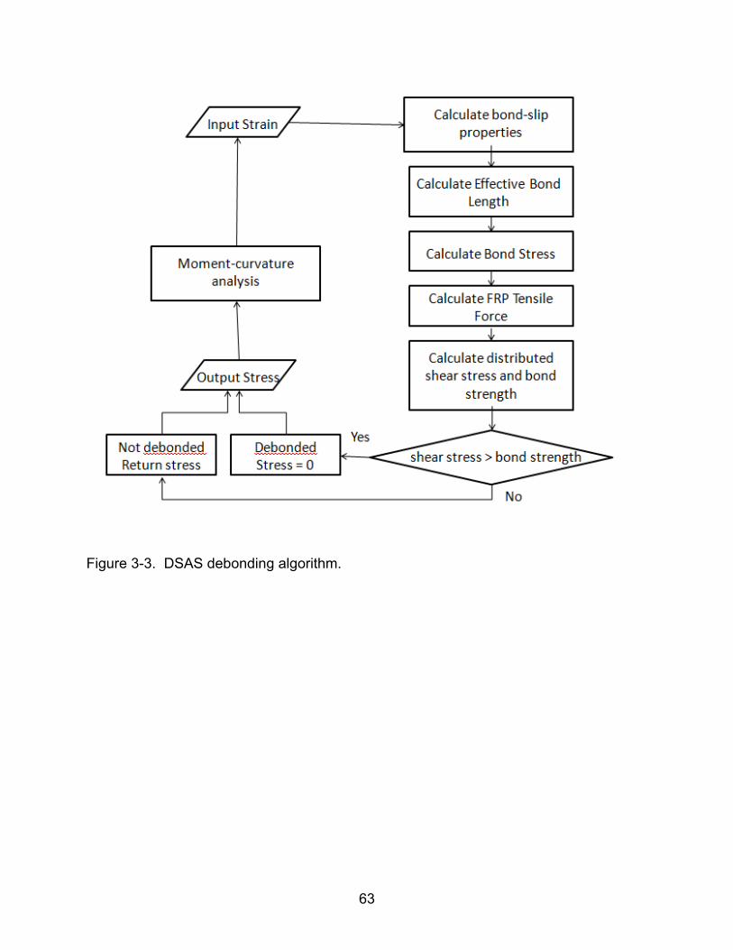
Figure 3-3. DSAS debonding algorithm.

63

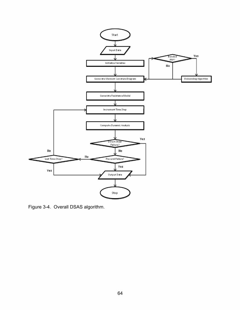
Figure 3-4. Overall DSAS algorithm.

64

CHAPTER 4 ANALYSIS

The objective of the validation of the research is to confirm the methodology

presented in Chapter 3. The validation of the methodology was conducted by

comparing results obtained from the DSAS analysis and compared to experimental test

results performed under Ross et al. (1994). The first step was to the validation of the

material model followed by the validation of the debonding process. Once the

debonding process was evaluated, the debonding process was analyzed utilizing

dynamic loading cases. Further analysis was conducted to determine if the algorithm

accounted for expected performance changes associated with the FRP’s strength,

modulus of elasticity, thickness of the layer, and the width of the FRP layer.

Material Model Validation

The material models used were based on established DSAS models. The

concrete material is based on the Modified Hognestad Parabola discussed in Chapter 2.

The steel model was based on the three stage hardening model outlined in Chapter 2.

The material properties defined by the experiment are included in Table 4-1. DSAS

input values beyond those in the experiment are included in Table 4-2. Verification of

the modified code for DSAS was completed by comparing the values for the

unretrofitted beam with the existing DSAS version 3.2.1. The inclusion of the FRP

module was found not to affect the current version of the program as the same test

results were obtained for both the existing version and the modified version. Figure 4‒1

compares the material model from the experiments conducted by Ross et al. (1994)

with those computed in DSAS. The load-displacement plot of the DSAS model closely

follows that of the experiment under four point loading. The peak displacements and

65

forces are captured in Table 4-3. The difference between the two peak displacements

is slightly over ten percent at the point of failure. The DSAS model fails earlier than the

experimental value. This could be attributed to the strain values associated with the

reinforcing steel. There was no information provided on the failure strain of the steel.

Therefore, the value used in the DSAS program could have been underestimated which

in turn would have led to the premature failure of the member and does not have an

impact on the program’s analysis. Therefore, the DSAS material model is able to

accurately capture the behavior of reinforced concrete beams under static loading case.

Debonding Validation

The debonding validation was carried out using the experimental results from

Ross et al. (1994). The experimental test produced debonding between the epoxy –

FRP interface which is contrary to the primary assumption that debonding will occur in

the concrete cover. However, the model was set up to account for that variable as long

as the bond strength of the epoxy was known. It cannot predict if debonding will occur

in the epoxy layer prior to the actual failure of the bond.

The comparison of the DSAS model and the experimental data can be viewed in

Figure 4‒2. The comparison of the load-displacement graphs indicated that the DSAS

debonding model closely followed the path of the experimental values. However, the

DSAS model failed to yield at the same point as the Experimental values. It continued

to see an increase in strength prior to the debonding of the FRP layer. Furthermore, the

experimental value had a quick drop-off from the peak load where as the DSAS model

declined from the peak value along a more gradual incline. However, the difference

between the two values is less than ten percent and is included in Table 4-4.

66

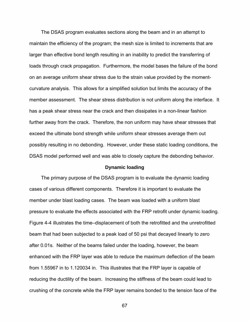
The DSAS program evaluates sections along the beam and in an attempt to

maintain the efficiency of the program; the mesh size is limited to increments that are

larger than effective bond length resulting in an inability to predict the transferring of

loads through crack propagation. Furthermore, the model bases the failure of the bond

on an average uniform shear stress due to the strain value provided by the moment-

curvature analysis. This allows for a simplified solution but limits the accuracy of the

member assessment. The shear stress distribution is not uniform along the interface. It

has a peak shear stress near the crack and then dissipates in a non-linear fashion

further away from the crack. Therefore, the non uniform may have shear stresses that

exceed the ultimate bond strength while uniform shear stresses average them out

possibly resulting in no debonding. However, under these static loading conditions, the

DSAS model performed well and was able to closely capture the debonding behavior.

Dynamic loading

The primary purpose of the DSAS program is to evaluate the dynamic loading

cases of various different components. Therefore it is important to evaluate the

member under blast loading cases. The beam was loaded with a uniform blast

pressure to evaluate the effects associated with the FRP retrofit under dynamic loading.

Figure 4-4 illustrates the time‒displacement of both the retrofitted and the unretrofitted

beam that had been subjected to a peak load of 50 psi that decayed linearly to zero

after 0.01s. Neither of the beams failed under the loading, however, the beam

enhanced with the FRP layer was able to reduce the maximum deflection of the beam

from 1.55967 in to 1.120034 in. This illustrates that the FRP layer is capable of

reducing the ductility of the beam. Increasing the stiffness of the beam could lead to

crushing of the concrete while the FRP layer remains bonded to the tension face of the

67

beam. After the concrete crushes, the beam is subjected to a greater risk of brittle

failure if the FRP ruptures or debonds from the tension face.

The use of pressure-impulse diagrams allows for the development of a failure

envelop that simplifies the assessment of a structure under various loading cases.

Figure 4-5 illustrates a pressure-impulse diagram demonstrating the ultimate failure

criteria for both cases. The beam with the FRP was able to sustain greater loading

conditions that the unretrofitted beam. Under quasi-static loading conditions, the FRP

retrofitted beam was able to withstand conditions nearly double that of the

unstrengthened member. However, the difference in resistance was much less under

the impulsive regime. This is due to the loading occurring for a short duration with the

load often being removed before the member undergoes any significant deformation.

The behavior of the beam is then determined by its natural frequency and damping.

Moreover, the loading in the impulsive regime has a greater chance of developing direct

shear failure of which FRP has minimal resistance against.

Parametric Study

The following sections discuss the various aspects associated with the behavior of

the FRP layer and its effects on the debonding behavior. The input for the parametric

study can be found in Table 4-5. This study will focus on the effect of the ultimate

strength, the elastic modulus, the thickness and the width of the reinforcing strip. There

are a wide range of FRP materials and cover a wide range of material property

combinations. This study only served to identify key components and isolate them for

the purpose of identifying their effect on the bond behavior.

68

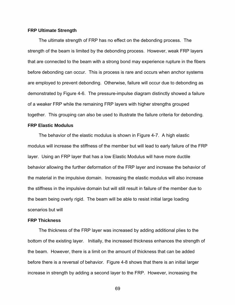
FRP Ultimate Strength

The ultimate strength of FRP has no effect on the debonding process. The

strength of the beam is limited by the debonding process. However, weak FRP layers

that are connected to the beam with a strong bond may experience rupture in the fibers

before debonding can occur. This is process is rare and occurs when anchor systems

are employed to prevent debonding. Otherwise, failure will occur due to debonding as

demonstrated by Figure 4-6. The pressure-impulse diagram distinctly showed a failure

of a weaker FRP while the remaining FRP layers with higher strengths grouped

together. This grouping can also be used to illustrate the failure criteria for debonding.

FRP Elastic Modulus

The behavior of the elastic modulus is shown in Figure 4-7. A high elastic

modulus will increase the stiffness of the member but will lead to early failure of the FRP

layer. Using an FRP layer that has a low Elastic Modulus will have more ductile

behavior allowing the further deformation of the FRP layer and increase the behavior of

the material in the impulsive domain. Increasing the elastic modulus will also increase

the stiffness in the impulsive domain but will still result in failure of the member due to

the beam being overly rigid. The beam will be able to resist initial large loading

scenarios but will

FRP Thickness

The thickness of the FRP layer was increased by adding additional plies to the

bottom of the existing layer. Initially, the increased thickness enhances the strength of

the beam. However, there is a limit on the amount of thickness that can be added

before there is a reversal of behavior. Figure 4-8 shows that there is an initial larger

increase in strength by adding a second layer to the FRP. However, increasing the

69

number of layers further limits the advantage provided by the excess material and would

not be a cost beneficial. In addition, increasing the number of layers will increase the

stiffness of the FRP strip resulting in greater shear forces along the interface leading to

possible debonding of the layers. The pressure-impulse diagram showed the thickness

peaking at 0.0350 in. The subsequent layer resulted in a small reversal suggesting that

the peak thickness would be close to 0.0350in. The last thickness was four times the

original thickness and produced a composite strength much less than the thinnest layer.

FRP Width

The width of the FRP layer had the greatest impact on the stiffness of the beam.

Increasing the width provided the best results for enhancing the strength of beam. This

is directly attributed to the greater dispersion of the interfacial shear stresses that result

in debonding. In addition to reducing the shear concentration, the increased area

provides greater tensile strength to the beam. Figure 4-9 illustrates differences

between the strips.

70

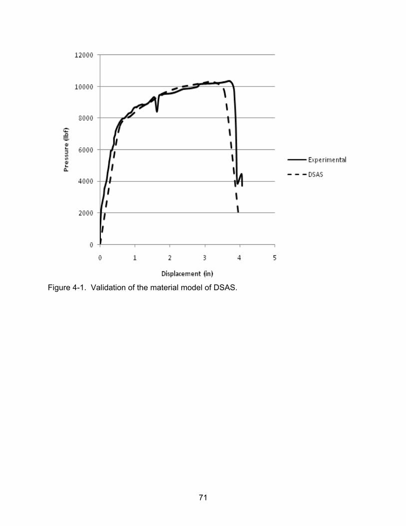
Figure 4-1. Validation of the material model of DSAS.

71

Figure 4-2. Load-displacement curve for validation of the debonding model in DSAS.

72

Figure 4-3. Moment-curvature model for validation of the debonding model in DSAS.

Figure 4-4. Time-displacement response to blast loading case.

73

Figure 4-5. Pressure-impulse curve under uniform blast loading.

74

Figure 4-6. Effect of FRP Yield Strength.

75

Figure4-7. Effect of FRP Modulus of Elasticity.

76

Figure 4-8. Effect of FRP thickness.

77

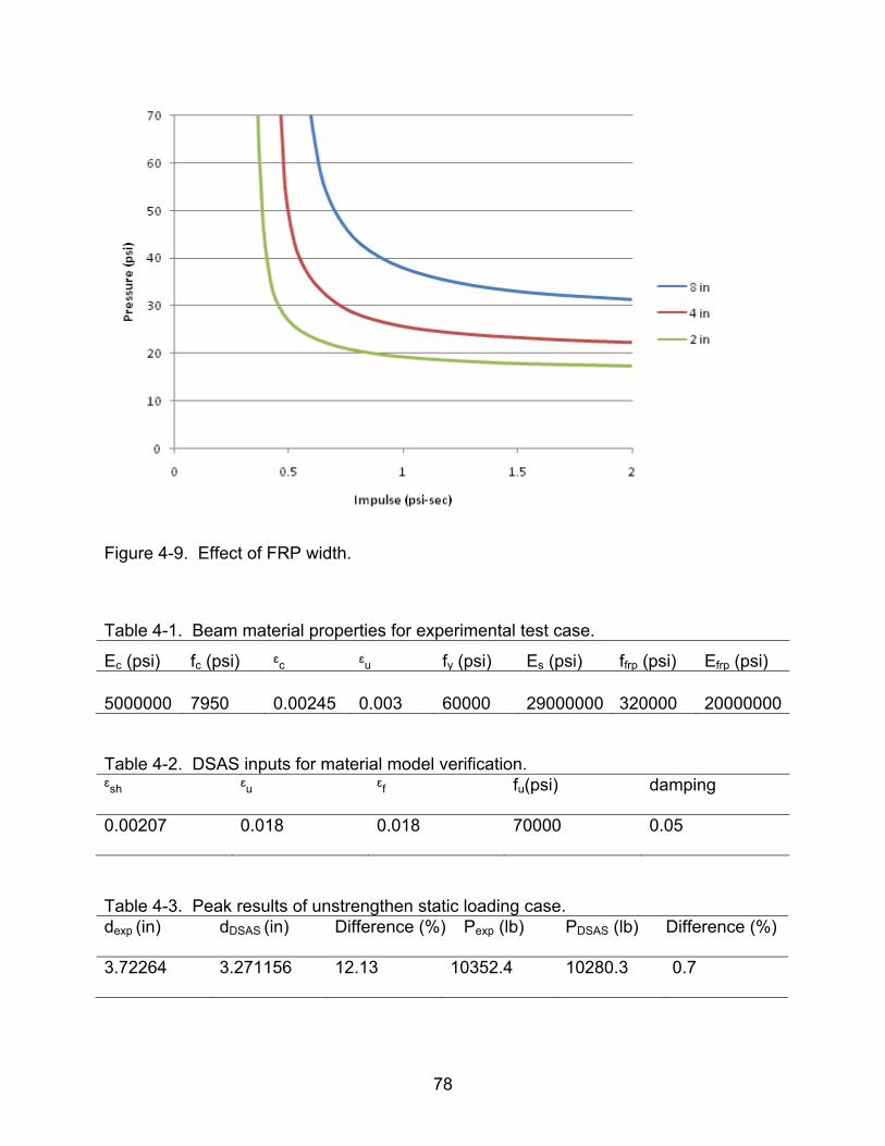
Figure 4-9. Effect of FRP width.

Table 4-1. Beam material properties for experimental test case.

Ec (psi) fc (psi) ᵋc ᵋu fy (psi) Es (psi) ffrp (psi) Efrp (psi)

5000000 7950 0.00245 0.003 60000 29000000 320000 20000000

Table 4-2. DSAS inputs for material model verification. ᵋsh ᵋu ᵋf fu(psi) damping

0.00207 0.018 0.018 70000 0.05

Table 4-3. Peak results of unstrengthen static loading case. dexp (in) dDSAS (in) Difference (%) Pexp (lb) PDSAS (lb) Difference (%)

3.72264 3.271156 12.13 10352.4 10280.3 0.7

78

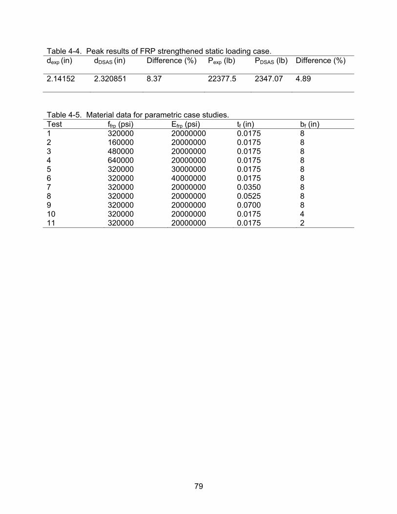
Table 4-4. Peak results of FRP strengthened static loading case. dexp (in) dDSAS (in) Difference (%) Pexp (lb) PDSAS (lb) Difference (%)

2.14152 2.320851 8.37 22377.5 2347.07 4.89

Table 4-5. Material data for parametric case studies. Test ffrp (psi) Efrp (psi) tf (in) bf (in) 1 320000 20000000 0.0175 8 2 160000 20000000 0.0175 8 3 480000 20000000 0.0175 8 4 640000 20000000 0.0175 8 5 320000 30000000 0.0175 8 6 320000 40000000 0.0175 8 7 320000 20000000 0.0350 8 8 320000 20000000 0.0525 8 9 320000 20000000 0.0700 8 10 320000 20000000 0.0175 4 11 320000 20000000 0.0175 2

79

CHAPTER 5 SUMMARY AND CONCLUSIONS

This chapter outlines the various observations made as part of the validation for

the debonding behavior as it pertains to the modification of the DSAS program. The

limitations observed as part of the analysis will be address as well as recommendations

and future research opportunities for the further development of the retrofit model.

Limitations

Various limitations were encountered during the validation process of this study.

The results are based primarily on experimental static loading cases and as there are

limited severe dynamic loading cases associated with beams information to perform

adequate comparisons to validate the dynamic behavior of the debonding model in

DSAS. Previous dynamic enhancement factors are addressed in Chapter 2, but a lack

of experimental dynamic tests limited the ability to evaluate if high strain rates in the

epoxy and the FRP layers have a significant impact on the debonding behavior when

compared to steel and concrete. However, since most debonding behavior occurs in

concrete, it may not be possible to accurately separate strain rates associated with the

FRP and epoxy from the concrete.

Most models for bending incorporate a mixed mode of failure. DSAS currently

lacks the ability to properly evaluate the effects of discontinuities in the displacement

due to flexural cracks that may result in peeling effects. Therefore, the DSAS

debonding module is limited to the evaluation of debonding based solely on the

interfacial shear. While the deviations will be minimal under pure bending cases with

uniform loading, it will limit that programs ability to accurately predict the behavior of

more severe loading cases. Both close proximity blast loading and impact loading will

80

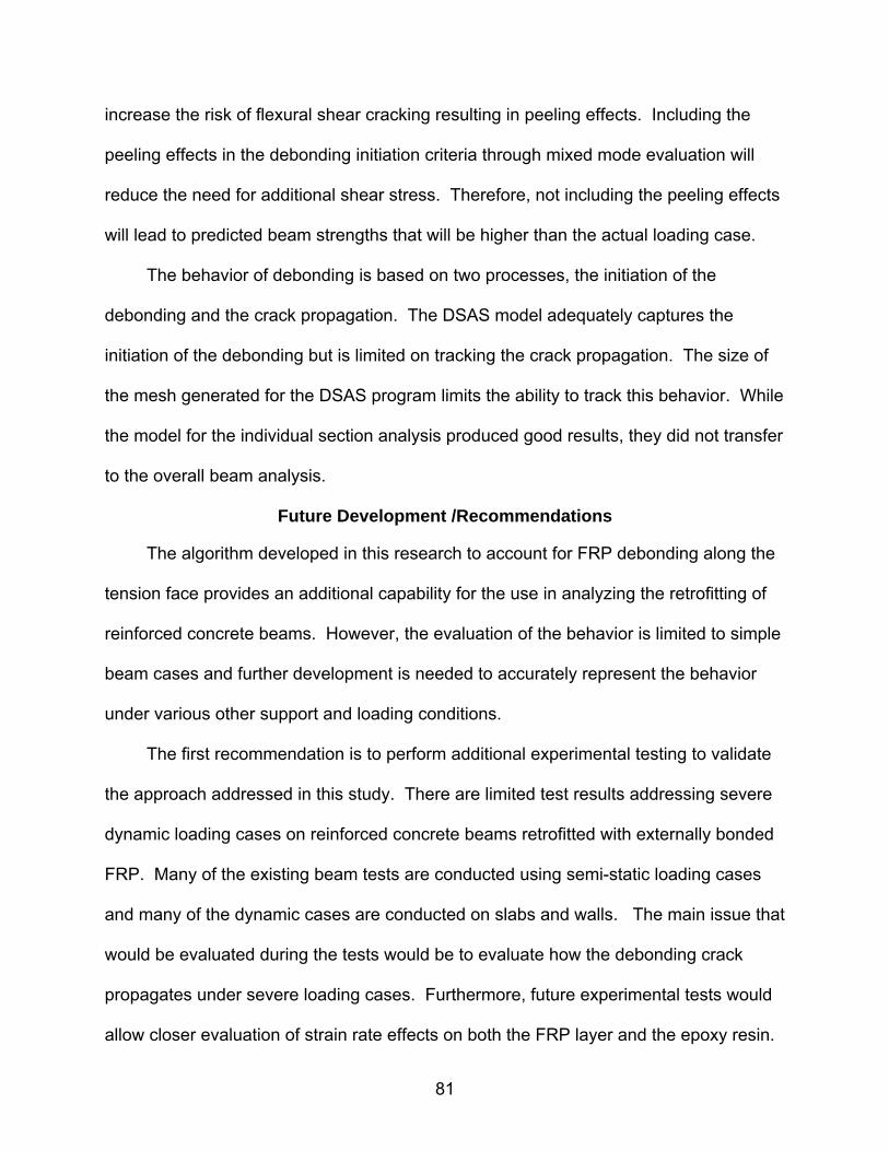
increase the risk of flexural shear cracking resulting in peeling effects. Including the

peeling effects in the debonding initiation criteria through mixed mode evaluation will

reduce the need for additional shear stress. Therefore, not including the peeling effects

will lead to predicted beam strengths that will be higher than the actual loading case.

The behavior of debonding is based on two processes, the initiation of the

debonding and the crack propagation. The DSAS model adequately captures the

initiation of the debonding but is limited on tracking the crack propagation. The size of

the mesh generated for the DSAS program limits the ability to track this behavior. While

the model for the individual section analysis produced good results, they did not transfer

to the overall beam analysis.

Future Development /Recommendations

The algorithm developed in this research to account for FRP debonding along the

tension face provides an additional capability for the use in analyzing the retrofitting of

reinforced concrete beams. However, the evaluation of the behavior is limited to simple

beam cases and further development is needed to accurately represent the behavior

under various other support and loading conditions.

The first recommendation is to perform additional experimental testing to validate

the approach addressed in this study. There are limited test results addressing severe

dynamic loading cases on reinforced concrete beams retrofitted with externally bonded

FRP. Many of the existing beam tests are conducted using semi-static loading cases

and many of the dynamic cases are conducted on slabs and walls. The main issue that

would be evaluated during the tests would be to evaluate how the debonding crack

propagates under severe loading cases. Furthermore, future experimental tests would

allow closer evaluation of strain rate effects on both the FRP layer and the epoxy resin.

81

The second recommendation is to expand the debonding model out to account for

fixed end support beams. The used of fixed end supports will cause negative moment

situations at the supports that could lead to buckling of the FRP strips forcing premature

debonding at the ends and reducing the capacity. Hardened epoxy has small

compression strength and acts as a solid element. Even if the tension on the FRP layer

is not enough to initiate fracture damage due to shear stresses along the interface, a

buckling action could result in a peeling effect initiating crack propagation starting at the

end of the beam and progressing inward.

The third recommendation is to include the addition of an anchor system in the

FRP reinforcing layer. The first issue will account for the inclusion of anchors along the

supports. The used of anchors along the supports will allow for the development of a

tension membrane. This will allow the increased enhancement of the member even

after the FRP debonds from the face of the concrete. Furthermore, the inclusion of

anchors along the edges will force debonding to initiate in the center of the member

compared to at the plate ends under normal bonding conditions. The second issue will

account for the inclusion of an anchoring system along the face of the beam. The

bonded region will only sustain up to an ultimate strength defined by the effective bond

length. If the shear stresses along the interfaces exceed that amount, the debonding

crack will continue to propagate until either the shear stresses are less than the ultimate

strength or the FRP completely debonds from the bottom of the beam. The inclusion of

anchors along the base of the beam will limit the ability for the crack to propagate

beyond a given distance and will prevent total failure of the FRP layer. Future research

should evaluate the types of anchors and the placement of the anchors.

82

The final recommendation is to research the effectiveness of FRP when applied as

shear reinforcement. The use of FRP along the tension face is effective at increasing

the strength of the member in flexure. However, the development of flexural shear

cracks will allow for debonding to occur at lesser loading cases. Applying exterior

bonded FRP along the shear plain could reduce the size of the diagonal cracking in the

member. Furthermore, wrapping the FRP up the sides of the beam will add increased

anchor strength by increasing the bonded area that needs to fail in order for debonding

to initiate and propagate along the tension face.

General Conclusions

A new assessment module was developed for DSAS to address the strengthening

of reinforced concrete members with FRP on the tension face. The inclusion of this

module has the ability to enhance the capability of the program to analyze members

that have been subjected to FRP retrofits. Further research is required to accurately

capture the behavior of retrofits under different load cases and boundary supports. The

current model is capable of capturing the debonding behavior based solely on the

interfacial shear which is suitable for beams that do not experience any discontinuities

due to flexural shear cracks.

This study has shown that the inclusion of FRP along the tension face has the

ability to initially increase the strength of the member. The FRP provides the beam the

ability to sustain higher loads and reduces the maximum displacement. However, the

strength increase is limited by the bond strength at the FRP-concrete interface.

Furthermore, employment of FRP over reinforces the members and increases the

possibility of concrete crushing along the compression face. Failure of the FRP, either

83

84

by debonding or rupture, after the concrete is damaged could result in brittle failure of

the member.

The choice of FRP and its properties will determine the behavior of the beam.

Overly stiff members will suitable under quasi-static loading. However, these members

perform poorly under impulsive loading. Therefore, under impulsive loading, the use of

less rigid FRP reinforcement should be employed to enhance the performance of the

beam under dynamic loading.

REFERENCE LIST

ABAQUS (2010). ABAQUS Version 6.10 documentation. Dasault Systemes, Simulia Corp, Providence, RI, USA.

Aiello, M.A., Leone, M. (2008). “Interface analysis between FRP EBR system and

concrete.” Composites, Part B: Engineering, 39, 618-626. American Concrete Institute (2008). Building Code Requirement for Structural Concrete

(ACI 318-08) and Commentary. Bank, L.C., Borowicz, D.T., Arora, D., Lamanna, A.J., Velazauez, G.I., Ray, J.C. (2004).

“Strengthening of concrete beams with fasteners and composite material strips-scaling and anchorage issues.” Technical Report ERDC/GSL TR-04-5, U.S. Army Engineer Research and Development Center, Vicksburg, MS.

Biggs, J.M. (1964). Introduction to structural dynamics. McGraw-Hill Book Company,

New York, NY. Blasko, J.R., Krauthammer, T., Astarlioglu, S. (2007). “Pressure-impulse diagrams for

structural elements subjected to dynamic loads.” Technical report PTC-TR-002-2007, Protective Technology Center, The Pennsylvania State University, PA.

Buchan, P.A., Chen, J.F. (2007). “Blast resistance of FRP composites and polymer

strengthened concrete and masonry structures – A state-of-the-art review.” Composites, Part B: Engineering, 38( 5-6), 509-522.

Buyle-Bodin, F., David, E., Ragneau, E. (2002). “Finite element modeling of flexural

behavior of externally bonded CFRP reinforced concrete structures.” Engineering Structures, 24(11), 1423-1429.

Chee, K.H., Krauthammer, T., Astarlioglu, S. (2008). “Analysis of shallow buried

reinforced concrete box structures subjected to air blast loads.” Rep No. CIPPS-TR-002-2008. Center for Infrastructure Protection and Physical Security, University of Florida, FL.

Chen, J.F., Teng, J.G. (2001). “Anchorage strength models for FRP and steel plates

bonded to concrete.” Journal of Structural Engineering, ASCE, 127( 7), 784-791. GangaRao, H.V.S., Taly, N., Vijay, P.V. (2007). Reinforced concrete design with FRP

composites. CRC Press, Boca Raton, FL. Hawkins, N.M. (1974). “The strength of stud shear connections.” Civil Engineering

Transactions, IE, Australia, 29-45. Hsu, T. T. (1993). Unified Theory of Reinforced Concrete. CRC Press.

85

Hutchinson, J.W., Suo, Z. (1991). “Mixed mode cracking in layered materials.” Advances in Applied Mechanics, Elsevier, 29, 63-191.

Johnson, R., Saiidi, M., Maragakis, M. (2005). “A study of fiber reinforced plastics for

seismic bridge restrainers.” Report No. CCEER-05-02. Center of Civil Engineering Earthquake Research, Department of Civil Engineering, University of Nevada, Reno, Nevada.

Kachlakev, D., McCurry, D.D. (2000). “Behavior of full-scale reinforced concrete beams

retrofitted for shear and flexural with FRP laminates.” Composites, Part B: Engineering, 31(6-7), 445-452.

Krauthammer, T. (1984). “Shallow-buried RC box type structures.” Journal of Structural

Engineering, ASCE, 110( 3), 637-651. Krauthammer, T. (2008). Modern Protective Structures. CRC Press, Boca Raton, FL. Krauthammer, T., Bazeos, N., Holmquist, T.J. (1986). “Modified SDOF Analysis of R. C.

Box-Type Structures.” Journal of Structural Engineering, 112(4), 726-744. Krauthammer, T., Frye, M.T., Schoedel, R., Seltzer, M., Astariolgu, S. (2003). “A Single-

Degree-of-Freedom (SDOF) Computer Code Development for the Analysis of Structures Subjected to Short-Duration Dynamic Loads.” Technical Report PTC-TR-002-2003. Protective Technology Center, The Pennsylvania State University.

Krauthammer, T., Schoedel, R., Shanaa, H. (2002). “An Analysis Procedure for Shear in

Structural Concrete Members Subjected to Blast”. Technical report PTC-TR-001-2002, Protective Technology Center, The Pennsylvania State University, PA.

Krauthammer, T., Shahriar, S. (1988). “A Computational Method for Evaluating Modular

Prefabricated Structural Element for Rapid Construction of Facilities, Barriers, and Revetments to Resist Modern Conventional Weapons Effects.” Report ESL-TR-87-60, Engineering & Services Laboratory Air Force Engineering & Services Center, Tyndall Air Force Base, Florida.

Li, L.J.,Guo, Y.C., Huang, P.Y., Liu, F., Deng, J., Zhu, J. (2009).”Interfacial stress

analysis of RC beams strengthened with hybrid CFS and GFS.” Construction and Building Materials, 23, 2394-2401.

Lu, X.Z., Teng, J.G., Ye, L.P., Jiang, J.J. (2005). “Bond-slip models for FRP

sheets/plates bonded to concrete.” Engineering Structures, 27( 6), 920-937. Maalej, M., Leong, K.S. (2005). “Effect of beam size and FRP thickness on interfacial

shear stress concentration and failure mode of FRP-strengthened beams.” Composites Science and Technology, 65( 7-8), 1148-1158.

86

MacGregor, G.J., Wight K.J. (2009). Reinforced Concrete: Mechanics and Design. Pearson Prentice Hall, New Jersey.

Morency, D., Krauthammer, T., Astarlioglu, S. (2010). “Large deflection behavior effect

in reinforced concrete column under severe dynamic short duration load.” Report CIPPS-TR-001-2010. Center for Infrastructure Protection and Physical Security, University of Florida, FL.

Newmark, N.M., IABSE, M., ASCE, F. (1962). “A Method of Computation for Structural

Dynamics.” American Society of Civil Engineers, Paper, 127(3384), 601-630. Pan, J., Leung, C.K.Y. (2007). “Debonding along the FRP-concrete interface under

combined pulling/peeling effects.” Engineering Fracture Mechanics, 74(1-2), 132-150.

Park, R., Gamble, W.L. (2000). Reinforced Concrete Slabs. John Wiley & Sons, Inc.

New-York, NY. Park, R., and Paulay, T. (1975). Reinforced concrete structures. Wiley. Pham, H., Al-Mahaidi, R. (2004). “Experimental investigation into flexural retrofitting of

reinforced concrete bridge beams using FRP composites.” Composite Structures, 66(1-4), 617-625.

Razaqpur, A.G., Tolba, A., Contestabile, E. (2007). “Blast loading response of

reinforced concrete panels reinforced with externally bonded GFRP laminates.” Composites, Part B: Engineering, 38(5-6), 535-546.

Ross, C.A., Jerome, D.M., Hughes, M.L. (1994). “Hardening and rehabilitation of

concrete structures using carbon fiber reinforced plastics (CFRP).” Report WL-TR-94-7100, Wright Laboratory, Armament Directorate, Elgin AFB, FL.

Ross, C.A, Kuennen, S.T., Strickland, W.S. (1989). “High strain rate effects on tensile

strength of concrete.”Fourth International Symposium on the Interaction of Non-nuclear Munitions with Structures, (1989) Panama City Beach, FL.

Rougier, V.C., Luccioni, B.M. (2007). “Numerical assessment of FRP retrofitting

systems for reinforced concrete elements.” Engineering Structures, 29(8), 1664-1675.

Shanaa, M.H. (1991). “Response of Reinforced Concrete Structural Elements to Severe

Impulsive Loads.” Protective Technology Center, The Pennsylvania State University, PA.

87

88

Silva, P.F., Lu, B. (2007).”Improving the blast resistance capacity of RC slabs with innovative composite materials.” Composites, Part B: Engineering, 38(5-6), 523-534.

Slawson, T.R. (1984). “Dynamic Shear Failure of Shallow-Burried Flat-Roofed

Reinforced Concrete Structures Subjected to Blast Loading.” U.S. Army Engineer Waterways Experimental Station, April.

Smith, S.T., Hu, S., Kim, S.J., Seracino, R. (2011). “FRP-strengthened RC slabs

anchored with FRP anchors.” Engineering Structures, 33(4), 1075-1087. Soroushian, P., Obaseki, K. (1986). “Strain Rated-Dependent Interaction Diagrams for

Reinforced Concrete Section.” American Concrete Institute Journal. 83(1), 108-116.

Sozen, M.A. (1974). “Hysteresis in Structural Elements.” Applied Mechanics in

Earthquake Engineering. Applied Mechanics Division , ASME, 8, 63 – 98. Tedesco, J.W., McDougal, W.G. and Ross, C.A. (1999). Structural Dynamics: Theory

and Applications. Addison-Wesley Longman Inc: Menlo Park, CA. Teng, J.G., Smith, S.T., Yao, J., Chen, J.F. (2003). “Intermediate crack-induced

debonding in RC beams and slabs.” Construction and Building Materials, 17(6-7), 447-462.

Tran, P.T., Krauthammer, T., Astarlioglu, S. (2009). “Effect of short-duration-high-

impulse variable axial and transverse loads on reinforced concrete column.” Report CIPPS-TR-001-2009. Center for Infrastructure Protection and Physical Security, University of Florida, FL.

Wang, J., Zhang, C. (2008). “Nonlinear fracture mechanics of flexural-shear crack

induced debonding of FRP strengthened concrete beams.” International Journal of Solids and Structures, 45(10), 2916-2936.

Yuan, H., Teng, J.G., Seracino, R., Wu, Z.S., Yao, J. (2004). “Full-range behavior of

FRP-to-concrete bonded joints.” Engineering Structures, 26(5), 553-565.

BIOGRAPHICAL SKETCH

Graham Long was born in The Pas, Manitoba, Canada. In 2000, he joined the

Canadian Forces and attended the Royal Military College of Canada under a military

sponsored officer program.

Upon graduation in May 2004, he earned his Bachelor of Engineering degree in

Civil Engineering and obtained his officer’s commission and begun serving as a military

engineer. In 2006, he was deployed to Afghanistan as a part of a construction

engineering support unit. Upon his return, he was posted to Canadian Forces Base

Suffield as a member of the base infrastructure engineering branch. In 2010, he was

awarded a postgraduate scholarship from the Canadian Forces to pursue a master’s

degree in civil engineering at the University of Florida, specializing in the field of

protective structures.

Upon completion of his master’s program, Graham will be assigned to the

Engineering Support Unit in Moncton, New Brunswick, Canada.

89