1

JUAS 2019 – NORMAL CONDUCTING MAGNETS – TUTORIAL

18. – 20. FEB. 2019

CASE STUDY - TUTORIAL

NUMERICAL DESIGN OF A NORMAL-CONDUCTING, IRON-DOMINATED ELECTRO-MAGNET USING FEMM 4.21

Th. Zickler, CERN, 2019

1. INTRODUCTION

Finite Element Method Magnetics (FEMM) written by David Meeker is a finite element

package for solving 2D planar and axisymmetric problems in low frequency magnetics and

electrostatics. It is powerful and simple and therefore makes and excellent starting point for

learning FEA. The program runs under Windows. The program can be obtained via the FEMM

home page at http://www.femm.info/wiki/HomePage. The package is composed of an

interactive shell encompassing graphical pre- and post-processing, a mesh generator, and

various solvers. A powerful scripting language, Lua 4.0, is integrated with the program. Lua

allows users to create batch runs, describe geometries parametrically, perform optimizations,

etc. Lua is also integrated into every edit box in the program so that formulas can be entered

instead of numerical values, if desired (detailed information on Lua is available from

http://www.lua.org). There is no hard limit on problem size - maximum problem size is limited

by the amount of available memory.

The purpose of this document is to present a step-by-step tutorial to help the students get "up

and running" with FEMM. In this document, the solution for the normal-conducting, iron

dominated electro-magnet is considered.

1 This text is based on the original tutorial written by David Meeker

2

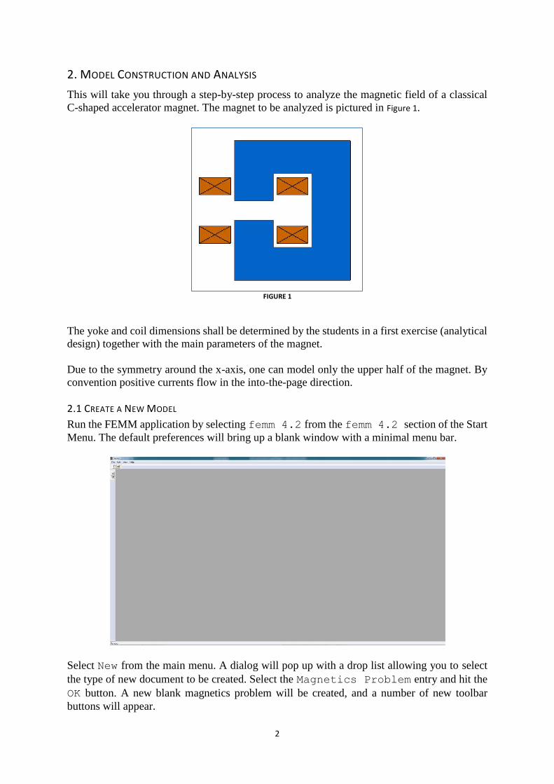
2. MODEL CONSTRUCTION AND ANALYSIS

This will take you through a step-by-step process to analyze the magnetic field of a classical

C-shaped accelerator magnet. The magnet to be analyzed is pictured in Figure 1.

FIGURE 1

The yoke and coil dimensions shall be determined by the students in a first exercise (analytical

design) together with the main parameters of the magnet.

Due to the symmetry around the x-axis, one can model only the upper half of the magnet. By

convention positive currents flow in the into-the-page direction.

2.1 CREATE A NEW MODEL

Run the FEMM application by selecting femm 4.2 from the femm 4.2 section of the Start

Menu. The default preferences will bring up a blank window with a minimal menu bar.

Select New from the main menu. A dialog will pop up with a drop list allowing you to select

the type of new document to be created. Select the Magnetics Problem entry and hit the

OK button. A new blank magnetics problem will be created, and a number of new toolbar

buttons will appear.

3

2.2 SET PROBLEM DEFINITION

The first task is to tell the program what sort of problem is to be solved. To do this, select

Problem from the main menu. The Problem Definition dialog will appear. Set

Problem Type to Planar. Make sure that Length Units is set to Millimetres and

that the Frequency is set to 0. At this stage, also the length of the model can be entered by

using the Depth field. When the proper values have been entered, hit the OK button.

We can adjust the view so that it will contain the entire solution region. Select

View|Keyboard from the main menu to bring up a dialog that allows you to specify the

extents of the visible screen. When ready hit the OK button and the screen will then be rescaled

to the smallest rectangle that contains the specified region.

4

2.3 DRAW BOUNDARIES

The first task is to draw boundaries for the solution region. Fundamentally, finite element

solvers mesh and find a solution over a finite region of space that contains the objects of

interest. In this case, we will choose our solution region to be a rectangle extending about 2

times the dimension of the magnet yoke in the directions left, right and upwards (Note that the

horizontal center line (=x-axis) is the symmetry axis which is already a boundary line for the

solution region).

First, node points need to be defined that bound the rectangle. To draw these node points, select

the Operate on nodes button from the tool bar (this is the farthest button on the left with

a small black box). Place the four nodes on the plane either by moving the mouse pointer to

the desired location and pressing the left mouse button, or by pressing the <TAB> key and

manually entering the point coordinates via a popup dialog.

Select the Operate on segments toolbar button (second button from the left with a blue

line). To select a node to be the endpoint of a line, click near the desired endpoint with the left

mouse button. Draw a line by selecting the second node; a line will appear linking the nodes

as soon as the second point is selected. Continue in this way with the other points until the

rectangle is complete.

Instead of straight line, one can also draw arcs. In this case select the Operate on arc

segments toolbar button (third button from the left with a blue arc). Draw an arc by selecting

two points. After the second point has been selected a dialog will appear asking you for some

attributes of the arc. In FEMM, arcs are approximated by a series of small, straight lines. The

Max. segment specifies the coarseness with which the arc is divided into sections.

2.4 DRAW COIL AND IRON YOKE

Now, the coils and the iron yoke can be drawn. Switch back to Nodes mode by pressing the

Operate on nodes toolbar button. For each region, place nodes defining the extents of

the region. Select the Operate on segments toolbar button so that lines can be drawn

connecting the points. By selecting the nodes defining the region in sequence, one obtains lines

between each of the nodes. Repeat this operation until all regions are defined.

5

2.5 PLACE BLOCK LABELS

Now click on the Operate on Block Labels toolbar button denoted by concentric green

circles. Place a block label in the each of the regions (don’t forget the air region outside the

yoke region). Like node points, block labels can be placed either by a click on the left mouse

button, or via the <TAB> dialog. The program uses block labels to associate materials and

other properties with various regions in the problem geometry. Next, we will define some

material properties, and then we will go back and associate them with particular block labels.

6

2.6 ADD MATERIALS TO THE MODEL

Select Properties|Materials Library from the main menu. Then drag-and-drop Air

from Library Materials to Model Materials to add it to the current model. Go into

the Solid Non-Magnetic Conductors folder and drag Copper into Model

Materials. As yoke material choose Cold rolled low carbon strip steel in

folder Metals Handbook DC Magnetization Curves. Click on OK.

The properties of selected materials a sufficiently defined now. However, if you want to change

them you can do this by clicking on Properties|Materials in the main menu and

selecting the material to be changed in the pull-down list Property Name. The click on

Modify Property. We will change here the properties of the Cold rolled low

carbon strip steel.

Once the Block Property window is open select Laminated in-plane from the

Special Attributes: Lamination & Wire Type section. Set the Lam

thickness, mm to 1 and the Lam fill factor to 0.98 to take into account that the

yoke will be made of 1 mm thick steel laminations.

7

Also the magnetic properties and in particular the B-H data of the steel can be changed here.

For entering or modifying Nonlinear Material Properties press the Edit B-H

Curve button and the B-H Curve Data dialog box will open.

After you are done entering or changing your B-H data points, it is a good idea to view the B-

H curve to see that it looks like it is “supposed” to. This is done by pressing the Plot B-H

Curve button or the Log Plot B-H Curve button on the B-H data dialog. You should

see a B-H curve that looks something like the curve pictured below. The boxes in the plot

represent the locations of the entered B-H points, and the line represents a cubic spline derived

from the entered data.

8

For more information see the manual.

2.7 ADD A "CIRCUIT PROPERTY" FOR THE COIL

Select Properties|Circuits from the main menu. On the dialog that appears, push the

Add Property button to create a new circuit property. Name the circuit by replacing the

New Circuit name with Coil. Specify that the circuit property is to be applied to a wound

region by selecting the Series radio button. Enter the current value in Circuit Current.

Click on OK for both the Circuit Property and Property Definition dialogs.

2.8 ASSOCIATE PROPERTIES WITH BLOCK LABELS.

If not already activated, click on the Operate on Block Labels toolbar button. Right

click on the block label node in the air region outside the coil. The block label will turn red,

denoting that it is selected. Press space to open the selected block label (instead of pressing the

space bar, one can use the Open up Properties Dialog toolbar button). A dialog will

pop up containing the properties assigned to the selected label. Set the Block type to Air.

Uncheck the Let Triangle choose Mesh Size checkbox and enter a number for the

Mesh size. The mesh size parameter defines a constraint on the largest possible elements

size allowed in the associated section. The mesher attempts to fill the region with nearly

equilateral triangles in which the sides are approximately the same length as the specified Mesh

size parameter. When the “Let Triangle choose Mesh Size” box is checked, the mesher is

free to pick its own element size, usually resulting in a somewhat coarse mesh. Click on OK.

9

The block label will then be labeled as Air, and a circle will appear about the block label

indicating the approximate mesh size in the associated region.

Repeat the same for the block label node inside the first coil region. The Block type for the

coils has to be set to Copper. We want to assign currents to flow in this region, so select the

Coil circuit from the In Circuit drop list. The Number of turns edit box will become

activated if a series-type circuit is selected for the region (e.g. the Coil property that was

previously defined). Enter the number of turns for this region, denoting that the region if filled

turns wrapped in a counter-clockwise direction (i.e. positive turns in the right-hand-screw rule

sense). Click on OK.

Repeat the same procedure for the second coil region but set the negative sign in front of the

number of turns to define that the current direction in this coil is negative. Click on OK.

In the last operation, set the Block type for the yoke region to Cold rolled low

carbon strip steel and click on OK.

10

2.9 CREATE BOUNDARY CONDITIONS

Select Properties|Boundary from the menu bar, and then click on the Add Property

button. Replace the name New Boundary with Dirichlet and select Prescribed A

as BC Type.

With this type of boundary condition, the vector potential, A, is prescribed along a given

boundary. This boundary condition can be used to prescribe the flux passing normal to a

boundary, since the normal flux is equal to the tangential derivative of A along the boundary.

In our case we leave all parameters at zero. This means that you have just defined a Dirichlet

boundary condition with the vector potential equals zero which means zero magnetic flux

through the plane. Next you have to assign this condition to a particular part of the model (i.e.

the boundary of your background air region).

Select Lines from the toolbar then right click on the left side of the background region. When

it turns red you have selected it. Now press space bar and the Segment Property window

will appear. From the top drop box change the segment type from <None> to Dirichlet.

The Segment Property dialog boy allows you also to change the element size along the

selected line. After the line properties have been modified click on OK. Repeat this process for

the right side and the top side of the background region.

11

Note that the Neumann boundary condition (normal derivative of vector potential ∂A/∂n = 0)

is set automatically since the first-order triangle finite elements give a ∂A/∂n = 0 boundary

condition by default. Therefore, no specific boundary condition needs to be set for the

symmetry axis (the bottom line of the background region).

2.10 GENERATE MESH AND RUN FEA

Now save the file and click on the toolbar button with yellow mesh. This action generates a

triangular mesh for your problem. If the mesh spacing seems to fine or too coarse you can

select block labels or line segments and adjust the mesh size defined in the properties of each

object. Once the mesh has been generated, click on the “turn the crank” button to analyze your

model.

Processing status information will be displayed. If the progress bars do not seem to be moving

then you should probably cancel the calculation. This can occur if insufficient boundary

conditions have been specified. For this particular problem, the calculations should be

completed within a few seconds. There is no confirmation for when the calculations are

complete; the status window just disappears when the processing is finished.

12

3. ANALYSIS RESULTS

Click on the glasses icon to view the analysis results. A post-processor window will appear.

The post-processor window will allow you to extract many different sorts of information from

the solution.

13

3.1 POINT VALUES

Just like the pre-processor, the post-processor window has a set of different editing modes:

Point, Contour, and Area. The choice of mode is specified by the mode toolbar buttons, i.e.

where the first button corresponds to Point mode, the second to Contour mode, and the third to

Area mode. By default, when the program is first installed, the post-processor starts out in Point

mode. By clicking on any point with the left mouse button, the various field properties

associated with that point are displayed in the floating FEMM Output window. Similar to

drawing points in the pre-processor, the location of a point can be precisely specified by

pressing the <TAB> button and entering the coordinates of the desired point in the dialog that

pops up.

3.2 COIL TERMINAL PROPERTIES

With FEMM, it is straightforward to determine the inductance and resistance of the coil as seen

from the coil's terminals. Press the button to display the resulting attributes of each Circuit

Property that has been defined.

Since only one half of the magnet has been modelled, the values need to be multiplied by two

get the total magnet resistance and inductance. However, the problem does not take into

account the coil heads on both ends of the magnet, so the results will be significantly lower

than on a real magnet.

14

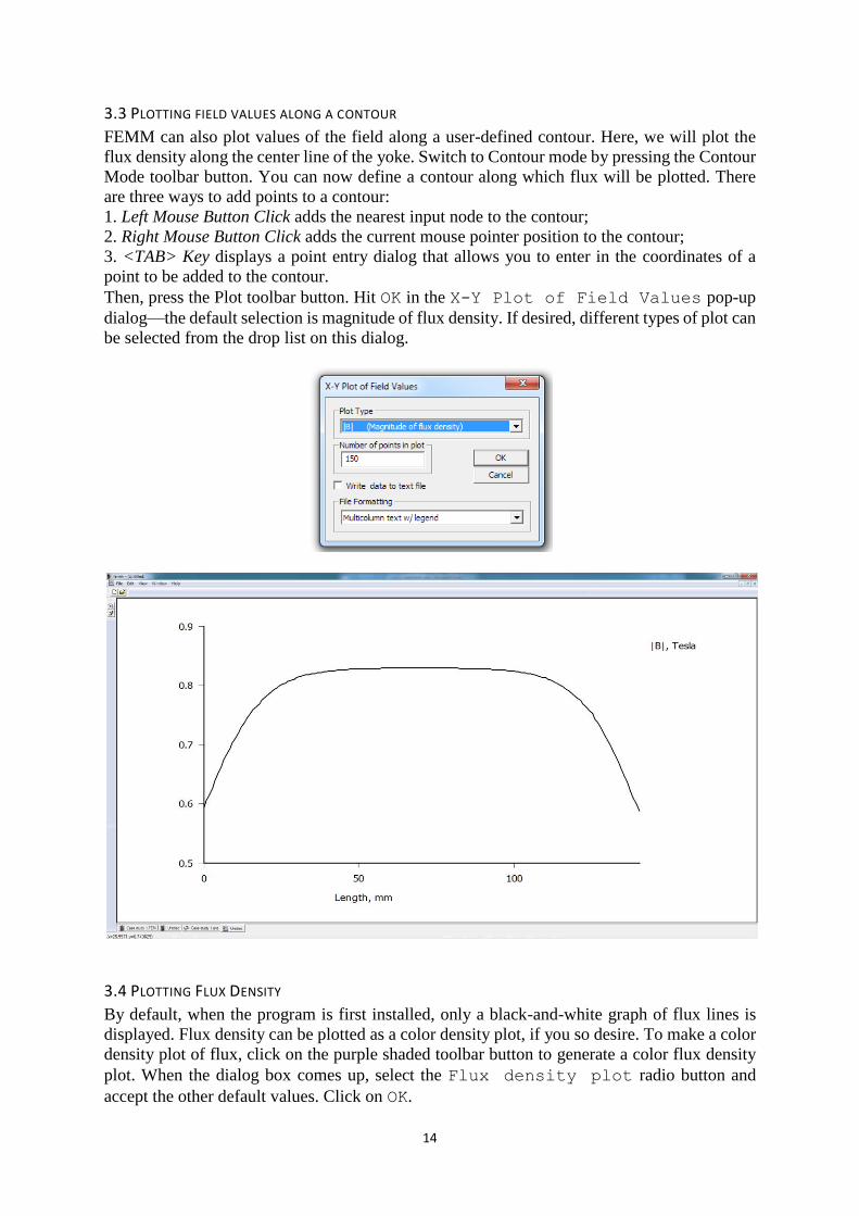
3.3 PLOTTING FIELD VALUES ALONG A CONTOUR

FEMM can also plot values of the field along a user-defined contour. Here, we will plot the

flux density along the center line of the yoke. Switch to Contour mode by pressing the Contour

Mode toolbar button. You can now define a contour along which flux will be plotted. There

are three ways to add points to a contour:

1. Left Mouse Button Click adds the nearest input node to the contour;

2. Right Mouse Button Click adds the current mouse pointer position to the contour;

3. <TAB> Key displays a point entry dialog that allows you to enter in the coordinates of a

point to be added to the contour.

Then, press the Plot toolbar button. Hit OK in the X-Y Plot of Field Values pop-up

dialog—the default selection is magnitude of flux density. If desired, different types of plot can

be selected from the drop list on this dialog.

3.4 PLOTTING FLUX DENSITY

By default, when the program is first installed, only a black-and-white graph of flux lines is

displayed. Flux density can be plotted as a color density plot, if you so desire. To make a color

density plot of flux, click on the purple shaded toolbar button to generate a color flux density

plot. When the dialog box comes up, select the Flux density plot radio button and

accept the other default values. Click on OK.

15

4. CONCLUSIONS

You have now completed your first model of a magnetic problem with FEMM. From this

basic introduction, you have been exposed to the following concepts:

How to draw a model using nodes, segments, arc, and block labels;

How to add material to your model and how to assign them to regions;

How to specify the finite element mesh size;

How to define boundary for your model;

How to define and apply boundary conditions;

How to analyse a problem;

How to inspect local field values;

How to plot field values along a line;

How to compute inductance and resistance;

How to display colour flux density plots.

Hopefully, this tutorial has provided you enough of the basics of FEMM so that you can

explore more complicated problems.