energies

Article

Numerical Investigation of AerodynamicPerformance and Loads of a Novel Dual RotorWind TurbineBehnam Moghadassian †, Aaron Rosenberg † and Anupam Sharma *

Department of Aerospace Engineering, Iowa State University, Ames, IA 50010, USA;behmogh@iastate.edu (B.M.); aaronr@iastate.edu (A.R.)* Correspondence: sharma@iastate.edu; Tel.: +1-515-294-2884† These authors contributed equally to this work.

Academic Editor: Frede BlaabjergReceived: 15 April 2016; Accepted: 6 July 2016; Published: 21 July 2016

Abstract: The objective of this paper is to numerically investigate the effects of the atmosphericboundary layer on the aerodynamic performance and loads of a novel dual-rotor wind turbine(DRWT). Large eddy simulations are carried out with the turbines operating in the atmosphericboundary layer (ABL) and in a uniform inflow. Two stability conditions corresponding to neutraland slightly stable atmospheres are investigated. The turbines are modeled using the actuator linemethod where the rotor blades are modeled as body forces. Comparisons are drawn betweenthe DRWT and a comparable conventional single-rotor wind turbine (SRWT) to assess changesin aerodynamic efficiency and loads, as well as wake mixing and momentum and kinetic energyentrainment into the turbine wake layer. The results show that the DRWT improves isolated turbineaerodynamic performance by about 5%–6%. The DRWT also enhances turbulent axial momentumentrainment by about 3.3%. The highest entrainment is observed in the neutral stability case whenthe turbulence in the ABL is moderately high. Aerodynamic loads for the DRWT, measured asout-of-plane blade root bending moment, are marginally reduced. Spectral analyses of ABL casesshow peaks in unsteady loads at the rotor passing frequency and its harmonics for both rotors ofthe DRWT.

Keywords: dual-rotor wind turbines; momentum entrainment; aerodynamic loads; atmosphericboundary layer

1. Introduction

Modern utility-scale horizontal axis wind turbine (HAWT) rotor blades are aerodynamicallyoptimized in the outboard region, whereas the blade root region is designed primarily to withstandstructural loads. Therefore, very high thickness-to-chord ratio airfoils, which are aerodynamicallypoor, are used in the blade root region to provide structural integrity. Up to 5% loss in wind energyextraction capability is estimated to occur per turbine due to this compromise [1]. This “root loss”occurs even in turbines that operate in isolation, i.e., with no other turbine nearby. Most utility-scaleturbines are deployed in clusters, with multiple turbines operating in proximity of each other.Array interference (wake) losses resulting from aerodynamic interaction between turbines in windfarms have been measured to range between 8% and 40% depending on wind farm location, farmlayout/wind direction and atmospheric stability condition [2].

Flatback airfoils [3] and vortex generators [4] have been used in the blade root region to mitigateblade root losses. Improvements in wind farm efficiency have been sought by optimizing wind farmlayout so as to minimize wake interference between turbines [5–7]. Ideas for wind farm efficiencyimprovement include the use of counter rotating vertical axis wind turbines (VAWTs) for large-area

Energies 2016, 9, 571; doi:10.3390/en9070571 www.mdpi.com/journal/energies

Energies 2016, 9, 571 2 of 30

wind farms to increase power production per unit land area [8]. Other ideas have been pursuedfor horizontal axis wind turbines in wind farms with set turbine layout. Redirecting the wakes ofupstream turbines through yaw misalignment [9,10] is one such concept. By yawing an upstreamturbine, the force exerted by the turbine on the flow (reaction to the thrust force) is turned slightlyin the cross-flow direction. A component of this force then acts in a direction perpendicular to theflow velocity, serving as a centripetal force to curve the mean flow and divert the flow/wake awayfrom the turbines immediately downstream. Another idea [11] aims to reduce wake loss throughmanipulation of the turbulence in the turbine wake by changing the induction factor for the turbinerotor. This can be achieved by various means, such as altering the pitch of the blades, the RPM of therotor or the yaw of the nacelle.

Wind turbines with two rotors (typically arranged in tandem so that the incoming flow streamarea is unchanged) are known as dual rotor wind turbines (DRWTs). Newman [12] developed amulti-rotor actuator disk theory and demonstrated that a turbine with two equally-sized rotors couldcapture up to 8% more energy than a corresponding single-rotor wind turbine (SRWT). Previousresearch on DRWTs has been focused on increasing wind energy capture by harvesting the kineticenergy left in the wind after it passes through the turbine rotor. Jung et al. [13] explored a 30-kWcounter-rotating dual-rotor wind turbine. It featured an eleven-meter diameter main rotor with a5.5-m auxiliary rotor located upwind of the main rotor. This DRWT uses a bevel gear to couple thecounter-rotating shafts. The authors used quasi-steady strip theory and a wake model to predict theperformance of several DRWT configurations. They predicted a 9% increase in the turbine powercoefficient (CP) when compared to a single-rotor configuration. Other studies have led to patentsincluding Kanemoto and Galal [14,15] who propose a DRWT with two differently-sized upwindrotors driving a generator with two rotating armatures.

The DRWT technology by Rosenberg et al. [16,17] (see Figure 1) takes a different approach;it aims at reducing losses (blade root and wake losses) in wind turbines and wind farms. It utilizes asecondary, smaller, co-axial rotor to mitigate blade root losses and to enhance mixing of the turbinewake. Rosenberg et al. [16] and Selvaraj [18] introduced this turbine technology and presentedpreliminary aerodynamic analyses of a DRWT design. The conceptual 5-MW offshore turbine bythe National Renewable Energy Laboratory (NREL) [19] was used as the baseline single-rotor designand also as the main rotor for the DRWT. The secondary rotor was designed using an inverse designapproach based on the blade element momentum theory. The design and optimization approach usedReynolds averaged Navier–Stokes (RANS) computational fluid dynamics (CFD) simulations with anactuator disk representation [20] of turbine rotors. RANS CFD analyses showed an increase in CP ofaround 7% with the DRWT.

In this paper, we extend the analyses of [16–18] by including the effect of the atmosphericboundary layer and investigate turbine aerodynamic performance and loads, as well as wake mixing.We present comparative (between DRWT and SRWT) isolated turbine aerodynamic analyses foruniform inflow with no incoming turbulence and two atmospheric stability conditions: neutraland stable. An improvement of about 6% in CP through root loss reduction is demonstrated. Theanalysis of turbine wake shows increased momentum and kinetic energy entrainment in the wakelayer of the DRWT. One of the concerns with the DRWT technology is the potential of increasedunsteady loads on the primary rotor due to its proximity with the secondary rotor. These loads arecomputed numerically using large eddy simulations (LES) and reported as power spectral densitiesof out-of-plane blade root moment. No significant increase in loads is observed for the DRWT.

The remainder of the paper is laid out as follows. A summary of the numerical method utilized inthis study and its validation against experimental data are presented first. Code validation results arealso presented in this section. Section 3 summarizes the computational setup, grids and simulationdetails, including the assumptions made in the present calculations. Aerodynamic performanceresults are described in Section 4, wherein comparisons are drawn between an SRWT and a DRWToperating in uniform inflow and in neutral and stable atmospheric boundary layer (ABL) flow.

Energies 2016, 9, 571 3 of 30

Section 4 also investigates the aerodynamic loads on the two rotors of the DRWT for the differentinflow conditions. The conclusions are presented in the final section.

Primary (main) rotor

Secondary rotor

Figure 1. A cartoon of the dual-rotor wind turbine (DRWT) technology proposed byRosenberg et al. [16].

2. Numerical Method

A wide range of methods can be used to model wind turbine and wind farm aerodynamics.Analytical models [21,22] and semi-analytical models, such as blade element momentum theory,vortex lattice methods, etc. [23], have been extensively used for the design and analysisof wind turbines operating in isolation. Wind turbine wake dynamics and wind farmaerodynamics have been investigated using parabolic methods [24] and computational fluiddynamics (CFD) methods. CFD methods can range from time-averaged Reynolds averagedNavier–Stokes (RANS) simulations [25] to large eddy simulations (LES) [26] that resolve energycontaining turbulence in the atmosphere and turbine wakes. Vermeer [27] provides an overviewof wind turbine aerodynamics, as well as wind farm aerodynamics through a survey of existingnumerical, as well as experimental work. Sanderse [28] reviews different numerical methodscurrently being used for aerodynamic analysis of wind turbines and wind farms.

Recent research on numerical modeling of wind turbine and wind farm aerodynamics has largelyfocused on using LES (see, e.g., [29–35]). Jimenez et al. [29,30] used incompressible LES to model theaerodynamics of a single wind turbine (modeled as an actuator disk) in an atmospheric boundarylayer. Troldborg et al. [33] investigated the aerodynamic interaction between two turbines usingan actuator line model coupled with an LES flow solver. Aerodynamic interaction between theturbines was simulated for varying atmospheric turbulence intensity, distance between the turbinesand partial and full-wake operation of the downstream turbine. Porté-Agel et al. [34] investigatedwake losses in an offshore wind farm with varying wind direction using LES. Stevens et al. [35]investigated the effects of the alignment of turbines in a wind farm and identified optimal staggeringangles to use for micrositing (wind farm layout).

The Simulator for Wind Farm Application (SOWFA) [36,37] software is the LES flow solver usedin this work. SOWFA solves spatially-filtered, incompressible forms of continuity and Navier–Stokesequations (see Equation (1)). The grid-filter width, computed as the cube-root of the cell volume∆ = (∆x∆y∆z)1/3, is used as the spatial filter width. Unresolved, sub-filter (or subgrid) scale

Energies 2016, 9, 571 4 of 30

stresses introduced by spatial filtering are modeled using a subgrid model. Turbine rotor bladesare parameterized using the actuator line model (ALM); blade geometry is not resolved. The actuatorline model uses lookup tables for airfoil polars to compute sectional lift and drag forces and appliesthem as body forces. The governing equations are written in spatially-filtered quantities (denoted byoverhead (˜)) as:

∂ui∂xi

= 0,

∂ui∂t

+ uj

(∂ui∂xj−

∂uj

∂xi

)= −∂ p∗

∂xi−

∂τij

∂xj+ ν

∂2ui

∂x2j

− fi/ρ0︸ ︷︷ ︸turbine force

+ δi1FP︸ ︷︷ ︸driving pressure

+ δi3g0(θ − 〈θ〉)/θ0︸ ︷︷ ︸buoyancy force

+ Fcεij3uj︸ ︷︷ ︸coriolis force

,

∂θ

∂t+ uj

∂θ

∂xj= −

∂qj

∂xj+ α

∂2θ

∂x2j

.

(1)

In the above equation, θ is the potential temperature, α is the thermal diffusivity of the fluid andfi is the the force exerted by turbine rotor blades computed using lookup tables for airfoil lift anddrag polars; p∗ = p/ρ0 + ujuj/2 is modified kinematic pressure; τij = uiuj − uiuj is the subgridscale (SGS) stress tensor; qj = ujθ − uj θ is the SGS heat flux; ρ0 and θ0 are constants based on theBoussinesq approximation. For simulating the atmospheric boundary layer, the flow is driven by apressure gradient, δi1FP; the coordinate system is such that index “1” corresponds to the streamwisedirection, “3” points up and normal to the ground and “2” is determined by the right-hand rule. TheDRWT is modeled in SOWFA by simulating the two rotors of the DRWT as two single-rotor turbinesoperating in tandem.

The deviatoric part of the SGS stress tensor (τij) is modeled using an eddy-viscosity model,τij − δijτkk/3 = −2νsgsSij and the SGS heat flux with an eddy-diffusivity model: qj = ujθ − uj θ =

−(νsgs/Prsgs)∂θ/∂xj, where Sij = 1/2(∂ui/∂xj + ∂uj/∂xi

)is the resolved strain-rate tensor and

Prsgs is the SGS Prandtl number. The mixing length model by Smagorinsky [38] is used to modeleddy viscosity as νsgs = (CS∆)2|S|. In the original model, CS was assumed to be a constant, butdynamic calculation of this coefficient has been used in recent years [39,40]. Improved, tuning-free,scale-dependent SGS models have also been developed (see e.g., [31]) and used for atmospheric flowand wind farm simulations. The standard Smagorinsky model with CS = 0.135 is used here.

SOWFA uses a finite volume formulation, and the discretization is second order accurate in space(central) and time (backward). Details about the SOWFA software can be found in [41]. A two-stepsolution procedure is used. In the first (precursor) step, the turbines are removed, and turbulentflow in the domain (the ABL) is simulated using periodic boundary conditions in the streamwiseand cross-stream directions; the flow is driven by an adjustable pressure gradient. After the solutionreaches a statistically-stationary state, time-accurate data are sampled at every time step on the inletplane(s) of the computational domain and stored. These data are specified as a boundary conditionfor the subsequent wind farm calculations.

Viscous effects are negligible everywhere except near surfaces (ground, in the present case)due to the high Reynolds number in ABL flows. Energy containing eddies near the ground canbecome very small, and resolving such small scales can lead to exorbitant grid sizes. Surface fluxmodels for stress and heat (e.g., Moeng [42]) are therefore usually used in wind farm computations.Moeng’s models require as input the surface roughness height, h0, the horizontally-averaged surfaceheat flux, qs, and a measure of the horizontally-averaged shear stress specified as friction velocity,u∗. While h0 and qs are directly specified (from estimates in the literature for different surfaces, sea,grasslands, forest, etc.), u∗ is approximated using the Monin–Obhukhov similarity theory [43].

Lee et al. [44] coupled the LES solver for wind farm aerodynamics and SOWFA with thestructural dynamics solver in the FAST (Fatigue, Aerodynamics, Structures and Turbulence) code [45]

Energies 2016, 9, 571 5 of 30

to enable calculation of fatigue loads due to atmospheric and wake turbulence. Through thiscoupling, the simplified aerodynamics module (including the turbulent inflow model) in FAST isreplaced by LES, which provides much higher fidelity in resolving the flow. Since the focus ofthis paper is limited to aerodynamic performance and loads, and not aeroelasiticity, the turbine isidealized by assuming the rotor blades to be infinitely stiff. Structural dynamics can have a significanteffect on blade/turbine/tower loads, and hence, the present loads analysis is only a preliminaryinvestigation. In order to avoid confounding effects from the controller, the turbine is assumed tooperate at a fixed, user-specified rotation rate. The turbine RPM and incoming mean wind speedare set to achieve the design tip speed ratio. The instantaneous tip speed ratio fluctuates with theincoming turbulent wind.

Validation

The SOWFA solver is first validated against experimental data for the three-bladed,stall-controlled, 100-kW Tellus turbine (measurement data from [46]). This turbine is referred to as theRisø turbine in [46]. The turbine rotor diameter is 19 m, and its blade chord and twist distributionsare shown in Figure 2a. Figure 2b compares LES predictions of the power curve against measureddata, as well as against blade element momentum (BEM) theory predictions. Stall-controlled turbinesrun at a fixed rotational velocity. Above a certain wind speed corresponding to rated power, theybegin to stall to reduce power generation. This turbine stalls for wind speeds greater than 12 m/s.It is well known that spanwise flow alleviates stall in 3D blades and allows the blade to operate athigher angles of attack than a 2D blade would. This alleviation of stall cannot be simulated with theactuator line method. Stall-corrected 2D polars can be used to partly address this weakness of themodel, but it was not pursued here, as the focus is on evaluating DRWT performance at the designcondition. Therefore, the comparison in Figure 2b is limited to pre-stall operation.

0.00

0.05

0.10

0.15

0.2 0.4 0.6 0.8 1

0

4

8

12

16

chord/tipradius

Twist(deg)

radius / tip radius

chord

twist

(a) Turbine geometry

0

20

40

60

80

100

3 6 9 12

Mechan

ical

Pow

er(kW

)

Wind speed, u∞

(m/s)

EXPLESBEM

(b) Power curve

Figure 2. Verification of LES predicted results for the Tellus (Risø) turbine. (a) Non-dimensional rotorblade chord and twist variation; and (b) power curve variation with wind speed compared againstdata and blade element momentum (BEM).

Comparisons of the radial distributions of sectional torque (tangential) force coefficient, cτF ,between the predictions made by LES and BEM theory methods for two rotor tip speed ratios,

Energies 2016, 9, 571 6 of 30

λ = Ω rtip/u∞ = 6.0 and 7.0 (close to the design λ), are presented in Figure 3. cτF is thenon-dimensional aerodynamic force on a blade section that generates torque and is defined as:

cτF =Fτ

0.5 ρ u2rel c

= cl sin(φ)− cd cos(φ), (2)

where Fτ is the component of the net aerodynamic force (per unit length) in the plane of rotor rotation,ρ is the fluid density, urel is blade relative flow velocity, c is section blade chord, cl and cd are sectionlift and drag coefficients, respectively, and φ is the angle that the blade relative velocity vector makeswith the plane of rotor rotation. The agreement between the two solvers is very good except verynear the point where the blade cross-section abruptly transitions from an airfoil shape to a cylinder(around 0.3× the tip radius). The differences between the two models emanate from the differentblade discretization and interpolation used to calculate sectional airfoil properties (chord, twist andpolars) and are magnified at the geometric transition point.

-0.3

-0.2

-0.1

0.0

0.1

0.2

0.3

0.4

0.2 0.4 0.6 0.8 1

sectional

torqueforcecoeff

.,cτF

radius / tip radius

λ = 6.0

LESBEM

(a)

-0.3

-0.2

-0.1

0.0

0.1

0.2

0.3

0.4

0.2 0.4 0.6 0.8 1

sectional

torqueforcecoeff

.,cτF

radius / tip radius

λ = 7.0

LESBEM

(b)

Figure 3. Radial variation of sectional torque force coefficient, cτF , compared between large eddysimulations (LES) and BEM theory predictions at (a) λ = 6.0 and (b) λ = 7.0.

3. Computational Setup

A two-step approach is used for the numerical predictions. The atmospheric boundary layer(ABL) flow is computed first on one grid, and then the flow around the wind turbine is computedon another, more refined grid. Investigations are conducted for uniform inflow and two atmosphericstability conditions: (1) neutral; and (2) stable. In the simulations presented here, the wind blowsfrom the southwest; the wind direction is 240 degrees (measured clockwise) from the north, such thatthe west and the south boundaries of the computational domains are the inlet, while the east and thenorth boundaries are the outlet (see Figure 4).

Three coordinate systems are utilized in this study. A frame of reference attached to the ground,described by unit vectors ex, ey, ez, is utilized for the CFD calculations. The freestream wind blows atan angle φ = 30o to ex. A new coordinate system with its x-axis aligned with the flow direction istherefore defined by the unit vectors ex, ey, ez, where ex.ex = cos(30o). Lastly, a cylindrical coordinatesystem, with its axis aligned with ex, is used to compute momentum and energy entrainment into theturbine wake layer (see Section 4.2.3). This coordinate system is defined by the unit vectors er, eθ , ex.The details are provided in Appendix A.

Energies 2016, 9, 571 7 of 30

(a) CFD domain for precursor simulations

(b) CFD domain for wind turbine simulations

Figure 4. A schematic showing the computational domains for the atmospheric boundary layer(precursor) and the main (wind turbine) simulations. The entire box in (a) is the domain for precursorcalculations; the shaded area shows the smaller domain for wind turbine calculations. In (b),Points A–D are lateral midpoints of the rectangular refinement zones.

The atmospheric boundary layer (ABL) is developed in a computational domain by performing“precursor” simulations. A precursor calculation simulates an infinitely long domain in thehorizontal directions (the Earth’s surface) by using cyclic boundary conditions. The intent here isto create statistically steady ABLs under different stability conditions and not to capture the transienteffect caused by the diurnal or seasonal variation of the ABL. Wall models by Moeng [42] are usedto estimate the surface stresses (viscous and SGS) and temperature flux at the bottom boundary.The aerodynamic surface roughness is h0 = 0.1 m, which is a typical value for a terrain with lowcrops and occasional large obstacles [47]. The top boundary is at 1 km, which is many diametersaway from the turbine. The velocity normal to the boundary is set to zero. The pressure boundarycondition is zero-gradient, and the temperature gradient is specified to be 0.003 K/m at the topboundary. Temperature inversion is applied in the domain with the width of 100 m. The temperatureat the bottom of the inversion layer is 300 K and at its top is 308 K. Above the inversion layer, thetemperature gradient is 0.003 K/m. The inlet is on the south and the west boundaries and a zeropressure gradient boundary condition to simulate outlet conditions is applied on the north and theeast boundaries.

Energies 2016, 9, 571 8 of 30

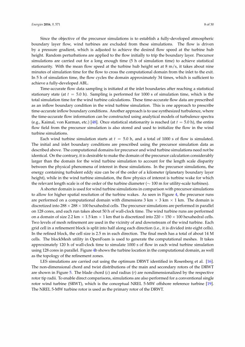
Since the objective of the precursor simulations is to establish a fully-developed atmosphericboundary layer flow, wind turbines are excluded from these simulations. The flow is drivenby a pressure gradient, which is adjusted to achieve the desired flow speed at the turbine hubheight. Random perturbations are applied to the flow initially to trip the boundary layer. Precursorsimulations are carried out for a long enough time (5 h of simulation time) to achieve statisticalstationarity. With the mean flow speed at the turbine hub height set at 8 m/s, it takes about nineminutes of simulation time for the flow to cross the computational domain from the inlet to the exit.In 5 h of simulation time, the flow cycles the domain approximately 34 times, which is sufficient toachieve a fully-developed ABL.

Time-accurate flow data sampling is initiated at the inlet boundaries after reaching a statisticalstationary state (at t = 5.0 h). Sampling is performed for 1000 s of simulation time, which is thetotal simulation time for the wind turbine calculations. These time-accurate flow data are prescribedas an inflow boundary condition in the wind turbine simulation. This is one approach to prescribetime-accurate inflow boundary conditions. Another approach is to use synthesized turbulence, wherethe time-accurate flow information can be constructed using analytical models of turbulence spectra(e.g., Kaimal, von Karman, etc.) [48]. Once statistical stationarity is reached (at t = 5.0 h), the entireflow field from the precursor simulation is also stored and used to initialize the flow in the windturbine simulations.

Each wind turbine simulation starts at t = 5.0 h, and a total of 1000 s of flow is simulated.The initial and inlet boundary conditions are prescribed using the precursor simulation data asdescribed above. The computational domains for precursor and wind turbine simulations need not beidentical. On the contrary, it is desirable to make the domain of the precursor calculation considerablylarger than the domain for the wind turbine simulation to account for the length scale disparitybetween the physical phenomena of interest in these simulations. In the precursor simulations, theenergy containing turbulent eddy size can be of the order of a kilometer (planetary boundary layerheight), while in the wind turbine simulation, the flow physics of interest is turbine wake for whichthe relevant length scale is of the order of the turbine diameter (∼ 100 m for utility-scale turbines).

A shorter domain is used for wind turbine simulations in comparison with precursor simulationsto allow for higher spatial resolution of the turbine wakes. As seen in Figure 4, the precursor runsare performed on a computational domain with dimensions 3 km × 3 km × 1 km. The domain isdiscretized into 288× 288× 100 hexahedral cells. The precursor simulations are performed in parallelon 128 cores, and each run takes about 50 h of wall-clock time. The wind turbine runs are performedon a domain of size 2.2 km × 1.5 km × 1 km that is discretized into 220× 150× 100 hexahedral cells.Two levels of mesh refinement are used in the vicinity of and downstream of the wind turbine. Eachgrid cell in a refinement block is split into half along each direction (i.e., it is divided into eight cells).In the refined block, the cell size is 2.5 m in each direction. The final mesh has a total of about 14 Mcells. The blockMesh utility in OpenFoam is used to generate the computational meshes. It takesapproximately 120 h of wall-clock time to simulate 1000 s of flow in each wind turbine simulationusing 128 cores in parallel. Figure 4b shows the turbine location in the computational domain, as wellas the topology of the refinement zones.

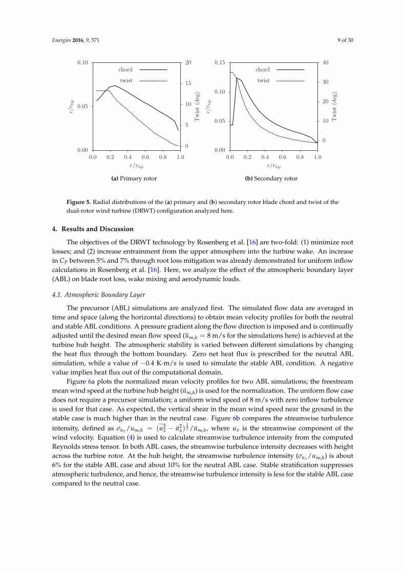
LES simulations are carried out using the optimum DRWT identified in Rosenberg et al. [16].The non-dimensional chord and twist distributions of the main and secondary rotors of the DRWTare shown in Figure 5. The blade chord (c) and radius (r) are nondimensionalized by the respectiverotor tip radii. To enable direct comparisons, simulations are also performed for a conventional singlerotor wind turbine (SRWT), which is the conceptual NREL 5-MW offshore reference turbine [19].The NREL 5-MW turbine rotor is used as the primary rotor of the DRWT.

Energies 2016, 9, 571 9 of 30

0.00

0.05

0.10

0.0 0.2 0.4 0.6 0.8 1.0

0

5

10

15

20c/r t

ip

Twist(deg)

r/rtip

chord

twist

(a) Primary rotor

0.00

0.05

0.10

0.15

0.0 0.2 0.4 0.6 0.8 1.0

0

10

20

30

40

c/r t

ip

Twist(deg)

r/rtip

chord

twist

(b) Secondary rotor

Figure 5. Radial distributions of the (a) primary and (b) secondary rotor blade chord and twist of thedual-rotor wind turbine (DRWT) configuration analyzed here.

4. Results and Discussion

The objectives of the DRWT technology by Rosenberg et al. [16] are two-fold: (1) minimize rootlosses; and (2) increase entrainment from the upper atmosphere into the turbine wake. An increasein CP between 5% and 7% through root loss mitigation was already demonstrated for uniform inflowcalculations in Rosenberg et al. [16]. Here, we analyze the effect of the atmospheric boundary layer(ABL) on blade root loss, wake mixing and aerodynamic loads.

4.1. Atmospheric Boundary Layer

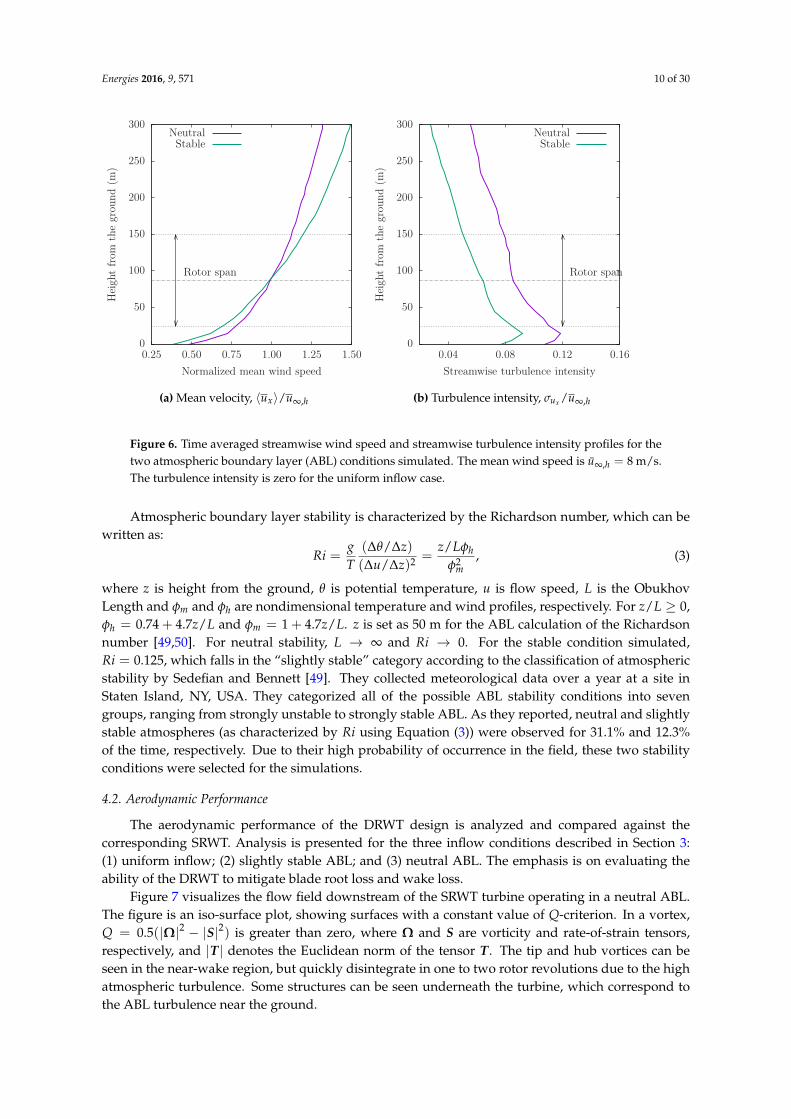
The precursor (ABL) simulations are analyzed first. The simulated flow data are averaged intime and space (along the horizontal directions) to obtain mean velocity profiles for both the neutraland stable ABL conditions. A pressure gradient along the flow direction is imposed and is continuallyadjusted until the desired mean flow speed (u∞,h = 8 m/s for the simulations here) is achieved at theturbine hub height. The atmospheric stability is varied between different simulations by changingthe heat flux through the bottom boundary. Zero net heat flux is prescribed for the neutral ABLsimulation, while a value of −0.4 K·m/s is used to simulate the stable ABL condition. A negativevalue implies heat flux out of the computational domain.

Figure 6a plots the normalized mean velocity profiles for two ABL simulations; the freestreammean wind speed at the turbine hub height (u∞,h) is used for the normalization. The uniform flow casedoes not require a precursor simulation; a uniform wind speed of 8 m/s with zero inflow turbulenceis used for that case. As expected, the vertical shear in the mean wind speed near the ground in thestable case is much higher than in the neutral case. Figure 6b compares the streamwise turbulenceintensity, defined as σux /u∞,h = (u2

x − u2x)

12 /u∞,h, where ux is the streamwise component of the

wind velocity. Equation (4) is used to calculate streamwise turbulence intensity from the computedReynolds stress tensor. In both ABL cases, the streamwise turbulence intensity decreases with heightacross the turbine rotor. At the hub height, the streamwise turbulence intensity (σux /u∞,h) is about6% for the stable ABL case and about 10% for the neutral ABL case. Stable stratification suppressesatmospheric turbulence, and hence, the streamwise turbulence intensity is less for the stable ABL casecompared to the neutral case.

Energies 2016, 9, 571 10 of 30

0

50

100

150

200

250

300

0.25 0.50 0.75 1.00 1.25 1.50

Rotor span

Heigh

tfrom

thegrou

nd(m

)

Normalized mean wind speed

NeutralStable

(a) Mean velocity, 〈ux〉/u∞,h

0

50

100

150

200

250

300

0.04 0.08 0.12 0.16

Rotor span

Heigh

tfrom

thegrou

nd(m

)Streamwise turbulence intensity

NeutralStable

(b) Turbulence intensity, σux /u∞,h

Figure 6. Time averaged streamwise wind speed and streamwise turbulence intensity profiles for thetwo atmospheric boundary layer (ABL) conditions simulated. The mean wind speed is u∞,h = 8 m/s.The turbulence intensity is zero for the uniform inflow case.

Atmospheric boundary layer stability is characterized by the Richardson number, which can bewritten as:

Ri =gT

(∆θ/∆z)(∆u/∆z)2 =

z/Lφhφ2

m, (3)

where z is height from the ground, θ is potential temperature, u is flow speed, L is the ObukhovLength and φm and φh are nondimensional temperature and wind profiles, respectively. For z/L ≥ 0,φh = 0.74 + 4.7z/L and φm = 1 + 4.7z/L. z is set as 50 m for the ABL calculation of the Richardsonnumber [49,50]. For neutral stability, L → ∞ and Ri → 0. For the stable condition simulated,Ri = 0.125, which falls in the “slightly stable” category according to the classification of atmosphericstability by Sedefian and Bennett [49]. They collected meteorological data over a year at a site inStaten Island, NY, USA. They categorized all of the possible ABL stability conditions into sevengroups, ranging from strongly unstable to strongly stable ABL. As they reported, neutral and slightlystable atmospheres (as characterized by Ri using Equation (3)) were observed for 31.1% and 12.3%of the time, respectively. Due to their high probability of occurrence in the field, these two stabilityconditions were selected for the simulations.

4.2. Aerodynamic Performance

The aerodynamic performance of the DRWT design is analyzed and compared against thecorresponding SRWT. Analysis is presented for the three inflow conditions described in Section 3:(1) uniform inflow; (2) slightly stable ABL; and (3) neutral ABL. The emphasis is on evaluating theability of the DRWT to mitigate blade root loss and wake loss.

Figure 7 visualizes the flow field downstream of the SRWT turbine operating in a neutral ABL.The figure is an iso-surface plot, showing surfaces with a constant value of Q-criterion. In a vortex,Q = 0.5(|Ω|2 − |S|2) is greater than zero, where Ω and S are vorticity and rate-of-strain tensors,respectively, and |T | denotes the Euclidean norm of the tensor T . The tip and hub vortices can beseen in the near-wake region, but quickly disintegrate in one to two rotor revolutions due to the highatmospheric turbulence. Some structures can be seen underneath the turbine, which correspond tothe ABL turbulence near the ground.

Energies 2016, 9, 571 11 of 30

Figure 7. Iso-surfaces of the Q-criterion of the SRWT operating in a neutral ABL. The contours arecolored by streamwise turbulence intensity: red and blue showing high and low turbulence intensitylevels, respectively.

4.2.1. Root Loss Mitigation

Airfoils in the root region (approximately inner 25%) of conventional turbine blades havevery high thickness-to-chord ratios and, thus, have poor aerodynamic performance. The smallersecondary rotor in the DRWT proposed by Rosenberg et al. [16] aims to mitigate the losses due to theaerodynamically non-optimum root region of the larger primary rotor blades. Since the secondaryrotor is much smaller in size compared to the primary rotor, it has significantly lower loads; loadsincrease in proportion with the cube of rotor diameter. The secondary rotor can therefore be designedusing relatively thin, aerodynamically-optimized airfoils that are efficient at extracting wind energypassing through the main rotor blade root region.

The CP of the DRWT is computed as the sum of the powers generated by the two rotors,normalized by the power in the wind going through the main rotor disk area. RANS calculations byRosenberg et al. [16] showed an increase in CP of about 7% with the DRWT. The results from the LESsimulations for the three inflow conditions, conducted as a part of this study, corroborate the findingsof Rosenberg et al. [16]. The DRWT outperforms the conventional SRWT for all inflow conditionsin terms of time-averaged power produced, demonstrating the “root loss mitigation” ability of theDRWT. There is also a marginal reduction in the time-averaged out-of-plane blade root bendingmoment (MOOP) of the primary rotor of the DRWT. A summary of these results is presented in Table 1.The percentage differences in the table are calculated as 100×(DRWT-SRWT)/SRWT. The largestincrease in power is observed for the neutral ABL condition and smallest for the uniform inflow case.

Table 1. Percentage difference in time-averaged turbine CP and MOOP.

Case %∆Power %∆MOOP

Uniform inflow 5.0 −0.39Stable ABL 5.4 −0.29

Neutral ABL 6.1 −0.07

Energies 2016, 9, 571 12 of 30

4.2.2. Turbine Wake Mixing

Comparative wake mixing analyses are performed for the DRWT and SRWT to investigate theability of the DRWT to reduce wake loss. The setup and inflow boundary condition for the neutraland stable cases are described in Section 3. For the uniform inflow simulation, the precursor runis not required, and a uniform wind velocity and zero turbulence intensity are specified at the inletboundaries. The flow angle is kept the same (30 degrees w.r.t. ex) as for the two ABL cases.

Mean Flow

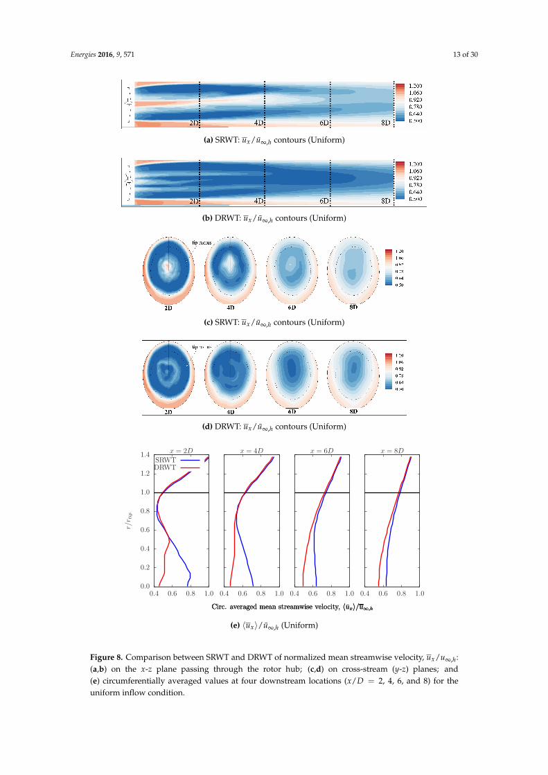
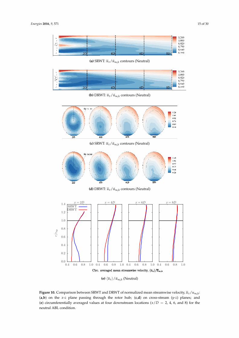
Time-averaged velocities in turbine wakes are compared first. Averaging is performed over110 revolutions of the main rotor. Large scale eddies in atmospheric turbulence contain significantenergy at frequencies much lower than rotor passing frequency; hence, averaging over a long time(in comparison with the rotor rotation period) is required. Contours of mean streamwise velocity areplotted on an x-z plane in the streamwise direction (see Subplots “a” and “b” in Figures 8–10) and ony− z planes in the cross-stream direction at four downstream locations: 2D, 4D, 6D and 8D, where Dis the main rotor diameter (see Subplots “c” and “d” in Figures 8–10). The cross-stream contour plotsare drawn over disks of a diameter 1.4-times the turbine rotor diameter, such that the top of each diskcorresponds to the 12 o’clock position of the rotor and the bottom to the six o’clock position; the viewis looking from downstream (but at an angle, so the disks look oval and not circular), and the mainturbine rotor is rotating counter-clockwise in the figures. The path traced by the rotor tip is markedwith the dashed curves. For a more quantitative comparison, streamwise velocity is azimuthally(circumferentially) averaged; averaging denoted by angle brackets as 〈ux〉. Radial profiles of 〈ux〉,normalized by u∞,h, are compared between the SRWT and the DRWT in the wake region (see, e.g.,Figure 8e).

Figure 8 compares the SRWT and DRWT designs for the uniform inflow case. Large differencesin mean velocities near the center of the disks are evident up to 8D downstream of the rotor.The SRWT is not effective at extracting energy from the wind in the blade root region, and hence,the wind flows through there unharvested. In contrast, the secondary rotor of the DRWT efficientlyextracts the energy from this streamtube and, hence, leaves a larger momentum (velocity) deficit in thewake. Reduced values of 〈ux〉/u∞,h are therefore observed in the wake of the DRWT as compared toSRWT for r/rtip < 0.4. This deficit reduces with downstream distance due to enhanced wake mixingin the DRWT. The circumferentially averaged plots show that by 8D downstream, the difference in thevelocity (and hence, kinetic energy) deficit between the DRWT and SRWT is considerably reduced.Also noted in the uniform inflow case is the slight flow acceleration near the ground under theturbines, which occurs due to the contraction of the streamtube caused by the slip wall boundarycondition imposed on the ground. As a result, the wake deficit shifts up and away from the groundas it convects downstream (see Figure 8).

The addition of the atmospheric boundary layer (ABL) considerably changes the turbineperformance and wake dynamics. The wall shear reduces the velocity near the ground. Hence, theacceleration effect observed in the uniform inflow case, due to streamtube contraction, is not observedin the ABL cases. The effect of wake rotation is evident in the ABL cases as seen by the azimuthallocations of highest mean velocity in Subplots (c) and (d) of Figures 9 and 10. The main rotors ofthe turbines are rotating in the counter-clockwise direction as seen from downstream, and the turbinewake rotates in the opposite (clockwise) direction. As the wake rotates, it pulls the higher momentumfluid from above (12 o’clock position), down and to the right in the figure (clockwise). Wake rotationalso pulls the low momentum fluid in the boundary layer near the ground, up and to the left inthe figures.

Energies 2016, 9, 571 13 of 30

(a) SRWT: ux/u∞,h contours (Uniform)

(b) DRWT: ux/u∞,h contours (Uniform)

(c) SRWT: ux/u∞,h contours (Uniform)

(d) DRWT: ux/u∞,h contours (Uniform)

0.0

0.2

0.4

0.6

0.8

1.0

1.2

1.4

0.4 0.6 0.8 1.0

Circ. averaged mean streamwise velocity, 〈ux〉/u∞,h

0.4 0.6 0.8 1.0

Circ. averaged mean streamwise velocity, 〈ux〉/u∞,h

0.4 0.6 0.8 1.0

Circ. averaged mean streamwise velocity, 〈ux〉/u∞,h

0.4 0.6 0.8 1.0

Circ. averaged mean streamwise velocity, 〈ux〉/u∞,h

r/r t

ip

x = 2D

SRWTDRWT

x = 4D x = 6D x = 8D

(e) 〈ux〉/u∞,h (Uniform)

Figure 8. Comparison between SRWT and DRWT of normalized mean streamwise velocity, ux/u∞,h:(a,b) on the x-z plane passing through the rotor hub; (c,d) on cross-stream (y-z) planes; and(e) circumferentially averaged values at four downstream locations (x/D = 2, 4, 6, and 8) for theuniform inflow condition.

Energies 2016, 9, 571 14 of 30

(a) SRWT: ux/u∞,h contours (Stable)

(b) DRWT: ux/u∞,h contours (Stable)

(c) SRWT: ux/u∞,h contours (Stable)

(d) DRWT: ux/u∞,h contours (Stable)

0.0

0.2

0.4

0.6

0.8

1.0

1.2

1.4

0.4 0.6 0.8 1.0

Circ. averaged mean streamwise velocity, 〈ux〉/u∞,h

0.4 0.6 0.8 1.0

Circ. averaged mean streamwise velocity, 〈ux〉/u∞,h

0.4 0.6 0.8 1.0

Circ. averaged mean streamwise velocity, 〈ux〉/u∞,h

0.4 0.6 0.8 1.0

Circ. averaged mean streamwise velocity, 〈ux〉/u∞,h

r/r t

ip

x = 2D

SRWTDRWT

x = 4D x = 6D x = 8D

(e) 〈ux〉/u∞,h (Stable)

Figure 9. Comparison between SRWT and DRWT of the normalized mean streamwise velocity,ux/u∞,h: (a,b) on the x-z plane passing through the rotor hub; (c,d) on cross-stream (y-z) planes;and (e) circumferentially averaged values at four downstream locations (x/D = 2, 4, 6, and 8) for thestable ABL condition.

Energies 2016, 9, 571 15 of 30

(a) SRWT: ux/u∞,h contours (Neutral)

(b) DRWT: ux/u∞,h contours (Neutral)

(c) SRWT: ux/u∞,h contours (Neutral)

(d) DRWT: ux/u∞,h contours (Neutral)

0.0

0.2

0.4

0.6

0.8

1.0

1.2

1.4

0.4 0.6 0.8 1.0

Circ. averaged mean streamwise velocity, 〈ux〉/u∞,h

0.4 0.6 0.8 1.0

Circ. averaged mean streamwise velocity, 〈ux〉/u∞,h

0.4 0.6 0.8 1.0

Circ. averaged mean streamwise velocity, 〈ux〉/u∞,h

0.4 0.6 0.8 1.0

Circ. averaged mean streamwise velocity, 〈ux〉/u∞,h

r/r t

ip

x = 2D

SRWTDRWT

x = 4D x = 6D x = 8D

(e) 〈ux〉/u∞,h (Neutral)

Figure 10. Comparison between SRWT and DRWT of normalized mean streamwise velocity, ux/u∞,h:(a,b) on the x-z plane passing through the rotor hub; (c,d) on cross-stream (y-z) planes; and(e) circumferentially averaged values at four downstream locations (x/D = 2, 4, 6, and 8) for theneutral ABL condition.

Energies 2016, 9, 571 16 of 30

The primary mechanism of wake mixing is turbulent momentum transport across the turbinewake layer, which is proportional to the turbulence level in the incoming wind. Higher turbulenceintensity in incoming flow therefore leads to a higher wake mixing rate. The turbulence in the ABLenhances wake mixing, and hence, the velocity deficits in the wakes are reduced for the two ABLcases in comparison with the uniform inflow case. The wake deficit for either turbine is highestfor the uniform flow case and smallest for the neutral ABL case. This behavior of the turbinewake mixing rate increasing with inflow turbulence intensity has been previously observed bothexperimentally [51] and numerically [52] for conventional, single-rotor turbines.

The interesting observation in the present study is that the difference in the velocity deficitsbetween the SRWT and DRWT also reduces faster for the ABL cases when compared to the uniformflow case; the difference is negligible by 8D downstream (compare Subplot “e” in Figures 9 and 10with Figure 8). This suggests that the presence of atmospheric turbulence enhances the wake mixingrate of the DRWT more than that of the SRWT. The increase in wake mixing rate is due to the ABLturbulence augmenting the interaction between the trailing wake/vortex systems of the two rotors ofthe DRWT; this interaction leads to increased turbulent momentum transport into the turbine wakelayer, as shown later in Section 4.2.3. The largest increase in wake mixing rate is observed for theneutral ABL case (Figure 10).

It should be noted that the secondary rotor of the DRWT used here is not specifically designedor operated to target wake mixing. The results obtained here, of enhanced wake mixing rate with aDRWT, indicate that the technology has potential to reduce wake losses if its design and operation areoptimized for that purpose. Furthermore, it is observed that even with the de facto design/operationof the DRWT, the additional wake deficit due to the secondary rotor of the DRWT is sufficiently mixedout such that it will not adversely impact the performance of the immediately downstream turbineif it is placed at least 8D away. Therefore, the gains achieved by mitigating root losses for isolatedturbines will be realized in array configurations (wind farms), as well.

Turbulence Intensity

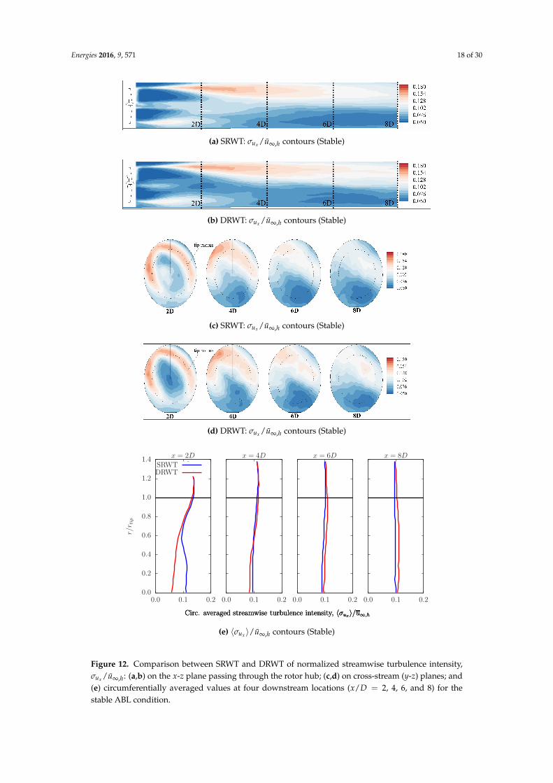
Mechanical turbulence, generated due to mean velocity shear in turbine wake and tip vortices,is an important contributor to wake mixing. Streamwise turbulence intensities in the wakes aretherefore compared between the DRWT and SRWT configurations for the three inflow conditionsin Figures 11–13. In all three cases, streamwise turbulence intensity near the turbine hub height ishigher for the SRWT until about 4D downstream of the turbine. This is because of two reasons:(1) due to the “leakage” of high-momentum fluid through the blade root region, a higher velocityshear is present in the wake of the SRWT than that of the DRWT; compare, e.g., Subplots (a) and (b)in Figure 8. Mean velocity shear is a source of turbulence; hence, there is higher shear-generatedturbulence in the wake of the SRWT near the turbine hub height up to 4D downstream of theturbine; and (2) the secondary rotor of the DRWT dampens the large scale eddies in the incomingABL flow. This phenomenon of a turbine rotor acting as a damper/high-pass filter has been reportedby Chamorro [53] for conventional single rotor wind turbines.

While the SRWT shows higher turbulence intensity in the wake up to about 4D, the turbulenceintensity for the DRWT is higher further downstream for all inflow conditions. This increase inturbulence production in the DRWT for x > 4D is due to the interaction between the trailingwake/vortex systems of the primary and the secondary rotors of the DRWT. The turbulenceproduction mechanism is velocity shear, which is increased by this interaction. Higher turbulenceintensity in the wake explains the higher wake mixing rate for the DRWT noted in the previoussection. The difference in turbulence intensities between the DRWT and the SRWT is highest for theneutral ABL case (which has the highest ABL turbulence of all of the cases simulated), re-emphasizingthat atmospheric turbulence promotes the interaction of the wake/vortex systems of the two rotors.

While increased turbulence intensity enhances the wake mixing rate and therefore boostswind farm efficiency, it does have a potential to increase fatigue loading on downstream turbines.

Energies 2016, 9, 571 17 of 30

This potential issue with the DRWT technology will be addressed in the future. Aerodynamic loadsfor a DRWT operating in “clean” flow, however, are analyzed in Section 4.3.

(a) SRWT: σux /u∞,h contours (Uniform)

(b) DRWT: σux /u∞,h contours (Uniform)

(c) SRWT: σux /u∞,h contours (Uniform)

(d) DRWT: σux /u∞,h contours (Uniform)

0.0

0.2

0.4

0.6

0.8

1.0

1.2

1.4

0.0 0.1 0.2

Circ. averaged streamwise turbulence intensity, 〈σux〉/u

∞,h

0.0 0.1 0.2

Circ. averaged streamwise turbulence intensity, 〈σux〉/u

∞,h

0.0 0.1 0.2

Circ. averaged streamwise turbulence intensity, 〈σux〉/u

∞,h

0.0 0.1 0.2

Circ. averaged streamwise turbulence intensity, 〈σux〉/u

∞,h

r/r t

ip

x = 2D

SRWTDRWT

x = 4D x = 6D x = 8D

(e) 〈σux 〉/u∞,h contours (Uniform)

Figure 11. Comparison between SRWT and DRWT of normalized streamwise turbulence intensity,σux /u∞,h: (a,b) on the x-z plane passing through the rotor hub; (c,d) on cross-stream (y-z) planes; and(e) circumferentially averaged values at four downstream locations (x/D = 2, 4, 6, and 8) for theuniform inflow condition.

Energies 2016, 9, 571 18 of 30

(a) SRWT: σux /u∞,h contours (Stable)

(b) DRWT: σux /u∞,h contours (Stable)

(c) SRWT: σux /u∞,h contours (Stable)

(d) DRWT: σux /u∞,h contours (Stable)

0.0

0.2

0.4

0.6

0.8

1.0

1.2

1.4

0.0 0.1 0.2

Circ. averaged streamwise turbulence intensity, 〈σux〉/u

∞,h

0.0 0.1 0.2

Circ. averaged streamwise turbulence intensity, 〈σux〉/u

∞,h

0.0 0.1 0.2

Circ. averaged streamwise turbulence intensity, 〈σux〉/u

∞,h

0.0 0.1 0.2

Circ. averaged streamwise turbulence intensity, 〈σux〉/u

∞,h

r/r t

ip

x = 2D

SRWTDRWT

x = 4D x = 6D x = 8D

(e) 〈σux 〉/u∞,h contours (Stable)

Figure 12. Comparison between SRWT and DRWT of normalized streamwise turbulence intensity,σux /u∞,h: (a,b) on the x-z plane passing through the rotor hub; (c,d) on cross-stream (y-z) planes; and(e) circumferentially averaged values at four downstream locations (x/D = 2, 4, 6, and 8) for thestable ABL condition.

Energies 2016, 9, 571 19 of 30

(a) SRWT: σux /u∞,h contours (Neutral)

(b) DRWT: σux /u∞,h contours (Neutral)

(c) SRWT: σux /u∞,h contours (Neutral)

(d) DRWT: σux /u∞,h contours (Neutral)

0.0

0.2

0.4

0.6

0.8

1.0

1.2

1.4

0.0 0.1 0.2

Circ. averaged streamwise turbulence intensity, 〈σux〉/u

∞,h

0.0 0.1 0.2

Circ. averaged streamwise turbulence intensity, 〈σux〉/u

∞,h

0.0 0.1 0.2

Circ. averaged streamwise turbulence intensity, 〈σux〉/u

∞,h

0.0 0.1 0.2

Circ. averaged streamwise turbulence intensity, 〈σux〉/u

∞,h

r/r t

ip

x = 2D

SRWTDRWT

x = 4D x = 6D x = 8D

(e) 〈σux 〉/u∞,h contours (Neutral)

Figure 13. Comparison between SRWT and DRWT of normalized streamwise turbulence intensity,σux /u∞,h: (a,b) on the x-z plane passing through the rotor hub; (c,d) on cross-stream (y-z) planes; and(e) circumferentially averaged values at four downstream locations (x/D = 2, 4, 6, and 8) for theneutral ABL condition.

Energies 2016, 9, 571 20 of 30

4.2.3. Momentum Entrainment

Utility-scale turbines in wind farms are typically installed in systematic arrangements (arrays).Wake losses in a wind farm are most severe when the wind direction is aligned with the turbine rows.In such extreme cases, it is meaningful to look into the entrainment of high-momentum fluid into theturbine wake layer. For a very large, closely-packed turbine array, the turbine wake layer would behorizontal, stretching vertically from H − rtip to H + rtip, where H is the turbine hub height and rtipis the rotor tip radius. For an isolated turbine analysis, however, the turbine wake layer is cylindrical,co-axial with the rotor, and has the same diameter as that of the turbine rotor (see Figure 14).

Turbulent transport of momentum from outside the turbine layer has been identified tobe the dominant mechanism for re-energizing the flow in large wind turbine arrays [54].Turbulent momentum flux through the cylindrical turbine wake layer (see Figure 14) is analyzed tocompute turbulent momentum and energy transport and investigate wake recharging. The presentanalysis is performed for a turbine wake layer that extends from the turbine rotor location to 8Ddownstream. Time averaged velocity and the Reynolds stress tensor (u′iu

′j) are interpolated onto this

cylindrical surface using the Tecplot 360 software (www.tecplot.com).

Turbine wake layer

(a) Schematic (b) Turbine wake layer (cylindrical surface)

Figure 14. Investigation of turbulent momentum transport into the turbine wake layer:(a) a schematic; and (b) cylindrical surface showing the turbine wake layer through which turbulentmomentum flux is computed to quantify entrainment in the turbine wake.

Entrainment of high momentum fluid into this cylinder is induced by turbulent stresses,particularly the stress term u′ru′x, where the subscript “r” denotes the radial component, the primedenotes a perturbation quantity and the overline denotes a time-averaged quantity. A cylindricalcoordinate system (er, eθ , ex) with its axis aligned with the freestream flow direction ex is used (seeAppendix A). Equation (6) relates u′ru′x to the Reynolds stress tensor computed in the ground frameof reference (ex, ey, ez). Since er points radially outward, a negative value of u′ru′x implies transportinto the cylinder (turbine wake layer).

Figure 15a–f plots the Reynolds stress term u′ru′x normalized by u2∞,h on the unwrapped

cylindrical surface that defines the turbine layer. The color map in the figure is reversed to makeintuitive sense: negative values indicate net flux into the cylinder. In the figure, θ = 0 correspondsto the 12 o’clock position and ±180 correspond to the six o’clock position. It can be noticed thatthe highest value of −u′ru′x is not at the 12 o’clock position, but skewed about it. This behaviorhas been noted previously by Wu and Porté Agel [55], although for the stress term u′xu′z. A cleartrend of increasing momentum entrainment with increasing ABL turbulence is seen in the figure forboth SRWT and DRWT. The x-location where peak entrainment occurs varies both with atmosphericturbulence intensity and azimuthal location. The peak values occur closer to the turbine as inflowturbulence intensity increases (compare Subplot “a” with “b” and “c” of Figure 15). This is because

Energies 2016, 9, 571 21 of 30

the incoming turbulence disintegrates the tip vortex system quickly. For ABL cases, peak −u′ru′xoccurs around one rotor diameter downstream of the turbine near the ground (θ =±180), while nearthe 12 o’clock position, the peak values occur further downstream.

(a) SRWT Uniform (b) SRWT Stable (c) SRWT Neutral

(d) DRWT Uniform (e) DRWT Stable (f) DRWT Neutral

-1.2E-02

-8.0E-03

-4.0E-03

0.0E+000 2 4 6 8

Turb

mom

flux,〈u

′ ru′ x〉/u2 ∞

,h

x/D

SRWTDRWT

(g) Uniform

-1.2E-02

-8.0E-03

-4.0E-03

0.0E+000 2 4 6 8

Turb

mom

flux,〈u

′ ru′ x〉/u2 ∞

,h

x/D

SRWTDRWT

(h) Stable

-1.2E-02

-8.0E-03

-4.0E-03

0.0E+000 2 4 6 8

Turb

mom

flux,〈u

′ ru′ x〉/u2 ∞

,h

x/D

SRWTDRWT

(i) Neutral

Figure 15. Radial transport of streamwise momentum into the turbine wake layer. Color contoursshow u′ru′x/u2

∞,h on the cylindrical surface of Figure 14 that has been cut at θ =±180 and unwrapped.

While there is a significant difference in the spatial distribution and magnitudes of u′ru′x betweenthe three inflow conditions considered, the differences between the SRWT and DRWT are subtle.The DRWT shows a higher level of momentum entrainment, especially for x > 5D. To calculatenet entrainment from all around the cylinder, u′ru′x is further averaged azimuthally. The azimuthalaveraging operation is denoted by angle brackets; thus, the quantity 〈u′ru′x〉 represents the temporally-and spatially-averaged value of u′ru′x. 〈u′ru′x〉 multiplied by the circumference of the cylinder (2πrtip)is the turbulent momentum entrainment per unit length into the cylinder. Subplots (g–i) in Figure 15show the variation of 〈u′ru′x〉 (normalized by u2

∞,h) with distance from the turbine rotor location.

Energies 2016, 9, 571 22 of 30

The y−axis is reversed in the plots as negative values imply positive entrainment. Variation isplotted on the same scale to contrast the mixing rates between the different inflow conditions. Theneutral ABL case shows the highest entrainment, while the uniform inflow case shows the lowestentrainment. The plots for the turbulent flux of kinetic energy (ux × u′ru′x) are very similar to thosefor momentum flux and, hence, are not shown.

The overall percentage changes in turbulent flux of axial momentum and kinetic energy dueto the DRWT are provided in Table 2. The increase in entrainment for the DRWT over the SRWTis highest for the neutral ABL case and lowest (indeed there is a slight reduction) for the uniforminflow case. A modest 3.29% increase in momentum entrainment is observed for the neutral case.The reader is reminded that in these simulations, the secondary rotor is operated at the tip speedratio that gives the maximum aerodynamic performance for isolated turbine operation in uniforminflow conditions. No attempt is made here to optimize the secondary rotor design/operation toenhance wake mixing. Notwithstanding the sub-optimal design/operation, the DRWT still showshigher levels of entrainment than the SRWT for the two ABL cases. These results demonstrate that ina wind farm, the turbines operating in wake flow can benefit from enhanced entrainment providedby the DRWT. Additionally, the fact that the turbine operation and the geometry of the secondaryrotor can be optimized to actively target wake mixing leaves potential for further improvement inwind farm efficiency from the DRWT technology.

Table 2. Percent change (DRWT-SRWT) in cumulative streamwise momentum and kinetic energy forthe three inflow conditions.

Inflow Condition %∆(u′ru′x) %∆(ux× u′ru′x)

Uniform −1.17% −2.30%Stable +1.78% +1.63%

Neutral +3.29% +2.54%

4.3. Aerodynamic Loads

Aerodynamic loads in terms of blade root bending moments are analyzed in this section.The approximations made to carry out this analysis are: (1) the rotor blades are assumed to beinfinitely rigid (i.e., no deformation in turbine geometry is permitted); (2) the turbine is operated ata fixed rotation rate irrespective of the incoming wind speed (hence, the tip speed ratio is fluctuatingdue to inflow turbulence); and (3) the blade geometry is not resolved in the simulations, and hence,the potential interaction between the rotors due to blade thickness is not captured.

Figures 16 and 17 compare the turbine power and out-of-plane blade root bending moment(MOOP) in the time and frequency domains for the two ABL cases simulated. The dynamic loadsin the uniform flow case are very small compared to the ABL cases, and hence, those results are notpresented. For the DRWT, turbine power is the sum of powers from the two rotors; blade root momenthowever is only compared for the main rotor unless otherwise stated. Figure 16 compares the DRWTand SRWT power and loads for the stable ABL condition. The secondary rotor in the DRWT efficientlyextracts power near the main rotor blade root region, and hence, the DRWT produces higher netpower than the SRWT (see Subplot “a” in Figures 16 and 17). In the plots, power is normalized by1/2ρu3

∞,h Ad and blade root bending moments by 1/2ρu2∞,h Ad rt, where Ad = πr2

t and rt is the mainrotor tip radius.

Fluctuations in power output are caused by spatial and temporal variations of the incomingwind. While the temporal variations are only due to turbulence, spatial variations also occur in themean wind speed in the ABL; the mean wind speed varies monotonically with height from the groundin the area swept by the turbine rotor (see Figure 6a). Each blade of the turbine rotor(s) experiencesa one per revolution variation/excitation because of this spatial variation of the mean wind speed— highest wind at the 12 o’clock position and lowest at the six o’clock position. This periodic (since

Energies 2016, 9, 571 23 of 30

the rotor rotation speed is fixed) excitation results in deterministic fluctuations in turbine power andblade loads. The torque contribution from each blade of a turbine rotor adds linearly (scalar addition)to give the net rotor torque (and power); blade root bending moments however are about differentaxes for each blade, so they need to be added as vectors in order to compute the moment on theturbine shaft. Here, we analyze blade root moments. Since the turbine blades are assumed to beidentical, one-per-revolution fluctuation in the torque/power for each blade causes a one-per-BPFvariation in torque/power for the rotor, where BPF stands for blade passing frequency. Blade rootbending moments however are for each rotor blade, which therefore fluctuate at the fundamentalfrequency of one per turbine revolution, or 1/rev.

0.30

0.40

0.50

0.60

0.70

0 20 40 60 80 100 120

Pow

er/(

1 2ρu3 ∞

,hA

d)

Number of rotor revolutions

SRWTDRWT

(a) Time variation of normalized turbine power

0.10

0.15

0.20

0.25

0.30

0 20 40 60 80 100 120

Mom

ent/(

1 2ρu2 ∞

,hA

dr t)

Number of rotor revolutions

SRWTDRWT

(b) Time variation of normalized MOOP

106

107

108

109

1010

0.1 1 10

PSD

ofrotorpow

er(W

2/H

z)

Frequency / rotor passing freq.

SRWTDRWT

(c) PSD of turbine power

107

108

109

1010

1011

1012

0.1 1 10

PSD

ofroot

MOOP,(N

.m)2/H

z

Frequency / rotor passing freq.

SRWTDRWT

(d) PSD of MOOP

Figure 16. Stable ABL simulation results. Turbine power and out-of-plane blade root bending moment(MOOP) compared in the time and frequency domains.

Energies 2016, 9, 571 24 of 30

0.30

0.40

0.50

0.60

0.70

0 20 40 60 80 100 120

Pow

er/(

1 2ρu3 ∞

,hA

d)

Number of rotor revolutions

SRWTDRWT

(a) Time variation of normalized turbine power

0.10

0.15

0.20

0.25

0.30

0 20 40 60 80 100 120

Mom

ent/(

1 2ρu2 ∞

,hA

dr t)

Number of rotor revolutions

SRWTDRWT

(b) Time variation of normalized MOOP

106

107

108

109

1010

0.1 1 10

PSD

ofrotorpow

er(W

2/H

z)

Frequency / rotor passing freq.

SRWTDRWT

(c) PSD of turbine power

107

108

109

1010

1011

1012

0.1 1 10

PSD

ofroot

MOOP,(N

.m)2/H

z

Frequency / rotor passing freq.

SRWTDRWT

(d) PSD of MOOP

Figure 17. Neutral ABL simulation results. Turbine power and out-of-plane blade root bendingmoment (MOOP) compared in the time and frequency domains.

Deterministic power fluctuations at the BPF and its harmonics are observed in the power spectraldensity (PSD) plots (see Subplot “c” in Figures 16 and 17) due to the variation of mean wind speedwith height as discussed above. In these figures, the main rotor passing frequency is used tonormalize frequency. Power fluctuations at secondary rotor passing frequency and its harmonics arealso present, but they are much smaller in magnitude and are therefore inconspicuous in the figure.While the increase in mean power from the DRWT is measurable (between 5% and 6%), the change(reduction) in power fluctuations observed is insignificant. Power fluctuations are not desirable, andhence, no increase in such fluctuations with the DRWT is beneficial. The difference in out-of-planeblade root bending moment (MOOP) is also insignificant; the DRWT showing a very small reduction at

Energies 2016, 9, 571 25 of 30

high harmonics of rotor passing frequency (see Figure 17). The reduction is expected to be small sincethe contribution to the root bending moment from the blade root region, where the blade relative flowvelocity and the moment arm are both small, is insignificant. The results suggest that the aerodynamicinteraction between the main rotor and the secondary rotor has little impact on unsteady aerodynamicloads experienced by the main rotor.

Figure 18 compares the MOOP for the SRWT operating in the stable and neutral ABL conditions.The PSD of the MOOP is higher for the stable case at the fundamental rotor passing frequency becausethe vertical shear in the mean wind speed is higher for the stable case (see Figure 6a). Vertical shearin mean wind results in a 1/rev variation in the angle-of-attack, and hence, loads, on the rotorblades. At frequencies greater than the fundamental rotor passing frequency, the neutral case showshigher values of MOOP than the stable case. This behavior can be explained by the difference inthe size of the turbulent eddies in the two ABL cases. A wind turbine rotor can “chop” througha large, slow-moving turbulent eddy multiple times, resulting in blade loads at the rotor passingfrequency and its harmonics. The integral length scale represents the size of the largest eddies ina turbulent flow. In the present problem, the integral length scale is computed at the hub heightusing a two-point correlation of streamwise wind velocity, defined as Ruu(r) = 〈u(x) u(x + r ex)〉,where the angle brackets denote spatial averaging over the horizontal plane at the turbine hub height(x.ez = h) and the overline denotes time averaging. The two-point correlations are computed usingthe precursor simulations for the two ABL cases and are compared in Figure 18b. The integral lengthscale (L) is computed as L =

∫ Rmax0 Ruu(r)dr, where the upper limit of the integral Rmax = 3 km.

The integral lengths are found to be approximately 24 m and 130 m for the stable and neutral ABLcases, respectively. The higher values of MOOP at frequencies greater than the fundamental rotorpassing frequency can be attributed to the larger eddy sizes (higher integral length scale) in theneutral ABL case.

107

108

109

1010

1011

1012

0.1 1 10

PSD

ofroot

MOOP((N.m

)2/H

z)

Frequency / rotor passing freq.

NeutralStable

(a) MOOP for the SRWT in ABL

-0.25

0.00

0.25

0.50

0.75

1.00

1.25

0 200 400 600 800 1000

Autocorrelation,R

uu(r)

Separation, r (m)

NeutralStable

(b) Velocity autocorrelation

Figure 18. Autocorrelation of the velocity fluctuation as a function of distance.

Secondary Rotor

Figure 19 presents the power spectral densities of the secondary rotor MOOP for neutral andstable conditions. Contrasting the magnitudes in Figure 19 with those in Figures 16 and 17 elucidatesthat the mean and the fluctuating loads on the secondary rotor are in fact orders of magnitude smallerthan those on the main rotor. Therefore, the secondary rotor can be designed with relatively thinairfoils. The abscissa in Figure 19 is normalized by the secondary rotor blade passing frequency.

Energies 2016, 9, 571 26 of 30

While the decay in power spectral density with frequency is monotonic for the main rotor, which isnot the case with the secondary rotor. The MOOP at the fourth harmonic of the rotor passing frequencyis higher than the second and third harmonics. This is likely an effect of the aerodynamic interactionbetween the main and the secondary rotors.

102

103

104

105

106

107

108

0.1 1 10

PSD

ofroot

MOOP,(N

.m)2/H

z

Frequency / rotor passing freq.

NeutralStable

Figure 19. Secondary rotor simulation results.

5. Conclusions

A numerical study is conducted using large eddy simulations to investigate aerodynamicperformance and loads for the dual rotor wind turbine (DRWT) technology proposed byRosenberg et al. [16]. The LES solver is first validated against experimental data, as well as bladeelement momentum theory results for a conventional, single-rotor turbine. A two-step procedureis used to first simulate the atmospheric boundary layer and then wind turbine aerodynamics.The DRWT is analyzed for three different inflow conditions: uniform inflow, stable and neutralatmospheric boundary layer. The following conclusions are drawn from the results of this study.

1. The DRWT operating in isolation shows aerodynamic performance (CP) improvement of about5%–6% for all inflow conditions. The performance benefit is obtained due to efficient extractionof energy (using the smaller secondary rotor) from the streamtube going through the bladeroot region.

2. The DRWT enhances wake mixing and entrainment of higher momentum fluid from outsidethe wake layer when the atmospheric (freestream) turbulence is moderately high (as in theneutral stability case simulated here). A modest (≈ 3.2%) increase in momentum entrainment isobserved with the de facto DRWT design.

3. The enhancement in wake mixing is associated with the increased turbulence intensity in thewake. This could potentially increase fatigue loads on the downstream turbines.

4. Spectral analysis of aerodynamic loads (measured as rotor power and out-of-plane blade rootmoment) shows negligible reduction for the main rotor in the DRWT. Unsteady fluctuations inrotor power are observed at blade passing frequency, while fluctuations in blade root momentsare at the rotor passing frequency and its harmonics. These fluctuations occur because of theazimuthal variation (due to the ABL) in the incoming mean wind, as well as turbulence inthe wind.

Energies 2016, 9, 571 27 of 30

The enhanced wake mixing rate observed with the DRWT is promising. It proves that thetechnology has the potential to improve wind farm efficiency if the secondary rotor is optimallydesigned and/or operated for that purpose.

Acknowledgments: Funding for this work was provided by the National Science Foundation under GrantNumber NSF/CBET-1438099 and the Iowa Energy Center under Grant Number 14-008-OG. The numericalsimulations reported here were performed using the NSF Extreme Science and Engineering DiscoveryEnvironment (XSEDE) resources available to the authors under Grant Number TG-CTS130004 and partlythrough the High Performance Computing (HPC) equipment at the Iowa State University, some of whichhas been purchased through funding provided by NSF under Major Research Instrumentation Grant NumberCNS 1229081.

Author Contributions: Behnam Moghadassian performed the atmospheric boundary layer and wind turbinesimulations and processed those results. Aaron Rosenberg performed the LES validation against experimentaldata and BEM theory. Anupam Sharma conceived of the simulations and the DRWT design. All authorscontributed to the writing of the manuscript.

Conflicts of Interest: The authors declare no conflict of interest.

Appendix Coordinate Systems

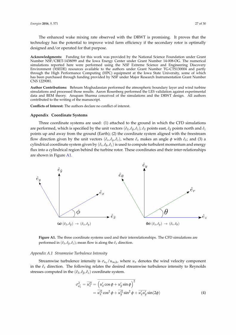
Three coordinate systems are used: (1) attached to the ground in which the CFD simulationsare performed, which is specified by the unit vectors (ex, ey, ez); ex points east, ey points north and ez

points up and away from the ground (Earth); (2) the coordinate system aligned with the freestreamflow direction given by the unit vectors (ex, ey, ez), where ex makes an angle φ with ex; and (3) acylindrical coordinate system given by (er, eθ , ez) is used to compute turbulent momentum and energyflux into a cylindrical region behind the turbine rotor. These coordinates and their inter-relationshipsare shown in Figure A1.

(a) (ex, ey) → (ex, ey) (b) (ex, ey) → (er, eθ)

Figure A1. The three coordinate systems used and their interrelationships. The CFD simulations areperformed in (ex, ey, ez); mean flow is along the ex direction.

Appendix A.1 Streamwise Turbulence Intensity

Streamwise turbulence intensity is σux /u∞,h, where ux denotes the wind velocity componentin the ex direction. The following relates the desired streamwise turbulence intensity to Reynoldsstresses computed in the (ex, ey, ez) coordinate system.

σ2u′x

= u′2x =(

u′x cos φ + u′y sin φ)2

= u′2x cos2 φ + u′2y sin2 φ + u′xu′y sin(2φ) (4)

Energies 2016, 9, 571 28 of 30

Appendix A.2 Streamwise Turbulent Momentum and Energy Flux

Streamwise turbulent momentum flux through the circular cylinder in Figure 14 is determinedby integrating the Reynolds stress term u′ru′x over the cylinder surface. u′ru′x is related to the Reynoldsstress defined in the (ex, ey, ez) coordinate system as follows:

u′ru′x = (u′z cos θ + u′y sin θ)× (u′x cos φ + u′y sin φ)

=(

u′xu′z cos φ + u′yu′z sin φ)

cos θ +(

u′xu′y cos φ + u′yu′y sin φ)

sin θ, (5)

where,

u′xu′y = u′xu′y cos φ− u′2x sin φ, and

u′yu′y = u′2y cos φ− u′xu′y sin φ.

Using these in Equation (5) gives:

u′ru′x =(

u′xu′z cos φ + u′yu′z sin φ)

cos θ

+

(u′xu′y cos2 φ− u′xu′y sin2 φ + u′2y

sin(2φ)

2− u′2x

sin(2φ)

2

)sin θ,

or, u′ru′x =(

u′xu′z cos φ + u′yu′z sin φ)

cos θ

+

(u′xu′y cos(2φ) + (u′2y − u′2x )

sin(2φ)

2

)sin θ. (6)

The turbulent energy flux is obtained by integrating the following over the surface.

ux × u′ru′x = u′x cos φ + u′y sin φ× u′ru′x (7)

References

1. Sharma, A.; Taghaddosi, F.; Gupta, A. Diagnosis of Aerodynamic Losses in the Root Region of a HorizontalAxis Wind Turbine; General Electric Company Technical Report; General Electric Global Research Center:Niskayuna, NY, USA, 2010.

2. Barthelmie, R.J.; Jensen, L.E. Evaluation of power losses due to wind turbine wakes at the Nysted offshorewind farm. Wind Energy 2010, 13, 573–586.

3. Baker, J.; Mayda, E.; Van Dam, C. Experimental analysis of thick blunt trailing-edge wind turbine airfoils.J. Solar Energy Eng. 2006, 128, 422–431.

4. Fuglsang, P.; Bak, C. Development of the Risø Wind Turbine Airfoils. Wind Energy 2004, 7, 145–162.5. Kusiak, A.; Song, Z. Design of wind farm layout for maximum wind energy capture. Renew. Energy 2010,

35, 685–694.6. González, J.S.; Rodriguez, A.G.G.; Mora, J.C.; Santos, J.R.; Payan, M.B. Optimization of wind farm turbines

layout using an evolutive algorithm. Renew. Energy 2010, 35, 1671–1681.7. Mittal, P.; Kulkarni, K.; Mitra, K. A novel hybrid optimization methodology to optimize the total number

and placement of wind turbines. Renew. Energy 2016, 86, 133–147.8. Dabiri, J.O. Potential order-of-magnitude enhancement of wind farm power density via counter-rotating

vertical-axis wind turbine arrays. J. Renew. Sustain. Energy 2011, 3, 043104.9. Corten, G.P.; Lindenburg, K.; Schaak, P. Assembly of Energy Flow Collectors, Such as Windpark, and

Method of Operation, U.S. Patent 7,299,627, 27 November 2007.10. Jiménez, Á.; Crespo, A.; Migoya, E. Application of a LES technique to characterize the wake deflection of a

wind turbine in yaw. Wind energy 2010, 13, 559–572.11. Westergaard, C.H. Method for Improving Large Array Wind Park Power Performance Through Active

Wake Manipulation Reducing Shadow Effects, U.S. Patent App. 14/344,284, 21 March 2012.

Energies 2016, 9, 571 29 of 30

12. Newman, B. Multiple Actuator-Disc Theory for Wind Turbines. J. Wind Eng. Ind. Aerodyn. 1986, 24,215–225.

13. Jung, S.N.; No, T.S.; Ryu, K.W. Aerodynamic performance prediction of a 30kW counter-rotating windturbine system. Renew. Energy 2005, 30, 631–644.

14. Kanemoto, T.; Galal, A.M. Development of intelligent wind turbine generator with tandem wind rotorsand double rotational armatures (1st report, superior operation of tandem wind rotors). JSME Int. J. Ser. B2006, 49, 450–457.

15. Kanemoto, T. Wind Turbine Generator. U.S. Patent App. 13/147,021, 19 April 2010.16. Rosenberg, A.; Selvaraj, S.; Sharma, A. A Novel Dual-Rotor Turbine for Increased Wind Energy Capture.

J. Phys. Conf. Ser. 2014, 524, 012078.17. Rosenberg, A.; Sharma, A. A Prescribed-Wake Vortex Lattice Method for Aerodynamic Analysis and

Optimization of Co-Axial, Dual-Rotor Wind Turbines. ASME J. Solar Energy Eng. 2016, submitted.18. Selvaraj, S. Numerical Investigation of Wind Turbine and Wind Farm Aerodynamics. Master’s Thesis,

Iowa State University, Ames, IA, USA, 2014.19. Jonkman, J.; Butterfield, S.; Musial, W.; Scott, G. Definition of a 5-MW Reference Wind Turbine for Offshore

System Development; NREL: Golden, CO, USA, 2009.20. Mikkelsen, R. Actuator Disk Models Applied to Wind Turbines. Ph.D. Thesis, Technical University of

Denmark, Copenhagen, Denmark, 2003.21. Betz, A. Schraubenpropeller mit Geringstem Energieverlust. Nachrichten von der Gesellschaft der

Wissenschafte n zu Göttingen, Mathematisch-Physikalische Klasse, 1919, 193-217.22. Goldstein, S. On the vortex theory of screw propellers. R. Soc. 1929, 123, 440–465.23. Burton, T.; Sharpe, D.; Jenkins, N.; Bossanyi, E. Wind Energy Handbook; John Wiley & Sons Ltd.: Chichester,

UK, 2002.24. Ainslie, J.F. Calculating the Flow Field in the Wake of Wind Turbines. J. Wind Eng. Ind. Aerodyn. 1988,

27, 213–224.25. Snel, H. Review of Aerodynamics for Wind Turbines. Wind Energy 2003, 6, 203–211.26. Calaf, M.; Meneveau, C.; Meyers, J. Large eddy simulation study of fully developed wind-turbine array

boundary layers. Phys. Fluids 2010, 22, 015110.27. Vermeer, L.J.; Sørensen, J.N.; Crespo, A. Wind Turbine Wake Aerodynamics. Prog. Aerosp. Sci. 2003, 39,

467–510.28. Sanderse, B.; van der Pijl, S.P.; Koren, B. Review of Computational Fluids Dynamics for Wind Turbine Wake

Aerodynamics. Wind Energy 2011, doi:10.1002/we.458.29. Jimenez, A.; Crespo, A.; Migoya, E.; Garcia, J. Advances in Large-Eddy Simulation of a Wind Turbine Wake.

J. Phys. Conf. Ser. 2007, 75, 015004.30. Jimenez, A.; Crespo, A.; Migoya, E.; Garica, J. Large Eddy Simulation of Spectral Coherence in a Wind

Turbine Wake. Environ. Res. Lett. 2008, 3, 015004.31. Porté-Agel, F.; Wu, Y.; Lu, H.; Conzemius, R.J. Large-Eddy Simulation of Atmospheric Boundary Layer

Flow through Wind Turbines and Wind Farms. J. Wind Eng. Ind. Aerodyn. 2011, 99, 154–168.32. Wu, Y.; Porté-Agel, F. Large-Eddy Simulation of Wind-Turbine Wakes: Evaluation of Turbine

Parametrisations. Bound. Layer Meteorol. 2011, 138, 345–366.33. Troldborg, N.; Larsen, G.C.; Madsen, H.A.; Hansen, K.S.; Sørensen, J.N.; Mikkelsen, R. Numerical

simulations of wake interaction between two wind turbines at various inflow conditions. Wind Energy2011, 14, 859–876.

34. Porté-Agel, F.; Wu, Y.T.; Chen, C.H. A numerical study of the effects of wind direction on turbine wakesand power losses in a large wind farm. Energies 2013, 6, 5297–5313.

35. Stevens, R.J.; Gayme, D.F.; Meneveau, C. Large eddy simulation studies of the effects of alignment andwind farm length. J. Renew. Sustain. Energy 2014, 6, 023105.

36. Churchfield, M.J.; Lee, S.; Michalakes, J.; Moriarty, P.J. A numerical study of the effects of atmospheric andwake turbulence on wind turbine dynamics. J. Turbul. 2012, 13, 1–32.

37. Churchfield, M.; Lee, S.; Moriarty, P. A Large-Eddy Simulation of Wind-Plant Aerodynamics.In Proceedings of the 50th AIAA Aerospace Sciences Meeting including the New Horizons Forum andAerospace Exposition, Nashville, TN, USA, 9–12 January 2012.

Energies 2016, 9, 571 30 of 30

38. Smagorinsky, J. General Circulation Experiments with the Primitive Equations I. The Basic Experiment.Monthly Weather Rev. 1963, 91, 99–164.

39. Lilly, D.K. A proposed modification of the Germano subgrid-scale closure method. Phys. Fluids A Fluid Dyn.(1989–1993) 1992, 4, 633–635.

40. Germano, M.; Piomelli, U.; Moin, P.; Cabot, W.H. A dynamic subgrid-scale eddy viscosity model.Phys. Fluids A Fluid Dyn. (1989–1993) 1991, 3, 1760–1765.

41. Churchfield, M.; Lee, S. NWTC Design Codes (SOWFA). Available online: http://wind.nrel.gov/designcodes/simulators/SOWFA (accessed on 6 July 2016).

42. Moeng, C. A Large-Eddy-Simulation Model for the Study of Planetary Boundary-Layer Turbulence.J. Atmosp. Sci. 1984, 41, 2052–2062.

43. Stull, R.B. An Introduction to Boundary Layer Meteorology; Kluwer Academic Publishers: Dordecht,The Netherlands, 1988.

44. Lee, S.; Churchfield, M.; Moriarty, P.; Jonkman, J.; Michalakes, J. Atmospheric and wake turbulence impactson wind turbine fatigue loadings. AIAA Paper 2012-0540, 2012. Available online: http://www.nrel.gov/docs/fy12osti/53567.pdf (accessed on 21 July 2016)

45. Jonkman, J.; Buhl, M. FAST User’s Guide; NREL Technical Report No. NREL/EL-500-38230, NationalRenewable Energy Laboratory: Golden, CO, USA, 2005.

46. Schepers, J.; Brand, A.; Bruining, A.; Graham, J.; Hand, M.; Infield, D.; Madsen, H.; Paynter, R.; Simms, D.Final Report of IEA Annex XIV: Field Rotor Aerodynamics; Technical Report ECN-C-97-027; Energy ResearchCenter of the Netherlands: Petten, The Netherlands, 1997.

47. Organization, W.M. Guide to Meteorological Instruments and Methods of Observation; Secretariat of the WorldMeteorological Organization: Geneva, Switzerland, 1983.

48. Davidson, L. HYBRID LES-RANS: Inlet Boundary Conditions for Flows with Recirculation. In Advances inHybrid RANS-LES Modelling; Springer: Berlin, Germany, 2008; pp. 55–66.

49. Sedefian, L.; Bennett, E. A comparison of turbulence classification schemes. Atmosp. Environ. (1967) 1980,14, 741–750.

50. Businger, J.A. Turbulent transfer in the atmospheric surface layer. Q. J. R. Meteorol. Soc. 1972, 98, 67–100.51. Chamorro, L.P.; Porté-Agel, F. Effects of thermal stability and incoming boundary-layer flow characteristics

on wind-turbine wakes: A wind-tunnel study. Bound. Layer Meteorol. 2010, 136, 515–533.52. Jha, P.K.; Duque, E.P.; Bashioum, J.L.; Schmitz, S. Unraveling the Mysteries of Turbulence Transport in a

Wind Farm. Energies 2015, 8, 6468–6496.53. Chamorro, L.; Guala, M.; Arndt, R.; Sotiropoulos, F. On the evolution of turbulent scales in the wake of a

wind turbine model. J. Turbul. 2012, 13, doi:10.1080/14685248.2012.69716954. Cal, R.B.; Lebrón, J.; Castillo, L.; Kang, H.S.; Meneveau, C. Experimental study of the horizontally averaged

flow structure in a model wind-turbine array boundary layer. J. Renew. Sustain. Energy 2010, 2, 013106.55. Wu, Y.T.; Porté-Agel, F. Large-eddy simulation of wind-turbine wakes: Evaluation of turbine

parametrisations. Bound. Layer Meteorol. 2011, 138, 345–366.

c© 2016 by the authors; licensee MDPI, Basel, Switzerland. This article is an open accessarticle distributed under the terms and conditions of the Creative Commons Attribution(CC-BY) license (http://creativecommons.org/licenses/by/4.0/).