Embed Size (px)
Citation preview
Numerical Investigation of Wind Turbine and Wind Farm Aerodynamics
by
Suganthi Selvaraj
A thesis submitted to the graduate faculty
in partial fulfillment of the requirements for the degree of
MASTER OF SCIENCE
Major: Aerospace Engineering
Program of Study Committee:
Anupam Sharma, Major Professor
Eugene Takle
Hui Hu
Iowa State University
Ames, Iowa
2014
Copyright Suganthi Selvaraj, 2014. All rights reserved.

ii
DEDICATION
For their constant support, their unmovable devotion and loyalty to my dreams and ambi-
tions, I dedicate this thesis to my parents, Dr. Selvaraj Rajendran and Dr. Eunice Selvaraj,
and my brother, Dhanraj Selvaraj. I pray that this accomplishment brings you some measure
of joy because it would not be possible without your example of faith, love and dedication.
iii
TABLE OF CONTENTS
LIST OF FIGURES . . . . . . . . . . . . . . . . . . . . . . . . . . . . . . . . . . . v
ACKNOWLEDGEMENTS . . . . . . . . . . . . . . . . . . . . . . . . . . . . . . . ix
ABSTRACT . . . . . . . . . . . . . . . . . . . . . . . . . . . . . . . . . . . . . . . . x
CHAPTER 1. Wind Turbine Aerodynamics . . . . . . . . . . . . . . . . . . . . 1
1.1 Introduction . . . . . . . . . . . . . . . . . . . . . . . . . . . . . . . . . . . . . . 1
1.2 C
P
Entitlement for a HAWT Operating in Isolation in Uniform Flow . . . . . . 4
1.2.1 1-D Momentum Theory . . . . . . . . . . . . . . . . . . . . . . . . . . . 5
1.2.2 Actuator Disk With Swirl . . . . . . . . . . . . . . . . . . . . . . . . . . 7
1.2.3 E↵ect of Finite Number of Blades . . . . . . . . . . . . . . . . . . . . . 8
1.2.4 E↵ect of Viscosity . . . . . . . . . . . . . . . . . . . . . . . . . . . . . . 9
1.3 Numerical modeling of wind turbine aerodynamics . . . . . . . . . . . . . . . . 11
1.3.1 Airfoil force distribution . . . . . . . . . . . . . . . . . . . . . . . . . . . 12
1.3.2 Gaussian Distribution of forces . . . . . . . . . . . . . . . . . . . . . . . 13
1.3.3 Simulation set-up . . . . . . . . . . . . . . . . . . . . . . . . . . . . . . . 16
1.3.4 Validation . . . . . . . . . . . . . . . . . . . . . . . . . . . . . . . . . . . 16
1.4 Conclusion . . . . . . . . . . . . . . . . . . . . . . . . . . . . . . . . . . . . . . 22
CHAPTER 2. Investigation of a Novel, Dual Rotor Wind Turbine Concept . 28
2.1 Numerical Simulations using RANS CFD . . . . . . . . . . . . . . . . . . . . . 32
2.1.1 Simulation set-up . . . . . . . . . . . . . . . . . . . . . . . . . . . . . . . 33
2.1.2 Rotor Design . . . . . . . . . . . . . . . . . . . . . . . . . . . . . . . . . 34
2.1.3 Optimization Study . . . . . . . . . . . . . . . . . . . . . . . . . . . . . 34
2.1.4 Large Eddy Simulations . . . . . . . . . . . . . . . . . . . . . . . . . . . 37
iv
2.2 Conclusion . . . . . . . . . . . . . . . . . . . . . . . . . . . . . . . . . . . . . . 38
CHAPTER 3. Wind Farm Aerodynamics . . . . . . . . . . . . . . . . . . . . . . 42
3.1 Surface Flow Convergence in Wind Farms . . . . . . . . . . . . . . . . . . . . . 44
3.2 Numerical simulations . . . . . . . . . . . . . . . . . . . . . . . . . . . . . . . . 45
3.2.1 Problem set-up . . . . . . . . . . . . . . . . . . . . . . . . . . . . . . . . 45
3.2.2 Boundary conditions . . . . . . . . . . . . . . . . . . . . . . . . . . . . . 46
3.2.3 Atmospheric stability conditions . . . . . . . . . . . . . . . . . . . . . . 48
3.2.4 Concept Simulation . . . . . . . . . . . . . . . . . . . . . . . . . . . . . 49
3.2.5 Story County Wind Farm Simulation . . . . . . . . . . . . . . . . . . . . 53
3.3 Conclusion . . . . . . . . . . . . . . . . . . . . . . . . . . . . . . . . . . . . . . 56
v
LIST OF FIGURES
1.1 Current installed wind capacity in the USA [1] . . . . . . . . . . . . . . 2
1.2 Annual and cumulative wind installations by 2030 [1] . . . . . . . . . . 3
1.3 A schematic of the proposed dual rotor wind turbine (DRWT) concept 4
1.4 An illustration of the flow convergence phenomenon. The slanted arrow
on the left refers to the incoming freestream velocity direction and the
arrow on the right refers to the turned velocity due to flow convergence 5
1.5 Illustration of 4 cross sections in the actuator disk method . . . . . . . 5
1.6 Evolution of pressure and velocity through an actuator disk . . . . . . 6
1.7 C
P
and C
T
values as functions of induction, a from the 1-D momentum
theory. . . . . . . . . . . . . . . . . . . . . . . . . . . . . . . . . . . . . 7
1.8 Variation of (a) axial & swirl induction with �r
, and (b) maximum C
P
as a function of �. . . . . . . . . . . . . . . . . . . . . . . . . . . . . . . 8
1.9 C
P
versus � curves for varying number of blades of a HAWT. Taken
from Okulov [33]. . . . . . . . . . . . . . . . . . . . . . . . . . . . . . . 10
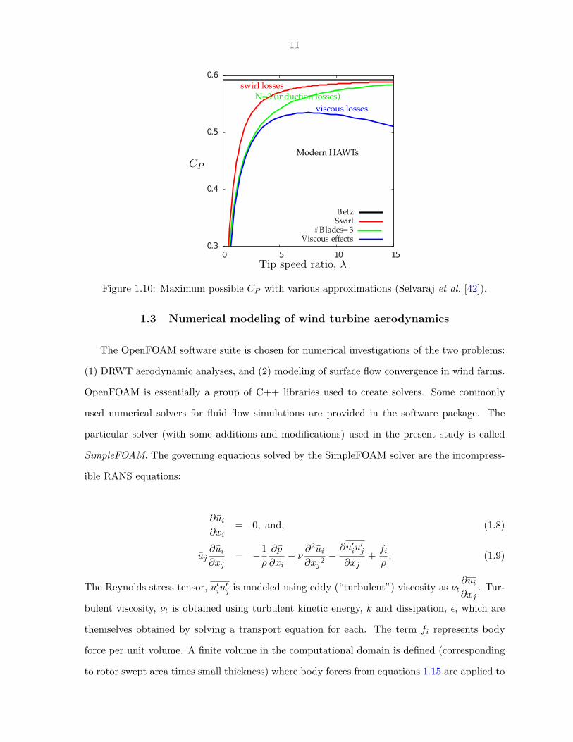
1.10 Maximum possible C
P
with various approximations (Selvaraj et al. [42]). 11
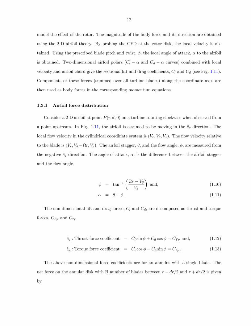
1.11 Airfoil . . . . . . . . . . . . . . . . . . . . . . . . . . . . . . . . . . . . 13
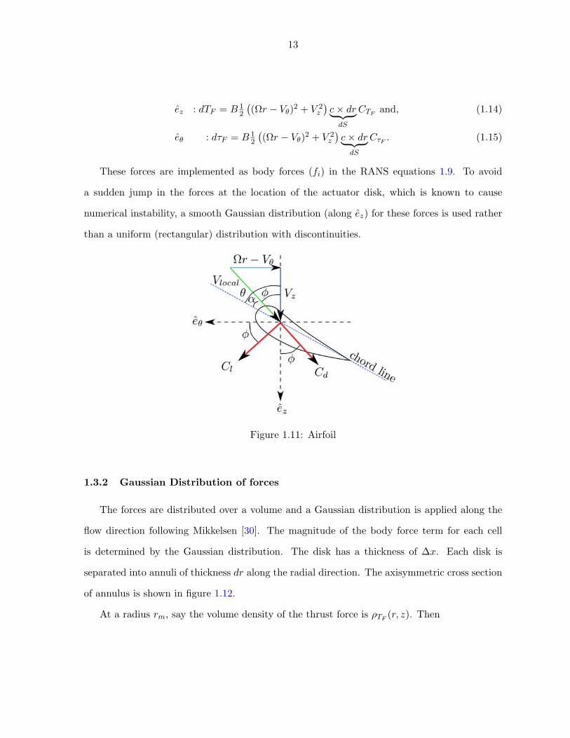
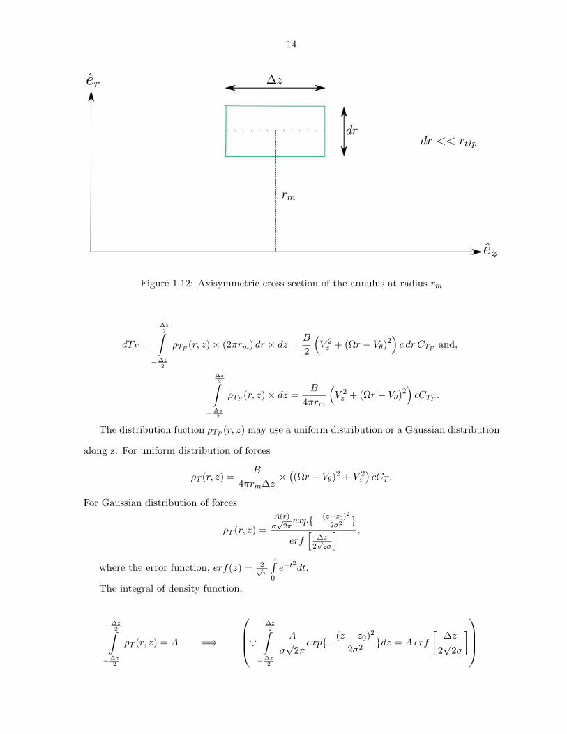
1.12 Axisymmetric cross section of the annulus at radius r
m
. . . . . . . . . 14
1.13 Illustration of Gaussian distribution . . . . . . . . . . . . . . . . . . . . 15
1.14 2-D simulation schematic . . . . . . . . . . . . . . . . . . . . . . . . . . 16
1.15 Illustration of a wedge mesh . . . . . . . . . . . . . . . . . . . . . . . . 17
1.16 Two dimensional grid for the uniformly loaded rotor . . . . . . . . . . 18
1.17 Simulation of the uniformly loaded rotor using a = 0.1 . . . . . . . . . 19
1.18 Simulation of the uniformly loaded rotor using a = 0.5 . . . . . . . . . 20
vi
1.19 Validation against analytical results using 1D momentum theory for C
T
and C
P
. Plot on the right uses the computed value of ‘a’ on the abscissa. 21
1.20 Geometric chord and twist distribution for the Ris� rotor . . . . . . . 22
1.21 Cp � � comparison between various measured data, BEM theory and
actuator disk simulation results. . . . . . . . . . . . . . . . . . . . . . . 23
1.22 Pressure contours and streamlines through the Risoe Turbine (actuator
disk simulation results) for tip speed ratio, � = 4.0. . . . . . . . . . . . 24
1.23 Pressure contours and streamlines through the Risoe Turbine (actuator
disk simulation results) for tip speed ratio, � = 7.0. . . . . . . . . . . . 24
1.24 Torque force coe�cient, c
⌧
and thrust force coe�cient, c
N
distributions
compared between Actuator disk model predictions against BEM pre-
diction. . . . . . . . . . . . . . . . . . . . . . . . . . . . . . . . . . . . . 25
1.25 Geometric chord and twist distribution for the NREL phase VI rotor . 25
1.26 Cp� � curve. . . . . . . . . . . . . . . . . . . . . . . . . . . . . . . . . 26
1.27 Pressure contours and streamlines through the NREL-VI Turbine (ac-
tuator disk simulation results) for tip speed ratio, � = 4.0 . . . . . . . 26
1.28 Pressure contours and streamlines through the NREL-VI Turbine (ac-
tuator disk simulation results) for tip speed ratio, � = 7.0 . . . . . . . 27
1.29 Torque force coe�cient, c
⌧
and thrust force coe�cient, c
N
distributions
compared between Actuator disk model predictions against BEM results. 27
2.1 Maximum possible C
P
with various approximations (Selvaraj et al. [42]). 29
2.2 Family of airfoils for a medium NREL blade (Tangler et al. [46]). . . . 29
2.3 A schematic of the proposed dual-rotor concept. . . . . . . . . . . . . . 30
2.4 Comparison of numerically predicted and analytically evaluated (by
Newman [32]) C
T
and C
P
for a 4-disk turbine. . . . . . . . . . . . . . . 33
2.5 Comparison of numerically predicted and analytically evaluated (by
Newman [32]) C
T
and C
P
for a 3-disk turbine. . . . . . . . . . . . . . . 33
vii
2.6 Comparison of numerically predicted and analytically evaluated (by
Newman [32]) C
T
and C
P
for a 2-disk turbine. . . . . . . . . . . . . . . 34
2.7 Radial distributions of (a) input (a and C
l
) and (b) output (blade chord
and twist) for the secondary rotor with the DU96 airfoil. . . . . . . . . 35
2.8 The lift and drag coe�cient polars for the DU96 airfoil . . . . . . . . . 36
2.9 The radial chord and twist distributions of the NREL 5MW turbine. . 37
2.10 Simulations for two di↵erent rotor sizes showing pressure contours and
streamlines . . . . . . . . . . . . . . . . . . . . . . . . . . . . . . . . . . 38
2.11 �C
P
(DRWT - SRWT), di↵erence in aerodynamic power coe�cient,
�C
P
= C
P
DRWT
� C
P
SRWT
due to the addition of a secondary rotor. . 39
2.12 Simulations for two axial separation distances showing pressure contours
and streamlines . . . . . . . . . . . . . . . . . . . . . . . . . . . . . . . 39
2.13 �C
P
(DRWT - SRWT), di↵erence in aerodynamic power coe�cient,
�C
P
= C
P
DRWT
� C
P
SRWT
due to the addition of a secondary rotor. . 40
2.14 Radial distribution of the torque force coe�cient for the main rotor,
secondary rotor and the main rotor operating in isolation. . . . . . . . 40
2.15 Radial distribution of the angle of attack for the main rotor, secondary
rotor and the main rotor operating in isolation. . . . . . . . . . . . . . 41
2.16 A snapshot of iso-surfaces of Q-criterion from the DRWT LES simulation. 41
3.1 The phenomenon of flow convergence in wind farms. (a) A schematic
illustrating micro-scale pressure gradient that is set up by turbines in a
wind farm, and (b) CWEX measurements of resulting flow convergence
in neutral atmospheric stability condition. . . . . . . . . . . . . . . . . 44
3.2 The di↵erent refinement regions for a turbine . . . . . . . . . . . . . . 46
3.3 Inlet velocity profile for inviscid and viscous simulations . . . . . . . . 47
3.4 The di↵erent atmospheric stability conditions [18]. . . . . . . . . . . . 48
3.5 Simulation setup and mesh at turbine hub height. . . . . . . . . . . . . 49
viii
3.6 Inviscid simulation: Kinematic pressure contours drawn (a) at hub
height and (b) on the ground. . . . . . . . . . . . . . . . . . . . . . . . 50
3.7 Inviscid simulation: flow angle (w.r.t. x direction) contours drawn (a)
at hub height and (b) on the ground. . . . . . . . . . . . . . . . . . . . 51
3.8 Average (over Y direction) pressure and flow angle on the ground versus
distance along the turbine array. . . . . . . . . . . . . . . . . . . . . . . 52
3.9 Kinematic pressure contours drawn (a) at hub height and (b) on the
ground. . . . . . . . . . . . . . . . . . . . . . . . . . . . . . . . . . . . . 53
3.10 Flow angle contours drawn (a) at hub height and (b) on the ground. . 54
3.11 Average (over Y direction) pressure and flow angle on the ground versus
distance along the turbine array. . . . . . . . . . . . . . . . . . . . . . . 55
3.12 Layout of the story county farm turbines. The locations denoted by the
circles in the red box are the locations of the meteorological towers. . . 57
3.13 Relative locations of the meteorological towers and the turbines in the
Story County wind farm. The hollow rectangles denote turbine locations
and the filled circles denote meteorological tower locations. . . . . . . . 58
3.14 Simulation results for case A. Contours of (a) pressure and (b) flow
angle, drawn on a plane at a height of 0.27⇥ r
tip
above the ground. . . 58
3.15 Simulation results for case A. Contours of (a) pressure and (b) flow
angle, drawn on a plane at a height of 0.27⇥ r
tip
above the ground. . . 59
3.16 Simulation results for case B. Contours of (a) pressure and (b) flow
angle, drawn on a plane at a height of 0.27⇥ r
tip
above the ground. . . 59
3.17 Simulation results for case B. Contours of (a) pressure and (b) flow
angle, drawn on a plane at a height of 0.27⇥ r
tip
above the ground. . . 60
3.18 Change in flow angle (w.r.t. the value at M1) as functions of distance
from B2 turbine for (a) case A, and (b) case B. . . . . . . . . . . . . . 60
ix
ACKNOWLEDGEMENTS
For good health, the strength, the perseverance, the blessing of opportunities, first and
most importantly, I thank my Father, God Almighty. Without His grace and love, I would not
be who I am and where I am today.
To Dr. Anupam Sharma, my major professor, I would like to express my deepest apprecia-
tion. Without his guidance, persistent encouragement and advice, this dissertation would still
be a figment of my imagination. Dr. Sharma has been more than just a source of knowledge
and under his mentorship, I have drawn much inspiration from his personable and patient
nature.
To the members of my Program of Study(PoS) committee, Dr. Eugene Takle and Dr. Hui
Hu, I express my gratitude for their e↵orts in helping me successfully complete this work.
To Dan Rajewski, I express my gratitude for his time in providing me with the necessary
experimental data.
To my colleagues who through blood, sweat and tears became friends, Karthik Reddy,
Varun Vikas, Lei Shi, Meilin Yu, Ben Zimmerman, Daniel Garrick, Bharat Agrawal, Aaron
Rosenberg and Behnam Moghadassian, I thank you for the invaluable, educational discourses.
Your support meant more to me than you will ever know.
I would also like to express my appreciation to Dr. Paul Durbin, Dr. Zhi J. Wang and Dr.
Ganesh Rajagopalan whose inspirational conversations, lectures and teaching styles stoked the
ember of a passion for CFD.
To the lovely aerospace engineering o�ce sta↵, Gayle Fay and Laurie Hoidfelt, for patiently
holding my hand through the mountains of paperwork.
Last but certainly not least, I thank my parents and brother who have been a continuous
source of encouragment and support. I would also like to thank all my family and friends for
the immense emotional and mental support throughout this endeavour.
x
ABSTRACT
A numerical method based on the solution of Reynolds Averaged Navier Stokes equations
and actuator disk respresentation of turbine rotor is developed and implemented in the Open-
FOAM software suite for aerodynamic analysis of horizontal axis wind turbines (HAWT). The
method and the implementation are validated against the 1-D momentum theory, the blade
element momentum theory and against experimental data. The model is used for analyzing
aerodynamics of a novel dual rotor wind turbine concept and wind farms.
Horizontal axis wind turbines su↵er from aerodynamic ine�ciencies in the blade root region
(near the hub) due to several non-aerodynamic constraints (e.g., manufacturing, transportation,
cost, etc.). A new dual-rotor wind turbine (DRWT) concept is proposed that aims at mitigating
these losses. A DRWT is designed that uses an existing turbine rotor for the main rotor (an
NREL 5 MW rotor design), while the secondary rotor is designed using a high lift to drag
ratio airfoil (the DU 96 airfoil from TU Delft). The numerical aerodynamic analyses method
developed as a part of this thesis is used to optimize the design. The new DRWT design gives
an improvement of about 7% in aerodynamic e�ciency over the single rotor turbine.
Wind turbines are typically deployed in clusters called wind farms. HAWTs also su↵er from
aerodynamic losses in a wind farm due to interactions with wind turbine wakes. An interesting
mesoscale meteorological phenomenon called “surface flow convergence” believed to be caused
by wind turbine arrays is investigated using the numerical method developed here. This phe-
nomenon is believed to be caused by the pressure gradient set up by wind turbines operating
in close proximity in a farm. A conceptual/hypothetical wind farm simulation validates the
hypothesis that a pressure gradient is setup in wind farms due to turbines and that it can
cause flow veering of the order of 10 degrees. Simulations of a real wind farm (Story County)
are also conducted which give qualitatively correct flow direction change, however quantitative
agreement with data is only moderately acceptable.
1
CHAPTER 1. Wind Turbine Aerodynamics
A basic description of the 1-D momentum theory along with e↵ects of swirl and finite
number of blades is presented in this chapter. The actuator disk theory to model wind tur-
bine aerodynamics is also provided with validation again experimental data and against other
theories.
1.1 Introduction
Electricity is an important part of our every day lives. In this day and age, electricity is used
for virtually every task, regardless of complexity. The need for energy sources is ever increasing
while natural resources such as coal, petroleum and natural gas are rapidly depleting. Thus
we look to sustainable energy resources such as solar, wind, etc. The most invested form of
sustainable(renewable) energy source in the last few years is wind [15].
The United States Department of Energy investigated the implications if 20% of the nation’s
electricity demand were to be provided by wind by the year 2030. As of November 2013, 4.16%
of the nation’s electricity demand was provided by wind[11]. By the year 2030, the electricity
demand in the US is predicted to increase by 39%. To meet 20% of that demand, the wind
capacity would have to reach more than 300 GW. Currently, 61.108 GW are available in the
US Fig. 1.1. If we assume all the wind turbines are of 2 MW capacity, then 30000 additional
such turbines need to be deployed to reach the target milestone. This is roughly equal to eight
times the number of turbines currently installed in the USA.
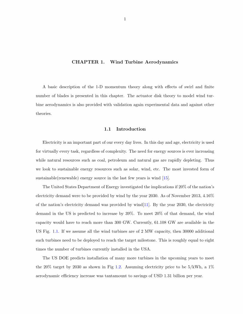
The US DOE predicts installation of many more turbines in the upcoming years to meet
the 20% target by 2030 as shown in Fig 1.2. Assuming electricity price to be 5/kWh, a 1%
aerodynamic e�ciency increase was tantamount to savings of USD 1.31 billion per year.

2
Hence, research on improving e�ciency of wind farms and individual turbines is worthwhile.
Several investigations ([3], [29], [51])are being done to understand and eventually improve the
e�ciency of a turbine and wind farms. Two such investigations are performed and described
in this thesis.
Figure 1.1: Current installed wind capacity in the USA [1]
The Betz-Lancaster-Zhukowski limit of aerodynamic power coe�cient, C
P
= 16/27 is often
casually referred to as the highest obtainable e�ciency of a single-rotor horizontal axis wind
turbine (HAWT). The realizable, practical limit of a torque-based, finite-bladed HAWT, op-
erating in a viscous fluid is actually much lower [49]. A more “practical” limit on C
P
for a
single-rotor HAWT is thus proposed. After accounting for these (almost unavoidable) physical
limits, this “practical” limit on C
P
is found to be just a few percentage points higher than that
of modern, utility-scale HAWTs.
A novel dual rotor wind turbine (DRWT) concept is proposed and analyzed for its aero-
3
Figure 1.2: Annual and cumulative wind installations by 2030 [1]
dynamic performance. The motivation for this comes from the fact that wind turbine blades
have high aerodynamic losses near the root of the blades (approximately bottom 25%). That
particular region of the blade is primarily designed for maintaining the structural integrity of
the blade. It causes high aerodynamic losses and thus reduces the overall e�ciency of a turbine.
A new, dual-rotor design is proposed to mitigate these losses by introducing another rotor of a
smaller size upstream of the main rotor (See Figure 1.3). Secondary rotor e�ciently captures
the power lost due to the aerodynamic ine�ciency of the main rotor in the root region.
Most utility scale turbines are deployed in clusters and due to aerodynamic interactions
between turbines in a cluster, they do not operate in isolation. Barthelmie et al. [5] shows that
up to 40% losses occur in a wind farm due to wake interaction between turbines. Therefore, it
is important to study aerodynamic interaction of turbines in a wind farm in order to improve
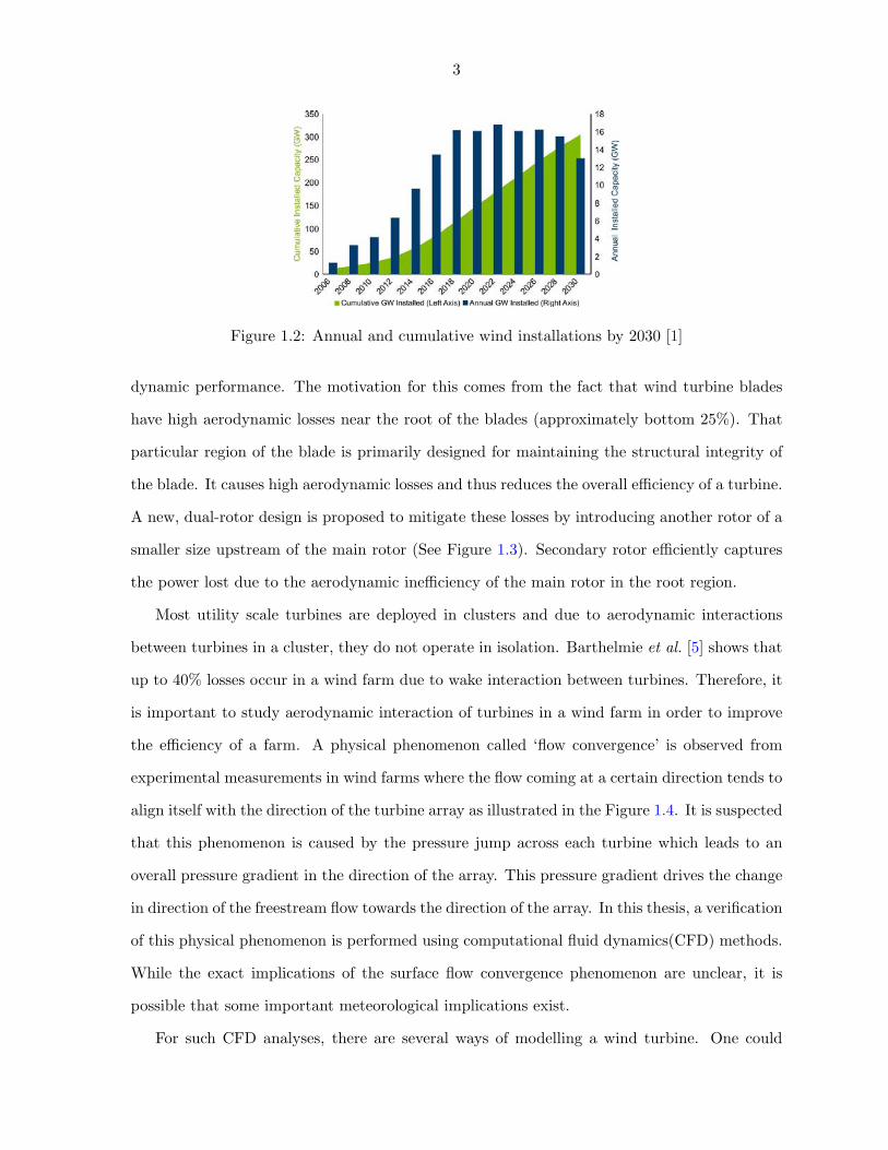
the e�ciency of a farm. A physical phenomenon called ‘flow convergence’ is observed from
experimental measurements in wind farms where the flow coming at a certain direction tends to
align itself with the direction of the turbine array as illustrated in the Figure 1.4. It is suspected
that this phenomenon is caused by the pressure jump across each turbine which leads to an
overall pressure gradient in the direction of the array. This pressure gradient drives the change
in direction of the freestream flow towards the direction of the array. In this thesis, a verification
of this physical phenomenon is performed using computational fluid dynamics(CFD) methods.
While the exact implications of the surface flow convergence phenomenon are unclear, it is
possible that some important meteorological implications exist.
For such CFD analyses, there are several ways of modelling a wind turbine. One could

4
Figure 1.3: A schematic of the proposed dual rotor wind turbine (DRWT) concept
build a model of the entire turbine using a CAD package or assume and take advantage of flow
symmetry and periodicity between blade passages to simulate only one blade passage (e.g., a
120� for a 3-bladed HAWT). Such methods are computationally expensive even for a single
turbine. Hence, a more feasible actuator disk method that does not resolve the blade geometry
in the simulation but models its e↵ect using body forces is adopted in this study. This approach
gives substantial computation time savings.
1.2 CP
Entitlement for a HAWT Operating in Isolation in Uniform Flow
Several theories with varying degrees of approximations are available to analyze aerody-
namic e�ciency of a horizontal axis wind turbine (HAWT). The simplifications in these the-
ories typically neglect one or more physical phenomena that reduce the practically attainable
e�ciency. The simplest of these theories, for example, is the 1-D momentum theory that gives
the Betz limit [7] for aerodynamic e�ciency of a HAWT of C
P
= 16/27(⇠ 0.593). The turbine
5
Figure 1.4: An illustration of the flow convergence phenomenon. The slanted arrow on the leftrefers to the incoming freestream velocity direction and the arrow on the right refers to theturned velocity due to flow convergence
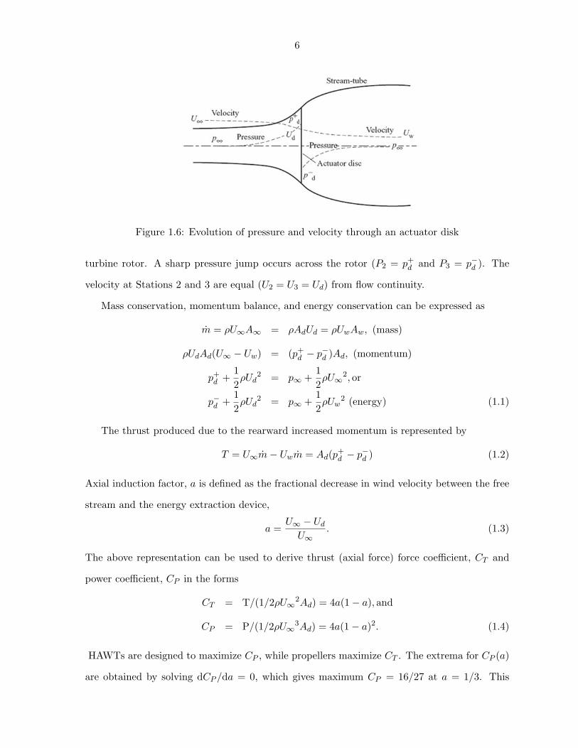
rotor is represented by an actuator disk that supports a pressure jump across it. Figure 1.6
shows a schematic of the actuator disk model.
1.2.1 1-D Momentum Theory
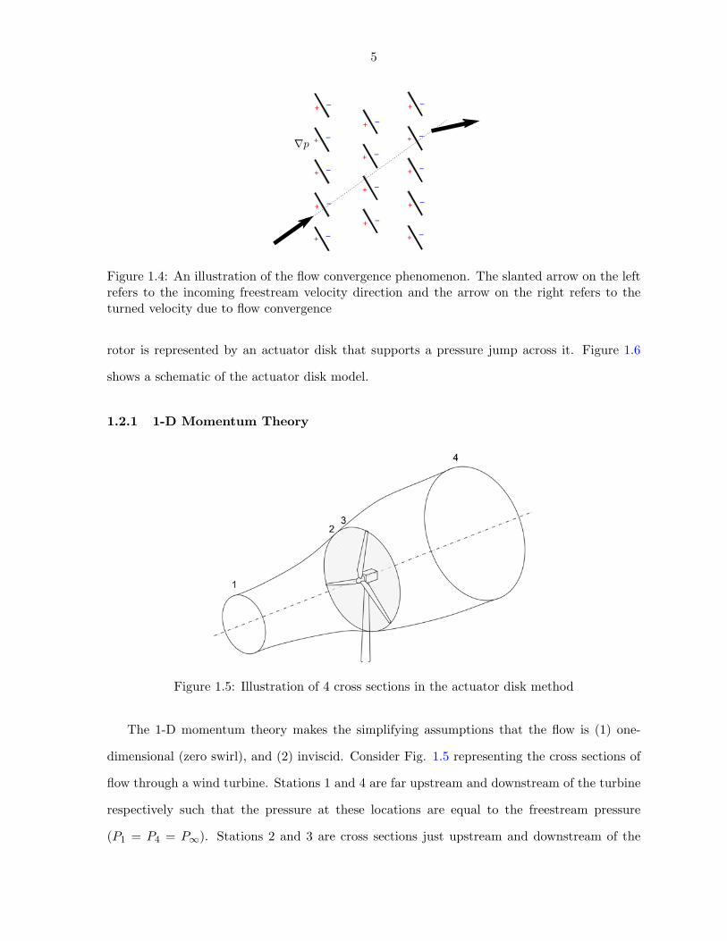
Figure 1.5: Illustration of 4 cross sections in the actuator disk method
The 1-D momentum theory makes the simplifying assumptions that the flow is (1) one-
dimensional (zero swirl), and (2) inviscid. Consider Fig. 1.5 representing the cross sections of
flow through a wind turbine. Stations 1 and 4 are far upstream and downstream of the turbine
respectively such that the pressure at these locations are equal to the freestream pressure
(P1
= P
4
= P1). Stations 2 and 3 are cross sections just upstream and downstream of the
6
Figure 1.6: Evolution of pressure and velocity through an actuator disk
turbine rotor. A sharp pressure jump occurs across the rotor (P2
= p
+
d
and P
3
= p
�d
). The
velocity at Stations 2 and 3 are equal (U2
= U
3
= U
d
) from flow continuity.
Mass conservation, momentum balance, and energy conservation can be expressed as
m = ⇢U1A1 = ⇢A
d
U
d
= ⇢U
w
A
w
, (mass)
⇢U
d
A
d
(U1 � U
w
) = (p+
d
� p
�d
)Ad
, (momentum)
p
+
d
+12⇢U
d
2 = p1 +12⇢U1
2
, or
p
�d
+12⇢U
d
2 = p1 +12⇢U
w
2 (energy) (1.1)
The thrust produced due to the rearward increased momentum is represented by
T = U1m� U
w
m = A
d
(p+
d
� p
�d
) (1.2)
Axial induction factor, a is defined as the fractional decrease in wind velocity between the free
stream and the energy extraction device,
a =U1 � U
d
U1. (1.3)
The above representation can be used to derive thrust (axial force) force coe�cient, C
T
and
power coe�cient, C
P
in the forms
C
T
= T/(1/2⇢U12
A
d
) = 4a(1� a), and
C
P
= P/(1/2⇢U13
A
d
) = 4a(1� a)2. (1.4)
HAWTs are designed to maximize C
P
, while propellers maximize C
T
. The extrema for C
P
(a)
are obtained by solving dC
P
/da = 0, which gives maximum C
P
= 16/27 at a = 1/3. This
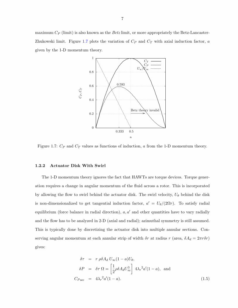
7
maximum C
P
(limit) is also known as the Betz limit, or more appropriately the Betz-Lancaster-
Zhukowski limit. Figure 1.7 plots the variation of C
P
and C
T
with axial induction factor, a
given by the 1-D momentum theory.
0
0.2
0.4
0.6
0.8
1
0.333 0.5
CP,C
T
a
0.593
Betz theory invalid
CT
CP
Uw/U∞
Figure 1.7: C
P
and C
T
values as functions of induction, a from the 1-D momentum theory.
1.2.2 Actuator Disk With Swirl
The 1-D momentum theory ignores the fact that HAWTs are torque devices. Torque gener-
ation requires a change in angular momentum of the fluid across a rotor. This is incorporated
by allowing the flow to swirl behind the actuator disk. The swirl velocity, U
✓
behind the disk
is non-dimensionalized to get tangential induction factor, a
0 = U
✓
/(2⌦r). To satisfy radial
equilibrium (force balance in radial direction), a, a
0 and other quantities have to vary radially
and the flow has to be analyzed in 2-D (axial and radial); azimuthal symmetry is still assumed.
This is typically done by discretizing the actuator disk into multiple annular sections. Con-
serving angular momentum at each annular strip of width �r at radius r (area, �Ad
= 2⇡r�r)
gives:
�⌧ = r ⇢�A
d
U1(1� a)U✓
,
�P = �⌧ ⌦ =12⇢�A
d
U
3
1
�4�
r
2
a
0(1� a), and
C
P
sec
= 4�r
2
a
0(1� a). (1.5)
8
0
0.2
0.4
0.6
0.8
1
0 5 10 15
a,a�
� r
aa�
(a) a, a0 as functions of �r
0
0.1
0.2
0.3
0.4
0.5
0.6
0 5 10 15
CP
�(b) CP
max
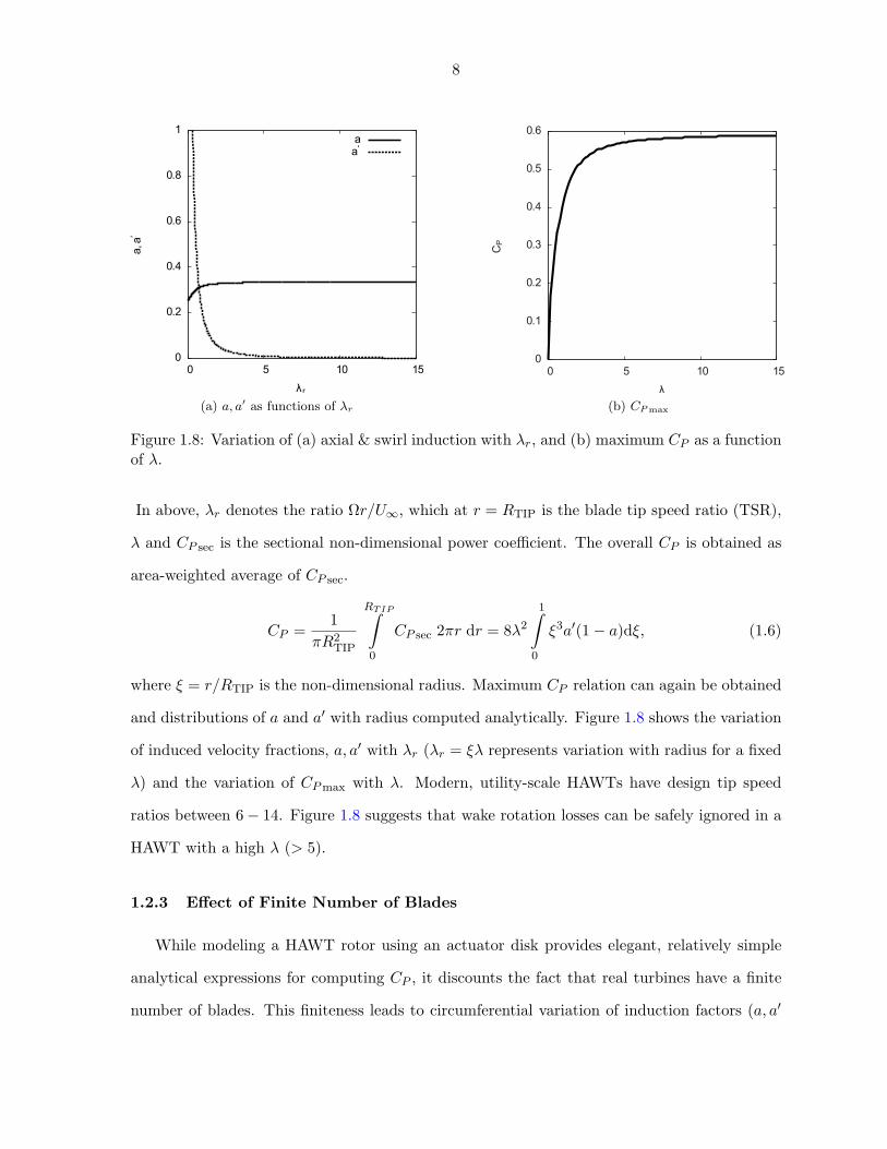
Figure 1.8: Variation of (a) axial & swirl induction with �r
, and (b) maximum C
P
as a functionof �.
In above, �r
denotes the ratio ⌦r/U1, which at r = R
TIP
is the blade tip speed ratio (TSR),
� and C
P
sec
is the sectional non-dimensional power coe�cient. The overall C
P
is obtained as
area-weighted average of C
P
sec
.
C
P
=1
⇡R
2
TIP
RTIPZ
0
C
P
sec
2⇡r dr = 8�2
1Z
0
⇠
3
a
0(1� a)d⇠, (1.6)
where ⇠ = r/R
TIP
is the non-dimensional radius. Maximum C
P
relation can again be obtained
and distributions of a and a
0 with radius computed analytically. Figure 1.8 shows the variation
of induced velocity fractions, a, a
0 with �r
(�r
= ⇠� represents variation with radius for a fixed
�) and the variation of C
P
max
with �. Modern, utility-scale HAWTs have design tip speed
ratios between 6� 14. Figure 1.8 suggests that wake rotation losses can be safely ignored in a
HAWT with a high � (> 5).
1.2.3 E↵ect of Finite Number of Blades
While modeling a HAWT rotor using an actuator disk provides elegant, relatively simple
analytical expressions for computing C
P
, it discounts the fact that real turbines have a finite
number of blades. This finiteness leads to circumferential variation of induction factors (a, a
0
9
are now functions of r and ✓), and this circumferential non-uniformity generates additional
losses.
In momentum-theory based approaches, the e↵ect of finite number of blades can be approx-
imately accounted for by hub/tip loss corrections. These corrections are specified as factors
that are multiplied with aerodynamic forces. These factors mimic the lift reduction due to in-
duction from trailing vorticity in a finite-span blade. Prandtl’s hub/tip loss model, for example
is widely used in HAWT aerodynamic analysis. In contrast, in models based on vortex theory,
each blade is represented by a line (or plane/array) of bound vortices and the wake by a helical
vortex sheet extending from the trailing edge of each blade to far enough downstream (Tre↵tz
plane). Induction is computed using the Biot-Savart’s law and aerodynamic forces on blades
are computed using the Kutta-Jukowski theorem [4].
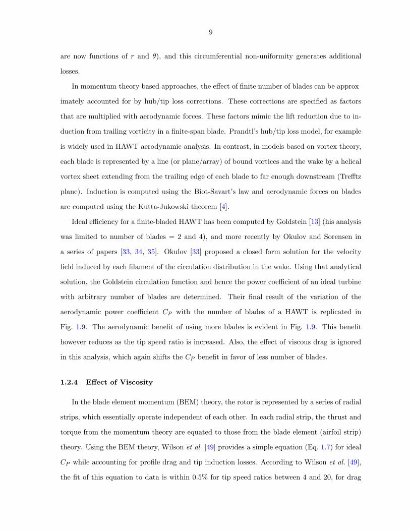
Ideal e�ciency for a finite-bladed HAWT has been computed by Goldstein [13] (his analysis
was limited to number of blades = 2 and 4), and more recently by Okulov and Sorensen in
a series of papers [33, 34, 35]. Okulov [33] proposed a closed form solution for the velocity
field induced by each filament of the circulation distribution in the wake. Using that analytical
solution, the Goldstein circulation function and hence the power coe�cient of an ideal turbine
with arbitrary number of blades are determined. Their final result of the variation of the
aerodynamic power coe�cient C
P
with the number of blades of a HAWT is replicated in
Fig. 1.9. The aerodynamic benefit of using more blades is evident in Fig. 1.9. This benefit
however reduces as the tip speed ratio is increased. Also, the e↵ect of viscous drag is ignored
in this analysis, which again shifts the C
P
benefit in favor of less number of blades.
1.2.4 E↵ect of Viscosity
In the blade element momentum (BEM) theory, the rotor is represented by a series of radial
strips, which essentially operate independent of each other. In each radial strip, the thrust and
torque from the momentum theory are equated to those from the blade element (airfoil strip)
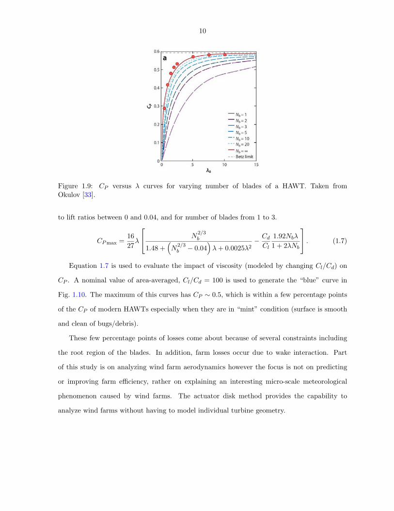
theory. Using the BEM theory, Wilson et al. [49] provides a simple equation (Eq. 1.7) for ideal
C
P
while accounting for profile drag and tip induction losses. According to Wilson et al. [49],
the fit of this equation to data is within 0.5% for tip speed ratios between 4 and 20, for drag
10
Figure 1.9: C
P
versus � curves for varying number of blades of a HAWT. Taken fromOkulov [33].
to lift ratios between 0 and 0.04, and for number of blades from 1 to 3.
C
P
max
=1627�
2
4 N
2/3
b
1.48 +⇣N
2/3
b
� 0.04⌘�+ 0.0025�2
� C
d
C
l
1.92N
b
�
1 + 2�N
b
3
5. (1.7)
Equation 1.7 is used to evaluate the impact of viscosity (modeled by changing C
l
/C
d
) on
C
P
. A nominal value of area-averaged, C
l
/C
d
= 100 is used to generate the “blue” curve in
Fig. 1.10. The maximum of this curves has C
P
⇠ 0.5, which is within a few percentage points
of the C
P
of modern HAWTs especially when they are in “mint” condition (surface is smooth
and clean of bugs/debris).
These few percentage points of losses come about because of several constraints including
the root region of the blades. In addition, farm losses occur due to wake interaction. Part
of this study is on analyzing wind farm aerodynamics however the focus is not on predicting
or improving farm e�ciency, rather on explaining an interesting micro-scale meteorological
phenomenon caused by wind farms. The actuator disk method provides the capability to
analyze wind farms without having to model individual turbine geometry.
11
Figure 1.10: Maximum possible C
P
with various approximations (Selvaraj et al. [42]).
1.3 Numerical modeling of wind turbine aerodynamics
The OpenFOAM software suite is chosen for numerical investigations of the two problems:
(1) DRWT aerodynamic analyses, and (2) modeling of surface flow convergence in wind farms.
OpenFOAM is essentially a group of C++ libraries used to create solvers. Some commonly
used numerical solvers for fluid flow simulations are provided in the software package. The
particular solver (with some additions and modifications) used in the present study is called
SimpleFOAM. The governing equations solved by the SimpleFOAM solver are the incompress-
ible RANS equations:
@u
i
@x
i
= 0, and, (1.8)
u
j
@u
i
@x
j
= �1⇢
@p
@x
i
� ⌫ @2
u
i
@x
j
2
�@u
0i
u
0j
@x
j
+f
i
⇢
. (1.9)
The Reynolds stress tensor, u
0i
u
0j
is modeled using eddy (“turbulent”) viscosity as ⌫t
@u
i
@x
j
. Tur-
bulent viscosity, ⌫t
is obtained using turbulent kinetic energy, k and dissipation, ✏, which are
themselves obtained by solving a transport equation for each. The term f
i
represents body
force per unit volume. A finite volume in the computational domain is defined (corresponding
to rotor swept area times small thickness) where body forces from equations 1.15 are applied to
12
model the e↵ect of the rotor. The magnitude of the body force and its direction are obtained
using the 2-D airfoil theory. By probing the CFD at the rotor disk, the local velocity is ob-
tained. Using the prescribed blade pitch and twist, �, the local angle of attack, ↵ to the airfoil
is obtained. Two-dimensional airfoil polars (Cl
� ↵ and C
d
� ↵ curves) combined with local
velocity and airfoil chord give the sectional lift and drag coe�cients, C
l
and C
d
(see Fig. 1.11).
Components of these forces (summed over all turbine blades) along the coordinate axes are
then used as body forces in the corresponding momentum equations.
1.3.1 Airfoil force distribution
Consider a 2-D airfoil at point P (r, ✓, 0) on a turbine rotating clockwise when observed from
a point upstream. In Fig. 1.11, the airfoil is assumed to be moving in the e
✓
direction. The
local flow velocity in the cylindrical coordinate system is (Vr
, V
✓
, V
z
). The flow velocity relative
to the blade is (Vr
, V
✓
�⌦r, V
z
). The airfoil stagger, ✓, and the flow angle, �, are measured from
the negative e
z
direction. The angle of attack, ↵, is the di↵erence between the airfoil stagger
and the flow angle.
� = tan�1
✓⌦r � V
✓
V
z
◆and, (1.10)
↵ = ✓ � �. (1.11)
The non-dimensional lift and drag forces, C
l
and C
d
, are decomposed as thrust and torque
forces, C
TF and C
⌧F
e
z
: Thrust force coe�cient = C
l
sin�+ C
d
cos� = C
TF and, (1.12)
e
✓
: Torque force coe�cient = C
l
cos�� C
d
sin� = C
⌧F . (1.13)
The above non-dimensional force coe�cients are for an annulus with a single blade. The
net force on the annular disk with B number of blades between r � dr/2 and r + dr/2 is given
by
13
e
z
: dT
F
= B
1
2
�(⌦r � V
✓
)2 + V
2
z
�c⇥ dr| {z }
dS
C
TF and, (1.14)
e
✓
: d⌧
F
= B
1
2
�(⌦r � V
✓
)2 + V
2
z
�c⇥ dr| {z }
dS
C
⌧F . (1.15)
These forces are implemented as body forces (fi
) in the RANS equations 1.9. To avoid
a sudden jump in the forces at the location of the actuator disk, which is known to cause
numerical instability, a smooth Gaussian distribution (along e
z
) for these forces is used rather
than a uniform (rectangular) distribution with discontinuities.
Figure 1.11: Airfoil
1.3.2 Gaussian Distribution of forces
The forces are distributed over a volume and a Gaussian distribution is applied along the
flow direction following Mikkelsen [30]. The magnitude of the body force term for each cell
is determined by the Gaussian distribution. The disk has a thickness of �x. Each disk is
separated into annuli of thickness dr along the radial direction. The axisymmetric cross section
of annulus is shown in figure 1.12.
At a radius r
m
, say the volume density of the thrust force is ⇢TF (r, z). Then
14
Figure 1.12: Axisymmetric cross section of the annulus at radius r
m
dT
F
=
�z2Z
��z2
⇢
TF (r, z)⇥ (2⇡r
m
) dr ⇥ dz =B
2
⇣V
2
z
+ (⌦r � V
✓
)2⌘
c dr C
TF and,
�z2Z
��z2
⇢
TF (r, z)⇥ dz =B
4⇡r
m
⇣V
2
z
+ (⌦r � V
✓
)2⌘
cC
TF .
The distribution fuction ⇢TF (r, z) may use a uniform distribution or a Gaussian distribution
along z. For uniform distribution of forces
⇢
T
(r, z) =B
4⇡r
m
�z
⇥�(⌦r � V
✓
)2 + V
2
z
�cC
T
.
For Gaussian distribution of forces
⇢
T
(r, z) =A(r)
�
p2⇡
exp{� (z�z
0
)
2
2�
2
}
erf
h�z
2
p2�
i,
where the error function, erf(z) = 2p⇡
zR
0
e
�t
2
dt.
The integral of density function,
�z2Z
��z2
⇢
T
(r, z) = A =)
0
BB@*
�z2Z
��z2
A
�
p2⇡
exp{�(z � z
0
)2
2�2
}dz = A erf
�z
2p
2�
�1
CCA
15
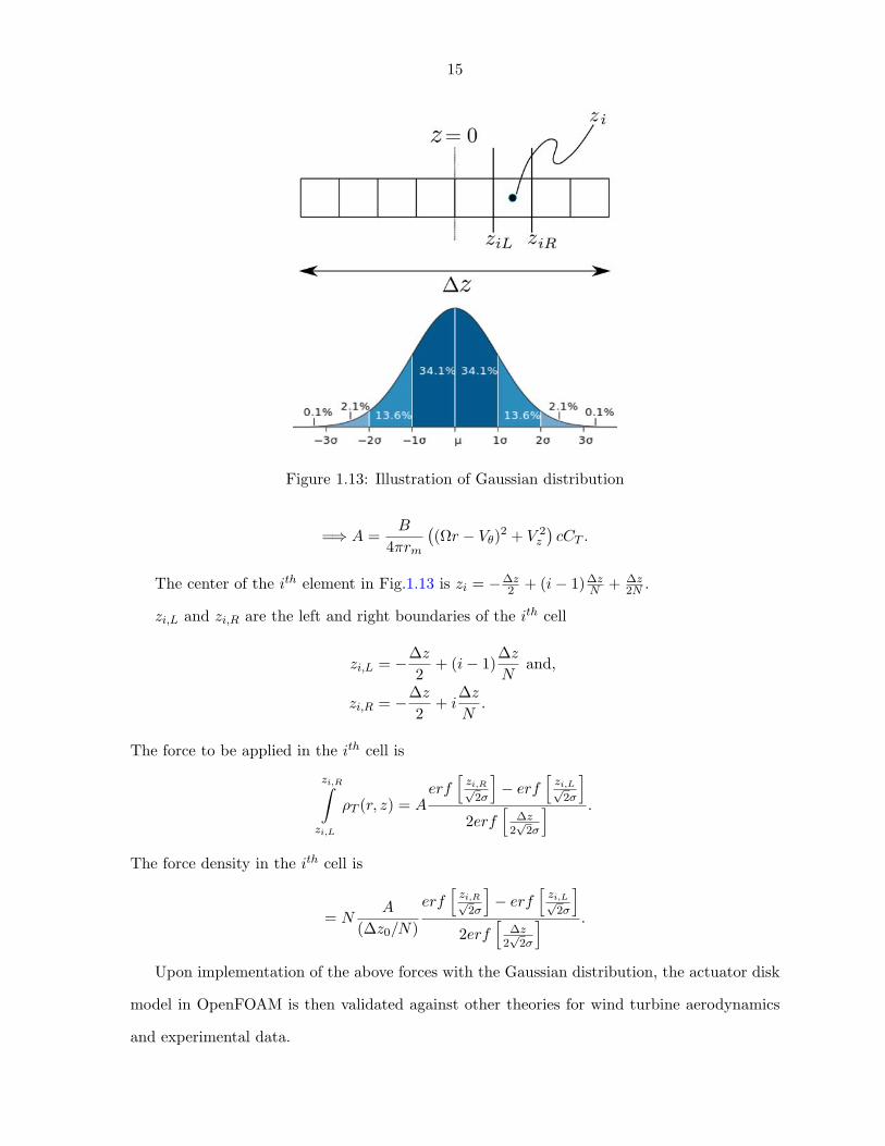
Figure 1.13: Illustration of Gaussian distribution
=) A =B
4⇡r
m
�(⌦r � V
✓
)2 + V
2
z
�cC
T
.
The center of the i
th element in Fig.1.13 is z
i
= ��z
2
+ (i� 1)�z
N
+ �z
2N
.
z
i,L
and z
i,R
are the left and right boundaries of the i
th cell
z
i,L
= ��z
2+ (i� 1)
�z
N
and,
z
i,R
= ��z
2+ i
�z
N
.
The force to be applied in the i
th cell is
zi,RZ
zi,L
⇢
T
(r, z) = A
erf
hzi,Rp
2�
i� erf
hzi,Lp
2�
i
2erf
h�z
2
p2�
i.
The force density in the i
th cell is
= N
A
(�z
0
/N)
erf
hzi,Rp
2�
i� erf
hzi,Lp
2�
i
2erf
h�z
2
p2�
i.
Upon implementation of the above forces with the Gaussian distribution, the actuator disk
model in OpenFOAM is then validated against other theories for wind turbine aerodynamics
and experimental data.
16
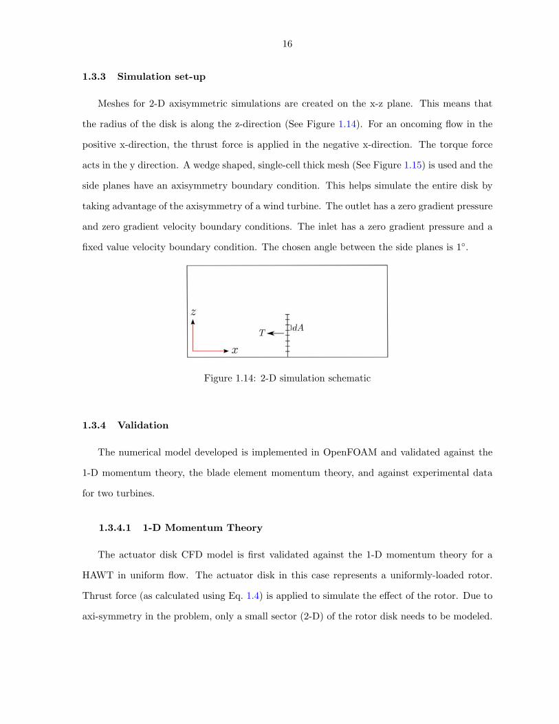
1.3.3 Simulation set-up
Meshes for 2-D axisymmetric simulations are created on the x-z plane. This means that
the radius of the disk is along the z-direction (See Figure 1.14). For an oncoming flow in the
positive x-direction, the thrust force is applied in the negative x-direction. The torque force
acts in the y direction. A wedge shaped, single-cell thick mesh (See Figure 1.15) is used and the
side planes have an axisymmetry boundary condition. This helps simulate the entire disk by
taking advantage of the axisymmetry of a wind turbine. The outlet has a zero gradient pressure
and zero gradient velocity boundary conditions. The inlet has a zero gradient pressure and a
fixed value velocity boundary condition. The chosen angle between the side planes is 1�.
Figure 1.14: 2-D simulation schematic
1.3.4 Validation
The numerical model developed is implemented in OpenFOAM and validated against the
1-D momentum theory, the blade element momentum theory, and against experimental data
for two turbines.
1.3.4.1 1-D Momentum Theory
The actuator disk CFD model is first validated against the 1-D momentum theory for a
HAWT in uniform flow. The actuator disk in this case represents a uniformly-loaded rotor.
Thrust force (as calculated using Eq. 1.4) is applied to simulate the e↵ect of the rotor. Due to
axi-symmetry in the problem, only a small sector (2-D) of the rotor disk needs to be modeled.
17
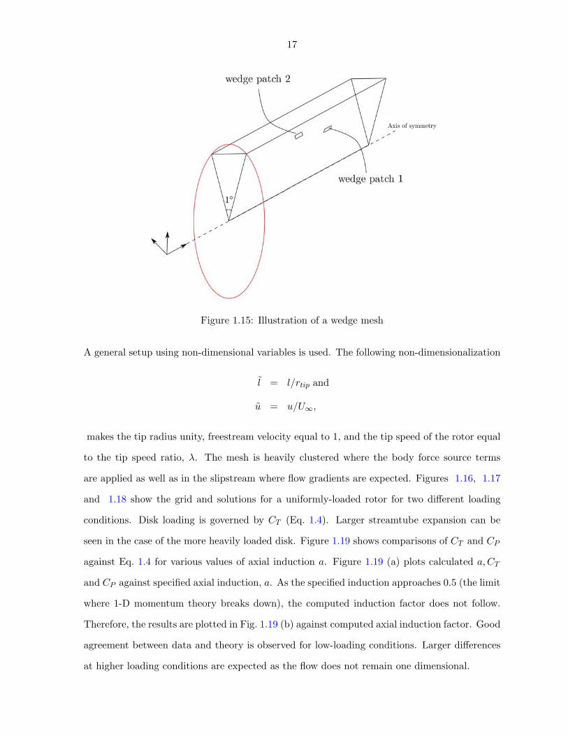
Figure 1.15: Illustration of a wedge mesh
A general setup using non-dimensional variables is used. The following non-dimensionalization
l = l/r
tip
and
u = u/U1,
makes the tip radius unity, freestream velocity equal to 1, and the tip speed of the rotor equal
to the tip speed ratio, �. The mesh is heavily clustered where the body force source terms
are applied as well as in the slipstream where flow gradients are expected. Figures 1.16, 1.17
and 1.18 show the grid and solutions for a uniformly-loaded rotor for two di↵erent loading
conditions. Disk loading is governed by C
T
(Eq. 1.4). Larger streamtube expansion can be
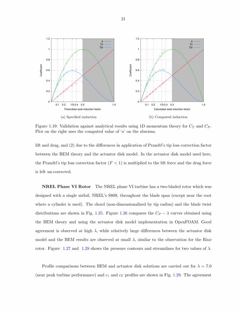
seen in the case of the more heavily loaded disk. Figure 1.19 shows comparisons of C
T
and C
P
against Eq. 1.4 for various values of axial induction a. Figure 1.19 (a) plots calculated a, C
T
and C
P
against specified axial induction, a. As the specified induction approaches 0.5 (the limit
where 1-D momentum theory breaks down), the computed induction factor does not follow.
Therefore, the results are plotted in Fig. 1.19 (b) against computed axial induction factor. Good
agreement between data and theory is observed for low-loading conditions. Larger di↵erences
at higher loading conditions are expected as the flow does not remain one dimensional.
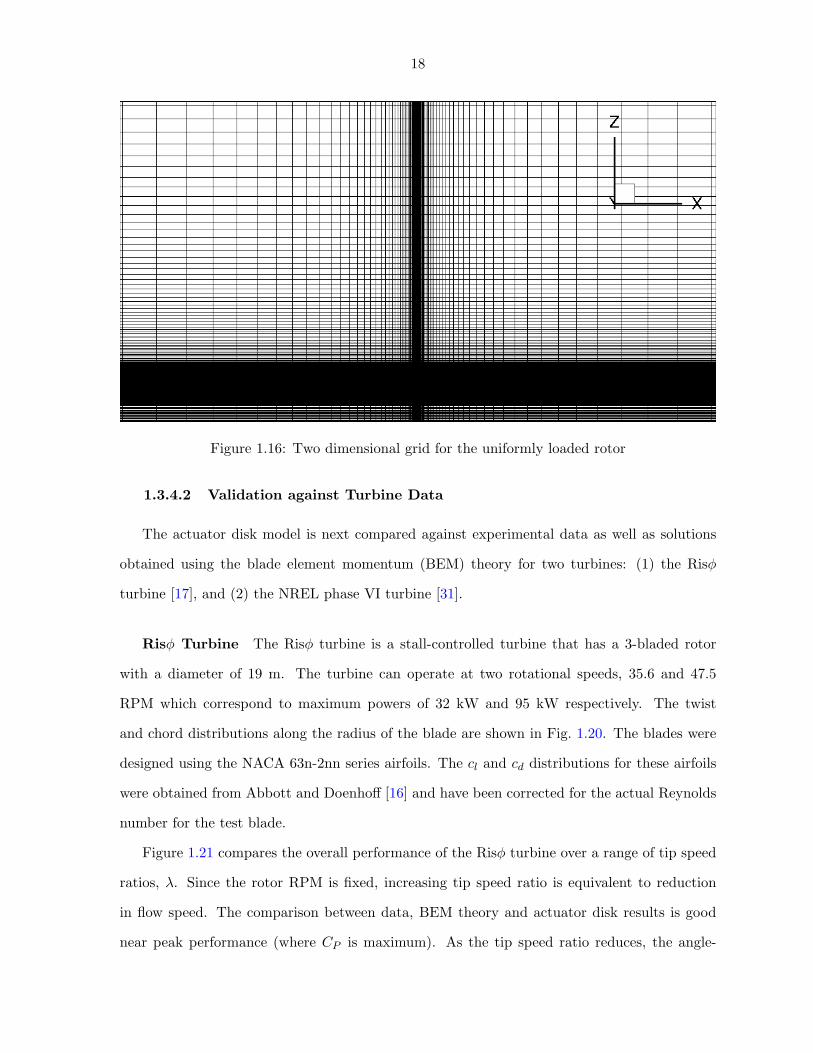
18
Figure 1.16: Two dimensional grid for the uniformly loaded rotor
1.3.4.2 Validation against Turbine Data
The actuator disk model is next compared against experimental data as well as solutions
obtained using the blade element momentum (BEM) theory for two turbines: (1) the Ris�
turbine [17], and (2) the NREL phase VI turbine [31].
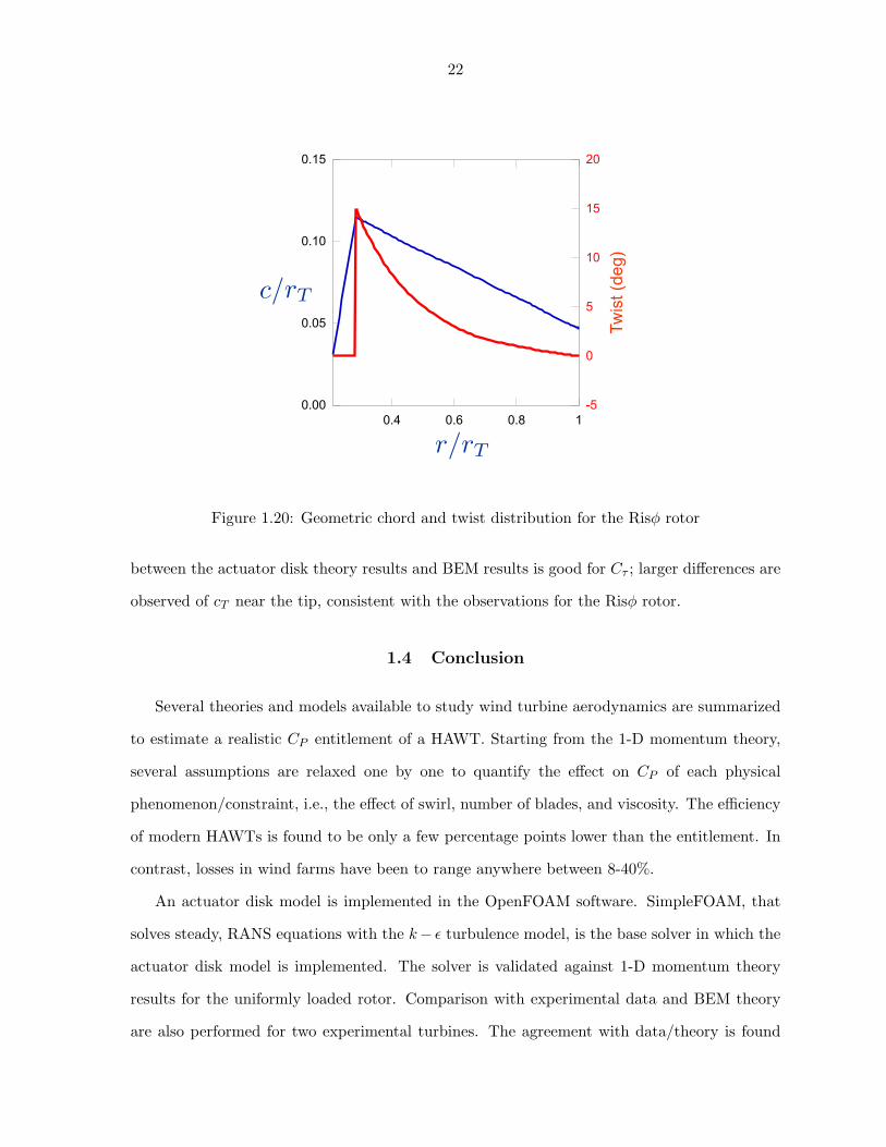
Ris� Turbine The Ris� turbine is a stall-controlled turbine that has a 3-bladed rotor
with a diameter of 19 m. The turbine can operate at two rotational speeds, 35.6 and 47.5
RPM which correspond to maximum powers of 32 kW and 95 kW respectively. The twist
and chord distributions along the radius of the blade are shown in Fig. 1.20. The blades were
designed using the NACA 63n-2nn series airfoils. The c
l
and c
d
distributions for these airfoils
were obtained from Abbott and Doenho↵ [16] and have been corrected for the actual Reynolds
number for the test blade.
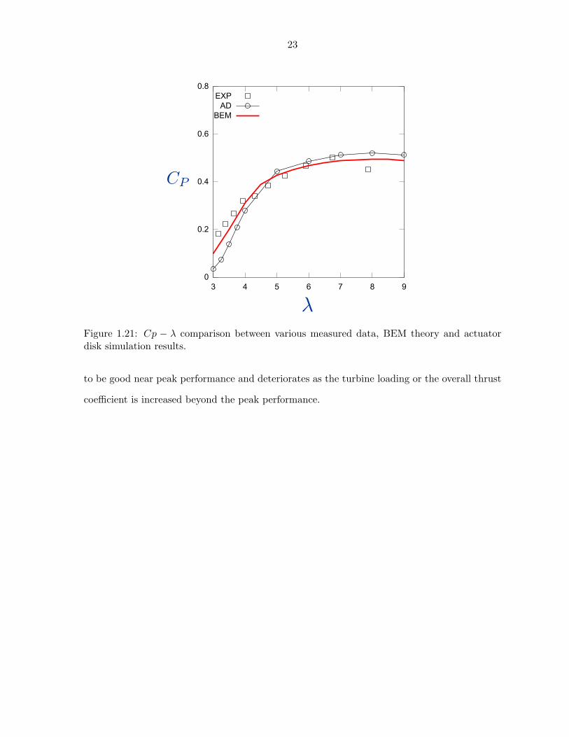
Figure 1.21 compares the overall performance of the Ris� turbine over a range of tip speed
ratios, �. Since the rotor RPM is fixed, increasing tip speed ratio is equivalent to reduction
in flow speed. The comparison between data, BEM theory and actuator disk results is good
near peak performance (where C
P
is maximum). As the tip speed ratio reduces, the angle-
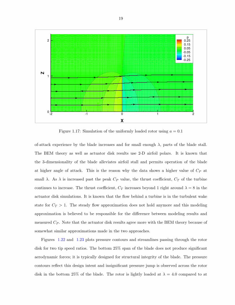
19
X
Z
-2 -1 0 1 20
1
2p
0.250.150.05
-0.05-0.15-0.25
Figure 1.17: Simulation of the uniformly loaded rotor using a = 0.1
of-attack experience by the blade increases and for small enough �, parts of the blade stall.
The BEM theory as well as actuator disk results use 2-D airfoil polars. It is known that
the 3-dimensionality of the blade alleviates airfoil stall and permits operation of the blade
at higher angle of attack. This is the reason why the data shows a higher value of C
P
at
small �. As � is increased past the peak C
P
value, the thrust coe�cient, C
T
of the turbine
continues to increase. The thrust coe�cient, C
T
increases beyond 1 right around � = 8 in the
actuator disk simulations. It is known that the flow behind a turbine is in the turbulent wake
state for C
T
> 1. The steady flow approximation does not hold anymore and this modeling
approximation is believed to be responsible for the di↵erence between modeling results and
measured C
P
. Note that the actuator disk results agree more with the BEM theory because of
somewhat similar approximations made in the two approaches.
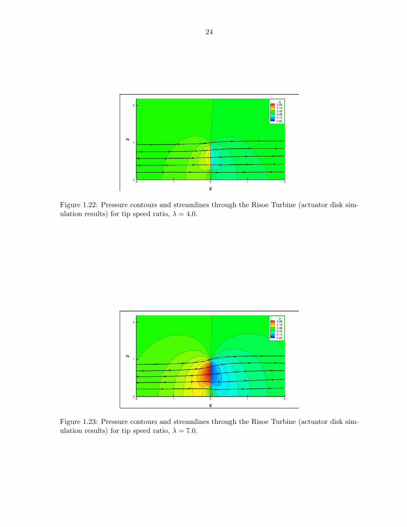
Figures 1.22 and 1.23 plots pressure contours and streamlines passing through the rotor
disk for two tip speed ratios. The bottom 25% span of the blade does not produce significant
aerodynamic forces; it is typically designed for structural integrity of the blade. The pressure
contours reflect this design intent and insignificant pressure jump is observed across the rotor
disk in the bottom 25% of the blade. The rotor is lightly loaded at � = 4.0 compared to at
20
X
Z
-2 -1 0 1 20
1
2p
0.250.150.05
-0.05-0.15-0.25
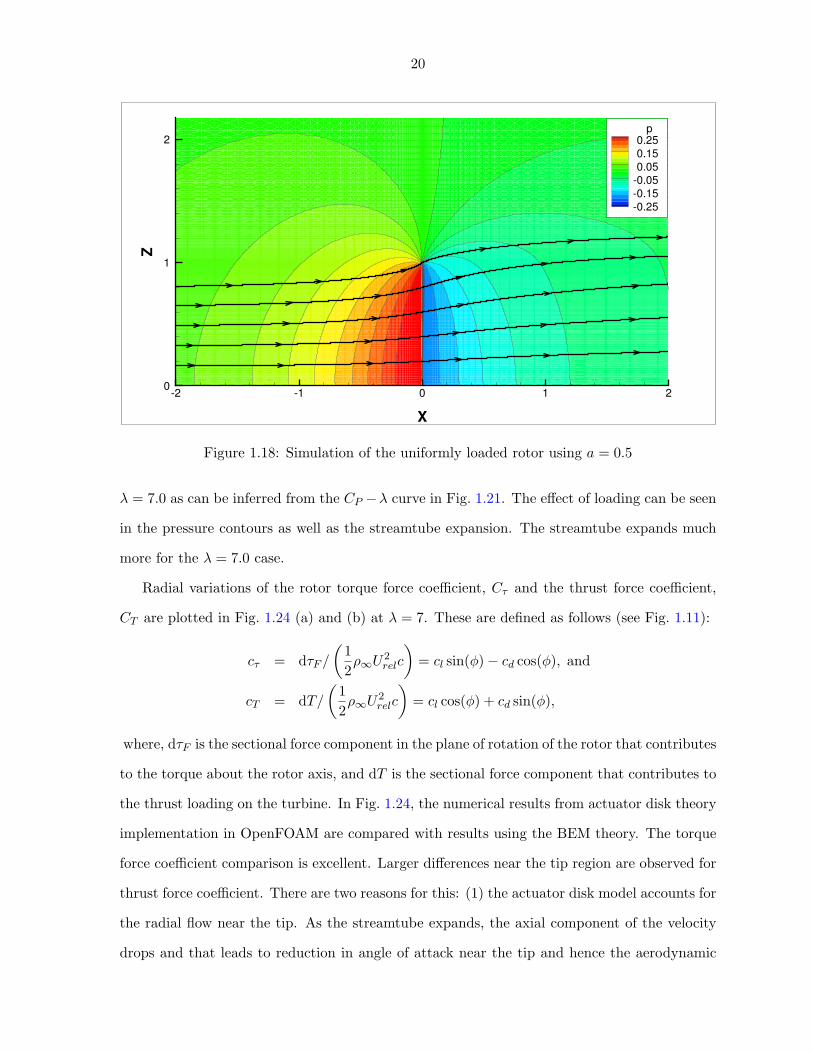
Figure 1.18: Simulation of the uniformly loaded rotor using a = 0.5
� = 7.0 as can be inferred from the C
P
�� curve in Fig. 1.21. The e↵ect of loading can be seen
in the pressure contours as well as the streamtube expansion. The streamtube expands much
more for the � = 7.0 case.
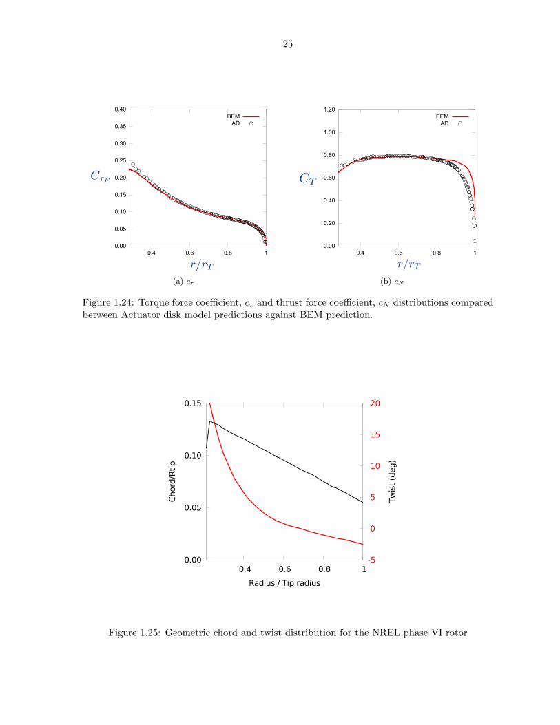
Radial variations of the rotor torque force coe�cient, C
⌧
and the thrust force coe�cient,
C
T
are plotted in Fig. 1.24 (a) and (b) at � = 7. These are defined as follows (see Fig. 1.11):
c
⌧
= d⌧F
/
✓12⇢1U
2
rel
c
◆= c
l
sin(�)� c
d
cos(�), and
c
T
= dT/
✓12⇢1U
2
rel
c
◆= c
l
cos(�) + c
d
sin(�),
where, d⌧F
is the sectional force component in the plane of rotation of the rotor that contributes
to the torque about the rotor axis, and dT is the sectional force component that contributes to
the thrust loading on the turbine. In Fig. 1.24, the numerical results from actuator disk theory
implementation in OpenFOAM are compared with results using the BEM theory. The torque
force coe�cient comparison is excellent. Larger di↵erences near the tip region are observed for
thrust force coe�cient. There are two reasons for this: (1) the actuator disk model accounts for
the radial flow near the tip. As the streamtube expands, the axial component of the velocity
drops and that leads to reduction in angle of attack near the tip and hence the aerodynamic
21
0
0.2
0.4
0.6
0.8
1
1.2
0.1 0.2 1/3 0.4 0.5 1.0
Coe
ffici
ent
Prescribed axial induction factor
aCtCp
(a) Specified induction
0
0.2
0.4
0.6
0.8
1
1.2
0.1 0.2 1/3 0.4 0.5 1.0
Coe
ffici
ent
Calculated axial induction factor
aCtCp
(b) Computed induction
Figure 1.19: Validation against analytical results using 1D momentum theory for C
T
and C
P
.Plot on the right uses the computed value of ‘a’ on the abscissa.
lift and drag, and (2) due to the di↵erences in application of Prandtl’s tip loss correction factor
between the BEM theory and the actuator disk model. In the actuator disk model used here,
the Prandtl’s tip loss correction factor (F < 1) is multiplied to the lift force and the drag force
is left un-corrected.
NREL Phase VI Rotor The NREL phase VI turbine has a two-bladed rotor which was
designed with a single airfoil, NREL’s S809, throughout the blade span (except near the root
where a cylinder is used). The chord (non-dimensionalized by tip radius) and the blade twist
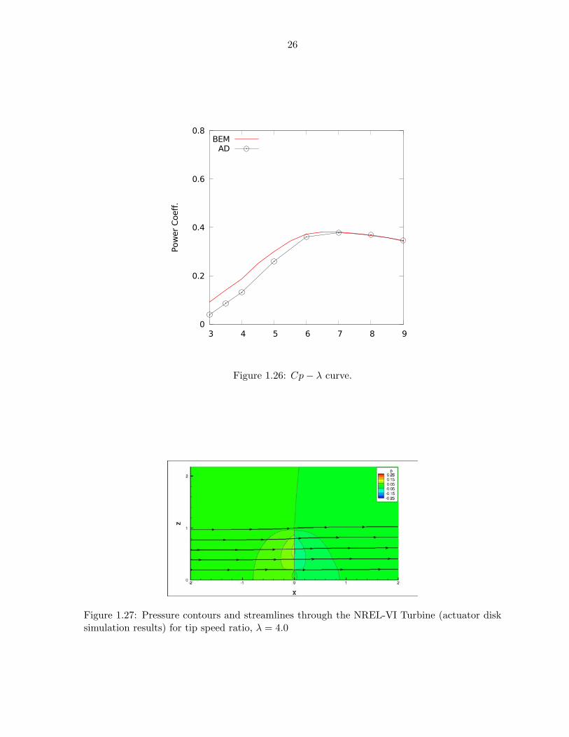
distributions are shown in Fig. 1.25. Figure 1.26 compares the C
P
� � curves obtained using
the BEM theory and using the actuator disk model implementation in OpenFOAM. Good
agreement is observed at high �, while relatively large di↵erences between the actuator disk
model and the BEM results are observed at small �, similar to the observation for the Ris�
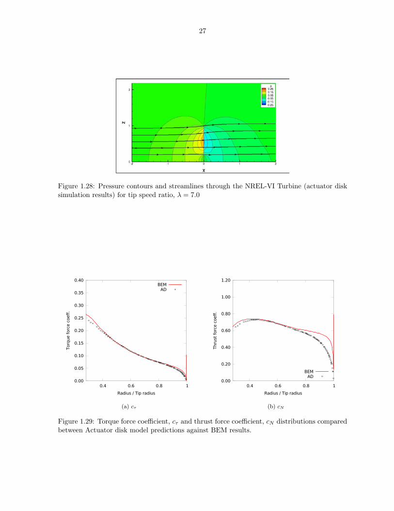
rotor. Figure 1.27 and 1.28 shows the pressure contours and streamlines for two values of �.
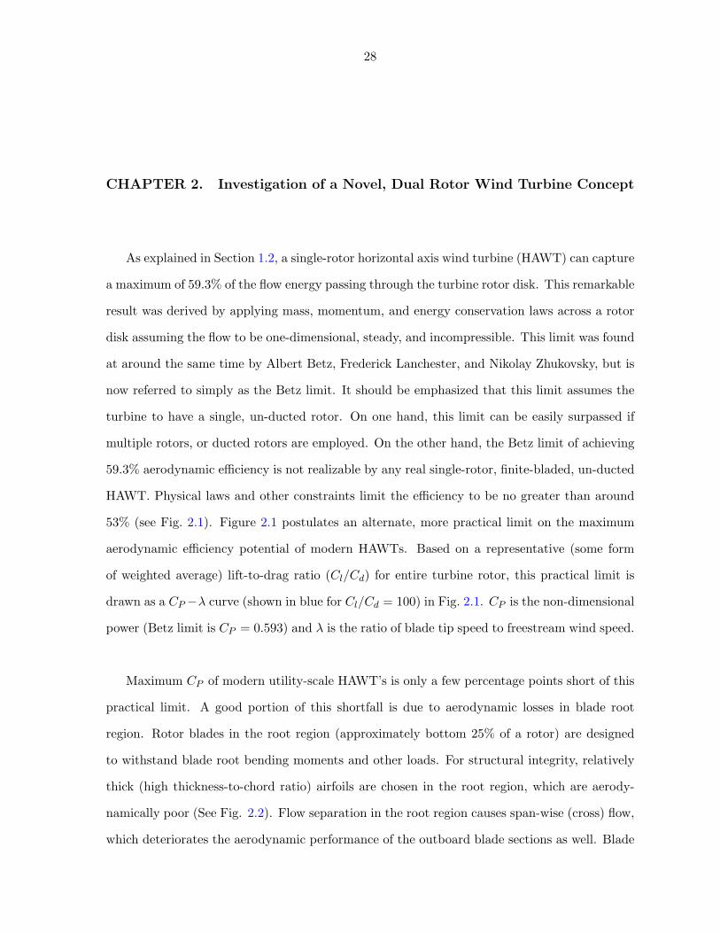
Profile comparisons between BEM and actuator disk solutions are carried out for � = 7.0
(near peak turbine performance) and c
⌧
and c
T
profiles are shown in Fig. 1.29. The agreement
22
Figure 1.20: Geometric chord and twist distribution for the Ris� rotor
between the actuator disk theory results and BEM results is good for C
⌧
; larger di↵erences are
observed of c
T
near the tip, consistent with the observations for the Ris� rotor.
1.4 Conclusion
Several theories and models available to study wind turbine aerodynamics are summarized
to estimate a realistic C
P
entitlement of a HAWT. Starting from the 1-D momentum theory,
several assumptions are relaxed one by one to quantify the e↵ect on C
P
of each physical
phenomenon/constraint, i.e., the e↵ect of swirl, number of blades, and viscosity. The e�ciency
of modern HAWTs is found to be only a few percentage points lower than the entitlement. In
contrast, losses in wind farms have been to range anywhere between 8-40%.
An actuator disk model is implemented in the OpenFOAM software. SimpleFOAM, that
solves steady, RANS equations with the k� ✏ turbulence model, is the base solver in which the
actuator disk model is implemented. The solver is validated against 1-D momentum theory
results for the uniformly loaded rotor. Comparison with experimental data and BEM theory
are also performed for two experimental turbines. The agreement with data/theory is found
23
Figure 1.21: Cp � � comparison between various measured data, BEM theory and actuatordisk simulation results.
to be good near peak performance and deteriorates as the turbine loading or the overall thrust
coe�cient is increased beyond the peak performance.
24
Figure 1.22: Pressure contours and streamlines through the Risoe Turbine (actuator disk sim-ulation results) for tip speed ratio, � = 4.0.
Figure 1.23: Pressure contours and streamlines through the Risoe Turbine (actuator disk sim-ulation results) for tip speed ratio, � = 7.0.
25
(a) c⌧
(b) cN
Figure 1.24: Torque force coe�cient, c
⌧
and thrust force coe�cient, c
N
distributions comparedbetween Actuator disk model predictions against BEM prediction.
0.00
0.05
0.10
0.15
0.4 0.6 0.8 1-5
0
5
10
15
20
Chord
/Rti
p
Tw
ist
(deg)
Radius / Tip radius
Figure 1.25: Geometric chord and twist distribution for the NREL phase VI rotor
26
0
0.2
0.4
0.6
0.8
3 4 5 6 7 8 9
Pow
er
Coeff
.
BEMAD
Figure 1.26: Cp� � curve.
Figure 1.27: Pressure contours and streamlines through the NREL-VI Turbine (actuator disksimulation results) for tip speed ratio, � = 4.0
27
Figure 1.28: Pressure contours and streamlines through the NREL-VI Turbine (actuator disksimulation results) for tip speed ratio, � = 7.0
0.00
0.05
0.10
0.15
0.20
0.25
0.30
0.35
0.40
0.4 0.6 0.8 1
Torq
ue f
orc
e c
oeff
.
Radius / Tip radius
BEMAD
(a) c⌧
0.00
0.20
0.40
0.60
0.80
1.00
1.20
0.4 0.6 0.8 1
Thru
st f
orc
e c
oeff
.
Radius / Tip radius
BEMAD
(b) cN
Figure 1.29: Torque force coe�cient, c
⌧
and thrust force coe�cient, c
N
distributions comparedbetween Actuator disk model predictions against BEM results.
28
CHAPTER 2. Investigation of a Novel, Dual Rotor Wind Turbine Concept
As explained in Section 1.2, a single-rotor horizontal axis wind turbine (HAWT) can capture
a maximum of 59.3% of the flow energy passing through the turbine rotor disk. This remarkable
result was derived by applying mass, momentum, and energy conservation laws across a rotor
disk assuming the flow to be one-dimensional, steady, and incompressible. This limit was found
at around the same time by Albert Betz, Frederick Lanchester, and Nikolay Zhukovsky, but is
now referred to simply as the Betz limit. It should be emphasized that this limit assumes the
turbine to have a single, un-ducted rotor. On one hand, this limit can be easily surpassed if
multiple rotors, or ducted rotors are employed. On the other hand, the Betz limit of achieving
59.3% aerodynamic e�ciency is not realizable by any real single-rotor, finite-bladed, un-ducted
HAWT. Physical laws and other constraints limit the e�ciency to be no greater than around
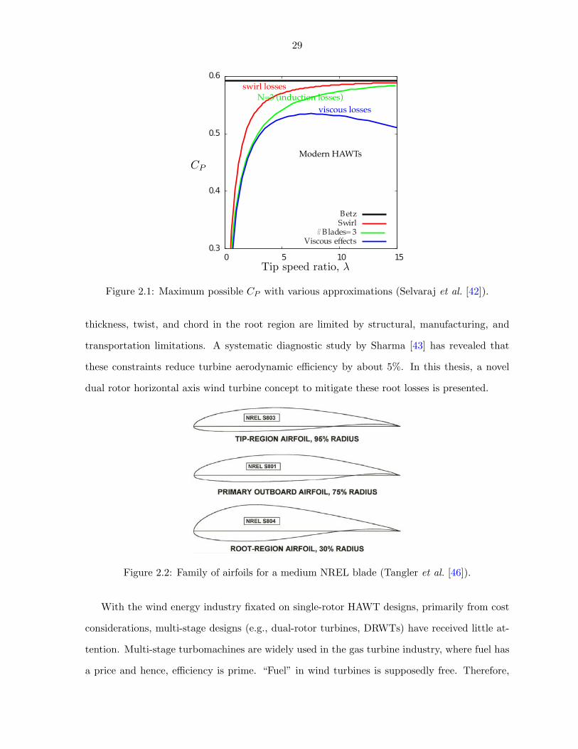
53% (see Fig. 2.1). Figure 2.1 postulates an alternate, more practical limit on the maximum
aerodynamic e�ciency potential of modern HAWTs. Based on a representative (some form
of weighted average) lift-to-drag ratio (Cl
/C
d
) for entire turbine rotor, this practical limit is
drawn as a C
P
�� curve (shown in blue for C
l
/C
d
= 100) in Fig. 2.1. C
P
is the non-dimensional
power (Betz limit is C
P
= 0.593) and � is the ratio of blade tip speed to freestream wind speed.
Maximum C
P
of modern utility-scale HAWT’s is only a few percentage points short of this
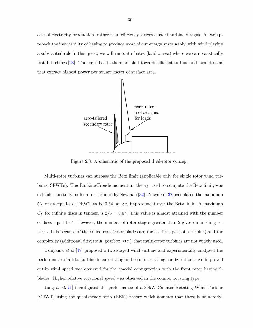
practical limit. A good portion of this shortfall is due to aerodynamic losses in blade root
region. Rotor blades in the root region (approximately bottom 25% of a rotor) are designed
to withstand blade root bending moments and other loads. For structural integrity, relatively
thick (high thickness-to-chord ratio) airfoils are chosen in the root region, which are aerody-
namically poor (See Fig. 2.2). Flow separation in the root region causes span-wise (cross) flow,
which deteriorates the aerodynamic performance of the outboard blade sections as well. Blade
29
Figure 2.1: Maximum possible C
P
with various approximations (Selvaraj et al. [42]).
thickness, twist, and chord in the root region are limited by structural, manufacturing, and
transportation limitations. A systematic diagnostic study by Sharma [43] has revealed that
these constraints reduce turbine aerodynamic e�ciency by about 5%. In this thesis, a novel
dual rotor horizontal axis wind turbine concept to mitigate these root losses is presented.
Figure 2.2: Family of airfoils for a medium NREL blade (Tangler et al. [46]).
With the wind energy industry fixated on single-rotor HAWT designs, primarily from cost
considerations, multi-stage designs (e.g., dual-rotor turbines, DRWTs) have received little at-
tention. Multi-stage turbomachines are widely used in the gas turbine industry, where fuel has
a price and hence, e�ciency is prime. “Fuel” in wind turbines is supposedly free. Therefore,
30
cost of electricity production, rather than e�ciency, drives current turbine designs. As we ap-
proach the inevitability of having to produce most of our energy sustainably, with wind playing
a substantial role in this quest, we will run out of sites (land or sea) where we can realistically
install turbines [28]. The focus has to therefore shift towards e�cient turbine and farm designs
that extract highest power per square meter of surface area.
Figure 2.3: A schematic of the proposed dual-rotor concept.
Multi-rotor turbines can surpass the Betz limit (applicable only for single rotor wind tur-
bines, SRWTs). The Rankine-Froude momentum theory, used to compute the Betz limit, was
extended to study multi-rotor turbines by Newman [32]. Newman [32] calculated the maximum
C
P
of an equal-size DRWT to be 0.64, an 8% improvement over the Betz limit. A maximum
C
P
for infinite discs in tandem is 2/3 = 0.67. This value is almost attained with the number
of discs equal to 4. However, the number of rotor stages greater than 2 gives diminishing re-
turns. It is because of the added cost (rotor blades are the costliest part of a turbine) and the
complexity (additional drivetrain, gearbox, etc.) that multi-rotor turbines are not widely used.
Ushiyama et al.[47] proposed a two staged wind turbine and experimentally analyzed the
performance of a trial turbine in co-rotating and counter-rotating configurations. An improved
cut-in wind speed was observed for the coaxial configuration with the front rotor having 2-
blades. Higher relative rotational speed was observed in the counter rotating type.
Jung et al.[21] investigated the performance of a 30kW Counter Rotating Wind Turbine
(CRWT) using the quasi-steady strip (BEM) theory which assumes that there is no aerody-
31
namic interference between the main and the auxiliary rotors. The optimum values for distance
between the rotors and the size of the auxiliary rotor were found to be one half of the auxiliary
rotor diameter and one half of the main rotor diameter respectively.
Kanemoto and Galal [22] proposed a wind turbine generator with tandem rotors and double
rotational armatures. The larger front rotor and the smaller rear rotor drive the inner and outer
armatures respectively to keep the rotational torque counter-balanced. The setup enables higher
output than the conventional wind turbine and constant output in the rated operating mode
without the need to use the brake or pitch control mechanisms.
Lee et al. [26] considered e↵ects of solidity when comparing counter rotating wind turbines
(CRWT) to single rotors. As most comparisons from previous researchers only consider CRWT
and a single rotor with half solidity as the CRWT, Lee et al.[26] felt it was not a fair comparison.
A 30% increase in power was observed when comparing the CRWT configuration to the single
rotor with half solidity. A 5% decrease in power was observed when comparing the CRWT
configuration with a single rotor having equal solidity.
Lee et al. [27] investigated e↵ects of design parameters such as combination of pitch angles,
rotating speed ratio and radius di↵erence on a CRWT. It was found that when the radius
of the front rotor was about 0.8 times the radius of the rear rotor, the power coe�cient was
maximum. The maximum power is also obtained when the rotating speed of the rear rotor is
reduced to recover the angle of the relative wind for maximum performance of the rear rotor.
Kumar et al. [24] used the commercial CFD software Fluent to compare the performance of
CRWT and Single Rotor Wind Turbine (SRWT). They further investigated the values for the
optimum axial distance between the rotors in a CRWT as done previously by Jung et al.[21]
and found that the power increase is about 10% for a wind velocity of 10 m/s with an axial
distance of 0.65D (D is the diameter of the primary rotor).
Yuan et al. [51] conducted an experimental study to investigate the power production per-
formance and flow characteristics of two wind turbines in tandem in co-rotating and counter-
rotating configurations. The upwind turbine generates an azimuthal velocity component in it’s
wake which has di↵erent e↵ects on the downstream turbines depending on whether they are
in the co-rotating or in the counter-rotating configuration. The azimuthal velocity component
32
reduces the e↵ective angle of attack for the downstream rotor in the co-rotating configuration
and hence the lift is reduced whereas for the counter-rotating configuration, the e↵ective angle
of attack is increased due to the azimuthal e↵ect and the lift produced is higher. A 17% increase
in power output was observed in the counter-rotating configuration compared to co-rotating
configuration.
Windpower Engineering & Development has developed a co-axial, twin-rotor turbine with
the objective of harvesting more energy at lower wind speeds. They use two identical rotors
connected by one shaft to a variable-speed generator. Enercon also has a patent [50] on a
dual-rotor concept similar to the one proposed here, however the patent is focused on growing
rotor radius rather than reducing losses.
A dual-rotor turbine concept (see Fig. 2.3) is proposed and investigated here. In this dual-
rotor concept, a smaller, aerodynamically tailored, secondary co-axial rotor is placed ahead of
the main rotor. None of the DRWT articles referenced above focus on what is targeted here with
the proposed DRWT concept. The objectives of the DRWT concept are: (1) reduce root losses,
and (2) reduce wake losses in a wind farm through enhanced wake mixing. The first goal targets
improving isolated turbine e�ciency through the use of aerodynamically optimized secondary
rotor. The second goal targets e�ciency improvement at wind-farm scale by (a) tailoring
rotor wake shear, and (b) by exploiting dynamic interaction between vortices from main and
secondary rotors of a DRWT. This thesis focuses only on the first of the two objectives.
2.1 Numerical Simulations using RANS CFD
The RANS method described in Chapter 1 can be directly used to simulate dual-rotor wind
turbine aerodynamics. The two rotors of a DRWT are modeled as two di↵erent, independent
single-rotor turbines. It should be borne in mind that the two rotors of a DRWT are in close
proximity, with a consequence that the potential fields of one rotor can a↵ect the other. Such
potential field interaction is not modeled here due to parameterization of rotors by actuator
disk/line methods. While the potential field interaction cannot be completely ignored, a con-
ceptual evaluation of the DRWT concept, such as proposed here, can be conducted with this
simplification.
33
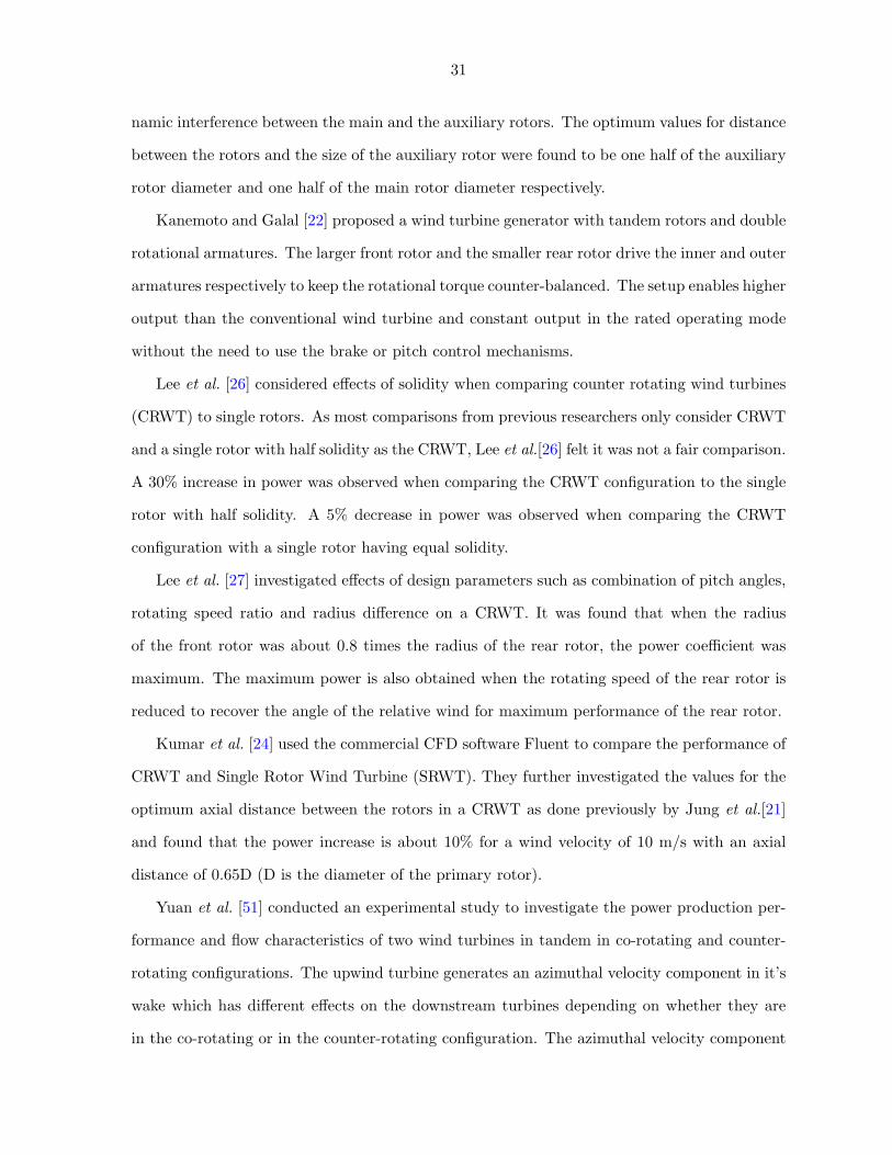
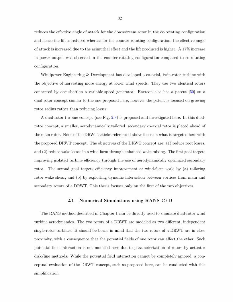
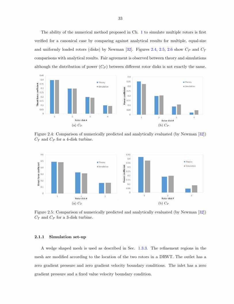
The ability of the numerical method proposed in Ch. 1 to simulate multiple rotors is first
verified for a canonical case by comparing against analytical results for multiple, equal-size
and uniformly loaded rotors (disks) by Newman [32]. Figures 2.4, 2.5, 2.6 show C
P
and C
T
comparisons with analytical results. Fair agreement is observed between theory and simulations
although the distribution of power (CP
) between di↵erent rotor disks is not exactly the same.
(a) CT (b) CP
Figure 2.4: Comparison of numerically predicted and analytically evaluated (by Newman [32])C
T
and C
P
for a 4-disk turbine.
(a) CT (b) CP
Figure 2.5: Comparison of numerically predicted and analytically evaluated (by Newman [32])C
T
and C
P
for a 3-disk turbine.
2.1.1 Simulation set-up
A wedge shaped mesh is used as described in Sec. 1.3.3. The refinement regions in the
mesh are modified according to the location of the two rotors in a DRWT. The outlet has a
zero gradient pressure and zero gradient velocity boundary conditions. The inlet has a zero
gradient pressure and a fixed value velocity boundary condition.
34
(a) CT (b) CP
Figure 2.6: Comparison of numerically predicted and analytically evaluated (by Newman [32])C
T
and C
P
for a 2-disk turbine.
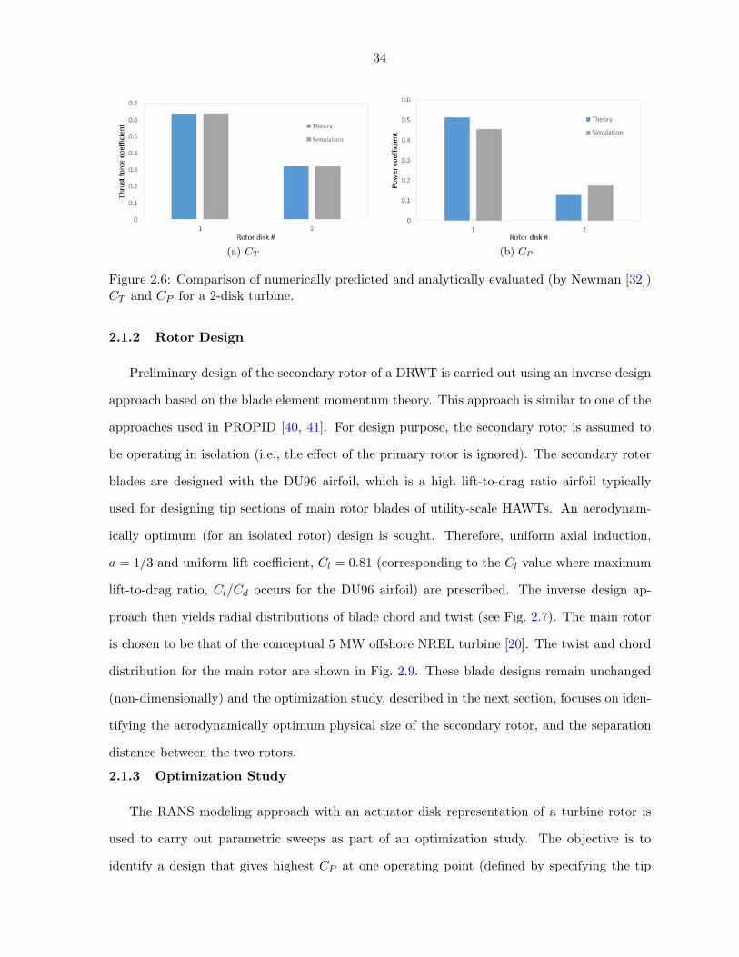
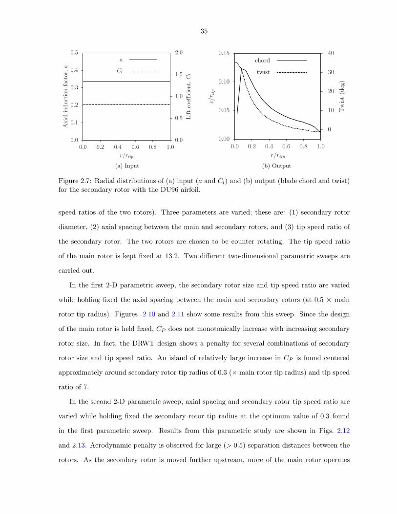
2.1.2 Rotor Design
Preliminary design of the secondary rotor of a DRWT is carried out using an inverse design
approach based on the blade element momentum theory. This approach is similar to one of the
approaches used in PROPID [40, 41]. For design purpose, the secondary rotor is assumed to
be operating in isolation (i.e., the e↵ect of the primary rotor is ignored). The secondary rotor
blades are designed with the DU96 airfoil, which is a high lift-to-drag ratio airfoil typically
used for designing tip sections of main rotor blades of utility-scale HAWTs. An aerodynam-
ically optimum (for an isolated rotor) design is sought. Therefore, uniform axial induction,
a = 1/3 and uniform lift coe�cient, C
l
= 0.81 (corresponding to the C
l
value where maximum
lift-to-drag ratio, C
l
/C
d
occurs for the DU96 airfoil) are prescribed. The inverse design ap-
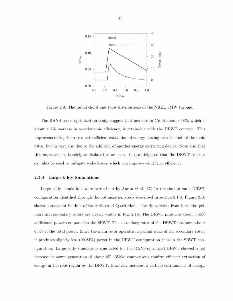
proach then yields radial distributions of blade chord and twist (see Fig. 2.7). The main rotor
is chosen to be that of the conceptual 5 MW o↵shore NREL turbine [20]. The twist and chord
distribution for the main rotor are shown in Fig. 2.9. These blade designs remain unchanged
(non-dimensionally) and the optimization study, described in the next section, focuses on iden-
tifying the aerodynamically optimum physical size of the secondary rotor, and the separation
distance between the two rotors.
2.1.3 Optimization Study
The RANS modeling approach with an actuator disk representation of a turbine rotor is
used to carry out parametric sweeps as part of an optimization study. The objective is to
identify a design that gives highest C
P
at one operating point (defined by specifying the tip
35
0.0
0.1
0.2
0.3
0.4
0.5
0.0 0.2 0.4 0.6 0.8 1.00.0
0.5
1.0
1.5
2.0
Axi
alin
duct
ion
fact
or,a
Lift
coe�
cien
t,C
l
r/rtip
a
Cl
(a) Input
0.00
0.05
0.10
0.15
0.0 0.2 0.4 0.6 0.8 1.0
0
10
20
30
40
c/r t
ip
Twist(deg)
r/rtip
chord
twist
(b) Output
Figure 2.7: Radial distributions of (a) input (a and C
l
) and (b) output (blade chord and twist)for the secondary rotor with the DU96 airfoil.
speed ratios of the two rotors). Three parameters are varied; these are: (1) secondary rotor
diameter, (2) axial spacing between the main and secondary rotors, and (3) tip speed ratio of
the secondary rotor. The two rotors are chosen to be counter rotating. The tip speed ratio
of the main rotor is kept fixed at 13.2. Two di↵erent two-dimensional parametric sweeps are
carried out.
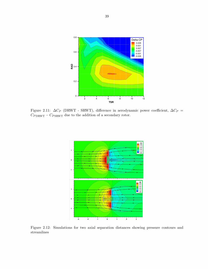
In the first 2-D parametric sweep, the secondary rotor size and tip speed ratio are varied
while holding fixed the axial spacing between the main and secondary rotors (at 0.5 ⇥ main
rotor tip radius). Figures 2.10 and 2.11 show some results from this sweep. Since the design
of the main rotor is held fixed, C
P
does not monotonically increase with increasing secondary
rotor size. In fact, the DRWT design shows a penalty for several combinations of secondary
rotor size and tip speed ratio. An island of relatively large increase in C
P
is found centered
approximately around secondary rotor tip radius of 0.3 (⇥ main rotor tip radius) and tip speed
ratio of 7.
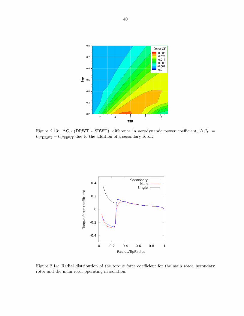
In the second 2-D parametric sweep, axial spacing and secondary rotor tip speed ratio are
varied while holding fixed the secondary rotor tip radius at the optimum value of 0.3 found
in the first parametric sweep. Results from this parametric study are shown in Figs. 2.12
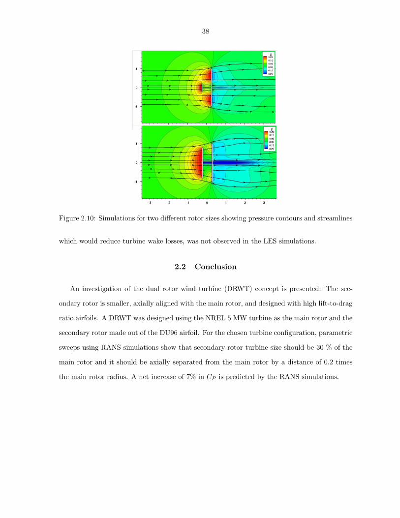
and 2.13. Aerodynamic penalty is observed for large (> 0.5) separation distances between the
rotors. As the secondary rotor is moved further upstream, more of the main rotor operates
36
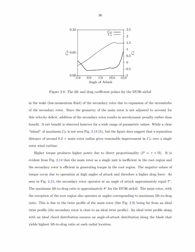
Figure 2.8: The lift and drag coe�cient polars for the DU96 airfoil
in the wake (low-momentum fluid) of the secondary rotor due to expansion of the streamtube
of the secondary rotor. Since the geometry of the main rotor is not adjusted to account for
this velocity deficit, addition of the secondary rotor results in aerodynamic penalty rather than
benefit. A net benefit is observed however for a wide range of parametric values. While a clear
“island” of maximum C
P
is not seen Fig. 2.13 (b), but the figure does suggest that a separation
distance of around 0.2 ⇥ main rotor radius gives reasonable improvement in C
P
over a single
rotor wind turbine.
Higher torque produces higher power due to direct proportionality (P = ⌧ ⇥ ⌦). It is
evident from Fig. 2.14 that the main rotor as a single unit is ine�cient in the root region and
the secondary rotor is e�cient in generating torque in the root region. The negative values of
torque occur due to operation at high angles of attack and therefore a higher drag force. As
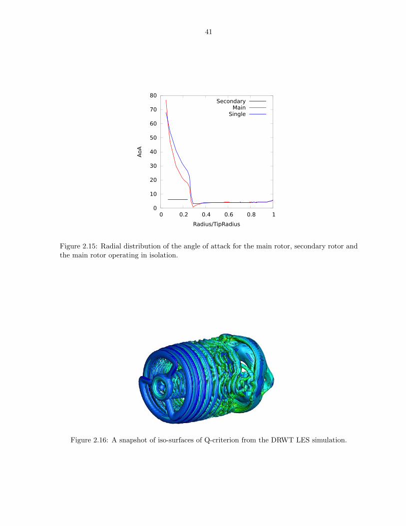
seen in Fig. 2.15, the secondary rotor operates at an angle of attack approximately equal 7�.
The maximum lift-to-drag ratio is approximately 8� for the DU96 airfoil. The main rotor, with
the exception of the root region also operates at angles corresponding to maximum lift-to-drag
ratio. This is due to the twist profile of the main rotor (See Fig. 2.9) being far from an ideal
twist profile (the secondary rotor is close to an ideal twist profile). An ideal twist profile along
with an ideal chord distribution ensures an angle-of-attack distribution along the blade that
yields highest lift-to-drag ratio at each radial location.
37
Figure 2.9: The radial chord and twist distributions of the NREL 5MW turbine.
The RANS based optimization study suggest that increase in C
P
of about 0.035, which is
about a 7% increase in aerodynamic e�ciency, is attainable with the DRWT concept. This
improvement is primarily due to e�cient extraction of energy flowing near the hub of the main
rotor, but in part also due to the addition of another energy extracting device. Note also that
this improvement is solely on isolated rotor basis. It is anticipated that the DRWT concept
can also be used to mitigate wake losses, which can improve wind farm e�ciency.
2.1.4 Large Eddy Simulations
Large eddy simulations were carried out by Aaron et al. [37] for the the optimum DRWT
configuration identified through the optimization study described in section 2.1.3. Figure 2.16
shows a snapshot in time of iso-surfaces of Q-criterion. The tip vortices from both the pri-
mary and secondary rotors are clearly visible in Fig. 2.16. The DRWT produces about 5.66%
additional power compared to the SRWT. The secondary rotor of the DRWT produces about
6.3% of the total power. Since the main rotor operates in partial wake of the secondary rotor,
it produces slightly less (99.24%) power in the DRWT configuration than in the SRWT con-
figuration. Large eddy simulations conducted for the RANS-optimized DRWT showed a net
increase in power generation of about 6%. Wake comparisons confirm e�cient extraction of
energy in the root region by the DRWT. However, increase in vertical entrainment of energy,
38
Figure 2.10: Simulations for two di↵erent rotor sizes showing pressure contours and streamlines
which would reduce turbine wake losses, was not observed in the LES simulations.
2.2 Conclusion
An investigation of the dual rotor wind turbine (DRWT) concept is presented. The sec-
ondary rotor is smaller, axially aligned with the main rotor, and designed with high lift-to-drag
ratio airfoils. A DRWT was designed using the NREL 5 MW turbine as the main rotor and the
secondary rotor made out of the DU96 airfoil. For the chosen turbine configuration, parametric
sweeps using RANS simulations show that secondary rotor turbine size should be 30 % of the
main rotor and it should be axially separated from the main rotor by a distance of 0.2 times
the main rotor radius. A net increase of 7% in C
P
is predicted by the RANS simulations.
39
TSR
RA
D
2 4 6 8 10 12
0
0.2
0.4
0.6
0.8
Delta CP
0.035
0.021
0.007
-0.007
-0.021
-0.035
Figure 2.11: �C
P
(DRWT - SRWT), di↵erence in aerodynamic power coe�cient, �C
P
=C
P
DRWT
� C
P
SRWT
due to the addition of a secondary rotor.
Figure 2.12: Simulations for two axial separation distances showing pressure contours andstreamlines
40
TSR
Se
p
2 4 6 8 10
0.2
0.3
0.4
0.5
0.6
0.7
0.8
Delta CP
0.035
0.026
0.017
0.008
-0.001
-0.01
Figure 2.13: �C
P
(DRWT - SRWT), di↵erence in aerodynamic power coe�cient, �C
P
=C
P
DRWT
� C
P
SRWT
due to the addition of a secondary rotor.
Figure 2.14: Radial distribution of the torque force coe�cient for the main rotor, secondaryrotor and the main rotor operating in isolation.
41
Figure 2.15: Radial distribution of the angle of attack for the main rotor, secondary rotor andthe main rotor operating in isolation.
Figure 2.16: A snapshot of iso-surfaces of Q-criterion from the DRWT LES simulation.
42
CHAPTER 3. Wind Farm Aerodynamics
Utility scale turbines are deployed in clusters called wind farms. It is now recognized
by the wind energy community that these turbines cannot be studied and/or optimized as
if operating in isolation. Aerodynamic interaction between turbines in wind farms results in
significant energy loss that ranges anywhere between 8-40% [5]. The primary mechanism of
this energy loss is ingestion (by downstream turbines) of reduced-momentum air present in the
wakes of upstream turbines. The range of this loss is exceptionally wide because of its strong
dependence on farm location, layout (micro-siting), and atmospheric stability. Highest losses
have been observed in o↵shore turbines when turbine rows are aligned with wind direction, are
closely spaced, and when atmospheric flow is stably stratified [6, 14]). In comparison to the
large body of work devoted to measuring and predicting wake losses, relatively little research
has focused on reducing wake losses. For HAWTs, Corten and Lindenburg [9] have developed
a method of farm control in which windward turbines are deliberately yawed (skewed) with
respect to wind direction. The concept is to use the lateral force (generated by deliberate
yawing of windward turbines) to divert the flow away from downstream turbines. The degree
of yaw is determined based on wind and turbine row alignment.
Wind turbine and wind farm aerodynamics can be modeled with a spectrum of tools ranging
from analytical models to high fidelity computational fluid dynamics (CFD) models [36, 8].
Vermeer et al. [48] and Sanderse et al. [39] provide excellent reviews of the state-of-the-art
numerical methods to analyze wind turbine and wind farm aerodynamics. CFD modeling of
wind turbines and turbine arrays can be classified into two categories based on whether or
not rotor geometry is resolved. In investigations of turbine wake evolution (far wake) or wind
farm aerodynamics, resolving rotor blades is arguably unnecessary. The e↵ect of rotors on wake
flows in such simulations is represented through sources in the momentum equation. This source
43
representation can be in the form of actuator disk, line, or surface. Sørensen and Shen [44]
and Mikkelsen [30] provide a nice summary of such methods. Besides rotor parameterization,
numerical solution fidelity can vary considerably based on which temporal and spatial scales
are resolved.
Several wake models have also been suggested by Vermeer et al. [48], Lissaman [38], Larsen
et al. [25], Katic et al. [23] and Ainslie [2] for the use of analysis of the performance of wind
farms.
Mandas et al. [29] used the commercial CFD code Fluent to solve 3-D turbulent-steady,
incompressible, RANS equations to study wind turbine aerodynamics. The BEM method was
used in the design process of a blade where the active part of the blade is extended to the hub
(i.e without a cylindrical connection to the hub). Di↵erent aspects of the HAWT flow-field
such as the hub, tip, near and far wakes were resolved despite the di↵erent scales. To study
aerodynamic characteristics in a wind farm while resolving individual turbine geometry such as
done in this paper would be computationally very expensive. Hence the actuator disk method
described in Sec. 1.3 is used for wind farm aerodynamic analyses presented here.
Frandsen et al. [12] proposed a wind farm model that encompasses the flow characteristics
of very large wind farms in a realistic and consistent manner with appropriate experimental
calibration.
Johnson and Thomas [19] proposed that coordinated control of the turbines located near
each other by intelligent selection of the axial induction factor can increase the energy captured
by the array of turbines.
Ammara et al. [3] developed a viscous three dimensional/actuator disk method for the
aerodynamic analysis of wind farms. Analysis was performed on a two row periodic wind farm
and the results showed positive interference e↵ects. It was concluded that an appropriately
designed wind farm can be as e�cient as those of a sparse arrangement.
There has been some previous work analyzing performance of turbines and attempts at
mitigating wake losses in a wind farm as mentioned above. However, there has been no compu-
tational investigation to verify the phenomenon of flow convergence introduced in Sec. 1, which
is the primary focus of this thesis.
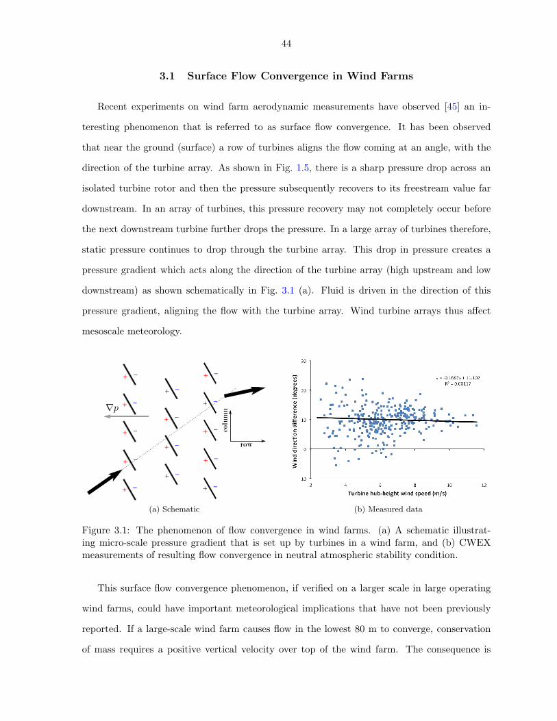
44
3.1 Surface Flow Convergence in Wind Farms
Recent experiments on wind farm aerodynamic measurements have observed [45] an in-
teresting phenomenon that is referred to as surface flow convergence. It has been observed
that near the ground (surface) a row of turbines aligns the flow coming at an angle, with the
direction of the turbine array. As shown in Fig. 1.5, there is a sharp pressure drop across an
isolated turbine rotor and then the pressure subsequently recovers to its freestream value far
downstream. In an array of turbines, this pressure recovery may not completely occur before
the next downstream turbine further drops the pressure. In a large array of turbines therefore,
static pressure continues to drop through the turbine array. This drop in pressure creates a
pressure gradient which acts along the direction of the turbine array (high upstream and low
downstream) as shown schematically in Fig. 3.1 (a). Fluid is driven in the direction of this
pressure gradient, aligning the flow with the turbine array. Wind turbine arrays thus a↵ect
mesoscale meteorology.
(a) Schematic (b) Measured data
Figure 3.1: The phenomenon of flow convergence in wind farms. (a) A schematic illustrat-ing micro-scale pressure gradient that is set up by turbines in a wind farm, and (b) CWEXmeasurements of resulting flow convergence in neutral atmospheric stability condition.
This surface flow convergence phenomenon, if verified on a larger scale in large operating
wind farms, could have important meteorological implications that have not been previously
reported. If a large-scale wind farm causes flow in the lowest 80 m to converge, conservation
of mass requires a positive vertical velocity over top of the wind farm. The consequence is
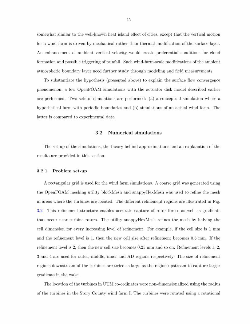
45
somewhat similar to the well-known heat island e↵ect of cities, except that the vertical motion
for a wind farm is driven by mechanical rather than thermal modification of the surface layer.
An enhancement of ambient vertical velocity would create preferential conditions for cloud
formation and possible triggering of rainfall. Such wind-farm-scale modifications of the ambient
atmospheric boundary layer need further study through modeling and field measurements.
To substantiate the hypothesis (presented above) to explain the surface flow convergence
phenomenon, a few OpenFOAM simulations with the actuator disk model described earlier
are performed. Two sets of simulations are performed: (a) a conceptual simulation where a
hypothetical farm with periodic boundaries and (b) simulations of an actual wind farm. The
latter is compared to experimental data.
3.2 Numerical simulations
The set-up of the simulations, the theory behind approximations and an explanation of the
results are provided in this section.
3.2.1 Problem set-up
A rectangular grid is used for the wind farm simulations. A coarse grid was generated using
the OpenFOAM meshing utility blockMesh and snappyHexMesh was used to refine the mesh
in areas where the turbines are located. The di↵erent refinement regions are illustrated in Fig.
3.2. This refinement structure enables accurate capture of rotor forces as well as gradients
that occur near turbine rotors. The utility snappyHexMesh refines the mesh by halving the
cell dimension for every increasing level of refinement. For example, if the cell size is 1 mm
and the refinement level is 1, then the new cell size after refinement becomes 0.5 mm. If the
refinement level is 2, then the new cell size becomes 0.25 mm and so on. Refinement levels 1, 2,
3 and 4 are used for outer, middle, inner and AD regions respectively. The size of refinement
regions downstream of the turbines are twice as large as the region upstream to capture larger
gradients in the wake.
The location of the turbines in UTM co-ordinates were non-dimensionalized using the radius
of the turbines in the Story County wind farm I. The turbines were rotated using a rotational
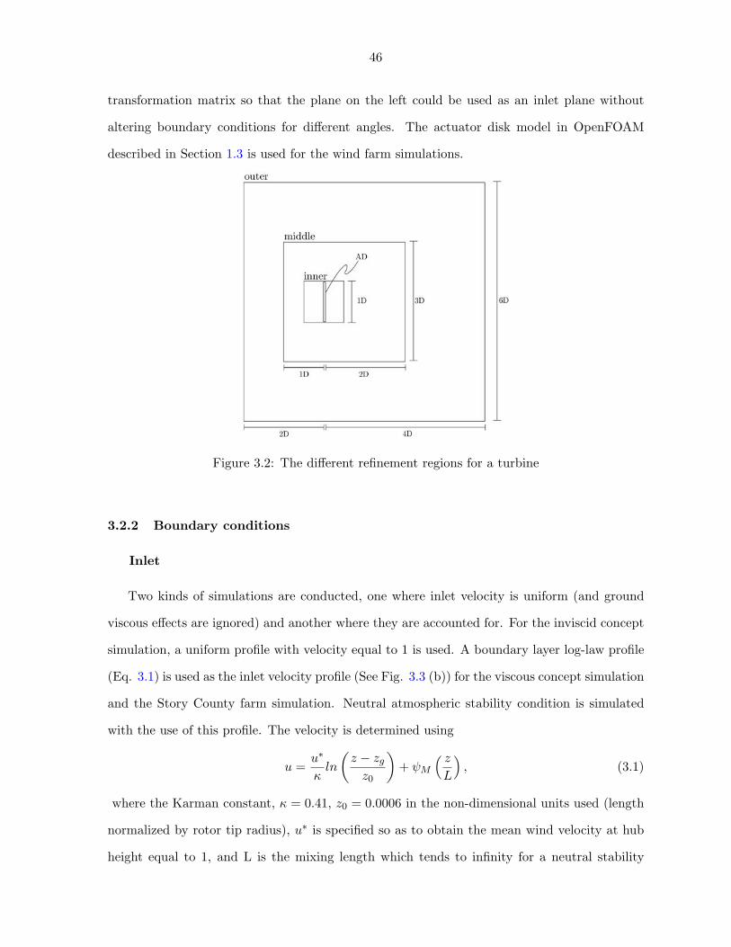
46
transformation matrix so that the plane on the left could be used as an inlet plane without
altering boundary conditions for di↵erent angles. The actuator disk model in OpenFOAM
described in Section 1.3 is used for the wind farm simulations.
Figure 3.2: The di↵erent refinement regions for a turbine
3.2.2 Boundary conditions
Inlet
Two kinds of simulations are conducted, one where inlet velocity is uniform (and ground
viscous e↵ects are ignored) and another where they are accounted for. For the inviscid concept
simulation, a uniform profile with velocity equal to 1 is used. A boundary layer log-law profile
(Eq. 3.1) is used as the inlet velocity profile (See Fig. 3.3 (b)) for the viscous concept simulation
and the Story County farm simulation. Neutral atmospheric stability condition is simulated
with the use of this profile. The velocity is determined using
u =u
⇤
ln
✓z � z
g
z
0
◆+
M
⇣z
L
⌘, (3.1)
where the Karman constant, = 0.41, z
0
= 0.0006 in the non-dimensional units used (length
normalized by rotor tip radius), u
⇤ is specified so as to obtain the mean wind velocity at hub
height equal to 1, and L is the mixing length which tends to infinity for a neutral stability
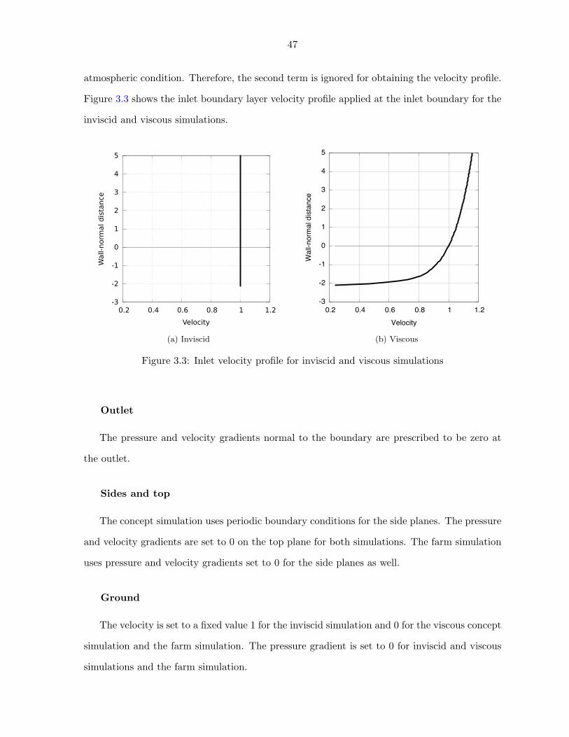
47
atmospheric condition. Therefore, the second term is ignored for obtaining the velocity profile.
Figure 3.3 shows the inlet boundary layer velocity profile applied at the inlet boundary for the
inviscid and viscous simulations.
(a) Inviscid
-3
-2
-1
0
1
2
3
4
5
0.2 0.4 0.6 0.8 1 1.2W
all-n
orm
al d
ista
nce
Velocity
(b) Viscous
Figure 3.3: Inlet velocity profile for inviscid and viscous simulations
Outlet
The pressure and velocity gradients normal to the boundary are prescribed to be zero at
the outlet.
Sides and top
The concept simulation uses periodic boundary conditions for the side planes. The pressure
and velocity gradients are set to 0 on the top plane for both simulations. The farm simulation
uses pressure and velocity gradients set to 0 for the side planes as well.
Ground
The velocity is set to a fixed value 1 for the inviscid simulation and 0 for the viscous concept
simulation and the farm simulation. The pressure gradient is set to 0 for inviscid and viscous
simulations and the farm simulation.
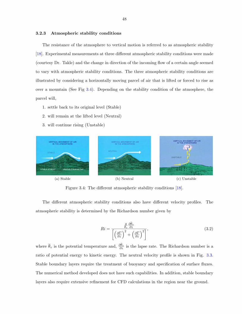
48
3.2.3 Atmospheric stability conditions
The resistance of the atmosphere to vertical motion is referred to as atmospheric stability
[18]. Experimental measurements at three di↵erent atmospheric stability conditions were made
(courtesy Dr. Takle) and the change in direction of the incoming flow of a certain angle seemed
to vary with atmospheric stability conditions. The three atmospheric stability conditions are
illustrated by considering a horizontally moving parcel of air that is lifted or forced to rise as
over a mountain (See Fig 3.4). Depending on the stability condition of the atmosphere, the
parcel will,
1. settle back to its original level (Stable)
2. will remain at the lifted level (Neutral)
3. will continue rising (Unstable)
(a) Stable (b) Neutral (c) Unstable
Figure 3.4: The di↵erent atmospheric stability conditions [18].
The di↵erent atmospheric stability conditions also have di↵erent velocity profiles. The
atmospheric stability is determined by the Richardson number given by
Ri =g
✓v
@✓v@z⇣
@U
@z
⌘2
+⇣
@V
@z
⌘2
�, (3.2)
where ✓v
is the potential temperature and, @✓v@z
is the lapse rate. The Richardson number is a
ratio of potential energy to kinetic energy. The neutral velocity profile is shown in Fig. 3.3.
Stable boundary layers require the treatment of buoyancy and specification of surface fluxes.
The numerical method developed does not have such capabilities. In addition, stable boundary
layers also require extensive refinement for CFD calculations in the region near the ground.
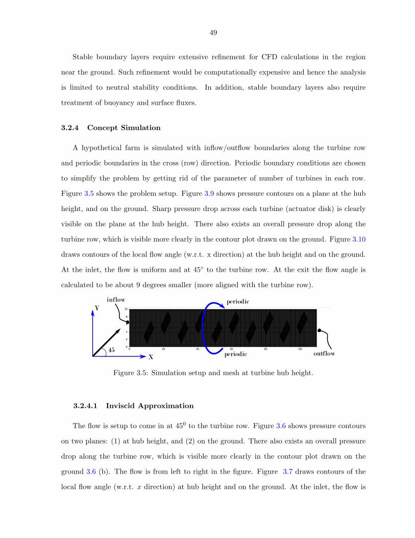
49
Stable boundary layers require extensive refinement for CFD calculations in the region
near the ground. Such refinement would be computationally expensive and hence the analysis
is limited to neutral stability conditions. In addition, stable boundary layers also require
treatment of buoyancy and surface fluxes.
3.2.4 Concept Simulation
A hypothetical farm is simulated with inflow/outflow boundaries along the turbine row
and periodic boundaries in the cross (row) direction. Periodic boundary conditions are chosen
to simplify the problem by getting rid of the parameter of number of turbines in each row.
Figure 3.5 shows the problem setup. Figure 3.9 shows pressure contours on a plane at the hub
height, and on the ground. Sharp pressure drop across each turbine (actuator disk) is clearly
visible on the plane at the hub height. There also exists an overall pressure drop along the
turbine row, which is visible more clearly in the contour plot drawn on the ground. Figure 3.10
draws contours of the local flow angle (w.r.t. x direction) at the hub height and on the ground.
At the inlet, the flow is uniform and at 45� to the turbine row. At the exit the flow angle is
calculated to be about 9 degrees smaller (more aligned with the turbine row).
Figure 3.5: Simulation setup and mesh at turbine hub height.
3.2.4.1 Inviscid Approximation
The flow is setup to come in at 450 to the turbine row. Figure 3.6 shows pressure contours
on two planes: (1) at hub height, and (2) on the ground. There also exists an overall pressure
drop along the turbine row, which is visible more clearly in the contour plot drawn on the
ground 3.6 (b). The flow is from left to right in the figure. Figure 3.7 draws contours of the
local flow angle (w.r.t. x direction) at hub height and on the ground. At the inlet, the flow is
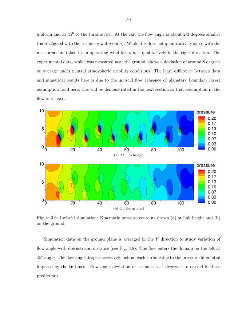
50
uniform and at 450 to the turbine row. At the exit the flow angle is about 2-3 degrees smaller
(more aligned with the turbine row direction). While this does not quantitatively agree with the
measurements taken in an operating wind farm, it is qualitatively in the right direction. The
experimental data, which was measured near the ground, shows a deviation of around 8 degrees
on average under neutral atmospheric stability conditions. The large di↵erence between data
and numerical results here is due to the inviscid flow (absence of planetary boundary layer)
assumption used here; this will be demonstrated in the next section as that assumption in the
flow is relaxed.
(a) At hub height
(b) On the ground
Figure 3.6: Inviscid simulation: Kinematic pressure contours drawn (a) at hub height and (b)on the ground.
Simulation data on the ground plane is averaged in the Y direction to study variation of
flow angle with downstream distance (see Fig. 3.8). The flow enters the domain on the left at
45o angle. The flow angle drops successively behind each turbine due to the pressure di↵erential
imposed by the turbines. Flow angle deviation of as much as 4 degrees is observed in these
predictions.
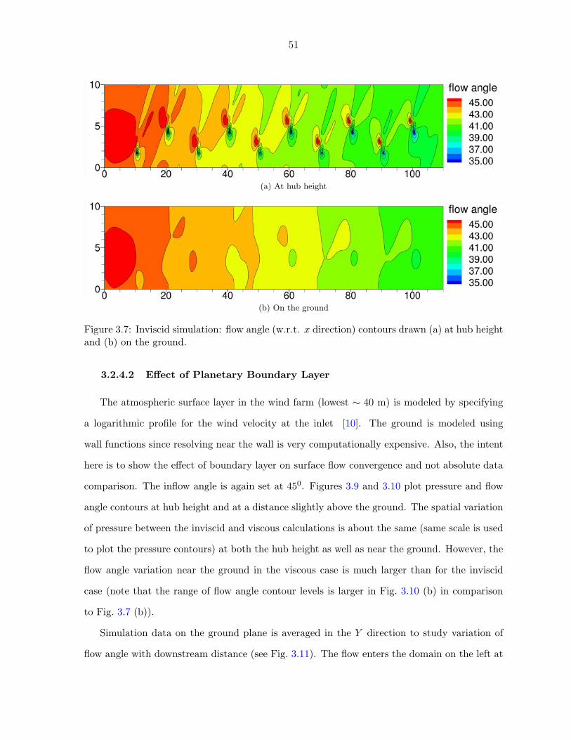
51
(a) At hub height
(b) On the ground
Figure 3.7: Inviscid simulation: flow angle (w.r.t. x direction) contours drawn (a) at hub heightand (b) on the ground.
3.2.4.2 E↵ect of Planetary Boundary Layer
The atmospheric surface layer in the wind farm (lowest ⇠ 40 m) is modeled by specifying
a logarithmic profile for the wind velocity at the inlet [10]. The ground is modeled using
wall functions since resolving near the wall is very computationally expensive. Also, the intent
here is to show the e↵ect of boundary layer on surface flow convergence and not absolute data
comparison. The inflow angle is again set at 450. Figures 3.9 and 3.10 plot pressure and flow
angle contours at hub height and at a distance slightly above the ground. The spatial variation
of pressure between the inviscid and viscous calculations is about the same (same scale is used
to plot the pressure contours) at both the hub height as well as near the ground. However, the
flow angle variation near the ground in the viscous case is much larger than for the inviscid
case (note that the range of flow angle contour levels is larger in Fig. 3.10 (b) in comparison
to Fig. 3.7 (b)).
Simulation data on the ground plane is averaged in the Y direction to study variation of
flow angle with downstream distance (see Fig. 3.11). The flow enters the domain on the left at
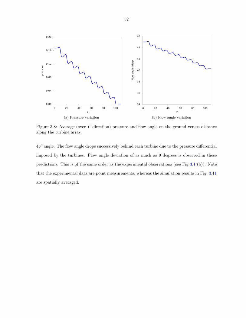
52
0.00
0.04
0.08
0.12
0.16
0.20
0 20 40 60 80 100
pre
ssure
X
(a) Pressure variation
34
36
38
40
42
44
46
0 20 40 60 80 100
Flow
angle
(deg)
X
(b) Flow angle variation
Figure 3.8: Average (over Y direction) pressure and flow angle on the ground versus distancealong the turbine array.
45o angle. The flow angle drops successively behind each turbine due to the pressure di↵erential
imposed by the turbines. Flow angle deviation of as much as 9 degrees is observed in these
predictions. This is of the same order as the experimental observations (see Fig 3.1 (b)). Note
that the experimental data are point measurements, whereas the simulation results in Fig. 3.11
are spatially averaged.
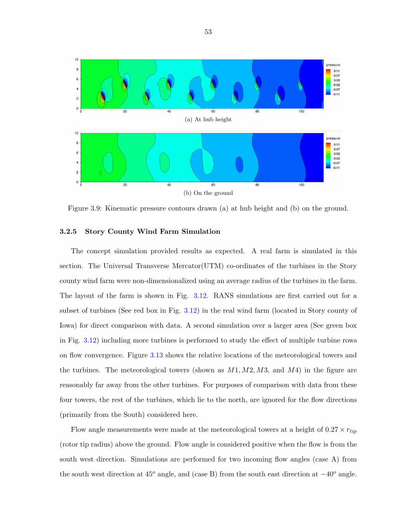
53
(a) At hub height
(b) On the ground
Figure 3.9: Kinematic pressure contours drawn (a) at hub height and (b) on the ground.
3.2.5 Story County Wind Farm Simulation
The concept simulation provided results as expected. A real farm is simulated in this
section. The Universal Transverse Mercator(UTM) co-ordinates of the turbines in the Story
county wind farm were non-dimensionalized using an average radius of the turbines in the farm.
The layout of the farm is shown in Fig. 3.12. RANS simulations are first carried out for a
subset of turbines (See red box in Fig. 3.12) in the real wind farm (located in Story county of
Iowa) for direct comparison with data. A second simulation over a larger area (See green box
in Fig. 3.12) including more turbines is performed to study the e↵ect of multiple turbine rows
on flow convergence. Figure 3.13 shows the relative locations of the meteorological towers and
the turbines. The meteorological towers (shown as M1, M2, M3, and M4) in the figure are
reasonably far away from the other turbines. For purposes of comparison with data from these
four towers, the rest of the turbines, which lie to the north, are ignored for the flow directions
(primarily from the South) considered here.
Flow angle measurements were made at the meteorological towers at a height of 0.27⇥ r
tip
(rotor tip radius) above the ground. Flow angle is considered positive when the flow is from the
south west direction. Simulations are performed for two incoming flow angles (case A) from
the south west direction at 45o angle, and (case B) from the south east direction at �40o angle.
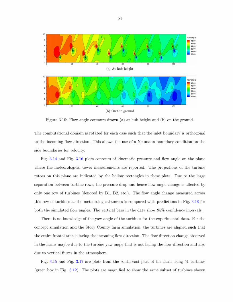
54
(a) At hub height
(b) On the ground
Figure 3.10: Flow angle contours drawn (a) at hub height and (b) on the ground.
The computational domain is rotated for each case such that the inlet boundary is orthogonal
to the incoming flow direction. This allows the use of a Neumann boundary condition on the
side boundaries for velocity.
Fig. 3.14 and Fig. 3.16 plots contours of kinematic pressure and flow angle on the plane
where the meteorological tower measurements are reported. The projections of the turbine
rotors on this plane are indicated by the hollow rectangles in these plots. Due to the large
separation between turbine rows, the pressure drop and hence flow angle change is a↵ected by
only one row of turbines (denoted by B1, B2, etc.). The flow angle change measured across
this row of turbines at the meteorological towers is compared with predictions in Fig. 3.18 for
both the simulated flow angles. The vertical bars in the data show 95% confidence intervals.
There is no knowledge of the yaw angle of the turbines for the experimental data. For the
concept simulation and the Story County farm simulation, the turbines are aligned such that
the entire frontal area is facing the incoming flow direction. The flow direction change observed
in the farms maybe due to the turbine yaw angle that is not facing the flow direction and also
due to vertical fluxes in the atmosphere.
Fig. 3.15 and Fig. 3.17 are plots from the south east part of the farm using 51 turbines
(green box in Fig. 3.12). The plots are magnified to show the same subset of turbines shown
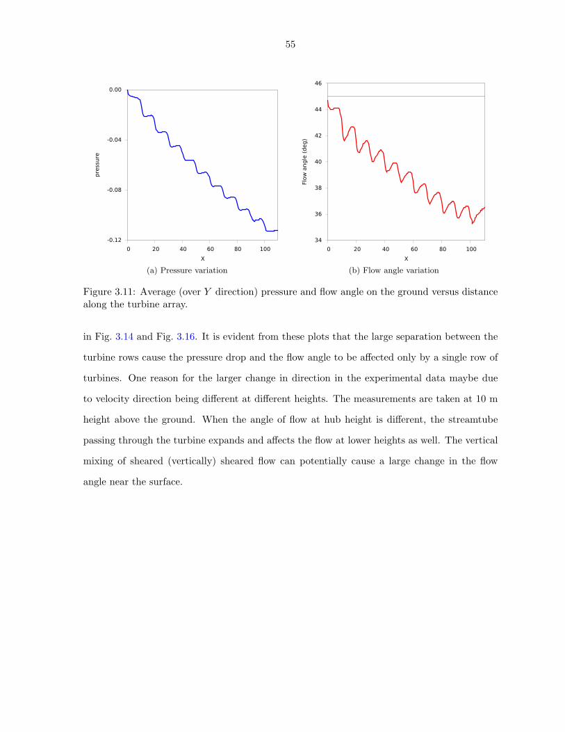
55
-0.12
-0.08
-0.04
0.00
0 20 40 60 80 100
pre
ssure
X
(a) Pressure variation
34
36
38
40
42
44
46
0 20 40 60 80 100
Flow
angle
(deg)
X
(b) Flow angle variation
Figure 3.11: Average (over Y direction) pressure and flow angle on the ground versus distancealong the turbine array.
in Fig. 3.14 and Fig. 3.16. It is evident from these plots that the large separation between the
turbine rows cause the pressure drop and the flow angle to be a↵ected only by a single row of
turbines. One reason for the larger change in direction in the experimental data maybe due
to velocity direction being di↵erent at di↵erent heights. The measurements are taken at 10 m
height above the ground. When the angle of flow at hub height is di↵erent, the streamtube
passing through the turbine expands and a↵ects the flow at lower heights as well. The vertical
mixing of sheared (vertically) sheared flow can potentially cause a large change in the flow
angle near the surface.
56
3.3 Conclusion
The numerical method developed in Ch. 1 is used to study a mesoscale meteorological phe-
nomenon called surface flow convergence. Flow coming at an angle to an array of wind turbines
has been observed to change its direction towards the turbine row direction near the ground.
A mesoscale, low-pressure inside the turbine array is believed to be the reason for this flow
convergence. To substantiate this hypothesis, a hypothetical wind farm, with periodic bound-
aries, is analyzed using the actuator disk model implementation in OpenFOAM. Simulations
are first conducted with inviscid flow approximation (uniform flow at the inlet). The pressure
drop inside the turbine array is observed however the magnitude of flow convergence is found to
be much smaller than measured. A viscous simulation with prescribed logarithmic atmospheric
surface layer at the inlet of the CFD domain is then conducted which exhibits similar pressure
drop as in the inviscid case; however, the flow turning near the ground is observed to be much
larger (of the order of measured values). The reduced dynamic pressure (because of reduced
velocity in the boundary layer) is responsible for the larger turning near the ground. A subset
of turbines from a real wind farm (Story County farm of Iowa) are simulated and compared to
experimental data. The e↵ect of neighboring rows on flow convergence was studied by analyz-
ing a larger area of the farm. Due to the large spacing between rows, the pressure recovers to
its freestream value and hence the change in flow direction is not predicted to be as large in
the case of a hypothetical wind farm.
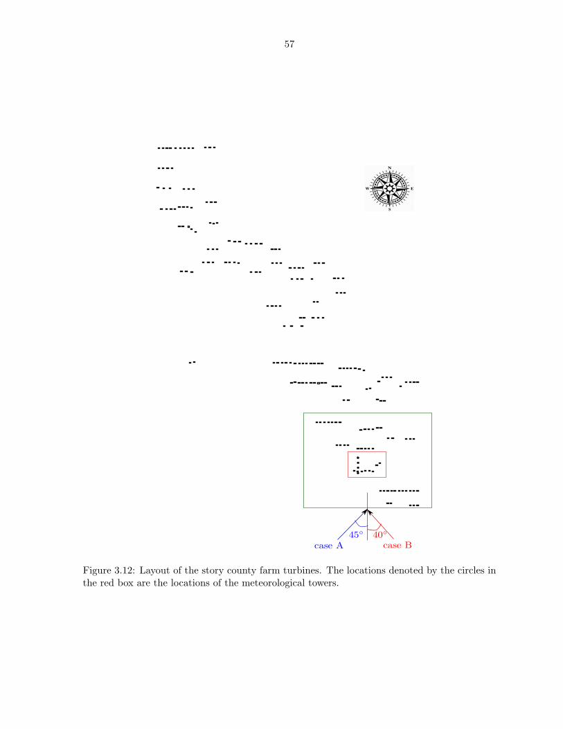
57
Figure 3.12: Layout of the story county farm turbines. The locations denoted by the circles inthe red box are the locations of the meteorological towers.
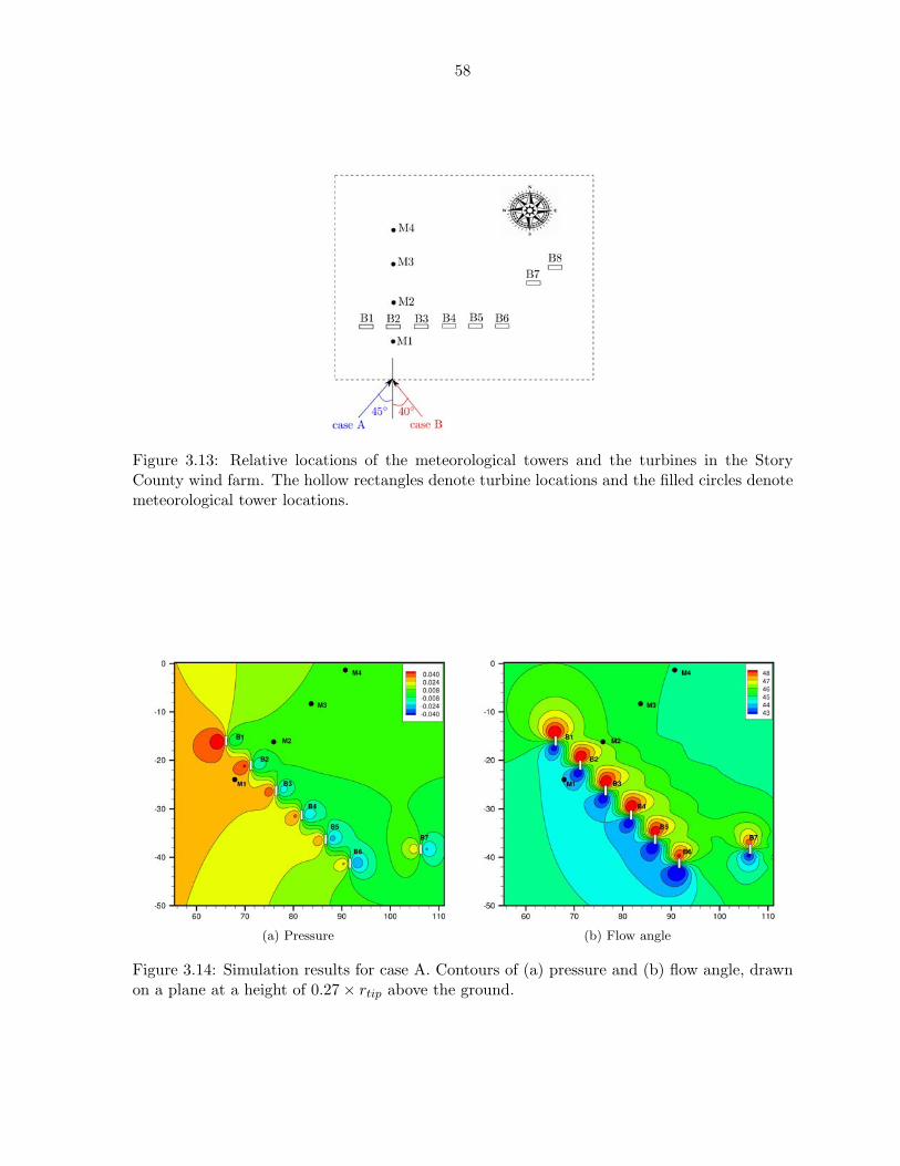
58
Figure 3.13: Relative locations of the meteorological towers and the turbines in the StoryCounty wind farm. The hollow rectangles denote turbine locations and the filled circles denotemeteorological tower locations.
(a) Pressure (b) Flow angle
Figure 3.14: Simulation results for case A. Contours of (a) pressure and (b) flow angle, drawnon a plane at a height of 0.27⇥ r
tip
above the ground.
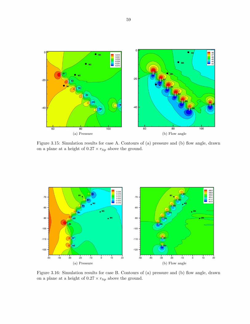
59
(a) Pressure (b) Flow angle
Figure 3.15: Simulation results for case A. Contours of (a) pressure and (b) flow angle, drawnon a plane at a height of 0.27⇥ r
tip
above the ground.
(a) Pressure (b) Flow angle
Figure 3.16: Simulation results for case B. Contours of (a) pressure and (b) flow angle, drawnon a plane at a height of 0.27⇥ r
tip
above the ground.
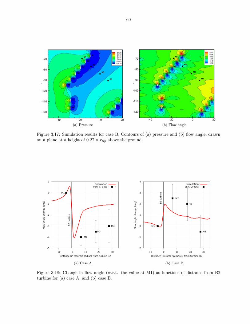
60
(a) Pressure (b) Flow angle
Figure 3.17: Simulation results for case B. Contours of (a) pressure and (b) flow angle, drawnon a plane at a height of 0.27⇥ r
tip
above the ground.
-5
-4
-3
-2
-1
0
1
-10 0 10 20 30
Flow
angle
change (
deg)
Distance (in rotor tip radius) from turbine B2
M1
M2
M3
M4B2
turb
ine
Simulation95% CI data
(a) Case A
-2
-1
0
1
2
3
4
-10 0 10 20 30
Flow
angle
change (
deg)
Distance (in rotor tip radius) from turbine B2
M1
M2
M3
M4
B2
turb
ine
Simulation95% CI data
(b) Case B
Figure 3.18: Change in flow angle (w.r.t. the value at M1) as functions of distance from B2turbine for (a) case A, and (b) case B.

61
Bibliography
[1] (2014). Stakeholder engagement and outreach: U.S. installed wind capacity. http://www.
windpoweringamerica.gov/wind_installed_capacity.asp.
[2] Ainslie, J. F. (1988). Calculating the flowfield in the wake of wind turbines. Journal of
Wind Engineering and Industrial Aerodynamics, 27(1):213–224.
[3] Ammara, I., Leclerc, C., and Masson, C. (2002). A viscous three-dimensional
di↵erential/actuator-disk method for the aerodynamic analysis of wind farms. Transactions-
American Society of Mechanical Engineers Journal of Solar Energy Engineering, 124(4):345–
356.
[4] Anderson Jr, J. D. (1985). Fundamentals of aerodynamics. Tata McGraw-Hill Education.
[5] Barthelmie, R. J. (2007). Modeling and measurements of wakes in large wind farms. Journal
of Physics: Conference Series, 75.
[6] Barthelmie, R. J. and Jensen, L. E. (2010). Evaluation of power losses due to wind turbine
wakes at the nysted o↵shore wind farm. Wind Energy, 13:573–586.
[7] Betz, A. (1919). Schraubenpropeller mit Geringstem Energieverlust. PhD thesis, Gottingen
Nachrichten.
[8] Churchfield, M., Lee, S., Michalakes, J., and Moriarty, P. (2012). A numerical study of the
e↵ects of atmospheric and wake turbulence on wind turbine dynamics. Journal of Turbulence,
13(14).
[9] Corten, G. P. and Lindenburg, P. S. (2007). Assembly of energy flow collectors, such as
windpark, and method of operation. US Patent 7299627 B2.
62
[10] D. M. Hargreaves and N. G. Wright (2007). On the use of the k-epsilon model in commercial
cfd software to model the neutral atmospheric boundary layer. Journal of Wind Engineering
and Industrial Aerodynamics, 95:355–369.
[11] Energy Information Administration, U. (2014). Electric power monthly. U.S. Department
of Energy.
[12] Frandsen, S., Barthelmie, R., Pryor, S., Rathmann, O., Larsen, S., Højstrup, J., and
Thøgersen, M. (2006). Analytical modelling of wind speed deficit in large o↵shore wind
farms. Wind Energy, 9(1-2):39–53.
[13] Goldstein, S. (1929). On the Vortex Theory of Screw Propellers. Proceedings of the Royal
Society A: Mathematical, Physical and Engineering Sciences, 123(792):440–465.
[14] Hansen, K. S., Barthelmie, R. J., Jensen, L. E., and Sommer, A. (2012). The impact of
turbulence intensity and atmospheric stability on power deficits due to wind turbine wakes
at horns rev wind farm. Wind Energy, 15(1):183–196.
[15] Hargreaves, S. (2012). What we got for 50 billion in green stimulus. http://money.cnn.
com/2012/10/03/news/economy/green-stimulus/. Accessed February 7, 2014.
[16] I. H. Abbott and A. E. von Doenho↵ (1959). Theory of Wing Sections Including a Summary
of Airfoil Data. Dover Publications, Inc.
[17] J. G. Schepers, A. J. Brand, A. Bruining, J. M. R. Graham, M. M. Hand, D. G. Infield, H.
A. Madsen, R. J. H. Paynter, and D. A. Simms (1997). Final report of iea annes xiv: Field
rotor aerodynamics. ECN-C–97-027.
[18] Jenkins, M. (2005). Unit 7: Atmospheric stability and instability. http:
//ocw.usu.edu/Forest__Range__and_Wildlife_Sciences/Wildland_Fire_Management_
and_Planning/Unit_7__Atmospheric_Stability_and_Instability_1.html. Accessed
April 4, 2014.
63
[19] Johnson, K. E. and Thomas, N. (2009). Wind farm control: Addressing the aerodynamic
interaction among wind turbines. In American Control Conference, 2009. ACC’09., pages
2104–2109. IEEE.
[20] Jonkman, J., Butterfield, S., Musial, W., and Scott, G. (2009). Definition of a 5-mw
reference wind turbine for o↵shore system development. In NREL/TP-500-38060, Colorado.
National Renewable Energy Laboratory.
[21] Jung, S. N., No, T.-S., and Ryu, K.-W. (2005). Aerodynamic performance prediction of a
30kw counter-rotating wind turbine system. Renewable Energy, 30(5):631–644.
[22] Kanemoto, T. and Galal, A. M. (2006). Development of intelligent wind turbine generator
with tandem wind rotors and double rotational armatures (1st report, superior operation of
tandem wind rotors). JSME International Journal Series B, 49(2):450–457.
[23] Katic, I., Højstrup, J., and Jensen, N. (1986). A simple model for cluster e�ciency.
[24] Kumar, P. S., Abraham, A., Bensingh, R. J., and Ilangovan, S. (2013). Computational
and experimental analysis of a counter-rotating wind turbine system. Journal of Scientific
& Industrial Research, 72(5):300–306.
[25] Larsen, G. C., Højstrup, J., and Aagaard Madsen, H. (1996). Wind fields in wakes.
[26] Lee, S., Kim, H., and Lee, S. (2010). Analysis of aerodynamic characteristics on a counter-
rotating wind turbine. Current Applied Physics, 10(2):S339–S342.
[27] Lee, S., Kim, H., Son, E., and Lee, S. (2012). E↵ects of design parameters on aerodynamic
performance of a counter-rotating wind turbine. Renewable Energy, 42:140–144.
[28] Mackay, D. (2008). Sustainable Energy without the hot air. UIT Cambridge Ltd.
[29] Mandas, N., Cambuli, F., and Carcangiu, C. E. (2006). Numerical prediction of horizontal
axis wind turbine flow. University of Cagliari, Department of Mechanical Engineering.
[30] Mikkelsen, R. (2003). Actuator Disk Models Applied to Wind Turbines. PhD thesis,
Technical University of Denmark.
64
[31] M.M. Hand, D.A. Simms, L.J. Fingersh, D.W. Jager, J.R. Cotrell, S. Schreck, and S.M.
Larwood (2001). Unsteady Aerodynamics Experiment Phase VI: Wind Tunnel Test Config-
urations and Available Data Campaigns. NREL Technical Report, NREL/TP-500-29955.
[32] Newman, B. (1986). Multiple actuator-disc theory for wind turbines. Journal of Wind
Engineering and Industrial Aerodynamics, 24(3):215–225.
[33] Okulov, V. L. (2004). On the stability of multiple helical vortices. Journal of Fluid
Mechanics, 521:319–342.
[34] Okulov, V. L. and Sø rensen, J. N. (2008a). An ideal wind turbine with a finite number
of blades. Doklady Physics, 53(6):337–342.
[35] Okulov, V. L. and Sø rensen, J. N. (2008b). Refined Betz limit for rotors with a finite
number of blades. Wind Energy, 11(4):415–426.
[36] Porte-Agel, F., Wu, Y., Lu, H., and Conzemius, R. J. (2011). Large-eddy simulation of
atmospheric boundary layer flow through wind turbines and wind farms. Journal of Wind
Engineering and Industrial Aerodynamics, 99:154–168.
[37] Rosenberg, A., Selvaraj, S., and Sharma, A. (2014). A novel dual-rotor turbine for in-
creased wind energy capture. In Proceedings of the Conference on The Science of Making
Torque from Wind. Torque, Technical University of Denmark.
[38] S. Lissaman, P. (1979). Energy e↵ectiveness of arbitrary arrays of wind turbines. Journal
of Energy, 3(6):323–328.
[39] Sanderse, B., Pijl, S. P. v. d., and Koren, B. (2011). Review of computational fluids
dynamics for wind turbine wake aerodynamics. Wind Energy.
[40] Selig, M. (2012). Propid user manual.
[41] Selig, M. and Tangler, J. L. (1995). Development and application of a multipoint inverse
design method for horizontal axis wind turbines. Wind Engineering, 19(2).
65
[42] Selvaraj, S., Chaves, A., Takle, E., and Sharma, A. (2013). Numerical prediction of
surface flow convergence phenomenon in windfarms. In Proceedings of the Conference on
Wind Energy Science and Technology, METU, Ankara, Turkey. RUZGEM, Middle Eastern
Technical University.
[43] Sharma, A., Taghaddosi, F., and Gupta, A. (2010). Diagnosis of aerodynamic losses in
the root region of a horizontal axis wind turbine. Niskayuna, New York. General Electric
Internal Report.
[44] Sørensen, J. N. and Shen, W. Z. (2002). Numerical modeling of wind turbine wakes.
Journal of Fluids Engineering, 124(2):393–399.
[45] Takle, E. S. (2012). Private communication.
[46] Tangler, J. L. and Somers, D. M. (1995). NREL airfoil families for HAWTs. National
Renewable Energy Laboratory.
[47] Ushiyama, I., Shimota, T., and Miura, Y. (1996). An experimental study of the two-staged
wind turbines. Renewable energy, 9(1):909–912.
[48] Vermeer, L., Sørensen, J. N., and Crespo, A. (2003). Wind turbine wake aerodynamics.
Progress in aerospace sciences, 39(6):467–510.
[49] Wilson, R. E., Lissaman, P. B. S., and Walker, S. N. (1976). Aerodynamic performance
of wind turbines. NASA STI/Recon Technical Report N, 77:18598–+.
[50] Wobben, A. (2006). Wind power installation with two rotors in tandem. US Patent
7,074,011 B1.
[51] Yuan, W., Ozbay, A., Tian, W., and Hu, H. (2013). An experimental investigation on
the e↵ects of turbine rotation directions on the wake interference of wind turbines. AAIA
Aerospace sciences meeting.