Numerical investigation on the cavitation collapse regime around the submerged vehicles navigating with deceleration

European Journal of Mechanics B/Fluids 49 (2015) 153–170

Contents lists available at ScienceDirect

European Journal of Mechanics B/Fluids

journal homepage: www.elsevier.com/locate/ejmflu

Numerical investigation on the cavitation collapse regime around thesubmerged vehicles navigating with deceleration

Ying Chen a,b,∗, Chuanjing Lu a,b,c, Xin Chen a,b, Jiayi Cao a,b

a School of Naval Architecture, Ocean and Civil Engineering, Shanghai Jiao Tong University, Shanghai 200240, Chinab MOE Key Laboratory of Hydrodynamics, Shanghai Jiao Tong University, Shanghai 200240, Chinac State Key Laboratory of Ocean Engineering, Shanghai Jiao Tong University, Shanghai 200240, China

a r t i c l e i n f o

Article history:Received 7 February 2014Received in revised form18 August 2014Accepted 19 August 2014Available online 28 August 2014

Keywords:Cavitating flowNumerical simulationCollapseSubmergedDeceleration

a b s t r a c t

In the presentwork, the collapse regimes of the cavitation occurring on the submerged vehicles navigatingwith deceleration were numerically investigated. A homogeneous equilibrium cavitation model wascombined with the pressure–velocity–density coupling algorithm to simulate the cavitating flows. Thecavity is induced to collapse by the deceleration after fluctuation, and the first collapse releasing most ofthe energy is followed by a series of secondary ones. The collapse process can be classified into two types:periodic oscillation and damped oscillation. In each type the evolution of the total mass of vapor in cavityis found to have strict correlation with the pressure oscillation in the far field. The two types are differentin the intensity and the bandwidth of the pressure peaks. By defining the equivalent radius of cavity, weintroduce the specific kinetic energy of collapse anddemonstrate that its change-rate is in good agreementwith the pressure disturbance. It is also found that the drag presents corresponding oscillations. Throughcomparative analysis on the velocity field and the stress distribution along the body, it indicates that thecollapse can produce extremely high pressure instantaneously.Wenumerically investigated the influenceof the angle of attack on the collapse regime. The result shows that when the vehicle decelerates, anasymmetric-focusing effect of the pressure induced by collapse occurs on its pressure side.We analyticallyproved such an asymmetric-focusing effect using the potential flow theory. The mathematical model andmethod we proposed show capability in reflecting the evolution of the pressure difference between bothsides of the vehicle.

© 2014 Elsevier Masson SAS. All rights reserved.

1. Introduction

As a fundamental property of liquid, cavitation appears whenthe local static pressure in liquid falls below the saturated vaporpressure. It usually occurs in the flows of many hydraulic devices,such as turbines, pumps, pipe systems, fuel injectors, etc. On theother hand, partial sheet/cloud cavitation also often occurs aroundthe high-speed underwater vehicles moving upwards or cruisingnear the sea surface. In practical use, the deceleration of thevehicles caused by flow resistance or propulsion reasonmay resultin the unstable evolution of the cavity, which will significantlyaffect the hydrodynamic loads acting on the vehicle’s body.

∗ Corresponding author at: School of Naval Architecture, Ocean and CivilEngineering, Shanghai Jiao Tong University, Shanghai 200240, China. Tel.: +8613761302148; fax: +86 2134204308.

E-mail address: [email protected] (Y. Chen).

http://dx.doi.org/10.1016/j.euromechflu.2014.08.0050997-7546/© 2014 Elsevier Masson SAS. All rights reserved.

The experimental researches on cavitation have been exten-sively carried out so far for varieties of flows, most of whichare around hydrofoils or propellers. However the available re-search record about the cavitation around submerged axisym-metric bodies in the literature is quite few due to its militaryapplication background. In the middle of the last century, Rouseand McNown [1] carried out a series of experiments on the cavi-tating flows about axisymmetric configurationswith cylindrical af-terbody. In this century, Savchenko [2] performed an experimentalstudy on the high-speed supercavitating flows around underwa-ter projectile. Vlasenko [3] investigated the hydrodynamic forceson the cavitated axisymmetric bodies moving in water. Huanget al. [4] used a high-speed camera and a force measurement sys-tem to study the unsteady cavitating flow patterns and resistanceof the 0-caliber ogive revolution bodies under different conditions.

In the CFD framework for cavitation simulation, different kindsof two-phase flow approaches have been developed. In the pasttwo decades, the one-fluid model has been widely used, in which

http://dx.doi.org/10.1016/j.euromechflu.2014.08.005

http://www.elsevier.com/locate/ejmflu

http://www.elsevier.com/locate/ejmflu

http://crossmark.crossref.org/dialog/?doi=10.1016/j.euromechflu.2014.08.005&domain=pdf

mailto:[email protected]

http://dx.doi.org/10.1016/j.euromechflu.2014.08.005

154 Y. Chen et al. / European Journal of Mechanics B/Fluids 49 (2015) 153–170

the cavitating flow field is treated as filled with a homogeneousmixture composed of the liquid and vapor phases, and the flow isgoverned by only one set of equations.

Kubota et al. [5] proposed the bubble two-phase flow (BTF)model using the Rayleigh–Plesset equation. Schnerr and Sauer [6]and Frobenius et al. [7] further improved it. Themodelswere foundto be suitable for the cloud cavitation with relatively low purenessof vapor. Another way of the one-fluid model is the barotropicequationmodel proposed by Delannoy and Kueny [8], in which thedensity of mixture is directly linked with the local pressure andthe phase-change process is neglected. Although the numericalstability during computation is hard to be guaranteed, this type ofmodel has been successfully used to simulate unsteady cavitatingflows by Coutier-Delgosha et al. [9] and Byeong et al. [10].Goncalves [11] as well presented such a model using two differentliquid–vapormixture EOS and a preconditioning scheme to handleany Mach number.

The third and also currently the most popular way is wellknown as the transport equation model (TEM), in which an equa-tion for the liquid or vapor phase fraction is solved. Merkleet al. [12], Kunz et al. [13], Yuan et al. [14] and Singhal et al. [15] re-spectively proposed suchmodels where the phase-change sourcesare related to the amount by which the local pressure is below thesaturated vapor pressure. Kunz et al. [13] predicted the steady stateand transient cavitation on a series of ogive forebody cylinderswith an angle of attack. Lindau et al. [16] andKimet al. [17] also uti-lized the Kunz model to investigate the unstable 3-D effect of thecavitating flows over axisymmetric bodies with blunt and hemi-spheric noses. Owis and Nayfeh [18] adopted the Merkle modelto simulate the cavitating flows over projectiles with differentgeometries using a preconditioning dual-time stepping method.Senocak and Shyy [19] evaluated the capability of the above men-tioned versions of TEM on the prediction of steady cavity on ax-isymmetric bodies. Goncalves [20] also investigated the behaviorof various TEMs and compared a range ofmodels from three to fiveequations. Recently, Goncalves and Charriere [21] proposed a va-por ratio TEMusing an original source term formass transferwhichwas assumed to be proportional to the divergence of the homoge-neous velocity field. In thismodel a particular emphasiswas placedon the thermodynamic coherence.

Some other important approaches in cavitation modeling havealso been developed, especially the ones considering the thermo-dynamic effect. Barberon and Helluy [22] proposed a projection fi-nite volume scheme to resolve the difficulties in the pressure lawtaking into account phase transitions, such as the non-uniquenessof the entropy solution. Gavrilyuk and Saurel [23] developed amodel with full coupling between micro- and macroscale motionfor compressiblemultiphasemixture, and themodelwas validatedfor the interaction of wave with bubbles. Saurel et al. [24] con-structed a hyperbolic two-phase flow model involving five par-tial differential equations for phase interface modeling. The modelis able to deal with phase transition fronts where heat and masstransfer occur. In recent years, Petitpas et al. [25,26] used Saurel’smodel to compute the compressible cavitating flows around high-speed underwater missiles.

The unstable behavior of sheet/cloud cavitation has beenwidely investigated on hydrofoils, and its instability has beenconsidered to be primarily caused by the re-entrant jet. However,the minor studying of the cavitation around axisymmetric bodiesas mentioned above has mainly been focused on its evolution innormal conditions. The collapse of cavitation in the deceleratingnavigation state has seldom been discussed so far. The primaryobjective of this work is to numerically investigate the collapsebehavior of the partial cavitation around decelerating 3-D vehiclesand its influence on the hydrodynamic forces.

2. Mathematical model and numerical methods

The present numerical works were carried out using the com-mercial CFD solver ANSYS FLUENT 14.0. The mathematical modeland numerical methods we adopted will be briefly introducedhere.

2.1. Governing equations

The thermal effect of cavitating flows is often negligible in nor-mal situations, except for the liquids of extremely low temperatureor in the tiny region where the final stage of collapse occurs [27].Thus cavitating flowsusually can be regarded as isothermal inmostpart or stage of the cavitation evolution, allowing one to avoid solv-ing the energy equation. The governing equations include the con-tinuity equation and the compressible RANS equation:

∂ρm

∂t+

∂ρmuj

∂xj

= 0 (1)

∂ (ρmui)

∂t+

∂ρmujui

∂xj

=∂

∂xj

(µm + µt)

∂ui

∂xj+

∂uj

∂xi

−

∂

∂xi

p +

23µm

∂uk

∂xk

(2)

where ρm denotes the density of the mixture, and µm and µt de-note the molecular viscosity and turbulent viscosity respectively.These material properties need to be determined by the cavitationmodel described in the following subsection.

Majority of the cavitation simulations in the literature haveused conventional eddy-viscosity turbulence models. In thepresent work, the turbulence effect is modeled using the RNG k–εmodel which will be validated in Section 4.3. The model equationsare as follows:

∂ (ρmk)∂t

+∂ρmujk

∂xj

=∂

∂xj

αk (µm + µt)

∂k∂xj

+ 2µtSijSji − Ckρmε (3)

∂ (ρmε)

∂t+

∂ρmujε

∂xj

=∂

∂xj

αε (µm + µt)

∂ε

∂xj

+ Cε1

ε

k

2µtSijSji − C∗

ε2ρm

ε2

k

(4)

where the generation sources due to buoyancy and fluctuatingdilatation are not taken into account, αk and αε are the inverseeffective Prandtl numbers analytically derived by the RNG theory,and the model parameters are specified as: Ck = 1.0, Cε1 = 1.42.The C∗

ε2 is defined as:

C∗

ε2 = Cε2 +Cµη3(1 − η/η0)

1 + βη3(5)

where Cε2 = 1.68, Cµ = 0.0845, β = 0.012, η0 = 4.38, andη =

2SijSjik/ε.

2.2. Cavitation model

Due to the variable density of themixture in the flow, additionalequations for density are necessary for the equations system tobe closed. An optional cavitation model in FLUENT suggested byZwart et al. [28] is used in this study. In previous works (see[29,30]) this model has been compared with other widespreadmodels in the literature (see [13,15]) for the prediction of thepressure distribution inside the cavitation region, and it was foundthat the different models can offer the same level of accuracy.

Y. Chen et al. / European Journal of Mechanics B/Fluids 49 (2015) 153–170 155

The density ρm is a function of vapor volume fraction αv whichis computed by solving a transport equation coupled with theconservation equations:ρm = αvρv + (1 − αv)ρl (6)µm = αvµv + (1 − αv)µl (7)

∂ (ρvαv)

∂t+

∂

∂xj

ρvujαv

= Se + Sc (8)

dρm

dt= −(ρl − ρv)

dαv

dt(9)

where ρv and ρl denote the density of the pure vapor and liquidphases in working condition. The source terms Se and Sc accountfor themass transfer between the phases. They should naturally berelated to the local pressure representing the change of themixturewhich takes the form of small bubble cluster.

Pure liquid even can withstand negative absolute pressurewithout phase change. The cavitation behavior of liquid stronglydepends on its air content [27]. In most engineering simulations,the mixture is assumed to be composed of plenty of bubbleswith the same size at any instant, because so far there is noreliable physical model, even the thermodynamic model, for theconsideration of bubble size distribution.

The single bubble dynamics can be modeled through thesimplified Rayleigh–Plesset equation, neglecting the second orderterm and the surface tension, as shown below:

dRdt

=

23pv − p

ρl. (10)

The vapor volume fraction is related to the bubble numberdensity n and the bubble radius R in the cavitation structure. Thisapproach has been successfully used inmany other popularmodels(see e.g. [14,15]).

αv = n43πR3. (11)

If the interaction between bubbles is neglected, and the masstransfer between liquid and vapor phases is assumed to be nearlyisothermal, the interphase mass transfer rate S was proposed(see [28]) to be calculated by combining the above mentionedequations:

S =3αvρv

R

23pv − p

ρl. (12)

The mass transfer rate is derived assuming bubble growth(evaporation). To apply it to the bubble collapse process (conden-sation) aswell, the final form of this cavitationmodel is formulatedas follows:

Se = Ce3α0(1 − αv)ρv

RB

23max

pv − p

ρl, 0

(13)

Sc = Cc3αvρv

RB

23max

p − pv

ρl, 0

(14)

where Ce and Cc are the empirical constants chosen to be 50 and0.01 respectively, α0 denotes the initial void fraction in water dueto the dissolved gas nucleus, RB denotes the initial nucleus radius,and the subscripts l and v denote the liquid and vapor phases,respectively.

The model is derived from the empirical bubble cluster dynam-ics and can inherently describe the unstable features of the macro-scopic bubble cluster, which reflects the averaged behavior ofnumerous microscopic bubbles. Therefore, the evolution of thecavitation simulated using this model can be compatible and co-herent with the analysis of the cavitation package collapse in anapproximate bubble dynamics way, as shown in Section 5.1.

2.3. Numerical strategy

The FLUENT solver employs the node-centered finite volumemethod. The numerical strategy is grounded on the pressure-basedsegregated RANS solver, accelerated by an algebraic multigrid(AMG) method, to solve the governing equations with a fullyimplicit discretization at any given time step. The SIMPLE-typepressure–velocity–density coupling correction method for thearbitrary Mach number [31] is employed, where the correctionequation of pressure contains convective and unsteady terms, i.e.is a convected wave equation.

Experiments and mathematical deductions [32–34] both indi-cate that in cavitating flows the speed of sound in the liquid/vapormixture is reduced to around ten meters per second, much lowerthan that of the single phases. Thus the local Mach number in theentire field will distribute in a wide range.

At a low Mach number, the Laplacian term in the correctionequation dominates and it recovers to the Poisson equation. At ahigh Mach number, the convective term dominates, reflecting thehyperbolic nature of the flow. Thus the coupling correctionmethodautomatically adjusts to the local nature of the flow and the samemethod can be applied to the entire flow.

A second order implicit transient formulation is used in per-forming the time-dependent computation, to acquire a relativelyaccurate capture for the cavitation collapse. The second order up-wind scheme is used to calculate the convection in themomentumand turbulence equations. TheQUICKdiscretization scheme is usedwhen solving the volume fraction equation of the cavitationmodel.The numerical result of third order accuracy will automatically beachieved after the iteration has converged. A least squares cell-based evaluation method using the Gram–Schmidt process [35] isused to compute the gradients of the variables appearing in thegoverning equations.

3. Problem description

In the present work, the unsteady cavitating flows around sev-eral submerged vehicles navigating with continuous decelerationare investigated. Three cylindrical vehicleswith blunt, hemisphericand conic noses are considered here. The shape of the vehicles andthe computational conditions are presented.

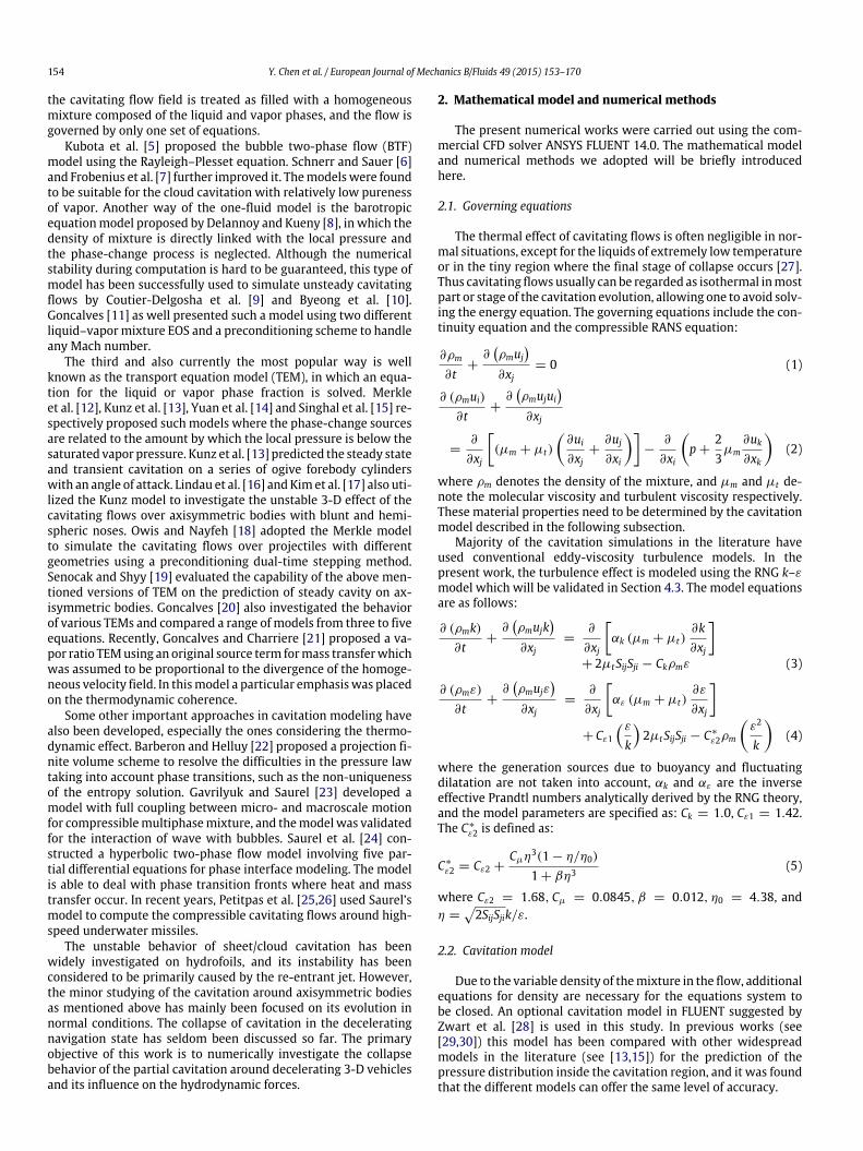
In Fig. 1, the 3-D vehicles and the configuration of the computa-tional domains are illustrated in the view of axisymmetric section.The computationalmeshes near the vehicle nose are shownaswell.The radius of the cylindrical part of the vehicles, Rn, is equal to 1m,and the length of the vehicles is 10 m. The working medium is wa-ter whose saturated vapor pressure is specified as pv = 3540 Pa.

The density of the liquid phase is specified as ρl = 1000 kg/m3

because of the low subsonic navigation speed. As for the densityof the vapor phase, constant value and ideal gas law both havebeen widely adopted by the researchers (see [12–19]). Neitherof them could be said to be a more ‘‘physical’’ one, because thefluid is artificially regarded as a hybrid of the pure phases whichare not inherent. Actually, there is little influence on the mixturedensity no matter which way is used, because the vapor fractionαv rapidly tends to zero in the region where the local pressureis higher than the vapor pressure pv , and the pressure inside thecavity is close to pv all the while. Therefore we specify the vapordensity as the constant value at a standard ambient condition, i.e.ρv = 0.5542 kg/m3.

The vehiclesmove leftwards in an infinite stationarywater area.The freestream velocity, V∞, at the boundaries of the computa-tional domain is set to be zero. A constant pressure is specified atthe downstream boundary to adjust the initial cavitation numberσ . The motion of the vehicles is achieved by dynamic mesh that


a

b

c

Fig. 1. Sketch of the computational models and domains.

can be used to specify the time variation of the motion speed ofthe vehicle and the whole computational domain.

In the practical case of the vehicle cruising beneath the seasurface, it may move in a completely free motion if the transientpropulsion problemoccurs. In the strict sense, one should calculatethe motion of the vehicle coupled with the computation of theflow field. However, in this way it might be difficult to decoupleand separately analyze the influence of the motion on cavity’sevolution and the influence of the cavity’s collapse on vehicle’smotion. It can be beneficial for investigating the collapse effect ifwe specify a forced motion of the vehicle.

The initial navigation velocity Ub0 is specified as 30 m/s. Itis achieved by speeding up from zero velocity to Ub0 in a timeduration of 0.2 s, and then keeping this velocity in a subsequenttime duration to the instant of t = t0, which can be flexiblyspecified according to the specific cavitation number. Then thevehicle is continuously decelerated to an ultimate velocityUbt fromthe instant of t = t0 to t = t1. In the present work, Ubt is specifiedas 20 m/s and t1 − t0 is 0.2 s. Computational cases at a series ofcavitation number have been performed.

The velocity variation is described by the piecewise functionshown in Eq. (15). It indicates that a constant minus accelerationis imposed when n is equal to 1, and stronger nonlinear minusacceleration is imposed when n is greater.

Ub =

Ub0

0.2t t < 0.2

Ub0 0.2 < t < t0

Ubt +

t0 − t0.2

+ 1n

(Ub0 − Ubt) t0 < t < t1

Ubt t1 < t.

(15)

4. Verification and validation

4.1. Mesh convergence analysis

In numerical simulations, the quality of computational meshusually has a significant influence on the accuracy of numericalresults. The mesh should have adequate fineness to ensure that

Table 1Mesh parameters.

Mesh series Radial grid size at themaximal cavity interface

Axial and radialnode amounts

Coarsest 0.294Rn 150 × 50Coarse 0.119Rn 300 × 100Medium 0.073Rn 450 × 150Fine 0.053Rn 600 × 200

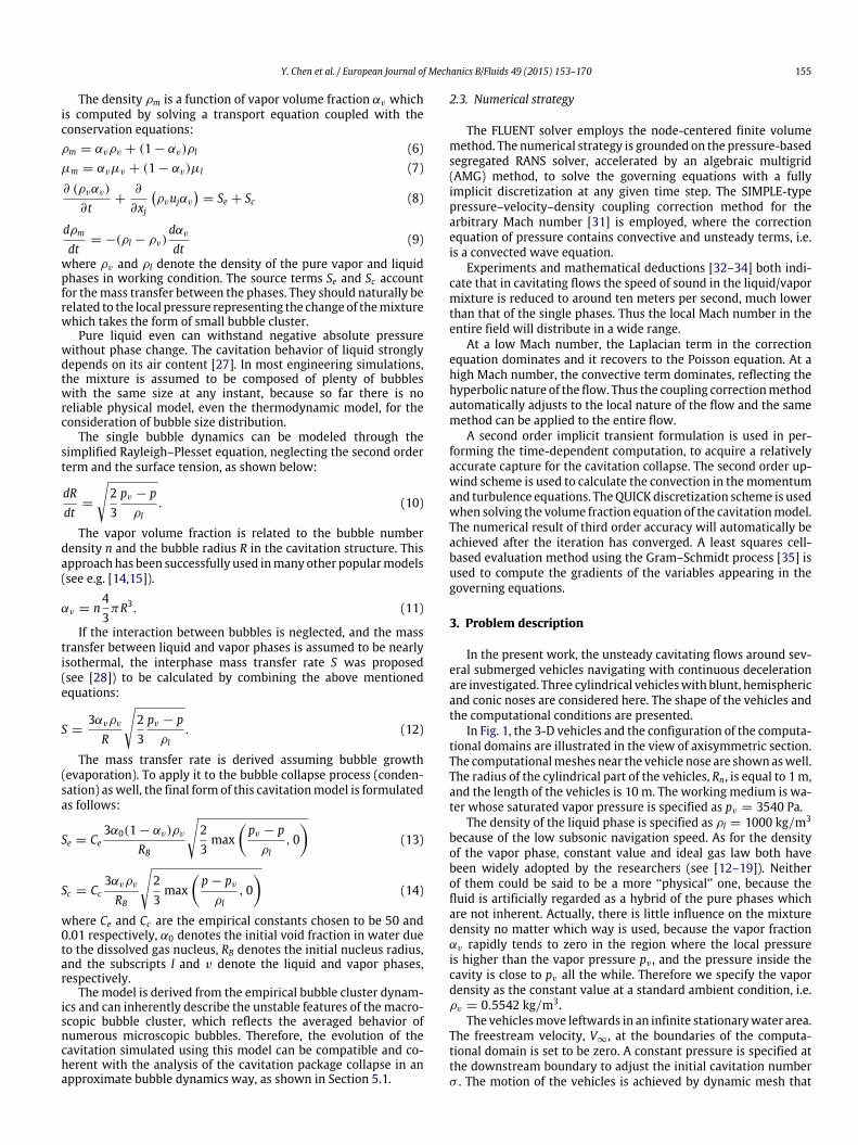
Fig. 2. Filled contours of the vapor fraction computed with different meshes:(a) coarsest mesh; (b) coarse mesh; (c) medium mesh; (d) fine mesh.

the results obtained are worth to be compared with experimentalresults and discussed further.

In this section, the mesh convergence is analyzed based on thecomputation cases about the blunt-nose vehicle. The computationswere performed at the cavitation number of σ = 0.3 on four setsof meshes with different fineness, as shown in Table 1. The totalcomputation time in each case is one second.

A comparatively stable cavity shape has been obtained oneach mesh before the deceleration occurs. The cavity shapes arecompared in Fig. 2. It can be observed that the cavity interface is abit thick and obscurewhen the coarsestmesh is used, but it rapidlybecomes much clearer after the mesh is refined to the ‘‘coarse’’one. The cavity shape hardly changes when the ‘‘medium’’ meshor ‘‘fine’’ mesh is used.

Table 2 gives the comparison between the maximal cavitylength and cavity thickness defined using the contour line of αv =

0.1, and the cavity interface thickness defined using the radialdistance between the contour lines ofαv = 0.1 andαv = 0.9 at theaxial position of maximal cavity thickness. The cavity lengths havelittle difference on all the meshes, and the relative error betweenthe last two meshes is below 0.05%. The relative error betweenthe cavity thicknesses computed on each two neighboring meshesdrops from 9.1% to 0.3%. The relative error of the cavity interfacethickness decreases from 44% to 5.4%.

Fig. 3 presents the comparison of the predicted pressurecoefficient distribution along the vehicle’s surface. Where the s inabscissa denotes the length of the curve along the wall from thetip of the nose, and D denotes the diameter of the vehicle. Fig. 4shows the comparison of the time histories of the drag coefficient.The drag coefficient is calculated based on the initial navigationspeed, Ub0 = 30 m/s, other than the instantaneous speed. The


Table 2Cavity sizes computed with the different meshes.

Mesh Cavitylength (m)

Cavitythickness (m)

Cavity interfacethickness (m)

Coarsest 8.603 1.335 0.593Coarse 8.624 1.213 0.333Medium 8.635 1.163 0.259Fine 8.640 1.159 0.245

Fig. 3. Comparison of the pressure coefficient distributions along the vehicle’ssurface computed with the different meshes (σ = 0.3).

Fig. 4. Comparison of the drag coefficients predicted with the different meshes(σ = 0.3).

curves change obviously when the ‘‘coarsest’’ mesh is refined, butare close to each other for the ‘‘medium’’ and the ‘‘fine’’ ones.

Although it indicates that the accuracy of the ‘‘medium’’ meshis sufficient, we still use the ‘‘fine’’ one in the following simulationsto guarantee the numerical precision, because the extra computa-tional cost is affordable to us.

4.2. Time step validation

To justify whether the time step used to capture the evolutionof the cavity is coherent with the Rayleigh formulation of the masssource term in the cavitation model describing the bubble clusterdynamics, the influence of time step on the computational results

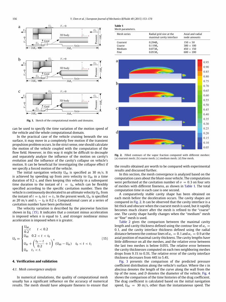
Fig. 5. Time histories of the total mass of vapor inside the flow fields calculatedwith different time steps (blunt-nose, σ0 = 0.3).

must be considered first. Several time steps have been examinedbythe computation of the flows after deceleration begins with n = 3at the initial cavitation number σ0 = 0.3.

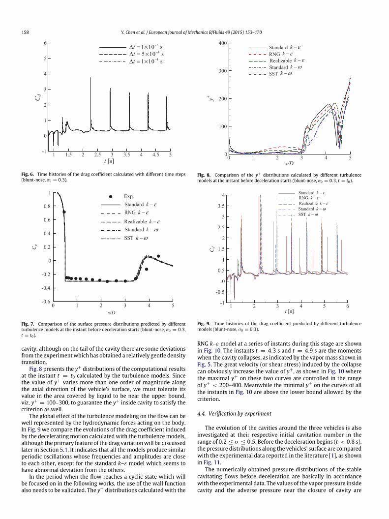
In Fig. 5 we compare the time histories of the total vapor massin the flow fields around the blunt-nose vehicle calculated usingdifferent time steps. The variation of the vapor mass representsthe collapse and regrowth of the cavity, which will be discussed indetail later in Section 5.1. It indicates that the size of time step doesnot affect the frequency and the intensity of the collapse, but has alittle influence on the cavity size which is reflected from the crestof the curve. When the time step is refined to 1t = 1 × 10−4 s,the maximal cavity size tends to converge after a periodic stateis attained. Meanwhile, the little residual error existed does notaffect the main conclusions of the following sections. Fig. 6 showsthe comparison of the drag coefficient oscillation induced by cavitycollapse. The primary feature of the drag, especially the locations ofthe characteristic peaks, rarely changes along with the size of timestep. Therefore the time step of 1t = 1×10−4 will be used for thecomputations in the following work.

4.3. Turbulence model validation

The dynamics of the flow is dependent on the modeling of tur-bulence. The RNG k–ε model is first compared with other turbu-lence models and validated by experiment before it is used. In theway of the eddy-viscosity model, near-wall treatment is needed ifit is not a low-Reynolds number model. As a requirement to ac-commodate the use of the standard wall function, the near-wallgrid points should be placed at locations yielding the criterion11.5–30 < y+ < 200–400. However, a particular and difficultsituation for the y+ in cavitating flow is that the large differenceof density in the vapor and liquid covered regions and the large lo-cal shear stress induced by cavity collapse make the y+ to be verydispersive along the wall and during the computational process.Therefore, to satisfy the range of 30 < y+ < 200 at most positionsand most time during the computation as far as possible, we care-fully constructed the mesh based on trial calculations, and some-times the y+ has to be close to the upper or lower bounds.

The comparison of the pressure distribution along the surfaceof the blunt-nose vehicle before it begins to decelerate is shownin Fig. 7, verified using the experimental data measured by Rouseand McNown [1] in 1948. Little difference can be found betweenthe results of these turbulence models. All the models can providegood prediction for the cavity length and the pressure inside the


Fig. 6. Time histories of the drag coefficient calculated with different time steps(blunt-nose, σ0 = 0.3).

Fig. 7. Comparison of the surface pressure distributions predicted by differentturbulence models at the instant before deceleration starts (blunt-nose, σ0 = 0.3,t = t0).

cavity, although on the tail of the cavity there are some deviationsfrom the experimentwhich has obtained a relatively gentle densitytransition.

Fig. 8 presents the y+ distributions of the computational resultsat the instant t = t0 calculated by the turbulence models. Sincethe value of y+ varies more than one order of magnitude alongthe axial direction of the vehicle’s surface, we must tolerate itsvalue in the area covered by liquid to be near the upper bound,viz. y+

= 100–300, to guarantee the y+ inside cavity to satisfy thecriterion as well.

The global effect of the turbulence modeling on the flow can bewell represented by the hydrodynamic forces acting on the body.In Fig. 9 we compare the evolutions of the drag coefficient inducedby the deceleratingmotion calculated with the turbulencemodels,although the primary feature of the drag variationwill be discussedlater in Section 5.1. It indicates that all the models produce similarperiodic oscillations whose frequencies and amplitudes are closeto each other, except for the standard k–ε model which seems tohave abnormal deviation from the others.

In the period when the flow reaches a cyclic state which willbe focused on in the following works, the use of the wall functionalso needs to be validated. The y+ distributions calculated with the

Fig. 8. Comparison of the y+ distributions calculated by different turbulencemodels at the instant before deceleration starts (blunt-nose, σ0 = 0.3, t = t0).

Fig. 9. Time histories of the drag coefficient predicted by different turbulencemodels (blunt-nose, σ0 = 0.3).

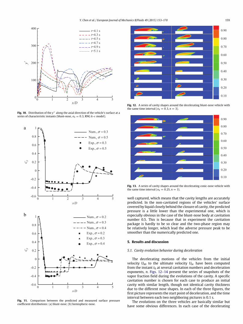
RNG k–ε model at a series of instants during this stage are shownin Fig. 10. The instants t = 4.3 s and t = 4.9 s are the momentswhen the cavity collapses, as indicated by the vapormass shown inFig. 5. The great velocity (or shear stress) induced by the collapsecan obviously increase the value of y+, as shown in Fig. 10 wherethe maximal y+ on these two curves are controlled in the rangeof y+ < 200–400. Meanwhile the minimal y+ on the curves of allthe instants in Fig. 10 are above the lower bound allowed by thecriterion.

4.4. Verification by experiment

The evolution of the cavities around the three vehicles is alsoinvestigated at their respective initial cavitation number in therange of 0.2 ≤ σ ≤ 0.5. Before the deceleration begins (t < 0.8 s),the pressure distributions along the vehicles’ surface are comparedwith the experimental data reported in the literature [1], as shownin Fig. 11.

The numerically obtained pressure distributions of the stablecavitating flows before deceleration are basically in accordancewith the experimental data. The values of the vapor pressure insidecavity and the adverse pressure near the closure of cavity are


Fig. 10. Distribution of the y+ along the axial direction of the vehicle’s surface at aseries of characteristic instants (blunt-nose, σ0 = 0.3, RNG k–ε model).

Fig. 11. Comparison between the predicted and measured surface pressurecoefficient distributions: (a) blunt-nose; (b) hemispheric-nose.

Fig. 12. A series of cavity shapes around the decelerating blunt-nose vehicle withthe same time interval (σ0 = 0.3, n = 3).

Fig. 13. A series of cavity shapes around the decelerating conic-nose vehicle withthe same time interval (σ0 = 0.25, n = 3).

well captured, which means that the cavity lengths are accuratelypredicted. In the non-cavitated regions of the vehicles’ surfacecovered by liquid closely behind the closure of cavity, the predictedpressure is a little lower than the experimental one, which isespecially obvious in the case of the blunt-nose body at cavitationnumber 0.5. This is because that in experiment the cavitationpackage is hardly to be so clear and the two-phase region maybe relatively longer, which lead the adverse pressure peak to besmoother than the numerically predicted one.

5. Results and discussion

5.1. Cavity evolution behavior during deceleration

The decelerating motions of the vehicles from the initialvelocity Ub0 to the ultimate velocity Ubt have been computedfrom the instant t0 at several cavitation numbers and decelerationexponents, n. Figs. 12–14 present the series of snapshots of thevapor fraction field during the evolutions of the cavity. A specificcavitation number is chosen for each case to produce an initialcavity with similar length, though not identical cavity thicknessdue to the different nose shapes. In each of the three figures, thefirst picture represents the start point of deceleration, and the timeinterval between each two neighboring pictures is 0.1 s.

The evolutions on the three vehicles are basically similar buthave some obvious differences. In each case of the decelerating


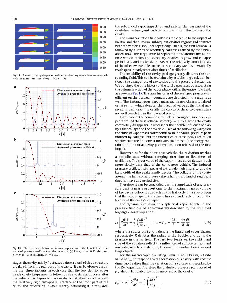
Fig. 14. A series of cavity shapes around the decelerating hemispheric-nose vehiclewith the same time interval (σ0 = 0.2, n = 3).

a

b

c

Fig. 15. The correlation between the total vapor mass in the flow field and theaveraged pressure coefficient on the boundary: (a) blunt, σ0 = 0.30; (b) conic,σ0 = 0.25; (c) hemispheric, σ0 = 0.20.

stages, the cavity axially fluctuates before a block of cloud structurebreaks off from the rear part of the cavity. It can be observed fromthe first three instants in each case that the low-density vaporinside cavity keeps moving leftwards due to its inertia force afterthe vehicle has begun to decelerate, but it shortly collide withthe relatively rigid two-phase interface at the front part of thecavity and reflects on it after slightly deforming it. Afterwards,

the rebounded vapor impacts on and inflates the rear part of thecavitation package, and leads to the non-uniform fluctuation of thecavity.

The cloud cavitation first collapses rapidly due to the impact ofinertia, and then several subsequent cavities regrow and contractnear the vehicles’ shoulder repeatedly. That is, the first collapse isfollowed by a series of secondary collapses caused by the unbal-anced flow. The large-scale of separated flow around the blunt-nose vehicle makes the secondary cavities to grow and collapseperiodically and endlessly. However, the relatively smooth nosesof the other two vehicles make the secondary cavities to graduallyreach quasi-steady state after times of oscillation.

The instability of the cavity package greatly disturbs the sur-rounding fluid. This can be explained by establishing a relation be-tween the change-rate of cavity size and the pressure fluctuation.We obtained the time history of the total vapormass by integratingthe volume fraction of the vapor phase within the entire flow field,as shown in Fig. 15. The time histories of the averaged pressure co-efficient on the upstream boundary are depicted in the graphs aswell. The instantaneous vapor mass, mv , is non-dimensionalizedusing mv,max, which denotes the maximal value at the initial mo-ment. In each case, the oscillation curves of these two quantitiesare well correlated in the reversed phase.

In the case of the conic-nose vehicle, a strong pressure peak ap-pears around the first collapse instant (t = 1.35 s) when the cavitycompletely disappears. It represents the notable influence of cav-ity’s first collapse on the flow field. Each of the following valleys onthe curve of vapormass corresponds to an individual pressure peakinduced by collapse, but the intensities of these peaks are muchsmaller than the first one. It indicates that most of the energy con-tained in the initial cavity package has been released in the firstimpact.

However, as for the blunt-nose vehicle, the cavitation reachesa periodic state without damping after four or five times ofoscillation. The crest value of the vapor–mass curve decays muchmore slowly than that of the conic-nose vehicle. The inducedpressure oscillates with peaks of extremely high intensity, and thebandwidth of the peaks hardly decays. The collapse of the cavityaround the hemispheric-nose vehicle has a third kind of regime. Itdoes not have any periodicity.

Therefore it can be concluded that the amplitude of any pres-sure peak is nearly proportional to the maximal mass or volumeof the cavity before it contracts in the last cycle. It is also proventhat the nose shape of the vehicle has a considerable effect on thefeature of the cavity’s collapse.

The dynamic evolution of a spherical vapor bubble in thepressure field can be approximately described by the simplifiedRayleigh–Plesset equation:

ρl

Rd2Rdt2

+32

dRdt

2

= pv − p∞ −2SR

−4µR

dRdt

(16)

where the subscripts l and v denote the liquid and vapor phases,respectively, R denotes the radius of the bubble, and p∞ is thepressure in the far field. The last two terms on the right-handside of the equation reflect the influences of surface tension andviscosity, which vanish in high Reynolds number flows aroundlarge objects.

For the macroscopic cavitating flows in equilibrium, a finitevalue of p∞ corresponds to the formation of a cavity with specificdimension, rather than the variation of its volume as described bythe R–P equation. Therefore the disturbed pressure p′

∞instead of

p∞ should be related to the change-rate of the cavity:

p′

∞∼ ρl

Rd2Rdt2

+32

dRdt

2 . (17)


1

0.25

0.5

0.75

50

-50

-25

0

25

-300

-200

-100

0

100

1 2 3 4 5 6

1 2 3 4 5 6

1 2 3 4 5 6

Fig. 16. The dimensionless equivalent radius of cavity and its change-rates (blunt-nose vehicle, σ0 = 0.30).

Here we assume that when the cavity has an irregular shape, itscollapse effect on the averaged pressure in the far field is similarwith that of a spherical cavity having the same volume. That is, theeffect is mainly determined by the volume of the cavity, providedthat the position is far enough away from the cavity.

Thus the averaged value of the disturbed pressure on theboundary can be used as the p′

∞, if the cavity is supposed to be

equivalent to a spherical bubble with the same volume. The equiv-alent radius, R, is defined using the instantaneous cavity volumeVC (t):

R(t) =

34VC (t)

π

13

. (18)

Therefore the following similarity exists between the averagedpressure coefficient and the change-rate of the specific kineticenergy of the collapse:

Cp ∼ E(R) =

Rd2Rdt2

+32

dRdt

2

12U2b0

. (19)

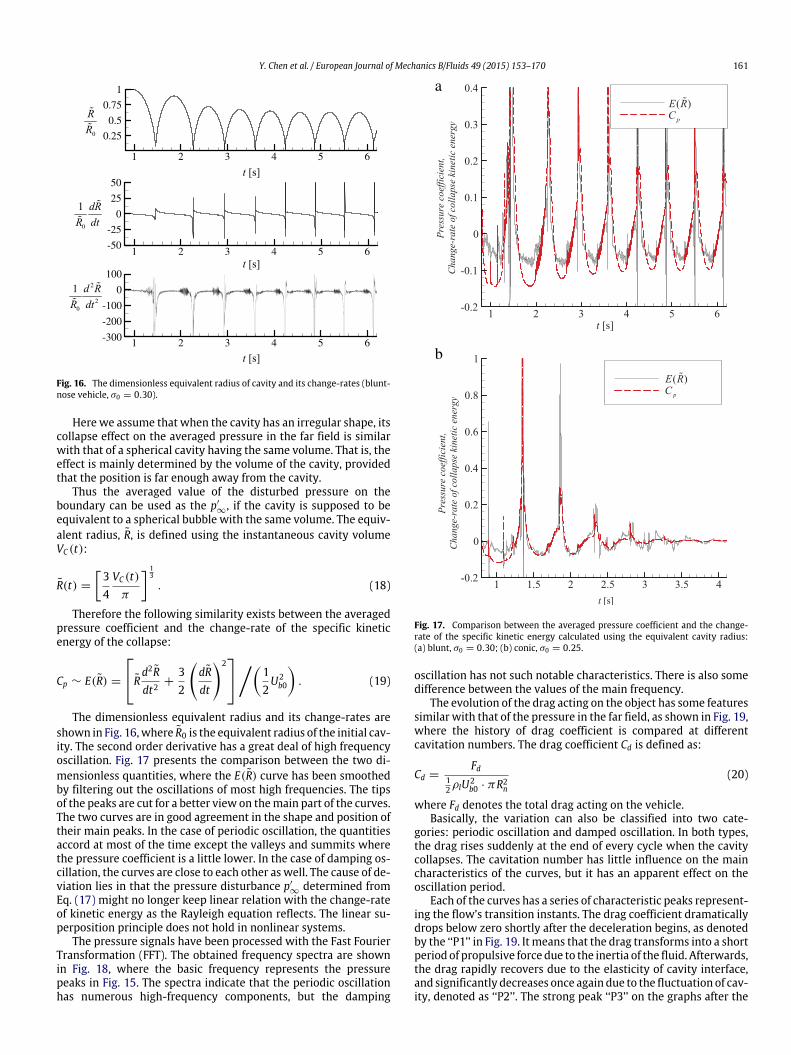
The dimensionless equivalent radius and its change-rates areshown in Fig. 16,where R0 is the equivalent radius of the initial cav-ity. The second order derivative has a great deal of high frequencyoscillation. Fig. 17 presents the comparison between the two di-mensionless quantities, where the E(R) curve has been smoothedby filtering out the oscillations of most high frequencies. The tipsof the peaks are cut for a better view on themain part of the curves.The two curves are in good agreement in the shape and position oftheir main peaks. In the case of periodic oscillation, the quantitiesaccord at most of the time except the valleys and summits wherethe pressure coefficient is a little lower. In the case of damping os-cillation, the curves are close to each other as well. The cause of de-viation lies in that the pressure disturbance p′

∞determined from

Eq. (17) might no longer keep linear relation with the change-rateof kinetic energy as the Rayleigh equation reflects. The linear su-perposition principle does not hold in nonlinear systems.

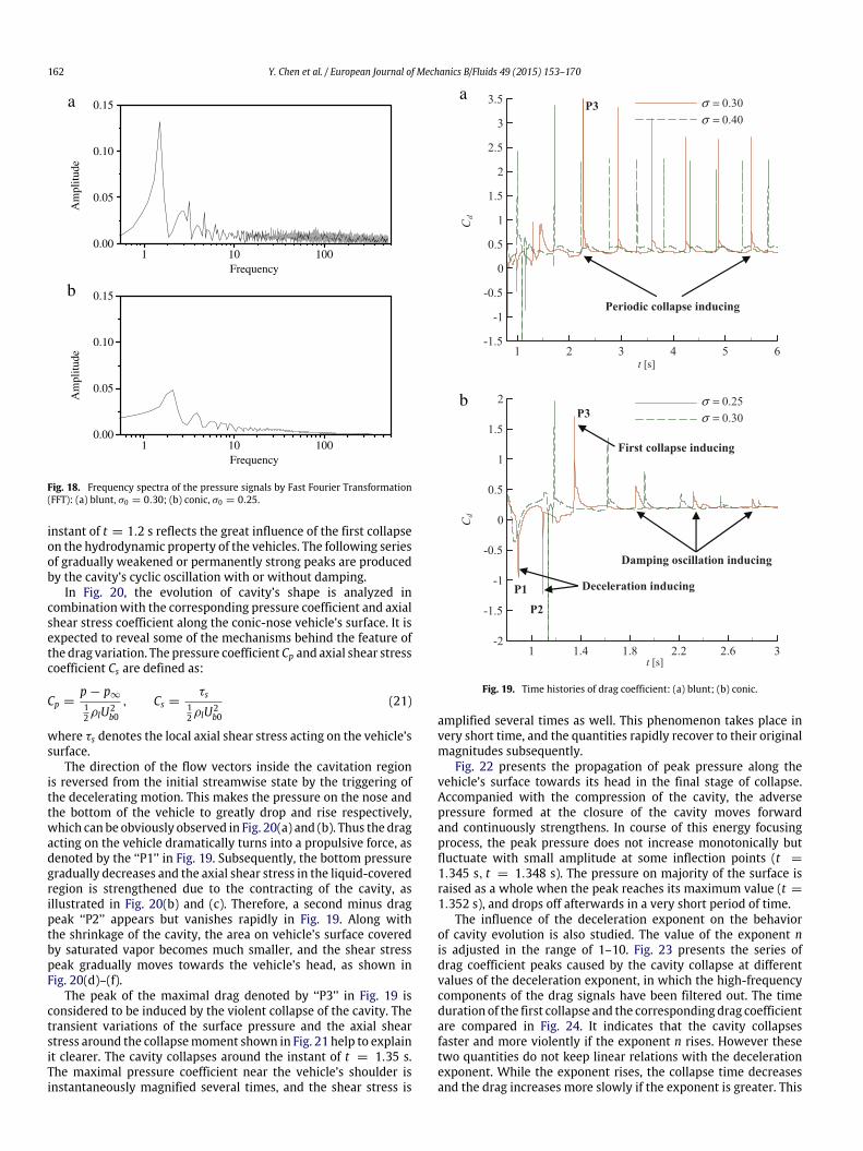
The pressure signals have been processed with the Fast FourierTransformation (FFT). The obtained frequency spectra are shownin Fig. 18, where the basic frequency represents the pressurepeaks in Fig. 15. The spectra indicate that the periodic oscillationhas numerous high-frequency components, but the damping

Fig. 17. Comparison between the averaged pressure coefficient and the change-rate of the specific kinetic energy calculated using the equivalent cavity radius:(a) blunt, σ0 = 0.30; (b) conic, σ0 = 0.25.

oscillation has not such notable characteristics. There is also somedifference between the values of the main frequency.

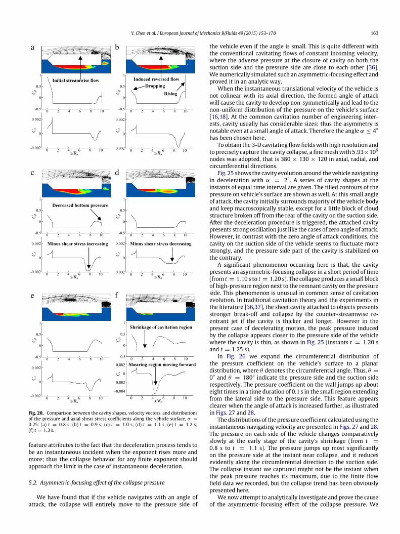
The evolution of the drag acting on the object has some featuressimilar with that of the pressure in the far field, as shown in Fig. 19,where the history of drag coefficient is compared at differentcavitation numbers. The drag coefficient Cd is defined as:

Cd =Fd

12ρlU2

b0 · πR2n

(20)

where Fd denotes the total drag acting on the vehicle.Basically, the variation can also be classified into two cate-

gories: periodic oscillation and damped oscillation. In both types,the drag rises suddenly at the end of every cycle when the cavitycollapses. The cavitation number has little influence on the maincharacteristics of the curves, but it has an apparent effect on theoscillation period.

Each of the curves has a series of characteristic peaks represent-ing the flow’s transition instants. The drag coefficient dramaticallydrops below zero shortly after the deceleration begins, as denotedby the ‘‘P1’’ in Fig. 19. It means that the drag transforms into a shortperiod of propulsive force due to the inertia of the fluid. Afterwards,the drag rapidly recovers due to the elasticity of cavity interface,and significantly decreases once again due to the fluctuation of cav-ity, denoted as ‘‘P2’’. The strong peak ‘‘P3’’ on the graphs after the


0.15

0.10

0.05

0.00

0.15

0.10

0.05

0.00

Am

plitu

deA

mpl

itude

1 10 100Frequency

1 10 100Frequency

a

b

Fig. 18. Frequency spectra of the pressure signals by Fast Fourier Transformation(FFT): (a) blunt, σ0 = 0.30; (b) conic, σ0 = 0.25.

instant of t = 1.2 s reflects the great influence of the first collapseon the hydrodynamic property of the vehicles. The following seriesof gradually weakened or permanently strong peaks are producedby the cavity’s cyclic oscillation with or without damping.

In Fig. 20, the evolution of cavity’s shape is analyzed incombination with the corresponding pressure coefficient and axialshear stress coefficient along the conic-nose vehicle’s surface. It isexpected to reveal some of the mechanisms behind the feature ofthe drag variation. The pressure coefficient Cp and axial shear stresscoefficient Cs are defined as:

Cp =p − p∞

12ρlU2

b0

, Cs =τs

12ρlU2

b0

(21)

where τs denotes the local axial shear stress acting on the vehicle’ssurface.

The direction of the flow vectors inside the cavitation regionis reversed from the initial streamwise state by the triggering ofthe decelerating motion. This makes the pressure on the nose andthe bottom of the vehicle to greatly drop and rise respectively,which can be obviously observed in Fig. 20(a) and (b). Thus the dragacting on the vehicle dramatically turns into a propulsive force, asdenoted by the ‘‘P1’’ in Fig. 19. Subsequently, the bottom pressuregradually decreases and the axial shear stress in the liquid-coveredregion is strengthened due to the contracting of the cavity, asillustrated in Fig. 20(b) and (c). Therefore, a second minus dragpeak ‘‘P2’’ appears but vanishes rapidly in Fig. 19. Along withthe shrinkage of the cavity, the area on vehicle’s surface coveredby saturated vapor becomes much smaller, and the shear stresspeak gradually moves towards the vehicle’s head, as shown inFig. 20(d)–(f).

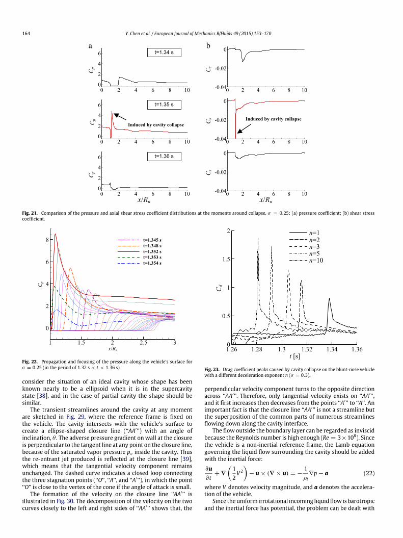
The peak of the maximal drag denoted by ‘‘P3’’ in Fig. 19 isconsidered to be induced by the violent collapse of the cavity. Thetransient variations of the surface pressure and the axial shearstress around the collapsemoment shown in Fig. 21 help to explainit clearer. The cavity collapses around the instant of t = 1.35 s.The maximal pressure coefficient near the vehicle’s shoulder isinstantaneously magnified several times, and the shear stress is

Fig. 19. Time histories of drag coefficient: (a) blunt; (b) conic.

amplified several times as well. This phenomenon takes place invery short time, and the quantities rapidly recover to their originalmagnitudes subsequently.

Fig. 22 presents the propagation of peak pressure along thevehicle’s surface towards its head in the final stage of collapse.Accompanied with the compression of the cavity, the adversepressure formed at the closure of the cavity moves forwardand continuously strengthens. In course of this energy focusingprocess, the peak pressure does not increase monotonically butfluctuate with small amplitude at some inflection points (t =

1.345 s, t = 1.348 s). The pressure on majority of the surface israised as a whole when the peak reaches its maximum value (t =

1.352 s), and drops off afterwards in a very short period of time.The influence of the deceleration exponent on the behavior

of cavity evolution is also studied. The value of the exponent nis adjusted in the range of 1–10. Fig. 23 presents the series ofdrag coefficient peaks caused by the cavity collapse at differentvalues of the deceleration exponent, in which the high-frequencycomponents of the drag signals have been filtered out. The timeduration of the first collapse and the corresponding drag coefficientare compared in Fig. 24. It indicates that the cavity collapsesfaster and more violently if the exponent n rises. However thesetwo quantities do not keep linear relations with the decelerationexponent. While the exponent rises, the collapse time decreasesand the drag increases more slowly if the exponent is greater. This


a

c

e

b

d

f

Fig. 20. Comparison between the cavity shapes, velocity vectors, and distributionsof the pressure and axial shear stress coefficients along the vehicle surface, σ =

0.25: (a) t = 0.8 s; (b) t = 0.9 s; (c) t = 1.0 s; (d) t = 1.1 s; (e) t = 1.2 s;(f) t = 1.3 s.

feature attributes to the fact that the deceleration process tends tobe an instantaneous incident when the exponent rises more andmore; thus the collapse behavior for any finite exponent shouldapproach the limit in the case of instantaneous deceleration.

5.2. Asymmetric-focusing effect of the collapse pressure

We have found that if the vehicle navigates with an angle ofattack, the collapse will entirely move to the pressure side of

the vehicle even if the angle is small. This is quite different withthe conventional cavitating flows of constant incoming velocity,where the adverse pressure at the closure of cavity on both thesuction side and the pressure side are close to each other [36].We numerically simulated such an asymmetric-focusing effect andproved it in an analytic way.

When the instantaneous translational velocity of the vehicle isnot colinear with its axial direction, the formed angle of attackwill cause the cavity to develop non-symmetrically and lead to thenon-uniform distribution of the pressure on the vehicle’s surface[16,18]. At the common cavitation number of engineering inter-ests, cavity usually has considerable sizes; thus the asymmetry isnotable even at a small angle of attack. Therefore the angle α ≤ 4°has been chosen here.

To obtain the 3-D cavitating flow fieldswith high resolution andto precisely capture the cavity collapse, a finemeshwith 5.93×106

nodes was adopted, that is 380 × 130 × 120 in axial, radial, andcircumferential directions.

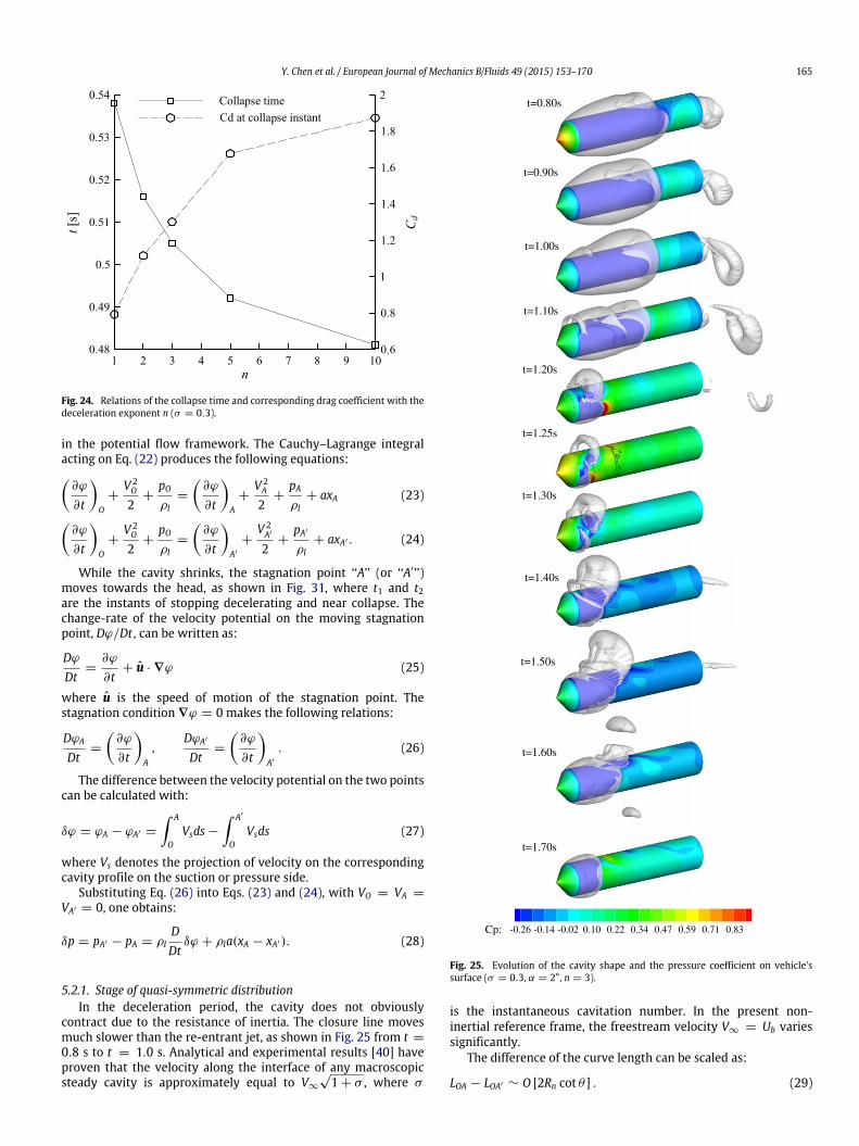
Fig. 25 shows the cavity evolution around the vehicle navigatingin deceleration with α = 2°. A series of cavity shapes at theinstants of equal time interval are given. The filled contours of thepressure on vehicle’s surface are shown as well. At this small angleof attack, the cavity initially surroundsmajority of the vehicle bodyand keep macroscopically stable, except for a little block of cloudstructure broken off from the rear of the cavity on the suction side.After the deceleration procedure is triggered, the attached cavitypresents strong oscillation just like the cases of zero angle of attack.However, in contrast with the zero angle of attack conditions, thecavity on the suction side of the vehicle seems to fluctuate morestrongly, and the pressure side part of the cavity is stabilized onthe contrary.

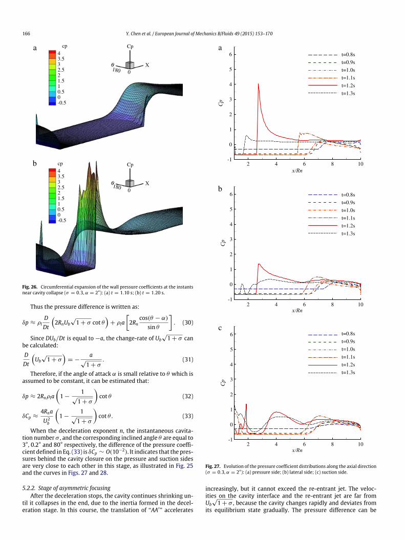
A significant phenomenon occurring here is that, the cavitypresents an asymmetric-focusing collapse in a short period of time(from t = 1.10 s to t = 1.20 s). The collapse produces a small blockof high-pressure region next to the remnant cavity on the pressureside. This phenomenon is unusual in common sense of cavitationevolution. In traditional cavitation theory and the experiments inthe literature [36,37], the sheet cavity attached to objects presentsstronger break-off and collapse by the counter-streamwise re-entrant jet if the cavity is thicker and longer. However in thepresent case of decelerating motion, the peak pressure inducedby the collapse appears closer to the pressure side of the vehiclewhere the cavity is thin, as shown in Fig. 25 (instants t = 1.20 sand t = 1.25 s).

In Fig. 26 we expand the circumferential distribution ofthe pressure coefficient on the vehicle’s surface to a planardistribution, where θ denotes the circumferential angle. Thus, θ =

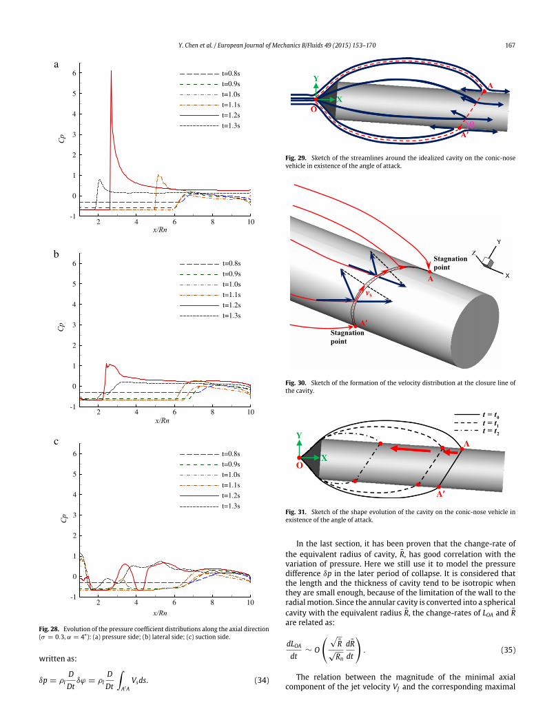
0° and θ = 180° indicate the pressure side and the suction siderespectively. The pressure coefficient on the wall jumps up abouteight times in a time duration of 0.1 s in the small region extendingfrom the lateral side to the pressure side. This feature appearsclearer when the angle of attack is increased further, as illustratedin Figs. 27 and 28.

The distributions of the pressure coefficient calculated using theinstantaneous navigating velocity are presented in Figs. 27 and 28.The pressure on each side of the vehicle changes comparativelyslowly at the early stage of the cavity’s shrinkage (from t =

0.8 s to t = 1.1 s). The pressure jumps up most significantlyon the pressure side at the instant near collapse, and it reducesevidently along the circumferential direction to the suction side.The collapse instant we captured might not be the instant whenthe peak pressure reaches its maximum, due to the finite flowfield data we recorded, but the collapse trend has been obviouslypresented here.

We now attempt to analytically investigate and prove the causeof the asymmetric-focusing effect of the collapse pressure. We


Fig. 21. Comparison of the pressure and axial shear stress coefficient distributions at the moments around collapse, σ = 0.25: (a) pressure coefficient; (b) shear stresscoefficient.

Fig. 22. Propagation and focusing of the pressure along the vehicle’s surface forσ = 0.25 (in the period of 1.32 s < t < 1.36 s).

consider the situation of an ideal cavity whose shape has beenknown nearly to be a ellipsoid when it is in the supercavitystate [38], and in the case of partial cavity the shape should besimilar.

The transient streamlines around the cavity at any momentare sketched in Fig. 29, where the reference frame is fixed onthe vehicle. The cavity intersects with the vehicle’s surface tocreate a ellipse-shaped closure line (‘‘AA′’’) with an angle ofinclination, θ . The adverse pressure gradient on wall at the closureis perpendicular to the tangent line at any point on the closure line,because of the saturated vapor pressure pv inside the cavity. Thusthe re-entrant jet produced is reflected at the closure line [39],which means that the tangential velocity component remainsunchanged. The dashed curve indicates a closed loop connectingthe three stagnation points (‘‘O’’, ‘‘A’’, and ‘‘A′’’), in which the point‘‘O’’ is close to the vertex of the cone if the angle of attack is small.

The formation of the velocity on the closure line ‘‘AA′’’ isillustrated in Fig. 30. The decomposition of the velocity on the twocurves closely to the left and right sides of ‘‘AA′’’ shows that, the

Fig. 23. Drag coefficient peaks caused by cavity collapse on the blunt-nose vehiclewith a different deceleration exponent n (σ = 0.3).

perpendicular velocity component turns to the opposite directionacross ‘‘AA′’’. Therefore, only tangential velocity exists on ‘‘AA′’’,and it first increases then decreases from the points ‘‘A′’’ to ‘‘A’’. Animportant fact is that the closure line ‘‘AA′’’ is not a streamline butthe superposition of the common parts of numerous streamlinesflowing down along the cavity interface.

The flow outside the boundary layer can be regarded as inviscidbecause the Reynolds number is high enough (Re = 3×108). Sincethe vehicle is a non-inertial reference frame, the Lamb equationgoverning the liquid flow surrounding the cavity should be addedwith the inertial force:

∂u∂t

+ ∇

12V 2

− u × (∇ × u) = −1ρl

∇p − a (22)

where V denotes velocity magnitude, and a denotes the accelera-tion of the vehicle.

Since theuniform irrotational incoming liquid flow is barotropicand the inertial force has potential, the problem can be dealt with


Fig. 24. Relations of the collapse time and corresponding drag coefficient with thedeceleration exponent n (σ = 0.3).

in the potential flow framework. The Cauchy–Lagrange integralacting on Eq. (22) produces the following equations:

∂ϕ

∂t

O

+V 2O

2+

pOρl

=

∂ϕ

∂t

A+

V 2A

2+

pAρl

+ axA (23)∂ϕ

∂t

O

+V 2O

2+

pOρl

=

∂ϕ

∂t

A′

+V 2A′

2+

pA′

ρl+ axA′ . (24)

While the cavity shrinks, the stagnation point ‘‘A’’ (or ‘‘A′’’)moves towards the head, as shown in Fig. 31, where t1 and t2are the instants of stopping decelerating and near collapse. Thechange-rate of the velocity potential on the moving stagnationpoint, Dϕ/Dt , can be written as:

Dϕ

Dt=

∂ϕ

∂t+ u · ∇ϕ (25)

where u is the speed of motion of the stagnation point. Thestagnation condition ∇ϕ = 0 makes the following relations:

DϕA

Dt=

∂ϕ

∂t

A,

DϕA′

Dt=

∂ϕ

∂t

A′

. (26)

The difference between the velocity potential on the two pointscan be calculated with:

δϕ = ϕA − ϕA′ =

A

OVsds −

A′

OVsds (27)

where Vs denotes the projection of velocity on the correspondingcavity profile on the suction or pressure side.

Substituting Eq. (26) into Eqs. (23) and (24), with VO = VA =

VA′ = 0, one obtains:

δp = pA′ − pA = ρlDDt

δϕ + ρla(xA − xA′). (28)

5.2.1. Stage of quasi-symmetric distributionIn the deceleration period, the cavity does not obviously

contract due to the resistance of inertia. The closure line movesmuch slower than the re-entrant jet, as shown in Fig. 25 from t =

0.8 s to t = 1.0 s. Analytical and experimental results [40] haveproven that the velocity along the interface of any macroscopicsteady cavity is approximately equal to V∞

√1 + σ , where σ

t=0.80s

t=0.90s

t=1.00s

t=1.10s

t=1.20s

t=1.25s

t=1.30s

t=1.40s

t=1.50s

t=1.60s

t=1.70s

Cp: -0.26 -0.14 -0.02 0.10 0.22 0.34 0.47 0.59 0.71 0.83

Fig. 25. Evolution of the cavity shape and the pressure coefficient on vehicle’ssurface (σ = 0.3, α = 2°, n = 3).

is the instantaneous cavitation number. In the present non-inertial reference frame, the freestream velocity V∞ = Ub variessignificantly.

The difference of the curve length can be scaled as:

LOA − LOA′ ∼ O [2Rn cot θ ] . (29)


cp43.532.521.510.50-0.5

cp43.532.521.510.50-0.5

Cp

X180 0

θ

Cp

X180 0

θ

a

b

Fig. 26. Circumferential expansion of the wall pressure coefficients at the instantsnear cavity collapse (σ = 0.3, α = 2°): (a) t = 1.10 s; (b) t = 1.20 s.

Thus the pressure difference is written as:

δp ≈ ρlDDt

2RnUb

√1 + σ cot θ

+ ρla

2Rn

cos(θ − α)

sin θ

. (30)

Since DUb/Dt is equal to −a, the change-rate of Ub√1 + σ can

be calculated:DDt

Ub

√1 + σ

= −

a√1 + σ

. (31)

Therefore, if the angle of attack α is small relative to θ which isassumed to be constant, it can be estimated that:

δp ≈ 2Rnρla1 −

1√1 + σ

cot θ (32)

δCp ≈4RnaU2b

1 −

1√1 + σ

cot θ. (33)

When the deceleration exponent n, the instantaneous cavita-tion number σ , and the corresponding inclined angle θ are equal to3°, 0.2° and 80° respectively, the difference of the pressure coeffi-cient defined in Eq. (33) is δCp ∼ O(10−2). It indicates that the pres-sures behind the cavity closure on the pressure and suction sidesare very close to each other in this stage, as illustrated in Fig. 25and the curves in Figs. 27 and 28.

5.2.2. Stage of asymmetric focusingAfter the deceleration stops, the cavity continues shrinking un-

til it collapses in the end, due to the inertia formed in the decel-eration stage. In this course, the translation of ‘‘AA′’’ accelerates

6

5

4

3

2

1

0

-12 4 6 8 10

6

5

4

3

2

1

0

-12 4 6 8 10

6

5

4

3

2

1

0

-12 4 6 8 10

t=0.8s

t=0.9s

t=1.0s

t=1.1s

t=1.2s

t=1.3s

t=0.8s

t=0.9s

t=1.0s

t=1.1s

t=1.2s

t=1.3s

t=0.8s

t=0.9s

t=1.0s

t=1.1s

t=1.2s

t=1.3s

a

b

c

Fig. 27. Evolution of the pressure coefficient distributions along the axial direction(σ = 0.3, α = 2°): (a) pressure side; (b) lateral side; (c) suction side.

increasingly, but it cannot exceed the re-entrant jet. The veloc-ities on the cavity interface and the re-entrant jet are far fromUb

√1 + σ , because the cavity changes rapidly and deviates from

its equilibrium state gradually. The pressure difference can be


6

5

4

3

2

1

0

-12 4 6 8 10

6

5

4

3

2

1

0

-12 4 6 8 10

6

5

4

3

2

1

0

-12 4 6 8 10

t=0.8s

t=0.9s

t=1.0s

t=1.1s

t=1.2s

t=1.3s

t=0.8s

t=0.9s

t=1.0s

t=1.1s

t=1.2s

t=1.3s

t=0.8s

t=0.9s

t=1.0s

t=1.1s

t=1.2s

t=1.3s

a

b

c

Fig. 28. Evolution of the pressure coefficient distributions along the axial direction(σ = 0.3, α = 4°): (a) pressure side; (b) lateral side; (c) suction side.

written as:

δp = ρlDDt

δϕ = ρlDDt

A′A

Vsds. (34)

Fig. 29. Sketch of the streamlines around the idealized cavity on the conic-nosevehicle in existence of the angle of attack.

Fig. 30. Sketch of the formation of the velocity distribution at the closure line ofthe cavity.

Fig. 31. Sketch of the shape evolution of the cavity on the conic-nose vehicle inexistence of the angle of attack.

In the last section, it has been proven that the change-rate ofthe equivalent radius of cavity, R, has good correlation with thevariation of pressure. Here we still use it to model the pressuredifference δp in the later period of collapse. It is considered thatthe length and the thickness of cavity tend to be isotropic whenthey are small enough, because of the limitation of the wall to theradialmotion. Since the annular cavity is converted into a sphericalcavity with the equivalent radius R, the change-rates of LOA and Rare related as:

dLOAdt

∼ O

R

√Rn

dRdt

. (35)

The relation between the magnitude of the minimal axialcomponent of the jet velocity VJ and the corresponding maximal


velocity on the closure line is:

Vs,max = VJ,mincos(θ − α)

cos(π − 2θ + α). (36)

This equation can also be expressed as Vs,max = C(θ)VJ,min,where the coefficient C(θ) decreases alongwith the reduction ofα.The integration of the velocity along the closure line is in scalewiththe mean velocity Vs or the maximal velocity Vs,max, consideringthat LA′A = 2Rn/ sin θ :

A′AVsds ∼ O(VsRn) ∼ O(Vs,maxRn). (37)

The re-entrant jet reflects on the closure line ‘‘AA′’’; thus VJ,minshould be greater than or at least not be lower than dLOA/dt . Thefollowing relation exists:

VJ,min ≈

dLOAdt

. (38)

After putting all the above-mentioned equations together, thepressure difference between ‘‘A′’’ and ‘‘A’’ is in proportional relationto a composite expression of the equivalent radius R and itschange-rates:

δp ∼ ρl

Rn

DDt

R

dRdt

= −ρl

Rn

Rd2Rdt2

+1

2R

dRdt

2 . (39)

The R satisfies the Rayleigh equation as Eq. (16) neglecting theviscous and surface tension terms. It is easy to obtain the change-rates of R:

dRdt

= −

23p∞ − pv

ρl

R30

R3− 1

(40)

d2Rdt2

= −p∞ − pv

ρl

R30

R4. (41)

By substituting Eqs. (40) and (41) into Eq. (39), we findthe final expression establishing the relationship between thepressure difference and the equivalent radius which is contractingacceleratingly:

δp ∼13(p∞ − pv)

Rn

R

2

R0

R

3

+ 1

. (42)

The corresponding difference of pressure coefficient can beestimated as follows, given that R0/R ≫ 1:

δCp ∼23σ

Rn

R

R0

R

3

. (43)

Eq. (42) or Eq. (43) gives an explanation of the asymmetric-focusing effect of the pressure at the closure during the collapse. Itindicates that the induced pressure on the pressure side increasesabout O(R−7/2) times faster than that on the suction side when Rdecreases. It provides an insight into the mechanism behind theresult that has been illustrated in Figs. 27 and 28. In Eqs. (42) and(43), the influence of the angle of attack represented by the C(θ) inEq. (36) is implicitly involved in the proportional coefficient. Thatis, δCp is greater when α is larger.

Fig. 32. The coefficient of moment of force with respect to the vehicle’s centroid(xc/Rn = 5.5, yc = 0, zc = 0).

Fig. 33. The influence of the angle of attack on the dimensionless vapor mass incavity.

The modeling and deduction made here are grounded on thehypothesis of ideal cavity shape and the simplification using thepotential flow theory. Nevertheless, it is still effective in reflectingthe main feature of the asymmetric pressure. The irregularity ofcavity and the viscosity in real flows have some effects on theintensity and position of the peak pressure, but the influence hasnot been known yet and will not be investigated here.

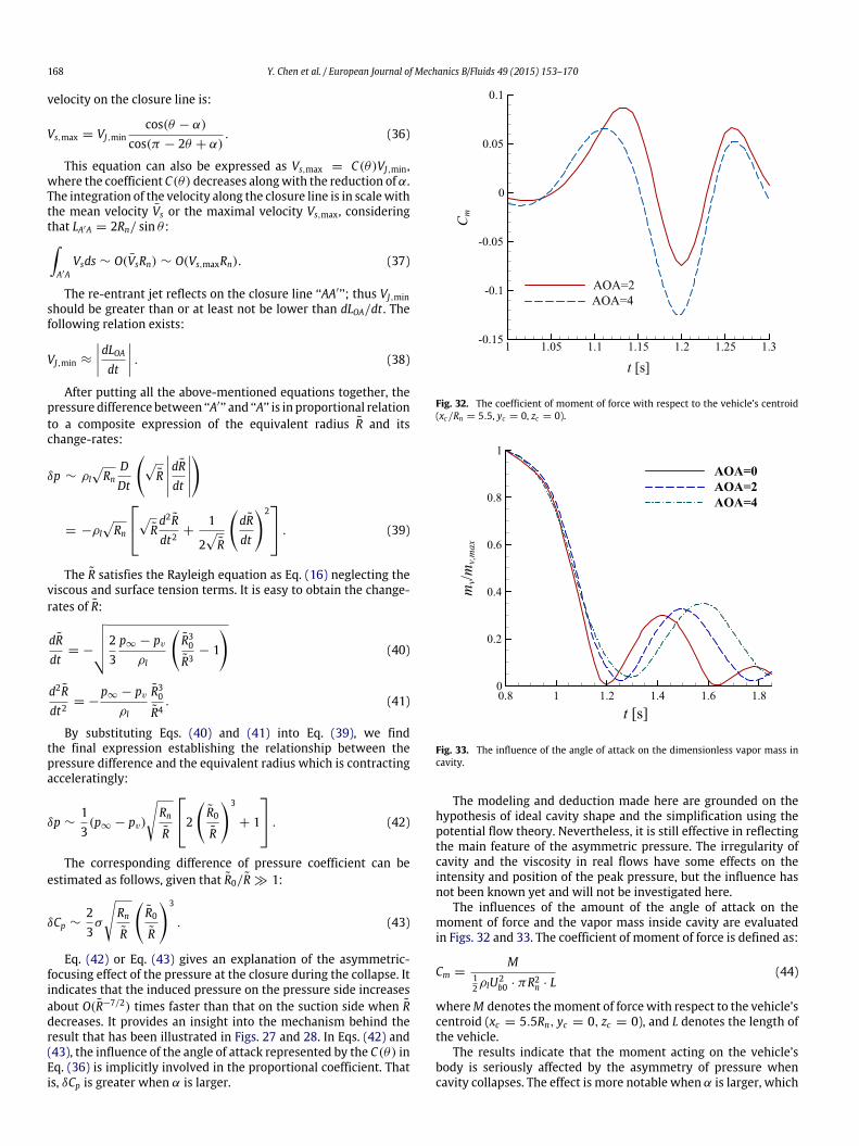
The influences of the amount of the angle of attack on themoment of force and the vapor mass inside cavity are evaluatedin Figs. 32 and 33. The coefficient of moment of force is defined as:

Cm =M

12ρlU2

b0 · πR2n · L

(44)

whereM denotes themoment of forcewith respect to the vehicle’scentroid (xc = 5.5Rn, yc = 0, zc = 0), and L denotes the length ofthe vehicle.

The results indicate that the moment acting on the vehicle’sbody is seriously affected by the asymmetry of pressure whencavity collapses. The effect is more notable when α is larger, which


is consistent with the proportional coefficient C(θ) in Eq. (36). Theevolution of the vapor mass implies that the cavity collapses moreslowly for a relatively larger angle of attack. The cause of it liesin that, the time duration of the collapse is mainly determinedby the suction side where the cavity shrinks more slowly for alarger angle of attack, because the induced high pressure whichconversely pushes the cavity is focused to the pressure side morewhen α is larger.

6. Conclusion

In the present work, the collapse regimes of the cavitationoccurring on the submerged vehicles navigating with continuousdeceleration were numerically investigated. A cavitation modelbased on the transport equation of phase fraction was combinedwith the pressure–velocity–density coupling algorithm to simulatethe cavitating flows. The mesh convergence analysis was firstcarried out to choose suitable computational mesh. Afterwards thetime step, turbulence model, and fundamental numerical resultswere verified and validated by experimental data.

The evolutions of the cavities around kinds of vehicles exhibitdifferent features. The collapse of cavity is induced by thedeceleration after times of fluctuation, and the first collapsereleasing most of the energy is followed by a series of secondarycollapses. The collapse process can be classified into two types:periodic oscillation and damped oscillation. In each type theevolution of the total mass of vapor in cavity is found to havestrict correlation with the pressure oscillation in the far field. Thetwo types are different in the intensity and the bandwidth of thepressure peaks. By defining the equivalent radius of cavity, weintroduce the specific kinetic energy of collapse and demonstratethat its change-rate is in good agreement with the pressuredisturbance. It is also found that the drag acting on the vehiclespresents corresponding oscillations induced by the collapse.Through comparative analysis with the velocity field and the stressdistribution along the body, it has been proven that the collapsecan produce extremely high values of pressure and shear stressinstantaneously. The series of peaks of drag coefficient presents thetypical feature of the periodic or damped collapse of cavity.

We numerically investigated the influence of the angle of attackon the collapse of the cavity. The result shows that when thevehicle decelerates, an asymmetric-focusing effect of the pressureinduced by collapse occurs on its pressure side even if the angleis small. The pressure at the closure of the cavity on the pressureside and that on suction side are very close to each other in thedeceleration stage, while it rapidly focuses to the pressure side inthe subsequent stage of uniform navigation speed. We analyticallyproved such an asymmetric-focusing effect using the potentialflow theory. The mathematical model and method we proposedshow good capability in reflecting the evolution of the pressuredifference between both sides of the vehicle.

Acknowledgments

This project is supported by the National Nature Science Foun-dation of China (Grant No. 11472174, 11102110 and 11372185)and the Ph.D. Programs Foundation of Ministry of Education ofChina (Grant No. 20110073120009). Their financial supports aregratefully acknowledged.

References

[1] H. Rouse, J.S. McNown, Cavitation and Pressure Distribution, Head Forms atZero Angle of Yaw, in: Studies in Engineering Bulletin, vol. 32, State Universityof Iowa, 1948.

[2] Y.N. Savchenko, Supercavitation—problems and perspectives, in: Proceedingsof the 4th International Symposium on Cavitation, California, USA, 2001.

[3] Y.D. Vlasenko, Experimental investigation of supercavitation flow regimesat subsonic and transonic speeds, in: Proceedings of the 5th InternationalSymposium on Cavitation, Osaka, Japan, 2003.

[4] B. Huang, G. Wang, X. Quan, et al., Study on the unsteady cavitating flowdynamic characteristics around a 0-caliber ogive revolution body, J. Exp. FluidMech. 25 (2) (2011) 22–28.

[5] A. Kubota, H. Kato, H. Yamaguchi, A new modeling of cavitating flows: anumerical study of unsteady cavitation on a hydrofoil section, J. Fluid Mech.240 (7) (1992) 59–96.

[6] G.H. Schnerr, J. Sauer, Physical and numerical modeling of unsteady cavitationdynamics, in: Proceedings of the 4th International Conference on MultiphaseFlow, New Orleans, USA, 2001.

[7] M. Frobenius, R. Schilling, R. Bachert, et al. Three-dimensional, unsteadycavitation effects on a single hydrofoil and in a radial pump—measurementsand numerical simulations, partial two: numerical simulation, in: Proceedingsof the 5th International Symposium on Cavitation, Osaka, Japan, 2003.

[8] Y. Delannoy, J.L. Kueny, Two-phase flow approach in unsteady cavitationmodeling, in: ASME Cavitation and Multiphase Flow Forum, Toronto, Canada,1990.

[9] O. Coutier-Delgosha, R. Fortes-Patella, J.L. Reboud, Evaluation of the turbulencemodel influence on the numerical simulations of unsteady cavitation, J. FluidsEng. 125 (1) (2003) 38–45.

[10] R.S. Byeong, Y. Satoru, Y. Xin, Application of preconditioning method togas–liquid twophase flow computations, J. Fluids Eng. 126 (4) (2004) 605–612.

[11] E. Goncalves, Numerical study of unsteady turbulent cavitating flows, Eur. J.Mech. B Fluids 30 (1) (2011) 26–40.

[12] C.L. Merkle, J.Z. Feng, P.E.O. Buelow, Computational modeling of the dynamicsof sheet cavitation, in: Proceedings of the 3rd International Symposium onCavitation, Grenoble, France, 1998.

[13] R.F. Kunz, D.A. Boger, D.R.A. Stinebring, Preconditioned Navier–Stokesmethodfor two-phase flows with application to cavitation prediction, Comput. Fluids29 (8) (2000) 849–875.

[14] W.X. Yuan, J. Sauer, G.H. Schnerr, Modeling and computation of unsteadycavitation flows in injection nozzles, Mec. Ind. (2) (2001) 383–394.

[15] A.K. Singhal, M.M. Athavale, H.Y. Li, et al., Mathematical basis and validationof the full cavitation model, J. Fluids Eng. 124 (3) (2002) 617–624.

[16] J.W. Lindau, R.F. Kunz, D.A. Boger, et al., High Reynolds number, unsteady,multiphase CFD modeling of cavitating flows, J. Fluids Eng. 124 (2002)607–616.

[17] D.H. Kim, W.G. Park, C.M. Jung, Numerical simulation of cavitating flow pastaxisymmetric body, J. Naval Arch. Ocean Eng. (4) (2012) 256–266.

[18] F.M. Owis, A.H. Nayfeh, Numerical simulation of 3-D incompressible, multi-phase flows over cavitating projectiles, Eur. J. Mech. B Fluids 23 (2004)339–351.

[19] I. Senocak, W. Shyy, A pressure-based method for turbulent cavitating flowcomputations, J. Comput. Phys. 176 (2002) 363–383.

[20] E. Goncalves, Numerical study of expansion tube problems: toward thesimulation of cavitation, Comput. Fluids 72 (2013) 1–19.

[21] E. Goncalves, B. Charriere, Modelling for isothermal cavitation with a fourequation model, Int. J. Multiph. Flow 59 (2014) 54–72.

[22] T. Barberon, P. Helluy, Finite volume simulation of cavitating flows, Comput.Fluids 34 (7) (2005) 832–858.

[23] S. Gavrilyuk, R. Saurel, Mathematical and numerical modeling of two-phasecompressible flows with micro-inertia, J. Comput. Phys. 175 (2002) 326–360.

[24] R. Saurel, F. Petitpas, R. Abgrall, Modelling phase transition in metastableliquids: application to cavitating and flashing flows, J. Fluid Mech. 607 (2008)313–350.

[25] F. Petitpas, J. Massoni, R. Saurel, E. Lapebie, L. Munier, Diffuse interface modelfor high speed cavitating underwater systems, Int. J. Multiph. Flow 35 (8)(2009) 747–759.

[26] F. Petitpas, R. Saurel, B.K. Ahn, S. Ko, Modelling cavitating flow aroundunderwater missiles, Int. J. Naval Arch. Ocean Eng. 3 (4) (2014) 263–273.

[27] J.P. Franc, J.M. Michel, Fundamentals of Cavitation, Kluwer AcademicPublishers, 2004.

[28] P.J. Zwart, A.G. Gerber, T. Belamri, A two-phase flow model for predictingcavitation dynamics, in: Proceedings of the 5th International Conference onMultiphase Flow, Yokohama, Japan, 2004.

[29] M. Morgut, E. Nobile, I. Bilus, Comparison of mass transfer models for thenumerical prediction of sheet cavitation around a hydrofoil, Int. J. Multiph.Flow 37 (2011) 620–626.

[30] M. Morgut, E. Nobile, Numerical Predictions of cavitating flow around modelscale propellers by CFD and advanced model calibration, Int. J. Rotating Mach.(2012) ID 618180.

[31] I. Demirdzic, Z. Lilek,M. Peric, A collocated finite volumemethod for predictingflows at all speeds, Internat. J. Numer. Methods Fluids 16 (1993) 1029–1050.

[32] K. Akagawa, Gas–Liquid Two-Phase Flow, Corona Publication, Tokyo, 1974.[33] B.R. Shin, Y. Iwata, T. Ikohagi, Numerical simulation of unsteady cavitating

flows using a homogeneous equilibrium model, Comput. Mech. 30 (2003)388–395.

[34] Y. Saito, R. Takami, I. Nakamori, et al., Numerical analysis of unsteady behaviorof cloud cavitation around a NACA0015 foil, Comput. Mech. 40 (1) (2007)85–96.

http://refhub.elsevier.com/S0997-7546(14)00135-6/sbref1




























[35] W. Anderson, D.L. Bonhus, An implicit upwind algorithm for computingturbulent flows on unstructured grids, Comput. Fluids 23 (1) (1994) 1–21.

[36] M. Callenaere, J.P. Franc, J.M. Michel, et al., The cavitation instability inducedby the development of a re-entrant jet, J. Fluid Mech. 444 (2001) 223–256.

[37] J.P. Franc, Partial cavity instabilities and re-entrant jet, in: Proceedings of the4th International Symposium on Cavitation, California, USA, 2001: Lecture002.

[38] Y.N. Savchenko, Y.D. Vlasenko, V.N. Semenenko, Experimental study of high-speed cavitated flows, Int. J. Fluid Mech. Res. 26 (3) (1999) 365–374.

[39] K.R. Laberteaux, S.L. Ceccio, Partial cavity flows. Part 2. Cavities forming on testobjects with spanwise variation, J. Fluid Mech. 431 (2001) 43–63.

[40] T.M. Pham, F. Larrarte, D.H. Fruman, Investigation of unsteady sheetcavitation and cloud cavitation mechanisms, J. Fluids Eng. 121 (1999)289–296.






Documents

Numerical investigation on the cavitation collapse regime around the submerged vehicles navigating with deceleration