Computers & Fluids 39 (2010) 1529–1541

Contents lists available at ScienceDirect

Computers & Fluids

journal homepage: www.elsevier .com/ locate /compfluid

Numerical investigations on dynamic stall of low Reynolds number flowaround oscillating airfoils q

Shengyi Wang a,b,*,1, Derek B. Ingham b, Lin Ma b, Mohamed Pourkashanian b, Zhi Tao a

a School of Jet Propulsion, Beijing University of Aeronautics and Astronautics, Beijing 100191, Chinab Centre for CFD, University of Leeds, Leeds LS2 9JT, United Kingdom

a r t i c l e i n f o

Article history:Received 24 August 2009Received in revised form 18 January 2010Accepted 11 May 2010Available online 15 May 2010

Keywords:Dynamic stallLow Reynolds numberOscillating bladeAerodynamicsSST k �x turbulence modelVAWT

0045-7930/$ - see front matter � 2010 Elsevier Ltd. Adoi:10.1016/j.compfluid.2010.05.004

q This paper is a collaborative effort.* Corresponding author at: Centre for CFD, Univer

United Kingdom. Tel.: +44 (0)113 343 2569; fax: +44E-mail addresses: presw@leeds.ac.uk, gmwsy@163

leeds.ac.uk (D.B. Ingham), L.Ma@leeds.ac.uk (L. Ma), M(M. Pourkashanian), tao_zhi@buaa.edu.cn (Z. Tao).

1 Mr. Shengyi Wang is currently a visiting PhD studeUniversity of Leeds, United Kingdom.

a b s t r a c t

This paper presents a 2D computational investigation on the dynamic stall phenomenon associated withunsteady flow around the NACA0012 airfoil at low Reynolds number (Rec � 105). Two sets of oscillatingpatterns with different frequencies, mean oscillating angles and amplitudes are numerically simulatedusing Computational Fluid Dynamics (CFD), and the results obtained are validated against the corre-sponding published experimental data. It is concluded that the CFD prediction captures well the vor-tex-shedding predominated flow structure which is experimentally obtained and the resultsquantitatively agree well with the experimental data, except when the blade is at a very high angle ofattack.

� 2010 Elsevier Ltd. All rights reserved.

1. Introduction

With the depletion of fossil fuel energy, and the increasingacknowledgement of the importance of developing environmen-tally friendly energy resources, the wind turbine, as the main tech-nology to extract energy from wind, has been increasinglyinvestigated. From the perspective of urban applications, VerticalAxis Wind Turbines (VAWTs) have many advantages over thewidely used conventional Horizontal Axis Wind Turbines (HAWTs)[1–4]. However, VAWTs suffer from many complicated aerody-namical problems, of which dynamic stall is an inherent phenom-enon when they are operating at low values of tip speed ratio,k < 5[5], and this has a significant impact on vibration, noise, andpower output of the VAWTs [6]. Therefore, it is crucial to have agood understanding of the mechanism of dynamic stall, in particu-lar at relatively low Reynolds number (Rec � 105) appropriate tothe urban applications of VAWTs which are not fully understood.

Fig. 1a is a schematic of a straight-bladed fixed-pitch VAWTwhich is the simplest, but typical form, of the Darrieus type

ll rights reserved.

sity of Leeds, Leeds LS2 9JT,(0)113 246 7310.

.com (S. Wang), D.B.Ingham@.Pourkashanian@leeds.ac.uk

nt in the Centre for CFD at The

VAWTs. Despite the simplicity, its aerodynamic analysis is stillquite complex. One feature is that the relative velocities perceivedby the blade always change as the blade moves to different azi-muthal positions. Fig. 1b illustrates typical flow velocities arounda rotating VAWT blade at a given azimuthal angle h , as well asthe aerodynamic forces perceived by the blade. The azimuthal an-gle h is set to be zero when the blade is at the top of the flight pathand it increases in a counter-clockwise direction. It should benoted that, even disregarding the variation of the induced localflow velocity Ulocal, both the magnitude and the direction of theeffective velocity perceived by the blade, Ueff , change in a cyclicmanner as the blade rotates through different azimuthal angles.This kind of motion is called the Darrieus motion [7]. As a result,the aerodynamic loads exerted on the blade change cyclically withh.

From the inset at the bottom right hand corner of Fig. 1b, we canobtain the following expression that establishes the relationshipbetween the anlge of attack a, the tip speed ratio k and the azi-muthal angle h of a blade performing Darrieus motion (withoutvelocity induction):

tan a ¼ U1 sin hXR� U1 cos h

¼ sin hk� cos h

or a ¼ arctansin h

k� cos h

� �:

A normalised angle of attack a is evaluated from this expression as afuction of the azimuthal angle h for various values of k, as shown inFig. 2. Since dynamic stall of VAWTs mainly occurs under the cir-cumstances of low values of tip speed ratio (k 6 5), the variations

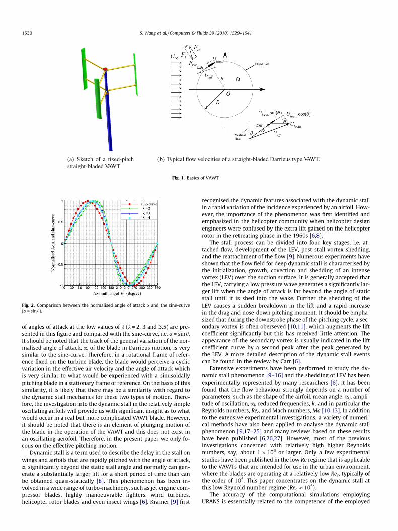
(a) Sketch of a fixed-pitchstraight-bladed VAWT.

(b) Typical flow velocities of a straight-bladed Darrieus type VAWT.

Fig. 1. Basics of VAWT.

Fig. 2. Comparison between the normalised angle of attack a and the sine-curve(a = sinh).

1530 S. Wang et al. / Computers & Fluids 39 (2010) 1529–1541

of angles of attack at the low values of k (k = 2, 3 and 3.5) are pre-sented in this figure and compared with the sine-curve, i.e. a = sinh.It should be noted that the track of the general variation of the nor-malised angle of attack, a, of the blade in Darrieus motion, is verysimilar to the sine-curve. Therefore, in a rotational frame of refer-ence fixed on the turbine blade, the blade would perceive a cyclicvariation in the effective air velocity and the angle of attack whichis very similar to what would be experienced with a sinusoidallypitching blade in a stationary frame of reference. On the basis of thissimilarity, it is likely that there may be a similarity with regard tothe dynamic stall mechanics for these two types of motion. There-fore, the investigation into the dynamic stall in the relatively simpleoscillating airfoils will provide us with significant insight as to whatwould occur in a real but more complicated VAWT blade. However,it should be noted that there is an element of plunging motion ofthe blade in the operation of the VAWT and this does not exist inan oscillating aerofoil. Therefore, in the present paper we only fo-cous on the effective pitching motion.

Dynamic stall is a term used to describe the delay in the stall onwings and airfoils that are rapidly pitched with the angle of attack,a, significantly beyond the static stall angle and normally can gen-erate a substantially larger lift for a short period of time than canbe obtained quasi-statically [8]. This phenomenon has been in-volved in a wide range of turbo-machinery, such as jet engine com-pressor blades, highly manoeuvrable fighters, wind turbines,helicopter rotor blades and even insect wings [6]. Kramer [9] first

recognised the dynamic features associated with the dynamic stallin a rapid variation of the incidence experienced by an airfoil. How-ever, the importance of the phenomenon was first identified andemphasized in the helicopter community when helicopter designengineers were confused by the extra lift gained on the helicopterrotor in the retreating phase in the 1960s [6,8].

The stall process can be divided into four key stages, i.e. at-tached flow, development of the LEV, post-stall vortex shedding,and the reattachment of the flow [9]. Numerous experiments haveshown that the flow field for deep dynamic stall is characterised bythe initialization, growth, covection and shedding of an intensevortex (LEV) over the suction surface. It is generally accepted thatthe LEV, carrying a low pressure wave generates a significantly lar-ger lift when the angle of attack is far beyond the angle of staticstall until it is shed into the wake. Further the shedding of theLEV causes a sudden breakdown in the lift and a rapid increasein the drag and nose-down pitching moment. It should be empha-sized that during the downstroke phase of the pitching cycle, a sec-ondary vortex is often oberseved [10,11], which augments the liftcoefficient significantly but this has received little attention. Theappearance of the secondary vortex is usually indicated in the liftcoefficient curve by a second peak after the peak generated bythe LEV. A more detailed description of the dynamic stall eventscan be found in the review by Carr [6].

Extensive experiments have been performed to study the dy-namic stall phenomenon [9–16] and the shedding of LEV has beenexperimentally represented by many researchers [6]. It has beenfound that the flow behaviour strongly depends on a number ofparameters, such as the shape of the airfoil, mean angle, a0, ampli-tude of oscillation, al, reduced frequencies, k, and in particular theReynolds numbers, Rec, and Mach numbers, Ma [10,13]. In additionto the extensive experimental investigations, a variety of numeri-cal methods have also been applied to analyse the dynamic stallphenomenon [9,17–25] and many reviews based on these resultshave been published [6,26,27]. However, most of the previousinvestigations concerned with relatively high higher Reynoldsnumbers, say, about 1 � 106 or larger. Only a few experimentalstudies have been published in the low Re regime that is applicableto the VAWTs that are intended for use in the urban environment,where the blades are operating at a relatively low Rec, typically ofthe order of 105. This paper concentrates on the dynamic stall atthis low Reynold number regime (Rec � 105).

The accuracy of the computational simulations employingURANS is essentially related to the competence of the employed

S. Wang et al. / Computers & Fluids 39 (2010) 1529–1541 1531

turbulence model. Many popularly used turbulence models foraerodynamic simulations, such as Baldwin–Lomax, RNG k � e, Spal-art-Allmaras, as well as baseline k �x model, nonlinear eddy-vis-cosity models, etc., have been evaluated for the ability ofsimulating this type of complex flow [21,23,24,28]. However,almost all of the models fail to generate results which canconsistently agree well with the experimental data, in particularfor those pitching patterns associated with higer angles of attackand high reduced frequency. The standard k �x model and theSST k �x model (which is a combination of the standard k �xand k � e models) have been reported to perform well in flowswith large separation regions and severe adverse pressure gradi-ents. The description of these turbulence models are detailed in[29,30]. To the best of our knowledge, there is still only a fewnumerical investigations that employ these models to simulatethe dynamic stall phenomenon associated with low Reynolds num-ber (around 105) turbulence flow regime. The only papers that wehave located that involve low Reynolds number flow are the inves-tigation of Spentzos et al. [24] and the recently published paper byMartinat et al. [31]. Therefore, the objective of this paper is toassess the ability of the standard k �x model and the SST k �xmodel to correctly simulate dynamic stall in the low Reynoldsnumber regime which is found in VAWTs and make a contributiontowards a better understanding of the flow physics of dynamic stallin order to assist in the design optimizations of VAWTs intendedfor the built and urban environment in the future.

2. CFD simulations

2.1. The cases investigated

In this paper, we numerically investigate two experimentalcases associated with deep dynamic stall with different bladepitching patterns. Case I is the experimental investigation of Wern-ert et al. [9] and Case II is from the study of Lee and Gerontakos[16]. In both cases, the blade executes an oscillatory motion arounda fixed pivot with the angle of attack following the sinusoidal modegiven by the function a = a0 + al sin(xt), but with different mean

Fig. 3. Illustration of blade pitching motion.

Table 1Validation case specifications for dynamic stall.

Conditions Oscillating pattern

Case I: Wernet et al. [9]Rec = 3.73 � 105, Ma = 0.1 a = 15� + 10�sin(xt)U1 = 28 m/s x = 41.89 rad/s, k = 0.1NACA0012 with c = 0.20 m pitching axis locationspan = 0.56 m the leading edge = 0.25

Case II: Lee and Gerontakos [16]Rec = 1.35 � 105, Ma = 0.04 a = 10� + 15�sin(xt)U1 = 14 m/s x = 18.67 rad/s, k = 0.1NACA0012 with c = 0.15 m pitching axis locationspan = 0.375 m the leading edge = 0.25

angles of attack a0, pitching magnitude al and reduced frequencyk, see Fig. 3. Table 1 gives a summary of the operating conditionsemployed in the two experiments.

With regard to the reasons for the choice of the two cases, firstof all, the range of the Reynolds number is the basic requirementfor the purpose of the present research which excludes a large por-tion of the experimental work. In particular, the Case I is selectedprimarily due to the availability of the near-wall profiles of velocitymagnitude at the airfoil suction side as these are very useful in thevalidation of the numerical results. In the literature, many investi-gations into the aerodynamics of the pitching blade motion havereported information on the integral aerodynamic loads and mo-ments on the airfoils but very few present the velocity fieldsaround the airfoil. Unfortunately, experimental data on the instan-taneous aerodynamic load loops during a complete pitching cyclethat are also essential in order to assess the computational workis not available in this investigation. Therefore, to complementCases I and II which contains such experimental data is chosen.In addition, the coverage of both positive and negative angles of at-tack in Case II is what occurs in the real Darrieus type motion.

2.1.1. Case I: Wernert et al. [9]The airfoil in this case executes the sinusoidal pitching motion

a = 15� + 10�sin(41.89t) with a reduced frequency of k = 0.15. Thefree stream velocity is 28 m/s, resulting in a Reynolds numberRec of 3.73 � 105, based on the chord length. The experimentalinvestigation was conducted in a low-speed wind tunnel whichhas an open, rectangular test section of 70 cm in width, 80 cm inlength and 90 cm in height. The blade was mounted betweentwo circular end plates with a diameter of 40 cm to ensure atwo-dimensional flow in the vertical centre plane of the test sec-tion. The dynamic stall process on a pitching NACA0012 airfoilwith a chord length of 0.2 m was experimentally investigatedemploying particle image velocimetry (PIV) and Laser-SheetVisulisations (LSV).

2.1.2. Case II: Lee and Gerontakos [16]In this case, the blade oscillates with the sinusoidal mode:

a = 10� + 15�sin(18.67t) with a reduced frequency k = 0.10. Thefree stream velocity is U1 = 14 m/s, the turbulence intensity isabout 0.08%, and the Reynolds number is Rec = 1.35 � 105. Theexperiment was conducted in a low-speed, suction-type wind tun-nel with a wall-bounded test section of 120 cm in width, 270 cm inlength and 90 cm in height. The blade was fitted with two endplates with 30 cm in diameter to diminish the end effects. The gapsbetween the oscillatory airfoil and the stationary end plates werekept within 1mm to minimize the leakage of the blade-tip flow.

The transient behaviour of the blade surface unsteady boundarylayer and the characteristics of the dynamic stall events associatedwith an oscillating NACA0012 airfoil were studied using multiplehot-film sensor arrays. In addition, surface pressure measurements

Measurement technique

PIV and LSV,5 low-speed wind tunnel withfrom an open, rectangular testc section of 70 cm � 80 cm � 90 cm

Hot film, hot wire, SV, surface pressure0 measurement, low-speed wind tunnelfrom with a wall-bounded test section ofc 120 cm � 270 cm � 90 cm

1532 S. Wang et al. / Computers & Fluids 39 (2010) 1529–1541

and smoke flow visulisations were performed as a supplement tothe hot-film data. The aerodynamic forces and moments can be de-rived from the blade surface pressure measurements.

2.2. Numerical technique

It is well known that there are three main forms of turbulencesimulation methods, i.e. Direct Numerical Simulation (DNS), LargeEddy Simulation (LES) and Reynolds-Averaged Navier–Stokes(RANS). DNS, despite being the most advanced computational ap-proach, in which all the space and time scales are resolved, de-mands huge computing resources and is still too prohibitive tobe used in the unsteady complicated simulation involved in therange of Reynolds numbers studied in this paper. Although thecomputational power has been at a very high level, it is still verycomputationally expensive to employ LES to numerically investi-gate the complex unsteady dynamic stall phenomenon since 3Dsimulations should be performed due to the 3D nature of the ed-dies. For the present, URANS appears to be the most suitable ap-proach to conduct the dynamic stall flow simulations with anacceptable computational cost and, at least, reasonable accuracy.Therefore, in the present study, the URANS method is employed.

Although the dynamic stall flow studied here is inherently a 3Dphenomenon, measurements have been taken to ensure a 2D flowin the mid-span plane, where the experimental data were ob-tained, in both the two cases investigated. In Case I, the 2D flowin the plane was verified by flow visulisation experiments whilein Case II, the 2D uniformity of the flow over the airfoil was foundto be within 4% of the free stream value, as checked by a hot-wireprobe. Thus, in the present simulations, 2D geometrical configura-tions are employed to model the experimental investigations and a2D incompressible unsteady CFD solver, based on the finite volumemethod in the commercial software package Fluent, is employed tosolve the full URANS governing equations. Due to the incompress-ibility of the flow studied, the pressure-based solver, which em-ploys an algorithm which belongs to the so-called ‘‘projectionmethod” and is traditionally implemented to solve low-speedincompressible flows, is chosen. All the governing equations forthe solution variables, which are decoupled from each other, aresolved sequentially and the SIMPLE algorithm is applied as thepressure-velocity coupling algorithm. With respect to the discreti-zation of the convection terms in the transport equations for thevelocity and the turbulence quantities, second-order upwindschemes are utilised. In order to accelerate the rate of convergenceof the solution, the algebraic multigrid scheme (AMG) with a V-cy-cle type for the pressure and a flexible type for the momentumequations is applied. A detailed description of these methods canbe found in [32]. The calculations have been carried out usingthe standard k �x model, assuming that the flow of the airfoil isfully turbulent and the SST k �x model with prediction of the lam-inar-to-turbulence transitional process. The modelling of transitionis realised by damping the turbulent viscosity lt which is com-puted as follows with the coefficient a* [33]:

lt ¼qkx

1

max 1a� ;

SF2a1x

h i ; where a� ¼ 0:024þ Ret=61þ Ret=6

; Ret ¼qklx

:

All the numerical simulations are performed at the same conditionsas those of the experimental settings to simulate the flow field atthe mid cross-section of the experimental setup.

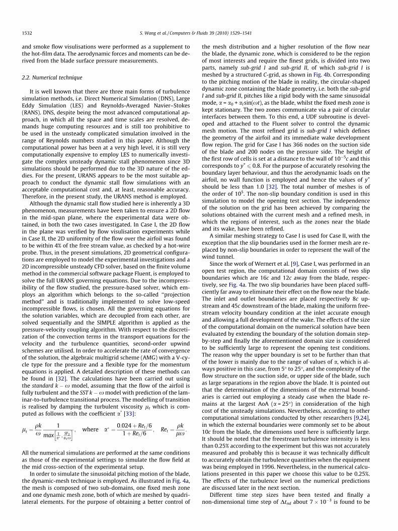
In order to simulate the sinusoidal pitching motion of the blade,the dynamic-mesh technique is employed. As illustrated in Fig. 4a,the mesh is composed of two sub-domains, one fixed mesh zoneand one dynamic mesh zone, both of which are meshed by quadri-lateral elements. For the purpose of obtaining a better control of

the mesh distribution and a higher resolution of the flow nearthe blade, the dynamic zone, which is considered to be the regionof most interests and require the finest grids, is divided into twoparts, namely sub-grid I and sub-grid II, of which sub-grid I ismeshed by a structured C-grid, as shown in Fig. 4b. Correspondingto the pitching motion of the blade in reality, the circular-shapeddynamic zone containing the blade geometry, i.e. both the sub-gridI and sub-grid II, pitches like a rigid body with the same sinusoidalmode, a = a0 + al sin(xt), as the blade, whilst the fixed mesh zone iskept stationary. The two zones communicate via a pair of circularinterfaces between them. To this end, a UDF subroutine is devel-oped and attached to the Fluent solver to control the dynamicmesh motion. The most refined grid is sub-grid I which definesthe geometry of the airfoil and its immediate wake developmentflow region. The grid for Case I has 366 nodes on the suction sideof the blade and 200 nodes on the pressure side. The height ofthe first row of cells is set at a distance to the wall of 10�5c and thiscorresponds to y+

6 0.8. For the purpose of accurately resolving theboundary layer behaviour, and thus the aerodynamic loads on theairfoil, no wall function is employed and hence the values of y+

should be less than 1.0 [32]. The total number of meshes is ofthe order of 105. The non-slip boundary condition is used in thissimulation to model the opening test section. The independenceof the solution on the grid has been achieved by comparing thesolutions obtained with the current mesh and a refined mesh, inwhich the regions of interest, such as the zones near the bladeand its wake, have been refined.

A similar meshing strategy to Case I is used for Case II, with theexception that the slip boundaries used in the former mesh are re-placed by non-slip boundaries in order to represent the wall of thewind tunnel.

Since the work of Wernert et al. [9], Case I, was performed in anopen test region, the computational domain consists of two slipboundaries which are 16c and 12c away from the blade, respec-tively, see Fig. 4a. The two slip boundaries have been placed suffi-ciently far away to eliminate their effect on the flow near the blade.The inlet and outlet boundaries are placed respectively 8c up-stream and 45c downstream of the blade, making the uniform free-stream velocity boundary condition at the inlet accurate enoughand allowing a full development of the wake. The effects of the sizeof the computational domain on the numerical solution have beenevaluated by extending the boundary of the solution domain step-by-step and finally the aforementioned domain size is consideredto be sufficiently large to represent the opening test conditions.The reason why the upper boundary is set to be further than thatof the lower is mainly due to the range of values of a, which is al-ways positive in this case, from 5� to 25�, and the complexity of theflow structure on the suction side, or upper side of the blade, suchas large separations in the region above the blade. It is pointed outthat the determination of the dimensions of the external bound-aries is carried out employing a steady case when the blade re-mains at the largest AoA (a = 25�) in consideration of the highcost of the unsteady simulations. Nevertheless, according to othercomputational simulations conducted by other researchers [9,24],in which the external boundaries were commonly set to be about10c from the blade, the dimensions used here is sufficiently large.It should be noted that the freestream turbulence intensity is lessthan 0.25% according to the experiment but this was not accuratelymeasured and probably this is because it was technically difficultto accurately obtain the turbulence quantities when the equipmentwas being employed in 1996. Nevertheless, in the numerical calcu-lations presented in this paper we choose this value to be 0.25%.The effects of the turbulence level on the numerical predictionsare discussed later in the next section.

Different time step sizes have been tested and finally anon-dimensional time step of Dtnd about 7 � 10�3 is found to be

(a) Diagram of the model geometry, boundary conditionsand mesh structure.

(b) Diagram of the sub-grid structure.

Fig. 4. Computational setup.

Table 2Residual convergence criterion for all the solution quantities.

Variable Continuityequation

ux uy k x

Convergence criterion 610�5610�7

6 10�7610�9

610�8

S. Wang et al. / Computers & Fluids 39 (2010) 1529–1541 1533

sufficiently small for the time-independent solution to be obtainedfor the two cases studied and this has been achieved by checkingthe time history of Cl, Cd and Cm. The calculations start from an ini-tial flow field obtained from a well converged steady state compu-tation where the airfoil is positioned at the mean angle of attackand, in order to remove the influence of the initial flow field, a suf-ficient number of cycles of the airfoil pitching motion have beencalculated until a periodic solution is achieved for Case I. However,for Case II, due to the severe fluctuations of the computed forces,only a quasi-periodic solution is obtained. Regarding the conver-gence criteria, the residual for the continuity equation is set tobe less than 10�5. See Table 2 for the details of all the computedquantities. In order to confirm that the criteria is sufficient to en-sure the convergence of solutions within one time step, the resid-ual for the continuity equation is reset to 10�4. We found that

almost no differences can be found between the two set of solu-tions and this indicates that the current convergence criteria is suf-ficient to produce converged solutions within one time step in thepresent study.

3. Results and discussions

3.1. Simulations of the Wernert et al. [9] test case, Case I

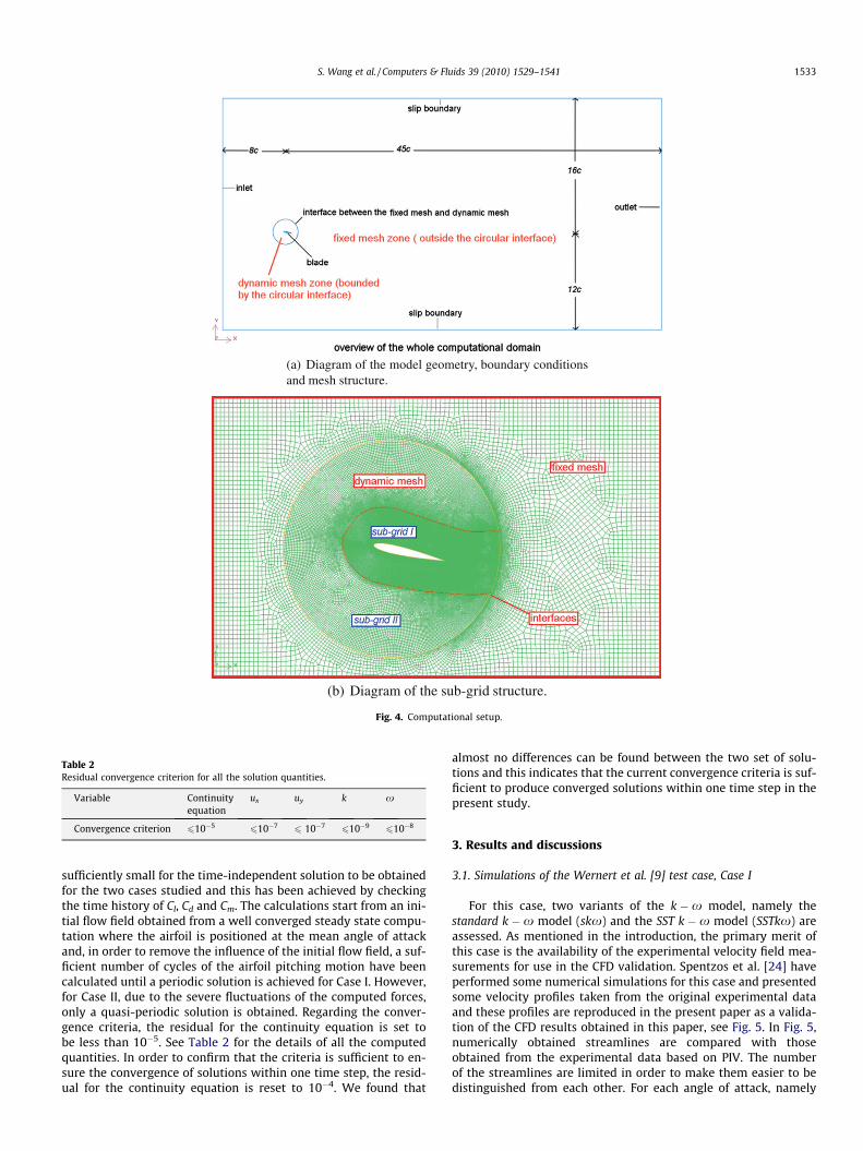
For this case, two variants of the k �x model, namely thestandard k �x model (skx) and the SST k �x model (SSTkx) areassessed. As mentioned in the introduction, the primary merit ofthis case is the availability of the experimental velocity field mea-surements for use in the CFD validation. Spentzos et al. [24] haveperformed some numerical simulations for this case and presentedsome velocity profiles taken from the original experimental dataand these profiles are reproduced in the present paper as a valida-tion of the CFD results obtained in this paper, see Fig. 5. In Fig. 5,numerically obtained streamlines are compared with thoseobtained from the experimental data based on PIV. The numberof the streamlines are limited in order to make them easier to bedistinguished from each other. For each angle of attack, namely

(b) Angle of attack α = 24 , upstroke.º

(a) Angle of attack α = 22 , upstroke.º

Fig. 5. Comparison between the numerical results and the experimental data of Wernert et al. [9], Case I.

1534 S. Wang et al. / Computers & Fluids 39 (2010) 1529–1541

a = 22� and 24�, there are three plots, presenting the variation ofthe non-dimensional velocity magnitude u/U1 with the non-dimensional distance from the blade d/c, corresponding to threechordwise locations, x/c = 0.25, 0.5, 0.75. It should be noted inFig. 5 that the magnitude of the fluid velocity is assigned a sign, po-sitive meaning the flow goes from the leading edge to the trailingedge and negative meaning the reverse (This assignment is notdone for the results of the SSTkx model at a = 24� since this willcause significant intermittence of the curves).

It can be easily seen from the streamlines that the LEV has beencaptured by both the skx model and the SSTkx model, whereas the

position and the size of the LEVs obtained by the two models arequite different. In general, the skx model generates a more stableflow structure than does the SSTkx model and it smears out thesmall circulations in the near-wall region at a = 24�. In contrastto the skx model, the SSTkx model presents a more complex flowstructure, especially at a high angle of attack where the twosecondary counter-rotating vortices are obtained which appearsto be more realistic, since it is also mentioned that small-scalevortices can be recognised on the PIV pictures, even with the largedynamic stall vortex by Wernert et al. [9]. This conclusion has alsobeen obtained by other researchers [8,23,34]. The computed

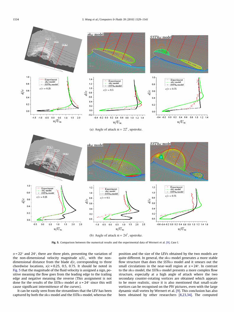
Fig. 6. History of the sectional lift coefficient within six pitching cycles for Case II.

S. Wang et al. / Computers & Fluids 39 (2010) 1529–1541 1535

chordwise spatial extension of about 75% c using the SSTkx modelis in good agreement with the experimental data. It can be seenthat the chordwise dimensions of the vortices in the SSTkx modelresults are much more constrained than those obtained in the skxmodel, whilst their thickness is much bigger. This may be becausethe skx model is more dissipative in terms of the eddy energy andfails to predict the severe adverse pressure gradient, making thepredicted LEV span a larger portion of the blade. Also a similar con-clusion has been drawn by Martinat et al. [31]. Another reason forthis may lie in the assumption of fully turbulent flow on the airfoilin the theory of the skx model, whereas the transition in theboundary layer from laminar-to-turbulence at the leading edgeof the blade is predicted in the SSTkx model. The use of fullturbulence models can limit the occurrence of the laminar separa-tion at the leading edge of the airfoil, leading to an inaccurateturbulent flow development, as well as the prediction of thedevelopment of the LEV. A comparison of the streamlines obtainedfrom the PIV data shows that the SSTkx model clearly performsbetter than the skx model, which over-predicts the chordwisespan of the LEV.

Regarding the comparison between the velocity profiles at theaforementioned three chordwise locations, the results agree betterat low angles of attack than at high angles of attack for both mod-els. At high angles of attack the airfoil turns into deep stall and theflow becomes fully separated. For separation flows, the 3D effectsshould be more significant than those without separations at smal-ler angles of attack, see [34]. This is where both models fail tomatch the experimental data. At a = 22�, the velocity profile ob-tained employing the SSTkx model at x = 0.25c agrees remarkablywell with the experimental data while the skx model fails to cap-ture the maximum velocity and the sharp structure, see Fig. 5a.Compared with the streamlines at this postion, this indicates thatthe scale and position of the LEV are predicted reasonably wellby the SSTkx model at lower values of a. At the position of 0.5c,it can be seen that the skx model still predicts a recirculation inthe boundary layer while the LEV has already ended by this pointfrom the results gleaned from the SSTkx model. At x = 0.75c, theresults obtained from the SSTkx model agree well with the exper-imental data in regions further away from the blade and close tothe boundary layer. However, the transition of the velocity profilebetween these two regions appears to be not accurate enough incontrast to the experimental curve. The LEV predicted by the skxmodel extends even to this chordwise location and clearly thisshould be an overshoot in the span of the LEV in comparison withthe validation data. At high angles of attack, say a = 24�, althoughthe skx model appears to present a better trend in comparisonwith the experimental data, the flow structure differs significantlyfrom the experimental results according to the streamline patterns.Thus, the better agreement with the validation velocity profiles forthe skx model may be considered as fortuitous. Further, it shouldbe noted that both of the two numerical models overestimate themagnitude of the velocities in the region further away from thewall where d/c P 0.4.

It should be noted that despite many efforts to eliminate the 3Deffects on the testing surface in the experiment, there are still some3D effects according to the experimental work of Raffel et al. [11],which is based on the same experiment of Wernert et al. [9] if notexactly the same. In addition, because of the limitations in the laserpulse rate and framing speed of the photo camera used in thisexperiment, it was impossible to record the flow field at all the dif-ferent angles of attack of the blade within one pitching cycle but insuccessive periods. What is more, the experimental research wasperformed twelve years ago, and because of the strong unsteadycharacteristics of the flow field, the accuracy of the data is stillan open question. Potentially, these may be reasons for the dis-crepancies between the numerical and experimental data.

3.2. Simulations of the Lee and Gerontakos [16] test case, Case II

In general, for Case I, the SSTkx model produces more accuratepredictions than does the skx model and hence this turbulencemodel is employed in Case II.

Under the operating conditions in this case, a large cycle-to-cy-cle difference of the solutions at high angles of attack during boththe upstroke and downstroke pitching phases is observed. Fig. 6shows the history of the sectional lift coefficient, Cl, in six pitchingcycles starting from the mean angle of attack, i.e. a = 10�. This kindof aperiodic or quasi-periodic flow phenomenon is also observed inthe experiments [9–11].

The numerically computed coefficients of the aerodynamicforces obtained from a pitching cycle are presented in Fig. 7 andcompared with the experimental data. It can be seen that withinthe range of low and medium angles of attack, i.e. �5� 6 a 6 20�,the CFD results for the coefficients of aerodynamic forces agreewell with the experimental data, fluctuating around the measureddata. This is an indication that the SSTkx model performs well atthese values of angle of attack. However, similar to the results ob-tained for the case of Wernert et al. [9], Case I, at the high angles ofattack, 20� 6 a 6 25�, where deep stall may be expected, thenumerical results have a much larger difference from the experi-mental data.

From Fig. 7a, it is seen clearly that the position of the intersec-tion point 1 between the upstroke and downstroke paths of thesectional lift coefficient at a � 0� is well captured by point 10 aswell as the intersection 1 of the sectional drag coefficient inFig. 7b. However, the absolute values are not exactly the same. Fur-ther, the capture of the other intersection, point 2 in Fig. 7b, is notas accurately predicted, and the numerical curve shows a stronginstability at high angles of attack.

The reduction in the lift coefficient for 20� < a < 25� correspondsto the shedding of the LEV, while there is a sudden increase in thelift coefficient near the maximum angle of attack during the down-stroke phase and this is an indication of the generation of the sec-ondary vortex. Firstly, it appears that there is a phase shift betweenthe numerical and experimental results since the secondary vortexappears to occur at about a = 22� in the downstroke motion. This isdiscussed by McCroskey et al. [12], namely both the strength andphase of the dynamic forces depend upon the reduced frequencyk. As shown in Fig. 9, which is adapted from that presented byMcCroskey et al. [12], as k increases, the phase of the normal forcecurve shifts to the right, or rather it causes a delay in the phase ofthe dynamic stall. At k = 0.05, both the shedding of the LEV and thegeneration of the secondary vortex occurs before the maximumangle of attack when the blade is still in the upstroke phase. Atk = 0.15, the occurrence of the secondary vortex has already been

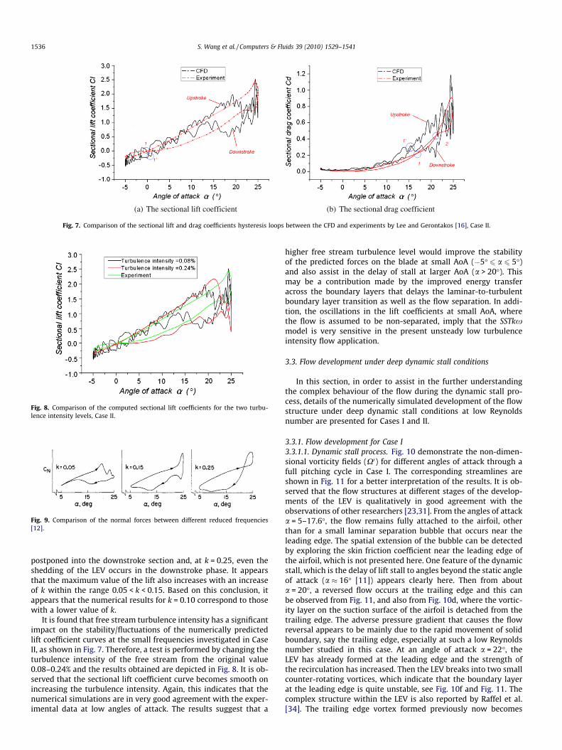
Fig. 8. Comparison of the computed sectional lift coefficients for the two turbu-lence intensity levels, Case II.

Fig. 9. Comparison of the normal forces between different reduced frequencies[12].

(a) The sectional lift coefficient (b) The sectional drag coefficient

Fig. 7. Comparison of the sectional lift and drag coefficients hysteresis loops between the CFD and experiments by Lee and Gerontakos [16], Case II.

1536 S. Wang et al. / Computers & Fluids 39 (2010) 1529–1541

postponed into the downstroke section and, at k = 0.25, even theshedding of the LEV occurs in the downstroke phase. It appearsthat the maximum value of the lift also increases with an increaseof k within the range 0.05 < k < 0.15. Based on this conclusion, itappears that the numerical results for k = 0.10 correspond to thosewith a lower value of k.

It is found that free stream turbulence intensity has a significantimpact on the stability/fluctuations of the numerically predictedlift coefficient curves at the small frequencies investigated in CaseII, as shown in Fig. 7. Therefore, a test is performed by changing theturbulence intensity of the free stream from the original value0.08–0.24% and the results obtained are depicted in Fig. 8. It is ob-served that the sectional lift coefficient curve becomes smooth onincreasing the turbulence intensity. Again, this indicates that thenumerical simulations are in very good agreement with the exper-imental data at low angles of attack. The results suggest that a

higher free stream turbulence level would improve the stabilityof the predicted forces on the blade at small AoA (�5� 6 a 6 5�)and also assist in the delay of stall at larger AoA (a > 20�). Thismay be a contribution made by the improved energy transferacross the boundary layers that delays the laminar-to-turbulentboundary layer transition as well as the flow separation. In addi-tion, the oscillations in the lift coefficients at small AoA, wherethe flow is assumed to be non-separated, imply that the SSTkxmodel is very sensitive in the present unsteady low turbulenceintensity flow application.

3.3. Flow development under deep dynamic stall conditions

In this section, in order to assist in the further understandingthe complex behaviour of the flow during the dynamic stall pro-cess, details of the numerically simulated development of the flowstructure under deep dynamic stall conditions at low Reynoldsnumber are presented for Cases I and II.

3.3.1. Flow development for Case I3.3.1.1. Dynamic stall process. Fig. 10 demonstrate the non-dimen-sional vorticity fields (X0) for different angles of attack through afull pitching cycle in Case I. The corresponding streamlines areshown in Fig. 11 for a better interpretation of the results. It is ob-served that the flow structures at different stages of the develop-ments of the LEV is qualitatively in good agreement with theobservations of other researchers [23,31]. From the angles of attacka = 5–17.6�, the flow remains fully attached to the airfoil, otherthan for a small laminar separation bubble that occurs near theleading edge. The spatial extension of the bubble can be detectedby exploring the skin friction coefficient near the leading edge ofthe airfoil, which is not presented here. One feature of the dynamicstall, which is the delay of lift stall to angles beyond the static angleof attack (a � 16� [11]) appears clearly here. Then from abouta = 20�, a reversed flow occurs at the trailing edge and this canbe observed from Fig. 11, and also from Fig. 10d, where the vortic-ity layer on the suction surface of the airfoil is detached from thetrailing edge. The adverse pressure gradient that causes the flowreversal appears to be mainly due to the rapid movement of solidboundary, say the trailing edge, especially at such a low Reynoldsnumber studied in this case. At an angle of attack a = 22�, theLEV has already formed at the leading edge and the strength ofthe recirculation has increased. Then the LEV breaks into two smallcounter-rotating vortices, which indicate that the boundary layerat the leading edge is quite unstable, see Fig. 10f and Fig. 11. Thecomplex structure within the LEV is also reported by Raffel et al.[34]. The trailing edge vortex formed previously now becomes

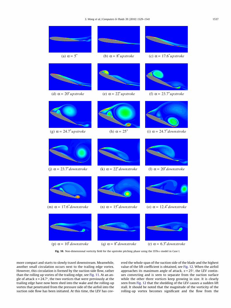
(r) α = 6.3 downstrokeº(q) α = 8 downstrokeº(p) α = 10 downstrokeº

(m) α = 17.6 downstrokeº (n) α = 15 downstrokeº (o) α = 12.4 downstrokeº

(l) α = 20 downstrokeº(k) α = 22 downstrokeº(j) α = 23.7 downstrokeº

(g) α = 24.7 upstrokeº (h) α = 25º (i) α = 24.7 downstrokeº

(d) α = 20 upstrokeº (e) α = 22 upstrokeº (f) α = 23.7 upstrokeº

(c) α = 17.6 upstrokeº(b) α = 8 upstrokeº(a) α = 5º

Fig. 10. Non-dimensional vorticity field for the upstroke pitching phase using the SSTkx model in Case I.

S. Wang et al. / Computers & Fluids 39 (2010) 1529–1541 1537

more compact and starts to slowly travel downstream. Meanwhile,another small circulation occurs next to the trailing edge vortex.However, this circulation is formed by the suction side flow, ratherthan the rolling up vortex of the trailing edge, see Fig. 11. At an an-gle of attack a = 24.7�, the two vortices that were previously at thetrailing edge have now been shed into the wake and the rolling-upvortex that penetrated from the pressure side of the airfoil into thesuction side flow has been initiated. At this time, the LEV has cov-

ered the whole span of the suction side of the blade and the highestvalue of the lift coefficient is obtained, see Fig. 12. When the airfoilapproaches its maximum angle of attack, a = 25�, the LEV contin-ues convecting and is seen to separate from the suction surfacewhile the other three vortices keep growing in size. It is clearlyseen from Fig. 12 that the shedding of the LEV causes a sudden liftstall. It should be noted that the magnitude of the vorticity of therolling-up vortex becomes significant and the flow from the

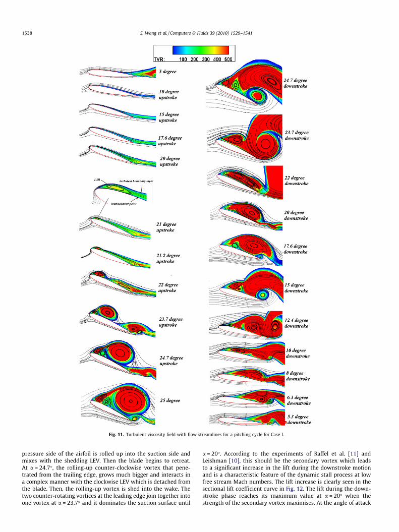
Fig. 11. Turbulent viscosity field with flow streamlines for a pitching cycle for Case I.

1538 S. Wang et al. / Computers & Fluids 39 (2010) 1529–1541

pressure side of the airfoil is rolled up into the suction side andmixes with the shedding LEV. Then the blade begins to retreat.At a = 24.7�, the rolling-up counter-clockwise vortex that pene-trated from the trailing edge, grows much bigger and interacts ina complex manner with the clockwise LEV which is detached fromthe blade. Then, the rolling-up vortex is shed into the wake. Thetwo counter-rotating vortices at the leading edge join together intoone vortex at a = 23.7� and it dominates the suction surface until

a = 20�. According to the experiments of Raffel et al. [11] andLeishman [10], this should be the secondary vortex which leadsto a significant increase in the lift during the downstroke motionand is a characteristic feature of the dynamic stall process at lowfree stream Mach numbers. The lift increase is clearly seen in thesectional lift coefficient curve in Fig. 12. The lift during the down-stroke phase reaches its maximum value at a = 20� when thestrength of the secondary vortex maximises. At the angle of attack

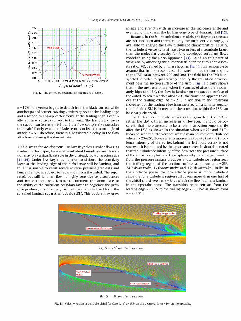
Fig. 12. The computed sectional lift coefficient of Case I.

S. Wang et al. / Computers & Fluids 39 (2010) 1529–1541 1539

a = 17.6�, the vortex begins to detach from the blade surface whileanother pair of couner-rotating vortices appear at the leading edgeand a second rolling-up vortex forms at the trailing edge. Eventu-ally, all these vortices convect to the wake. The last vortex leavesthe suction surface at a = 6.3�, and the flow completely reattachesto the airfoil only when the blade returns to its minimum angle ofattack, a = 5�. Therefore, there is a considerable delay in the flowattachment during the downstroke.

3.3.1.2. Transition development. For low Reynolds number flows, asstudied in this paper, laminar-to-turbulent boundary-layer transi-tion may play a significant role in the unsteady flow characteristics[34–36]. Under low Reynolds number conditions, the boundarylayer at the leading edge of the airfoil may still be laminar, andthus it is unable to resist severe adverse pressure gradients andhence the flow is subject to separation from the airfoil. The sepa-rated, but still laminar, flow is highly sensitive to disturbancesand hence experiences laminar-to-turbulent transition. Due tothe ability of the turbulent boundary layer to negotiate the pres-sure gradient, the flow may reattach to the airfoil and form theso-called laminar separation bubble (LSB). This bubble may grow

(b) α = 10 on thº

(a) α = 5.5 on thº

Fig. 13. Velocity vectors around the airfoil for Case II. (a)

in size and strength with an increase in the incidence angle andeventually this causes the leading-edge type of dynamic stall [12].

Because, in the k �x turbulence models, the Reynolds stressesare not modelled and therefore only the turbulent viscosity lt isavailable to analyse the flow turbulence characteristics. Usually,the turbulent viscosity is at least two orders of magnitude largerthan the molecular viscosity for fully developed turbulent flowsmodelled using the RANS approach [33]. Based on this point ofview, and by observing the numerical field for the turbulent viscos-ity ratio,TVR, defined by lt/l, as shown in Fig. 11, it is reasonable toassume that in the present case the transition region correspondsto the TVR value between 200 and 300. The field for the TVR is in-spected in order to qualitatively identify the transition develop-ment near the suction surface of the airfoil. Fig. 11 clearly showsthat in the upstroke phase, when the angles of attack are moder-ately high (a < 18�), the flow is laminar on the suction surface ofthe airfoil. When a reaches about 20�, the transition appears to oc-cur at the trailing edge. At a = 21�, in addition to the upstreammovement of the trailing edge transition region, a laminar separa-tion bubble (LSB) is formed and the transition within the LSB canbe clearly observed.

The turbulence intensity grows as the growth of the LSB orrather the LEV with an increase in a. However, it should be ob-served that there appears to be a relaminarization zone shortlyafter the LSV, as shown in the situation when a = 22� and 23.7�.It can be seen that the vortices are the main sources of turbulencewhen a = 23–25�. However, it is interesting to note that the turbu-lence intensity of the vortex behind the left-most vortex is notstrong as it is protected by the upstream vortex. It should be notedthat the turbulence intensity of the flow near the pressure surfaceof the airfoil is very low and this explains why the rolling-up vortexfrom the pressure surface produces a low turbulence region nearthe trailing region of the suction surface, as shown at a = 25�,24.7�downstroke, 17.6�downstroke and 15� downstroke. Unlike inthe upstroke phase, the downstroke phase is more turbulentsince the fully turbulent region still covers more than one half ofthe airfoil chord, even at a = 8� at which the flow is almost laminarin the upstroke phase. The transition point retreats from theleading edge x � 0.2c to the trailing edge x � 0.75c, as shown froma = 8–5.3�.

e upstroke .

e upstroke .

a = 5.5� on the upstroke, (b) a = 10� on the upstroke.

1540 S. Wang et al. / Computers & Fluids 39 (2010) 1529–1541

3.3.2. Flow development for Case IIOne feature of the flow development of Case II is the rear-to-

front progression of the trailing edge flow reversal before theoccurrence of the dynamic stall, which is observed in the experi-ment [16]. Further McCroskey et al. [12] also reported investiga-tions of the dynamic stall associated with this kind of flowbehaviour. Fig. 13a shows the computed thin flow reversal layernear the trailing edge on the suction side, which extends to about0.5c from the trailing edge at a = 5.5�. This reversal gradually prop-agates towards the leading edge as the AoA increases and reachesabout 0.1c from the leading edge at a = 10� on the upstroke, asshown in Fig. 13. It should be noted that the thin layer of reversedflow near the suction side is significantly unstable and easilybreaks down into several small-scale vortices which can be seenin Fig. 13. As in the LEV, these small vortices also carry pressurewaves, despite the strength being much smaller than the LEV. Thisappears to be responsible for the oscillations of the aerodynamicloads shown in Fig. 7.

Another characteristic of the stall process observed in Case II isthat the stall is trigged by a turbulent separation at a short distancedownstream of the leading edge bubble, rather than by the burst ofthe bubble. This feature is also well captured by the simulations,since it can be clearly seen from the computed flow field that theleading edge bubble maintains its existence to a very high angleof attack. However it appears from the numerical data that theleading edge bubble is induced to shed vortices from time to time.The effect of the continuous shedding is similar to the turbulentbreakdown as discussed by Lee and Gerontakos [16]. However,the predicted onset of the lift stall is earlier than that observedin the experiments which indicates that the shedding of the LEVis not accurately simulated.

In this section, the flow development events have been dis-cussed and the computational results qualitatively capture wellthe features of the dynamic stall process, such as the formation,convection and shedding of the LEV as well as the secondary vor-tex, and these predictions can provide detailed information onthe flow development.

4. Conclusions

In this study, two URANS models, namely the standard k �xmodel and the SST k �x model with transition, have been em-ployed to simulate the fluid flow around two sinusoidally pitchingNACA0012 airfoils, in the context of the low Reynolds number re-gime, Re � 105. The standard k �x model appears too dissipativeto predict the severe adverse pressure gradient near the suctionside of the blade and this causes an over-prediction of the LEV spanin the chordwise direction and an underestimate of the thicknessof the LEV. The SST k �x model presents an improvement overthe standard k �x model and can predict the experimental datawith reasonable accuracy, other than at very high angles of attackwhere the flow is fully detached and the 3D effect is expected to bemore significant. The characteristics of dynamic stall, such as theLEV-dominated flow structure, the aerodynamic load hysteresisloops, and the secondary vortex in the downstroke phase, is wellcaptured by the SST k �x model. In addition, a fairly reasonabledevelopment of the flow transition before and during the dynamicstall can be numerically obtained. In order to obtain a very detailedunderstanding of the details of the dynamic stall phenomenon, thecapability of other more advanced CFD methods, such as LES orDES, needs to be investigated. In particular for the investigationof the blade/wake interactions in the core of VAWTs, detailedand accurate simulations of the vortex formation and shedding inboth low and high AoA in a transient state needs to be investigated.However, URANS with advanced turbulence models, such as the

SST k �x model as evaluated in this paper, are useful for the fastdesign or research intension for low Reynolds number airfoilsand VAWTs, because they are capable of capturing the experimen-tal data in a significant part of the flow dynamics.

Acknowledgements

The authors would like to acknowledge the financial supportfrom the Chinese Scholarship Council (CSC) for this work. Alsothe authors would like to thank Dr. G. Barakos from The Universityof Liverpool, UK, Professor T. Lee from McGill University, Canada,Mr. Wolfgang Geissler from German Aerospace Centre (DLR) andDr. Philippe Wernert from the French–German Research Instituteof Saint-Louis (ISL), Germany, for their kind support of the researchassociated with this paper.

References

[1] Blackwell B. Vertical-axis wind turbine: how it works. Technical report, SLA-74-0160, Sandia Labs., Albuquerque, N. Mexico (USA); 1974.

[2] Paraschivoiu I. Wind turbine design: with emphasis on Darrieusconcept. Canada: Polytechnic International Press; 2002.

[3] Ferreira C, Bijl H, van Bussel G, van Kuik G. Simulating dynamic stall in a 2DVAWT: modeling strategy, verification and validation with particle imagevelocimetry data. J Phys Conf Ser 2007;75.

[4] Edwards J, Durrani N, Howell R, Qin N. Wind tunnel and numerical study of asmall vertical axis wind turbine. In: 46th AIAA aerospaces sciences meetingand exhibit, Reno, Nevada, vol. 11; 2008.

[5] Simão Ferreira C, van Kuik G, van Bussel G, Scarano F. Visualization by PIV ofdynamic stall on a vertical axis wind turbine. Exp Fluids 2008;46(1):97–108.

[6] Carr L. Progress in analysis and prediction of dynamic stall. J Aircraft1988;25(1):6–17.

[7] Allet A, Halle S, Paraschivoiu I. Numerical simulation of dynamic stall aroundan airfoil in Darrieus motion. J Sol Energy 1999;121:69–76.

[8] Cebeci T, Platzer M, Chen H, Chang K-C, Shao JP. Analysis of low speed unsteadyairfoil flows. Long Beach, California, US and Heidelberg, Germany: HorizonsPublishing; 2005.

[9] Wernert P, Geissler W, Raffel M, Kompenhans J. Experimental and numericalinvestigations of dynamic stall on a pitching airfoil. AIAA J 1996;34(5):982–9.

[10] Leishman J. Dynamic stall experiments on the NACA 23012 aerofoil. Exp Fluids1990;9(1):49–58.

[11] Raffel M, Kompenhans J, Wernert P. Investigation of the unsteady flow velocityfield above an airfoil pitching under deep dynamic stall conditions. Exp Fluids1995;19(2):103–11.

[12] McCroskey W, Carr L, McAlister K. Dynamic stall experiments on oscillatingairfoils. AIAA J 1976;14(1):57–63.

[13] McCroskey W, McAlister K, Carr L, Pucci S. An experimental study of dynamicstall on advanced airfoil sections. Summary of the experiment, vol. 1. NASATechnical Memorandum 84245; 1982.

[14] McAlister K, Pucci S, McCroskey W, Carr L. An experimental study of dynamicstall on advanced airfoil section. Pressure and force data, vol. 2. NASATechnical Memorandum 84245; 1982.

[15] Schreck S, Helin H. Unsteady vortex dynamics and surface pressure topologieson a finite pitching wing. J Aircraft 1994;31(4):899–907.

[16] Lee T, Gerontakos P. Investigation of flow over an oscillating airfoil. J FluidMech 2004;512:313–41.

[17] Wu J, Sankar L, Huff D. Evaluation of three turbulence models for theprediction of steady and unsteady airloads. In: AIAA, the 27th aerospacesciences meeting, Reno, NV; 1989.

[18] Visbal M. Dynamic stall of a constant-rate pitching airfoil. J Aircraft1990;27(5):400–7.

[19] Tuncer I, Wu J, Wang C. Theoretical and numerical studies of oscillatingairfoils. AIAA J 1990;28(9):1615–24.

[20] Ekaterinaris J. Numerical investigation of dynamic stall of an oscillating wing.AIAA J 1995;33(10):1803–8.

[21] Srinivasan G, Ekaterinaris J, McCroskey W, Aeronautics N, Administration S,States U. Evaluation of turbulence models for unsteady flows of an oscillatingairfoil. Comput Fluids 1995;24(7):833–61.

[22] Mellen C, Frohlich J, Rodi W. Lessons from LESFOIL project on large-eddysimulation of flow around an airfoil. AIAA J 2003;41(4):573–81.

[23] Barakos G, Drikakis D. Computational study of unsteady turbulent flowsaround oscillating and ramping aerofoils. Int J Numer Methods Fluids2003;42(2):163–86.

[24] Spentzos A, Barakos G, Badcock K, Richards B, Wernert P, Schreck S, et al.Investigation of three-dimensional dynamic stall using computational fluiddynamics. AIAA J 2005;43(5):1023–33.

[25] Sheng W, Galbraith R, Coton F. A modified dynamic stall model for low machnumbers. J Sol Energy – Trans ASME 2008;130(3):031013.

[26] McCroskey W. The phenomenon of dynamic stall. NASA TM-81264; 1981.[27] McCroskey W. Unsteady airfoils. Annu Rev Fluid Mech 1982;14(1):

285–311.

S. Wang et al. / Computers & Fluids 39 (2010) 1529–1541 1541

[28] Niu Y. Evaluation of renormalization group turbulence models for dynamicstall simulation. AIAA J 1999;37(6):770–1.

[29] Wilcox D. Turbulence modeling for CFD. DCW Industries, La Canada, CA.[30] Menter F. Two-equation eddy-viscosity turbulence models for engineering

applications. AIAA J 1994;32(8):1598–605.[31] Martinat G, Braza M, Hoarau Y, Harran G. Turbulence modelling of the flow

past a pitching NACA0012 airfoil at 105 and 106 Reynolds numbers. J FluidStruct 2008;24(8):1294–303.

[32] Fluent I. Fluent 6. 3 user’s guide. Fluent documentation.

[33] Ansys F. Fluent user’s manual. Software release 6.[34] Raffel M, Favier D, Berton E, Rondot C, Nsimba M, Geissler W. Micro-PIV and

ELDV wind tunnel investigations above a helicopter blade tip. Measur SciTechnol 2006;17:1652–8.

[35] Geissler W, Chandrasekhara M, Platzer M, Carr L. The effect of transitionmodelling on the prediction of compressible deep dynamic stall. In: 7th Asiancongress of fluid mechanics; 1997.

[36] Lissaman P. Low-Reynolds-number airfoils. Annu Rev Fluid Mech 1983;15(1):223–39.