Embed Size (px)
Citation preview
Numerical Methods
for
Inverse Eigenvalue Problems
by
BAI Zheng Jian
A Thesis Submitted in Partial Fulfillment
of the Requirements for the Degree of
Doctor of Philosophy
in
Mathematics
c©The Chinese University of Hong Kong
May 2004
The Chinese University of Hong Kong holds the copyright of this thesis. Any
person(s) intending to use a part or whole of the materials in the thesis in a
proposed publication must seek copyright release from the Dean of the Graduate
School.
Numerical Methods for Inverse Eigenvalue Problems i
Abstract
Abstract of thesis entitled:
Numerical Methods
for
Inverse Eigenvalue Problems
Submitted by BAI Zheng Jian
for the degree of Doctor of Philosophy in Mathematics
at The Chinese University of Hong Kong in May 2004
An inverse eigenvalue problem is to determine a structured matrix from a given
spectral data. Inverse eigenvalue problems arise in many applications, including
control design, system identification, seismic tomography, principal component
analysis, exploration and remote sensing, antenna array processing, geophysics,
molecular spectroscopy, particle physics, structure analysis, circuit theory, Hop-
field neural networks, mechanical system simulation, and so on. There is a large
literature on the theoretic and the algorithmic aspects of inverse eigenvalue prob-
lems. In this thesis, we first note that Method III, originally proposed by Fried-
land, Nocedal, and Overton [SIAM J. Numer. Anal., 24 (1987), pp. 634–667]
for solving inverse eigenvalue problems, is a Newton-type method. When the
inverse problem is large, one can solve the Jacobian equation by iterative meth-
ods. However, iterative methods usually oversolve the problem in the sense that
they require far more (inner) iterations than is required for the convergence of
the Newton (outer) iterations. To overcome the shortcoming of Method III, we
Numerical Methods for Inverse Eigenvalue Problems ii
provide an inexact method, called inexact Cayley transform method, for solving
inverse eigenvalue problems. Our inexact Cayley transform method can mini-
mize the oversolving problem and improve the efficiency. Then we consider the
solvability of the inverse eigenproblems for two special classes of matrices. The
sufficient and necessary conditions are obtained. Also, we discuss the best ap-
proximation problems for the two special inverse eigenproblems. We show that
the best approximations are unique and provide explicit expressions for the op-
timal solution. Moreover, we respectively propose the algorithms for computing
the optimal solutions to the two best approximation problems.
The thesis is composed of the following papers, which will be referred to in
the text by the capital letters A–C.
[A] Z. Bai, R. Chan, and B. Morini, An Inexact Cayley Transform Method for
Inverse Eigenvalue Problems, submitted.
[B] Z.J. Bai, The Solvability Conditions for the Inverse Eigenvalue Problem of
Hermitian and Generalized Skew-Hamiltonian Matrices and Its Approxima-
tion, Inverse Problems, 19 (2003), 1185–1194.
[C] Z.J. Bai and R.H. Chan, Inverse Eigenproblem for Centrosymmetric and
Centroskew Matrices and Their Approximation, Theoret. Comput. Sci.,
315 (2004), 309–318.
Numerical Methods for Inverse Eigenvalue Problems iii
DECLARATION
The author declares that the thesis represents his own work based on the ideas
suggested by Prof. Raymond H. Chan, the author’s supervisor. All the work
is done under the supervision of Prof. Raymond H. Chan during the period
2001–2004 for the degree of Doctor of Philosophy at The Chinese University of
Hong Kong. The work submitted has not been previously included in a thesis,
dissertation of report submitted to any institution of a degree, diploma or other
qualifications.
BAI, Zheng Jian
Numerical Methods for Inverse Eigenvalue Problems iv
ACKNOWLEDGMENTS
I would like to express my sincere and hearty gratitude to my supervisor Professor
Raymond H. Chan for his inspired guidance and valuable discussions during my
Ph.D. study at the Chinese University of Hong Kong. I am deeply grateful to
Dr. Benedetta Morini of the Dipartimento di Energetica ‘S. Stecco’, Universita di
Firenze and Professor Shu-fang Xu of the School of Mathematical Sciences, Peking
University for their helpful discussions and beneficial suggestions. In addition,
I would like to thank Prof. X.Q. Jin, Prof. Michael Ng, Mr. H.L. Chung, Mr.
Y.H. Tam, Mr. K.T. Ling, Mr. Michael Wong, Mr. C.W. Ho, Mr. K.C. Ma, Mr.
Y.S. Wong and Mr. C. Hu for their helpful discussions and sincere care.
Finally, I thank my parents and my wife Chun-ling for their encouraging
support, which enables me to devote my energy to my thesis.

Numerical Methods for Inverse Eigenvalue Problems v
To
My Family

vi
Contents
Summary
Introduction . . . . . . . . . . . . . . . . . . . . . . . . . . . . . . . . . . . . . . . . . . . . . . . . . . . . . . . . . . . . . 1
Summary of Papers A–C . . . . . . . . . . . . . . . . . . . . . . . . . . . . . . . . . . . . . . . . . . . . . . . . 5
Paper A . . . . . . . . . . . . . . . . . . . . . . . . . . . . . . . . . . . . . . . . . . . . . . . . . . . . . . . . . . . . . . . . . . 14
Paper B . . . . . . . . . . . . . . . . . . . . . . . . . . . . . . . . . . . . . . . . . . . . . . . . . . . . . . . . . . . . . . . . . . 43
Paper C . . . . . . . . . . . . . . . . . . . . . . . . . . . . . . . . . . . . . . . . . . . . . . . . . . . . . . . . . . . . . . . . . . 64
Summary
1 Introduction
Let A0, A1, . . . , An be real symmetric n-by-n matrices. For any vector c =
(c1, c2, . . . , cn)T∈ Rn, we define the matrix A(c) by
A(c) ≡ A0 +n∑
i=1
ciAi.
We denote the eigenvalues of A(c) by {λi(c)}ni=1 with λ1(c) ≤ λ2(c) ≤ · · · ≤
λn(c). The inverse eigenvalue problem is defined as follows:
IEP: Given n real numbers λ∗1 ≤ · · · ≤ λ∗n, find a vector c∗ ∈ Rn such that
λi(c∗) = λ∗i for i = 1, . . . , n.
In particular, there are two special cases of the IEP, i.e. the additive and mul-
tiplicative inverse eigenvalue problems. The IEP has been used successfully in a
variety of applications. The classical example is the solution of inverse Sturm-
Liouville problems, see for instance Borg [8], Gelfand and Levitan [30], Down-
ing and Householder [22], Osborne [47] and Hald [34]. The IEP also appears in
studying a vibrating string (see for instance Zhou and Dai [61]) and Downing and
1
Summary 2
Householder [22]), nuclear spectroscopy (see for instance Brussard and Glaude-
mans [9]) and molecular spectroscopy (see for instance Pliva and Toman [48] and
Friedland [28]). In addition, there are some variations of the IEP arising in factor
analysis (see for instance Harman [35]) and the educational testing problem (see
for instance Chu and Wright [18], Friedland [26] and Fletcher [24]). There is a
rich literature on the theoretic and the numerical aspects of the IEP. By using the
techniques from algebraic curves, degree theory, or algebraic geometry, there are
some necessary and sufficient conditions on the solvability of the IEP. For some
conditions on the existence and uniqueness of solutions to additive inverse eigen-
value problems, see, for examples, [1, 27, 10, 4, 32, 40, 41, 45, 49, 52, 53, 58, 59].
For the solvability to the multiplicative inverse eigenvalue problems, see for in-
stance [21, 33, 46, 50, 54]. There are also many numerical algorithms developed
for computational purposes. A partial list for solving the additive inverse eigen-
value problems, includes, for examples, [5, 6, 7, 22, 29, 34, 43, 44, 56].
The attempt to collect the inverse eigenvalue problems, to identify and classify
their characteristics, and to summarize current developments in both the theoretic
and the algorithmic aspects was made by many authors such as Zhou and Dai
[61], Xu [58], Chu [14, 15] and Chu and Golub [16].
Four numerical methods for the IEP have been surveyed by Friedland, No-
cedal, and Overton [29] for solving the general IEP. We first note that one of
these methods, Method III, is a Newton-type method. When the inverse problem
Summary 3
is large, iterative methods are used to solve the Jacobian equation. However,
iterative methods usually oversolve the problem in the sense that they require
far more (inner) iterations than is required for the convergence of the Newton
(outer) iterations. For minimizing the oversolving problem and improving the
efficiency, we have to look for new approaches to reduce or minimize the over-
solving problem and improve the efficiency. For solving the oversolving problem,
based on Method II in [29], Chan, Chung, and Xu [11] have proposed an inexact
Newton-like Method for the IEP when the problem is large. In this thesis, based
on Method III in [29], we consider using the inexact Cayley transform method for
solving the IEP when the problem is large. We give some practical experiments
which illustrate our results.
We also consider the following two related problems:
Problem I: Given
X = [x1,x2, . . . ,xm] ∈ Cn×m
and
Λ = diag(λ1, . . . , λm) ∈ Cm×m,
find a structured matrix A ∈ Cn×n such that
AX = XΛ,
where Cn×m denotes the set of all n-by-m complex matrices.
Summary 4
Problem II: Let LS be the solution set of Problem I. Given a matrix A ∈ Cn×n,
find A∗ ∈ LS such that
‖A− A∗‖ = minA∈LS
‖A− A‖,
where ‖ · ‖ is the Frobenius norm.
The first problem initially appeared in the design of Hopfield neural net-
works [17, 42]. It is also applied to the design of vibration in mechanical, civil
engineering and aviation [13]. The second problem occurs frequently in experi-
mental design, see for instance [38, p.123]. Here the matrix A may be a matrix
obtained from experiments, but it may not satisfy the structural requirement
and/or spectral requirement. The best estimate A∗ is the matrix that satisfies
both restrictions and is the best approximation of A in the Frobenius norm, see
for instance [2, 3, 36].
In this thesis, we discuss the two problems for two important special classes of
matrices: Hermitian and generalized skew-Hamilton matrices and centrosymmet-
ric matrices. For the two sets of structured matrices, we present the solvability
conditions and provide the general solution formula for Problem I. Also we show
the existence and uniqueness of the solution for Problem II, and then derive the
expression of the solution when the solution set LS is nonempty, and finally we
propose the algorithms to compute the solution to Problem II. We also give some
illustrative numerical examples.

Summary 5
2 Summary of Papers A–C
In this section, we summarize the papers A–C and briefly review the main results.
2.1 Paper A
When the given eigenvalues are distinct, the IEP can be formulated as a nonlinear
system of equations
f(c) = (λ1(c)− λ∗1, · · · , λn(c)− λ∗n)T = 0. (1)
Four Newton-type methods for solving (1) were given by Friedland, Nocedal, and
Overton [29]. When the IEP is large, Method III has an obvious disadvantage:
the inversions will be costly. The cost can be reduced by using iterative methods
(the inner iterations). Although an iterative method can reduce the complexity, it
may oversolve the approximate Jacobian equation in the sense that the last tens
or hundreds inner iterations before convergence may not improve the convergence
of the outer Newton iterations [23]. The inexact Newton method stops the inner
iterations before convergence. By choosing suitable stopping criteria, we can
reduce the total cost of the whole inner-outer iterations.
In this paper, we consider an inexact Cayley transform method for solving the
IEP. For general nonlinear equation h(c) = 0, the stopping criterion of inexact
Newton methods is usually given in terms of h(c), see for instance [23, 25]. By
(1), this will involve computing the exact eigenvalues λi(ck) of A(ck) which are
costly to compute. Our idea is to replace them by the Rayleigh quotients. We
Summary 6
show that our inexact method converges superlinearly in the root sense and a
good tradeoff between the required inner and outer iterations can be obtained.
We can also observe the facts from our numerical tests.
2.2 Paper B
Hamiltonian and skew-Hamiltonian matrices play an important role in engineer-
ing, such as in linear-quadratic optimal control [37, 51], H∞ optimization [60], and
the related problem of solving algebraic Riccati equations [39]. In this paper, we
study Problems I and II related to Hermitian and generalized skew-Hamiltonian
matrices.
2.3 Paper C
The centrosymmetric and centroskew matrices play an important role in many
areas [19, 55] such as signal processing [20, 31], the numerical solution of dif-
ferential equations [12], and Markov processes [57]. In this paper, we consider
Problems I and II related to centrosymmetric and centroskew matrices.
References
[1] J. Alexander, The Additive Inverse Eigenvalue Problem and Topological De-
gree, Proc. Amer. Math. Soc., 70 (1978), 5–7.
[2] M. Baruch, Optimization Procedure to Correct Stiffness and Flexibility Ma-
trices Using Vibration Tests, AIAA J., 16 (1978), 1208–1210.
Summary 7
[3] A. Berman and E. Nagy, Improvement of Large Analytical Model Using Test
Data, AIAA J., 21 (1983), 1168–1173.
[4] F. Biegler-Konig, Sufficient Conditions for the Solubility of Inverse Eigen-
value Problems, Linear Algebra Appl., 40 (1981), 89–100.
[5] F. Biegler-Konig, A Newton Iteration Process for Inverse Eigenvalue Prob-
lems, Numer. Math., 37 (1981), 349–354.
[6] Z. Bohte, Numerical Solution of the Inverse Algebraic Eigenvalue Problem,
Comput. J., 10 (1968), 385–388.
[7] D. Boley and G. Golub, A Survey of Matrix Inverse Eigenvalue Problem,
Inverse Problems, 3 (1987), 595–622.
[8] G. Borg, Eine Umkehrung Der Sturm-Liouvilleschen Eigenwertaufgabe, Acta
Math., 78 (1946), 1–96.
[9] P. Brussard and P. Glaudemans, Shell Model Applications in Nuclear Spec-
troscopy, Elsevier, New York, 1977.
[10] C. Byrnes and X. Wang, The Additive Inverse Eigenvalue Problem for Lie
Perturbations, SIAM J. Matrix Anal. Appl., 14 (1993), 113–117.
[11] R. Chan, H. Chung, and S. Xu, The Inexact Newton-Like Method for Inverse
Eigenvalue Problem, BIT, 43 (2003), 7–20.
Summary 8
[12] W. Chen, X. Wang, T. Zhong, The structure of weighting coefficient matri-
ces of harmonic differential quadrature and its application, Comm. Numer.
Methods Engrg. 12 (1996) 455–460.
[13] X. Chen, Theoretical Methods and Its Application of Designing of Structured
Dynamics in Machine, The Mechanical Industry Press (in Chinese), Beijing,
1997, 165–202.
[14] M. Chu, Solving Additive Inverse Eigenvalue Program for Symmetric Matri-
ces by the Homotopy Method, IMA J. Numer. Anal., 9 (1990), 331–342.
[15] M. Chu, Inverse Eigenvalue Problems, SIAM Rev., 40 (1998), 1–39.
[16] M. Chu and G. Golub, Structured Inverse Eigenvalue Problems, Acta Nu-
mer., 11 (2002), 1–71.
[17] K. Chu and N. Li, Designing the Hopfield Neural Network via Pole Assign-
ment, Int. J. Syst. Sci., 25 (1994) 669–681.
[18] M. Chu and J. Wright, The Education testing Problem Revisited, IMA J.
Numer. Anal., 15 (1995), 141–160.
[19] L. Datta, S. Morgera, On the reducibility of centrosymmetric matrices – ap-
plications in engineering problems, Circuits Systems Signal Process. 8 (1989)
71–96.
Summary 9
[20] J. Delmas, On adaptive EVD asymptotic distribution of centro-symmetric
covariance matrices, IEEE Trans. Signal Process. 47 (1999) 1402–1406.
[21] J. Dias Da Silva, On the Multiplicative Inverse Eigenvalue Problem, Linear
Algebra Appl., 78 (1986), 133–145.
[22] A. Downing, and A. Householder, Some Inverse Characteristic Value Prob-
lems, J. Assoc. Comput. Mach., 3 (1956), 203–207.
[23] S. Eisenstat and H. Walker, Choosing the forterms in an Inexact Newton
Method, SIAM J. Sci. Comput., 17 (1996), 16–32.
[24] R. Fletcher, Semi-Definite Matrix Constrains in Optimization, SIAM J. Con-
trol Optim., 23 (1985), 493–513.
[25] D. Fokkema, G. Sleijen, and H. Vorst, Accelerated Inexact Newton Schemes
for Large Systems of Nonlinear Equations, SIAM J. Sci. Comput., 19 (1998),
657–674.
[26] S. Friedland, On Inverse Multiplicative Eigenvalue Problems for Matrices,
Linear Algebra Appl., 12 (1975), 127–137.
[27] S. Friedland, Inverse Eigenvalue Problems, Linear Algebra Appl., 17 (1977),
15–51.
[28] S. Friedland, The Reconstruction of a Symmetric Matrix from the Spectral
Data, J. Math. Anal. Appl., 71 (1979), 412–422.
Summary 10
[29] S. Friedland, J. Nocedal, and M. Overton, The Formulation and Analysis of
Numerical Methods for Inverse Eigenvalue Problems, SIAM J. Numer. Anal.,
24 (1987), 634–667.
[30] I. Gelfand and B. Levitan, On the Determination of a Differential Equation
from Its Spectral Function, Amer. Math. Soc. Transl. Ser. z, 1 (1955), 253-
304.
[31] N. Griswold, J. Davila, Fast algorithm for least squares 2D linear-phase FIR
filter design, IEEE International Conference on Acoustics, Speech, and Signal
Processing 6 (2001) 3809–3812.
[32] K. Hadeler, Ein Inverses Eigenwertproblem, Linear Algebra Appl., 1 (1968),
83–101.
[33] K. Hadeler, Multiplikative Inverses Eigenwertprobleme, Linear Algebra
Appl., 2 (1969), 65–86.
[34] O. Hald, On Discrete and Numerical Sturm-Liouville Problems, Ph.D. thesis,
New York University, New York, 1972.
[35] H. Harman, Modern Factor Analysis, University of Chicago Press, Chicago,
IL, 1967.
[36] K. Joseph, Inverse Eigenvalue Problem in Structural Design, AIAA J., 10
(1992), 2890–2896.
Summary 11
[37] V. Mehrmann, The Autonomous Linear Quadratic Control Problem, The-
ory and Numerical Solution, Lecture Notes in Control and Inform. Sci. 163,
Springer-Verlag, Heidelberg, 1991.
[38] T. Meng, Experimental Design and Decision Support, in Expert Systems,
The Technology of Knowledge Management and Decision Making for the
21st Century, Vol 1, ed. C. Leondes, Academic Press, 2001.
[39] A. Laub, Invariant Subspace Methods for the Numerical Solution of Riccati
Equations, in The Riccati Equation, S. Bittanti, A. Laub, and J. Willems,
eds., Springer-Verlag, Berlin, 1991, 163–196.
[40] L. Li, Some Sufficient Conditions for the Solvability of Inverse Eigenvalue
Problems, Linear Algebra Appl., 148 (1991), 225–236.
[41] L. Li, Sufficient Conditions for the Solvability of Algebraic Inverse Eigenvalue
Program, Linear Algebra Appl., 221 (1995), 117–129.
[42] N. Li, A Matrix Inverse Eigenvalue Problem and Its Application, Linear
Algebra Appl., 266 (1997) 143–152.
[43] R. Li, Algorithm for Inverse Eigenvalue Problems, J. Comput. Math., 10
(1992), 97–111.
[44] J. Nocedal and M. Overton, Numerical Methods for Solving Inverse Eigen-
value Problems, Lecture Notes in Mathematics 1005, Springer-Verlag, New
York, 1983, 212–226.
Summary 12
[45] G. De Oliveira, Matrix Inequalities and the Additive Inverse Eigenvalue Prob-
lem, Computing, 9 (1972), 95–100.
[46] G. De Oliveira, On the Multiplicative Inverse Eigenvalue Problem, Canad.
Math. Bull., 15 (1972), 173–189.
[47] M. Osborne, On the Inverse Eigenvalue Problem for Matrices and Related
Problems for Difference and Differential Equations, Lecture Notes in Math-
ematics 228, Springer-Verlag, New York, 1971, 155–168.
[48] J. Pliva and S. Toman, Multiplicity of Solutions of the Inverse Secular Prob-
lem, J. Molecular Spectroscopy, 21 (1966), 362–371.
[49] O. Rojo and R. Soto, New Conditions for the Additive Inverse Eigenvalue
Problem for Matrices, Comput. Math. Appl., 23 (1992), 41–46.
[50] A. Shapiro, On the Unsolvability of Inverse Eigenvalue Problems Almost
Everywhere, Linear Algebra Appl., 49 (1983), 27–31.
[51] V. Sima, Algorithms for Linear-Quadratic Optimization, Pure Appl. Math.,
200, Marcel Dekker, New York, 1996.
[52] F. Silva, An Additive Inverse Characteristic Polynomial Theorem, Portugal.
Math., 47 (1990), 403–409.
[53] J. Sun and Q. Ye, The Unsolvability of Inverse Algebraic Eigenvalue Prob-
lems Almost Everywhere, J. Comput. Math., 4 (1986), 212–226.
Summary 13
[54] J. Sun, The Unsolvability of Multiplicative Inverse Eigenvalue Problems Al-
most Everywhere, J. Comput. Math., 4 (1986), 227–244.
[55] D. Tao, M. Yasuda, A spectral characterization of generalized real symmet-
ric centrosymmetric and generalized real symmetric skew-centrosymmetric
matrices, SIAM J. Matrix Anal. Appl. 23 (2002) 885–895.
[56] J. Wang and B. Garbow, A Numerical Method for Solving Inverse Real Sym-
metric Eigenvalue Problem, SIAM J. Sci. Statist. Comput., 4 (1983), 45–51.
[57] J. Weaver, Centrosymmetric (cross-symmetric) matrices, their basic proper-
ties, eigenvalues, and eigenvectors, Amer. Math. Monthly 92 (1985) 711–717.
[58] S. Xu, On the Necessary Conditions for the Solvability of Algebraic Inverse
Eigenvalue Problems, J. Comput. Math. 10 (1992), 93–97.
[59] S. Xu, On the Sufficient Conditions for the Solvability of Algebraic Inverse
Eigenvalue Problems, J. Comput. Math. 10 (1992), 171–180.
[60] K. Zhou, J. Doyle, and K. Glover, Robust and Optimal Control, Prentice-
Hall, Upper Saddle River, NJ, 1995.
[61] S. Zhou and H. Dai, The Algebraic Inverse Eigenvalue Problem, Henan Sci-
ence and Technology Press, Zhengzhou, China, 1991.
An Inexact Cayley Transform Method For
Inverse Eigenvalue Problems
Abstract
The Cayley transform method is a Newton-like method for solving in-
verse eigenvalue problems. If the problem is large, one can solve the Ja-
cobian equation by iterative methods. However, iterative methods usually
oversolve the problem in the sense that they require far more (inner) it-
erations than is required for the convergence of the Newton (outer) itera-
tions. In this paper, we develop an inexact version of the Cayley transform
method. Our method can reduce the oversolving problem and improves the
efficiency with respect to the exact version. We show that the convergence
rate of our method is superlinear and that a good tradeoff between the
required inner and outer iterations can be obtained.
1 Introduction
Inverse eigenvalue problems arise in a variety of applications, see for instances
the pole assignment problem [3, 28], the inverse Toeplitz eigenvalue problem
[6, 27, 31], the inverse Sturm-Liouville problem [1, 18], and also problems in ap-
plied mechanics and structure design [15, 16, 19], applied geophysics [26], applied
physics [20], numerical analysis [23], and dynamics systems [11]. A good reference
14
Inexact Cayley Transform Method 15
for these applications is the recent survey paper on structured inverse eigenvalue
problems by Chu and Golub [8]. In many of these applications, the problem size
n can be large. For example in the discrete inverse Sturm-Liouville problem, n is
the number of grid-points, see Chu and Golub [8, p. 10]. Our goal in this paper
is to derive an efficient algorithm for solving inverse eigenvalue problems when n
is large.
Let us first define the notations. Let {Ak}nk=0 be n + 1 real symmetric n-by-n
matrices. For any c = (c1, . . . , cn)T ∈ Rn, let
A(c) ≡ A0 +n∑
i=1
ciAi, (1)
and denote the eigenvalues of A(c) by {λi(c)}ni=1, where λ1(c) ≤ λ2(c) ≤ · · · ≤
λn(c). An inverse eigenvalue problem (IEP) is defined as follows: Given n real
numbers λ∗1 ≤ · · · ≤ λ∗n, find c ∈ Rn such that λi(c) = λ∗i for i = 1, . . . , n.
We note that the IEP can be formulated as a system of nonlinear equations
f(c) ≡ (λ1(c)− λ∗1, . . . , λn(c)− λ∗n)T = 0. (2)
It is easy to see that a direct application of Newton method to (2) requires the
computation of λi(c) at each iteration. To overcome the drawback, different
Newton-like methods for solving (2) are given in [14]. One of these methods,
Method III, forms an approximate Jacobian equation by applying matrix ex-
ponentials and Cayley transforms. As noted in [5], the method is particularly
interesting and it has been used or cited in [6, 7, 21, 29] for instances.
Inexact Cayley Transform Method 16
If (2) is solved by Newton-like methods, then in each Newton iteration (the
outer iteration), we need to solve the approximate Jacobian equation. When n
is large, solving such a linear system will be costly. The cost can be reduced by
using iterative methods (the inner iterations). Although iterative methods can
reduce the complexity, they may oversolve the approximate Jacobian equation
in the sense that the last tens or hundreds inner iterations before convergence
may not improve the convergence of the outer Newton iterations [10]. In order to
alleviate the oversolving problem, we propose in this paper an inexact Newton-like
method for solving the nonlinear system (2). The inexact Newton-like method is
a method that stops the inner iterations before convergence. By choosing suitable
stopping criteria, we can minimize the oversolving problem and therefore reduce
the total cost of the whole inner-outer iterations. In essence, one does not need
to solve the approximate Jacobian equation exactly in order that the Newton
method converges fast.
In this paper, we give an inexact version of Method III where the approximate
Jacobian equation is solved inexactly by stopping the inner iterations before con-
vergence. We propose a new criterion to stop the inner iterations at each Newton
step and provide theoretical and experimental results for the procedure. First,
we will show that the convergence rate of our method is superlinear. Then, we
illustrate by numerical examples that it can avoid the oversolving problem and
thereby reduce the total cost of the inner-outer iterations.
We remark that our proposed method is locally convergent. Thus, how to
Inexact Cayley Transform Method 17
select the initial guess becomes a crucial problem. However, global continuous
methods such as the homotopy method can be used in conjunction with our
procedure. In these continuous methods, our inexact method can be used as
the corrector step where a valid starting point is provided by the globalization
strategy, see for examples [2] and [33, pp. 256–262].
This paper is organized as follows. In §2, we recall Method III for solving
the IEP. In §3, we introduce our inexact method. In §4, we give the convergence
analysis of our method. In §5, we present numerical tests to illustrate our results.
In §6, we give some remarks on the case when multiple eigenvalues are present.
2 The Cayley Transform Method
Method III in [14] is based on Cayley transforms. In this section, we briefly recall
this method. Let c∗ be a solution to the IEP. Then there exists an orthogonal
matrix Q∗ satisfying
QT∗A(c∗)Q∗ = Λ∗, Λ∗ = diag(λ∗1, . . . , λ
∗n). (3)
Suppose that ck and Qk are the current approximations of c∗ and Q∗ in (3)
respectively and that Qk is an orthogonal matrix. Define eZk ≡ QTk Q∗. Then Zk
is a skew-symmetric matrix and (3) can be written as
QTk A(c∗)Qk = eZkΛ∗e−Zk = (I + Zk +
1
2(Zk)
2 + · · · )Λ∗(I − Zk +1
2(Zk)
2 + · · · ).
Thus QTk A(c∗)Qk = Λ∗+ZkΛ∗−Λ∗Zk +O(‖Zk‖2), where ‖·‖ denotes the 2-norm.
Inexact Cayley Transform Method 18
In Method III, ck is updated by neglecting the second order terms in Zk, i.e.
QTk A(ck+1)Qk = Λ∗ + ZkΛ∗ − Λ∗Zk. (4)
We find ck+1 by equating the diagonal elements in (4), i.e. ck+1 is given by
(qki )
T A(ck+1)qki = λ∗i , i = 1, . . . , n, (5)
where {qki }n
i=1 are the column vectors of Qk. By (1), (5) can be rewritten as a
linear system
J (k)ck+1 = λ∗ − b(k), (6)
where λ∗ ≡ (λ∗1, . . . , λ∗n)T , and
[J (k)
]ij
= (qki )
T Ajqki , i, j = 1, . . . , n, (7)
[b(k)]i = (qki )
T A0qki , i = 1, . . . , n. (8)
Once we get ck+1 from (6), we obtain Zk by equating the off-diagonal elements
in (4), i.e.
[Zk]ij =(qk
i )T A(ck+1)qk
j
λ∗j − λ∗i, 1 ≤ i 6= j ≤ n. (9)
Finally we update Qk by setting Qk+1 = QkUk, where Uk is an orthogonal matrix
constructed by the Cayley transform for eZk , i.e.
Uk = (I +1
2Zk)(I − 1
2Zk)
−1.
We summarize the algorithm here.
Algorithm I: Cayley Transform Method
Inexact Cayley Transform Method 19
1. Given c0, compute the orthonormal eigenvectors {qi(c0)}n
i=1 of A(c0). Let
Q0 = [q01, . . . ,q
0n] = [q1(c
0), . . . ,qn(c0)].
2. For k = 0, 1, 2, . . ., until convergence, do:
(a) Form the approximate Jacobian matrix J (k) by (7) and b(k) by (8).
(b) Solve ck+1 from the approximate Jacobian equation (6).
(c) Form the skew-symmetric matrix Zk by (9).
(d) Compute Qk+1 = [qk+11 , . . . ,qk+1
n ] = [wk+11 , . . . ,wk+1
n ]T by solving
(I +1
2Zk)w
k+1j = gk
j , j = 1, · · · , n, (10)
where gkj is the jth column of Gk = (I − 1
2Zk)Q
Tk .
This method was proved to converge quadratically in [14]. Note that in each
outer iteration (i.e. Step 2), we have to solve the linear systems (6) and (10).
When the systems are large, we may reduce the computational cost by solving
both systems iteratively. One could expect that it requires only a few iterations
to solve (10) iteratively. This is due to the fact that, as {ck} converges to c∗,
‖Zk‖ converges to zero, see [14, Equation (3.64)]. Consequently, the coefficient
matrix on the left hand side of (10) approaches the identity matrix in the limit,
and therefore (10) can be solved efficiently by iterative methods. On the other
hand, iterative methods may oversolve the approximate Jacobian equation (6), in
the sense that for each outer Newton iteration, the last few inner iterations may
not contribute much to the convergence of the outer iterations. How to stop the
inner iterations efficiently is the focus of our next section.
Inexact Cayley Transform Method 20
3 The Inexact Cayley Transform Method
The main aim of this paper is to propose an efficient version of Algorithm I for
large problems. To reduce the computational cost, we solve both (6) and (10)
iteratively with (6) being solved inexactly. First, we derive a computable stopping
criterion for (6), then we establish the convergence rate of the resulting procedure.
For general nonlinear equation f(c) = 0, the stopping criterion of inexact
Newton methods is usually given in terms of f(c), see for instances [10, 12, 22].
By (2), this will involve computing λi(ck) of A(ck) which are costly to compute.
Our idea is to replace them by the Rayleigh quotients, see (14) and (16) below.
We will prove in §4 that this replacement will retain superlinear convergence.
Algorithm II: Inexact Cayley Transform Method
1. Given c0, compute the orthonormal eigenvectors {qi(c0)}n
i=1 and the eigen-
values {λi(c0)}n
i=1 of A(c0). Let P0 = [p01, . . . ,p
0n] = [q1(c
0), . . . ,qn(c0)],
and
ρ0 = (λ1(c0), . . . , λn(c0))T .
2. For k = 0, 1, 2, . . ., until convergence, do:
(a) Form the approximate Jacobian matrix Jk and bk as follows:
[Jk]ij = (pki )
T Ajpki , 1 ≤ i, j ≤ n, (11)
[bk]i = (pki )
T A0pki , 1 ≤ i ≤ n. (12)
(b) Solve ck+1 inexactly from the approximate Jacobian equation:
Jkck+1 = λ∗ − bk + rk, (13)
Inexact Cayley Transform Method 21
until the residual rk satisfies
‖rk‖ ≤ ‖ρk − λ∗‖β
‖λ∗‖β, β ∈ (1, 2]. (14)
(c) Form the skew-symmetric matrix Yk:
[Yk]i j =(pk
i )T A(ck+1)pk
j
λ∗j − λ∗i, 1 ≤ i 6= j ≤ n.
(d) Compute Pk+1 = [pk+11 , . . . ,pk+1
n ] = [vk+11 , . . . ,vk+1
n ]T by solving
(I +1
2Yk)v
k+1j = hk
j , j = 1, · · · , n, (15)
where hkj is the jth column of Hk = (I − 1
2Yk)P
Tk .
(e) Compute ρk+1 = (ρk+11 , . . . , ρk+1
n )T by
ρk+1i = (pk+1
i )T A(ck+1)pk+1i , i = 1, . . . , n. (16)
Since P0 is an orthogonal matrix and Yk are skew-symmetric matrices, we see
that Pk so generated by the Cayley transform in (15) must be orthogonal, i.e.
P Tk Pk = I, k = 0, 1, . . . . (17)
To maintain the orthogonality of Pk, that would mean that (15) cannot be solved
inexactly. However, we will see in §4 that ‖Yk‖ converges to zero as ck converges
to c∗ (see (35) and (44)). Consequently, the matrix on the left hand side of (15)
approaches the identity matrix in the limit. Therefore we can expect to solve
(15) accurately by iterative methods using just a few iterations.
The expensive step in Algorithm II will be the solution of (13). The aim of our
next section is to show that with our stopping criterion in (14), the convergence
rate of Algorithm II is equal to β given in (14).
Inexact Cayley Transform Method 22
4 Convergence Analysis
In the following, we let ck be the kth iterate produced by Algorithm II, and
{λi(ck)}n
i=1 and {qi(ck)}n
i=1 be the eigenvalues and normalized eigenvectors of
A(ck). We let Q∗ = [q1(c∗), . . . ,qn(c∗)] be the orthogonal matrix of the eigen-
vectors of A(c∗). Moreover, we define
Ek ≡ Pk −Q∗, (18)
the error matrix at the kth outer iteration. As in [14], we assume that the given
eigenvalues {λ∗i }ni=1 are distinct and that the Jacobian J(c∗) defined by
[J(c∗)
]ij≡ qi(c
∗)T Ajqi(c∗), 1 ≤ i, j ≤ n, (19)
is nonsingular.
4.1 Preliminary Lemmas
In this subsection, we prove some preliminary results which are necessary for the
convergence analysis of our method. First we list three lemmas that are already
proven in other papers.
Lemma 1 Let the given eigenvalues {λ∗i }ni=1 be distinct and qi(c
∗) be the nor-
malized eigenvectors of A(c∗) corresponding to λ∗i for i = 1, . . . , n. Then there
exist positive numbers δ0 and τ0 such that, if ‖ck − c∗‖ ≤ δ0, we get
‖qi(ck)− qi(c
∗)‖ ≤ τ0‖ck − c∗‖, 1 ≤ i ≤ n. (20)
Proof: It follows from the analyticity of eigenvectors corresponding to simple
eigenvalues, see for instances [33, p. 249, Equation (4.6.13)].
Inexact Cayley Transform Method 23
Lemma 2 Let Jk, J(c∗) and Ek be defined as in (11), (19) and (18) respectively.
Then ‖Jk − J(c∗)‖ = O(‖Ek‖). Hence if J(c∗) is nonsingular, then there exist
positive numbers ε0 and τ1 such that if ‖Ek‖ ≤ ε0, then Jk is nonsingular and
‖J−1k ‖ ≤ τ1. (21)
Proof: The first part follows easily from the formula of Jk and J(c∗), and the
second part follows from the continuity of matrix inverses, cf. [4] or [33, p. 249,
Equation (4.6.11)].
Lemma 3 [14, Corollary 3.1] There exist two positive numbers ε1 and τ2 such
that, if ‖Ek‖ ≤ ε1, the skew-symmetric matrix Xk defined by eXk ≡ P Tk Q∗ satisfies
‖Xk‖ ≤ τ2‖Ek‖.
We now express our stopping criteria (14) in terms of ‖ck − c∗‖ and ‖Ek‖.
Lemma 4 Let the given eigenvalues {λ∗i }ni=1 be distinct and ρk be given by (16).
Then for k ≥ 0,
‖ρk − λ∗‖ = O(‖ck − c∗‖+ ‖Ek‖). (22)
Proof: By (16), ρki = (pk
i )T A(ck)pk
i . For 1 ≤ i ≤ n, we write
|ρki − λ∗i | ≤ |(pk
i )T A(ck)pk
i − (pki )
T A(c∗)pki |+ |(pk
i )T A(c∗)pk
i − λ∗i |. (23)
We claim that each term in the right hand side of (23) is bounded by O(‖ck −
c∗‖+ ‖Ek‖). For the first term, by (1) and (17), we have
|(pki )
T A(ck)pki − (pk
i )T A(c∗)pk
i | = |(pki )
T
n∑j=1
(ckj −c∗j)Ajp
ki | = O(‖ck−c∗‖). (24)
Inexact Cayley Transform Method 24
For the second term, we have
|(pki )
T A(c∗)pki − λ∗i |
= |(pki )
T A(c∗)pki − (qi(c
∗))T A(c∗)qi(c∗)|
≤ |(pki )
T A(c∗)pki − (qi(c
∗))T A(c∗)pki |
+|(qi(c∗))T A(c∗)pk
i − (qi(c∗))T A(c∗)qi(c
∗)|
≤ (‖pki ‖+ ‖qi(c
∗)‖)‖A(c∗)‖‖qi(c∗)− pk
i ‖ ≤ O(‖pki − qi(c
∗)‖).
Since [pki − qi(c
∗)] is the ith column of Ek, ‖pki − qi(c
∗)‖ ≤ ‖Ek‖, and we have
|(pki )
T A(c∗)pki − λ∗i | = O(‖Ek‖), 1 ≤ i ≤ n. (25)
Putting (24) and (25) into (23), we have (22).
As remarked already, the main difference between Algorithm II and Algorithm
I is that we solve (13) approximately rather than exactly as in (6). Thus by
comparing with (4), we see that the matrix Yk and vector ck+1 of Algorithm II
are defined by
Λ∗ + YkΛ∗ − Λ∗Yk = P Tk A(ck+1)Pk −Rk, (26)
where Rk = diag([rk]1, . . . , [rk]n) and [rk]i is the ith entry of the residual vector
rk given in (13). Using (26), we can estimate ‖ck+1− c∗‖ and ‖Ek+1‖ in terms of
‖ck − c∗‖ and ‖Ek‖.
Lemma 5 Let the given eigenvalues {λ∗i }ni=1 be distinct and the Jacobian J(c∗)
defined in (19) be nonsingular. Then there exist two positive numbers δ1 and ε2
Inexact Cayley Transform Method 25
such that the conditions ‖ck − c∗‖ ≤ δ1 and ‖Ek‖ ≤ ε2 imply
‖ck+1 − c∗‖ = O(‖ρk − λ∗‖β + ‖Ek‖2), (27)
‖Ek+1‖ = O(‖ck+1 − c∗‖+ ‖Ek‖2). (28)
Proof: Let Xk be defined by eXk ≡ P Tk Q∗. By Lemma 3, if ‖Ek‖ ≤ ε1, then
‖Xk‖ = O(‖Ek‖). (29)
By (3), eXkΛ∗e−Xk = P Tk A(c∗)Pk. Hence, if ‖Ek‖ is small enough, we have
Λ∗ + XkΛ∗ − Λ∗Xk = P Tk A(c∗)Pk + O(‖Ek‖2). (30)
Subtracting (26) from (30), we have
(Xk − Yk)Λ∗ − Λ∗(Xk − Yk) = P Tk (A(c∗)− A(ck+1))Pk + Rk + O(‖Ek‖2). (31)
Equating the diagonal elements yields
Jk(ck+1 − c∗) = rk + O(‖Ek‖2),
where Jk is defined by (11). Thus if ‖Ek‖ is sufficiently small, then by (21) and
(14), we get (27).
To get (28), we note from (15) that
Ek+1 = Pk+1 −Q∗
= Pk
[(I +
1
2Yk) (I − 1
2Yk)
−1 − eXk
]
= Pk
[(I +
1
2Yk)−
(I + Xk + O(‖Xk‖2)
)(I − 1
2Yk)
](I − 1
2Yk)
−1
= Pk
[Yk −Xk + O(XkYk + ‖Xk‖2)
](I − 1
2Yk)
−1.
Inexact Cayley Transform Method 26
Therefore by (17) and (29), we have
‖Ek+1‖ ≤[‖Yk −Xk‖+ O(‖Ek‖‖Yk‖+ ‖Ek‖2)
] ‖(I − 1
2Yk)
−1‖. (32)
We now estimate the norms in the right hand side of (32) one by one. For
1 ≤ i 6= j ≤ n, the off-diagonal equations of (31) give
[Xk]ij − [Yk]ij =1
λ∗j − λ∗i(pk
i )T (A(c∗)− A(ck+1))pk
j + O(‖Ek‖2).
It follows that
|[Xk]ij − [Yk]ij| = O(‖ck+1 − c∗‖+ ‖Ek‖2),
and hence
‖Xk − Yk‖ ≤ ‖Xk − Yk‖F = O(‖ck+1 − c∗‖+ ‖Ek‖2), (33)
where ‖ · ‖F denotes the Frobenius norm. By (29) and (33),
‖Yk‖ = O(‖ck+1 − c∗‖+ ‖Ek‖+ ‖Ek‖2). (34)
By (27) and (22), we have
‖Yk‖ = O(‖ρk − λ∗‖β + ‖Ek‖) = O((‖ck − c∗‖+ ‖Ek‖)β + ‖Ek‖). (35)
Thus if ‖ck−c∗‖ and ‖Ek‖ are sufficiently small, we have ‖Yk‖ ≤ 1, and therefore
‖(I − 1
2Yk)
−1‖ ≤ 1
1− 12‖Yk‖
≤ 2. (36)
Finally, by putting (33), (34) and (36) into (32), we have (28).
Inexact Cayley Transform Method 27
4.2 Convergence Rate of Algorithm II
In the following, we show that the root-convergence rate of our method is at least
β. Here, we recall the definition of root-convergence, see [25, Chap. 9].
Definition 1 Let {xk} be a sequence with limit x∗. Then the numbers
Rp{xk} =
lim supk→∞ ‖xk − x∗‖1/k, if p = 1,
lim supk→∞ ‖xk − x∗‖1/pk, if p > 1,
(37)
are the root-convergence factors of {xk}. The quantity
OR(x∗) =
∞, if Rp{xk} = 0,∀p ∈ [1,∞),
inf{p ∈ [1,∞)|Rp{xk} = 1}, otherwise,(38)
is called the root-convergence rate of {xk}.
We begin by proving that our method is locally convergent.
Theorem 1 Let the given eigenvalues {λ∗i }ni=1 be distinct and J(c∗) defined in
(19) be nonsingular. Then there exists δ > 0 such that if ‖c0 − c∗‖ ≤ δ, the
sequence {ck} generated by Algorithm II converges to c∗.
Proof: Suppose that ‖ck − c∗‖ ≤ δ1, and ‖Ek‖ ≤ ε = min{1, ε2}, where δ1 and
ε2 are given in Lemma 5. By Lemmas 4 and 5, there exists a constant µ > 1 such
that for any k ≥ 0,
‖ρk − λ∗‖ ≤ µ(‖ck − c∗‖+ ‖Ek‖), (39)
‖ck+1 − c∗‖ ≤ µ(‖ρk − λ∗‖β + ‖Ek‖2), (40)
‖Ek+1‖ ≤ µ(‖ck+1 − c∗‖+ ‖Ek‖2). (41)
Inexact Cayley Transform Method 28
Putting (39) into (40), we have
‖ck+1 − c∗‖ ≤ µ[µβ(‖ck − c∗‖+ ‖Ek‖)β + ‖Ek‖2]
≤ µ[(2µ)β + 1] max{‖ck − c‖β, ‖Ek‖β
}. (42)
Putting (42) into (41), and using the fact that µ > 1, we have
‖Ek+1‖ ≤ 2µ max{‖ck+1 − c‖, ‖Ek‖2
}
≤ 2µ2[(2µ)β + 1] max{‖ck − c‖β, ‖Ek‖β
}. (43)
Let ϕ ≡ max{τ0
√n, 2µ2[(2µ)β + 1]} > 1. Then by (42) and (43), we have
max{‖ck+1 − c‖, ‖Ek+1‖
} ≤ ϕ max{‖ck − c‖β, ‖Ek‖β
}, k = 0, 1, . . . . (44)
We now prove the theorem by using the mathematical induction. In particular,
we show that if ‖c0 − c∗‖ ≤ δ where
δ ≡ min
{1, δ0, δ1,
ε
ϕ,
1
ϕβ2/(β−1)2
}< ε, (45)
then for each k ≥ 1, the following inequalities hold:
max{‖ck − c∗‖, ‖Ek‖} ≤ δ, (46)
max{‖ck − c∗‖, ‖Ek‖} ≤ ϕ1+β+···+βk‖c0 − c∗‖βk
. (47)
We first note that from (20), we have
‖E0‖ ≤√
n maxi‖qi(c
0)− qi(c∗)‖ ≤ τ0
√n‖c0 − c∗‖ ≤ ϕ‖c0 − c∗‖. (48)
Hence by using (45), ‖E0‖ ≤ ϕ‖c0 − c∗‖ ≤ ϕδ ≤ ε.
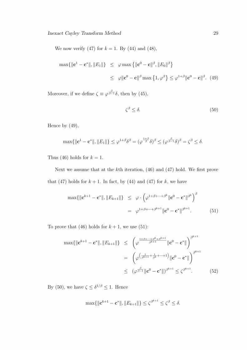
Inexact Cayley Transform Method 29
We now verify (47) for k = 1. By (44) and (48),
max{‖c1 − c∗‖, ‖E1‖} ≤ ϕ max{‖c0 − c‖β, ‖E0‖β
}
≤ ϕ‖c0 − c‖β max{1, ϕβ
} ≤ ϕ1+β‖c0 − c‖β. (49)
Moreover, if we define ζ ≡ ϕβ
β−1 δ, then by (45),
ζβ ≤ δ. (50)
Hence by (49),
max{‖c1 − c∗‖, ‖E1‖} ≤ ϕ1+βδβ = (ϕ1+β
β δ)β ≤ (ϕβ
β−1 δ)β = ζβ ≤ δ.
Thus (46) holds for k = 1.
Next we assume that at the kth iteration, (46) and (47) hold. We first prove
that (47) holds for k + 1. In fact, by (44) and (47) for k, we have
max{‖ck+1 − c∗‖, ‖Ek+1‖} ≤ ϕ ·(ϕ1+β+···+βk‖c0 − c∗‖βk
)β
= ϕ1+β+···+βk+1‖c0 − c∗‖βk+1
. (51)
To prove that (46) holds for k + 1, we use (51):
max{‖ck+1 − c∗‖, ‖Ek+1‖} ≤(
ϕ1+β+···+βk+βk+1
βk+1 ‖c0 − c∗‖)βk+1
=
(ϕ
(1
βk+1 + 1
βk +···+1)‖c0 − c∗‖
)βk+1
≤ (ϕβ
β−1‖c0 − c∗‖)βk+1 ≤ ζβk+1
. (52)
By (50), we have ζ ≤ δ1/β ≤ 1. Hence
max{‖ck+1 − c∗‖, ‖Ek+1‖} ≤ ζβk+1 ≤ ζβ ≤ δ.
Inexact Cayley Transform Method 30
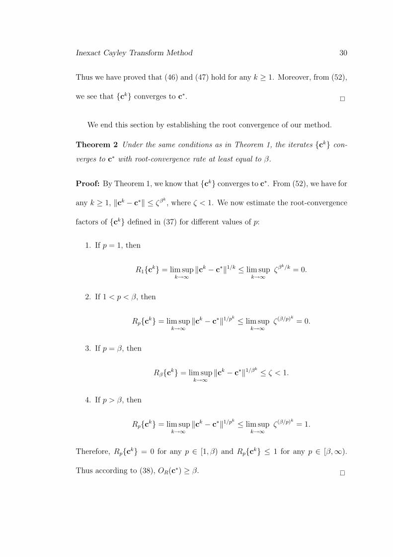
Thus we have proved that (46) and (47) hold for any k ≥ 1. Moreover, from (52),
we see that {ck} converges to c∗.
We end this section by establishing the root convergence of our method.
Theorem 2 Under the same conditions as in Theorem 1, the iterates {ck} con-
verges to c∗ with root-convergence rate at least equal to β.
Proof: By Theorem 1, we know that {ck} converges to c∗. From (52), we have for
any k ≥ 1, ‖ck − c∗‖ ≤ ζβk, where ζ < 1. We now estimate the root-convergence
factors of {ck} defined in (37) for different values of p:
1. If p = 1, then
R1{ck} = lim supk→∞
‖ck − c∗‖1/k ≤ lim supk→∞
ζβk/k = 0.
2. If 1 < p < β, then
Rp{ck} = lim supk→∞
‖ck − c∗‖1/pk ≤ lim supk→∞
ζ(β/p)k
= 0.
3. If p = β, then
Rβ{ck} = lim supk→∞
‖ck − c∗‖1/βk ≤ ζ < 1.
4. If p > β, then
Rp{ck} = lim supk→∞
‖ck − c∗‖1/pk ≤ lim supk→∞
ζ(β/p)k
= 1.
Therefore, Rp{ck} = 0 for any p ∈ [1, β) and Rp{ck} ≤ 1 for any p ∈ [β,∞).
Thus according to (38), OR(c∗) ≥ β.
Inexact Cayley Transform Method 31
5 Numerical Experiments
In this section, we compare the numerical performance of Algorithm I with that
of Algorithm II on two problems. The first one is the inverse Toeplitz eigenvalue
problem, see [6, 27, 31], and the second one is the inverse Sturm-Liouville problem,
see [14] and [8, p. 10]. Our aim is to illustrate the advantage of our method
over Algorithm I in terms of minimizing the oversolving problem and the overall
computational complexity.
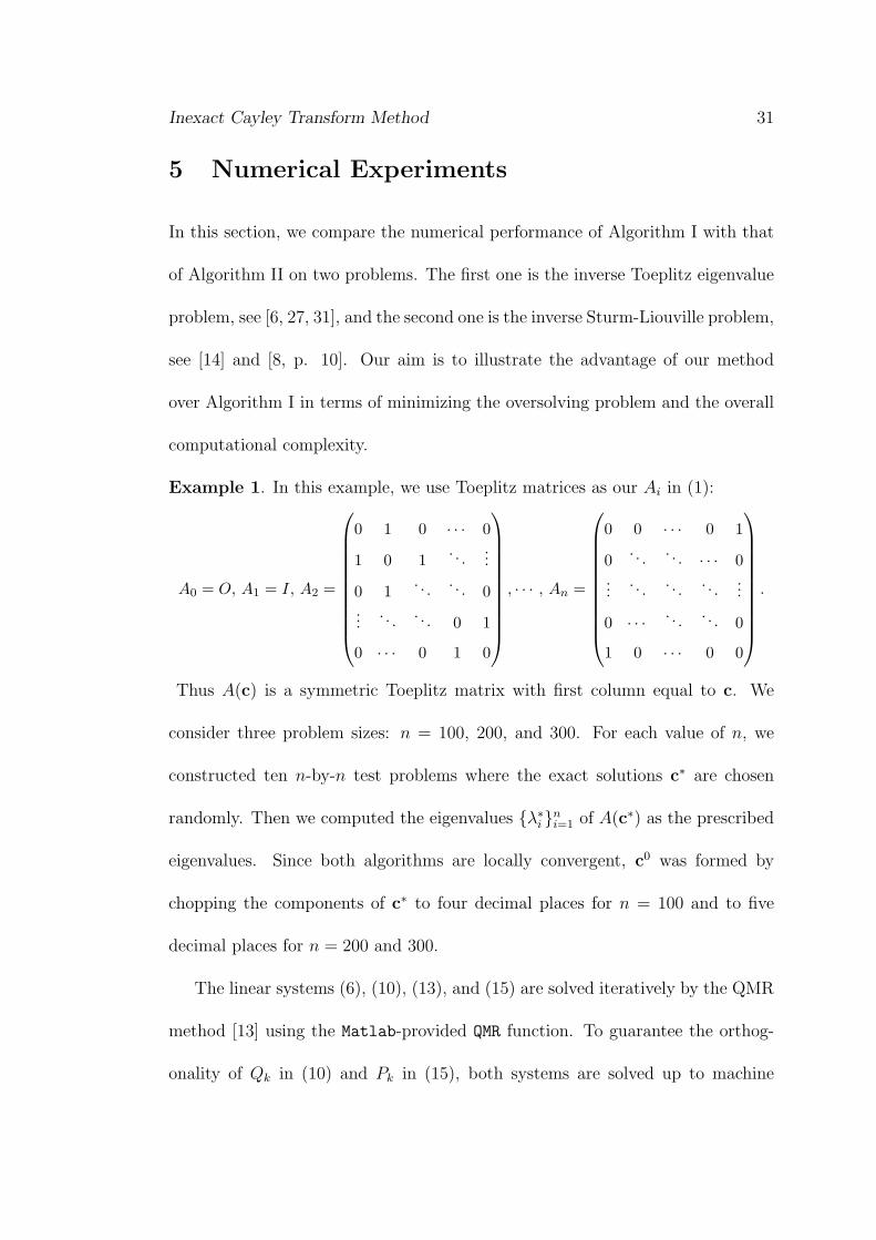
Example 1. In this example, we use Toeplitz matrices as our Ai in (1):
A0 = O, A1 = I, A2 =
0 1 0 · · · 0
1 0 1. . .
...
0 1. . . . . . 0
.... . . . . . 0 1
0 · · · 0 1 0
, · · · , An =
0 0 · · · 0 1
0. . . . . . · · · 0
.... . . . . . . . .
...
0 · · · . . . . . . 0
1 0 · · · 0 0
.
Thus A(c) is a symmetric Toeplitz matrix with first column equal to c. We
consider three problem sizes: n = 100, 200, and 300. For each value of n, we
constructed ten n-by-n test problems where the exact solutions c∗ are chosen
randomly. Then we computed the eigenvalues {λ∗i }ni=1 of A(c∗) as the prescribed
eigenvalues. Since both algorithms are locally convergent, c0 was formed by
chopping the components of c∗ to four decimal places for n = 100 and to five
decimal places for n = 200 and 300.
The linear systems (6), (10), (13), and (15) are solved iteratively by the QMR
method [13] using the Matlab-provided QMR function. To guarantee the orthog-
onality of Qk in (10) and Pk in (15), both systems are solved up to machine
Inexact Cayley Transform Method 32
precision eps (which is ≈ 2.2× 10⁻¹⁶). We use the right-hand side vector as the
initial guess for these two systems.
For the Jacobian systems (6) and (13), we use ck, the iterant at the kth iter-
ation, as the initial guess for the iterative method at the (k + 1)th iteration. We
note that both systems are difficult to solve and one can use preconditioning to
speed up the convergence. Here we have used the Matlab-provided Modified ILU
(MILU) preconditioner: LUINC(A,[drop-tolerance,1,1,1]) since the MILU
preconditioner is one of the most versatile preconditioners for unstructured ma-
trices [9, 17]. The drop tolerance we used is 0.05 for all the three problem sizes.
We emphasize that, we are not attempting to find the best preconditioners for
these systems, but trying to illustrate that preconditioning can be incorporated
into both systems easily.
The inner loop stopping tolerance for (13) is given by (14). For (6) in Algo-
rithm I, we are supposed to solve it up to machine precision eps. Here however,
we first try to solve (6) with a larger stopping tolerance of 10−13 and compare the
two algorithms. Later we will vary this and see how it affects the performance of
Algorithm I. The outer iterations of Algorithms I and II are stopped when
‖QTk A(ck)Qk − Λ∗‖F ≤ 10−10, and ‖P T
k A(ck)Pk − Λ∗‖F ≤ 10−10. (53)
In Table 1, we give the total numbers of outer iterations No averaged over the
ten tests and the average total numbers of inner iterations Ni required for solving
the approximate Jacobian equations. In the table, “I” and “P” respectively mean
Inexact Cayley Transform Method 33
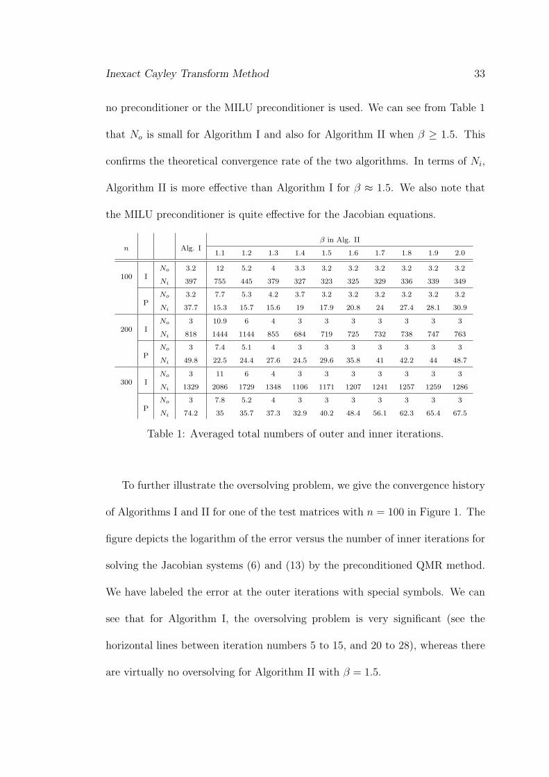
no preconditioner or the MILU preconditioner is used. We can see from Table 1
that No is small for Algorithm I and also for Algorithm II when β ≥ 1.5. This
confirms the theoretical convergence rate of the two algorithms. In terms of Ni,
Algorithm II is more effective than Algorithm I for β ≈ 1.5. We also note that
the MILU preconditioner is quite effective for the Jacobian equations.
β in Alg. IIn Alg. I
1.1 1.2 1.3 1.4 1.5 1.6 1.7 1.8 1.9 2.0
No 3.2 12 5.2 4 3.3 3.2 3.2 3.2 3.2 3.2 3.2100 I
Ni 397 755 445 379 327 323 325 329 336 339 349
No 3.2 7.7 5.3 4.2 3.7 3.2 3.2 3.2 3.2 3.2 3.2P
Ni 37.7 15.3 15.7 15.6 19 17.9 20.8 24 27.4 28.1 30.9
No 3 10.9 6 4 3 3 3 3 3 3 3200 I
Ni 818 1444 1144 855 684 719 725 732 738 747 763
No 3 7.4 5.1 4 3 3 3 3 3 3 3P
Ni 49.8 22.5 24.4 27.6 24.5 29.6 35.8 41 42.2 44 48.7
No 3 11 6 4 3 3 3 3 3 3 3300 I
Ni 1329 2086 1729 1348 1106 1171 1207 1241 1257 1259 1286
No 3 7.8 5.2 4 3 3 3 3 3 3 3P
Ni 74.2 35 35.7 37.3 32.9 40.2 48.4 56.1 62.3 65.4 67.5
Table 1: Averaged total numbers of outer and inner iterations.
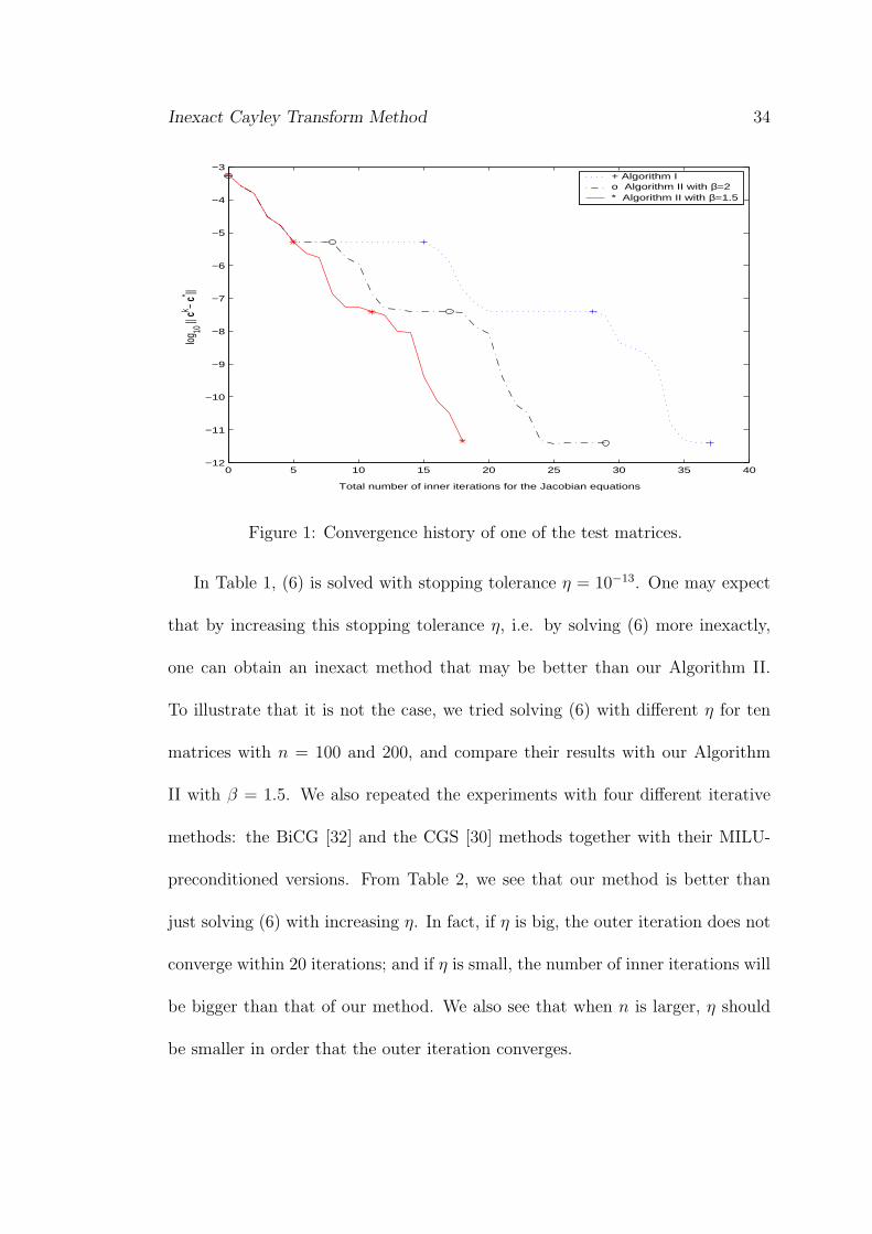
To further illustrate the oversolving problem, we give the convergence history
of Algorithms I and II for one of the test matrices with n = 100 in Figure 1. The
figure depicts the logarithm of the error versus the number of inner iterations for
solving the Jacobian systems (6) and (13) by the preconditioned QMR method.
We have labeled the error at the outer iterations with special symbols. We can
see that for Algorithm I, the oversolving problem is very significant (see the
horizontal lines between iteration numbers 5 to 15, and 20 to 28), whereas there
are virtually no oversolving for Algorithm II with β = 1.5.
Inexact Cayley Transform Method 34
0 5 10 15 20 25 30 35 40−12
−11
−10
−9
−8
−7
−6
−5
−4
−3
Total number of inner iterations for the Jacobian equations
log10
|| ck −
c* || + Algorithm Io Algorithm II with β=2* Algorithm II with β=1.5
Figure 1: Convergence history of one of the test matrices.
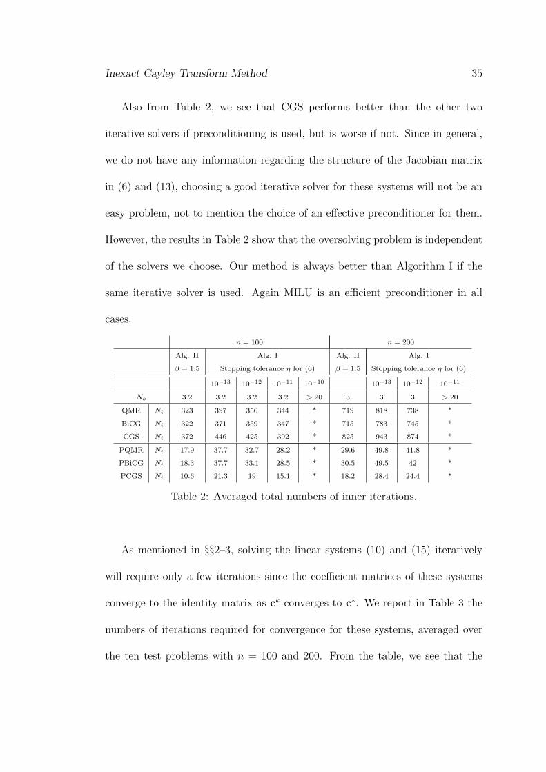
In Table 1, (6) is solved with stopping tolerance η = 10−13. One may expect
that by increasing this stopping tolerance η, i.e. by solving (6) more inexactly,
one can obtain an inexact method that may be better than our Algorithm II.
To illustrate that it is not the case, we tried solving (6) with different η for ten
matrices with n = 100 and 200, and compare their results with our Algorithm
II with β = 1.5. We also repeated the experiments with four different iterative
methods: the BiCG [32] and the CGS [30] methods together with their MILU-
preconditioned versions. From Table 2, we see that our method is better than
just solving (6) with increasing η. In fact, if η is big, the outer iteration does not
converge within 20 iterations; and if η is small, the number of inner iterations will
be bigger than that of our method. We also see that when n is larger, η should
be smaller in order that the outer iteration converges.
Inexact Cayley Transform Method 35
Also from Table 2, we see that CGS performs better than the other two
iterative solvers if preconditioning is used, but is worse if not. Since in general,
we do not have any information regarding the structure of the Jacobian matrix
in (6) and (13), choosing a good iterative solver for these systems will not be an
easy problem, not to mention the choice of an effective preconditioner for them.
However, the results in Table 2 show that the oversolving problem is independent
of the solvers we choose. Our method is always better than Algorithm I if the
same iterative solver is used. Again MILU is an efficient preconditioner in all
cases.
n = 100 n = 200
Alg. II Alg. I Alg. II Alg. I
β = 1.5 Stopping tolerance η for (6) β = 1.5 Stopping tolerance η for (6)
10−13 10−12 10−11 10−10 10−13 10−12 10−11
No 3.2 3.2 3.2 3.2 > 20 3 3 3 > 20
QMR Ni 323 397 356 344 * 719 818 738 *
BiCG Ni 322 371 359 347 * 715 783 745 *
CGS Ni 372 446 425 392 * 825 943 874 *
PQMR Ni 17.9 37.7 32.7 28.2 * 29.6 49.8 41.8 *
PBiCG Ni 18.3 37.7 33.1 28.5 * 30.5 49.5 42 *
PCGS Ni 10.6 21.3 19 15.1 * 18.2 28.4 24.4 *
Table 2: Averaged total numbers of inner iterations.
As mentioned in §§2–3, solving the linear systems (10) and (15) iteratively
will require only a few iterations since the coefficient matrices of these systems
converge to the identity matrix as ck converges to c∗. We report in Table 3 the
numbers of iterations required for convergence for these systems, averaged over
the ten test problems with n = 100 and 200. From the table, we see that the
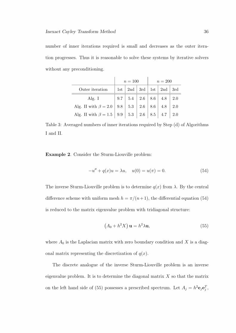
Inexact Cayley Transform Method 36
number of inner iterations required is small and decreases as the outer itera-
tion progresses. Thus it is reasonable to solve these systems by iterative solvers
without any preconditioning.
n = 100 n = 200
Outer iteration 1st 2nd 3rd 1st 2nd 3rd
Alg. I 9.7 5.4 2.6 8.6 4.8 2.0
Alg. II with β = 2.0 9.8 5.3 2.6 8.6 4.8 2.0
Alg. II with β = 1.5 9.9 5.3 2.6 8.5 4.7 2.0
Table 3: Averaged numbers of inner iterations required by Step (d) of Algorithms
I and II.
Example 2. Consider the Sturm-Liouville problem:
−u′′ + q(x)u = λu, u(0) = u(π) = 0. (54)
The inverse Sturm-Liouville problem is to determine q(x) from λ. By the central
difference scheme with uniform mesh h = π/(n+1), the differential equation (54)
is reduced to the matrix eigenvalue problem with tridiagonal structure:
(A0 + h2X
)u = h2λu, (55)
where A0 is the Laplacian matrix with zero boundary condition and X is a diag-
onal matrix representing the discretization of q(x).
The discrete analogue of the inverse Sturm-Liouville problem is an inverse
eigenvalue problem. It is to determine the diagonal matrix X so that the matrix
on the left hand side of (55) possesses a prescribed spectrum. Let Aj = h2ejeTj ,
Inexact Cayley Transform Method 37
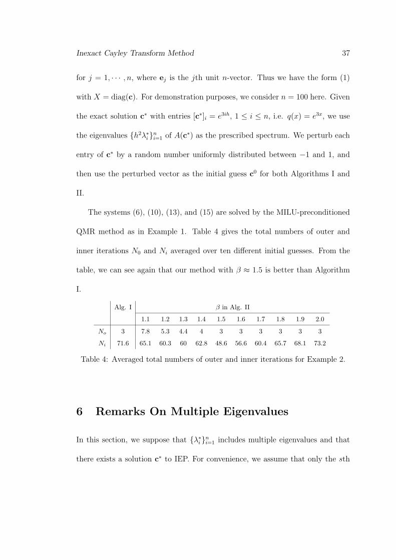
for j = 1, · · · , n, where ej is the jth unit n-vector. Thus we have the form (1)
with X = diag(c). For demonstration purposes, we consider n = 100 here. Given
the exact solution c∗ with entries [c∗]i = e3ih, 1 ≤ i ≤ n, i.e. q(x) = e3x, we use
the eigenvalues {h2λ∗i }ni=1 of A(c∗) as the prescribed spectrum. We perturb each
entry of c∗ by a random number uniformly distributed between −1 and 1, and
then use the perturbed vector as the initial guess c0 for both Algorithms I and
II.
The systems (6), (10), (13), and (15) are solved by the MILU-preconditioned
QMR method as in Example 1. Table 4 gives the total numbers of outer and
inner iterations N0 and Ni averaged over ten different initial guesses. From the
table, we can see again that our method with β ≈ 1.5 is better than Algorithm
I.
Alg. I β in Alg. II
1.1 1.2 1.3 1.4 1.5 1.6 1.7 1.8 1.9 2.0
No 3 7.8 5.3 4.4 4 3 3 3 3 3 3
Ni 71.6 65.1 60.3 60 62.8 48.6 56.6 60.4 65.7 68.1 73.2
Table 4: Averaged total numbers of outer and inner iterations for Example 2.
6 Remarks On Multiple Eigenvalues
In this section, we suppose that {λ∗i }ni=1 includes multiple eigenvalues and that
there exists a solution c∗ to IEP. For convenience, we assume that only the sth
Inexact Cayley Transform Method 38
eigenvalue is multiple, with multiplicity t , i.e.,
λ∗1 < λ∗2 < · · · < λ∗s = λ∗s+1 = · · · = λ∗s+t < λ∗s+t+1 < · · · < λ∗n.
Then it is easy to generalize our remarks to an arbitrary set of multiple eigenval-
ues.
Let us now consider Algorithm II. Equation (13) still holds, regardless of the
eigenvalue multiplicities. The off-diagonal equations in Substep (c) of Step 2 is
not true for s ≤ i 6= j ≤ s + t as before. A reasonable course is to set
[Yk]ij = 0, s ≤ i 6= j ≤ s + t.
With this choice, following the proof of Theorems 1 and 2, we can show that the
iterates {ck} converge to c∗ with root-convergence rate at least β.
Acknowledgment: We would like to thank the referees for their insightful and
valuable comments.
References
[1] A. Andrew, Some Recent Developments in Inverse Eigenvalue Problems, in
Computational Techniques and Applications, CTAC93, D. Stewart, H. Gard-
ner, and D. Singleton, eds., World Scientific, Singapore, 1994, pp. 94–102.
[2] E. Allgower and K. Georg, Continuation and Path Following, Acta Numer.,
(1993), pp. 1–64.
Inexact Cayley Transform Method 39
[3] C. Byrnes, Pole Placement by Output Feedback, in Three Decades of Math-
ematics Systems Theory, Lecture Notes in Control and Inform. Sci. 135,
Springer-Verlag, New York, 1989, pp. 31–78.
[4] R. Chan, H. Chung, and S. Xu, The Inexact Newton-Like Method for Inverse
Eigenvalue Problem, BIT, 43 (2003), pp. 7–20.
[5] M. Chu, Inverse Eigenvalue Problems, SIAM Rev., 40 (1998), pp. 1–39.
[6] M. Chu, On a Newton Method for the Inverse Toeplitz Eigenvalue Problem,
preprint available at http://www4.ncsu.edu/˜mtchu/Research/Papers/itep.ps.
[7] M. Chu, Numerical Methods for Inverse Singular Value Problems, SIAM J.
Numer. Anal., 29 (1992), pp. 885–903.
[8] M. Chu and G. Golub, Structured Inverse Eigenvalue Problems, Acta Numer.,
11 (2002), pp. 1–71.
[9] T. Dupont, R. Kendall, and H. Rachford, JR., An Approximate Factoriza-
tion Procedure for Solving Self-adjoint Elliptic Difference Equations, SIAM J.
Numer. Anal., 5 (1968), pp. 559–573.
[10] S. Eisenstat and H. Walker, Choosing the Forcing Terms in an Inexact New-
ton Method, SIAM J. Sci. Comput., 17 (1996), pp. 16–32.
[11] S. Elhay and Y. Ram, An Affine Inverse Eigenvalue Problem, Inverse Prob-
lems, 18 (2002), pp. 455–466.
Inexact Cayley Transform Method 40
[12] D. Fokkema, G. Sleijpen, and H. van der Vorst, Accelerated Inexact Newton
Schemes for Large Systems of Nonlinear Equations, SIAM J. Sci. Comput.,
19 (1998), pp. 657–674.
[13] R. Freund and N. Nachtigal, QMR: A Quasi-Minimal Residual Method for
Non-Hermitian Linear Systems, Numer. Math., 60 (1991), pp. 315–339.
[14] S. Friedland, J. Nocedal, and M. Overton, The Formulation and Analysis of
Numerical Methods for Inverse Eigenvalue Problems, SIAM J. Numer. Anal.,
24 (1987), pp. 634–667.
[15] G. Gladwell, Inverse Problems in Vibration, Appl. Mech. Rev., 39 (1986),
pp. 1013–1018.
[16] G. Gladwell, Inverse Problems in Vibration, II, Appl. Mech. Rev., 49 (1996),
pp. 25–34.
[17] I. Gustafsson, A Class of First Order Factorizations, BIT, 18 (1978), pp.
142–156.
[18] O. Hald, On Discrete and Numerical Inverse Sturm-Liouville Problems,
Ph.D. thesis, New York University, New York, 1972.
[19] K. Joseph, Inverse Eigenvalue Problem in Structural Design, AIAA Ed. Ser.,
30 (1992), pp. 2890–2896.
Inexact Cayley Transform Method 41
[20] N. Li, A Matrix Inverse Eigenvalue Problem and Its Application, Linear
Algebra Appl., 266 (1997), pp. 143–152.
[21] M. McCarthy, Recovery of a Density From the Eigenvalues of a Nonhomo-
geneous Membrane, Proceedings of the Third International Conference on
Inverse Problems in Engineering: Theory and Practice, Port Ludlow, Wash-
ington, June 13–18, 1999.
[22] B. Morini, Convergence Behaviour of Inexact Newton Methods, Math. Com-
put., 68 (1999), pp. 1605–1613.
[23] M. Muller, An Inverse Eigenvalue Problem: Computing B-Stable Runge-
Kutta Methods Having Real Poles, BIT, 32 (1992), pp. 676–688.
[24] M. Neher, Ein Einschlieβungsverfahren fur das Inverse Dirichletproblem,
Doctoral thesis, University of Karlsruhe, Karlsruhe, Germany, 1993.
[25] J. Ortega and W. Rheinboldt, Iterative Solution of Nonlinear Equations in
Several Variables, Academic Press, 1970.
[26] R. Parker and K. Whaler, Numerical Methods for Establishing Solutions
to the Inverse Problem of Electromagnetic Induction, J. Geophys. Res., 86
(1981), pp. 9574–9584.
[27] J. Peinado and A. Vidal, A New Parallel Approach to the Toeplitz Inverse
Eigenproblem Using Newton-like Methods, Lecture Notes in Computer Sci-
ence, 1981/2001, Springer-Verlag, 2003, pp. 355–368.
Inexact Cayley Transform Method 42
[28] M. Ravi, J. Rosenthal, and X. Wang, On Decentralized Dynamic Pole Place-
ment and Feedback Stabilization, IEEE Trans. Automat. Control, 40 (1995),
pp. 1603–1614.
[29] V. Scholtyssek, Solving Inverse Eigenvalue Problems by a Projected Newton
Method, Numer. Funct. Anal. Optim., 17 (1996), pp. 925–944.
[30] P. Sonneveld, CGS: A Fast Lanczos-Type Solver for Nonsymmetric Linear
Systems, SIAM J. Sci. Stat. Comput., 10 (1989), pp. 36–52.
[31] W. Trench, Numerical Solution of the Inverse Eigenvalue Problem for Real
Symmmetric Toeplitz Matrices, SIAM J. Sci. Comput., 18 (1997), pp. 1722–
1736.
[32] H. van der Vorst, BiCGSTAB: A Fast and Smoothly Converging Variant of
the Bi-CG for the Solution of Nonsymmetric Linear Systems, SIAM J. Sci.
and Stat. Comp., 13 (1992), pp. 631–644.
[33] S. Xu, An Introduction to Inverse Algebraic Eigenvalue Problems, Peking
University Press and Vieweg Publishing, 1998.
The Solvability Conditions for the Inverse
Eigenvalue Problem of Hermitian and
Generalized Skew-Hamiltonian Matrices and Its
Approximation
Abstract
In this paper, we first consider the inverse eigenvalue problem as fol-
lows: Find a matrix A with specified eigen-pairs, where A is a Hermitian
and generalized skew-Hamiltonian matrix. The sufficient and necessary
conditions are obtained, and a general representation of such a matrix is
presented. We denote the set of such matrices by LS . Then the best ap-
proximation problem for the inverse eigenproblem is discussed. That is:
Given an arbitrary A, find a matrix A∗ ∈ LS which is nearest to A in
the Frobenius norm. We show that the best approximation is unique and
provide an expression for this nearest matrix.
1 Introduction
Let J ∈ Rn×n be an orthogonal skew-symmetric matrix, i.e. J ∈ Rn×n satisfies
that JT J = JJT = In, JT = −J . Then we have J2 = −In and n = 2k, k ∈ N .
In the following, we give the definitions of generalized Hamiltonian and general-
43
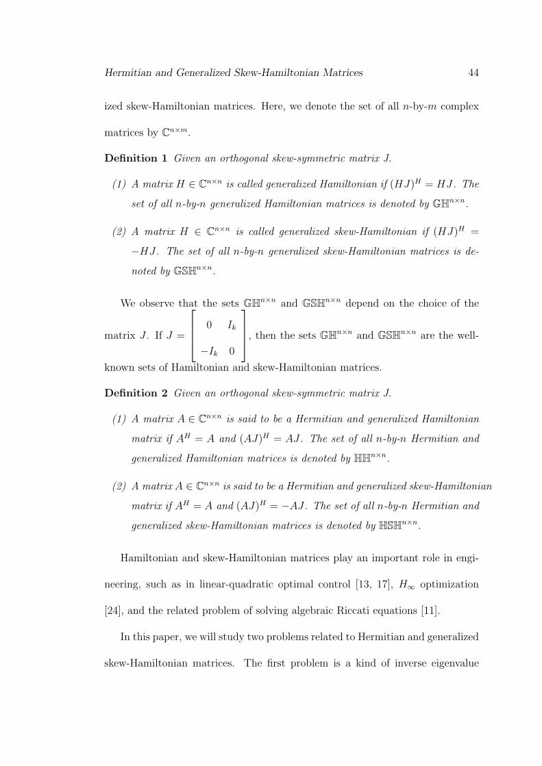
Hermitian and Generalized Skew-Hamiltonian Matrices 44
ized skew-Hamiltonian matrices. Here, we denote the set of all n-by-m complex
matrices by Cn×m.
Definition 1 Given an orthogonal skew-symmetric matrix J.
(1) A matrix H ∈ Cn×n is called generalized Hamiltonian if (HJ)H = HJ . The
set of all n-by-n generalized Hamiltonian matrices is denoted by GHn×n.
(2) A matrix H ∈ Cn×n is called generalized skew-Hamiltonian if (HJ)H =
−HJ . The set of all n-by-n generalized skew-Hamiltonian matrices is de-
noted by GSHn×n.
We observe that the sets GHn×n and GSHn×n depend on the choice of the
matrix J . If J =
0 Ik
−Ik 0
, then the sets GHn×n and GSHn×n are the well-
known sets of Hamiltonian and skew-Hamiltonian matrices.
Definition 2 Given an orthogonal skew-symmetric matrix J.
(1) A matrix A ∈ Cn×n is said to be a Hermitian and generalized Hamiltonian
matrix if AH = A and (AJ)H = AJ . The set of all n-by-n Hermitian and
generalized Hamiltonian matrices is denoted by HHn×n.
(2) A matrix A ∈ Cn×n is said to be a Hermitian and generalized skew-Hamiltonian
matrix if AH = A and (AJ)H = −AJ . The set of all n-by-n Hermitian and
generalized skew-Hamiltonian matrices is denoted by HSHn×n.
Hamiltonian and skew-Hamiltonian matrices play an important role in engi-
neering, such as in linear-quadratic optimal control [13, 17], H∞ optimization
[24], and the related problem of solving algebraic Riccati equations [11].
In this paper, we will study two problems related to Hermitian and generalized
skew-Hamiltonian matrices. The first problem is a kind of inverse eigenvalue
Hermitian and Generalized Skew-Hamiltonian Matrices 45
problems. For decades, structured inverse eigenvalue problems have been of great
value for many applications, see for instance the expository papers [7, 22]. There
are also different types of inverse eigenproblem, for instances multiplicative type
and additive type [22, Chapter 4]. In what follows, we consider the following type
of inverse eigenproblem which appeared in the design of Hopfield neural networks
[6, 12].
Problem I. Given X = [x1,x2, . . . ,xm] ∈ Cn×m and Λ = diag(λ1, . . . , λm) ∈
Cm×m, find a Hermitian and generalized skew-Hamiltonian matrix A in HSHn×n
such that AX = XΛ.
We note from the above definition that the eigenvalues of a Hermitian and
generalized skew-Hamiltonian matrix are real numbers. Hence we have Λ =
diag(λ1, . . . , λm) ∈ Rm×m.
The second problem we consider in this paper is the problem of best approx-
imation:
Problem II. Let LS be the solution set of Problem I. Given a matrix A ∈ Cn×n,
find A∗ ∈ LS such that
‖A− A∗‖ = minA∈LS
‖A− A‖,
where ‖ · ‖ is the Frobenius norm.
The best approximation problem occurs frequently in experimental design,
see for instance [14, p.123]. Here the matrix A may be a matrix obtained from
Hermitian and Generalized Skew-Hamiltonian Matrices 46
experiments, but it may not satisfy the structural requirement (Hermitian and
generalized skew-Hamiltonian) and/or spectral requirement (having eigenpairs X
and Λ). The best estimate A∗ is the matrix that satisfies both restrictions and is
the best approximation of A in the Frobenius norm, see for instance [2, 3, 10].
Problems I and II have been solved for different classes of structured matrices,
see for instance [21, 23]. In this paper, we extend the results in [23] to the class of
Hermitian and generalized skew-Hamiltonian matrices. We first give a solvability
condition for Problem I and also the form of its general solution. Then in the
case when Problem I is solvable, we show that Problem II has a unique solution
and give a formula for the minimizer A∗.
In this paper, the notations are as follows. Let U(n) be the set of all n-by-n
unitary matrices, and Hn×n denote the set of all n-by-n Hermitian matrices. We
denote the transpose, conjugate transpose and the Moore-Penrose generalized
inverse of a matrix A by AT , AH and A+ respectively, and the identity matrix of
order n by In. We define the inner product in space Cn×m by
(A,B) = tr(AHB), ∀A,B ∈ Cn×m.
Then Cn×m is a Hilbert inner product space. The norm of a matrix generated by
the inner product space is the Frobenius norm.
This paper is outlined as follows. In §2 we first discuss the structure of the
set HSHn×n, and then present the solvability conditions and provide the general
solution formula for Problem I. In §3 we first show the existence and uniqueness
Hermitian and Generalized Skew-Hamiltonian Matrices 47
of the solution for Problem II, and then derive an expression of the solution when
the solution set LS is nonempty, and finally propose an algorithm to compute the
solution to Problem II. In §4 we give some illustrative numerical examples.
2 Solvability Conditions of Problem I
We first discuss the structure of HSHn×n. In what follows, we always assume that
n = 2k, k ∈ N . By the definition of HSHn×n, we have the following statement.
Lemma 1 Let A ∈ Cn×n, then A ∈ HSHn×n if and only if AH = A, AJ−JA = 0.
Since J is orthogonal skew-symmetric, J is normal and skew-symmetric and
then has only two multiple eigenvalues i and −i with multiplicity k respectively,
where i denotes the the imaginary unit, i.e. i2 = −1. Thus we can easily show
the following lemma.
Lemma 2 Let J ∈ Rn×n be orthogonal skew-symmetric, then there exists a ma-
trix U ∈ U(n) such that
J = U
i · Ik 0
0 −i · Ik
UH . (1)
By the above two lemmas, we have the following result for the structure of
HSHn×n.
Theorem 1 Let A ∈ Cn×n and the spectral decomposition of J be given as (1).
Then A ∈ HSHn×n if and only if
A = U
A11 0
0 A22
UH , A11, A22 ∈ Hk×k. (2)
Hermitian and Generalized Skew-Hamiltonian Matrices 48
Proof: If A ∈ HSHn×n, then by Lemma 1 and (1), we obtain
UHAU
i · Ik 0
0 −i · In−k
+
i · Ik 0
0 −i · In−k
UHAU = 0. (3)
Since AH = A, then UHAU ∈ Hn×n. Let
A = U
A11 A12
AH12 A22
UH , A11 ∈ Hk×k, A22 ∈ Hk×k.
Substituting it into (3) yields (2).
On the other hand, if A can be expressed as (2), then, obviously, AH = A,
AJ − JA = 0. By Lemma 1, A ∈ HSHn×n.
We now investigate the solvability of Problem I. We need the following lemma,
see for instance [19].
Lemma 3 [19, Lemma 1.4] Let B, C ∈ Cn×m be given. Then HB = C has a
solution in Hn×n if and only if
C = CB+B and (BB+CB+)H = BB+CB+.
In this case the general solution can be expressed by
Y = CB+ + (B+)HCH − (B+)HCHBB+ + (I −BB+)Z(I −BB+),
where Z ∈ Hn×n is arbitrary.
Then we can establish the solvability of Problem I as follows.
Theorem 2 Given X ∈ Cn×m, Λ = diag(λ1, . . . , λm) ∈ Rm×m. Let
UHX =
X1
X2
, X1, X2 ∈ Ck×m. (4)
Hermitian and Generalized Skew-Hamiltonian Matrices 49
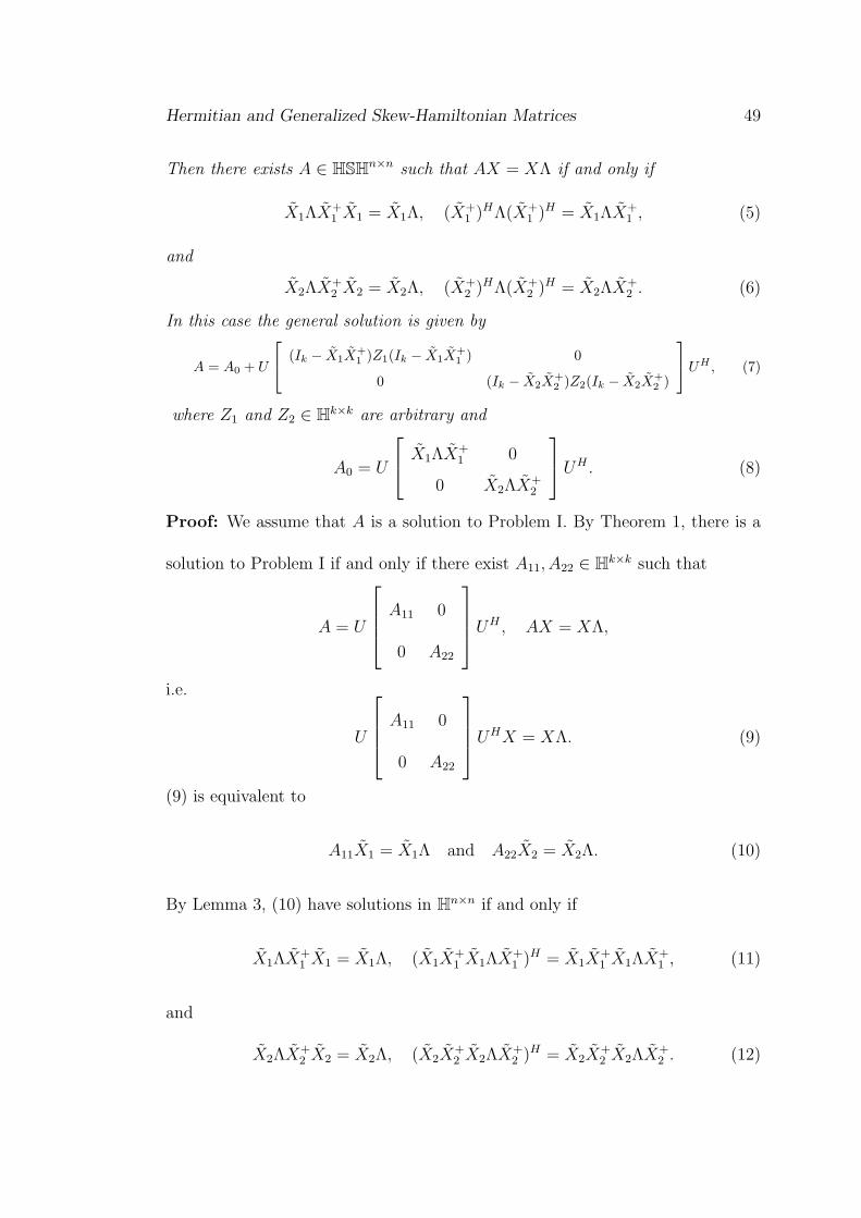
Then there exists A ∈ HSHn×n such that AX = XΛ if and only if
X1ΛX+1 X1 = X1Λ, (X+
1 )HΛ(X+1 )H = X1ΛX+
1 , (5)
and
X2ΛX+2 X2 = X2Λ, (X+
2 )HΛ(X+2 )H = X2ΛX+
2 . (6)
In this case the general solution is given by
A = A0 + U
(Ik − X1X
+1 )Z1(Ik − X1X
+1 ) 0
0 (Ik − X2X+2 )Z2(Ik − X2X
+2 )
UH , (7)
where Z1 and Z2 ∈ Hk×k are arbitrary and
A0 = U
X1ΛX+
1 0
0 X2ΛX+2
UH . (8)
Proof: We assume that A is a solution to Problem I. By Theorem 1, there is a
solution to Problem I if and only if there exist A11, A22 ∈ Hk×k such that
A = U
A11 0
0 A22
UH , AX = XΛ,
i.e.
U
A11 0
0 A22
UHX = XΛ. (9)
(9) is equivalent to
A11X1 = X1Λ and A22X2 = X2Λ. (10)
By Lemma 3, (10) have solutions in Hn×n if and only if
X1ΛX+1 X1 = X1Λ, (X1X
+1 X1ΛX+
1 )H = X1X+1 X1ΛX+
1 , (11)
and
X2ΛX+2 X2 = X2Λ, (X2X
+2 X2ΛX+
2 )H = X2X+2 X2ΛX+
2 . (12)
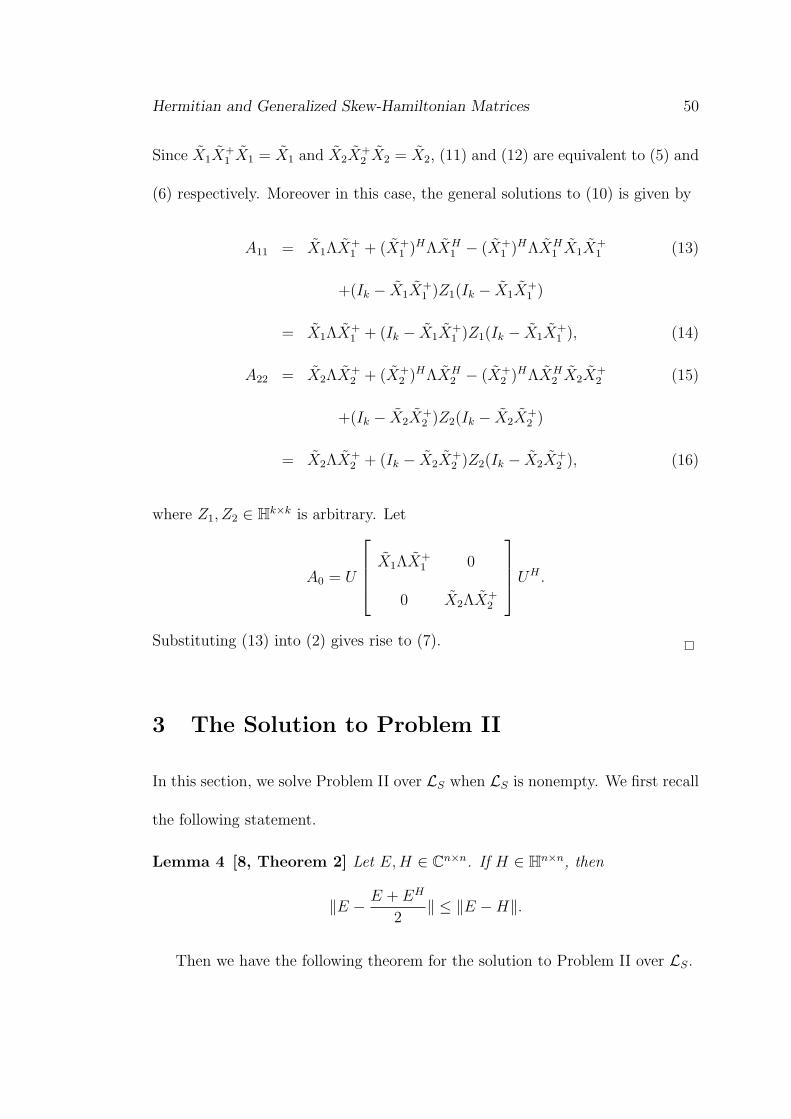
Hermitian and Generalized Skew-Hamiltonian Matrices 50
Since X1X+1 X1 = X1 and X2X
+2 X2 = X2, (11) and (12) are equivalent to (5) and
(6) respectively. Moreover in this case, the general solutions to (10) is given by
A11 = X1ΛX+1 + (X+
1 )HΛXH1 − (X+
1 )HΛXH1 X1X
+1 (13)
+(Ik − X1X+1 )Z1(Ik − X1X
+1 )
= X1ΛX+1 + (Ik − X1X
+1 )Z1(Ik − X1X
+1 ), (14)
A22 = X2ΛX+2 + (X+
2 )HΛXH2 − (X+
2 )HΛXH2 X2X
+2 (15)
+(Ik − X2X+2 )Z2(Ik − X2X
+2 )
= X2ΛX+2 + (Ik − X2X
+2 )Z2(Ik − X2X
+2 ), (16)
where Z1, Z2 ∈ Hk×k is arbitrary. Let
A0 = U
X1ΛX+1 0
0 X2ΛX+2
UH .
Substituting (13) into (2) gives rise to (7).
3 The Solution to Problem II
In this section, we solve Problem II over LS when LS is nonempty. We first recall
the following statement.
Lemma 4 [8, Theorem 2] Let E, H ∈ Cn×n. If H ∈ Hn×n, then
‖E − E + EH
2‖ ≤ ‖E −H‖.
Then we have the following theorem for the solution to Problem II over LS.
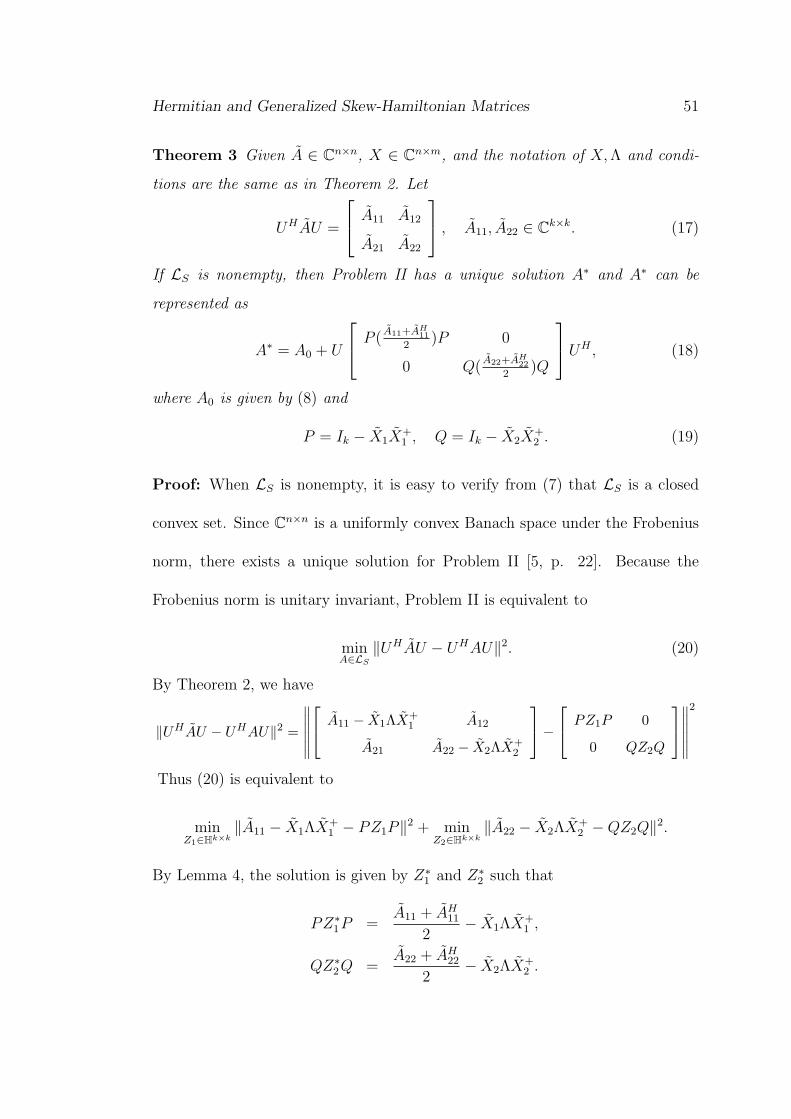
Hermitian and Generalized Skew-Hamiltonian Matrices 51
Theorem 3 Given A ∈ Cn×n, X ∈ Cn×m, and the notation of X, Λ and condi-
tions are the same as in Theorem 2. Let
UHAU =
A11 A12
A21 A22
, A11, A22 ∈ Ck×k. (17)
If LS is nonempty, then Problem II has a unique solution A∗ and A∗ can be
represented as
A∗ = A0 + U
P (
A11+AH11
2)P 0
0 Q(A22+AH
22
2)Q
UH , (18)
where A0 is given by (8) and
P = Ik − X1X+1 , Q = Ik − X2X
+2 . (19)
Proof: When LS is nonempty, it is easy to verify from (7) that LS is a closed
convex set. Since Cn×n is a uniformly convex Banach space under the Frobenius
norm, there exists a unique solution for Problem II [5, p. 22]. Because the
Frobenius norm is unitary invariant, Problem II is equivalent to
minA∈LS
‖UHAU − UHAU‖2. (20)
By Theorem 2, we have
‖UHAU − UHAU‖2 =
∥∥∥∥∥∥
A11 − X1ΛX+
1 A12
A21 A22 − X2ΛX+2
−
PZ1P 0
0 QZ2Q
∥∥∥∥∥∥
2
Thus (20) is equivalent to
minZ1∈Hk×k
‖A11 − X1ΛX+1 − PZ1P‖2 + min
Z2∈Hk×k‖A22 − X2ΛX+
2 −QZ2Q‖2.
By Lemma 4, the solution is given by Z∗1 and Z∗
2 such that
PZ∗1P =
A11 + AH11
2− X1ΛX+
1 ,
QZ∗2Q =
A22 + AH22
2− X2ΛX+
2 .
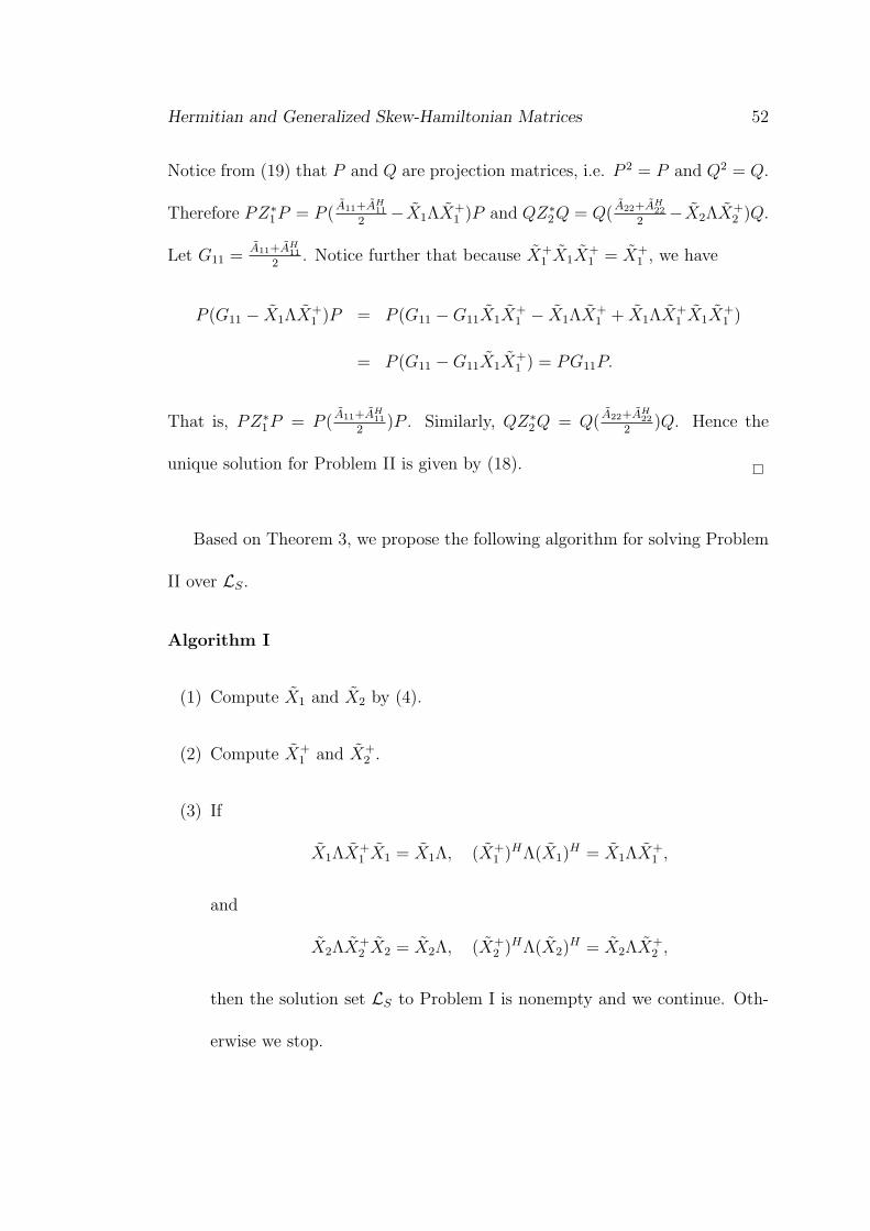
Hermitian and Generalized Skew-Hamiltonian Matrices 52
Notice from (19) that P and Q are projection matrices, i.e. P 2 = P and Q2 = Q.
Therefore PZ∗1P = P (
A11+AH11
2−X1ΛX+
1 )P and QZ∗2Q = Q(
A22+AH22
2−X2ΛX+
2 )Q.
Let G11 =A11+AH
11
2. Notice further that because X+
1 X1X+1 = X+
1 , we have
P (G11 − X1ΛX+1 )P = P (G11 −G11X1X
+1 − X1ΛX+
1 + X1ΛX+1 X1X
+1 )
= P (G11 −G11X1X+1 ) = PG11P.
That is, PZ∗1P = P (
A11+AH11
2)P . Similarly, QZ∗
2Q = Q(A22+AH
22
2)Q. Hence the
unique solution for Problem II is given by (18).
Based on Theorem 3, we propose the following algorithm for solving Problem
II over LS.
Algorithm I
(1) Compute X1 and X2 by (4).
(2) Compute X+1 and X+
2 .
(3) If
X1ΛX+1 X1 = X1Λ, (X+
1 )HΛ(X1)H = X1ΛX+
1 ,
and
X2ΛX+2 X2 = X2Λ, (X+
2 )HΛ(X2)H = X2ΛX+
2 ,
then the solution set LS to Problem I is nonempty and we continue. Oth-
erwise we stop.
Hermitian and Generalized Skew-Hamiltonian Matrices 53
(4) Compute A11 and A22 by (17).
(5) Compute G11 =A11+AH
11
2and G22 =
A22+AH22
2.
(6) Compute
M11 = X1ΛX+1 + G11 −G11X1X
+1 − X1X
+1 G11 − X1X
+1 G11X1X
+1 ,
M22 = X2ΛX+2 + G22 −G22X2X
+2 − X2X
+2 G22 + X2X
+2 G22X2X
+2 .
(7) Compute A∗ = U
M11 0
0 M22
UH .
Now, we consider the computational complexity of our algorithm. We observe
from Lemma 2 that, for different choice of J , the structure of U ∈ U(n) may be
varied. Thus the total computational complexity may be changed.
We first consider the case when given a fixed J with U ∈ U(n) dense. For
Step (1), since U is dense, it requires O(n2m) operations to compute X1 and X2.
For Step (2), using singular value decomposition to compute X+1 and X+
2 requires
O(n2m + m3) operations. Step (3) obviously requires O(n2m) operations. For
Step(4), because of the density of U , the operations required is O(n3). Step(5) re-
quires O(n) operations only. For Step(6), if we compute GiiXiX+i as [(GiiXi)X
+i ],
XiX+i Gii as [Xi(X
+i Gii)], and XiX
+i GiiXiX
+i as {Xi[(X
+i (GiiXi))X
+i ]} , then
the cost will only be of O(n2m) operations. Finally, because of the density of U
again, Step (7) requires O(n3) operations. Thus the total cost of the algorithm
is O(n3 + n2m + m3).
Hermitian and Generalized Skew-Hamiltonian Matrices 54
In particular, if we choose that
J =
0 Ik
−Ik 0
, U =
1√2
Ik Ik
i · Ik −i · Ik
∈ U(n).
Then, because of the sparsity of U , Steps (1), (4) and (7) will require O(nm),
O(n2) and O(n2) respectively. Therefore the total complexity of the algorithm is
O(n2m + m3).
Finally, we remark that in practice, m ¿ n. In addition, it is easy to verify
that our algorithm is stable.
4 Numerical Experiments
In this section, we will give some numerical examples to illustrate our results.
All the tests are performed by MATLAB which has a machine precision around
10−16. In the following, we let n = 2k, k ∈ N and J =
0 Ik
−Ik 0
. Then it is
clear that the spectral decomposition of J is given by
J = U
i · Ik 0
0 −i · Ik
UH ,
where U = 1√2
Ik Ik
i · Ik −i · Ik
, UHU = UUH = In.
Hermitian and Generalized Skew-Hamiltonian Matrices 55
Example 1. We choose a random matrix A in HSHn×n:
A =
1.9157 -0.5359 + 5.5308i 0 + 0.0596i 4.2447 + 0.1557i
-0.5359 - 5.5308i -0.5504 -4.2447 + 0.1557i 0 + 0.8957i
0 - 0.0596i -4.2447 - 0.1557i 1.9157 -0.5359 + 5.5308i
4.2447 - 0.1557i 0 - 0.8957i -0.5359 - 5.5308i -0.5504
.
Then the eigenvalues of A are −9.7331, −0.4090, 2.7296, and 10.1431. We let
{x1,x2,x3,x4} denote the eigenvectors of A associated with −9.7331, −0.4090,
2.7296, and 10.1431 respectively. Now we take X = [x1,x2,x3,x4], i.e.
X =
-0.4554 - 0.0322i 0.3324 + 0.0983i 0.5910 + 0.1747i 0.5386 + 0.0381i
0.0000 - 0.5399i -0.0000 + 0.6163i -0.0000 - 0.3466i 0.0000 - 0.4566i
0.0322 - 0.4554i 0.0983 - 0.3324i 0.1747 - 0.5910i -0.0381 + 0.5386i
0.5399 0.6163 -0.3466 0.4566
and
Λ =
-9.7331 0 0 0
0 -0.4090 0 0
0 0 2.7296 0
0 0 0 10.1431
.
Given such X and Λ, it is easy to see that there exists a solution for Problem
I, i.e. A. Thus LS is nonempty. If we perturb A to obtain a matrix A(ε) =
A + ε · C 6∈ HSHn×n, where
C =
0.2476 + 0.7668i 0.3006 + 0.8790i 0.8569 + 0.4963i 0.2968 + 0.3608i
0.4358 + 0.5740i 0.2659 + 0.9058i 0.2429 + 0.3921i 0.3903 + 0.3135i
0.9776 + 0.7098i 0.1334 + 0.0886i 0.1949 + 0.5583i 0.1873 + 0.7436i
0.8600 + 0.8126i 0.7425 + 0.3055i 0.3908 + 0.6318i 0.8957 + 0.2838i
,
then the conditions in Theorem 2 and Theorem 3 are satisfied. Using Algorithm I
in §3, we get the solution A∗(ε) of Theorem 3 corresponding to A(ε). In Figure 1,
we plot the following two quantities for ε from 10−10 to 1010: log10 ‖A(ε)−A∗(ε)‖
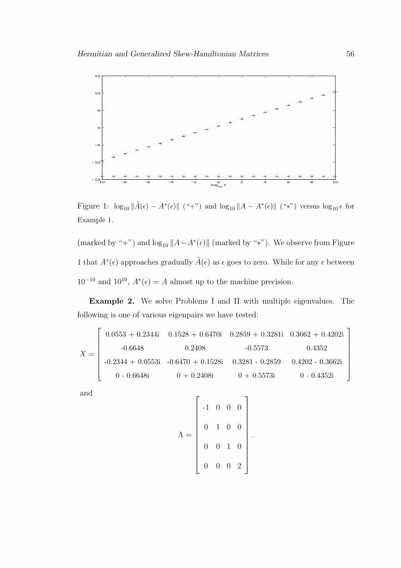
Hermitian and Generalized Skew-Hamiltonian Matrices 56
−10 −8 −6 −4 −2 0 2 4 6 8 10−15
−10
−5
0
5
10
15
log10
ε
Figure 1: log10 ‖A(ε) − A∗(ε)‖ (“+”) and log10 ‖A − A∗(ε)‖ (“∗”) versus log10 ε for
Example 1.
(marked by “+”) and log10 ‖A−A∗(ε)‖ (marked by “∗”). We observe from Figure
1 that A∗(ε) approaches gradually A(ε) as ε goes to zero. While for any ε between
10−10 and 1010, A∗(ε) = A almost up to the machine precision.
Example 2. We solve Problems I and II with multiple eigenvalues. The
following is one of various eigenpairs we have tested:
X =
0.0553 + 0.2344i 0.1528 + 0.6470i 0.2859 + 0.3281i 0.3662 + 0.4202i
-0.6648 0.2408 -0.5573 0.4352
-0.2344 + 0.0553i -0.6470 + 0.1528i 0.3281 - 0.2859 0.4202 - 0.3662i
0 - 0.6648i 0 + 0.2408i 0 + 0.5573i 0 - 0.4352i
and
Λ =
-1 0 0 0
0 1 0 0
0 0 1 0
0 0 0 2
.
Hermitian and Generalized Skew-Hamiltonian Matrices 57
Given such X and Λ, it is easy to verify that there exists a solution for Problem
I, i.e.
A =
1.1946 0.2329 + 0.4945i 0 + 0.4266i 0.1288 + 0.0858i
0.2329 - 0.4945i 0.3054 -0.1288 + 0.0858i 0 + 1.0734i
0 - 0.4266i -0.1288 - 0.0858i 1.1946 0.2329 + 0.4945i
0.1288 - 0.0858i 0 - 1.0734i 0.2329 - 0.4945i 0.3054
.
Thus LS is nonempty. We now perturb A to obtain a matrix A(ε) = A + ε ·F 6∈HSHn×n, where
F =
0.8408 + 0.4910i 0.7168 + 0.5550i 0.9106 + 0.6066i 0.8739 + 0.6959i
0.6463 + 0.9427i 0.8112 + 0.5147i 0.2761 + 0.3202i 0.7105 + 0.7889i
0.0559 + 0.5107i 0.1534 + 0.7272i 0.9571 + 0.4688i 0.9746 + 0.9407i
0.2057 + 0.3490i 0.0864 + 0.1896i 0.7400 + 0.7850i 0.1543 + 0.6763i
.
Then the conditions in Theorems 2 and 3 are satisfied. Using Algorithm I in
§3, we get the solution A∗(ε) of Theorem 3 corresponding to A(ε). In Figure 2,
we plot the following two quantities for ε from 10−10 to 1010: log10 ‖A(ε)−A∗(ε)‖
(marked by “+”) and log10 ‖A−A∗(ε)‖ (marked by “∗”). We can see from Figure
2 that A∗(ε) approximates to A(ε) as ε goes to zero. However, for any ε between
10−10 and 1010, A∗(ε) = A almost up to the machine precision.
Example 3. Let T (1 : n) denote a n-by-n Hermitian Toeplitz matrix whose
first row is (1, 2+2 ·i, . . . , n+n ·i), and T (1 : 1/n) be a n-by-n Hermitian Toeplitz
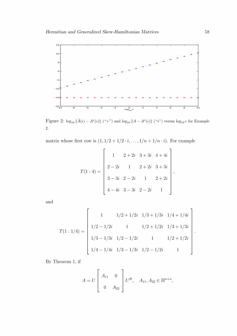
Hermitian and Generalized Skew-Hamiltonian Matrices 58
−10 −8 −6 −4 −2 0 2 4 6 8 10−20
−15
−10
−5
0
5
10
15
log10
ε
Figure 2: log10 ‖A(ε)− A∗(ε)‖ (“+”) and log10 ‖A− A∗(ε)‖ (“∗”) versus log10 ε for Example
2.
matrix whose first row is (1, 1/2 + 1/2 · i, . . . , 1/n + 1/n · i). For example
T (1 : 4) =
1 2 + 2i 3 + 3i 4 + 4i
2− 2i 1 2 + 2i 3 + 3i
3− 3i 2− 2i 1 2 + 2i
4− 4i 3− 3i 2− 2i 1
,
and
T (1 : 1/4) =
1 1/2 + 1/2i 1/3 + 1/3i 1/4 + 1/4i
1/2− 1/2i 1 1/2 + 1/2i 1/3 + 1/3i
1/3− 1/3i 1/2− 1/2i 1 1/2 + 1/2i
1/4− 1/4i 1/3− 1/3i 1/2− 1/2i 1
.
By Theorem 1, if
A = U
A11 0
0 A22
UH , A11, A22 ∈ Hn×n,
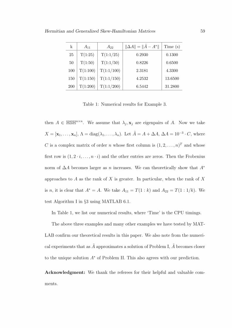
Hermitian and Generalized Skew-Hamiltonian Matrices 59
k A11 A22 ‖∆A‖ = ‖A−A∗‖ Time (s)
25 T(1:25) T(1:1/25) 0.2930 0.1300
50 T(1:50) T(1:1/50) 0.8226 0.6500
100 T(1:100) T(1:1/100) 2.3181 4.3300
150 T(1:150) T(1:1/150) 4.2532 13.6500
200 T(1:200) T(1:1/200) 6.5442 31.2800
Table 1: Numerical results for Example 3.
then A ∈ HSHn×n. We assume that λj,xj are eigenpairs of A. Now we take
X = [x1, . . . ,xn], Λ = diag(λ1, . . . , λn). Let A = A + ∆A, ∆A = 10−3 · C, where
C is a complex matrix of order n whose first column is (1, 2, . . . , n)T and whose
first row is (1, 2 · i, . . . , n · i) and the other entries are zeros. Then the Frobenius
norm of ∆A becomes larger as n increases. We can theoretically show that A∗
approaches to A as the rank of X is greater. In particular, when the rank of X
is n, it is clear that A∗ = A. We take A11 = T (1 : k) and A22 = T (1 : 1/k). We
test Algorithm I in §3 using MATLAB 6.1.
In Table 1, we list our numerical results, where ‘Time’ is the CPU timings.
The above three examples and many other examples we have tested by MAT-
LAB confirm our theoretical results in this paper. We also note from the numeri-
cal experiments that as A approximates a solution of Problem I, A becomes closer
to the unique solution A∗ of Problem II. This also agrees with our prediction.
Acknowledgment: We thank the referees for their helpful and valuable com-
ments.
Hermitian and Generalized Skew-Hamiltonian Matrices 60
References
[1] Z. Bai and R. Chan, Inverse Eigenproblem for Centrosymmetric and Cen-
troskew Matrices and Their Approximation, to appear in Theoretical Com-
puter Science.
[2] M. Baruch, Optimization Procedure to Correct Stiffness and Flexibility Ma-
trices Using Vibration Tests, AIAA J., 16 (1978), 1208–1210.
[3] A. Berman and E. Nagy, Improvement of Large Analytical Model Using Test
Data, AIAA J., 21 (1983), 1168–1173.
[4] X. Chen, Theoretical Methods and Its Application of Designing of Structured
Dynamics in Machine, The Mechanical Industry Press (in Chinese), Beijing,
1997, 165–202.
[5] E. Cheney, Introduction to Approximation Theory, McGraw-Hill, 1966.
[6] K. Chu and N. Li, Designing the Hopfield Neural Network via Pole Assign-
ment, Int. J. Syst. Sci., 25 (1994) 669–681.
[7] M. Chu and G. Golub, Structured Inverse Eigenvalue Problems, Acta Nu-
mer., 11 (2002) 1–71.
[8] K. Fan and A. Hoffman, Some Metric Inequalities in the Space of Matrices,
Proc. Amer. Math. Soc., 6 (1955), 111–116.
Hermitian and Generalized Skew-Hamiltonian Matrices 61
[9] X. Hu, L. Zhang, and D. Xie, The Solvability Conditions for the Inverse
Eigenvalue Problem of Bisymmetric Matrices, Math. Numer. Sin., 20 (1998),
409–418.
[10] K. Joseph, Inverse Eigenvalue Problem in Structural Design, AIAA J., 10
(1992), 2890–2896.
[11] A. Laub, Invariant Subspace Methods for the Numerical Solution of Riccati
Equations, in The Riccati Equation, S. Bittanti, A. Laub, and J. Willems,
eds., Springer-Verlag, Berlin, 1991, 163–196.
[12] N. Li, A Matrix Inverse Eigenvalue Problem and Its Application, Linear
Algebra Appl., 266 (1997) 143–152.
[13] V. Mehrmann, The Autonomous Linear Quadratic Control Problem, The-
ory and Numerical Solution, Lecture Notes in Control and Inform. Sci. 163,
Springer-Verlag, Heidelberg, 1991.
[14] T. Meng, Experimental Design and Decision Support, in Expert Systems,
The Technology of Knowledge Management and Decision Making for the
21st Century, Vol 1, ed. C. Leondes, Academic Press, 2001.
[15] S. Mitra, A Pair of Simultaneous Linear Matrix Equations A1XB1 = C1,
A2XB2 = C2 and a Matrix Programming Problem, Linear Algebra Appl.,
131 (1990), 107–123.
Hermitian and Generalized Skew-Hamiltonian Matrices 62
[16] Y. Sheng and D. Xie, The Solvability Conditions for the Inverse Problem
of Anti-Bisymmetric Matrices (in Chinese), J. Numer. Methods Comput.
Appl., 23 (2002), 111–120.
[17] V. Sima, Algorithms for Linear-Quadratic Optimization, Pure Appl. Math.,
200, Marcel Dekker, New York, 1996.
[18] J. Sun, Two Kinds of Inverse Eigenvalue Problems for Real Symmetric Ma-
trices, Math. Numer. Sin., 3 (1988), 282–290.
[19] J. Sun, Backward Perturbation Analysis of Certain Characteristic Subspaces,
Numer. Math., 65 (1993), 357–382.
[20] D. Xie, X. Hu, and L. Zhang, The Solvability Conditions for Inverse Eigen-
problem of Symmetric and Anti-Persymmetric Matrices and Its Approxima-
tion, Numer. Linear Algebra Appl., 10 (2003) 223–234.
[21] D. Xie and Y. Sheng, Inverse Eigenproblem of Anti-Symmetric and Per-
symmetric Matrices and Its Approximation, Inverse Problems, 19 (2003),
217–225.
[22] S. Xu, An Introduction to Inverse Algebraic Eigenvalue Problems, Peking
University Press and Vieweg Publishing, 1998.
[23] Z. Zhang, X. Hu, and L. Zhang, The Solvability Conditions for the Inverse
Eigenproblem of Hermitian-Generalized Hamiltonian Matrices, Inverse Prob-
lems, 18 (2002), 1369–1376.

Hermitian and Generalized Skew-Hamiltonian Matrices 63
[24] K. Zhou, J. Doyle, and K. Glover, Robust and Optimal Control, Prentice-
Hall, Upper Saddle River, NJ, 1995.
Inverse Eigenproblems for Centrosymmetric and
Centroskew Matrices and Their Approximation
Abstract
In this paper, we first give the solvability condition for the following
inverse eigenproblem (IEP): given a set of vectors {xi}mi=1 in Cn and a set of
complex numbers {λi}mi=1, find a centrosymmetric or centroskew matrix C
in Rn×n such that {xi}mi=1 and {λi}m
i=1 are the eigenvectors and eigenvalues
of C respectively. We then consider the best approximation problem for
the IEPs that are solvable. More precisely, given an arbitrary matrix B
in Rn×n, we find the matrix C which is the solution to the IEP and is
closest to B in the Frobenius norm. We show that the best approximation
is unique and derive an expression for it.
1 Introduction
Let Jn be the n-by-n anti-identity matrix, i.e, Jn has 1 on the anti-diagonal and
zeros elsewhere. An n-by-n matrix C is said to be centrosymmetric (or persym-
metric) if C = JnCJn, and it is called centroskew (or skew-centrosymmetric) if
C = −JnCJn. The centrosymmetric and centroskew matrices play an important
role in many areas [7, 16] such as signal processing [8, 11], the numerical solution
of differential equations [2], and Markov processes [17].
64
Centrosymmetric and Centroskew Matrices 65
In this paper, we consider two problems related to centrosymmetric and cen-
troskew matrices. Both problems are on numerical and approximate computing
but here we solve them algebraically, based on some explicit expressions for the
solutions of overdetermined linear systems of equations. The first problem is an
inverse eigenproblem. There are many applications of structured inverse eigen-
problems, see for instance the expository paper [5]. In particular, the inverse
eigenproblem for Toeplitz matrices (a special case of centrosymmetric matrices)
arises in trigonometric moment problem [10] and signal processing [9]. The in-
verse eigenproblem for centrosymmetric Jacobi matrices also comes from inverse
Sturm-Liouville problem [19, p.70]. There are also different types of inverse eigen-
problem, for instances multiplicative type and additive type [19, Chapter 4]. Here
we consider the following type of inverse eigenproblem which appeared in the de-
sign of Hopfield neural networks [4, 13].
Problem I. Given X = [x1,x2, . . . ,xm] in Cn×m and Λ = diag(λ1, . . . , λm)
in Cm×m, find a centrosymmetric or centroskew matrix C in Rn×n such that
CX = XΛ.
The second problem we consider in this paper is the problem of best approx-
imation:
Problem II. Let LS be the solution set of Problem I. Given a matrix B ∈ Rn×n,
Centrosymmetric and Centroskew Matrices 66
find C∗ ∈ LS such that
‖B − C∗‖ = minC∈LS
‖B − C‖,
where ‖ · ‖ is the Frobenius norm.
The best approximation problem occurs frequently in experimental design,
see for instance [14, p.123]. Here the matrix B may be a matrix obtained from
experiments, but it may not satisfy the structural requirement (centrosymmetric
or centroskew) and/or spectral requirement (having eigenpairs X and Λ). The
best estimate C∗ is the matrix that satisfies both requirements and is the best
approximation of B in the Frobenius norm. In addition, because there are fast
algorithms for solving various kinds of centrosymmetric and centroskew matrices
[12], the best approximate C∗ of B can also be used as a preconditioner in the pre-
conditioned conjugate gradient method for solving linear systems with coefficient
matrix B, see for instance [1].
Problems I and II have been solved for different classes of structured matrices,
see for instance [18, 20]. In this paper, we extend the results in [18, 20] to the
classes of centrosymmetric and centroskew matrices. We first give a solvability
condition for Problem I and also the form of its general solution. Then in the
case when Problem I is solvable, we show that Problem II has a unique solution
and we give a formula for the minimizer C∗.
The paper is organized as follows: In §2 we first characterize the class of
centrosymmetric matrices and give the solvability condition of Problem I over
Centrosymmetric and Centroskew Matrices 67
this class of matrices. In §3, we derive a formula for the best approximation of
Problem II, give the algorithm for finding the minimizer, and study the stability
of the problem. In §4 we give an example to illustrate the theory. In the last
section, we extend the results in §§2–3 to centroskew matrices.
2 Solvability Condition for Problem I
We first characterize the set of all centrosymmetric matrices. For all positive
integers k, let
K2k =1√2
Ik Ik
Jk −Jk
and K2k+1 =
1√2
Ik 0 Ik
0√
2 0
Jk 0 −Jk
.
Clearly Kn is orthogonal for all n. The matrix Kn plays an important role
in analyzing the properties of centrosymmetric matrices, see for example [6].
In particular, we have the following splitting of centrosymmetric matrices into
smaller submatrices using Kn.
Lemma 1 [6] Let Cn be the set of all centrosymmetric matrices in Rn×n. We
have
C2k =
E FJk
JkF JkEJk
∣∣ E, F ∈ Rk×k
},
C2k+1 =
E a FJk
bT c bT Jk
JkF Jka JkEJk
∣∣ E, F ∈ Rk×k, a,b ∈ Rk, c ∈ R
.
Centrosymmetric and Centroskew Matrices 68
Moreover, for all n = 2k and 2k + 1, we have
Cn =
Kn
G1 0
0 G2
KT
n
∣∣ G1 ∈ R(n−k)×(n−k), G2 ∈ Rk×k}
. (1)
Before we come to Problem I, we first note that we can assume without loss of
generality that X and Λ are real matrices. In fact, since Cn ⊂ Rn×n, the complex
eigenvectors and eigenvalues of any C ∈ Cn will appear in complex conjugate pairs.
If α±β√−1 and x±√−1y are one of its eigenpair, then we have Cx = αx−βy
and Cy = αy + βx, i.e.
C[x,y] = [x,y]
α β
−β α
.
Hence we can assume without loss of generality that X ∈ Rn×m and
Λ = diag(Φ1, Φ2, . . . , Φl, γ1, . . . , γm−2l) ∈ Rm×m, (2)
where Φi =
αi βi
−βi αi
with αi, βi and γi in R.
Next, we investigate the solvability of Problem I. We need the following lemma
where U+ denotes the Moore-Penrose pseudo-inverse of U .
Lemma 2 [15, Lemma 1.3] Let U, V ∈ Rn×m be given. Then Y U = V is
solvable if and only if V U+U = V . In this case the general solution is
Y = V U+ + Z(I − UU+),
where Z ∈ Rn×n is arbitrary.
In the remaining part of the paper, we will only give the theorems and the
proofs for even n. The case where n is odd can be proved similarly. Thus we let
n = 2k.
Centrosymmetric and Centroskew Matrices 69
Theorem 1 Given X ∈ Rn×m and Λ as in (2), let
KTn X =
X1
X2
, (3)
where X2 ∈ Rk×m. Then there exists a matrix C ∈ Cn such that CX = XΛ if
and only if
X1ΛX+1 X1 = X1Λ and X2ΛX+
2 X2 = X2Λ. (4)
In this case, the general solution to CX = XΛ is given by
Cs = C0 + Kn
Z1(In−k − X1X
+1 ) 0
0 Z2(Ik − X2X+2 )
KT
n , (5)
where Z1 ∈ R(n−k)×(n−k) and Z2 ∈ Rk×k are both arbitrary, and
C0 = Kn
X1ΛX+
1 0
0 X2ΛX+2
KT
n . (6)
Proof: From (1), C ∈ Cn is a solution to Problem I if and only if there exist
G1 ∈ R(n−k)×(n−k) and G2 ∈ Rk×k such that
C = Kn
G1 0
0 G2
KT
n (7)
and Kn
G1 0
0 G2
KT
n
X = XΛ. (8)
Using (3), (8) is equivalent to
G1X1 = X1Λ and G2X2 = X2Λ. (9)
Centrosymmetric and Centroskew Matrices 70
According to Lemma 2, equations (9) have solutions if and only if equations (4)
hold. Moreover in this case, the general solution of (9) is given by
G1 = X1ΛX+1 + Z1(In−k − X1X
+1 ), (10)
G2 = X2ΛX+2 + Z2(Ik − X2X
+2 ), (11)
where Z1 ∈ R(n−k)×(n−k) and Z2 ∈ Rk×k are both arbitrary. Putting (10) and
(11) into (7), we get (5).
3 The Minimizer of Problem II
Let CSn be the solution set of Problem I over Cn. In this section, we solve Problem
II over CSn when CS
n is nonempty.
Theorem 2 Given X ∈ Rn×m and Λ as in (2), let the solution set CSn of Problem
I be nonempty. Then for any B ∈ Rn×n, the problem minC∈CS
n
‖B − C‖ has a unique
solution C∗ given by
C∗ = C0 + Kn
B11(In−k − X1X
+1 ) 0
0 B22(Ik − X2X+2 )
KT
n . (12)
Here X1, X2, and C0 are given in (3) and (6), and B11 and B22 are obtained by
partitioning KTn BKn as
KTn BKn =
B11 B12
B21 B22
, (13)
where B22 ∈ Rk×k.
Proof: When CSn is nonempty, it is easy to verify from (5) that CS
n is a closed
convex set. Since Rn×n is a uniformly convex Banach space under the Frobenius
Centrosymmetric and Centroskew Matrices 71
norm, there exists a unique solution for Problem II [3, p. 22]. Moreover, because
the Frobenius norm is unitary invariant, Problem II is equivalent to
minC∈CS
n
‖KTn BK −KT
n CK‖2. (14)
By (5), we have
‖KTn BK −KT
n CK‖2 =
∥∥∥∥∥∥
B11 − X1ΛX+
1 B12
B21 B22 − X2ΛX+2
−
Z1P 0
0 Z2Q
∥∥∥∥∥∥
2
,
where
P = In−k − X1X+1 and Q = Ik − X2X
+2 . (15)
Thus (14) is equivalent to
minZ1∈R(n−k)×(n−k)
‖B11 − X1ΛX+1 − Z1P‖2 + min
Z2∈Rk×k‖B22 − X2ΛX+
2 − Z2Q‖2.
Clearly, the solution is given by Z1 and Z2 such that
Z1P = B11 − X1ΛX+1 and Z2Q = B22 − X2ΛX+
2 .
Notice that by (15), P and Q are projection matrices, i.e. P 2 = P and Q2 = Q.
Therefore Z1P = (B11− X1ΛX+1 )P and Z2Q = (B22− X2ΛX+
2 )Q. Notice further
that because X+1 X1X
+1 = X+
1 , we have
(B11 − X1ΛX+1 )P = B11 − B11X1X
+1 − X1ΛX+
1 + X1ΛX+1 X1X
+1
= B11 − B11X1X+1 = B11P.
Centrosymmetric and Centroskew Matrices 72
Similarly, Z2Q = (B22 − X2ΛX+2 )Q = B22Q. Hence the unique solution for
Problem II is given by (12).
Based on Theorem 2, we give the following algorithm for solving Problem II
for n = 2k.
ALGORITHM I
(a) Compute X1 and X2 by (3) and then compute X+1 and X+
2 .
(b) If X1ΛX+1 X1 = X1Λ and X2ΛX+
2 X2 = X2Λ, then the solution set CSn to
Problem I is nonempty and we continue. Otherwise we stop.
(c) Partition KTn BKn as in (13) to get B11 and B22.
(d) Compute
W1 = X1ΛX+1 + B11 − B11X1X
+1 ,
W2 = X2ΛX+2 + B22 − B22X2X
+2 .
(e) Then C∗ = Kn
W1 0
0 W2
KT
n .
Next we consider the computational complexity of our algorithm. For Step
(a), since Kn has only 2 nonzero entries per row, it requires O(nm) operations to
compute X1 and X2. Then using singular value decomposition to compute X+1
and X+2 requires O(n2m + m3) operations. Step (b) obviously requires O(n2m)
operations. For Step (c), because of the sparsity of Kn, the operations required is
Centrosymmetric and Centroskew Matrices 73
O(n2) only. For Step (d), if we compute BiiXiX+i as [(BiiXi)X
+i ], then the cost
will only be of O(n2m) operations. Finally, because of the sparsity of Kn again,
Step (e) requires O(n2) operations. Thus the total complexity of the algorithm
is O(n2m + m3). We remark that in practice, m ¿ n.
Before we end this section, we give a stability analysis for Problem II, that is,
we study how the solution of Problem II is affected by a small perturbation of B.
We have the following result.
Corollary 1 Given B(i) ∈ Rn×n, i = 1, 2. Let C∗(i) = arg minC∈CS
n
‖B(i) − C‖ for
i = 1, 2. Then there exists a constant α independent of B(i), i = 1, 2, such that
‖C∗(2) − C∗(1)‖ ≤ α‖B(2) −B(1)‖. (16)
Proof: By Theorem 2, C∗(i) is given by
C∗(i) = C0 + Kn
B(i)11 P 0
0 B(i)22 Q
KT
n , i = 1, 2,
where B(i)22 are the blocks of KT
n B(i)Kn as defined in (13), and P and Q are given
in (15). Thus we have
‖C∗(2) − C∗(1)‖ =
∥∥∥∥∥∥∥∥Kn
(B
(2)11 − B
(1)11
)P 0
0(B
(2)22 − B
(1)22
)Q
KT
n
∥∥∥∥∥∥∥∥
≤
∥∥∥∥∥∥∥∥
B(2)11 − B
(1)11 0
0 B(2)22 − B
(1)22
∥∥∥∥∥∥∥∥
∥∥∥∥∥∥∥∥
P 0
0 Q
∥∥∥∥∥∥∥∥
≤∥∥KT
n
(B(2) −B(1)
)Kn
∥∥
∥∥∥∥∥∥∥∥
P 0
0 Q
∥∥∥∥∥∥∥∥≤ α
∥∥B(2) −B(1)∥∥ ,
Centrosymmetric and Centroskew Matrices 74
where α = ‖P‖+ ‖Q‖. Thus (16) holds.
4 Demonstration by an Example
Let us first compute the input matrices X and Λ for which Problem I has a
solution. We start by choosing a random matrix C in Cn:
C =
0.1749 0.0325 −0.2046 0.0932 0.0315
0.0133 −0.0794 −0.0644 0.1165 −0.0527
0.1741 0.0487 0.1049 0.0487 0.1741
−0.0527 0.1165 −0.0644 −0.0794 0.0133
0.0315 0.0932 −0.2046 0.0325 0.1749
∈ C5.
Then we compute its eigenpairs. The eigenvalues of C are 0.1590± 0.2841√−1,
−0.1836, 0.1312, and 0.0304. Let x1±√−1x2, x3,x4, and x5 be the corresponding
eigenvectors. Then we take
X = [x1,x2,x3,x4,x5] =
0.4815 0.2256 −0.2455 −0.7071 −0.1313
0.0118 0.1700 0.7071 −0.1427 −0.7071
0.4322 −0.5120 0.2235 0 0
0.0118 0.1700 0.7071 0.1427 0.7071
0.4815 0.2256 −0.2455 0.7071 0.1313
Centrosymmetric and Centroskew Matrices 75
and
Λ =
0.1590 0.2841 0 0 0
−0.2841 0.1590 0 0 0
0 0 0.0304 0 0
0 0 0 0.1312 0
0 0 0 0 −0.1836
.
Given this X and Λ, clearly we have a solution to Problem I, namely C. Thus
CS5 is nonempty. Next we perturb C by a random matrix to obtain a matrix
B(ε) 6∈ C5:
B(ε) = C + ε ·
1.4886 −0.9173 1.2688 −0.1869 −1.0830
1.2705 −1.1061 −0.7836 1.0132 1.0354
−1.8561 0.8106 0.2133 0.2484 1.5854
2.1343 0.6985 0.7879 0.0596 0.9157
1.4358 −0.4016 0.8967 1.3766 −0.5565
.
Then we can apply our algorithm in §3 to obtain C∗(ε) corresponding to B(ε).
In Figure 1, we plot the following two quantities for ε between 10−10 to 1010:
log10 ‖B(ε) − C∗(ε)‖ (marked by “∗”) and log10 ‖C − C∗(ε)‖ (marked by “+”).
We can see that as ε goes to zero, C∗(ε) approaches B(ε) as expected. Also when
ε ≤ 10−1, C∗(ε) = C up to the machine precision (we use matlab which has
machine precision around 10−16).
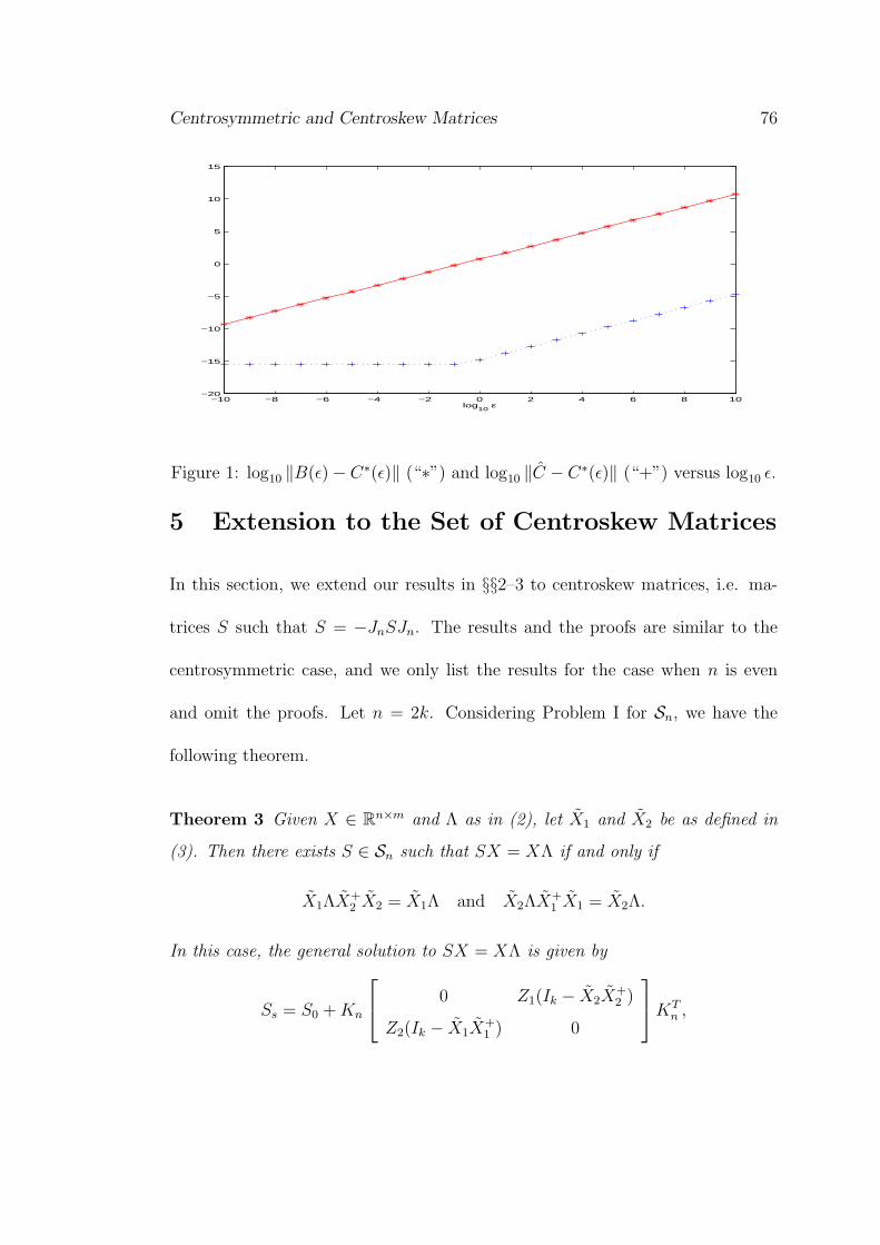
Centrosymmetric and Centroskew Matrices 76
−10 −8 −6 −4 −2 0 2 4 6 8 10−20
−15
−10
−5
0
5
10
15
log10
ε
Figure 1: log10 ‖B(ε)− C∗(ε)‖ (“∗”) and log10 ‖C − C∗(ε)‖ (“+”) versus log10 ε.
5 Extension to the Set of Centroskew Matrices
In this section, we extend our results in §§2–3 to centroskew matrices, i.e. ma-
trices S such that S = −JnSJn. The results and the proofs are similar to the
centrosymmetric case, and we only list the results for the case when n is even
and omit the proofs. Let n = 2k. Considering Problem I for Sn, we have the
following theorem.
Theorem 3 Given X ∈ Rn×m and Λ as in (2), let X1 and X2 be as defined in
(3). Then there exists S ∈ Sn such that SX = XΛ if and only if
X1ΛX+2 X2 = X1Λ and X2ΛX+
1 X1 = X2Λ.
In this case, the general solution to SX = XΛ is given by
Ss = S0 + Kn
0 Z1(Ik − X2X
+2 )
Z2(Ik − X1X+1 ) 0
KT
n ,
Centrosymmetric and Centroskew Matrices 77
where Z1 ∈ Rk×k and Z2 ∈ Rk×k are both arbitrary, and
S0 = Kn
0 X1ΛX+
2
X2ΛX+1 0
KT
n . (17)
For Problem II over the solution set SSn of Problem I for Sn, we have the
following result.
Theorem 4 Given X ∈ Rn×m and Λ as in (2), let the solution set SSn of Problem
I be nonempty. Then for any B ∈ Rn×n, the problem minS∈SS
n
‖B − S‖ has a unique
solution S∗ given by
S∗ = S0 + Kn
0 B12(Ik − X2X
+2 )
B21(In−k − X1X+1 ) 0
KT
n .
Here X1, X2, B12, B21, and S0 are given in (3), (13), and (17). Moreover S∗ is
a continuous function of B.
Acknowledgments:
We thank the referees for their helpful and valuable comments.
References
[1] T. Chan, An Optimal Circulant Preconditioner for Toeplitz Systems, SIAM J.
Sci. Stat. Comput., 9 (1988), 766–771.
[2] W. Chen, X. Wang, and T. Zhong, The Structure of Weighting Coefficient
Matrices of Harmonic Differential Quadrature and Its Application, Comm.
Numer. Methods Engrg., 12 (1996), 455–460.
[3] E. Cheney, Introduction to Approximation Theory, McGraw-Hill, 1966.
Centrosymmetric and Centroskew Matrices 78
[4] K. Chu and N. Li, Designing the Hopfield Neural Network via Pole Assign-
ment, Int. J. Syst. Sci., 25 (1994), 669–681.
[5] M. Chu and G. Golub, Structured Inverse Eigenvalue Problems, Acta Numer.,
11 (2002), 1–71.
[6] A. Collar, On Centrosymmetric and Centroskew Matrices, Quart. J. Mech.
Appl. Math., 15 (1962), 265–281.
[7] L. Datta and S. Morgera, On the Reducibility of Centrosymmetric Matrices
– Applications in Engineering Problems, Circuits Systems Signal Process., 8
(1989), 71–96.
[8] J. Delmas, On Adaptive EVD Asymptotic Distribution of Centro-symmetric
Covariance Matrices, IEEE Trans. Signal Process., 47 (1999), 1402–1406.
[9] G. Feyh and C. Mullis, Inverse Eigenvalue Problem for Real Symmetric
Toeplitz Matrices, International Conference on Acoustics, Speech, and Sig-
nal Processing, 3 (1988), 1636–1639.
[10] U. Grenander and G. Szego, Toeplitz Forms and Their Applications, Chelsea
Publishing Company, New York, 1984.
[11] N. Griswold and J. Davila, Fast Algorithm for Least Squares 2D Linear-Phase
FIR Filter Design, IEEE International Conference on Acoustics, Speech, and
Signal Processing, 6 (2001), 3809–3812.
Centrosymmetric and Centroskew Matrices 79
[12] T. Kailath and A. Sayed, Fast Reliable Algorithms for Matrices with Struc-
tures, SIAM, 1999.
[13] N. Li, A Matrix Inverse Eigenvalue Problem and Its Application, Linear
Algebra Appl., 266 (1997), 143–152.
[14] T. Meng, Experimental Design and Decision Support, in Expert Systems,
The Technology of Knowledge Management and Decision Making for the 21st
Century, Vol 1, ed. C. Leondes, Academic Press, 2001.
[15] J. Sun, Backward Perturbation Analysis of Certain Characteristic Subspaces,
Numer. Math., 65 (1993), 357–382.
[16] D. Tao and M. Yasuda, A Spectral Characterization of Generalized
Real Symmetric Centrosymmetric and Generalized Real Symmetric Skew-
Centrosymmetric Matrices, SIAM J. Matrix Anal. Appl., 23 (2002), 885–895.
[17] J. Weaver, Centrosymmetric (Cross-symmetric) Matrices, Their Basic Prop-
erties, Eigenvalues, and Eigenvectors, Amer. Math. Monthly, 92 (1985), 711–
717.
[18] D. Xie, X. Hu, and L. Zhang, The Solvability Conditions for Inverse Eigen-
problem of Symmetric and Anti-persymmetric Matrices and Its Approxima-
tion, Numer. Linear Algebra Appl., to appear.
[19] S. Xu, An Introduction to Inverse Algebraic Eigenvalue Problems, Peking
University Press and Vieweg Publishing, 1998.

Centrosymmetric and Centroskew Matrices 80
[20] L. Zhang, D. Xie, and X. Hu, The Inverse Eigenvalue Problems of Bisymmet-
ric Matrices on the Linear Manifold, Math. Numer. Sin., 22 (2000), 129–138.