Embed Size (px)
Citation preview

ORE Open Research Exeter
TITLE
Numerical model validation for mooring systems: Method and application for wave energyconverters
AUTHORS
Harnois, Violette; Weller, S.D.; Johanning, Lars; et al.
JOURNAL
Renewable Energy
DEPOSITED IN ORE
20 November 2014
This version available at
http://hdl.handle.net/10871/15903
COPYRIGHT AND REUSE
Open Research Exeter makes this work available in accordance with publisher policies.
A NOTE ON VERSIONS
The version presented here may differ from the published version. If citing, you are advised to consult the published version for pagination, volume/issue and date ofpublication

Numerical model validation for mooring systems: Method and 1
application for wave energy converters 2
Harnois, V.a, Weller, S.D.
a, Johanning, L.
a, Thies, P.R.
a, Le Boulluec, M.
b, Le Roux, D.
b, Soulé, V.
b, Ohana J.
b 3
4
a [email protected] (Corresponding author) 5
+0044 (0)1326 259308 6
[email protected], [email protected], [email protected] 7
College of Engineering, Mathematics and Physical Sciences 8
University of Exeter, Cornwall Campus, Cottage 2 9
Penryn, Cornwall TR10 9FE, UK 10
11
b [email protected] , [email protected] , [email protected] 12
IFREMER 13
Hydrodynamique & Océano-Météo 14
BP 70 – 29280 Plouzané – France 15
16

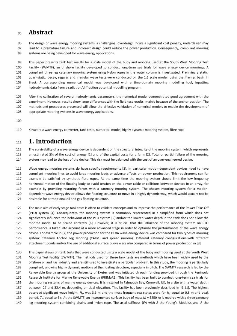
Fig. 1 Wave basin installation and numerical model settings: a) side view of the buoy and dimensions, b) top view of the 17
truncated mooring and of the wave gauge layout, c) photograph of the SWMTF model in the basin, with the false floor and 18
d) buoy hull mesh used for the radiation/diffraction potential analysis 19
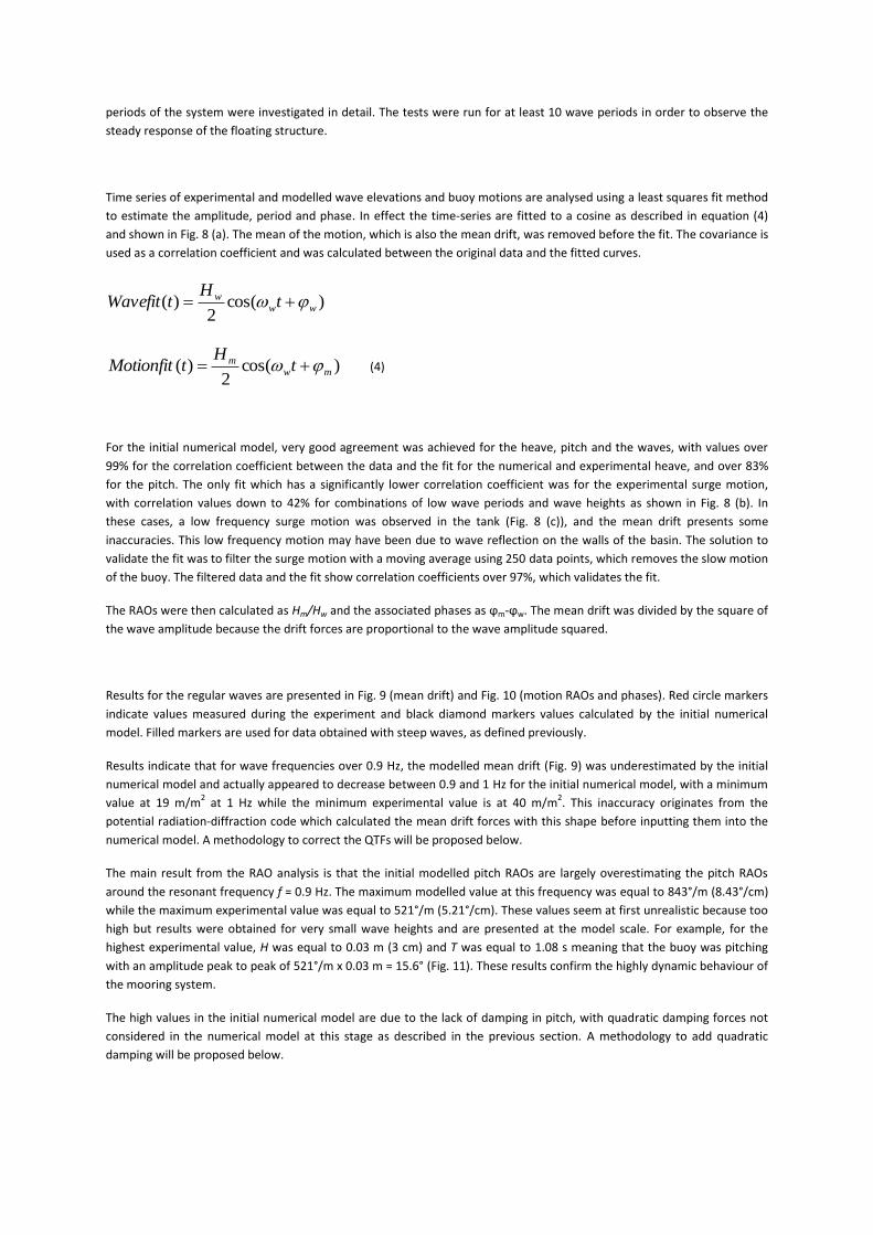
Fig. 2 Range of tests needed to validate a numerical model with experimental data 20
Fig. 3 Mooring stiffness: a) comparison of the experimental (red circles and solid line) and modelled (blue circles and 21
dashed line) mooring load/buoy surge offset relationship and b) relative error in mooring tension between experimental 22
and modelled values 23
Fig. 4 Example of calculation of the natural period and linear and quadratic damping: a) detection of peaks and troughs and 24
calculation of the natural period, b) calculation of the linear p1 and quadratic p2 damping coefficients using a linear fit; 25
norm of the residua l= 0.036 26
Fig. 5 Time-series of decay tests in a) surge, with comparison between the experimental values (red solid line), initial 27
(dashed black line) and corrected numerical model (blue dotted line) and in b) pitch, with a plot of the experimental surge 28
motion to show the coupling between surge and pitch 29
Fig. 6 Sensitivity analysis for the surge decay: a) for the added mass; b) for the quadratic damping; c) for the linear damping 30
Fig. 7 Review of tests in regular waves: a) Wave heights, H, and wave periods, T, used for the tank tests. b) Selection of 31
steep waves, the green line is for D
KC
14.0
2
1 , separating the steep and the linear waves, and the blue line for 32
DKC
14.0 , separating steep waves and breaking waves. The black filled circles indicate steep waves while the red 33
hollow circles indicate linear waves 34
Fig. 8 Examples of fit of the experimental surge motion: a) for H = 0.1 m and T = 1.7 s (blue line: signal, black line: fit); b) 35
Summary of the correlation coefficient between the fit and the experimental values c) Examples of fit for H = 0.05 m and T 36
= 0.9 s where a low frequency motion on the X axis can be observed (blue line: signal, black line: fit) 37
Fig. 9 Mean drift divided by the square of the wave amplitude for different wave frequencies and wave steepness values. 38
Fig. 10 Motion RAOs for the surge, heave and pitch (from top to bottom): amplitudes (left) and phases (right) 39
Fig. 11 Regular wave tank test with the highest pitch RAO (H = 0.03 m and T = 1.08 s). a) Time series of the surface 40
elevation and pitch motion b) Picture of the buoy at its maximum pitch RAO 41
Fig. 12 Sensitivity analysis for the surge mean drift forces for the linear waves a) calculation of the mean drift for all sea 42
states with the mean drift forces multiplied by different coefficients b) for a given sea state, calculation of the corrective 43
mean drift force multiplicative factor which leads to equal experimental and numerical mean drift (here for H = 0.6 m and T 44
= 1.9 s); c) for frequencies over 0.85 Hz, fit of the corrective multiplicative factors; d) Corrected mean drift forces and 45
smoothing of the values 46
Fig. 13 Sensitivity analysis for the pitch additional quadratic damping: a) calculation of pitch RAO for different values of 47
additional quadratic damping for all sea states. QD stands for additional quadratic damping; b) minimisation of the sum of 48
the absolute value of the difference between experimental and numerical pitch RAOs 49
Fig. 14 Example of wave inputs for Case 2. The red dots are the signal measured during the experiment and the blue dots 50
are for the corrected signal used as an input in the numerical model with different sampling frequencies: a) 100 Hz, b) 10 51
Hz, c) 4 Hz 52
Fig. 15 Example of motion time series for Case 2: a) surge motion, b) heave motion and c) pitch motion. Red line: 53
experiment, thick blue line: numerical model 54
Fig. 16 Example of mooring load time series for Case 2: a) in the front line 1, b) in the back line 2, c) in the other front line 3. 55
Red line: experiment, thick blue line: numerical model 56

Fig. 17 Example of mooring load time series for Case 2 using different parameters for the numerical model: a) surge 57
motion, b) heave motion, c) pitch motion, d) in the front line 1, e) in the back line 2, f) in the other front line 3. Solid red 58
line: experiment, blue dashed line: numerical model with full QTFs, black dotted line: numerical model using Newman’s 59
approximation with diagonal corrections 60
Fig. 18 Example of time series for Case 1 of mooring loads (a-c), motion (d-e) and waves (f) for the experiment in the tank 61
(red thick) and the experiment in the field (blue dots). Results are shown at model scale. Red line: laboratory experiment, 62
thick blue line: field tests 63
Fig. 19 Variations in motions and loads for Case 2 with models using different rope stiffness: a) Normalised correlation 64
coefficient between the model with a given stiffness and the model used in this study; b) Normalised maximum mooring 65
load with the models using different stiffness 66
67
68
69
Table 1 Properties of the original mooring lines and of the simplified, scaled and truncated mooring lines where Cdn and 70
Cmn are normal drag and inertia coefficients, Cda and Cma are axial drag and inertia coefficients, T = tonnes 71
Table 2 Full scale and model buoy properties and difference with theoretical values where COG = centre of gravity 72
Table 3 Results for the surge decay tests: amplitude of release and after one oscillation, natural period Tm, linear damping 73
p1 and quadratic damping p2, and norm of the residuals associated with the damping linear fit 74
Table 4 Results for the pitch decay tests: amplitude of release, natural period Tm, linear damping p1 and quadratic damping 75
p2, and norm of the residuals associated with the damping linear fit 76
Table 5 Comparison of experimental and numerical results: natural period Tm, linear damping p1 and quadratic damping p2 77
for surge decay 78
Table 6 Correction implemented on added mass, linear damping p1 and quadratic damping p2 for the surge motion 79
Table 7 Statistical properties of the irregular sea states as calculated by WavesMon, the ADCP firmware using the field 80
data, and plot of the field data spectrum with WAFO function dat2spec [20], using default frequency smoothing (parzen 81
window function on the estimated autocovariance function) 82
Table 8 Comparison of experimental measurements and numerical model results for the wave elevation, buoy motions and 83
mooring loads 84
Table 9 Comparison of maximum mooring loads for the different cases and the different mooring lines 85
Table 10 Comparison of correlation coefficients between the numerical model results using different sampling frequencies 86
for the wave input and the experimental results for the wave elevation, buoy motions and mooring loads for Case 1 87
Table 11 Comparison of correlation coefficients between the numerical model results using the Newman’s approximation 88
(before and after correction of the mean drift) and using the full QTFs for the buoy motions and mooring loads for Case 1 89
Table 12 Comparison of mean and standard deviations between the tank test results and the field test results for the wave 90
elevation, buoy motions and mooring loads. Results are given at the model scale. 91
92
93
94
Abstract 95
The design of wave energy mooring systems is challenging: overdesign incurs a significant cost penalty, underdesign may 96
lead to a premature failure and incorrect design could reduce the power production. Consequently, compliant mooring 97
systems are being developed for wave energy applications. 98
This paper presents tank test results for a scale model of the buoy and mooring used at the South West Mooring Test 99
Facility (SWMTF), an offshore facility developed to conduct long-term sea trials for wave energy device moorings. A 100
compliant three leg catenary mooring system using Nylon ropes in the water column is investigated. Preliminary static, 101
quasi-static, decay, regular and irregular wave tests were conducted on the 1:5 scale model, using the Ifremer basin in 102
Brest. A corresponding numerical model was developed with a time-domain mooring modelling tool, inputting 103
hydrodynamic data from a radiation/diffraction potential modelling program. 104
After the calibration of several hydrodynamic parameters, the numerical model demonstrated good agreement with the 105
experiment. However, results show large differences with the field test results, mainly because of the anchor position. The 106
methods and procedures presented will allow the effective validation of numerical models to enable the development of 107
appropriate mooring systems in wave energy applications. 108
109
Keywords: wave energy converter, tank tests, numerical model, highly dynamic mooring system, fibre rope 110
1. Introduction 111
The survivability of a wave energy device is dependent on the structural integrity of the mooring system, which represents 112
an estimated 5% of the cost of energy [1] and of the capital costs for a farm [2]. Total or partial failure of the mooring 113
system may lead to the loss of the device. This risk must be balanced with the cost of an over-engineered design. 114
Wave energy mooring systems do have specific requirements [3]. In particular motion-dependent devices need to have 115
compliant mooring lines to avoid large mooring loads or adverse effects on power production. This requirement can for 116
example be satisfied by synthetic fibre ropes. At the same time the mooring system should limit the low-frequency 117
horizontal motion of the floating body to avoid tension on the power cable or collisions between devices in an array, for 118
example by providing restoring forces with a catenary mooring system. The chosen mooring system for a motion-119
dependent wave energy device allows the floating structure to move in a highly dynamic way, which would usually not be 120
desirable for a traditional oil and gas floating structure. 121
The main aim of early stage tank tests is often to validate concepts and to improve the performance of the Power Take-Off 122
(PTO) system [4]. Consequently, the mooring system is commonly represented in a simplified form which does not 123
significantly influence the behaviour of the PTO system [5] and/or the limited water depth in the tank does not allow the 124
moored model to be scaled correctly [6]. However, it is crucial that the influence of the mooring system on PTO 125
performance is taken into account at a more advanced stage in order to optimise the performances of the wave energy 126
device. For example in [7] the power production for the DEXA wave energy device was compared for two types of mooring 127
system: Catenary Anchor Leg Mooring (CALM) and spread mooring. Different catenary configurations-with different 128
attachment points and/or the use of additional surface buoys were also compared in terms of power production in [8]. 129
This paper draws on tank tests that were conducted using a scale model of the buoy and mooring used at the South West 130
Mooring Test Facility (SWMTF). The methods used for these tank tests are methods which have been widely used by the 131
offshore oil and gas industry and are still used to investigate a particular problem. In this study, the mooring is particularly 132
compliant, allowing highly dynamic motions of the floating structure, especially in pitch. The SWMTF research is led by the 133
Renewable Energy group at the University of Exeter and was initiated through funding provided through the Peninsula 134
Research Institute for Marine Renewable Energy (PRIMaRE). This facility has been built to conduct long-term sea trials for 135
the mooring systems of marine energy devices. It is installed in Falmouth Bay, Cornwall, UK, in a site with a water depth 136
between 27 and 32.4 m, depending on tidal elevation. This facility has been previously described in [9-11]. The highest 137
observed significant wave height, HS, was 3.5 m and the most frequent sea states were for HS equal to 0.8 m and peak 138
period, TP, equal to 6 s. At the SWMTF, an instrumented surface buoy of mass M = 3250 kg is moored with a three catenary 139
leg mooring system combining chains and nylon rope. The axial stiffness (EA with E the Young’s Modulus and A the 140

sectional area of the rope) of dry nylon rope used as part of the SWMTF mooring system was measured from tension-141
tension tests conducted using the Dynamic Marine Component (DMaC) facility at the University of Exeter [12]. For a range 142
of harmonic loading regimes with mean loads and amplitudes not exceeding 1.0% and 0.6% respectively of the Minimum 143
Breaking Load (MBL), the rope sample demonstrated axial stiffness values between 889-972 kN for oscillation periods 144
ranging from 25 to 100 s. 145
This paper is divided in 5 sections, including the introduction. Section 2 will describe the experimental set-up and the 146
numerical modelling of the mooring system. Section 3 gives results from static and quasi-static tests, decay tests, as well as 147
regular and irregular wave tests. The results are discussed in section 4 followed by a conclusion in section 5. 148
149
2. Experimental set-up and modelling of the mooring system 150
This section describes the experimental set-up and the numerical modelling of the mooring system. The properties of the 151
basin and its instrumentation are described, the choice of scale is explained, and the scaled properties of the buoy and its 152
mooring are detailed. Finally, the inputs of the numerical model are defined. 153
2.1 Experimental set-up 154
The tank tests were performed in the Ifremer deep water wave basin in Brest, France. This tank uses sea water with a 155
density of 1.026 kg/m3
at 17.2°C, and 35.6% salinity (averages based on three sample measurements during the test period 156
using the method described by Sharqawy et al. [13]. The basin is 50 m long, 12.5 m wide and 10 m deep for the first three 157
quarters of its length, where the model is installed. The wave generator is able to generate waves with maximum 158
amplitude of 0.5 m and with periods from 0.8 to 3.5 s. The mooring loads were recorded with axial load cells installed on 159
the top of each mooring line. Six degree of freedom motions at the centre of gravity of the buoy were determined using a 160
Qualysis™ video motion tracking system with reflecting targets mounted on the top of the buoy (Fig. 1 (a)). Surface 161
elevations were measured with servo wave gauges, installed as shown in Fig. 1 (b). All measured signals were time 162
synchronised and recorded at 100 Hz. 163
164
The scale of the model was determined by the dimensions of the tank, particularly its width. An initial full-scale static 165
numerical investigation with Orcaflex™ was carried out to estimate the length of mooring line constantly resting on the 166
seabed for a range of surge/sway (+/-30 m) and heave (+/-15 m) buoy motions. These motions were the largest observed 167
motions during the sea trials of the SWMTF. The portion of mooring line which rests on the seabed during large 168
displacements does not significantly interfere with the hydrodynamic behaviour of the system and can therefore be 169
truncated. The results of this preliminary study indicated that a Froude model scale of 1:5 with a water depth of 5.95 m 170
was feasible. A false floor was installed in the tank to achieve the desired water depth (Fig. 1 (c)). Truncated mooring lines 171
were simplified and scaled (Table 1). For example, on the full scale SWMTF mooring, section 4 of the mooring line is made 172
of a DN24 openlink chain and of a 9.5 tonnes shackle. In the scale model mooring, only a chain was used while taking into 173
account the weight of the shackle. The drag and inertia coefficients for the mooring lines were taken from DNV standards 174
[14] for the nylon lines and from the Orcaflex™ manual [15] for the chains. The axial stiffness of three samples extracted 175
from the used model rope was quantified using tension testing equipment at Ifremer [16]. The yarns demonstrated axial 176
stiffness values between 10.0 and 12.6 kN when subjected to scaled (by N/Tex) loading using a 25 s oscillation period. An 177
average value of 10.873 kN was used in the numerical model, while the scaled value of the stiffness of the rope used at the 178
SWMTF ranges between 7.1 and 7.8 kN. 179
180
The model was orientated with mooring lines 1 and 3 facing the wave symmetrically (Fig. 1 (b)), and all tests were carried 181
out with a wave incidence angle equal to zero. Table 2, adapted from [17] gives details about the scale model properties, 182
and the differences between the theoretical scaled values and the measured scaled values. Fig. 1 (a) illustrates the 183
dimensions of the scaled buoy. 184
2.2 Modelling of the mooring system Mooring system software such as Orcaflex™ requires the specification of hydrodynamic parameters. Hydrostar™, a
radiation/diffraction potential code, was used to calculate the hydrodynamic properties for a simplified hull shape (Fig. 1

(d)) and for each wave frequency, from 0.11 to 13.42 rad/s, in increments of 0.11 rad/s. The mesh was calculated with
Matlab, includes 3145 points and 3024 faces, and is symmetrical with respect to the vertical axis. This simplified shape
does not include the vertical triangular braces at the bottom of the buoy (Fig. 1 (a)), therefore the added mass and
hydrodynamic damping associated with these features are not accounted for. The frequency-dependent data calculated
using this mesh for each of the 6 degrees of freedom of the buoy were:
a) the load Response Amplitude Operators (RAOs) and associated phases at the metacentre at the equilibrium position of
the buoy,
b) the added masses at the centre of gravity (COG) of the buoy,
c) the radiation damping values at the COG of the buoy, and
d) the Quadratic Transfer Functions (QTFs) at the metacentre at the equilibrium of the buoy.
The viscous damping cannot be calculated by radiation/diffraction potential codes.
To simplify the Orcaflex™ calculations, Newman’s approximation was used for the QTFs. This approximation considered
that the full QTFs should not influence significantly the behaviour of the device; consequently only the mean drift forces
are required to estimate the second order motion of the floating structure. Hauteclocque et al. [18] discussed the
differences in results using different methods to calculate the second-order low frequency loads in shallow water and
found that the two key parameters for a proper estimation of the behaviour of the moored system are the water depth
and the resonance period: the Newman approximation can give accurate results for a compliant system in deep water. For
this experiment, the low Ursell number (eq 1) [19] indicates that the conditions are linear (linear wave theory).
Furthermore, the mooring system is highly compliant, and its resonance frequencies, highlighted by the regular wave tests
are relatively small.
In order to validate this assumption, a model runs with the full QTFs will be compared with a model using the Newman’s
approximation in subsection 3.4.
100081.095.58
2.55.0
8 32
2
32
2
maxmaxmax
h
HUr (1)
where Hmax is the highest wave height used for regular wave tests, λmax is the highest wave length used for regular wave
tests and h is the water depth.
3. Validation results This section will present results from the different tests. The aim of this series of tests is to obtain an accurate model in
realistic sea states. As shown in Fig. 2, each test will provide different information about the hydrodynamics of the buoy
and its mooring. This information will then be used to finely calibrate the numerical model and correct potential
inaccuracies. The calibration of the model will be done using best fit models a) for the surge added mass, quadratic
damping and linear damping using the decay test results and b) for the pitch quadratic damping and surge QTFs using the
regular wave test results. The drag forces applied on the mooring lines are assumed to be correct.
The numerical model is build using the potential radiation-diffraction theory. Consequently, the buoy properties (RAOs,
added mass...) have been calculated for a constant draft and for infinitesimally small waves. As discussed previously, the
Newman’s approximation has been used for the QTFs to simplify the calculations.

3.1 Static and quasi static tests Static tests were conducted in still water conditions to determine the buoy draft, with and without mooring lines in place.
In free-floating conditions, before attaching the mooring lines, the centre of gravity of the buoy was at 0.078 m below the
mean water level in the basin. This distance was set in the numerical model. After the attachment of the mooring lines, the
centre of gravity was 0.10 m below the mean water level and the mooring pre-tension was 18 N in both the basin and the
numerical model.
Quasi-static tests were used to identify the horizontal stiffness characteristics of the mooring system, by determining the
relationship between the buoy horizontal position and the mooring line tensions. The model was placed in the basin in still
water conditions. The buoy was held in different surge positions and the mooring tensions were measured for each surge
position.
The results of the quasi-static tests are presented in Fig. 3 (a), indicating the tension in the mooring lines for a given surge
offset. The results of the tank tests and of the numerical model show an excellent agreement with a relative error not
exceeding 6% (Fig. 3 (b)).
3.2. Decay tests Decay tests were carried out to evaluate the linear and quadratic damping and the added mass of the buoy from its natural
period. Decay tests involved moving the moored buoy from its equilibrium position in one degree of freedom and then
releasing it. The buoy is moving at its natural frequency for this degree of freedom, and the amplitude of motion is
decreasing because of the damping of the system. A Matlab™ code called Wave Analysis for Fatigue and Oceanography,
usually referred to as WAFO [20], was used to detect peaks and troughs in the decay time series. The first decay oscillation
was ignored for calculation, because the buoy may have experienced additional damping due to the release of the
mooring. For each decay test, the subsequent 5 peaks and 5 troughs were used to calculate the natural period and
damping coefficients. The amplitude of release used for the numerical model was the mean amplitude after the first
oscillation during the tank tests. The amplitudes of release and after one oscillation during tank tests are given in Table 3
(surge) and Table 4 (pitch).
The natural period depends mainly on the stiffness of the moored system, its mass and added mass [21]. Quasi static tests
indicated that the stiffness of the mooring system in the numerical model is very close to the experimental stiffness, and
the model buoy was weighed before the tank tests, as shown in Table 2, with a perfect agreement between the
experimental and numerical values. By elimination of the other parameters, this means that the natural period will validate
the value of added mass calculated by the radiation-diffraction code. The natural period was calculated as the mean time
between similar extreme values (peak or trough).
The radiation damping forces depend linearly on the magnitude of relative velocity of the sea past the buoy, and the
viscous damping by a quadratic relationship. The overall damping was calculated for the tank tests and for the numerical
model, and was separated into a linear and a quadratic coefficient: iωξpp j21 , with jξ the motion amplitude in
one degree of freedom and ω the angular frequency. p1 and p2 are coefficients which can be calculated using the relation
described by Faltinsen [22], assuming the damping to be constant with respect to the oscillation amplitude:
21
1
1
3
16log
2p
T
Xp
X
X
T m
n
n
n
m
(2)
where Xn is the amplitude of the nth
oscillation and Tm is the natural period of oscillation. Fig. 4 (a) and (b) illustrate this
method: a) extremes are detected, and b)
1
1log2
n
n
m X
X
T is plotted against
m
n
T
X
3
16, allowing the calculation of p1 and
p2 by linear regression using a least squares method. The norm of the residual was calculated to give an indication of the
goodness of the fit.

Decay results from the tank tests and from the initial numerical model are presented in Fig. 5 (a) and (b) and Table 3-5.
Test repeatability was evaluated using the standard deviations of natural period, damping coefficients and norms of the
residuals between the different experiments. Table 3 indicates that for the different surge decay tests, similar results were
obtained for the natural period and the quadratic damping coefficients, and more variability was observed for the linear
damping coefficients. Because of this repeatability, the values chosen to calibrate the numerical model are the mean
values of natural period and damping coefficients over the six experiments. The pitch decay tests provide a larger range of
natural period and damping values for the different experiments. This lack of repeatability may be due to a coupling of the
pitch motion with the surge motion, as seen in Fig. 5 (b). In these cases, large amplitudes of the surge motion-up to 0.4m-
are observed and the pitch motion does not oscillate around zero. Because of this lack of repeatability, the pitch motion
properties could not be evaluated accurately and the experimental values could not be used to calibrate the numerical
model.
The initial numerical model was underestimating the damping of the system and the natural period in surge (Fig. 5 (a),
Table 5). The inaccuracies in the added mass and linear damping may have been due to the simplified shape or the
inabilities of the radiation-diffraction model to evaluate viscous damping. Following an iterative process, the added mass,
linear and quadratic damping values were adjusted until the numerical natural periods and damping coefficients matched
the experimental values:
a) The surge added mass is multiplied by coefficients between 1 and 1.5 for all the wave frequencies and simulations are
run with these corrected added masses; the natural period is calculated for each added mass simulation and plotted
against the multiplying coefficients (Fig. 6 (a)). A linear fit estimates the value of the multiplying coefficient which leads to a
similar experimental and modelled natural period.
b) Additional quadratic damping value is added to the numerical model with values between 0 and the total quadratic
damping value, p2, calculated from the tank tests. Simulations are run with this additional damping. The quadratic damping
coefficient, p2, is calculated for each simulation and plotted against the additional quadratic damping (Fig. 6 (b)). A linear fit
gives the value of additional damping which leads to a similar experimental and modelled quadratic damping, p2.
c) Additional linear damping is slowly increased in the numerical model. For each value of additional linear damping, the
linear damping coefficient, p1, is calculated and plotted against the value of additional linear damping (Fig. 6 (c)). Following
a similar method than previously, a value of additional linear damping is chosen for further calculations.
Calibrations are summarised in Table 6. For the surge, the corrected model shows a good agreement with the experimental
data, as seen in Fig. 5 (a) or Table 5, with less than 8% relative error between the measured and modelled natural periods
and damping values.
3.3. Regular waves tests Regular wave tests aim to evaluate Response Amplitude Operators (RAOs) of the buoy motions together with the mean
drift for a large range of wave periods and wave steepness values. The RAOs are transfer functions indicating the response
of the buoy in each degree of freedom for a range of wave frequencies. The damping of the pitch motion will also be
assessed.
A total of 36 different tests were carried out using sinusoidal waves with wave periods and wave heights from 0.88 s to 2.3 s and from 0.03 m to 0.5 m respectively as shown in Fig. 7 (a). These tests correspond to waves with a period from 1.97 s to 5.14 s and a height from 1.5 m to 2.5 m at full scale, which are operational sea states at the SWMTF site, but not extreme sea states. The choice of wave period and wave frequency was limited by the wave-breaking limit (H/λ=0.14 in deep water with H is the wave height and λ is the wave length) as well as the performance of the tank. Steep waves were defined as (Fig. 7 (b), [23]:
DKC
14.0
2
1 (3)
where KC is the Keulegan-Carpenter number, and D is the buoy diameter (m ). Steep waves (filled circles in Fig. 7 (a)) were used to observe non-linear behaviour, while waves with small amplitudes were
used to determine the validity of response predictions based on linear wave theory. Wave periods near the resonance
periods of the system were investigated in detail. The tests were run for at least 10 wave periods in order to observe the
steady response of the floating structure.
Time series of experimental and modelled wave elevations and buoy motions are analysed using a least squares fit method
to estimate the amplitude, period and phase. In effect the time-series are fitted to a cosine as described in equation (4)
and shown in Fig. 8 (a). The mean of the motion, which is also the mean drift, was removed before the fit. The covariance is
used as a correlation coefficient and was calculated between the original data and the fitted curves.
)cos(2
)( www t
HtWavefit
)cos(2
)( mwm t
HtMotionfit (4)
For the initial numerical model, very good agreement was achieved for the heave, pitch and the waves, with values over
99% for the correlation coefficient between the data and the fit for the numerical and experimental heave, and over 83%
for the pitch. The only fit which has a significantly lower correlation coefficient was for the experimental surge motion,
with correlation values down to 42% for combinations of low wave periods and wave heights as shown in Fig. 8 (b). In
these cases, a low frequency surge motion was observed in the tank (Fig. 8 (c)), and the mean drift presents some
inaccuracies. This low frequency motion may have been due to wave reflection on the walls of the basin. The solution to
validate the fit was to filter the surge motion with a moving average using 250 data points, which removes the slow motion
of the buoy. The filtered data and the fit show correlation coefficients over 97%, which validates the fit.
The RAOs were then calculated as Hm/Hw and the associated phases as ϕm-ϕw. The mean drift was divided by the square of
the wave amplitude because the drift forces are proportional to the wave amplitude squared.
Results for the regular waves are presented in Fig. 9 (mean drift) and Fig. 10 (motion RAOs and phases). Red circle markers
indicate values measured during the experiment and black diamond markers values calculated by the initial numerical
model. Filled markers are used for data obtained with steep waves, as defined previously.
Results indicate that for wave frequencies over 0.9 Hz, the modelled mean drift (Fig. 9) was underestimated by the initial
numerical model and actually appeared to decrease between 0.9 and 1 Hz for the initial numerical model, with a minimum
value at 19 m/m2 at 1 Hz while the minimum experimental value is at 40 m/m
2. This inaccuracy originates from the
potential radiation-diffraction code which calculated the mean drift forces with this shape before inputting them into the
numerical model. A methodology to correct the QTFs will be proposed below.
The main result from the RAO analysis is that the initial modelled pitch RAOs are largely overestimating the pitch RAOs
around the resonant frequency f = 0.9 Hz. The maximum modelled value at this frequency was equal to 843°/m (8.43°/cm)
while the maximum experimental value was equal to 521°/m (5.21°/cm). These values seem at first unrealistic because too
high but results were obtained for very small wave heights and are presented at the model scale. For example, for the
highest experimental value, H was equal to 0.03 m (3 cm) and T was equal to 1.08 s meaning that the buoy was pitching
with an amplitude peak to peak of 521°/m x 0.03 m = 15.6° (Fig. 11). These results confirm the highly dynamic behaviour of
the mooring system.
The high values in the initial numerical model are due to the lack of damping in pitch, with quadratic damping forces not
considered in the numerical model at this stage as described in the previous section. A methodology to add quadratic
damping will be proposed below.

Calibration of the mean drift forces in the surge direction
The mean drift values in surge were corrected by calibrating the mean wave drift force values in the surge direction (Fig.
12):
a) The mean drift forces are multiplied by different coefficients between 0.5 and 10. Each regular tank test is replicated in
the numerical model for the different input values of mean drift forces and mean drift is calculated for each test.
b) For each test over 0.85 Hz, the difference between the mean drift for the experiment and for the numerical model is
plotted against the different multiplying coefficients. A linear fit is applied to select the value which equates the difference
to zero.
c) The values to equate the difference to zero in each test are plotted against the wave frequency. A smoothing spline is
fitted to these values, and interpolated multiplying coefficients are output.
d) The initial mean drift force is multiplied by the interpolated multiplying coefficients, and to avoid a large step in the
data, data are linearly interpolated.
However, for wave frequencies outside of the range used in this study, the validity of the modelling of the mean drift is not
known. For low frequencies, the difference of mean drift between the numerical model and the experiment tends towards
zero, but for high frequencies, further investigations are required to validate the modelling of the mean drift. Once the
numerical model has been corrected the experiment (red circles) and the model (blue squares) were giving similar results
in the considered range of steep and linear waves (Fig. 9).
Calibration of the quadratic pitch damping
Quadratic pitch damping was added using a sensitivity analysis (Fig. 13):
a) Several values of quadratic damping are considered between 0 and 0.0035 (kN.m)/(rad/s)2, numerical models are run
with these different values for all regular sea states and pitch RAOs are calculated.
b) The sum over the different sea states of the absolute value of the difference between the numerical and the
experimental pitch RAO is calculated for each considered quadratic damping values. The sea states are separated between
linear waves and steep waves. The relationship between the sum and the quadratic damping is highlighted by a second
order polynomial fit line, and the minimum of this line is calculated, giving the optimum quadratic damping value.
This method assumes that the pitch linear damping value in the numerical model is correct. The RAOs for the corrected
numerical model are plotted in Fig. 10 with blue squares. The addition of quadratic pitch damping also leads to a better fit
of the modelled surge RAOs and improves the modelled heave RAOs near the pitch resonance.
After correction, the modelled mean drift (Fig. 9) and RAOs amplitudes and phases (Fig. 10) are in good agreement with the
experimental values. The amplitudes and phases of the corrected modelled RAOs indicate no significant difference in
prediction for linear or steep waves.
3.4. Irregular wave tests Irregular wave tests were used to validate the numerical model for realistic sea states. The wave elevation input signals for
the tank were scaled time series of water surface elevation recorded during sea tests at the SWMTF. The inputs used for
the numerical models were waves measured at 100 Hz during the tank tests. The spikes were removed in the time domain:
if the absolute difference between two adjacent points was higher than 5 times the standard deviation of the signal or 3
times the absolute differences on the two preceding adjacent points, the last point was removed; (Fig. 14 (a)). Finally the
corrected signal was re-sampled at 4 Hz to simplify Orcaflex™ calculations (Fig. 14 (c)). Three different sea states (Table 7)
were chosen, with a duration of approximately 500 s each (model scale). The correlation coefficients between the

experiment, the numerical model and the standard deviations for surge, heave and pitch motions as well as mooring loads
were calculated for durations of 350 s, in order to leave some initial time to let the model settle into its drifted position.
The choice of the sea states for tank test has been based on several considerations: a) sea states with this combination of
HS and TP frequently occurs at the South West Mooring Test Facility; Case 1 and 3 were chosen with similar significant wave
heights, which are close to the maximum capability of the basin, and with different wave periods. Case 2 was chosen
because its wave period is close to the resonance in pitch. b) the water depth is similar for all 3 sea states, around 30 m at
the full scale facility; c) the wave direction is similar for all 3 sea states and with the waves coming from the East at the full
scale facility (105° clockwise from the North, when line 3 was at 65° and line 1 and 185°).
Data were chosen during the 2 first months of operations to avoid discrepancies due to operation (e.g. loadcell failure).
More sea states would be required to draw general conclusions, these sea states are just intended to show an example of
the capability of the numerical model.
An example of wave elevation time-series, positions and mooring loads recorded during the experiment and input or
computed by the numerical model is given in Fig. 14 (c), Fig. 15 and Fig. 16 respectively. The correlation, evaluated with the
covariance, between the measured and the input wave signal was over 0.99 for the three tests (Table 8). The heave and
pitch motions are accurately replicated by the numerical model (Fig. 15 (b) and (c)). Correlation coefficients larger than
0.96 for the heave motion and 0.82 for the pitch motion support this finding, although the numerical model slightly under-
damps the pitch motion. For example in case 2 (Table 7), the standard deviation of the experimental pitch motion was 5.1°
when the standard deviation of the modelled motion was 5.4°. This may be due to the fact that quadratic damping only
was added to the system and linear damping could not be checked. Some differences can be observed in the surge motion,
due to differences in the drift motion. In the example given in Fig. 15 (a), the buoy is reaching nearly the same minimum
surge position; -0.063 m for the experiment and -0.046 m for the numerical model. Larger differences can be observed; for
example, at t = 132 s, the surge position is equal to 0.044 m in the experiment and 0.082 m in the numerical model.
Despite these inaccuracies, the correlation coefficients are always larger than 0.77 for the surge motion.
Mooring loads are compared between the tank tests and the numerical model in Fig. 16 and Table 8. These indicate that
loads are replicated with a correlation coefficient over 0.75. Loads are slightly underestimated by the model, as shown by
the standard deviations. For example, for case 2, the standard deviation in Line 1 was 1.7 N for the experiment when it was
1.3 N for the numerical model. This may be due to the underestimation of the surge motion. Maximum mooring loads are
compared in Table 9. For example, the maximum mooring load on line 1 for case 2 was 27.4 N for the experiment and 25.9
N for the numerical model. These results indicate that the numerical model, in this setup, tends to underestimate the
mooring loads, by 17% in the worst case.
The influence of the re-sampling of the wave input has been assessed in Table 10. A higher sampling frequency mainly has
an influence on the surge motion, with a higher correlation coefficient between the modelled motion and the experimental
motion when the signal is not re-sampled (100 Hz, correlation coefficient up to 0.8218) than with a sampling frequency of 4
Hz (0.8041).
One of the assumptions made for the numerical model was to use the Newman’s approximation to simplify the QTF
calculations. Table 11 compares the results for the numerical model for Case 1 using the Newman’s approximation and the
full QTFs with and without corrected surge mean drift forces, and the results from the experiment. Additionally Fig. 17
shows an example of the time series of motions and loads from a) the initial model with the uncorrected full QTFs, b) the
final model with the Newman’s approximation after correction, and c) the experiment.
Correlation coefficients between the numerical models without the diagonal corrections and the experiment are calculated
for the motions and mooring loads. These coefficients are lower when the full QTF are used, especially for the surge (0.73
with the full QTF and 0.81 with the Newman’s approximation) and pitch motion (0.76 with the full QTF and 0.91 with the
Newman’s approximation).
The mean surge motion is improved by the use of the corrected mean drift values, for both models using the Newman’s
approximation or the full QTFs, by reducing the relative error from 23% to 8-9%. The maximum loads and standard
deviations of the loads are generally slightly better estimated by the numerical model using the full QTFs, with or without
diagonal correction.
To summarise, the use of the full QTFs instead of the use of the Newman’s approximation does not significantly improve
the results (estimation of the mean, max and standard deviations of the motions and loads).

The motions and loads obtained with the tank tests are compared with the results in the field at the SWMTF (Fig. 18, Table
12). Results are presented at the model scale. It should be noted that the wave elevation used as an input in the tank test
at the position (0,0,0) was the elevation measured by a beam of the acoustic Doppler current profiler (ADCP), several
meters away from the buoy. Consequently, the phases of the loads and motions are different. Also the wave direction was
slightly different: in the tank, waves were coming exactly between the 2 front mooring lines. In the field, waves were
coming 20° from the middle of the front lines, closer to line 3.
Fig. 18 (a-c) and Table 12 indicate that the mooring load mean, maximum and standard deviation are usually higher in the
field, up to 70% higher for the mean load and 82% for the standard deviation of the load. Fig. 18 (d) and Table 12 also show
that in the field, there is an offset in the mean buoy position. Fig. 18 (d-e) and Table 12 indicate that the variations in the
mean buoy position are higher for the tank tests, with a standard deviation of the surge motion 57% to 120% higher for the
tank tests than for the field tests. One of the main reasons which could explain the differences in mooring loads and buoy
position is the inaccurate positioning of an anchor, as explained by Harnois et al. [9]. Also the mean load is higher in line 3
in the field tests because the measurements for this loadcell drifted. The mean loads on line 1 and 2 are underestimated by
4 to 45% by the tank experiments.
For this study, scaling effects are minimised by using a relatively large scale, and ensuring that the Reynolds number is
similar for the model scale, and for the full scale device. However, it was not possible to find a rope with an exact 1:5
Froude scale stiffness. A sensitivity analysis has been run with the numerical model in order to assess the influence of
mooring stiffness on the mooring behaviour. The numerical model has been run with the irregular waves used in Case 2
(Table 7) using different rope stiffness, up to 10 times smaller or 100 times higher than the stiffness used in the final model
(10.873 kN), named below the reference stiffness. The correlation coefficients between the time-series of motion and
loads of the models with a given stiffness and with the reference stiffness were calculated. Results were normalised by
dividing them by the reference stiffness results and are presented in Fig. 19 (a). The correlation coefficients between the
reference and the modified models for the mooring loads dropped down to 0.85 when the stiffness is divided by 10, but no
significant changes are observed in terms of motions and loads otherwise. Similarly, for each model with a given stiffness,
the maximum load was evaluated and normalised by the maximum load for the reference stiffness and results are
presented in Fig.19 (b). The maximum modelled mooring loads dropped down in line 1 for the most compliant rope.
4. Discussion The paper has presented a range of experimental investigations that validated the numerical model. These investigations
give insight into specific and more general considerations: difference between the SWMTF and a real wave energy device,
validation of the numerical model for a wide range of sea states, limitation of the radiation/diffraction potential analysis,
possible improvements to the numerical model, scaling limitation especially for the stiffness of the mooring rope, and
combination of numerical model and tank test to gain more insight into the behaviour of a mooring system in real sea
conditions.
The aim of this numerical model was to gain a better understanding of dynamics of mooring system of wave energy devices
in real conditions, using the SWMTF as a case study. The highly dynamic behaviour of the mooring system used at SWMTF
is typical of the mooring system of a motion-dependent wave energy device such as a point absorber. The methodology
used in this paper can be used for similar wave energy mooring tank tests. However, in comparison with an operating wave
energy device, the SWMTF does not have a power take-off, which will provide additional damping and reduce the
amplitude and velocity of the motion of the buoy.
It should also be noted that the presented tank tests were not conducted to estimate the behaviour in extreme conditions,
i.e. to explore the survivability of the device, but to analyse the operational behaviour characteristics. At the SWMTF, 1-
year return period sea state has an estimated significant wave height HS of 3.5 m and peak period TP of 7 s [11]. At the 1:5
scale used in this model, this corresponds to HS equal to 0.7 m and TP to 3.1 s. Hydrodynamics parameters have been

calculated for this range of sea states. Whilst the tank tests did not cover this range of frequency they investigated the
behaviour of the buoy in steep waves. For low wave frequencies, the RAOs (Fig. 10) and mean drift curves (Fig. 9) converge
to a constant value, with the floating structure expected to follow the waves. The results can then be extrapolated with
some confidence.
The results in irregular waves give confidence in the ability of the numerical model to predict mooring loads in real sea
conditions. However, additional irregular wave tests, covering a more varied range of wave conditions, would provide
greater confidence in the results. For the available results, the inaccuracies have been quantified. In particular, the
maximum mooring loads are underestimated by 5 to 17% (Table 9) which is acceptable because typically a safety factor of
1.4 [14] is applied.
The main discrepancy which has been observed in the numerical model regards the mean drift, which is not accurately
modelled especially for the highest wave frequencies, at the pitch resonance. It is however accurately modelled for the
short wave frequencies which are of interest because associated with storms. This was also the case with a similar buoy
during experiments performed by Cozjin et al. [24]. Cozjin et al. suggested that inaccuracies in the surge wave drift forces
may be linked to inaccuracies in the first order vessel motions. In Cozjin et al and in this paper, the first order pitch motion
was overestimated by the numerical model, because it was lacking of viscous damping. This may have induced the
inaccuracies for the surge wave drift motions. The lack of viscous damping was due to the limitations of the
radiation/diffraction potential analysis which does not include viscous effects.
Cozjin et al. also noticed that the heave and pitch added mass were underestimated by a linear radiation-diffraction
potential code for a similar buoy. In this paper, it was found that the surge added mass was underestimated by the linear
radiation-diffraction code. Cozjin suggested that it was due to the fact that rotational accelerations in the fluid are not
taken into account by this kind of code.
CFD could be the solution for the lack of viscous damping and the absence of rotational accelerations in the fluid. Bunnik et
al. [25] suggested using Computational Fluid Dynamics (CFD) in the future to predict viscous forces. Palm et al [26] and Yu
and Li [27] started investigating CFD for wave energy devices.
Furthermore, radiation/diffraction potential usually used a simplified shape of the hull to reduce the computation time,
but this could introduce inaccuracies for added mass and radiation parameters..
Numerical results could be slightly improved by using a higher time resolution for the wave input into the numerical model.
However, these corrections are time consuming and would make the numerical model tedious to use for further
investigations.
In this paper, a method has been developed to adjust added mass, radiation and quadratic damping values based on
natural period, linear and quadratic damping decay results respectively. However, this method was not applicable for the
pitch decay tests, because the pitch motion was coupled with the surge motion and the relative contribution of pitch
radiation and quadratic damping could not be determined experimentally. Because of this, the pitch radiation damping was
assumed to be correct, and the pitch quadratic damping was corrected using the pitch RAO plot from the regular wave
tests. Forced oscillation tests would have isolated the pitch motion.
The results of the sensitivity analysis in irregular waves for different rope stiffness indicate that in this particular case, with
a model stiffness of 10.873 kN when the equivalent scaled stiffness of the full scale facility was between 7.1 and 7.8 kN, the
motions and mooring loads were not biased by the difference of stiffness of the rope. These results also more generally
indicate that for tank tests, when no accurate information is available on the stiffness of the mooring ropes (full scale or
model scale), or when the choice of model mooring rope is limited, it is better to choose a stiffer rope than what is desired,
and that this will not have a significant consequence on the tank test results.
Tank tests do not take into account some changes which occur in real sea conditions. For this particular case, the incorrect
position of an anchor in the field significantly modified the mooring loads and the buoy mean position. This problem is
likely to occur for other wave energy devices unless specific anchors are developed. At SWMTF, drag embedment anchors
were used because of their efficiency and cost-effectiveness. However, the method to install this kind of anchor does not
allow an accurate positioning, and the consequences of an inaccurate positioning are higher in a shallow water depth
which is typical to a wave energy site.

Another change which is not taken into account by the tank tests is the variations in water depth; these variations lead to
change in pre-tension and consequently change in the behaviour of the mooring system. The tidal range to nominal water
depth ratio is 20% at the SWMTF, and approximately 10% at full scale facilities (WaveHub and EMEC [10]).
Hence tank tests and numerical models are complementary. Tank tests determine the hydrodynamic behaviour of the
floating structure and mooring; numerical models allow the variation of those parameters that were fixed or not explored
in the tank.
5. Conclusions and further work This paper describes the detailed validation of a numerical model of a wave energy mooring system using tank test results.
The mooring system used for this study was a 1:5 scale model catenary mooring system made of chains and
representations of nylon mooring ropes. Static and quasi-static tests were used to check the buoy draft and the tension
characteristics of the mooring system. The decay tests were used to estimate the overall damping and the added mass of
the system. Regular wave tests were used to obtain the buoy motion RAOs, their phases and the buoy mean drift. The
irregular wave tests have been performed to replicate real sea conditions at model scale, and to compare experimental
with modelled results for motions and mooring loads. Results for irregular wave tests validate the numerical model for
representative operational sea conditions. Despite some inaccuracies, which have been quantified, such a model validation
gives much needed confidence in the ability of the numerical model to predict mooring loads at an early design stage.
The numerical model presented here will be used for further research into mooring systems, for example to improve the
understanding of extreme mooring loads. This understanding is fundamental for the design of a mooring system. In
particular, further tank tests have been conducted using different materials in order to simulate marine growth and assess
the different parameters associated with it: change of mooring stiffness, addition of mooring mass, increase in mooring
line diameter and drag coefficient. This model can also be used to improve the understanding of the hydrodynamics of the
full scale SWMTF mooring system. Simulating real wave conditions will allow a better understanding of the mechanisms
involved in extreme mooring loads, for example wave grouping or acceleration in buoy movements, and consequently an
improvement of the mooring design. However, several barriers have been highlighted; for example; the anchor position [9]
was not accurate at the full scale facility, leading to a different pre-tension at the facility than the design one. At the
moment, the model can be used as a reference before conducting any engineering changes at the full scale facility, for
example changing the rope materials to investigate fibre rope behaviour in long-term real sea conditions.
The methodology presented in this paper can be used by wave energy developers in the development of cost effective
mooring systems which will contribute to the efficiency of wave energy devices. Tank tests are at the moment essential to
improve the modelling of new designs of mooring systems; however they are expensive and time-consuming. Numerical
models contribute to improve the understanding of the mooring behaviour, to reduce the unknowns and consequently
build a cost-effective mooring system, specifically designed for a given wave energy device and installation site. However,
inaccuracies occurring during field tests need to be considered.
6. Acknowledgments The authors acknowledge the support of the MERiFIC project partners (Marine Energy in Far Peripheral and Island
Communities, http://www.merific.eu) and of MARINET, a European Community Research Infrastructure Action under the
FP7 Capacities Specific Programme (www.fp7-marinet.eu).
The authors would like to acknowledge the support of the South West Regional Development Agency for its support
through the PRIMaRE institution and the support towards the FabTest through the Regional Growth Fund.
The authors are grateful for the valuable support of the Ifremer team: Emmanuel Mansuy, Aurélien Tancray, Christophe
Maisondieu and Peter Davies.
The authors also want to thank Orcina for their technical support.

7. References [1] Bedard R, Hagerman G, Previsic M, Siddiqui O, Thresher R, Ram B. Offshore wave power feasibility demonstration
project, EPRI; 2005
[2] Carbon Trust and Black & Veatch. Accelerating marine energy. The potential for cost reduction – insights from the
Carbon Trust Marine Energy Accelerator; 2001
[3] Harris RE, Johanning L, Wolfram J. Mooring systems for wave energy converters: a review of design issues and choices.
In: Proceedings of the International Conference on Marine Renewable Energy (MAREC), Blyth, UK; 2004
[4] Forestier JM, Holmes B, Barrett S, Lewis AW. Value and Validation of Small Scale Physical Model Tests of Floating Wave
Energy Converters, In: Proceedings of the 7th
European Wave and Tidal Energy Conference (EWTEC), Porto, Portugal; 2007
[5] Vicente PC, Falcão AFO, Justino PAP. Non-linear Slack-Mooring Modelling of a Floating Two-Body Wave Energy
Converter, In: Proceedings of the 9th
European Wave and Tidal Energy Conference (EWTEC), Southampton, UK; 2011
[6] Friis-Madsen E, Sørensen HC, Parmeggiani S. The development of a 1.5 MW Wave Dragon North Sea Demonstrator, In:
Proceedings of the 4th
International Conference on Ocean Energy (ICOE), Dublin, Ireland; 2012
[7] Zanuttigh B, Angelelli E, Kofoed JP. Effects of mooring systems on the performance of a wave activated body energy
converter, Renewable Energy, Vol 57, pp 422-431; 2013
[8] Fitzgerald J, Bergdahl L. Including moorings in the assessment of a generic offshore wave energy converter: A frequency
domain approach, Marine Structures Vol 21, pp 23-46; 2007
[9] Harnois V, Parish D, Johanning L. Physical measurement of a slow drag of a drag embedment anchor during sea trials,
In: Proceedings of the 4th
International Conference on Ocean Energy (ICOE), Dublin, Ireland; 2012
[10] Harnois V, Johanning L, Thies PR, Bjerke I. The influence of environmental conditions on the extreme mooring loads for
highly dynamic responding moored structures, Submitted to Ocean Engineering; 2014
[11] Johanning L, Spargo AW, Parish D. Large scale mooring test facility – A technical note, In: Proceedings of the 2nd
International Conference on Ocean Energy (ICOE), Brest, France; 2008
[12] Weller SD, Davies P., Vickers AW and Johanning L. Synthetic Rope Responses in the Context of Load History:
Operational Performance. Accepted for publication in Ocean Engineering
[13] Sharqawy MH, Lienhard V JH, Zubair SM. Thermophysical properties of seawater: a review of existing correlations and
data, Desalination and Water Treatment, Vol 16, pp 354-380; 2010
[14] DNV. Offshore standard DNV-OS-E301, Position mooring; 2010
[15] Orcina. OrcaFlex manual; 2013
[16] Weller SD, Davies P, Vickers AW, Johanning L. Synthetic Rope Responses in the Context of Load History: The Influence
of Aging. In review
[17] Le Roux D. MSc Thesis (in French) Rapport de Projet de fin d’études. Etude d’un ancrage textile pour la bouée SWMTF
destinée à l’analyse du comportement des systèmes houlomoteurs. 2012
[18] de Hauteclocque G, Rezende F, Waals O, Chen X-B. Review of Approximations to Evaluate Second-Order Low-
Frequency Load. In: Proceedings of the 31st
International Conference on Ocean, Offshore and Arctic Engineering (OMAE
conference), Rio de Janeiro, Brazil; 2012
[19] Molin, B. Hydrodynamique des structures offshore. Technip Edition. (in French) (2002) p 415
[20] WAFO group, WAFO A Matlab Toolbox for Analysis of Random Waves and Loads - A Tutorial, Math. Stat., Center for
Math. Sci., Lund Univ., Lund, Sweden; 2000

[21] DNV. Recommended Practice DNV-RP-H103, Modelling and analysis of marine operations; 2011
[22] Faltinsen OM. Sea Loads on Ships and Offshore Structures, Cambridge University Press, Cambridge, UK; 1990
[23] Sarpkaya T, Isaacson MI. Mechanics of wave forces on offshore structures.Van Nostrand Reinhold, New York, NY
(1981) p. 651
[24] Cozijn JL, Uittenbogaard R, ter Brake E. Heave, Roll and Pitch Damping of a Deepwater CALM Buoy with a Skirt. In:
Proceedings of the 15th
International Offshore and Polar Engineering Conference, Seoul, South Korea; 2005
[25] Bunnik THJ, de Boer G, Cozijn JL, van der Cammen J, van Haaften E, ter Brake E. Coupled mooring analysis in large scale
model tests on a Deepwater calm buoy in mild wave conditions. In: Proceedings of the 21st
international Conference on
Offshore Mechanics and Arctic Engineering, Oslo, Norway; 2002
[26] Palm J, Eskilsson C, Paredes GM, Bergdahl L. CFD Simulation of a Moored Floating Wave Energy Converter. In:
Proceedings of the 10th
European Wave and Tidal Energy Conference (EWTEC), Aalborg, Denmark; 2013
[27] Yu Y, Li Y, Preliminary results of a RANS simulation for a floating point absorber wave energy system under extreme
wave conditions. In: Proceedings of the 30th
International Conference on Ocean, Offshore and Arctic Engineering (OMAE
conference), Rotterdam, The Netherlands; 2011
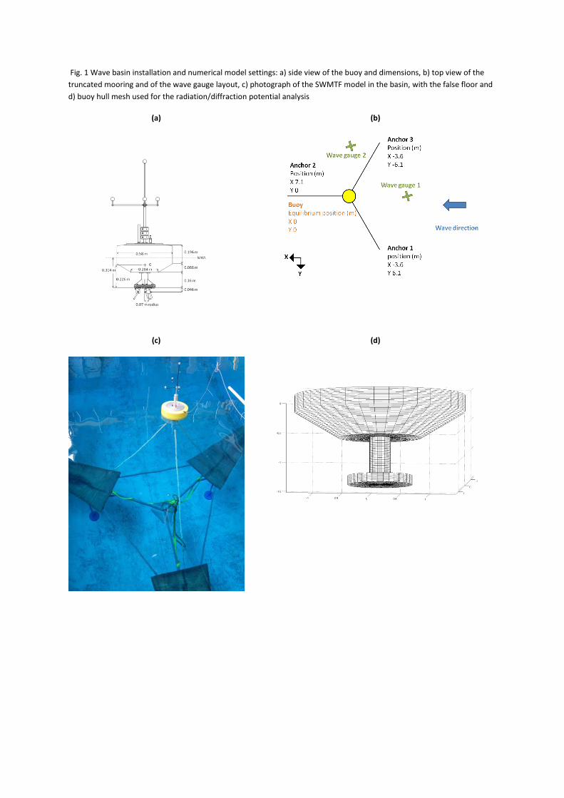
Fig. 1 Wave basin installation and numerical model settings: a) side view of the buoy and dimensions, b) top view of the
truncated mooring and of the wave gauge layout, c) photograph of the SWMTF model in the basin, with the false floor and
d) buoy hull mesh used for the radiation/diffraction potential analysis
(a) (b)
(c) (d)
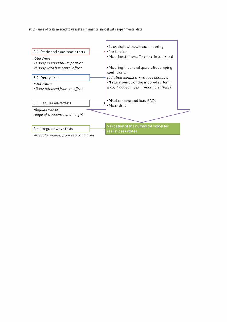
Fig. 2 Range of tests needed to validate a numerical model with experimental data
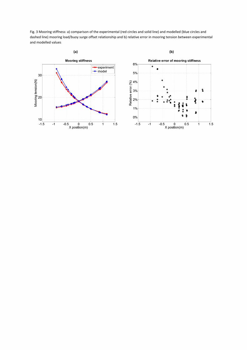
Fig. 3 Mooring stiffness: a) comparison of the experimental (red circles and solid line) and modelled (blue circles and
dashed line) mooring load/buoy surge offset relationship and b) relative error in mooring tension between experimental
and modelled values
(a) (b)

Fig. 4 Example of calculation of the natural period and linear and quadratic damping: a) detection of peaks and troughs and
calculation of the natural period, b) calculation of the linear p1 and quadratic p2 damping coefficients using a linear fit;
norm of the residua l= 0.036
(a) (b)

Fig. 5 Time-series of decay tests in a) surge, with comparison between the experimental values (red solid line), initial
(dashed black line) and corrected numerical model (blue dotted line) and in b) pitch, with a plot of the experimental surge
motion to show the coupling between surge and pitch
(a) (b)

Fig. 6 Sensitivity analysis for the surge decay: a) for the added mass; b) for the quadratic damping; c) for the linear damping
(a)
(b)
(c)

Fig. 7 Review of tests in regular waves: a) Wave heights, H, and wave periods, T, used for the tank tests. b) Selection of
steep waves, the green line is for D
KC
14.0
2
1 , separating the steep and the linear waves, and the blue line for
DKC
14.0 , separating steep waves and breaking waves. The black filled circles indicate steep waves while the red
hollow circles indicate linear waves
(a) (b)

Fig. 8 Examples of fit of the experimental surge motion: a) for H = 0.1 m and T = 1.7 s (blue line: signal, black line: fit); b)
Summary of the correlation coefficient between the fit and the experimental values c) Examples of fit for H = 0.05 m and T
= 0.9 s where a low frequency motion on the X axis can be observed (blue line: signal, black line: fit)
(a)
(b)
(c)

Fig. 9 Mean drift divided by the square of the wave amplitude for different wave frequencies and wave steepness values.

Fig. 10 Motion RAOs for the surge, heave and pitch (from top to bottom): amplitudes (left) and phases (right)
(a) (b)
(c) (d)
(e) (f)

Fig. 11 Regular wave tank test with the highest pitch RAO (H = 0.03 m and T = 1.08 s). a) Time series of the surface
elevation and pitch motion b) Picture of the buoy at its maximum pitch RAO
(a) (b)
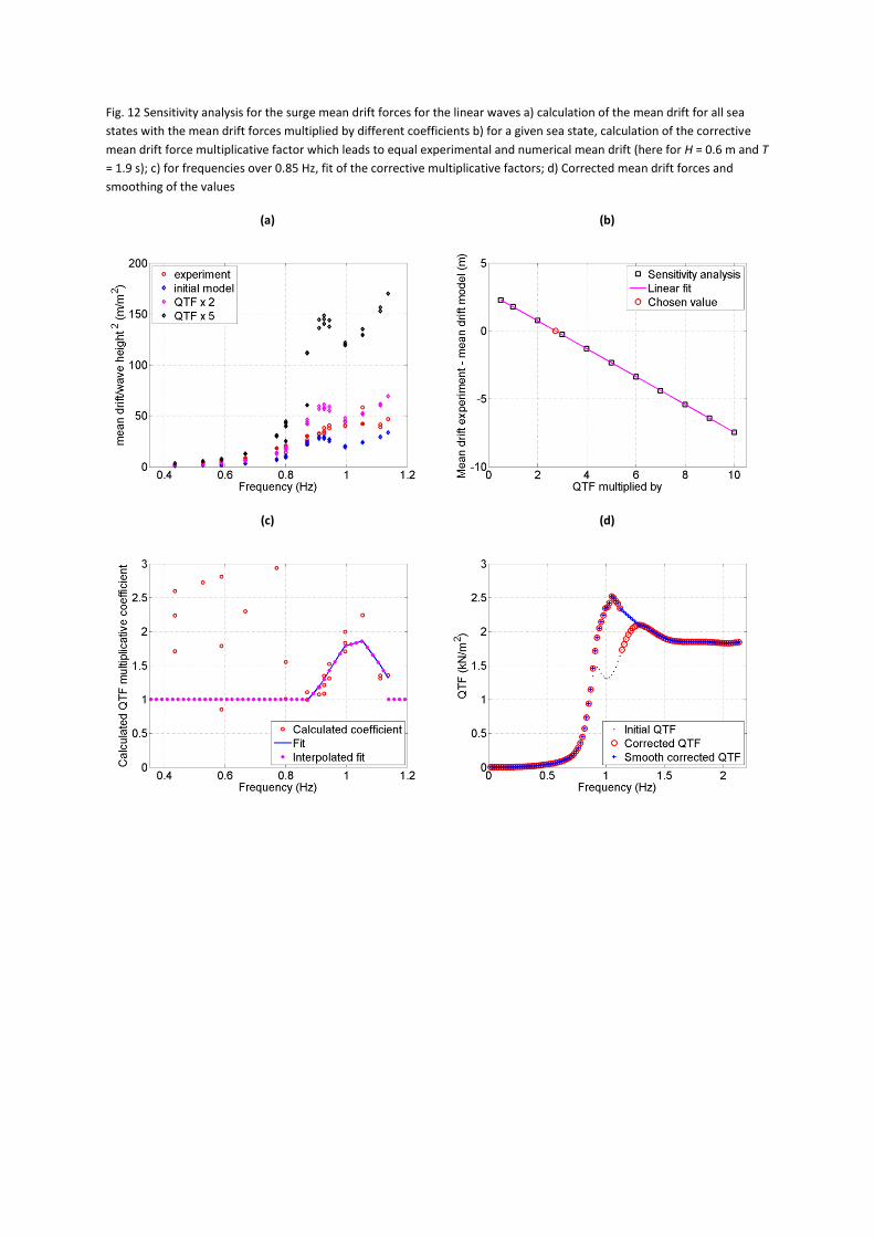
Fig. 12 Sensitivity analysis for the surge mean drift forces for the linear waves a) calculation of the mean drift for all sea
states with the mean drift forces multiplied by different coefficients b) for a given sea state, calculation of the corrective
mean drift force multiplicative factor which leads to equal experimental and numerical mean drift (here for H = 0.6 m and T
= 1.9 s); c) for frequencies over 0.85 Hz, fit of the corrective multiplicative factors; d) Corrected mean drift forces and
smoothing of the values
(a) (b)
(c) (d)
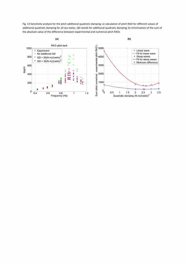
Fig. 13 Sensitivity analysis for the pitch additional quadratic damping: a) calculation of pitch RAO for different values of
additional quadratic damping for all sea states. QD stands for additional quadratic damping; b) minimisation of the sum of
the absolute value of the difference between experimental and numerical pitch RAOs
(a) (b)

Fig. 14 Example of wave inputs for Case 2. The red dots are the signal measured during the experiment and the blue dots
are for the corrected signal used as an input in the numerical model with different sampling frequencies: a) 100 Hz, b) 10
Hz, c) 4 Hz
(a)
(b)
(c)

Fig. 15 Example of motion time series for Case 2: a) surge motion, b) heave motion and c) pitch motion. Red line:
experiment, thick blue line: numerical model
(a)
(b)
(c)
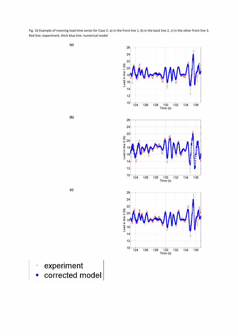
Fig. 16 Example of mooring load time series for Case 2: a) in the front line 1, b) in the back line 2, c) in the other front line 3.
Red line: experiment, thick blue line: numerical model
(a)
(b)
(c)

Fig. 17 Example of mooring load time series for Case 2 using different parameters for the numerical model: a) surge
motion, b) heave motion, c) pitch motion, d) in the front line 1, e) in the back line 2, f) in the other front line 3. Solid red
line: experiment, blue dashed line: numerical model with full QTFs, black dotted line: numerical model using Newman’s
approximation with diagonal corrections
(a) (d)
(b) (e)
(c) (f)
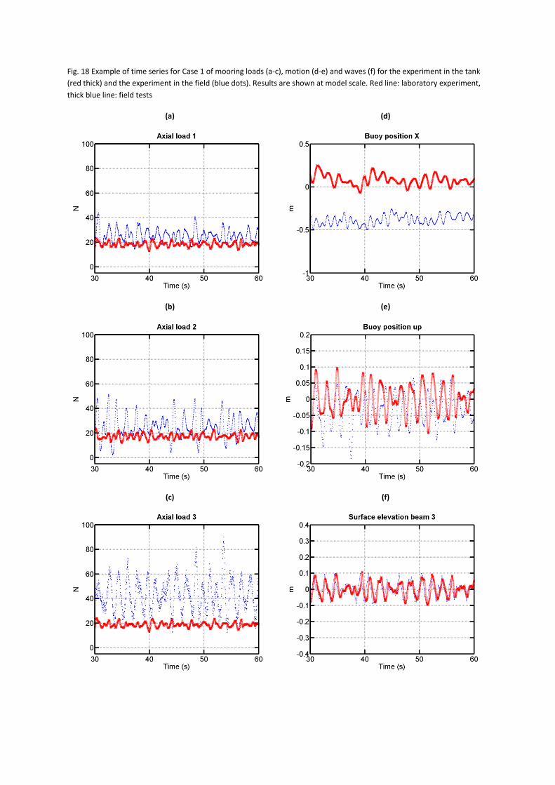
Fig. 18 Example of time series for Case 1 of mooring loads (a-c), motion (d-e) and waves (f) for the experiment in the tank
(red thick) and the experiment in the field (blue dots). Results are shown at model scale. Red line: laboratory experiment,
thick blue line: field tests
(a) (d)
(b) (e)
(c) (f)

Fig. 19 Variations in motions and loads for Case 2 with models using different rope stiffness: a) Normalised correlation
coefficient between the model with a given stiffness and the model used in this study; b) Normalised maximum mooring
load with the models using different stiffness
(a) (b)

Table 1 Properties of the original mooring lines and of the simplified, scaled and truncated mooring lines
where Cdn and Cmn are normal drag and inertia coefficients, Cda and Cma are axial drag and inertia
coefficients, T = tonnes
Section:
top(1) to
bottom (4)
Section
simplified
mooring
Components of
full scale SWMTF
mooring
Length
(m)
Nominal
diameter
(m)
Mass (kg/m) Axial stiffness
(EA, kN)
Drag
coefficient
Inertia
coefficient
In air In
water
Cdn Cda Cmn Cma
1 Chain Swinging arm 4x9.5T shackle rope thimble load cell 10T swivel 25T shackle large rope thimble
0.259 0.008 1.753 1.529 6464 1 0.4 1 0.07
2 Rope Nylon rope: Bridon
superline 44mm
diameter 4.0 0.009 0.024 0.00425
Scaled value for
full scale
facility:7.1-7.8
Tank (mean):
10.873
1.6 0 1 0
3 Chain 2x9.5T shackle
10T swivel
25T shackle
large rope thimble
0.126 0.006 1.786 1.558 3.636e6 1 0.4 1 0.07
4 Chain DN24 openlink
chain
9.5T shackle
5.672 0.0049 0.4609 0.402 2.0505e6 1 0.4 1 0.08

Table 2 Full scale and model buoy properties and difference with theoretical values where COG=centre of
gravity
Full scale SWMTF values Theoretical scaled values Measured scaled values Relative error
Mass (kg) 3108 24.86 24.86 0% Distance between COG and
bottom of keel (m)
1.13 0.2260 0.2262 0.09%
Moment of inertia Ixx (kg.m2) 4260.75 1.3634 1.4141 3.72%
Moment of inertia Izz (kg.m2) 1178.83 0.3772 0.3963 5.06%

Table 3 Results for the surge decay tests: amplitude of release and after one oscillation, natural period Tm,
linear damping p1 and quadratic damping p2, and norm of the residuals associated with the damping linear
fit
Surge Mean Standard deviation
Amplitude of
release(m) /
amplitude after 1
oscillation (m)
Exp. 1 -0.69/-0.076
Mean(abs) =
0.70/0.084
Std(abs) =
0.075/0.0078
Exp. 2 -0.59/-0.083
Exp. 3 -0.82/-0.074
Exp. 4 0.70/0.092
Exp. 5 0.67/0.090
Exp. 6 0.73/0.090
Natural period Tm
(s)
Exp. 1 11.06
11.11 0.0447
Exp. 2 11.09
Exp. 3 11.11
Exp. 4 11.14
Exp. 5 11.10
Exp. 6 11.19
p1 (s-1 ) Exp. 1 0.03133
0.0393 0.0127
Exp. 2 0.02737
Exp. 3 0.02688
Exp. 4 0.04234
Exp. 5 0.05554
Exp. 6 0.05249
p2 (m-1 ) Exp. 1 4.876
5.0949 0.3036
Exp. 2 4.643
Exp. 3 5.119
Exp. 4 5.227
Exp. 5 5.523
Exp. 6 5.181
Norm of the
residuals
Exp. 1 0.05360
0.1041 0.0750
Exp. 2 0.03701
Exp. 3 0.03732
Exp. 4 0.1121
Exp. 5 0.2150
Exp. 6 0.1697

Table 4 Results for the pitch decay tests: amplitude of release, natural period Tm, linear damping p1 and
quadratic damping p2, and norm of the residuals associated with the damping linear fit
Pitch Mean Standard
deviation
Amplitude of
release(°) /
amplitude after 1
oscillation (°)
Exp. 1 -7.3/-4.0
Mean(abs) =
3.7/2.3
Std(abs) =
2.1/1.1
Exp. 2 -3.0/-2.1
Exp. 3 -3.6/-2.4
Exp. 4 -3.2/-2.2
Exp. 5 1.6/0.93
Natural period Tm
(s)
Exp. 1 1.070
/ / Exp. 2 1.080
Exp. 3 1.095
Exp. 4 1.120
Exp. 5 1.088
p1 (s-1 ) Exp. 1 /
/ / Exp. 2 /
Exp. 3 -0.5105
Exp. 4 /
Exp. 5 0.01242
p2 (rad-1 ) Exp. 1 /
/ / Exp. 2 /
Exp. 3 0.9197
Exp. 4 /
Exp. 5 0.3268
Norm of the
residuals
Exp. 1 /
/ / Exp. 2 /
Exp. 3 0.8512
Exp. 4 /
Exp. 5 0.1585

Table 5 Comparison of experimental and numerical results: natural period Tm, linear damping p1 and
quadratic damping p2 for surge decay
Values measured from
tank
Initial numerical model:
value/relative error
Corrected numerical
model: value/relative
error
Natural Period Tm (s) 11.11 10.68/4% 11.20/1% p1 (s
-1 ) 0.0393 0.0008/98% 0.0426/ 8%
p2 (m-1 ) 5.0949 1.0503/79% 4.7488/7%

Table 6 Correction implemented on added mass, linear damping p1 and quadratic damping p2 for the surge
motion
Added mass
multiplied by
Additional Linear
damping p1 (s-1)
Additional Quadratic
Damping p2(m-1)
1.3262 0.0487 4.2639

Table 7 Statistical properties of the irregular sea states as calculated by WavesMon, the ADCP firmware
using the field data, and plot of the field data spectrum with WAFO function dat2spec [20], using default
frequency smoothing (parzen window function on the estimated autocovariance function)
Case HS (m) TP (s) HS full scale (m) TP full scale(s) Spectrum model scale based on field test data
1 0.23 1.88 1.15 4.20
2 0.10 1.30 0.50 2.91
3 0.29 2.91 1.45 6.51

Table 8 Comparison of experimental measurements and numerical model results for the wave elevation,
buoy motions and mooring loads
Wave Motion Load in mooring line
Correlation coefficients between the experiments and the numerical model Case Elevation X Z pitch Line 1 Line 2 Line 3
1 0.99 0.79 0.96 0.91 0.76 0.84 0.77
2 0.99 0.93 0.96 0.92 0.83 0.85 0.80
3 0.99 0.77 0.96 0.82 0.75 0.79 0.75
Standard deviations: experiment/numerical model/relative error
Case Elevation (m) X (m) Z (m) Pitch (deg(deg) Line 1 (N) Line 2 (N) Line 3 (N)
1 0.054/0.053/1% 0.118/0.070/41% 0.052/0.053/2% 6.2/7.2/15% 2.7/2.0/28% 2.8/2.1/26% 2.8/2.0/29%
2 0.028/0.028/1% 0.073/0.053/27% 0.028/0.027/3% 5.1/5.4/5% 1.7/1.3/26% 2.2/1.6/27% 1.7/1.3/25%
3 0.077/0.078/1% 0.136/0.098/28% 0.077/0.078/1% 6.8/7.7/13% 3.3/2.4/28% 3.2/2.4/23% 3.4/2.4/30%

Table 9 Comparison of maximum mooring loads for the different cases and the different mooring lines
Case Line 1 (N) Line 2 (N) Line 3 (N)
1 Experiment 33.9 31.2 34.9 Corrected Model. 28.9 25.2 28.9
Relative error 15% 8% 12%
2 Experiment 27.4 25.0 27.7
Corrected Model. 25.9 23.7 28.2
Relative error 17% 5% 6%
3 Experiment 32.9 29.8 33.7
Corrected Model. 28.9 25.2 28.9
Relative error 17% 9% 14%

Table 10 Comparison of correlation coefficients between the numerical model results using different
sampling frequencies for the wave input and the experimental results for the wave elevation, buoy motions
and mooring loads for Case 1
Wave Motion Load in mooring line
Correlation coefficients between the experiments and the numerical model/relative error with 100 Hz input Freq
wave
input
Elevation X Z pitch Line 1 Line 2 Line 3
4 Hz 0.9927/0.40% 0.8041/2.15% 0.9629/0.01% 0.9089/0.12% 0.7611/0.17% 0.8396/0.25% 0.7728/0.03%
10
Hz
0.9962/0.05% 0.8122/1.17% 0.9626/0.02% 0.9075/0.03% 0.7589/0.12% 0.8408/0.11% 0.7719/0.09%
100
Hz
0.9967/0% 0.8218/0% 0.9628/0% 0.9078/0% 0.7598/0% 0.8417/0% 0.7726/0%

Table 11 Comparison of correlation coefficients between the numerical model results using the Newman’s
approximation (before and after correction of the mean drift) and using the full QTFs for the buoy motions
and mooring loads for Case 1
Motion Load in mooring line
Correlation coefficients between the experiment and the numerical models Method of calculation X Z pitch Line 1 Line 2 Line 3
Newman’s approximation original 0.8087 0.9628 0.9094 0.7593 0.8414 0.7702
Newman’s approximation corrected 0.8041 0.9629 0.9089 0.7611 0.8396 0.7728
Full QTFs 0.7281 0.9627 0.7569 0.7206 0.8040 0.7239
Full QTFs diagonal corrected 0.7189 0.9627 0.7320 0.7104 0.8046 0.7189
Mean values/relative error with experiment
Method of calculation X (m) Line 1 (N) Line 2 (N) Line 3 (N)
Newman’s approximation original 0.099/23% 18.7/1% 17.4/2% 18.7/2%
Newman’s approximation corrected 0.118/9% 18.8/1% 17.2/1% 18.8/1%
Full QTFs 0.099/23% 18.9/2% 17.6/3% 18.9/0%
Full QTFs diagonal corrected 0.119/8% 19.0/3% 17.5/2% 19.1/1%
Experiment 0.129 18.5 17.1 19.0
Max values/relative error with experiment
Method of calculation Line 1 (N) Line 2 (N) Line 3 (N)
Newman’s approximation original 28.9/15% 26.3/16% 28.9/17%
Newman’s approximation corrected 28.9/15% 25.9/17% 28.9/17%
Full QTFs 32.8/3% 29.7/5% 29.5/16%
Full QTFs diagonal corrected 33.0/3% 27.4/12% 29.5/15%
Experiment 33.9 31.2 34.9
Std values/relative error with experiment
Method of calculation X (m) Z (m) Pitch (°) Line 1 (N) Line 2 (N) Line 3 (N)
Newman’s approximation original 0.065/45% 0.053/2% 7.2/16% 2.0/28% 2.1/25% 2.0/30%
Newman’s approximation corrected 0.070/41% 0.053/2% 7.2/16% 2.0/28% 2.1/26% 2.0/29%
Full QTFs 0.066/44% 0.053/2% 5.6/10% 2.1/23% 2.2/20% 2.1/23%
Full QTFs diagonal corrected 0.066/44% 0.053/2% 5.5/11% 2.1/23% 2.2/21% 2.1/23%
Experiment 0.118 0.052 6.2 2.7 2.8 2.8

Table 12 Comparison of mean and standard deviations between the tank test results and the field test
results for the wave elevation, buoy motions and mooring loads. Results are given at the model scale.
Wave Motion Load in mooring line
Mean field/tank/relative error Case X (m) Line 1 (N) Line 2 (N) Line 3 (N)
1 -0.388/0.129/133%
26.6/18.5/30% 25.2/17.1/32% 44.3/19.0/57%
2 -0.314/0.075/124% 23.9/18.3/23% 27.6/17.4/37% 32.9/18.6/43%
3 -0.155/0.169/209% 17.6/18.3/4% 28.1/15.5/45% 60.9/18.2/70%
Standard deviation field/tank/relative error Case Elevation (m) X (m) Z (m) Line 1 (N) Line 2 (N) Line 3 (N)
1 0.059/0.054/10%
0.059/0.118/100% 0.054/0.052/4% 6.2/2.7/56% 10.4/2.8/73% 15.8/2.8/82%
2 0.030/0.028/8% 0.046/0.073/57% 0.030/0.028/5% 2.9/1.7/41% 5.9/2.2/63% 8.2/1.7/79%
3 0.085/0.077/9% 0.062/0.136/120% 0.062/0.077/24% 5.3/3.3/37% 10.5/3.2/70% 16.5/3.4/79%


![Numerical model validation for mooring systems: Method …standards [14] for the nylon lines and from the Orcaflex™ manual [15] for the chains. The axial stiffness of three samples](https://img.pdfslide.net/doc/110x75/60cde808aef8864b8578ec96/numerical-model-validation-for-mooring-systems-method-standards-14-for-the-nylon.jpg)


![Numerical model validation for mooring systems: Method and ...123 (PTO) system [4]. Consequently, the mooring system is commonly represented in a simplified form which does not 124](https://img.pdfslide.net/doc/110x75/5e6dda2a309954236967b62a/numerical-model-validation-for-mooring-systems-method-and-123-pto-system.jpg)