NUMERICAL MODELING OF AIR DISTRIBUTION IN A TEST ROOM …

49

Simulation of Physical Processes

DOI: 10.18721/JPM.13305УДК 532.517

NUMERICAL MODELING OF AIR DISTRIBUTION IN A TEST ROOM WITH 2D SIDEWALL JET.

I. Foundations for eddy-resolving approach application based on periodical formulation

M.A. Zasimova1, N.G. Ivanov1, D. Markov2

1 Peter the Great St. Petersburg Polytechnic University, St. Petersburg, Russian Federation;2 Technical University of Sofia, Sofia, Bulgaria

The paper presents the methods and results of numerical modeling of turbulent airflow in a test room based on the vortex-resolving wall-modeled large eddy simulation approach. The room ventilation is provided by a plain air jet at Re = 5233. The jet is supplied from a slit placed at a side wall under the ceiling. The room geometry and airflow parameters correspond to the experimental benchmark test by Nielsen et al. (1978), but with the periodicity boundary conditions in the transverse direction. Calculations were carried out with the ANSYS Fluent software using fine grids consisting of up to 6x107 cells. The paper presents detailed analysis of parametric computations aimed at the evaluation of numerical simulation adequacy. In particular, the grid dependency study was performed and the Kolmogorov scale was estimated.

Keywords: turbulent airflow, plain jet, Large Eddy Simulation, ventilation

Citation: Zasimova M.A., Ivanov N.G., Markov D., Numerical modeling of air distribution in a test room with 2D sidewall jet. I. Foundations for eddy resolving approach application based on periodical formulation, St. Petersburg Polytechnical State University Journal. Physics and Mathematics. 13 (3) (2020) 49–64. DOI: 10.18721/JPM.13305

This is an open access article under the CC BY-NC 4.0 license (https://creativecommons.org/licenses/by-nc/4.0/)

ЧИСЛЕННОЕ МОДЕЛИРОВАНИЕ ЦИРКУЛЯЦИИ ВОЗДУХА В ПОМЕЩЕНИИ ПРИ ПОДАЧЕ ИЗ ПЛОСКОЙ ЩЕЛИ.

I. Отработка применения вихреразрешающего подхода с использованием периодической постановки

М.А. Засимова1, Н.Г. Иванов1, Д. Марков2

1 Санкт-Петербургский политехнический университет Петра Великого,Санкт-Петербург, Российская Федерация;

2 Софийский технический университет, София, Болгария

Представлены методика и результаты численного моделирования турбулентного течения воздуха в тестовом помещении на основе вихреразрешающего подхода – метода моделирования крупных вихрей с пристенным моделированием. Вентиляция помещения осуществляется плоской воздушной струей, подаваемой из расположенного под потолком на торцевой стенке щелевого отверстия, при значении числа Рейнольдса Re = 5233. Геометрия помещения и параметры течения соответствуют классическому тестовому эксперименту (Nielsen et al., 1978), однако задача ставилась как периодическая, что справедливо для помещения, сильно вытянутого в поперечном направлении. Расчеты в программном пакете ANSYS Fluent выполнены с использованием весьма подробных сеток размерностью до 6·107 ячеек. Подробно описаны результаты методических расчетов, направленных на оценку адекватности выполненного численного моделирования, в частности проведен анализ сеточной зависимости и дана оценка колмогоровского масштаба для рассматриваемого течения.

St. Petersburg State Polytechnical University Journal. Physics and Mathematics 13 (3) 2020

50

Ключевые слова: турбулентное течение, плоская струя, метод моделирования крупных вихрей, вентиляция

Ссылка при цитировании: Засимова М.А., Иванов Н.Г., Марков Д. Численное моделирование циркуляции воздуха в помещении при подаче из плоской щели. I. Отработка применения вихреразрешающего подхода с использованием периодической постановки // Научно-технические ведомости СПбГПУ. Физико-математические науки. 2020. Т. 13. 3. С. 56–74. DOI: 10.18721/JPM.13305

Статья открытого доступа, распространяемая по лицензии CC BY-NC 4.0 (https://creativecommons.org/licenses/by-nc/4.0/)

IntroductionOne of the challenges posed in design and

modernization of buildings is configuring the heating, ventilation and air conditioning (HVAC) systems controlling the microclimate. Comfort and safety are ensured in the living quarters by maintaining the parameters of the air (air velocity, temperature, concentration of harmful impurities, etc.) within the required range, which largely depends on the air supply scheme for the ventilation system. In this regard, improving the accuracy of assessing the quality of the air provided by the ventilation system is an issue that is steadily gaining importance.

Methods of computational fluid dynamics allowing to carry out three-dimensional simulation of turbulent jet flows have been increasingly popular in the recent years. Approaches that estimate the flow parameters based on numerically solving the steady/unsteady Reynolds-averaged Navier–Stokes equations (RANS/URANS) have become widely popular in engineering practice. The RANS/URANS approaches were employed, for example, for designing and/or modernizing the ventilation systems for a swimming pool [1], an ice rink [2], a university assembly hall of historical and architectural value [3], the interior of St. Isaac’s Cathedral in St. Petersburg [4].

Methods of computational fluid dynamics turn out to be even more important for developing life support systems than ventilation systems for buildings, since almost every proposed solution is unique. An example of solving such problems are the computations of ventilation for crew and passenger cabins of aircraft [5, 6]. Over the past two decades, the RANS/URANS approaches have been used to assess the performance and efficiency of life support systems for spacecraft. In particular, calculations of the atmosphere at the International Space Station (ISS) were carried out under standard conditions [7], as well as after using a carbon dioxide fire extinguisher in the US Orbital Segment of the ISS [8].

Despite examples of successful solutions to applied ventilation problems, the accuracy of the calculation results for air distribution in rooms obtained by the RANS/URANS approaches remains an open question. The degree of uncertainty in the results of RANS/URANS calculations can be estimated either by direct comparison of the calculated results with the data of a physical experiment, or by comparing the RANS/URANS results with the data obtained by more accurate eddy-resolving approaches to describing turbulent flows.

Direct Numerical Simulation (DNS) from first principles can be used as an eddy-resolving approach. Full Navier–Stokes equations are solved within the DNS approach, which allows to describe all scales of turbulence if applied correctly. It is well known that the DNS approach requires huge computational costs and its application is limited to very moderate values of the Reynolds number. An alternative for numerical studies with manageable computational costs is the Large Eddy Simulation method (LES). The LES approach involves solving filtered Navier–Stokes equations, allowing to describe the behavior of large eddies in combination with semi-empirical simulation of small-scale eddies. The LES method not only makes it possible to carry out fundamental studies, including those aimed at assessing the accuracy of RANS simulation, but is also gaining ground for solving applied problems [9], including in modeling ventilation flows characterized by relatively moderate Reynolds numbers, and also, in most cases, fairly mild requirements for near-wall resolution.

Different studies modeled HVAC systems using the LES approach. Simulation of air exchange by the LES approach was first presented in [10], considering the ventilation in a test room of a simple shape, with experimental data available [11]. A more complex problem of flow in a relatively cluttered room equipped with a displacement ventilation system is solved in [12]. Ref. [13]

51


presents air distribution estimates carried out by LES for the Columbus orbital module, which is part of the ISS, equipped with a multi-jet ventilation system; the calculation results were also compared with experimental data. Later, the LES approach was used to determine the parameters of air exchange in a university lecture hall [14] and in the premises of a residential building [15].

The practical application of the LES approach needs to further refined by solving test problems. This study describes and tests the procedure for applying the Wall-Modeled LES approach (WMLES). The well-known test problem of ventilation flow in a room where a plain air jet is supplied from a slit located under the ceiling [11] was chosen as the object of research. Detailed experimental data are available for this test on the distributions of the velocity components and their fluctuations, measured using Laser Doppler Anemometry (LDA). The test room in [11] was a rectangular parallelepiped with a square cross section; however, in this study, we formulated a three-dimensional problem with periodic conditions imposed in the transverse direction, which is to say that the side walls were excluded from consideration.

This statement makes it possible to correctly reproduce the flow structure only in the central part of the room, without affecting the three-dimensional structure of secondary

flows. The clear advantage of such a “quasi-two-dimensional” simplified statement was that it made it possible to carry out a series of parametric calculations, considerably optimizing the computational costs.

We present the results of systematic calculations, and recommendations for applying the WMLES method developed based on these results.

The sidewall effect is considered in the second part of this study, published as a separate paper [16], providing a detailed comparison of the calculation results in a complete statement, without assuming periodic flow [11].

Problem statement

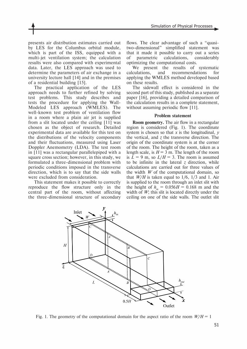
Room geometry. The air flow in a rectangular region is considered (Fig. 1). The coordinate system is chosen so that x is the longitudinal, y the vertical, and z the transverse direction. The origin of the coordinate system is at the corner of the room. The height of the room, taken as a length scale, is H = 3 m. The length of the room is L = 9 m, so L/H = 3. The room is assumed to be infinite in the lateral z direction, while calculations are carried out for three values of the width W of the computational domain, so that W/H is taken equal to 1/6, 1/3 and 1. Air is supplied to the room through an inlet slit with the height of hin = 0.056H = 0.168 m and the width of W; this slit is located directly under the ceiling on one of the side walls. The outlet slit

Fig. 1. The geometry of the computational domain for the aspect ratio of the room W/H = 1


52

located near the floor on the opposite wall has a height of hout= 0.16H = 0.48 m and a width of W. A channel with a length of 0.5H adjacent to the slit is included in the computational domain to prevent the formation of return currents at the outlet boundary of the domain.

Physical parameters of the environment and boundary conditions. Isothermal motion of air described by the model of incompressible fluid with constant physical properties is considered: the density ρ = 1.23 kg/m3, the dynamic vis-cosity µ = 1.79·10–5 Pa·s.

Air is supplied to the entrance to the room at a mean flow velocity equal to Vin = 0.455 m/s. The Reynolds number computed from the height of the inlet slit is Re = ρhinVin/µ = 5233. An aux-iliary problem of air flow in a flat channel with a height of hin, also based on the WMLES method was solved before imposing the boundary con-ditions at the inlet. The transverse dimensions of the computational domain in this case corre-spond to the selected value of W/H. The velocity distributions in the section x/hin = 18 from the entrance to the channel served as the velocity profiles at the entrance to the room (a uniform profile was given at the entrance to the chan-nel), extracted from the time-averaged solution. Additional calculations were carried out for the case with the transverse size W/H= 1/6, giving a uniform velocity profile, as well as the inlet pro-file extracted from the solution to the problem of flow in the channel in the section x/hin = 60 at the entrance to the room.

Periodic boundary conditions were imposed at the lateral boundaries along the z direction. Soft boundary conditions were imposed at the outlet boundary. The remaining boundaries of the computational domain were solid walls on which the no-slip conditions were imposed.

Turbulence simulation. Turbulent air flow was simulated using the eddy-resolving WMLES approach, which is based on solving the filtered Navier–Stokes equations (see, for example, [9]). The instantaneous variables f are replaced by the sum of the filtered and subgrid-scale variables:

F = f + f ′. The value of f is determined by the expression

f x t G x x f x t dxVol

( , ) ( , ) ( , ) ,= − ′ ′ ′∫ ∆ 3(1)

where G(x – x′, Δ) is the filter function determining the size and structure of small-scale turbulence (for example, a box filter); x is the coordinate of the point under consideration, ∆ is the characteristic filter size (filter width).

Eddies whose size is smaller than the filter width are not resolved.

The filtered Navier–Stokes equations for incompressible fluid with constant physical properties can be written in the following form:

VV VV

0

12

;

( )

( ) ,

t

p S

SGS(2)

where V is the velocity vector with the com-ponents (Vx, Vy, Vz); S is the strain rate tensor; τSGS is the term resulting from spatial filtering of the equations.

The generalized Boussinesq hypothesis is used to determine the subgrid-scale stresses:

ijSGS

kk ij SGS ijS 1

32 , (3)

where νSGS, m2/s, is the subgrid-scale turbu-

lent viscosity to be found using some subgrid model.

The classical subgrid-scale model is the algebraic Smagorinsky model, proposed back in 1963 [17]. Based on dimensional analysis, the subgrid-scale viscosity in this model is expressed in terms of filter size and the magnitude of the strain-rate tensor:

νSGS = (CSΔ)2S,where CS = 0.2 is the empirical Smagorinsky constant.

The computational grid acts as the filter in practical implementations of the LES approach, with Δ usually defined as the cube root of the volume of the grid cell.

The WMLES S-Omega approach was used in our calculations; its practical implementation is based on the data given in [18]. Compared with the classical Smagorinsky model, the subgrid-scale viscosity is determined here using a modified linear subgrid scale, a damping factor (similar to the Van Driest factor in the Prandtl model for the RANS approach), and the difference |S – Ω| instead of the magnitude of the strain-rate tensor S:

SGS w Sd C

S y

min ,

exp / ,

2 2

3

1 25

(4)

53


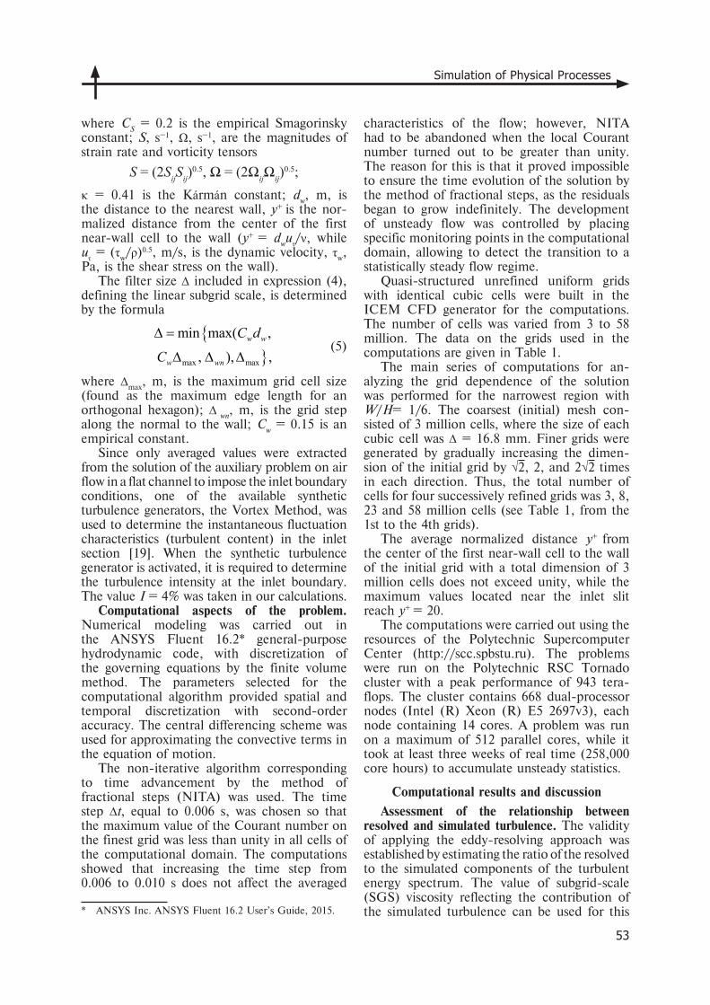
where CS = 0.2 is the empirical Smagorinsky constant; S, s–1, Ω, s–1, are the magnitudes of strain rate and vorticity tensors

S = (2SijSij)0.5, Ω = (2ΩijΩij)

0.5;κ = 0.41 is the Kármán constant; dw, m, is the distance to the nearest wall, y+ is the nor-malized distance from the center of the first near-wall cell to the wall (y+ = dwuτ/ν, while uτ = (τw/ρ)0.5, m/s, is the dynamic velocity, τw, Pa, is the shear stress on the wall).

The filter size ∆ included in expression (4), defining the linear subgrid scale, is determined by the formula

min max( ,

, ), ,max max

C d

Cw w

w wn

(5)

where ∆max, m, is the maximum grid cell size (found as the maximum edge length for an orthogonal hexagon); ∆ wn, m, is the grid step along the normal to the wall; Cw = 0.15 is an empirical constant.

Since only averaged values were extracted from the solution of the auxiliary problem on air flow in a flat channel to impose the inlet boundary conditions, one of the available synthetic turbulence generators, the Vortex Method, was used to determine the instantaneous fluctuation characteristics (turbulent content) in the inlet section [19]. When the synthetic turbulence generator is activated, it is required to determine the turbulence intensity at the inlet boundary. The value I = 4% was taken in our calculations.

Computational aspects of the problem. Numerical modeling was carried out in the ANSYS Fluent 16.2* general-purpose hydrodynamic code, with discretization of the governing equations by the finite volume method. The parameters selected for the computational algorithm provided spatial and temporal discretization with second-order accuracy. The central differencing scheme was used for approximating the convective terms in the equation of motion.

The non-iterative algorithm corresponding to time advancement by the method of fractional steps (NITA) was used. The time step ∆t, equal to 0.006 s, was chosen so that the maximum value of the Courant number on the finest grid was less than unity in all cells of the computational domain. The computations showed that increasing the time step from 0.006 to 0.010 s does not affect the averaged

* ANSYS Inc. ANSYS Fluent 16.2 User’s Guide, 2015.

characteristics of the flow; however, NITA had to be abandoned when the local Courant number turned out to be greater than unity. The reason for this is that it proved impossible to ensure the time evolution of the solution by the method of fractional steps, as the residuals began to grow indefinitely. The development of unsteady flow was controlled by placing specific monitoring points in the computational domain, allowing to detect the transition to a statistically steady flow regime.

Quasi-structured unrefined uniform grids with identical cubic cells were built in the ICEM CFD generator for the computations. The number of cells was varied from 3 to 58 million. The data on the grids used in the computations are given in Table 1.

The main series of computations for an-alyzing the grid dependence of the solution was performed for the narrowest region with W/H= 1/6. The coarsest (initial) mesh con-sisted of 3 million cells, where the size of each cubic cell was ∆ = 16.8 mm. Finer grids were generated by gradually increasing the dimen-sion of the initial grid by √2, 2, and 2√2 times in each direction. Thus, the total number of cells for four successively refined grids was 3, 8, 23 and 58 million cells (see Table 1, from the 1st to the 4th grids).

The average normalized distance y+ from the center of the first near-wall cell to the wall of the initial grid with a total dimension of 3 million cells does not exceed unity, while the maximum values located near the inlet slit reach y+ = 20.

The computations were carried out using the resources of the Polytechnic Supercomputer Center (http://scc.spbstu.ru). The problems were run on the Polytechnic RSC Tornado cluster with a peak performance of 943 tera-flops. The cluster contains 668 dual-processor nodes (Intel (R) Xeon (R) E5 2697v3), each node containing 14 cores. A problem was run on a maximum of 512 parallel cores, while it took at least three weeks of real time (258,000 core hours) to accumulate unsteady statistics.

Computational results and discussion

Assessment of the relationship between resolved and simulated turbulence. The validity of applying the eddy-resolving approach was established by estimating the ratio of the resolved to the simulated components of the turbulent energy spectrum. The value of subgrid-scale (SGS) viscosity reflecting the contribution of the simulated turbulence can be used for this


54

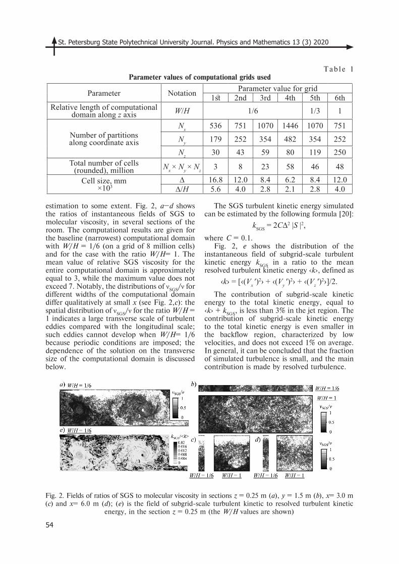
estimation to some extent. Fig. 2, a–d shows the ratios of instantaneous fields of SGS to molecular viscosity, in several sections of the room. The computational results are given for the baseline (narrowest) computational domain with W/H = 1/6 (on a grid of 8 million cells) and for the case with the ratio W/H= 1. The mean value of relative SGS viscosity for the entire computational domain is approximately equal to 3, while the maximum value does not exceed 7. Notably, the distributions of νSGS/ν for different widths of the computational domain differ qualitatively at small x (see Fig. 2,c): the spatial distribution of νSGS/ν for the ratio W/H = 1 indicates a large transverse scale of turbulent eddies compared with the longitudinal scale; such eddies cannot develop when W/H= 1/6 because periodic conditions are imposed; the dependence of the solution on the transverse size of the computational domain is discussed below.

The SGS turbulent kinetic energy simulated can be estimated by the following formula [20]:

kSGS = 2C∆2 |S |2,where C = 0.1.

Fig. 2, e shows the distribution of the instantaneous field of subgrid-scale turbulent kinetic energy kSGS in a ratio to the mean resolved turbulent kinetic energy ‹k›, defined as

‹k› = [‹(Vx ′)2› + ‹(Vy ′)

2› + ‹(Vz ′)2›]/2.

The contribution of subgrid-scale kinetic energy to the total kinetic energy, equal to ‹k› + kSGS, is less than 3% in the jet region. The contribution of subgrid-scale kinetic energy to the total kinetic energy is even smaller in the backflow region, characterized by low velocities, and does not exceed 1% on average. In general, it can be concluded that the fraction of simulated turbulence is small, and the main contribution is made by resolved turbulence.

Fig. 2. Fields of ratios of SGS to molecular viscosity in sections z = 0.25 m (a), y = 1.5 m (b), x= 3.0 m (c) and x= 6.0 m (d); (e) is the field of subgrid-scale turbulent kinetic to resolved turbulent kinetic

energy, in the section z = 0.25 m (the W/H values are shown)

Tab l e 1Parameter values of computational grids used

Parameter Notation Parameter value for grid1st 2nd 3rd 4th 5th 6th

Relative length of computational domain along z axis W/H 1/6 1/3 1

Number of partitions along coordinate axis

Nx 536 751 1070 1446 1070 751

Ny 179 252 354 482 354 252Nz 30 43 59 80 119 250

Total number of cells (rounded), million Nx × Ny × Nz 3 8 23 58 46 48

Cell size, mm ×103

∆ 16.8 12.0 8.4 6.2 8.4 12.0∆/H 5.6 4.0 2.8 2.1 2.8 4.0

55


Estimation of the Kolmogorov scale. The Kolmogorov scale η (m) is an important characteristic in simulation of turbulent flows, reflecting the characteristic size of the minimum eddies where kinetic energy dissipates due to the action of viscous friction forces. This scale determines the minimum requirements to the spatial resolution in direct numerical simulation, which must fully resolve the entire turbulent energy spectrum. The magnitude of the Kolmogorov scale is found by the formula

1/43

, ν

η = ε (6)

where ε, m2/s3, is the dissipation rate of turbulent kinetic energy per unit mass; ν, m2/s, is the kinematic viscosity.

The local values of the Kolmogorov scale for a near-ceiling jet take their minimum values in the region of the near-wall boundary layer in the initial zone of jet propagation. However, the degree of eddy resolution in the region of the near-wall boundary layer is not explicitly considered within our study; below we confine ourselves to discussing the quality of predicting wall friction by comparing solutions obtained on different grids. Quantitative estimates of the Kolmogorov scale were primarily carried out for the mixing layer whose degree of resolution is extremely important for adequately predicting the structure of the ventilation flow. Estimates of η are carried out using the computed data for the baseline (narrowest) computational domain with W/H= 1/6, while two different methods are used to determine the local dissipation rate of turbulent kinetic energy.

Method I for estimating ε. This method for determining ε to subsequently estimate the magnitude of the Kolmogorov scale η relies on the data from an additional steady RANS computation. A quasi-structured grid with the dimension of 141,000 cells clustered in the re-gion of the mixing layer and to the walls of the room, so that the value of y+ was less than unity (a grid-independent solution is taken for this grid). A uniform velocity distribution (Vin = 0.455 m/s) was set at the inlet boundary. A semiempirical RNG k-ε turbulence model was used to close the RANS equations, allow-ing to directly extract the field ε from the ob-tained numerical solution.

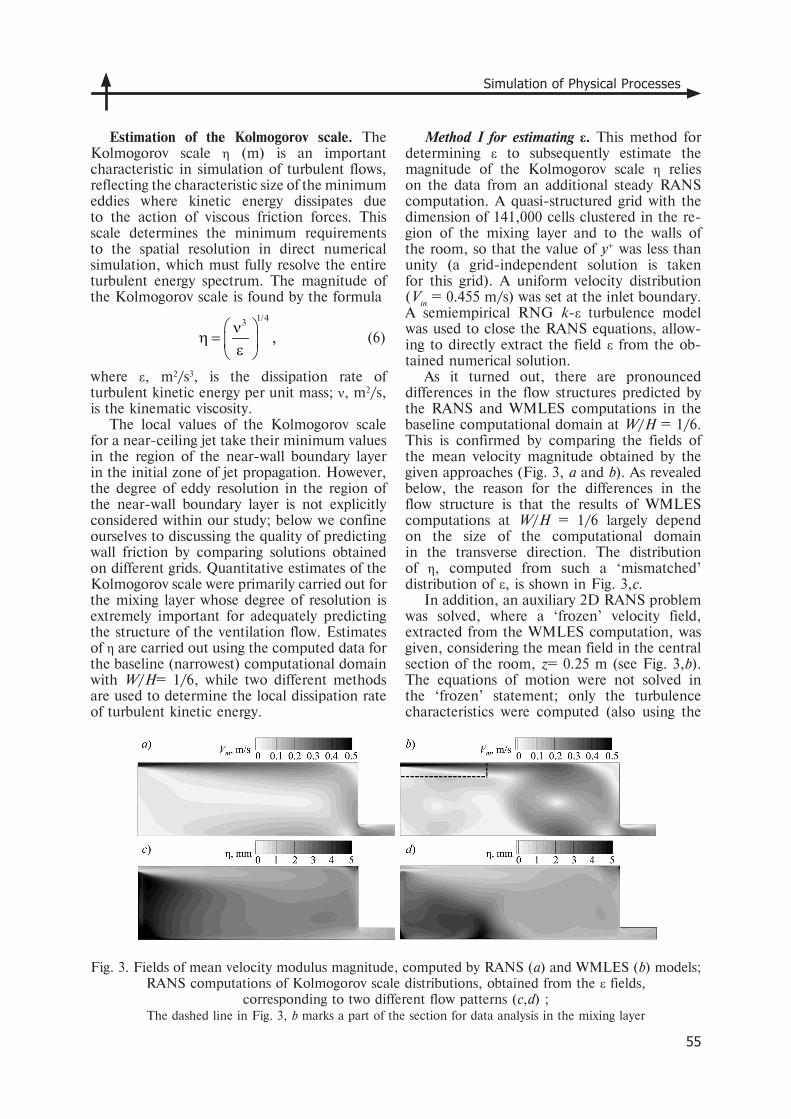
As it turned out, there are pronounced differences in the flow structures predicted by the RANS and WMLES computations in the baseline computational domain at W/H = 1/6. This is confirmed by comparing the fields of the mean velocity magnitude obtained by the given approaches (Fig. 3, a and b). As revealed below, the reason for the differences in the flow structure is that the results of WMLES computations at W/H = 1/6 largely depend on the size of the computational domain in the transverse direction. The distribution of η, computed from such a ‘mismatched’ distribution of ε, is shown in Fig. 3,c.

In addition, an auxiliary 2D RANS problem was solved, where a ‘frozen’ velocity field, extracted from the WMLES computation, was given, considering the mean field in the central section of the room, z= 0.25 m (see Fig. 3,b). The equations of motion were not solved in the ‘frozen’ statement; only the turbulence characteristics were computed (also using the

Fig. 3. Fields of mean velocity modulus magnitude, computed by RANS (a) and WMLES (b) models; RANS computations of Kolmogorov scale distributions, obtained from the ε fields,

corresponding to two different flow patterns (c,d) ; The dashed line in Fig. 3, b marks a part of the section for data analysis in the mixing layer


56

RNG k-ε model). The field of ε obtained by this method was also used to calculate the field of η (see Fig. 3,d).

It can be seen from Fig. 3, c that the lo-cal value of the Kolmogorov scale in the dis-tribution of η, computed from the field of ε corresponding to the combined RANS com-putations of the distributions of velocity and turbulent characteristics, varies from ηmin= 0.42 mm in the region of the jet mixing layer up to ηmax= 13.3 mm in the region of low-velocity flow (see Fig. 3,c, bottom left corner). The dis-tribution of the Kolmogorov scale constructed from the field of ε corresponding to the ‘frozen’ WMLES velocity field is shown in Fig. 3,d. In this case, the distribution of local values of η differed considerably from the picture shown in Fig. 3,c but the minimum value practically did not change: ηmin= 0.43 mm; the localization of the region of small values of η did not change either, while the maximum value of η in this case was ηmax= 34 mm.

Thus, the dimension of the grid for direct numerical simulation of the flow in the region W/H= 1/6 on a uniform grid of cubic elements with a linear size ηmin should be at least 182 bil-lion cells. A grid with the total dimension of at least 1100 billion cells will be required for DNS computations in the region W/H= 1, described in the experimental study [11]; in this case, the time step value should not exceed 10–3 s to en-sure the Courant number values less than unity. Importantly, these estimates do not take into account the decrease in η in the boundary layer of the near-wall jet, so grids of even higher dimensions are required to perform DNS com-putations in reality.

The results of the estimates are summarized in Table 2, listing the ratios of the linear size of the cell in the computational grid to the local minimum and maximum values of the Kolmogorov scale for the four cases considered.

Method II for estimating ε. This method for determining ε directly uses the data obtained by the LES approach based on interpreting the equation for kinetic turbulent energy:

( )

' '

' '

' '2' '

2

1

,

j jj j

jk kj

k k kj k

j j j j

k kV V kt x x

V px

V V Vk V Vx x x x

∂ ∂ ∂+ + =

∂ ∂ ∂

∂= − +

∂

∂ ∂ ∂∂+ − −

∂ ∂ ∂ ∂

δρ

ν ν

(7)

where the last term is exactly the expression for its dissipation rate,

' '

.k k

j j

V Vx x

∂ ∂ε = ν

∂ ∂(8)

The DNS approach allows to fully resolve the turbulent energy spectrum; therefore, if the dissipation rate is calculated directly by Eq. (8), it is determined exactly. The dissipation rate has a maximum in the high-frequency part of the energy spectrum, and the high-frequency part of the spectrum is simulated by the SGS viscosity in the LES method, so the value of the resolved dissipation rate calculated by Eq. (8) is underestimated compared to the exact value of ε. The value of ε increases in LES computa-tions of successively refined grids that provide a better resolution of the high-frequency region of the spectrum Accordingly, the values of η decrease, approaching the exact value.

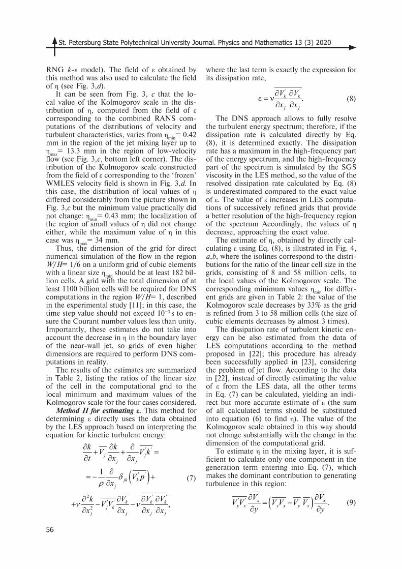
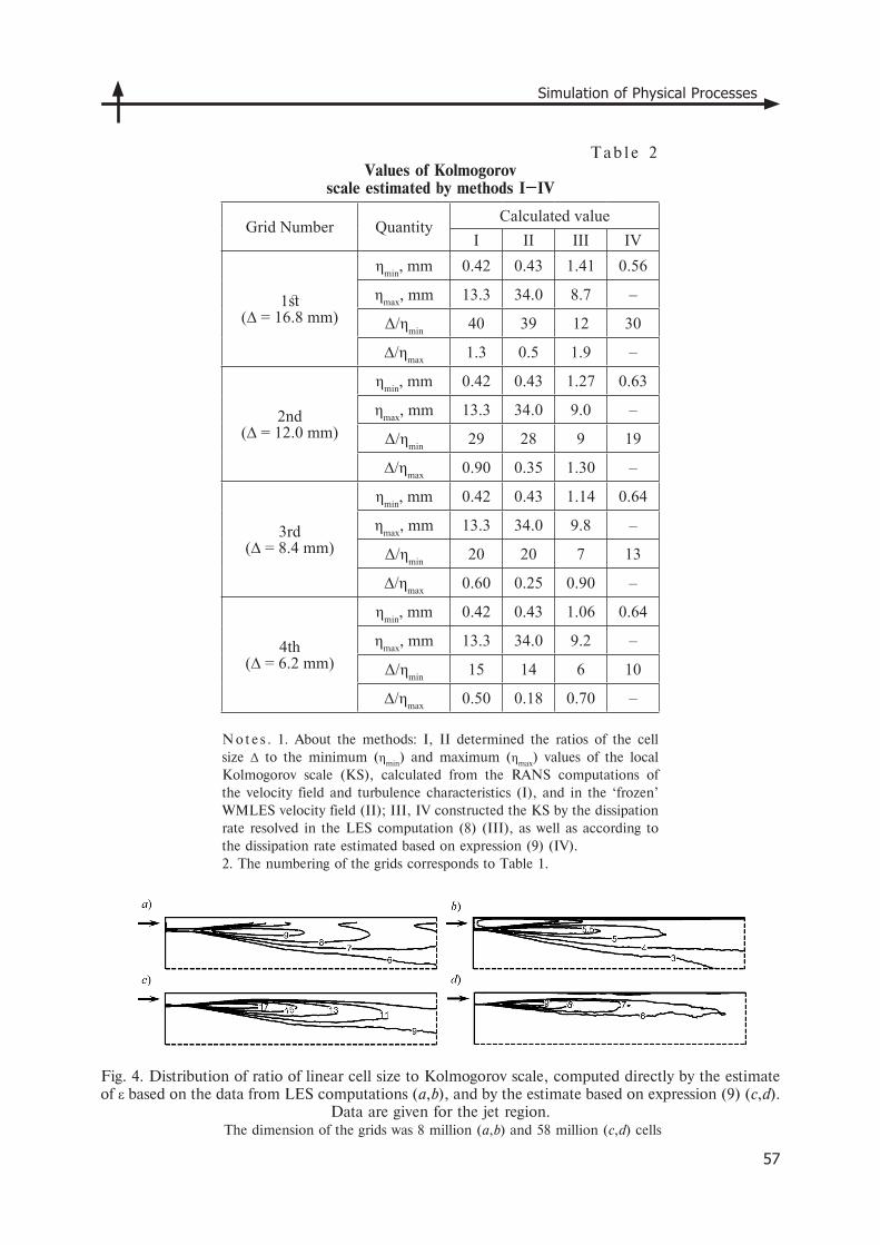
The estimate of η, obtained by directly cal-culating ε using Eq. (8), is illustrated in Fig. 4, a,b, where the isolines correspond to the distri-butions for the ratio of the linear cell size in the grids, consisting of 8 and 58 million cells, to the local values of the Kolmogorov scale. The corresponding minimum values ηmin for differ-ent grids are given in Table 2: the value of the Kolmogorov scale decreases by 33% as the grid is refined from 3 to 58 million cells (the size of cubic elements decreases by almost 3 times).

The dissipation rate of turbulent kinetic en-ergy can be also estimated from the data of LES computations according to the method proposed in [22]; this procedure has already been successfully applied in [23], considering the problem of jet flow. According to the data in [22], instead of directly estimating the value of ε from the LES data, all the other terms in Eq. (7) can be calculated, yielding an indi-rect but more accurate estimate of ε (the sum of all calculated terms should be substituted into equation (6) to find η). The value of the Kolmogorov scale obtained in this way should not change substantially with the change in the dimension of the computational grid.

To estimate η in the mixing layer, it is suf-ficient to calculate only one component in the generation term entering into Eq. (7), which makes the dominant contribution to generating turbulence in this region:

( )' ' .x xy x y x y x

V VV V V V V Vy y

∂ ∂= −

∂ ∂(9)

57


Fig. 4. Distribution of ratio of linear cell size to Kolmogorov scale, computed directly by the estimate of ε based on the data from LES computations (a,b), and by the estimate based on expression (9) (c,d).

Data are given for the jet region. The dimension of the grids was 8 million (a,b) and 58 million (c,d) cells

T ab l e 2Values of Kolmogorov

scale estimated by methods I–IV

Grid Number QuantityCalculated value

I II III IV

1st(∆ = 16.8 mm)

ηmin, mm 0.42 0.43 1.41 0.56

ηmax, mm 13.3 34.0 8.7 –

Δ/ηmin 40 39 12 30

∆/ηmax 1.3 0.5 1.9 –

2nd(∆ = 12.0 mm)

ηmin, mm 0.42 0.43 1.27 0.63

ηmax, mm 13.3 34.0 9.0 –

Δ/ηmin 29 28 9 19

∆/ηmax 0.90 0.35 1.30 –

3rd(∆ = 8.4 mm)

ηmin, mm 0.42 0.43 1.14 0.64

ηmax, mm 13.3 34.0 9.8 –

Δ/ηmin 20 20 7 13

∆/ηmax 0.60 0.25 0.90 –

4th(∆ = 6.2 mm)

ηmin, mm 0.42 0.43 1.06 0.64

ηmax, mm 13.3 34.0 9.2 –

Δ/ηmin 15 14 6 10

∆/ηmax 0.50 0.18 0.70 –

Note s . 1. About the methods: I, II determined the ratios of the cell size Δ to the minimum (ηmin) and maximum (ηmax) values of the local Kolmogorov scale (KS), calculated from the RANS computations of the velocity field and turbulence characteristics (I), and in the ‘frozen’ WMLES velocity field (II); III, IV constructed the KS by the dissipation rate resolved in the LES computation (8) (III), as well as according to the dissipation rate estimated based on expression (9) (IV).2. The numbering of the grids corresponds to Table 1.


58

Calculating term (9) from the data of WMLES computations allowed to obtain one more estimate of ε and, accordingly, the Kolmogorov scale. The distributions of the ra-tios of linear cell sizes in the grids consisting of 8 and 58 million cells to the local values of the field of η computed in this way are shown in Fig. 4, c, d , respectively. The computed min-imum values ηmin for different grids are given in the last column of Table 2: they practically do not vary from grid to grid, tending to ηmin = 0.64 mm as the grid is refined. In this case, a computational grid with the dimension of 51 billion cells is required to carry out valid DNS computations for W/H = 1/6 (306 billion cells for W/H = 1).

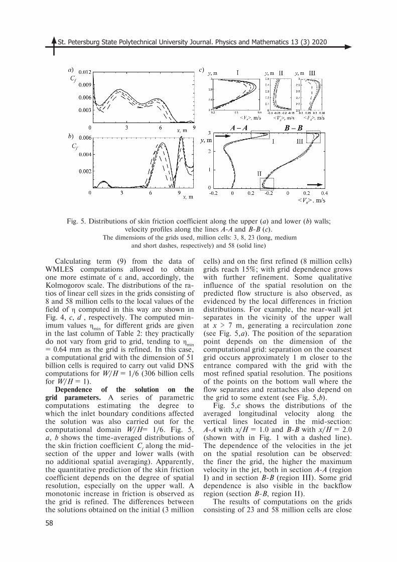
Dependence of the solution on the grid parameters. A series of parametric computations estimating the degree to which the inlet boundary conditions affected the solution was also carried out for the computational domain W/H= 1/6. Fig. 5, a, b shows the time-averaged distributions of the skin friction coefficient Cf along the mid-section of the upper and lower walls (with no additional spatial averaging). Apparently, the quantitative prediction of the skin friction coefficient depends on the degree of spatial resolution, especially on the upper wall. A monotonic increase in friction is observed as the grid is refined. The differences between the solutions obtained on the initial (3 million

cells) and on the first refined (8 million cells) grids reach 15%; with grid dependence grows with further refinement. Some qualitative influence of the spatial resolution on the predicted flow structure is also observed, as evidenced by the local differences in friction distributions. For example, the near-wall jet separates in the vicinity of the upper wall at x > 7 m, generating a recirculation zone (see Fig. 5,a). The position of the separation point depends on the dimension of the computational grid: separation on the coarsest grid occurs approximately 1 m closer to the entrance compared with the grid with the most refined spatial resolution. The positions of the points on the bottom wall where the flow separates and reattaches also depend on the grid to some extent (see Fig. 5,b).

Fig. 5,c shows the distributions of the averaged longitudinal velocity along the vertical lines located in the mid-section: A-A with x/H = 1.0 and B-B with x/H = 2.0 (shown with in Fig. 1 with a dashed line). The dependence of the velocities in the jet on the spatial resolution can be observed: the finer the grid, the higher the maximum velocity in the jet, both in section A-A (region I) and in section B-B (region III). Some grid dependence is also visible in the backflow region (section B-B, region II).

The results of computations on the grids consisting of 23 and 58 million cells are close

Fig. 5. Distributions of skin friction coefficient along the upper (a) and lower (b) walls; velocity profiles along the lines A-A and B-B (c).

The dimensions of the grids used, million cells: 3, 8, 23 (long, medium and short dashes, respectively) and 58 (solid line)

59


to each other both in velocity profiles and in the friction distributions. Thus, the solution can be interpreted as almost grid-independent for a grid with the dimension of 23 million cells. The grid dependence of the solution is more pronounced for cells with a linear size of 12 mm (a grid of 8 million cells); however, it was decided to use these cells with increasing transverse size of the computational domain. If a finer grid with a linear cell size of 8 mm were used in the computations for W/H = 1, it would consist of approximately 140 million cells, which was unacceptable with the available computing resources.

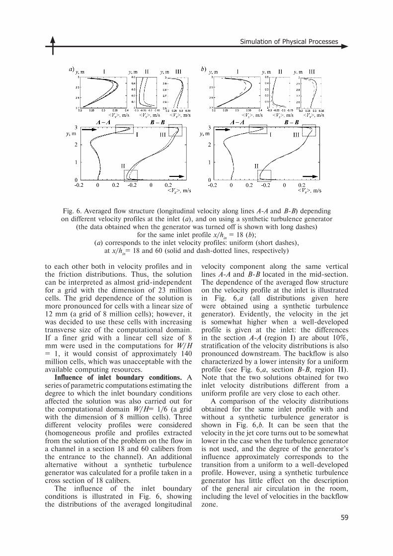
Influence of inlet boundary conditions. A series of parametric computations estimating the degree to which the inlet boundary conditions affected the solution was also carried out for the computational domain W/H= 1/6 (a grid with the dimension of 8 million cells). Three different velocity profiles were considered (homogeneous profile and profiles extracted from the solution of the problem on the flow in a channel in a section 18 and 60 calibers from the entrance to the channel). An additional alternative without a synthetic turbulence generator was calculated for a profile taken in a cross section of 18 calibers.

The influence of the inlet boundary conditions is illustrated in Fig. 6, showing the distributions of the averaged longitudinal

velocity component along the same vertical lines A-A and B-B located in the mid-section. The dependence of the averaged flow structure on the velocity profile at the inlet is illustrated in Fig. 6,a (all distributions given here were obtained using a synthetic turbulence generator). Evidently, the velocity in the jet is somewhat higher when a well-developed profile is given at the inlet: the differences in the section A-A (region I) are about 10%, stratification of the velocity distributions is also pronounced downstream. The backflow is also characterized by a lower intensity for a uniform profile (see Fig. 6,a, section B-B, region II). Note that the two solutions obtained for two inlet velocity distributions different from a uniform profile are very close to each other.

A comparison of the velocity distributions obtained for the same inlet profile with and without a synthetic turbulence generator is shown in Fig. 6,b. It can be seen that the velocity in the jet core turns out to be somewhat lower in the case when the turbulence generator is not used, and the degree of the generator’s influence approximately corresponds to the transition from a uniform to a well-developed profile. However, using a synthetic turbulence generator has little effect on the description of the general air circulation in the room, including the level of velocities in the backflow zone.

Fig. 6. Averaged flow structure (longitudinal velocity along lines A-A and B-B) depending on different velocity profiles at the inlet (a), and on using a synthetic turbulence generator

(the data obtained when the generator was turned off is shown with long dashes) for the same inlet profile x/hin = 18 (b);

(a) corresponds to the inlet velocity profiles: uniform (short dashes), at x/hin= 18 and 60 (solid and dash-dotted lines, respectively)


60

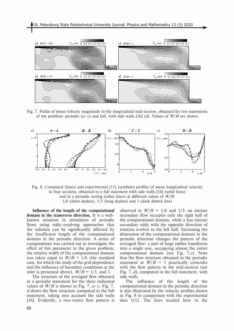
Influence of the length of the computational domain in the transverse direction. It is a well-known situation in simulation of periodic flows using eddy-resolving approaches that the solution can be significantly affected by the insufficient length of the computational domain in the periodic direction. A series of computations was carried out to investigate the effect of this parameter in the given problem; the relative width of the computational domain was taken equal to W/H = 1/6 (the standard case, for which the study of the grid dependence and the influence of boundary conditions at the inlet is presented above), W/H = 1/3, and 1.

The structure of the averaged flow obtained in a periodic statement for the three indicated values of W/H is shown in Fig. 7, a–c; Fig. 7, d shows the flow structure computed in the full statement, taking into account the side walls [16]. Evidently, a two-vortex flow pattern is

observed at W/H = 1/6 and 1/3: an intense secondary flow occupies only the right half of the computational domain, while a less intense secondary eddy with the opposite direction of rotation evolves in the left half. Increasing the dimension of the computational domain in the periodic direction changes the pattern of the averaged flow: a pair of large eddies transforms into a single one, occupying almost the entire computational domain (see Fig. 7,c). Note that the flow structure obtained in the periodic statement at W/H = 1 practically coincides with the flow pattern in the mid-section (see Fig. 7, d), computed in the full statement, with side walls.

The influence of the length of the computational domain in the periodic direction is also illustrated by the velocity profiles shown in Fig. 8 in comparison with the experimental data [11]. The lines located here in the

Fig. 7. Fields of mean velocity magnitude in the longitudinal mid-section, obtained for two statements of the problem: periodic (a–c) and full, with side walls [16] (d). Values of W/H are shown

Fig. 8. Computed (lines) and experimental [11] (symbols) profiles of mean longitudinal velocity in four sections, obtained in a full statement with side walls [16] (solid lines)

and in a periodic setting (other lines) at different values of W/H: 1/6 (short dashes), 1/3 (long dashes) and 1 (dash dotted line)

61


mid-section were shown above by the dashed line in Fig. 1: A-A and B-B are vertical lines; C-C and D-D are horizontal lines with y/H = 0.972 and 0.028, respectively.

It can be seen from Fig. 8 that the profiles obtained for W/H = 1 in the periodic and full statements coincide almost completely. These computations adequately reproduce the flow pattern that was observed experimentally [11] (the quantitative differences between the computational results in the full statement and the experimental data obtained for the backflow region are discussed in [16]). It should be concluded that the flow structure for W/H ≥ 1 is reproduced correctly for the region that is infinite in the z direction. The periodic conditions significantly affect the shape and length of the eddies in the transverse direction for a computational domain of a smaller length, and a certain anisotropy is observed. Eddy structures that are large-scale in the transverse direction are observed at W/H= 1 in the instantaneous fields of SGS viscosity given above (see Fig. 2, c, d). It is impossible to reproduce such eddies in the numerical solution in simulations with a computational domain of a smaller transverse size, which leads to noticeable changes in the averaged fields.

Even though the structure of the averaged flow depends on the size of the computational domain in the standard case with W/H= 1/6, it reflects all the characteristic features of the given flow, namely: the propagation of a near-wall turbulent jet, the development of a mixing layer and the formation of large eddy structures governing the flow as a whole. Thus, the computational results on the influence of the grid and the inlet boundary conditions obtained at W/H= 1/6 can be extended to all of the situations considered.

Conclusion

Eddy-resolving WMLES approach was used in this study for numerical simulation of turbulent air flow in a room ventilated by a 2D air jet supplied from a slit located under the ceiling with the Reynolds number Re = 5·103. The problem was posed in a periodic statement describing a quasi-two-dimensional flow in a room strongly elongated in the transverse direction. The calculations were carried out in the ANSYS Fluent general-purpose CFD code, providing second-order spatial and temporal discretization.

The dependence of the solution on the grid was analyzed in a series of calculations performed on grids with the linear size of a cubic cell ranging from 6 to 16 mm; a baseline grid with a linear cell size of 12 mm was found acceptable. Estimates of the Kolmogorov scale revealed that the minimum values of the Kolmogorov scale in the mixing layer are locally about 20 times smaller than the linear cell size for the standard grid.

We have found that using a synthetic turbulence generator for imposing the inlet boundary conditions has practically no effect on the description of the general air circulation in the room, including the level of velocities in the backflow zone.

We have established that the length of the computational domain in the transverse direction noticeably affects the calculation results if W/H <1. In case of calculations in the region with the length W/H ≥ 1, the averaged structure of a quasi-two-dimensional flow is reproduced correctly in a room elongated in the transverse direction.

The study was supported of the Program for Increasing the Competitiveness of Leading Universities of the Russian Federation (Project 5-100-2020).

REFERENCES

1. Denisikhina D.M., Lukanina M.A., Samoletov M.V., Matematicheskoe modelirovanie microclimata v pomeshchenii basseina [Mathematical modeling of indoor climate in a swimming pool], AВОК: Ventilation, Heating, Air Conditioning, Heat Supply and Building Thermophysics. 6 (2012) 56–61 (in Russian).

2. Palmowska A., Lipska B., Experimental study and numerical prediction of thermal and humidity conditions in the ventilated ice rink arena, Building and Environment. 108 (1 November) (2016) 171–182.

3. Lipska B., Trzeciakiewicz Z., Ferdyn-Grygierek J., Popiolek Z., The improvement of thermal comfort and air quality in the historic assembly hall of a university, Indoor and Built Environment. 21 (2) (2012) 332–337.

4. Niculin D.A., Strelets M.K., Chumakov Yu.S., Rezultaty komputernogo modelirovaniya aerodinamiki i temperaturnogo sostoyaniya interiera Isakievskogo sobora [Results of numerical modelling of the airflow and thermal comfort of St. Isaac’s Cathedral interior], In the sci. collection of articles “Kafedra IV”:


62

«St. Isaac’s Cathedral between the past and the future», Published by St. Isaac’s Cathedral (2008) 404–424 (in Russian).

5. Usachov A.E., Chislennoe issledovanie sistemy ventiliatsii passazhirskogo salona perspectivnogo samoleta [Numerical study of ventilation system of passenger cabin of a perspective aircraft], Scientific Notes of TsAGI, 40 (4) (2009) 56–62 (in Russian).

6. You R., Chen J., Lin C.H., et al., Investigating the impact of gaspers on cabin air quality in commercial airliners with a hybrid turbulence model, Building and Environment. 111 (January) (2017) 110–122.

7. Son C.H., Turner E.H., Smirnov E.M., et al., Integrated computational fluid dynamics carbon dioxide concentration study for the International Space Station, SAE Transactions, Journal of Aerospace. 114 (2005) 89–94.

8. Ivanov N.G., Telnov D.S., Smirnov E.M., Son C.H., Propagation of CO2 field after fire extinguisher discharge: a numerical study, AIAA Techn. Paper AIAA 2011-5078 (2011) 8p.

9. Piomelli U., Large eddy simulations in 2030 and beyond, Phil. Trans. R. Soc. A. 372 (2022) (2014) 20130320.

10. Davidson L., Nielsen P.V. Large eddy simulations of the flow in a three dimensional ventilated room, Proc. of the 5th International Conference on Air Distribution in Rooms ‘ROOMVENT-96’ (Yokohama, Japan, July 17–19, 1996). 2 (1996) 161–168.

11. Nielsen P.V., Restivo A., Whitelaw J.H., The velocity characteristics of ventilated room, J. Fluids Engineering, 100 (3) (1978) 291–298.

12. Jiang Y., Su M., Chen Q., Using large eddy simulation to study airflows in and around buildings, ASHRAE Transactions. 109 (2) (2003) 517–526.

13. Smirnov E.M., Ivanov N.G., Telnov D.S., Son C.H., CFD modeling of cabin air ventilation in the International Space Station: a comparison of RANS and LES data with test measurements for the Columbus Module, Int. J. of Ventilation. 5 (2) (2006) 219–228.

14. Durrani F., Using large eddy simulation to model buoyancy-driven natural ventilation, Ph.D. Thesis, School of Civil and Building Engineering, Loughborough University, UK, 2013.

15. Hawendi S., Gao S., Impact of windward inlet-opening positions on fluctuation characteristics of wind-driven natural cross ventilation in an isolated house using LES, International Journal of Ventilation. 17 (2) (2018) 93–119.

16. Zasimova M.A., Ivanov N.G., Markov D., Numerical modeling of air distribution in a test room with 2D sidewall jet. II. LES-computations for the room with finite width, St. Petersburg Polytechnical State University Journal. Physics and Mathematics. 13 (3) (2020) 65–79.

17. Smagorinsky J., General circulation experiments with the primitive equations. I. The basic experiment, Monthly Weather Review. 91 (3) (1963) 99–164.

18. Shur M.L., Spalart P.R., Strelets M.K., Travin A.K., A hybrid RANS LES approach with delayed-DES and wall-modelled LES capabilities, International Journal of Heat and Fluid Flow. 29 (6) (2008) 1638–1649.

19. Mathey F., Aerodynamic noise simulation of the flow past an airfoil trailing-edge using a hybrid zonal RANS-LES, Computers & Fluids. 37 (7) (2008) 836–843.

20. Sagaut P., Large eddy simulation for incompressible flows: An introduction, 3rd Ed. Springer, Heidelberg (2006).

21. Wilcox D.C., Turbulence modeling for CFD, 3rd Ed., DCW Industries, Inc., La Canada (2006).

22. Dejoan A., Leschziner M.A., Large eddy simulation of a plane turbulent wall jet, Physics of Fluids. 17 (2) (2005) 025102.

23. Guseva E.K., Strelets M.Kh., Travin A.K., et al., Zonal RANS-IDDES and RANS computations of turbulent wake exposed to adverse pressure gradient, Journal of Physics: Conf. Series. 1135, International Conference PhysicA.SPb/2018 23–25 October 2018, Saint Petersburg, Russia (2018) 012092.

Received 20.04.2020, accepted 13.07.2020.

63


THE AUTHORS

ZASIMOVA Marina A.Peter the Great St. Petersburg Polytechnic University29 Politechnicheskaya St., St. Petersburg, 195251, Russian [email protected]

IVANOV Nikolay G.Peter the Great St. Petersburg Polytechnic University29 Politechnicheskaya St., St. Petersburg, 195251, Russian [email protected]

MARKOV Detelin Technical University of Sofia8 Kliment Ohridsky boulevard, Sofia, 1000, [email protected]

СПИСОК ЛИТЕРАТУРЫ

1. Денисихина Д.М., Луканина М.А., Самолетов М.В. Математическое моделирование микроклимата в помещении бассейна // Вентиляция, отопление, кондиционирование воздуха, теплоснабжение и строительная теплофизика (АВОК). 2012. 6. С. 56–61.

2. Palmowska A., Lipska B. Experimental study and numerical prediction of thermal and humid-ity conditions in the ventilated ice rink arena // Building and Environment. 2016. Vol. 108. 1 November. Pp. 171–182.

3. Lipska B., Trzeciakiewicz Z., Ferdyn-Grygierek J., Popiolek Z. The improvement of thermal comfort and air quality in the historic Assembly hall of a university // Indoor and Built Environment. 2012. Vol. 21. No. 2. Pp. 332–337.

4. Никулин Д.А., Стрелец М.Х., Чумаков Ю.С. Результаты компьютерного моделирования аэродинамики и температурного состояния интерьера Исаакиевского собора // Сб. научных трудов «Кафедра IV». Исаакиевский собор между прошлым и будущим. СПб.: Изд-во Исаакиевского собора, 2008. C. 404–424.

5. Усачов А.Е. Численное исследование системы вентиляции пассажирского салона перспективного самолета // Ученые записки ЦАГИ. 2009. Т. XL. 4. С. 56–62.

6. You R., Chen J., Lin C.H., Wei D., Sun H., Chen Q. Investigating the impact of gas-pers on cabin air quality in commercial airlin-ers with a hybrid turbulence model // Building and Environment. 2017. Vol. 111. January. Pp. 110–122.

7. Son C.H., Turner E.H., Smirnov E.M., Ivanov N.G., Telnov D.S. Integrated computational

fluid dynamics carbon dioxide concentration study for the international space station // SAE Transactions. Journal of Aerospace. 2005. Vol. 114. Pp. 89–94.

8. Ivanov N.G., Telnov D.S., Smirnov E.M., Son C.H. Propagation of CO2 field after fire ex-tinguisher discharge: a numerical study // AIAA Techn. Paper AIAA 2011-5078. 2011. 8 p. (https://arc.aiaa.org/doi/abs/10.2514/6.2011-5078)

9. Piomelli U. Large eddy simulations in 2030 and beyond // Phil. Trans. R. Soc. A. 2014. Vol. 372. No. 2022. P. 20130320.

10. Davidson L., Nielsen P.V. Large eddy sim-ulations of the flow in a three dimensional ven-tilated room // Proc. of the 5th International Conference on Air Distribution in Rooms ‘ROOMVENT-96’ (Yokohama, Japan, July 17–19). 1996. Vol. 2. Pp. 161–168.

11. Nielsen P.V., Restivo A., Whitelaw J.H. The velocity characteristics of ventilated room // J. Fluids Engineering. 1978. Vol. 100. No. 3. Pp. 291–298.

12. Jiang Y., Su M., Chen Q. Using large eddy simulation to study airflows in and around build-ings // ASHRAE Transactions. 2003. Vol. 109. No. 2. Pp. 517–526.

13. Smirnov E.M., Ivanov N.G., Telnov D.S., Son C.H. CFD modeling of cabin air ventilation in the International Space Station: a comparison of RANS and LES data with test measurements for the Columbus Module // International Journal of Ventilation. 2006. Vol. 5. No. 2. Pp. 219–228.

14. Durrani F. Using large eddy simulation to model buoyancy-driven natural ventila-tion. School of Civil and Building Engineering, Loughborough University, UK. 2013. Ph.D. Thesis. 187 p.


64

© Peter the Great St. Petersburg Polytechnic University, 2020

15. Hawendi S., Gao S. Impact of windward inlet-opening positions on fluctuation charac-teristics of wind-driven natural cross ventilation in an isolated house using LES // International Journal of Ventilation. 2018. Vol. 17. No. 2. Pp. 93–119.

16. Засимова М.А., Иванов Н.Г., Марков Д. Численное моделирование циркуляции воздуха в помещении при подаче из плоской щели. II. LES-расчеты для помещения конечной ширины // Научно-технические ведомости CПбГПУ. Физико-математические науки, 2020, 3. С. 56–74.

17. Smagorinsky J. General circulation exper-iments with the primitive equations. I. The basic experiment // Monthly Weather Review. 1963. Vol. 91. No. 3. Pp. 99–164.

18. Shur M.L., Spalart P.R., Strelets M.K., Travin A.K. A hybrid RANS-LES approach with delayed-DES and wall-modelled LES capabilities // International Journal of Heat and Fluid Flow.

2008. Vol. 29. No. 6. Pp. 1638–1649.19. Mathey F. Aerodynamic noise simulation

of the flow past an airfoil trailing-edge using a hybrid zonal RANS-LES // Computers & Fluids. 2008. Vol. 37. No. 7. Pp. 836–843.

20. Sagaut P. Large Eddy Simulation for in-compressible flows: An introduction. 3rd Ed. Heidelberg: Springer, 2006. 556 p.

21. Wilcox D.C. Turbulence modeling for CFD. 3rd Ed. La Canada: DCW Industries, Inc., 2006. 515 p.

22. Dejoan A., Leschziner M.A. Large eddy simulation of a plane turbulent wall jet // Physics of Fluids. 2005. Vol. 17. No. 2. P. 025102.

23. Guseva E.K., Strelets M.Kh., Travin A.K., Burnazzi M., Knopp T. Zonal RANS-IDDES and RANS computations of turbulent wake exposed to adverse pressure gradient // Journal of Physics: Conf. Series. 2018. Vol. 1135. International Conference PhysicA.SPb/2018 23–25 October 2018, Saint Petersburg, Russia. P. 012092.

Статья поступила в редакцию 20.04.2020, принята к публикации 13.07.2020.

СВЕДЕНИЯ ОБ АВТОРАХ

ЗАСИМОВА Марина Александровна – ассистент Высшей школы прикладной математики и вычислительной физики Санкт-Петербургского политехнического университета Петра Великого, Санкт-Петербург, Российская Федерация.

195251, Российская Федерация, г. Санкт-Петербург, Политехническая ул., [email protected]

ИВАНОВ Николай Георгиевич – кандидат физико-математических наук, доцент Высшей школы прикладной математики и вычислительной физики Санкт-Петербургского политехниче-ского университета Петра Великого, Санкт-Петербург, Российская Федерация.

195251, Российская Федерация, г. Санкт-Петербург, Политехническая ул., [email protected]

МАРКОВ Детелин – PhD, доцент Софийского технического университета, г. София, Болгария.1000, Болгария, г. София, бульвар Климента Орхидского, [email protected]

Documents

NUMERICAL MODELING OF AIR DISTRIBUTION IN A TEST ROOM …