Embed Size (px)
Citation preview

Numerical modeling of geomechanical processes related to CO2 injection within generic
reservoirs
Final Scientific/Technical Report: DE-FE0001836
PI: Andreas Eckert
On behalf of
Missouri University of Science and Technology
1870 Miner Circle, Rolla, MO 65409
Project period: December 2009 to May 2013
Rolla, August 12, 2013
DISCLAIMER
“This report was prepared as an account of work sponsored by an agency of the United States
Government. Neither the United States Government nor any agency thereof, nor any of their
employees, makes any warranty, express or implied, or assumes any legal liability or
responsibility for the accuracy, completeness, or usefulness of any information, apparatus,
product, or process disclosed, or represents that its use would not infringe privately owned rights.
Reference herein to any specific commercial product, process, or service by trade name,
trademark, manufacturer, or otherwise does not necessarily constitute or imply its endorsement,
recommendation, or favoring by the United States Government or any agency thereof. The
views and opinions of authors expressed herein do not necessarily state or reflect those of the
United States Government or any agency thereof.”
ABSTRACT
In this project generic anticline structures have been used for numerical modeling analyses to
study the influence of geometrical parameters, fluid flow boundary conditions, in situ stress
regime and inter-bedding friction coefficient on geomechanical risks such as fracture reactivation
and fracture generation. The resulting stress states for these structures are also used to determine
safe drilling directions and a methodology for wellbore trajection optimization is developed that
is applicable for non-Andersonian stress states.
The results of the fluid flow simulation show that the type of fluid flow boundary condition is of
utmost importance and has significant impact on all injection related parameters. It is
recommended that further research is conducted to establish a method to quantify the fluid flow
boundary conditions for injection applications.
The results of the geomechanical simulation show that in situ stress regime is a crucial, if not the
most important, factor determining geomechanical risks. For extension and strike slip stress
regimes anticline structures should be favored over horizontally layered basin as they feature
higher ΔPc magnitudes. If sedimentary basins are tectonically relaxed and their state of stress is
characterized by the uni-axial strain model the basin is in exact frictional equilibrium and fluids
should not be injected. The results also show that low inter bedding friction coefficients
effectively decouple layers resulting in lower ΔPc magnitudes, especially for the compressional
stress regime.
Table of Contents
1. Reservoir Scale Model ............................................................................................................. 9
1.1. Fluid Flow Simulation ...................................................................................................... 9
1.1.1. Introduction ............................................................................................................... 9
1.1.2. Modeling Approach ................................................................................................ 10
1.1.3. Model Description .................................................................................................. 12
1.1.4. Results ..................................................................................................................... 14
1.1.4.1. Effect of Wavelength Variation ....................................................................... 15
1.1.4.2. Effect of Reservoir Layer Thickness Variation ............................................... 16
1.1.4.3. Effect of Amplitude Variation ......................................................................... 16
1.1.4.4. Simultaneous variation of Wavelength, Amplitude and Height ...................... 17
1.1.4.5. Effect of Boundary Conditions ........................................................................ 18
1.1.4.6. Effect of Depth ................................................................................................ 19
1.1.5. Discussion ............................................................................................................... 20
1.1.6. Conclusions ............................................................................................................. 23
1.2. Geomechanical Analysis ................................................................................................ 24
1.2.1. Introduction ............................................................................................................. 24
1.2.2. Modeling Approach ................................................................................................ 26
1.2.3. Finite Element Model ............................................................................................. 27
1.2.3.1. Geometry and Boundary Conditions ............................................................... 27
1.2.3.2. Pore Pressure – Stress Coupling ...................................................................... 28
1.2.3.3. Results ............................................................................................................. 28
1.2.4. Coupled Model........................................................................................................ 31
1.2.4.1. Model Setup and Boundary Conditions ........................................................... 31
1.2.4.2. Results ............................................................................................................. 33
1.2.4.2.1. Compressional Stress Regime ...................................................................... 34
1.2.4.2.2. Extensional Stress Regime ........................................................................... 43
1.2.4.2.3. Strike Slip Stress Regime ............................................................................. 55
1.2.5. Discussion ............................................................................................................... 66
1.2.6. Conclusions ............................................................................................................. 70
2. Wellbore Scale Model ........................................................................................................... 71
2.1. Model Initialization ....................................................................................................... 71
2.1.1. Introduction ............................................................................................................. 71
2.1.2. Theoretical Background .......................................................................................... 72
2.1.3. Geomechanical Model and Input Data ................................................................... 76
2.1.4. Modeling Approach ................................................................................................ 77
2.1.5. Results ..................................................................................................................... 78
2.1.5.1. Displacement Boundary Conditions ................................................................ 78
2.1.5.2. Mesh Optimization .......................................................................................... 84
2.1.5.3. Stress Boundary Conditions and Drilling Simulation Boundary Conditions .. 85
2.1.6. Discussion ............................................................................................................... 88
2.1.6.1. Models Using the Displacement Boundary Conditions .................................. 88
2.1.6.2. Comparisons of the Models for the Different Boundary Conditions .............. 90
2.1.6.3. Implications for Safe Mud Weight Prediction ................................................. 90
2.1.7. Conclusions ............................................................................................................. 93
2.2. Wellbore Stability Analysis .......................................................................................... 94
2.2.1. Pressure Window .................................................................................................... 94
2.2.2. Vertical Wellbores .................................................................................................. 94
2.2.3. Deviated Wellbores ................................................................................................. 97
2.2.4. Wellbore Stresses for Arbitrary Well Orientations ................................................. 98
2.2.5. Wellbore Stability Analysis: Setup ....................................................................... 100

2.2.6. Wellbore Stability Analysis: Model Validation .................................................... 103
2.2.7. Wellbore Stability Analysis: Stress Regimes ....................................................... 105
2.2.7.1. Extensional Stress Regime ............................................................................ 105
2.2.7.2. Compressional Stress Regime ....................................................................... 107
2.2.7.3. Strike-Slip Regime ........................................................................................ 109
2.2.7.4. Influence of inter bedding friction ................................................................. 111
2.2.8. Conclusions ........................................................................................................... 113
2.3. Wellbore Trajectory Optimization .............................................................................. 113
2.3.1. Introduction ........................................................................................................... 113
2.3.2. Theoretical Background ........................................................................................ 115
2.3.2.1. Stress in the Subsurface ................................................................................. 115
2.3.2.2. Failure Criteria and Safe Mud Pressure ......................................................... 115
2.3.3. Application ............................................................................................................ 116
2.3.3.1. Surface Location Fixed .................................................................................. 117
2.3.3.2. Surface Location Flexible .............................................................................. 119
2.3.4. Results of the Case Study ..................................................................................... 120
2.3.5. Summary And Conclusions .................................................................................. 125
3. Overall Concluding Remarks and Accomplishments .......................................................... 126
EXECUTIVE SUMMARY
Preventing environmental damages from CO2 release into the atmosphere, underground storage
of liquefied CO2 has become a goal in recent research projects. The successful sequestration of
the CO2 depends on minimizing the risk of leakage through cap rock and fracture networks.
Assessment of cap rock stability, fracture generation and reactivation due to injection related
pore pressure increase as well as wellbore integrity thus becomes of major interest and successful
modeling of these parameters will help to find suitable conditions for possible CO2 sequestration
sites. The main objective of this ARRA training project was to properly train graduate students to
develop multi-scale Finite Element (FE) models of different geological settings for sequestration
sites and compare the results concerning geomechanical processes, such as how fluid pressure
induces rock deformation, as well as critical wellbore placement and wellbore integrity to each
other. This shall give a more thorough understanding of how reservoir geometry affects wellbore
stability, formation and cap rock stability and thus shall facilitate future site selection.
In order to analyze and evaluate these geomechanical risks the numerical modeling methods
employed in this project focus on two different spatial scales. 1) the reservoir system scale to
study fluid flow boundary conditions and geometrical influences of anticline structures on the
state of stress and to analyze the risk of fracture generation and reactivation and 2) the borehole
scale system to determine stable drilling directions and wellbore trajectory optimization. The
numerical models employed in this project focus on generic anticline structures as these geologic
scenarios represent prime targets for CO2 sequestration sites. It is important to note that the
results showcase the relative importance of the modeling parameters investigated and the
methodology developed can readily be applied to real case scenarios.
The fluid flow simulation on the reservoir scale investigates the influence of geometrical
parameters such as wavelength, amplitude and thickness as well as the influence of the fluid flow
boundary conditions on safe injection limits. The results show that higher wavelengths, lower
amplitudes and relatively thick layers provide the best conditions for safe CO2 sequestration. A
major and not surprising conclusion is that the lateral fluid flow boundary condition of an aquifer
system has the most significant influence on the CO2 sequestration parameters. The assumption
of an open system requires gigantic aquifers (~100 km) that may be very difficult, if not
impossible, to locate in the vicinity of many CO2 producers. A more realistic approach of semi-
open fluid flow boundaries yields similar if not better results than the open system case.
However, this approach seems only applicable if the total magnitude of the lateral flow boundary
condition of an aquifer system can be determined e.g. by water drawdown tests similar to
conventional pressure transient testing and production data analysis of the oil and gas wells. Our
results show that for such a system, the anticline wavelength, amplitude and thickness have a
pronounced influence on CO2 sequestration parameters. However, unless extensive field tests
permit the application of semi-open or open aquifer, this study shows that the safest approach for
a sustainable CO2 sequestration project should be the assumption of closed fluid flow
boundaries.
On the reservoir scale a 3D finite element (FE) model is employed to assess maximum
sustainable pore pressures prior to injection. The FE results of the stress state are used for
analytical estimates based on the pore pressure - stress coupling principle. Based on these
estimates the strike-slip regime results in the highest sustainable pore pressure differences. The
generic anticline geometries investigated in this study have also shown that in addition to the in-
situ state of stress the stress heterogeneities associated to the geometry of such structures result
in significant differences with respect to sustainable pore pressure magnitudes (ΔPc). For
extension and strike slip stress regimes anticline structures should be favored over horizontally
layered basin as they feature higher ΔPc magnitudes. If sedimentary basins are tectonically
relaxed and their state of stress is characterized by the uni-axial strain model the basin is in exact
frictional equilibrium and fluids should not be injected.
The analytical pre-injection estimates together with the coupled simulations have shown and
confirmed that the in-situ stress regime is a crucial, if not the most important, factor determining
geomechanical risks, for fluid injection applications such as CO2 sequestration. It is therefore
strongly recommended that every case study is based on in-situ stress measurements for a
thorough calibration of numerical models used to analyze geomechanical risks. The coupled
simulations for the generic anticline structures have shown that the extensional stress regime
represents the overall safest scenario, however is considered the most unlikely as anticlines are
compressional structures.
Another important observation from the generic models is the influence of geological parameters
such as the inter-bedding friction coefficient. Whilst the influence of this parameter is not
important for horizontally layered structures, the geometry of anticline structures results in stress
heterogeneities and the coefficient of friction on bedding planes determines the mechanical
coupling between different layers. The results have shown that low friction coefficients
effectively decouple layers resulting in lower ΔPc magnitudes, especially for the compressional
stress regime.
On the borehole scale a methodology has been established to setup and optimize numerical
models in order to minimize errors. The results of the FE models on the reservoir scale have been
used to perform a wellbore stability analysis and to find stable drilling directions for the anticline
structures. While vertical wells have proven to be stable for all three stress regimes, a procedure
has been developed that can be readily applied to prospective case studies with more complex
material models and geometries. The procedure developed provides mud pressure window
calculation for inclined wellbores of type I wells. These wellbore types, especially type I
wellbores with a horizontal hold section, are relevant for CO2 sequestration applications, as
horizontal wells have an increased surface area inside the reservoir and thus feature increased
injectivity. As predicted by Kirsch’s analytical solution the in-situ stress regime has significant
impact on stable drilling directions, whereby the direction of the intermediate principal stress
represents the least stable direction. This procedure developed becomes of relevance when
applied to case studies where the principal stresses are not given by V, and h,H. In order to
further improve the resulting wellbore stability analysis a wellbore trajectory optimization
procedure is necessary to account for scenarios where the vertical stress is not a principal stress.
The methodology developed represents a process to optimize wellbore trajectories in the
planning stage of a well. Assumptions on the state of stress are not necessary as the 3D FEM
provides the complete stress tensor at any point in the model. The methodology is based on the
general mathematical description and thus enables all possible scenarios of azimuth, inclination
and surface rig location for multiple well types along the entire trajectory of the well path. The
case study results show that if applied to a scenario with a highly varying state of stress a
significant improvement of wellbore stability conditions can be achieved. In comparison to a
vertical well the proposed well trajectory has a significantly wider mud pressure window also
resulting in a reduction of casing points.

1. Reservoir Scale Model
For the reservoir scale models of the generic anticline structures 3 different analyses have been
performed:
a) Fluid Flow Simulation
b) Geomechanical Analysis:
a. Pre-injection Geomechanical Assessment of Maximum Sustainable Pore
Pressures
b. Coupled Analysis
1.1.Fluid Flow Simulation
1.1.1. Introduction
Often numerical CO2 injection scenarios are based on the simplified assumption of a
horizontally layered sedimentary basin [Settari and Mourits, 1998; Thomas et al., 2003; Dean et
al., 2006; Pettersen, 2006; Zhou et al., 2008; Inoue, 2009; Taberner et al., 2009; Tran et al.,
2009; Ehlig-Economides And Economides, 2010; Cappa and Rutqvist, 2011; Graupner et al.,
2011]. While this scenario serves well to study the impact of different parameters (such as
permeability, injection rate, fluid flow boundary conditions and seal efficiency) on CO2 flow and
pressurization [Zhou et al., 2008; Inoue, 2009; Taberner et al., 2009; Ehlig-Economides And
Economides, 2010; Cappa and Rutqvist, 2011], for a geomechanical risk analysis a model
geometry reflecting the actual geologic scenario, which exhibits a heterogeneous state of stress is
required. The geomechanical risks accompanying aquifer pressurization due to the CO2 injection
have been investigated by several authors [Settari and Mourits, 1998; Thomas et al., 2003;
Pettersen, 2006; Van der Meer et al., 2006; Rutqvist et al., 2007; Schembre-McCabe et al., 2007;
Zhou et al., 2008; Inoue, 2009; Taberner et al., 2009; Tran et al., 2009; Ehlig-Economides And
Economides, 2010; Cappa and Rutqvist, 2011; Graupner et al., 2011] with one of the most
important being the reactivation of existing faults or fracture sets which can result in induced
seismicity [Van der Meer et al., 2006; Rutqvist et al., 2007; Schembre-McCabe et al.,
2007;Loizzo et al., 2009] and potential leakage pathways. [Rutqvist et al., 2007; Zhou et al.,
2008] have shown that the pressure build-up in models representing horizontally layered
sedimentary basins is strongly dependent, amongst others, on the fluid flow boundary conditions.
A closed system, reflecting a compartmentalized reservoir, results in a much higher and faster
pressure increase than open-flow boundary conditions. This influence of the fluid flow boundary
conditions on the pressure build-up becomes increasingly relevant for geomechanical risk
analyses of storage sites exhibiting a heterogeneous state of stress [Paradeis et al., 2012].
Possible geologic scenarios may represent an aquifer being trapped in a closed system bounded
by faults or an anticline structure which may have existing fracture sets along the hinge.
Anticline/Antiform structures as an example of folded sedimentary layers are among the most
common structural traps for hydrocarbon reservoirs and thus become a prime target of the
emerging challenge of safe geologic sequestration of CO2 [Metz et al., 2005].
One reason for the utilization of simple geometries for generic fluid flow simulation studies is
due to the lack of flexible pre-processors, which can generate finite difference grids of more
complex geometries. Preprocessors for the finite element method have the ability to generate
complex structures but do not yield discretization formats which can be used in finite difference
based reservoir simulations [Amirlatifi et al., 2011a; Amirlatifi et al., 2011b]. In this paper we
address this limitation by using a commercial finite element pre-processor (Altair®
Hypermesh®) and use the Coupled Geomechanical Reservoir Simulator, CGRS, a coupling
module for geomechanical reservoir simulation developed at Missouri University of Science and
Technology [Amirlatifi et al., 2011a; Amirlatifi et al., 2011b] to convert several synthetic
reservoir geometries from the finite element file format to the reservoir simulation grid file
format. We then study the effects of anticline geometry on CO2 injection parameters. We use the
commercial fluid flow simulation package Schlumberger® Eclipse® to investigate the effects of
different amplitudes, wavelengths and height of generic anticline structures on the storability of
CO2 in these reservoirs at different depths and under different injection rates. The results of this
study may finally serve as a guideline for possible injection sites and scenarios resembling the
cases presented here. The methodology presented in this paper further enables coupling between
the reservoir simulation and the geomechanical analysis whereby both simulations use the same
discretization minimizing the use of interpolation algorithms.
1.1.2. Modeling Approach
Numerical modeling studies in the oil and gas industry assume a realistic reservoir geometry
which is obtained by seismic data, well logs and surface mapping. The data collection may result
in quite complex reservoir geometries. Although most state of the art commercial simulators are
capable of handling unstructured grids that can accommodate these complex structural features,
the computational cost of aforementioned simulators limits their applicability. This feature is not
commonly employed and finite difference discretization is still the prominent practice. However,
the limitation of finite difference discretization algorithms [Amirlatifi et al., 2011a; Amirlatifi et
al., 2011b] for reservoir simulation studies requires up-scaling and simplification of the complex
geometry. As a result, most of the preprocessors in the oil and gas industry are based on
discretizing an existing geometry and it is very difficult, if not impossible, to use them for
building parametric study models that incorporate anticlines, for example. This limitation has
resulted in the implementation of simplified horizontal basin models in most of the literature,
unless real field data are present. As part of our efforts to couple the finite element (FE) analysis
package Abaqus® with Eclipse® in the Coupled Geomechanical Reservoir Simulator, CGRS,
we have created a file convertor and grid mapper in Java® that converts geometries created in
the Abaqus 3D file format to the grid file format of Eclipse®. The FE pre-processor Altair®
Hypermesh® is used to generate 3D anticline models of different amplitude, wavelengths and
heights. Due to the requirements of finite difference grids, all grid blocks in the 3D FE model
need to be hexahedral in columns sharing the same coordinates in horizontal directions albeit
variable depth. Once the geometry is created in the FEA preprocessor, it is exported to the
Abaqus® 3D file format and is transferred into the CGRS file convertor. The initial step of the
file conversion routine stores the nodal coordinates and the corresponding elements into the
memory and organizes them into arrays of nodes and elements. In the next step, the nodes are
sorted by their coordinates and the closest node to the origin is selected as the starting point of
the finite difference grid. The nodes are then sorted by their X-coordinates for an initial constant
y-coordinate. Once all nodes having the same Y-coordinates are identified, the next row in the Y
direction is examined and so forth, until all elements and nodes in the first layer are determined
and the process continues with the elements and nodes in the second and the following layers (z-
coordinates). At each step, the number of rows, columns and layers are determined as the
maximum number of nodes in any row, column and layer. Once all nodes and elements in the
finite element mesh are analyzed, the corresponding Eclipse® grid is generated. The coordinates
of the nodes in the first layer are reported by the COORD keyword in the generated Eclipse®
grid data file, followed by the vertical location of each node, reported under the ZCORN
keyword. This efficient method enables us to generate highly flexible generic geometries for
reservoir simulation studies with the ease of finite element analysis pre-processors.
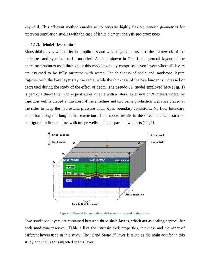
1.1.3. Model Description
Sinusoidal curves with different amplitudes and wavelengths are used as the framework of the
anticlines and synclines to be modeled. As it is shown in Fig. 1, the general layout of the
anticline structures used throughout this modeling study comprises seven layers where all layers
are assumed to be fully saturated with water. The thickness of shale and sandstone layers
together with the base layer stay the same, while the thickness of the overburden is increased or
decreased during the study of the effect of depth. The pseudo 3D model employed here (Fig. 1)
is part of a direct line CO2 sequestration scheme with a lateral extension of 76 meters where the
injection well is placed at the crest of the anticline and two brine production wells are placed at
the sides to keep the hydrostatic pressure under open boundary conditions. No flow boundary
condition along the longitudinal extension of the model results in the direct line sequestration
configuration flow regime, with image wells acting as parallel well sets (Fig.1).
Figure 1: General layout of the anticline structure used in this study.
Two sandstone layers are contained between three shale layers, which act as sealing caprock for
each sandstone reservoir. Table 1 lists the intrinsic rock properties, thickness and the order of
different layers used in this study. The “Sand Stone 2” layer is taken as the main aquifer in this
study and the CO2 is injected in this layer.
Table 1. Properties of layers used in the parametric study.
Layer Name ρ
(Kg/m3)
E
(MPa)
ν (%) k
(10-16
m2)
Sw (%)
Overburden 2210 1500 0.25 0.01 0.098 100
Shale 1 2130 1500 0.25 0.01 0.0009 100
Sand Stone 1 2210 2000 0.25 20 986.9 100
Shale 2 2130 1500 0.25 0.01 0.0009 100
Sand Stone 2 2210 2000 0.25 20 986.9 100
Shale 3 2130 1500 0.25 0.01 0.0009 100
Base 2245 1500 0.25 0.01 0.098 100
Table 2 lists the range of geometrical and operational parameters that were used in this study.
Wavelengths of 750, 1500 and 3000 meters and an infinite wavelength, resembling the
horizontally layered basin are used (section 2.4). Reservoir thicknesses of 25, 50 and 100 meters
are considered (section 2.5). In order to investigate effect of amplitude variation, anticlines with
amplitudes of 50, 100 and 150 meters are modeled (section 2.6). The simultaneous variation of
wavelength, thickness and amplitude is examined as described in section 2.7 and Table 7. Effect
of boundary condition is examined through modeling of the closed, Semi-Open and Open
boundary conditions as described in section 2.8. Depth of the model is varied between 500 to
3000 meters as described in section 2.9 which has resulted in different maximum allowable pore
pressures. The lateral extent of the model is varied between 6, 23 and 103 Km as described in the
discussion. As a reference base case of this study we consider a reservoir at the depth of 1250
meters with an anticline of a wavelength of 1500 m, an amplitude of 150 m and a height of 100
meters. The injection well is located at the crest of the anticline and the boundaries are assumed
to be closed. In order to evaluate the validity of the simplified horizontally layered basin models,
a simple horizontally layered basin model is created and is compared to the base model.
Simulations reflecting open boundary fluid flow conditions are carried out by placing water
production wells at the boundaries that maintain hydrostatic pore pressure. An initial CO2
injection rate of 20.7 KTons/year (1798.71 lbs/MWhr) is based on the 50% reinjection of CO2
emission rate of a common 495 MW capacity coal fired power plant [18] with 75% efficiency
over 100 years period and CO2 density of 1.98 Kg/m3 and formation properties are based on the
geology of common sedimentary rocks.
Table 2: Range of parameters used in the parametric study.
Units
Values
Attribute
Depth m 500 1000 1250 1500 2000 2500 3000
Maximum Allowable Pore
Pressure MPa 26.3 34.1 36.0 41.8 49.5 56.5 62.4
Wave Length m 1500 750
Amplitude m 150 100 50
Reservoir Thickness m 100 50 25
Well Location Crest
Boundary Type Open Closed
Injection Rate m3/sec 0.33194
Model Size Km 3 23 103
Number of Anticlines 0 1 3
Table 3: The base simulation case and its simulation results.
Attribute Units Value
Anticline Wavelength m 1500
Anticline Amplitude m 150
Anticline Height m 100
Depth m 1250
Reservoir Volume m3 9129120
Boundary Closed
CO2 Injection Rate m3/sec 0.33194
Fault Present No
Well Location Crest of Anticline
Number of Anticlines 1
Critical Pore Pressure MPa 36.0
Safe Injection Limit Years 6.35
CO2 Saturation at SIL % 53
Average Pressure at SIL MPa 32.45
Mass of Injected CO2 103Tons 117.583
Occupancy % 1.62
1.1.4. Results
For the injection simulations we use a maximum allowable pore pressure before failure of intact
rock is initiated as a threshold value before injection is stopped. These critical pore pressure
values are determined by geomechanical finite element analysis for each geometry assuming a
compressional stress regime, as described in [Rutqvist et al., 2007; Paradeis et al., 2012]. Based
on these results the reservoir simulation analyses are conducted, thus a one way coupling
procedure is followed here. Simulations results are checked on a monthly basis until the pore
pressure in any grid block of the reservoir layer or the surrounding shale layers reaches the
maximum allowable pore pressure. The time to reach the maximum allowable pore pressure is
identified as the Safe Injection Limit, SIL. The ratio of the reservoir volume of CO2 at the SIL to
the total pore volume, which is also equal to the average gas saturation, is considered as the
degree of occupancy, an indication of how well the reservoir volume is utilized. Unless
maximum allowable pore pressure is reached, the simulation is continued for 50 years. The
simulation results of the base anticline model of this study, Fig. 1 and Table 3, are taken as the
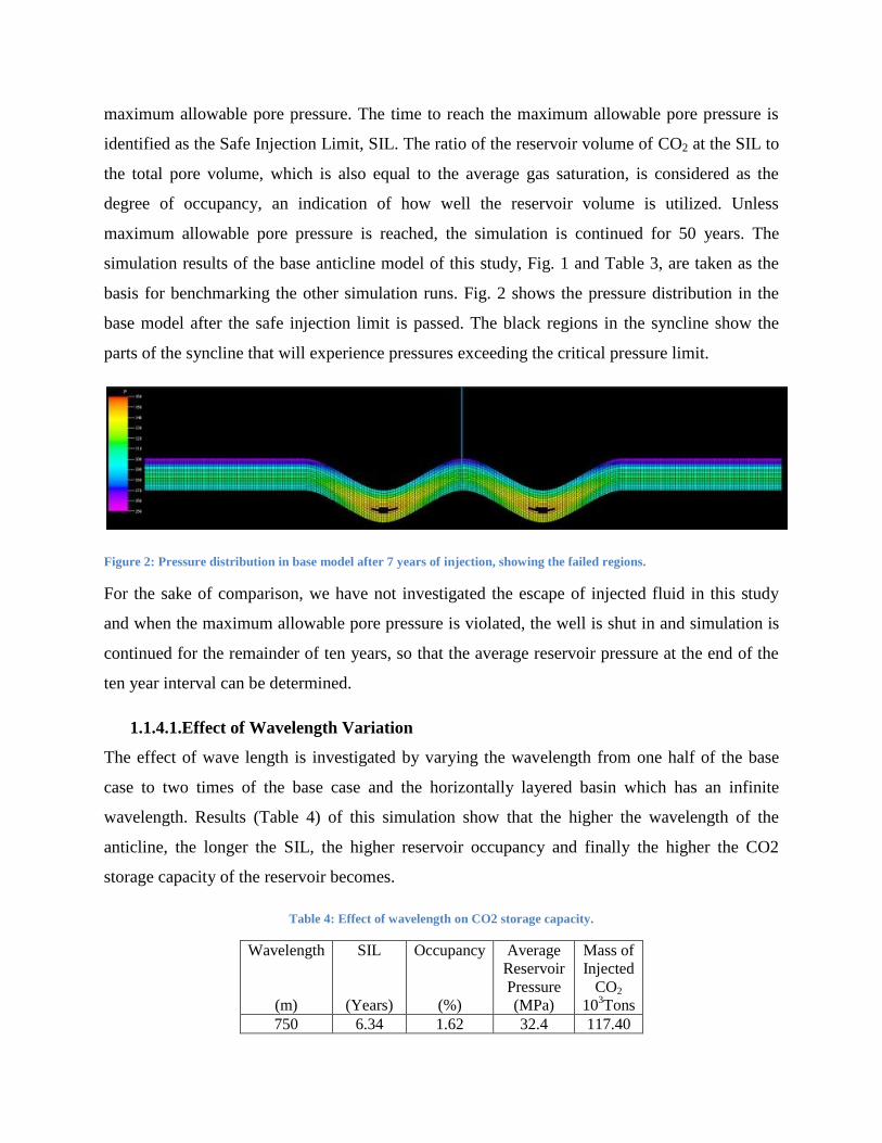
basis for benchmarking the other simulation runs. Fig. 2 shows the pressure distribution in the
base model after the safe injection limit is passed. The black regions in the syncline show the
parts of the syncline that will experience pressures exceeding the critical pressure limit.
Figure 2: Pressure distribution in base model after 7 years of injection, showing the failed regions.
For the sake of comparison, we have not investigated the escape of injected fluid in this study
and when the maximum allowable pore pressure is violated, the well is shut in and simulation is
continued for the remainder of ten years, so that the average reservoir pressure at the end of the
ten year interval can be determined.
1.1.4.1.Effect of Wavelength Variation
The effect of wave length is investigated by varying the wavelength from one half of the base
case to two times of the base case and the horizontally layered basin which has an infinite
wavelength. Results (Table 4) of this simulation show that the higher the wavelength of the
anticline, the longer the SIL, the higher reservoir occupancy and finally the higher the CO2
storage capacity of the reservoir becomes.
Table 4: Effect of wavelength on CO2 storage capacity.
Wavelength
(m)
SIL
(Years)
Occupancy
(%)
Average
Reservoir
Pressure
(MPa)
Mass of
Injected
CO2
103Tons
750 6.34 1.62 32.4 117.40
1500 6.35 1.62 32.5 117.58
3000 7.15 1.79 34.8 132.54
∞ 7.80 1.93 35.1 144.59
1.1.4.2.Effect of Reservoir Layer Thickness Variation
The reservoir height directly controls CO2 storage capacity through variation of accessible pore
volume. Eq. (1) shows the pore volume for a simple case of a cubic reservoir of constant height,
h, porosity, , and area, A.
"V=Ah∅" (1)
An immediate conclusion from Eq. (1) is that the higher the reservoir thickness, the more pore
space is available for CO2 sequestration, assuming that we have a connected pore network. Table
5 shows the effect of variation in height on the CO2 storage capacity on the base model.
Table 5: Effect of height on CO2 storage capacity.
Height
(m)
SIL
(Years)
Occupancy
(%)
Average
Reservoir
Pressure
(MPa)
Mass of
Injected
CO2
103Tons
25 1.65 1.6 31.8 30.56
50 3.29 1.6 32.5 60.95
100 6.35 1.6 32.4 117.58
The simulation results confirm that the increased volume of the reservoir results in increased safe
injection limits and consequently an increase in injected gas volume is achieved, but the overall
occupancy stays the same.
1.1.4.3.Effect of Amplitude Variation
Three different amplitude variations of the base case, presented in Table 3, are considered,
ranging from 50 meters to 150 meters in the closed system. The simulation results of such
variations are presented in Table 6.
Table 6: Effect of amplitude on CO2 storage capacity.
Amplitude
(m)
SIL
(Years)
Occupancy
(%)
Average
Reservoir
Pressure
(MPa)
Mass of
Injected
CO2
103Tons

50 7.32 1.83 34.2 135.56
100 6.82 1.72 33.3 126.39
150 6.35 1.62 32.4 117.58
As the results suggest, the lower amplitude anticline gives the highest CO2 storage capacity of
135.56 kilo Tons. Assuming that the most favorable case is to increase the average reservoir
pressure up to the maximum allowable pore pressure, an anticline with the low amplitude of 50
meters yields the best average reservoir pressure of 34.2 MPa.
1.1.4.4.Simultaneous variation of Wavelength, Amplitude and Height
Simultaneous variation of wavelength, amplitude and reservoir height are studied through 15
simulations where the wavelength is varied between 750 meters and 1500 meters, the amplitude
is varied between 50 meters, 100 meters and 150 meters and the height is varied between 25
meters, 50 meters and 100 meters. Results of these simulations are presented in Table 7.
Table 7: Simultaneous variation of wavelength, amplitude and height.
Wavelength
(m)
Amplitude
(m)
Height
(m)
SIL
(Years)
Occupancy
(%)
Mass of Injected
CO2
103Tons
750 50
25 1.81 1.75 32.54
50 3.71 1.84 68.14
100 7.23 1.82 134.66
100
25 1.73 1.67 30.92
50 3.46 1.73 63.46
100 6.82 1.74 126.93
1500 50
25 1.9 1.82 33.98
50 3.79 1.87 69.58
100 7.32 1.83 136.10
100
25 1.73 1.68 30.92
50 3.57 1.76 64.90
100 6.82 1.72 126.93
150
25 1.65 1.6 30.56
50 3.29 1.65 60.95
100 6.35 1.62 117.58
The results show that the highest storage capacity is observed for the high wavelength of 1500
meters, the low amplitude of 50 meters and the thick reservoir of 100 meters thickness. As
previously shown in Table 5 and confirmed in Table 7, height or net thickness of the reservoir
has a direct effect on the CO2 storage capacity.
1.1.4.5.Effect of Boundary Conditions
Three types of fluid flow boundary conditions can be thought for the aquifer systems, namely
Open, Semi-Open and Closed boundaries [Ehlig-Economides and Economides, 2010; Zhou et
al., 2008]. Many scholars have assumed fully open boundaries where the pressure at the
boundary remains hydrostatic. These studies show very promising results on the storage capacity
and the safety of the project. We have considered 3 cases where storage under open boundary
condition is compared to the closed and semi-open boundaries. In order to simulate open
boundary conditions per definition, two brine production wells are placed at the sides of the
aquifer and the constraints are set such that the well flowing pressure, Pwf, remains at the
hydrostatic pore pressure. The limit for the injection period is set equal to the CO2 breakthrough
time. In the semi-open model, the production rate of the brine producers is reduced by half and
the pressure is allowed to increase at the boundaries until the safe sequestration pressure limit is
reached, or until the CO2 breaks through the production wells, which was the case here. Table 8
presents the simulation results of the base case under different boundary conditions.
Table 8: Effect of Boundary Conditions on CO2 Storage Capacity of the base case.
Boundary
Type
SIL
(Years)
Occupancy
(%)
Average
Reservoir
Pressure
(MPa)
Mass of Injected
CO2
103Tons
Closed 6.35 1.62 32.4 117.58
Open 50 25.13 13.1 942.10
Semi-
Open 80 25.96 20.4 1506.65
The results show the significant influence of the fluid flow boundary condition. Whilst a Closed
system (resembling a compartmentalized reservoir) yields a SIL of only 6.35 years and an
occupancy of only 1.62%, Open and Semi-Open systems yield much higher SIL (50-80 years)
and much higher occupancies (25-26%). The Semi-Open system yields overall safer conditions
and more CO2 can be injected by allowing partial pressure increase in the reservoir, resulting in
compression of CO2 and contained spread of the plume. The contained spreading gives higher
sweep efficiency and continuous flow of fluids in the system, which itself results in increased
contact between the two fluids and dissolution of CO2 in the brine. While open systems benefit
from the favorable pressure gradient that makes it possible for CO2 to quickly spread in the
system, mix with the brine as it spreads and dissolve in it, unconstrained spreading of the plume
results in lower sweep efficiency than that of the Semi-Open system.

1.1.4.6.Effect of Depth
The depth of the reservoir determines the state of the stress, the resulting maximum allowable
pore pressure as well as the CO2 density and phase (Fig. 3), which in turn determines its
compressibility and viscosity. The resulting effects on CO2 storage capacity are studied through
7 simulations where the depth of the base case, as described in Table 3, is varied from 500
meters to 3000 meters. A compressional stress regime is assumed for the calculation of the
maximum allowable pore pressure. Table 9 presents the simulation results for the base case at
different depths.
Table 9: Effect of Depth variation on CO2 Storage Limit.
Reservoir Depth
(m)
Maximum Allowable
Pore Pressure (MPa)
SIL
(Years)
Occupancy
(%)
Mass of Injected CO2
103Tons
500 26.3 5.266 1.57 97.45
1000 34.1 6.28 1.60 116.41
1250 36.0 6.35 1.62 117.58
1500 41.8 7.73 1.88 143.86
2000 49.5 8.877 2.04 165.52
2500 56.5 9.619 2.13 179.44
3000 62.4 9.78 2.10 182.53
The results show that CO2 sequestration in deep formations results in longer safe CO2 injection
periods and consequently higher CO2 storage capacity. The highest occupancy is observed in
2500 meters depth with a value of 2.13% and the deepest model at a depth of 3000 meters has
the longest injection period of 9.78 years. Comparison between the increase in injection period
and the increase in depth and the occupancy suggests that 2500 meters is the most favorable
depth of all cases under closed boundary conditions.
Figure 3: Phase Diagram of CO2.
1.1.5. Discussion
CO2 sequestration based fluid flow simulations utilizing simplified horizontally layered basins
show promising results regarding the amount of CO2 that can be safely injected over long
periods of time [Zhou et al., 2008; Birkholzer et al., 2009]. The assumption of a horizontally
layered basin, however, neglects the requirement of a structural trap system to store the fluids. A
prime example of such trap systems are anticline structures. The results presented in this study
show that once realistic structural geometries for CO2 sequestration projects are considered,
geometrical parameters such as anticline wavelength, anticline amplitude and respective aquifer
depth influence the SIL, the occupancy and the total amount of injected CO2.The results
presented in Table 4, Table 6 & Table 7 suggest that the anticline wavelength and amplitude
have direct influence on the CO2 storage capacity. The larger the wavelength and the lower the
amplitude, the longer it takes to get to the maximum allowable pore pressure in a closed system
and thus the more CO2 can be injected into the anticline. Comparison with the horizontally
layered basin shows that the horizontally layered basins have more storage capacity than the
actual capacity of an anticline structure. This suggests that the existence of anticline structures
should not be ignored by simplifying the model with horizontally layered basins. Using
simplified model geometries can result in the prediction of Safe Injection Limits that are longer
than the actual tolerance of the medium. When comparing the influence of the geometrical
parameters on the CO2 occupancy in closed systems, the results only show slight variations.
However, once other fluid flow boundary conditions are considered the effects of the geometrical
parameters become significantly more pronounced. Table 10 shows the effect of reservoir height
and boundary condition variation on CO2 storage capacity.
Table 10: Effect of reservoir height and boundary condition variation on CO2 storage capacity
Height
(m)
Boundary
Type
SIL
(Years)
Occupancy
(%)
Average
Reservoir
Pressure
(MPa)
Mass of Injected
CO2
103Tons
50 Closed 3.29 1.65 32.1 60.95
Open 30.72 28.95 13.9 577.13
100 Closed 6.35 1.62 32.4 117.58
Open 50 25.13 13.1 942.10

Although the occupancy of the two models in a closed system is the same, the thinner reservoir
of 50 meter thickness shows a better sweep and occupancy of 28.95% under the open conditions,
compared to the 25.13% of the 100 meter thick reservoir. While the difference in the volume of
the two reservoirs controls the mass of injected CO2 and SIL, the difference in occupancy can
show the influence of geometrical parameters that may be masked out otherwise by the influence
of the fluid flow boundary conditions.
The simulation results confirm previous studies [Ehlig-Economides and Economides, 2010;
Zhou et al., 2008] showing that the type of fluid flow boundary condition has a huge impact on
the result parameters. CO2occupancy in closed systems is a function of total compressibility.
When more pore space is available, assuming that the total compressibility stays the same, more
CO2 volume can be injected into the reservoir, but the overall occupancy of the reservoir stays
the same regardless of the volume or the height, as shown in Table 5. Our results of maximum
occupancy of 1.6%-2% compare well with results from [Zhou et al., 2008] of 0.5% and [Ehlig-
Economides and Economides, 2010] of ~1% for closed systems.
The effect of the lateral fluid flow boundary conditions on CO2 storage capacity for the base
anticline was presented in Table 8. These results suggest that the assumption of open boundary
condition can significantly increase the CO2 storage capacity but a semi-open boundary serves
the purpose even better, as long as the pressure stays in the safe injection limit. The question,
however, is whether the open boundary condition case can be observed in real life. One way of
achieving open boundary conditions is through the use of pore volume multipliers [Samier et al.,
2007] which, in the authors’ opinion, are only applicable to reservoir simulation studies, where
exact knowledge about the size and water flux of the aquifer is not available. Under these
circumstances one may use the pore volume multipliers on the aquifer grid blocks to achieve a
history match. However, this is not the case in studies concerning CO2 sequestration in saline
formations where the aquifer is the most important part of the fluid system. Another way of
achieving open boundary conditions, as presented previously, is to drill brine production wells at
the boundaries and control the pressure through these production wells. While drilling of these
wells is possible, a question that needs to be addressed is where to dispose of the produced brine.
Another possibility is to have such large aquifers that the compressibility of the liquids in place
doesn’t result in the increased pore pressure. In order to investigate the typical size needed for
such an aquifer, we have made two extensions of the base case where the boundaries are
extended 10km and 50km on each side of the 3km wide anticline structure, resulting in reservoirs
that are 23 and 103 km long respectively. As it is shown in Table 11, the large reservoir of 23 km
width fails to replicate the results of the fully open boundary and the gigantic reservoir of 103km
size is the minimum reservoir size capable of replicating such results. This conclusion leaves us
with some fundamental questions that need to be answered before one can make the fully open
boundaries assumption:
1. What is the likelihood of finding such gigantic reservoirs in the immediate vicinity of
CO2 producers?
2. Provided that such a reservoir is available, are there any faults/inhomogenities or stress
anomalies that influence the maximum allowable pore pressure?
3. What is the probability that no one else is injecting in the same aquifer of interest which
would otherwise result in pressure interference in the premises of the well(s) that are
planned for the CO2 sequestration?
Table 11: Comparison of Different Model Sizes and Boundary Conditions.
Reservoir Size
(km)
Reservoir Volume
(106m)
SIL
(Years)
Boundary Type Mass of Injected CO2
103Tons
6 9.13 6.35 Closed 117.58
6 9.13 50 Open 942.11
23 35.0 22.46 Closed 420.71
103 156.7 50 Closed 942.10
The presented results show that the lateral fluid flow boundary conditions have a significant
influence on CO2 sequestration parameters. Although huge aquifers such as Sleipner
[Kongsjorden et al., 1998] exist throughout the world that have high potential for CO2
sequestration, they may not be in the vicinity of the power plant(s) of interest or meet the salinity
level requirements set forward by federal or state regulations; thus an important step in CO2
sequestration feasibility study of a candidate aquifer should be determination of its size. This can
be achieved by analogy between the existing and well established practices in petroleum
engineering for well testing and estimation of the size/drainage radius of an oil well. Without
knowing the exact size of the aquifer and matching boundary type, care should be taken before
suggesting safe sequestration limits. In the authors’ opinion, it is better to take the more
conservative practice and assume semi-open or closed boundaries to stay within the safe
sequestration limit, instead of assuming that the aquifer has fully open boundaries and face the
otherwise high risk of exceeding the maximum allowable pore pressure and causing the rock to
fail. Note should be taken that the maximum allowable pore pressure used throughout this study
is the pressure that will result in failure of intact rock, which is obviously greater than the critical
pore pressure needed for reactivation of favorably oriented existing failed structures.
1.1.6. Conclusions
While the assumption of using horizontally layered basins for CO2 sequestration studies may be
valid for most cases, the need for an actual trap system requires a more realistic geometry for
parametric studies and simulations. The geometry should be flexible enough to include faults or
fractures and any unconformities that may exist. Our study shows that by using finite element
analysis pre-processor geometries resembling structural trap systems can be generated and
successfully converted into native fluid flow simulation formats. This novel approach enables us
to study the influence of geometric parameters such as anticline wavelength, amplitude and
thickness.
The results of our study show that higher wavelengths, lower amplitudes and relatively thick
layers provide the best conditions for safe CO2 sequestration. Further, the depth of the
sequestration site also plays an important role. Our results conclude that for aquifer depths of
2500m and 3000m (for a closed system) the maximum occupancy and SIL can be obtained,
respectively. If the economic costs of drilling to the deeper aquifers and compression of CO2 for
injection into such reservoirs can be justified, deep CO2 sequestration results in higher storage
capacity.
A major and not surprising conclusion is that the lateral fluid flow boundary condition of an
aquifer system has the most significant influence on the CO2 sequestration parameters. The
assumption of an open system requires gigantic aquifers (~100 km) that may be very difficult, if
not impossible, to locate in the vicinity of many CO2 producers. The open system assumption
might also lead to over-simplified cases, unless brine production wells are included. A more
realistic approach of semi-open fluid flow boundaries yields similar if not better results than the
open system case. However, this approach seems only applicable if the total magnitude of the
lateral flow boundary condition of an aquifer system can be determined e.g. by water drawdown
tests similar to conventional pressure transient testing and production data analysis of the oil and
gas wells. Our results show that for such a system, the anticline wavelength, amplitude and
thickness have a pronounced influence on CO2 sequestration parameters. However, unless
extensive field tests permit the application of semi-open or open aquifer, this study shows that
the safest approach for a sustainable CO2 sequestration project should be the assumption of
closed fluid flow boundaries.
1.2.Geomechanical Analysis
1.2.1. Introduction
Geologic CO2 sequestration in deep saline aquifers, depleted oil and gas fields and unmineable
coal seams has been identified as a possibility to reduce CO2 emissions from coal fired power
plants and production facilities (Metz et al., 2007), provided that a thorough understanding of the
storage site is conducted. The selection of suitable injection sites depends critically on the
assessment of geomechanical risks such as fracture reactivation associated to the pore pressure
increase (e.g. Streit and Hillis, 2004; Li et al., 2006; Rutquist et al., 2007; Rutquist et al., 2008;
Vidal-Gilbert et al., 2009; Cappa and Rutqvist, 2011). Sibson (2003) shows that hydraulic
extensional fractures are only critical for intact rock at low differential stress and that the
reactivation of cohesion-less, optimally oriented shear fractures determines the lower limit of
sustainable reservoir overpressures. These fractures, if critically stressed, represent fluid flow
pathways (Barton et al., 1995) along which dissolved CO2 may escape into the atmosphere or
into freshwater aquifers. If such fractures are reactivated due to fluid injection applications
induced seismicity with moment magnitudes ranging from -3 to 5 can be observed (e.g. Gibbs et
al., 1973; Wesson and Nicholson, 1987; Cappa and Rutquist, 2011; Verdon et al., 2011). In order
to assess these geomechanical risks a thorough understanding of the state of stress at potential
sequestration sites is necessary.
Numerical simulations provide excellent tools for a critical assessment of reservoir
pressurization and the associated geomechanical risks. A thorough and most realistic
representation of the in-situ effective stress conditions requires the coupling of a fluid flow
simulation through porous media with a geoemchanical analysis (e.g. Settari and Mouritis, 1998;
Rutqvist et al., 2002; Dean et al., 2006; Vidal-Gilbert et al., 2009). As a major conclusion from

such studies, the prevailing stress regime (Rutqvist et al., 2007; Rutqvist et al., 2008; Paradeis et
al., 2012) and the fluid flow boundary conditions (Zhou et al., 2008; Rutqvist et al., 2007) are the
most critical parameters. Often such numerical modeling studies of CO2 injection scenarios are
simplified to a horizontally layered sedimentary basin (Li et al., 2006; Rutquist et al., 2007;
Rutquist et al., 2008; Zhou et al., 2008; Cappa and Rutqvist, 2011). These simplified model
geometries are valuable to study the influence of parameters such as permeability, injection rate,
fluid flow boundary conditions and seal efficiency on CO2 plume spreading and pressurization
(e.g. Zhou et al., 2008; Inoue, 2009; Taberner et al., 2009; Ehlig-Economides and Economides,
2010; Cappa and Rutqvist, 2011). A geomechanical risk assessment simulating an accurate
representation of the often heterogeneous in-situ state of stress requires model geometries
reflecting the actual geologic scenario and thus considering the mechanical contribution arising
from geometrical heterogeneities (Rutqvist et al., 2008; Amirlatifi et al., 2012; Paradeis et al.,
2012). In this regard anticline structures are among the most common structural traps for
hydrocarbon reservoirs and thus become a prime target of the emerging challenge of safe
geologic sequestration of CO2 (Metz et al., 2007). CO2 sequestration in anticline structures has
been investigated by Paradeis et al. (2012) and Amirlatifi et al. (2012). Amirlatifi et al. (2012)
perform a fluid flow simulation analysis based on generic anticline geometries and show that low
amplitude, large wavelength anticline structures provide the best conditions for CO2
sequestration. They also conclude that the fluid flow boundary conditions are of utmost
importance when evaluating geomechanical risks due to fluid injection. Paradeis et al. (2012)
utilize the same generic model geometries and perform a finite element based pre-injection risk
assessment by calculating the critical pore pressure increase based on the geometrical factors of
anticline wavelength and amplitude and the prevailing stress regime. Using a simplified
analytical solution neglecting pore pressure - stress coupling they conclude that the stress regime
is the most critical factor and that for extensional and strike slip stress regimes anticline
structures provide safer conditions than horizontally layered basins.
In this paper the generic anticline model geometries used in Paradeis et al. (2012) and Amirlatifi
et al. (2012) are used to further evaluate critical geologic parameters and to perform a pseudo-3D
coupled geomechanical analysis to assess the fault reactivation risk within generic anticline
structures. Of particular interest in this study is the coefficient of friction between bedding layers
and its impact on critical sustainable pore pressures and the resulting risk of fault reactivation.
Flexural slip between sedimentary layers accommodates the strain during multi-layer folding and
it has been shown that the presence or absence of interlayer slip strongly controls the distribution
and evolution of strain within folded strata (Smart et al., 2009) and thus has a significant impact
on fracture reactivation (Sanz et al., 2008; Smart et al., 2009). The coefficient of friction between
bedding planes effectively describes the coupling between different layers, whereby a low
coefficient of friction represents a weak coupling and a high competence contrast between
adjacent layers is produced (Twiss and Moores, 2002). A large coefficient of friction represents a
strong coupling and hence different friction values should result in different stress and strain
distributions across adjacent bedding layers.
In order to study the influence of the inter-bedding coefficient of friction for extensional, strike-
slip and compressional stress regimes this study first presents a pre-injection geomechanical risk
assessment based on simplified analytical solutions including the pore pressure - stress coupling
effect (Altmann et al., 2010) and then the results of a pseudo-3D partially coupled fluid flow -
geomechanical analysis are presented to show the interplay of friction coefficient and stress
regime and their influence on fault reactivation probability and the safe injection limits within
anticline structures.
1.2.2. Modeling Approach
The numerical modeling analysis comprises a finite element analysis based on the prevailing
stress regime that is used for a pre-injection assessment of critical sustainable pore pressures, and
a partially coupled fluid flow - geomechanical analysis for analysis of the CO2 injection related
risk of fracture reactivation for different stress regimes and inter-bedding friction coefficients.
It is important to note that the modeling approach is based on the assumption that the anticline
structure is pre-existing and that static displacement boundary conditions can be used to simulate
the different far-field stress regimes. The modeling approach does not consider the structural
development of the anticline over geologic time scales. Different geologic strain rates result in
different states of stress of an anticline. However, this represents an extensive sensitivity study
by itself which was outside the scope of this paper. A static state of stress using displacement
boundary conditions is considered sufficient to enable the study of the model parameters of the
anticline and represents the most common approach to simulate in-situ stress states for
geomechanical studies.
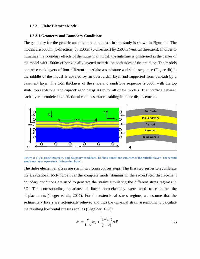
1.2.3. Finite Element Model
1.2.3.1.Geometry and Boundary Conditions
The geometry for the generic anticline structures used in this study is shown in Figure 4a. The
models are 6000m (x-direction) by 1500m (y-direction) by 2500m (vertical direction). In order to
minimize the boundary effects of the numerical model, the anticline is positioned in the center of
the model with 1500m of horizontally layered material on both sides of the anticline. The models
comprise rock layers of four different materials: a sandstone and shale sequence (Figure 4b) in
the middle of the model is covered by an overburden layer and supported from beneath by a
basement layer. The total thickness of the shale and sandstone sequence is 500m with the top
shale, top sandstone, and caprock each being 100m for all of the models. The interface between
each layer is modeled as a frictional contact surface enabling in-plane displacements.
Figure 4: a) FE model geometry and boundary conditions. b) Shale-sandstone sequence of the anticline layer. The second
sandstone layer represents the injection layer.
The finite element analyses are run in two consecutives steps. The first step serves to equilibrate
the gravitational body force over the complete model domain. In the second step displacement
boundary conditions are used to generate the strains simulating the different stress regimes in
3D. The corresponding equations of linear poro-elasticity were used to calculate the
displacements (Jaeger et al., 2007). For the extensional stress regime, we assume that the
sedimentary layers are tectonically relieved and thus the uni-axial strain assumption to calculate
the resulting horizontal stresses applies (Engelder, 1993).
(1 2 )
1 (1 )h V P
(2)
For strike-slip and compressional regimes, the three-dimensional boundary conditions are
calculated using the relative stress ratios. For both of these regimes, the vertical stress is given by
the integration of overburden density. In a strike-slip regime, the minimum principle stress is the
minimum horizontal stress which is given by , the vertical stress is the intermediate
principle stress and the maximum principle stress is . For the compressional regime,
the vertical stress is the minimum principle stress, the intermediate stress is and the
maximum principle stress is .
1.2.3.2.Pore Pressure – Stress Coupling
Simplified analytical techniques can be used as a pre-injection risk estimate for fault reactivation.
The principle of pore pressure – stress coupling (Engelder and Fischer, 1994; Hillis, 2001) can
be used to estimate the maximum sustainable pore pressure, Pc, (e.g. Wiprut and Zoback, 2000;
Streit and Hillis, 2004; Rutqvist et al., 2008) for sites where limited geological knowledge exists.
Pore pressure – stress coupling is based on the observation that the total minimum horizontal
stress changes with a change in pore pressure (Teufel et al., 1991). However, as recent studies by
Mueller et al. (2010) and Altmann et al. (2010) show, pore pressure stress coupling does not only
affect the minimum horizontal stress but affects all components of the principal stress tensor and
is a complex function of space and time. Altmann (2010) shows that pore pressure stress
coupling is therefore different for each stress regime. For the pre-injection risk assessment the
principle of pore pressure - stress coupling, based on the long term limits given by Altmann et al.
(2010), is utilized to determine the maximum sustainable pore pressure, Pc, for fault reactivation
in extensional, strike-slip and compressional stress regimes. The simplification to the long term
limits becomes especially relevant for subsurface engineering applications such as CO2
sequestrations which are interested in how much pore pressure change is sustainable over long
times. The following simplified analytical solutions are based on the Mohr Coulomb failure
criterion and the detailed derivations for these equations can be found in the Appendix.
1.2.3.3.Results
As the state of stress in an anticline displays the largest variations on a vertical cross section at
the crest of the structure (Paradeis et al., 2012), for the determination of the maximum
sustainable pore pressure, Pc, the stress changes associated to pore pressure – stress coupling
along the V-direction are considered for the various stress regimes. Assuming a friction
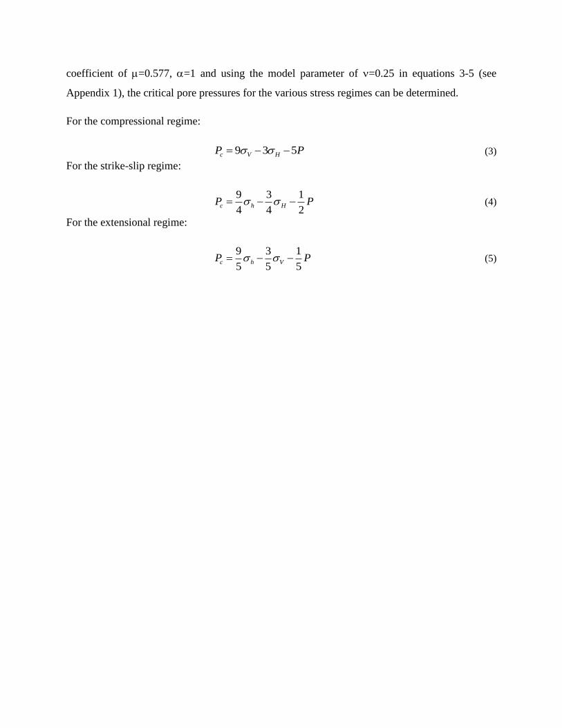
coefficient of =0.577, =1 and using the model parameter of =0.25 in equations 3-5 (see
Appendix 1), the critical pore pressures for the various stress regimes can be determined.
For the compressional regime:
9 3 5c V HP P (3)
For the strike-slip regime:
9 3 1
4 4 2c h HP P (4)
For the extensional regime:
9 3 1
5 5 5c h VP P (5)
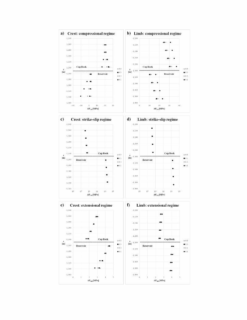
Figure 5: Critical pore pressure difference for the various stress regimes at the crest and limb of the anticline structure.
For the compressional stress regime the cap rock can sustain higher ΔPc magnitudes than the reservoir layer. Fo the
extensional and strike-slip regime the cap rock is able to sustain lower ΔPc magnitudes than the reservoir layer and seal
integrity (in terms of the permeability contrast) is more crucial.
Using equations 3, 4, and 5 the maximum sustainable pore pressure change, ΔPc=Pc-P,
based on the initial effective state of stress can be calculated for the various stress regimes.
Figure 5a-f show ΔPc along the vertical direction for the reservoir and cap rock layers. For each
stress regime the coefficient of friction between the bedding planes is given values of =0.1, 0.3,
0.5 and 0.8 to study the influence of inter-bedding coupling.
The results show that for the compressional stress regime in the reservoir layer ΔPc is close to 0
MPa and fracture reactivation is very likely. However, across the interface to the cap rock ΔPc
increases to 16.4 MPa for m=0.1 and 25.8 MPa for m=0.8. As Figure 5a shows, higher friction
coefficients result in a higher sustainable pore pressure across the interface.
For the strike-slip stress regime (Figure 5c) ΔPc is slightly higher with 23.2 MPa in the reservoir
layer than in the cap rock (18.6 MPa). The influence of the inter-layer friction coefficient is
minimized as the vertical stress is a principal stress included in equation (4).
For the extensional stress regime (Figure 5e) displays the overall lowest critical pore pressure
magnitudes of ~4.5 MPa in the reservoir layer and 1.5-2 MPa in the cap rock. Hereby, lower
friction coefficients result in lower ΔPc magnitudes in the cap rock. The extensional stress
regime shows how critical the seal integrity (in terms of permeability) is.
1.2.4. Coupled Model
1.2.4.1.Model Setup and Boundary Conditions
The realistic assessment of the geomechanical risks due to CO2 injection related pore pressure
increases requires the utilization of a modeling approach that that involves multiphase and multi-
component fluid flow in a geologic system. The study of mechanical deformations under such
conditions is achieved by numerical modeling of fluid flow through porous medium coupled
with a geomechanical analysis of the medium at different pore pressure distributions (Rutqvist et
al., 2002; Settari and Mourits, 1998; Settari and Walters, 1999; Thomas et al., 2003; Vidal-
Gilbert et al., 2009). For this purpose an implicit partially coupled fluid flow-geomechanical

analysis coupling ECLIPSETM
and ABAQUSTM
developed at Missouri S&T (Amirlatifi et al.,
2011a,b; project: DE-FE0001132) is utilized. Amirlatifi et al.’s (2012) coupling approach
enables coupling between the reservoir simulation and the geomechanical analysis whereby both
simulations use the same discretization minimizing the use of interpolation algorithms.
The pseudo 3D model employed here is part of a direct line CO2 sequestration scheme with a
lateral extension of 76 meters where the injection well is placed at the crest of the anticline. No
flow boundary condition along the longitudinal extension of the model results in the direct line
sequestration configuration flow regime, with image wells acting as parallel well sets (Figure 6).
A CO2 injection well is placed at the crest of the anticline in the bottom reservoir layer. The well
is perforated all the way in the reservoir layer. The lateral fluid flow boundary conditions reflect
a closed system. Furthermore, the simulations are based on 1 year injection time-steps to
minimize computational costs. The relevant simulation and injection parameters are given by
Table 12.
Figure 6: Model geometry and CO2 injection setup as a direct line scheme with image wells. In order to utilize partially
coupled modeling approach for the anticline models the model geometry of Figure x has been slightly altered. Instead of
1500m in the y-direction the model dimension had to be decreased to 76m. The reduction of the model dimension in y-
direction is due to the computational requirements of the coupling procedure. Due to license availability the simulation
had to be run on a high performance desktop PC. Larger model dimensions would have increased the simulation time
manifold without producing significantly different results.
Table 12: Boundary Conditions and model paramters
Parameter Units Assumed values
Stress Regimes [ ] Extensional
Compressional

Strike Slip
Coefficient of Friction(μ) [ ] 0.1
0.8
Well Location [ ] Crest
Boundary type [ ] Closed
CO2 Injection rate (STD) kTons/Year 20 (28680 m3/day)
Reservoir Thickness m 100
Wavelength m 1500
Amplitude m 100
FP: cohesion [MPa] 15
FP: friction angle deg 33
FP: tensile strength [MPa] 7.5
1.2.4.2.Results
Note: Due to licensing problems for the reservoir simulation software ECLIPSE at Missouri
S&T, during the project period, only the results for fracture generation can be presented.
In order to show the occurrence of fault generation due to the CO2 related pore pressure increase
this study utilizes the concept of Fracture Potential (Eckert and Connolly, 2007; Verdon et al.,
2010). Fracture Potential (FP) describes the ratio between the actual differential stress and the
differential stress at failure, and thus, if FP=1 can be used to indicate regions in a numerical
model where fault generation occurs. The concept of Fracture Potential to assess the likelihood
of fracture occurrence is chosen to overcome convergence problems of the numerical models
once appropriate plasticity models are applied in ABAQUSTM
. Whilst such plasticity models are
a standard procedure and can be readily included, a coupled effective stress – displacement
analysis including contact surfaces has resulted in severe convergence problems and stable
solutions could not be obtained. As a suitable alternative solution, FP represents a post-
processing failure criterion which is automatically calculated after each time iteration modeled.
The various CO2 injection scenarios are halted when the FP in the cap rock reaches 1 and the
achieved injection time is termed Safe Injection Limit (SIL). For the various stress regimes, CO2
injection scenarios are analyzed for inter-bedding friction coefficients of 0.1. and 0.8.
Before the CO2 injection stages an in initial hydrostatic pore pressure distribution is applied
throughout the model as shown in Figure 7.

Figure 7 - Hydrostatic Pore Pressure Distribution in bar in the model.
1.2.4.2.1. Compressional Stress Regime
For the compressional regime in this study, the vertical stress is the minimum principle stress,
the intermediate stress is given by and the maximum principle stress is given by
.
Figure 8 and Figure 9 show the initial shear fracture potential for the anticline with the
coefficient of friction of 0.1 and 0.8 between the layers under the compressional regime
respectively.

Figure 8 - Initial Shear Fracture Potential - Coefficient of friction = 0.1 – Compressional Model
Figure 9 - Initial Shear Fracture Potential - Coefficient of friction = 0.8 – Compressional Model
As shown in these two figures, the initial shear fracture potential in the two models is similar in
the overburden and base of the model, but the two models behave differently in the shale-sand
layers. While the μ=0.8 model is initially at an elevated FP state, compared to the μ=0.1 model, it
is speculated that this model will tolerate the increase in pore pressure better, since the
differential stresses occurring across model layers is reduced.
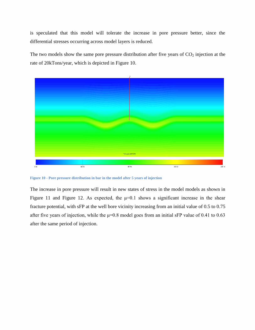
The two models show the same pore pressure distribution after five years of CO2 injection at the
rate of 20kTons/year, which is depicted in Figure 10.
Figure 10 - Pore pressure distribution in bar in the model after 5 years of injection
The increase in pore pressure will result in new states of stress in the model models as shown in
Figure 11 and Figure 12. As expected, the μ=0.1 shows a significant increase in the shear
fracture potential, with sFP at the well bore vicinity increasing from an initial value of 0.5 to 0.75
after five years of injection, while the μ=0.8 model goes from an initial sFP value of 0.41 to 0.63
after the same period of injection.
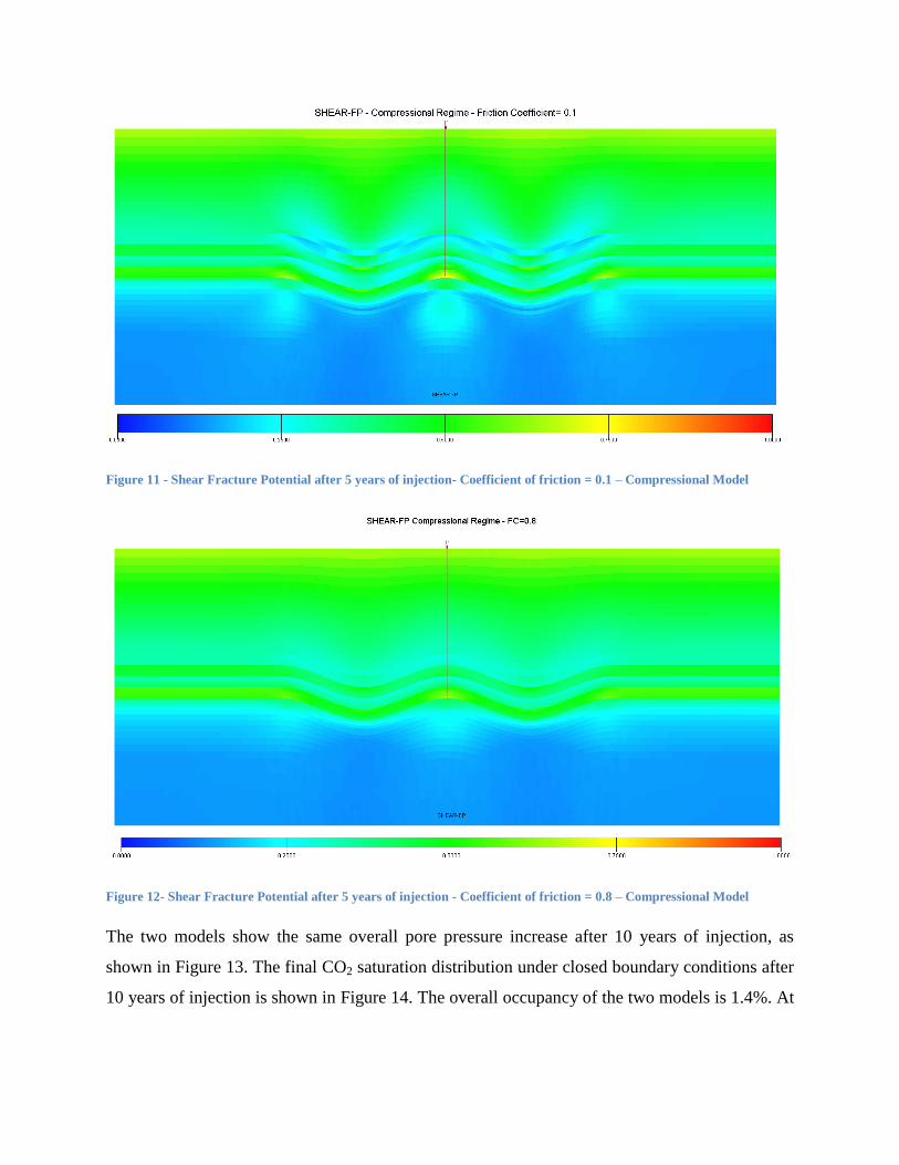
Figure 11 - Shear Fracture Potential after 5 years of injection- Coefficient of friction = 0.1 – Compressional Model
Figure 12- Shear Fracture Potential after 5 years of injection - Coefficient of friction = 0.8 – Compressional Model
The two models show the same overall pore pressure increase after 10 years of injection, as
shown in Figure 13. The final CO2 saturation distribution under closed boundary conditions after
10 years of injection is shown in Figure 14. The overall occupancy of the two models is 1.4%. At

this point hydraulic fractures are created in the vicinity of the well which can be considered good
for the overall performance of the model.
Figure 13- Pore pressure distribution in bar in the model after 10 years of injection
Figure 14 - Saturation of CO2 in the model after 10 years of injection
The two models, however, show different behaviors in terms of the shear fracture potential.
While the μ=0.8 is still at a safe state of stress, but close to shear failure at the well bore vicinity
after 10 years of injection, the μ=0.1 has already failed at this stage at the wellbore and the edges
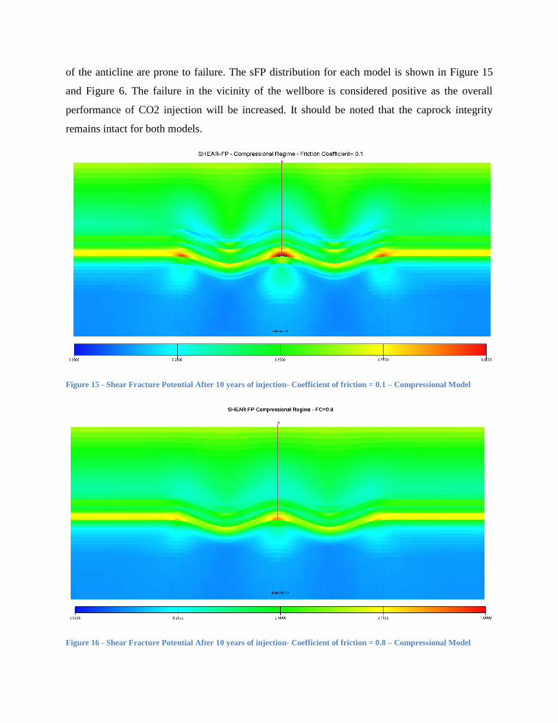
of the anticline are prone to failure. The sFP distribution for each model is shown in Figure 15
and Figure 6. The failure in the vicinity of the wellbore is considered positive as the overall
performance of CO2 injection will be increased. It should be noted that the caprock integrity
remains intact for both models.
Figure 15 - Shear Fracture Potential After 10 years of injection- Coefficient of friction = 0.1 – Compressional Model
Figure 16 - Shear Fracture Potential After 10 years of injection- Coefficient of friction = 0.8 – Compressional Model
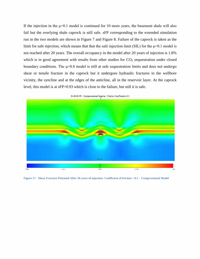
If the injection in the μ=0.1 model is continued for 10 more years, the basement shale will also
fail but the overlying shale caprock is still safe. sFP corresponding to the extended simulation
run in the two models are shown in Figure 7 and Figure 8. Failure of the caprock is taken as the
limit for safe injection, which means that that the safe injection limit (SIL) for the μ=0.1 model is
not reached after 20 years. The overall occupancy in the model after 20 years of injection is 1.8%
which is in good agreement with results from other studies for CO2 sequestration under closed
boundary conditions. The μ=0.8 model is still at safe sequestration limits and does not undergo
shear or tensile fracture in the caprock but it undergoes hydraulic fractures in the wellbore
vicinity, the syncline and at the edges of the anticline, all in the reservoir layer. At the caprock
level, this model is at sFP=0.93 which is close to the failure, but still it is safe.
Figure 17 - Shear Fracture Potential After 20 years of injection- Coefficient of friction = 0.1 – Compressional Model
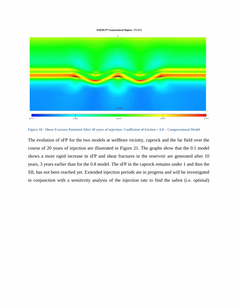
Figure 18 - Shear Fracture Potential After 20 years of injection- Coefficient of friction = 0.8 – Compressional Model
The evolution of sFP for the two models at wellbore vicinity, caprock and the far field over the
course of 20 years of injection are illustrated in Figure 21. The graphs show that the 0.1 model
shows a more rapid increase in sFP and shear fractures in the reservoir are generated after 10
years, 3 years earlier than for the 0.8 model. The sFP in the caprock remains under 1 and thus the
SIL has not been reached yet. Extended injection periods are in progress and will be investigated
in conjunction with a sensitivity analysis of the injection rate to find the safest (i.e. optimal)

scenario.
Figure 19 - sFP Evolution over Time at Wellbore - Compressional Regime
Figure 20 - sFP Evolution over Time at Far Field - Compressional Regime
0
0.2
0.4
0.6
0.8
1
0 5 10 15 20
She
ar F
ract
ure
Po
ten
tial
Injection Time, Years
sFP Evolution over Time at Wellbore Compressional Regime
μ=0.1
μ=0.8
0
0.2
0.4
0.6
0.8
1
0 5 10 15 20
She
ar F
ract
ure
Po
ten
tial
Injection Time, Years
sFP Evolution over Time at Caprock Compressional Regime
μ=0.1
μ=0.8

Figure 21 - sFP Evolution over Time at Far Field - Compressional Regime
1.2.4.2.2. Extensional Stress Regime
In the extensional regime, vertical stress is taken as the maximum principal stress and maximum
horizontal stress is considered the intermediate principal stress with minimum horizontal stress
being the minimum principal stress.
Figure 2 and Figure 3 show the initial shear fracture potential for the anticline with the
coefficient of friction of 0.1 and 0.8 between the layers under the Extensional regime
respectively.
0
0.2
0.4
0.6
0.8
1
0 5 10 15 20
She
ar F
ract
ure
Po
ten
tial
Injection Time, Years
sFP Evolution over Time at Far Field Compressional Regime
μ=0.1
μ=0.8
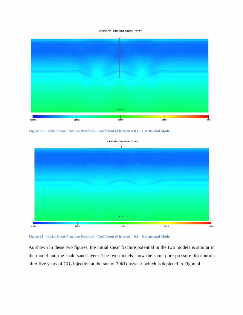
Figure 22 - Initial Shear Fracture Potential - Coefficient of friction = 0.1 – Extensional Model
Figure 23 - Initial Shear Fracture Potential - Coefficient of friction = 0.8 – Extensional Model
As shown in these two figures, the initial shear fracture potential in the two models is similar in
the model and the shale-sand layers. The two models show the same pore pressure distribution
after five years of CO2 injection at the rate of 20kTons/year, which is depicted in Figure 4.

Figure 24 - Pore pressure distribution in bar in the model after 5 years of injection
The increase in pore pressure will result in new states of stress and new sFP in the model models
as shown in Figure 5 and Figure 6. The two models undergo a decrease in shear fracture
potential, with sFP at the well bore vicinity decreasing from an initial value of 0.26 to 0.11 after
five years of injection for the μ=0.1 model and the μ=0.8 model goes from an initial sFP value of
0.24 to 0.11 after the same period of injection.
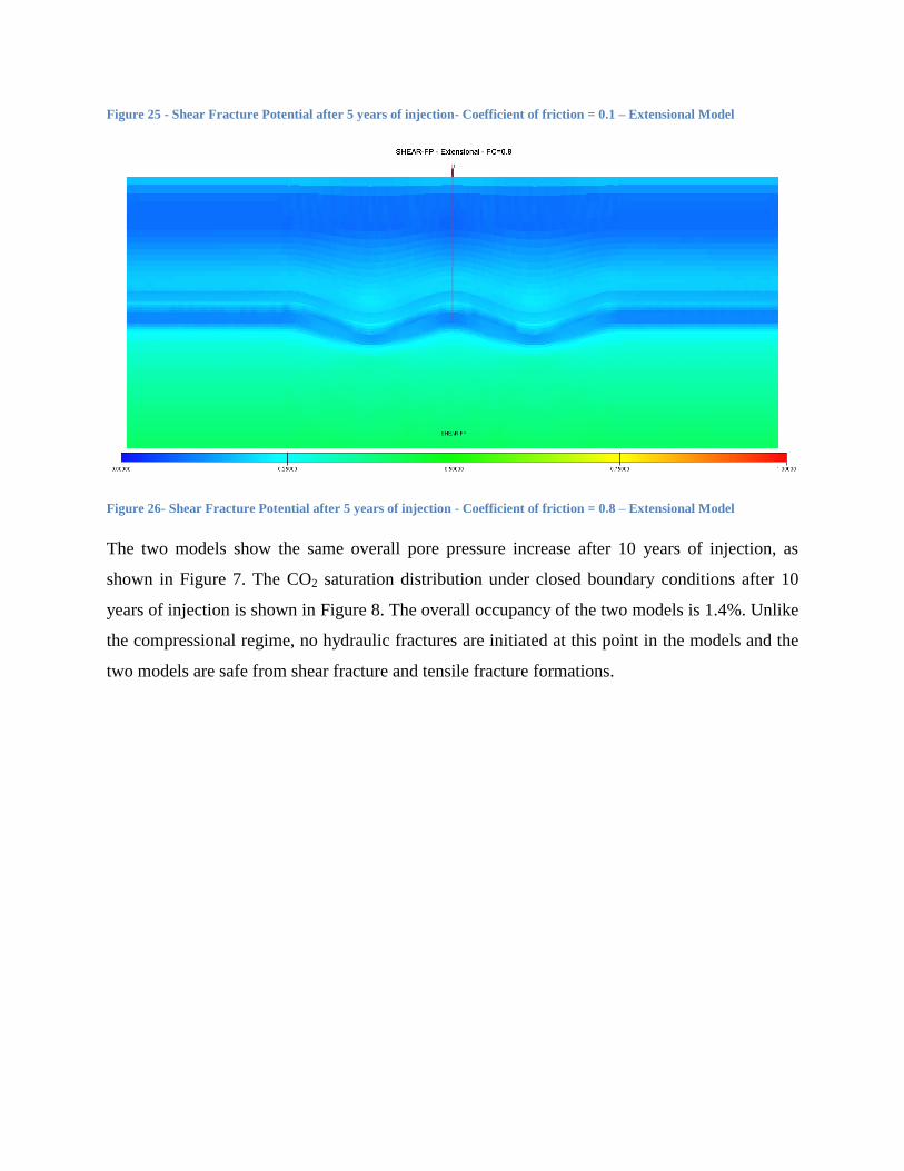
Figure 25 - Shear Fracture Potential after 5 years of injection- Coefficient of friction = 0.1 – Extensional Model
Figure 26- Shear Fracture Potential after 5 years of injection - Coefficient of friction = 0.8 – Extensional Model
The two models show the same overall pore pressure increase after 10 years of injection, as
shown in Figure 7. The CO2 saturation distribution under closed boundary conditions after 10
years of injection is shown in Figure 8. The overall occupancy of the two models is 1.4%. Unlike
the compressional regime, no hydraulic fractures are initiated at this point in the models and the
two models are safe from shear fracture and tensile fracture formations.
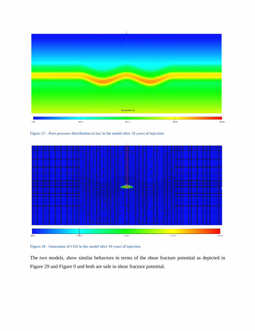
Figure 27 - Pore pressure distribution in bar in the model after 10 years of injection
Figure 28 - Saturation of CO2 in the model after 10 years of injection
The two models, show similar behaviors in terms of the shear fracture potential as depicted in
Figure 29 and Figure 0 and both are safe in shear fracture potential.
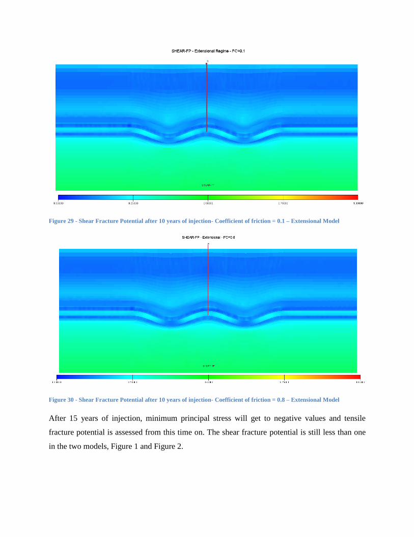
Figure 29 - Shear Fracture Potential after 10 years of injection- Coefficient of friction = 0.1 – Extensional Model
Figure 30 - Shear Fracture Potential after 10 years of injection- Coefficient of friction = 0.8 – Extensional Model
After 15 years of injection, minimum principal stress will get to negative values and tensile
fracture potential is assessed from this time on. The shear fracture potential is still less than one
in the two models, Figure 1 and Figure 2.
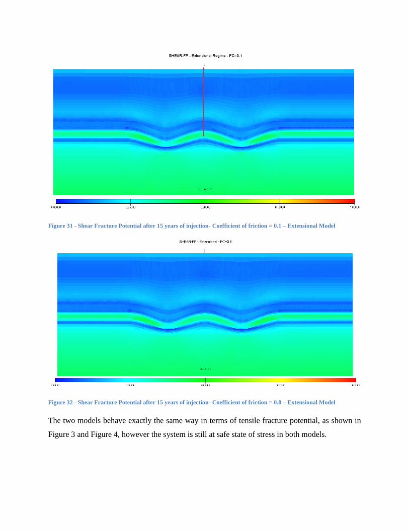
Figure 31 - Shear Fracture Potential after 15 years of injection- Coefficient of friction = 0.1 – Extensional Model
Figure 32 - Shear Fracture Potential after 15 years of injection- Coefficient of friction = 0.8 – Extensional Model
The two models behave exactly the same way in terms of tensile fracture potential, as shown in
Figure 3 and Figure 4, however the system is still at safe state of stress in both models.
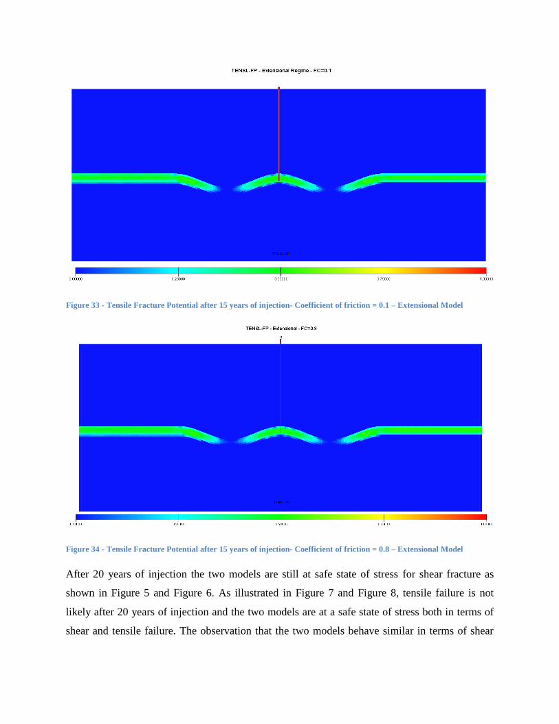
Figure 33 - Tensile Fracture Potential after 15 years of injection- Coefficient of friction = 0.1 – Extensional Model
Figure 34 - Tensile Fracture Potential after 15 years of injection- Coefficient of friction = 0.8 – Extensional Model
After 20 years of injection the two models are still at safe state of stress for shear fracture as
shown in Figure 5 and Figure 6. As illustrated in Figure 7 and Figure 8, tensile failure is not
likely after 20 years of injection and the two models are at a safe state of stress both in terms of
shear and tensile failure. The observation that the two models behave similar in terms of shear

fracture and tensile fracture denotes that the coefficient of friction does not play an important
role under the extensional regime.
Figure 35 - Shear Fracture Potential after 20 years of injection- Coefficient of friction = 0.1 – Extensional Model
Figure 36 - Shear Fracture Potential after 20 years of injection- Coefficient of friction = 0.8 – Extensional Model
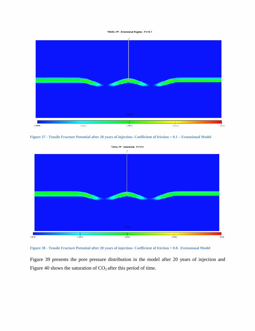
Figure 37 - Tensile Fracture Potential after 20 years of injection- Coefficient of friction = 0.1 – Extensional Model
Figure 38 - Tensile Fracture Potential after 20 years of injection- Coefficient of friction = 0.8– Extensional Model
Figure 39 presents the pore pressure distribution in the model after 20 years of injection and
Figure 40 shows the saturation of CO2 after this period of time.
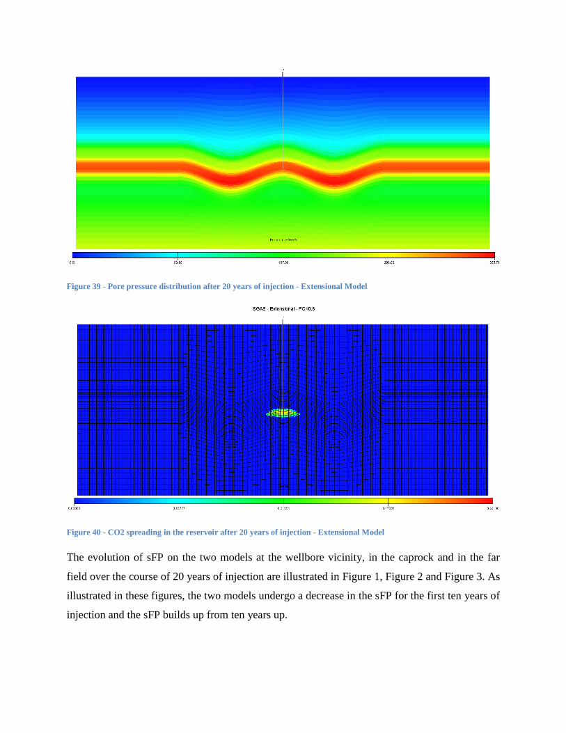
Figure 39 - Pore pressure distribution after 20 years of injection - Extensional Model
Figure 40 - CO2 spreading in the reservoir after 20 years of injection - Extensional Model
The evolution of sFP on the two models at the wellbore vicinity, in the caprock and in the far
field over the course of 20 years of injection are illustrated in Figure 1, Figure 2 and Figure 3. As
illustrated in these figures, the two models undergo a decrease in the sFP for the first ten years of
injection and the sFP builds up from ten years up.
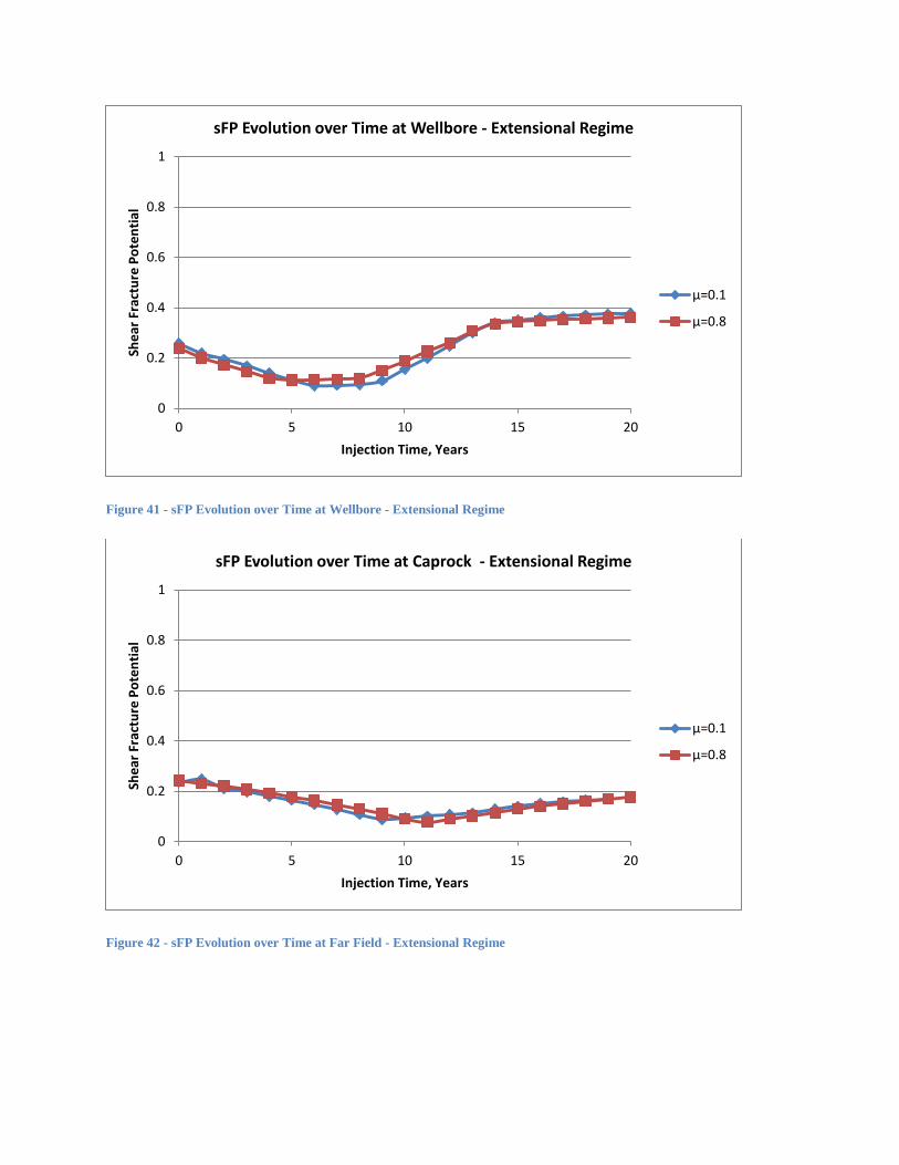
Figure 41 - sFP Evolution over Time at Wellbore - Extensional Regime
Figure 42 - sFP Evolution over Time at Far Field - Extensional Regime
0
0.2
0.4
0.6
0.8
1
0 5 10 15 20
She
ar F
ract
ure
Po
ten
tial
Injection Time, Years
sFP Evolution over Time at Wellbore - Extensional Regime
μ=0.1
μ=0.8
0
0.2
0.4
0.6
0.8
1
0 5 10 15 20
She
ar F
ract
ure
Po
ten
tial
Injection Time, Years
sFP Evolution over Time at Caprock - Extensional Regime
μ=0.1
μ=0.8
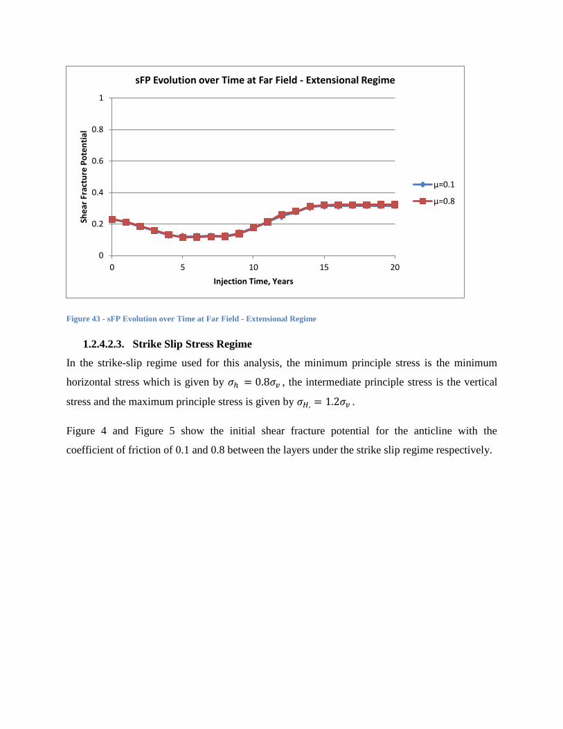
Figure 43 - sFP Evolution over Time at Far Field - Extensional Regime
1.2.4.2.3. Strike Slip Stress Regime
In the strike-slip regime used for this analysis, the minimum principle stress is the minimum
horizontal stress which is given by , the intermediate principle stress is the vertical
stress and the maximum principle stress is given by .
Figure 4 and Figure 5 show the initial shear fracture potential for the anticline with the
coefficient of friction of 0.1 and 0.8 between the layers under the strike slip regime respectively.
0
0.2
0.4
0.6
0.8
1
0 5 10 15 20
She
ar F
ract
ure
Po
ten
tial
Injection Time, Years
sFP Evolution over Time at Far Field - Extensional Regime
μ=0.1
μ=0.8

Figure 44 - Initial Shear Fracture Potential - Coefficient of friction = 0.1 – Strike Slip Model
Figure 45 - Initial Shear Fracture Potential - Coefficient of friction = 0.8 – Strike Slip Model
As shown in these two figures, the initial shear fracture potential in the two models is similar in
the model and the shale-sand layers. The two models show the same pore pressure distribution
after five years of CO2 injection at the rate of 20kTons/year, which is depicted in Figure 6.
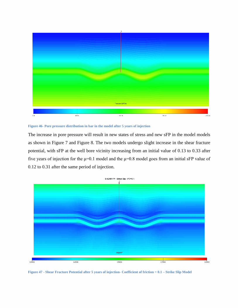
Figure 46- Pore pressure distribution in bar in the model after 5 years of injection
The increase in pore pressure will result in new states of stress and new sFP in the model models
as shown in Figure 7 and Figure 8. The two models undergo slight increase in the shear fracture
potential, with sFP at the well bore vicinity increasing from an initial value of 0.13 to 0.33 after
five years of injection for the μ=0.1 model and the μ=0.8 model goes from an initial sFP value of
0.12 to 0.31 after the same period of injection.
Figure 47 - Shear Fracture Potential after 5 years of injection- Coefficient of friction = 0.1 – Strike Slip Model
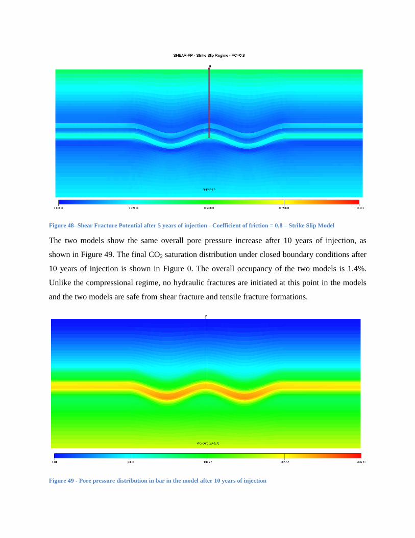
Figure 48- Shear Fracture Potential after 5 years of injection - Coefficient of friction = 0.8 – Strike Slip Model
The two models show the same overall pore pressure increase after 10 years of injection, as
shown in Figure 49. The final CO2 saturation distribution under closed boundary conditions after
10 years of injection is shown in Figure 0. The overall occupancy of the two models is 1.4%.
Unlike the compressional regime, no hydraulic fractures are initiated at this point in the models
and the two models are safe from shear fracture and tensile fracture formations.
Figure 49 - Pore pressure distribution in bar in the model after 10 years of injection
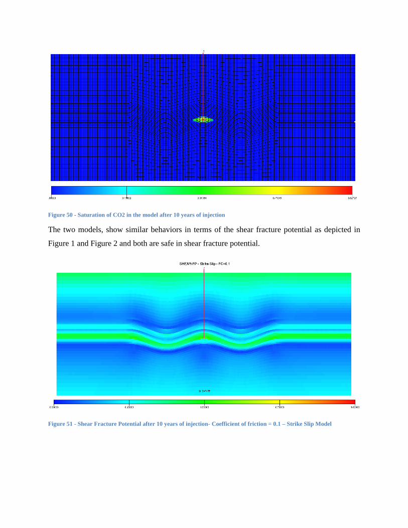
Figure 50 - Saturation of CO2 in the model after 10 years of injection
The two models, show similar behaviors in terms of the shear fracture potential as depicted in
Figure 1 and Figure 2 and both are safe in shear fracture potential.
Figure 51 - Shear Fracture Potential after 10 years of injection- Coefficient of friction = 0.1 – Strike Slip Model
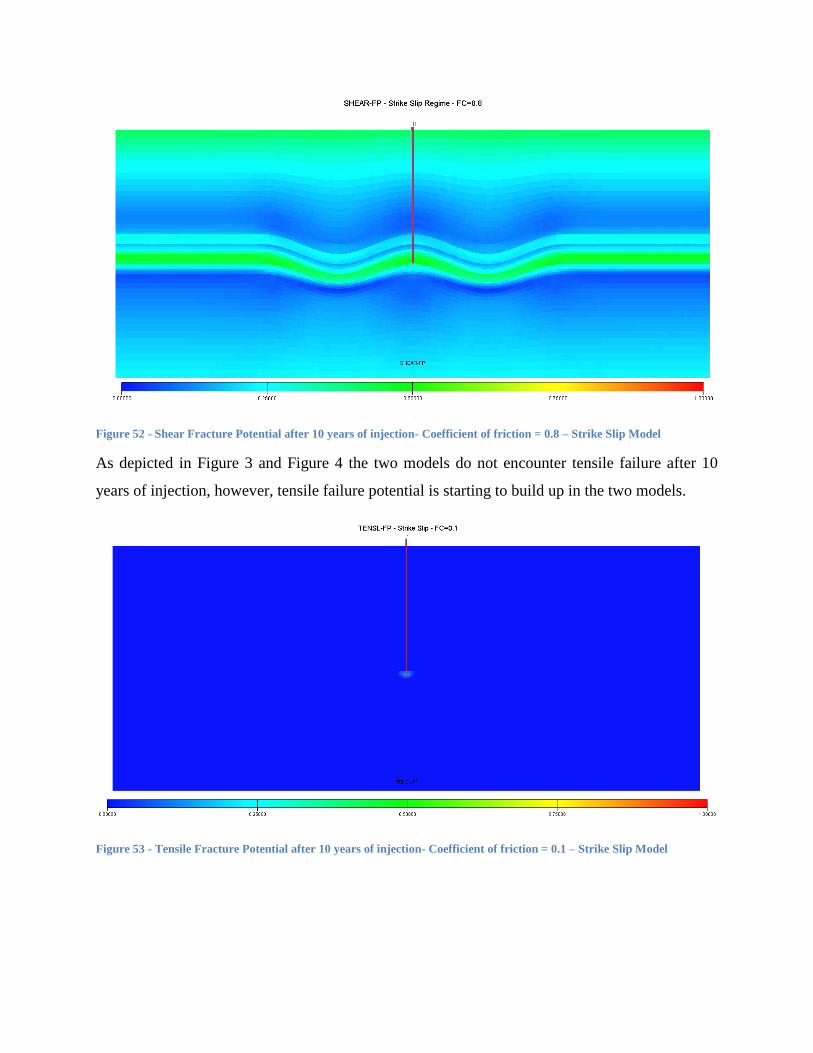
Figure 52 - Shear Fracture Potential after 10 years of injection- Coefficient of friction = 0.8 – Strike Slip Model
As depicted in Figure 3 and Figure 4 the two models do not encounter tensile failure after 10
years of injection, however, tensile failure potential is starting to build up in the two models.
Figure 53 - Tensile Fracture Potential after 10 years of injection- Coefficient of friction = 0.1 – Strike Slip Model

Figure 54 - Tensile Fracture Potential after 10 years of injection- Coefficient of friction = 0.8 – Strike Slip Model
After 20 years of injection, Figure 5 and Figure 6, the two models are still at stable state from the
shear failure point of view but they experience tensile fractures in the reservoir layer around the
wellbore as illustrated in Figure 7 and Figure 8.
Figure 55 - Shear Fracture Potential after 20 years of injection- Coefficient of friction = 0.1 – Strike Slip Model
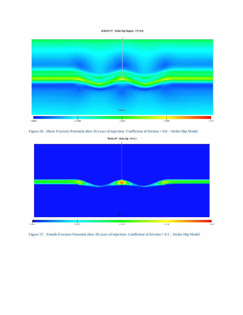
Figure 56 - Shear Fracture Potential after 20 years of injection- Coefficient of friction = 0.8 – Strike Slip Model
Figure 57 - Tensile Fracture Potential after 20 years of injection- Coefficient of friction = 0.1 – Strike Slip Model
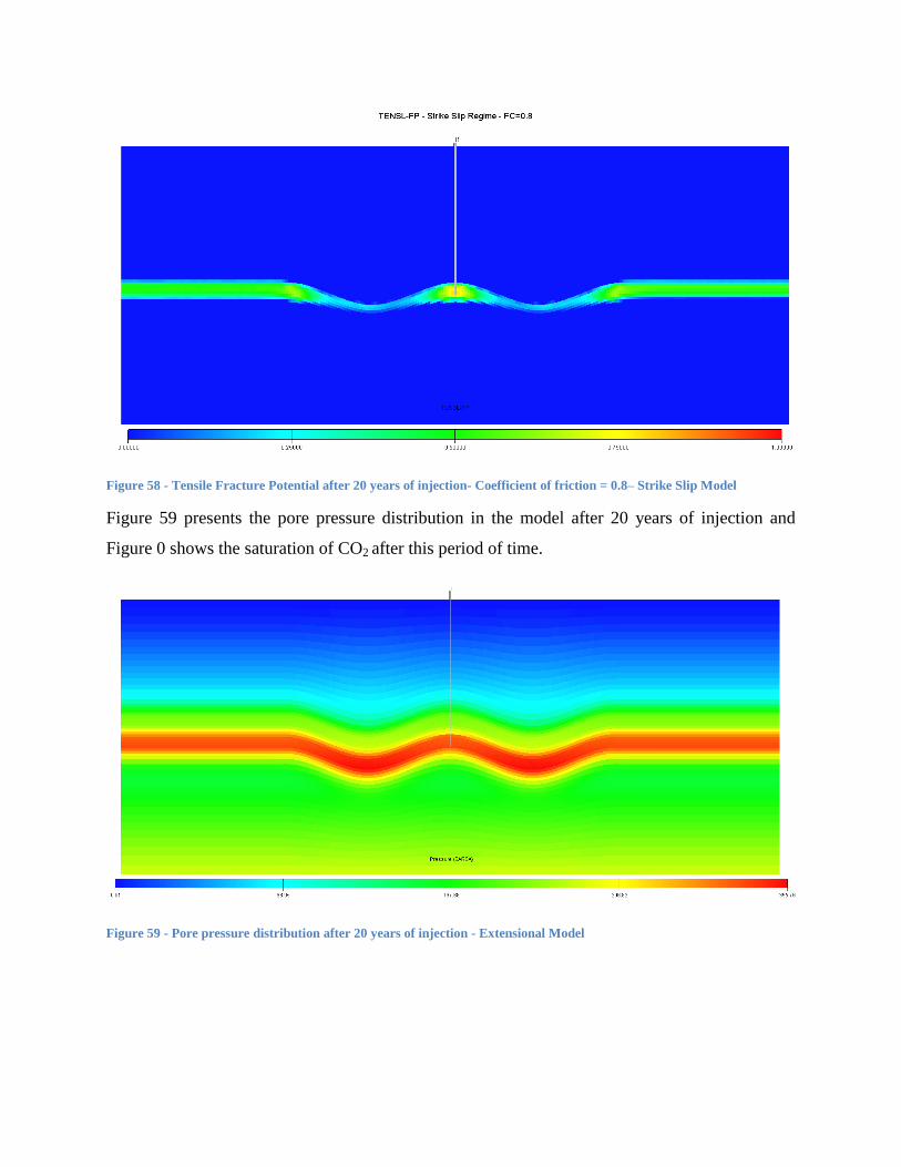
Figure 58 - Tensile Fracture Potential after 20 years of injection- Coefficient of friction = 0.8– Strike Slip Model
Figure 59 presents the pore pressure distribution in the model after 20 years of injection and
Figure 0 shows the saturation of CO2 after this period of time.
Figure 59 - Pore pressure distribution after 20 years of injection - Extensional Model

Figure 60 - CO2 spreading in the reservoir after 20 years of injection - Extensional Model
The evolution of sFP on the two models at wellbore vicinity, caprock and the far field over the
course of 20 years of injection are illustrated in Figure 3. The sFP trend show a sensitivity to the
coefficient of friction, with the 0.1 model observing higher sFP values near the injection
location. For the cap rock and the far-field the sFP values are almost identical for both
coefficients of friction.
Tensile FP is steadily increased over the injection period and even reaches values of 1 near the
injection location in the 0.1 model, however tFP does not reach the caprock which remains stable
wih low tFP values (0-0.1).

Figure 61 - sFP Evolution over Time at Wellbore - Strike Slip Regime
Figure 62 - sFP Evolution over Time at Caprock- Strike Slip Regime
0
0.2
0.4
0.6
0.8
1
0 5 10 15 20
She
ar F
ract
ure
Po
ten
tial
Injection Time, Years
sFP Evolution over Time at Wellbore Strike Slip Regime
μ=0.1
μ=0.8
0
0.2
0.4
0.6
0.8
1
0 5 10 15 20
She
ar F
ract
ure
Po
ten
tial
Injection Time, Years
sFP Evolution over Time at Caprock Strike Slip Regime
μ=0.1
μ=0.8

Figure 63- sFP Evolution over Time at Far Field - Strike Slip Regime
1.2.5. Discussion
Estimating and simulating the maximum sustainable pore pressure change, ΔPc, before optimally
oriented fractures are reactivated represents a key component of geomechanical risk analyses for
CO2 injection applications (e.g. Streit and Hillis, 2004; Rutqvist et al., 2007; Cappa and Rutvist,
2011; Paradeis et al., 2012). These analyses become especially relevant when structural trap
systems such as anticlines are considered for CO2 sequestration. Anticline structures have a
heterogeneous state of stress whereby the horizontal stresses change rapidly at the top of the
crest to the bottom of the crest (Paradeis et al., 2012).
As shown by equations 3-5 simplified analytical solutions based on the principle of pore pressure
– stress coupling (Altmann et al., 2010) can be used to calculate the maximum sustainable pore
pressure, Pc, prior to CO2 injection. The results presented show that Pc is strongly dependent on
the stress regime and the relative location with respect to the injection location. Based on these
calculations different stress regimes result in significant differences between horizontally layered
sedimentary basins and anticlines. In this respect the case of horizontally layered basins in an
extensional stress regime merits special consideration. If such basins are tectonically relieved the
0
0.2
0.4
0.6
0.8
1
0 5 10 15 20
She
ar F
ract
ure
Po
ten
tial
Injection Time, Years
sFP Evolution over Time at Far Field Strike Slip Regime
μ=0.1
μ=0.8
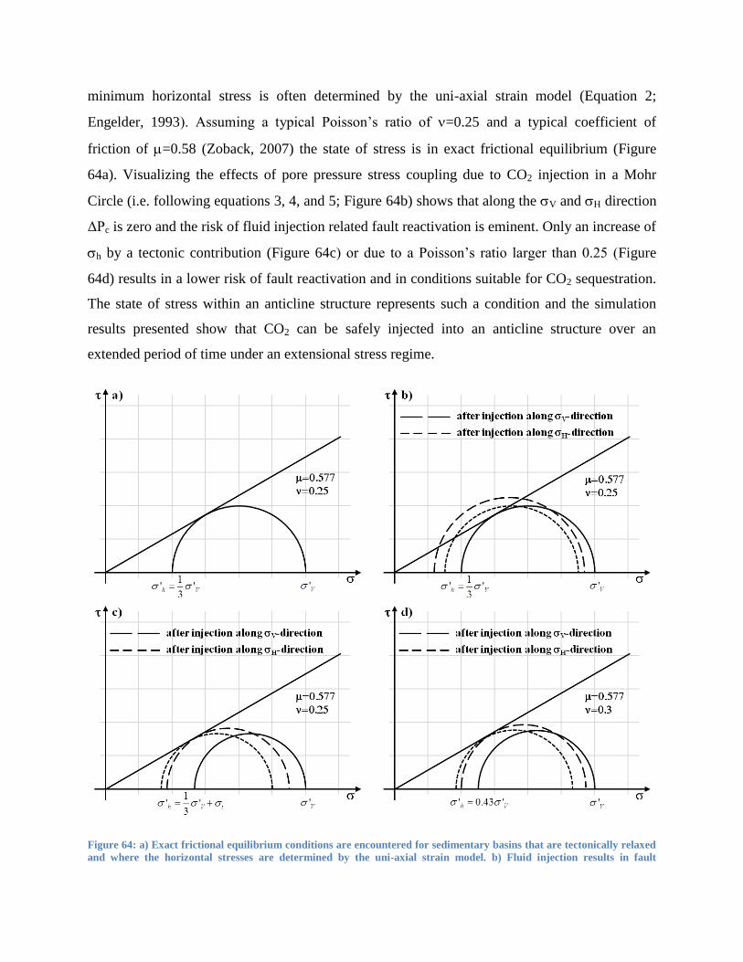
minimum horizontal stress is often determined by the uni-axial strain model (Equation 2;
Engelder, 1993). Assuming a typical Poisson’s ratio of =0.25 and a typical coefficient of
friction of =0.58 (Zoback, 2007) the state of stress is in exact frictional equilibrium (Figure
64a). Visualizing the effects of pore pressure stress coupling due to CO2 injection in a Mohr
Circle (i.e. following equations 3, 4, and 5; Figure 64b) shows that along the V and direction
ΔPc is zero and the risk of fluid injection related fault reactivation is eminent. Only an increase of
h by a tectonic contribution (Figure 64c) or due to a Poisson’s ratio larger than 0.25 (Figure
64d) results in a lower risk of fault reactivation and in conditions suitable for CO2 sequestration.
The state of stress within an anticline structure represents such a condition and the simulation
results presented show that CO2 can be safely injected into an anticline structure over an
extended period of time under an extensional stress regime.
Figure 64: a) Exact frictional equilibrium conditions are encountered for sedimentary basins that are tectonically relaxed
and where the horizontal stresses are determined by the uni-axial strain model. b) Fluid injection results in fault
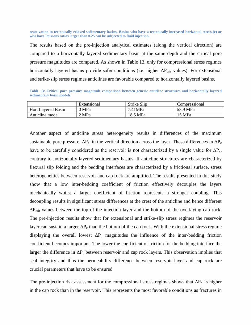
reactivation in tectonically relaxed sedimentary basins. Basins who have a tectonically increased horizontal stress (c) or
who have Poissons ratios larger than 0.25 can be subjected to fluid injection.
The results based on the pre-injection analytical estimates (along the vertical direction) are
compared to a horizontally layered sedimentary basin at the same depth and the critical pore
pressure magnitudes are compared. As shown in Table 13, only for compressional stress regimes
horizontally layered basins provide safer conditions (i.e. higher ΔPcrit values). For extensional
and strike-slip stress regimes anticlines are favorable compared to horizontally layered basins.
Table 13: Critical pore pressure magnitude comparison between generic anticline structures and horizontally layered
sedimentary basin models.
Extensional Strike Slip Compressional
Hor. Layered Basin 0 MPa 7.41MPa 58.9 MPa
Anticline model 2 MPa 18.5 MPa 15 MPa
Another aspect of anticline stress heterogeneity results in differences of the maximum
sustainable pore pressure, ΔPc, in the vertical direction across the layer. These differences in ΔPc
have to be carefully considered as the reservoir is not characterized by a single value for ΔPc,
contrary to horizontally layered sedimentary basins. If anticline structures are characterized by
flexural slip folding and the bedding interfaces are characterized by a frictional surface, stress
heterogeneities between reservoir and cap rock are amplified. The results presented in this study
show that a low inter-bedding coefficient of friction effectively decouples the layers
mechanically whilst a larger coefficient of friction represents a stronger coupling. This
decoupling results in significant stress differences at the crest of the anticline and hence different
ΔPcrit values between the top of the injection layer and the bottom of the overlaying cap rock.
The pre-injection results show that for extensional and strike-slip stress regimes the reservoir
layer can sustain a larger ΔPc than the bottom of the cap rock. With the extensional stress regime
displaying the overall lowest ΔPc magnitudes the influence of the inter-bedding friction
coefficient becomes important. The lower the coefficient of friction for the bedding interface the
larger the difference in ΔPc between reservoir and cap rock layers. This observation implies that
seal integrity and thus the permeability difference between reservoir layer and cap rock are
crucial parameters that have to be ensured.
The pre-injection risk assessment for the compressional stress regimes shows that ΔPc is higher
in the cap rock than in the reservoir. This represents the most favorable conditions as fractures in

the reservoir rock can be reactivated, thus increasing infectivity, whilst the cap rock remains
stable.
The results based on the simplified analytical derivations (i.e. using long-term limits) show that
they are useful to obtain a quick 1st order estimate on Pc prior to injection to estimate fault
reactivation risk. Furthermore, for the specific location along the crest of the anticline the
influence of specific geological parameters such as the inter-bedding friction coefficient can be
demonstrated. It is clear that the true nature of pore pressure - stress coupling is much more
complex (Altmann et al., 2010). In order to include the spatial and temporal relationships
coupled numerical analyses involving all physical processes are necessary.
It should be noted that due to the licensing (ECLIPSE) problems at Missouri S&T in the final 2
project quarters of the project only fracture generation results have been calculated and analyzed
for the coupled simulations and thus cannot be compared to the analytical estimates based on
fracture reactivation. The results for fracture reactivation would show an overall increased risk
for failure and the applied parameter of fracture potential.
The results show that the stress regime has a significant influence on the geomechanical risk
assessment. As expected from pore pressure stress coupling theory, the compressional stress
regime results in increasing differential stresses and the risk for shear failure is evident. The
results also show that pore pressure-stress coupling is dependent on the direction and distance to
the injection point. The results for the compressional regime show that FP increases at a higher
rate in the lateral direction from than injection well than in the vertical direction. On the other
hand the extensional stress regime exhibits the safest conditions and within the 20 year injection
period modeled neither tensile nor shear failure is observed.
Furthermore, the more compressional the stress regime, the larger is the difference between the
models with a different inter-bedding plane coefficient of friction. The compressional stress
regime exhibits a much lower ΔPc magnitudes for low friction coefficients. This result is
confirmed as shown by the pre-injection estimate (Figure 5a).
The results presented over a 20 injection period result only show elevated geomechanical risks
for the compressional stress regime. However, with shear fracture potential steadily increasing in
the strike slip regime and tensile fracture potential increasing in the extensional regime, a longer
injection period is necessary. Model runs for a 50 year injection period and longer are
recommended to analyze for similar case studies. It is important to note that whilst the anticline
structures investigated in this study represent generic structures the results presented have shown
that stress heterogeneities due to the geometry of a geological structures have an important
impact on the resulting geomechanical risks and should not be neglected. Also, whilst the
absolute magnitudes of the results of this study are not representative of a “real” geologic
structure, the relative importance of geometry, stress regime and inter-bedding friction has been
shown and the procedure can be readily applied to a real case study.
1.2.6. Conclusions
The analytical pre-injection estimates together with the coupled simulations have shown and
confirmed that the in-situ stress regime is a crucial, if not the most important, factor determining
geomechanical risks, for fluid injection applications such as CO2 sequestration. It is therefore
strongly recommended that every case study is based on in-situ stress measurements for a
thorough calibration of numerical models used to analyze geomechanical risks.
The coupled simulations for the generic anticline structures have shown that the extensional
stress regime represents the overall safest scenario, however is considered the most unlikely as
anticlines are compressional structures. The compressional stress regime shows reservoir failure
after 20 years of CO2 injection. Whilst this is considered favorable as failure in the injection
layer increases overall injectivity, the caprock is also very close to failure and a longer injection
periods would thus require adjustment of the injection parameters. It should be noted again that
the coupled modeling result are for fracture generation and fracture reactivation would occur
much earlier, enhancing the geomechanical risks, and resulting in shorter safe injection times.
The generic anticline geometries investigated in this study have shown that in addition to the in-
situ state of stress the stress heterogeneities associated to the geometry of such structures result
in significant differences with respect to sustainable pore pressure magnitudes. For extension and
strike slip stress regimes anticline structures should be favored over horizontally layered basin as
they feature higher ΔPc magnitudes. If sedimentary basins are tectonically relaxed and their state
of stress is characterized by the uni-axial strain model the basin is in exact frictional equilibrium
and fluids should not be injected.
Another important observation from the generic models is the influence of geological parameters
such as the inter-bedding friction coefficient. Whilst the influence of this parameter is not
important for horizontally layered structures, the geometry of anticline structures results in stress
heterogeneities and the coefficient of friction on bedding planes determines the mechanical
coupling between different layers. The results have shown that low friction coefficients
effectively decouple layers resulting in lower ΔPc magnitudes, especially for the compressional
stress regime.
2. Wellbore Scale Model
2.1.Model Initialization
2.1.1. Introduction
Many applications of wellbore stability analysis, wellbore design, cementing as well as hydraulic
fracturing processes rely on an accurate representation of the state of stress in the near-wellbore
region. The analytical solution of the borehole stresses for a linear elastic material is given by the
well known solution derived by Ernst Gustav Kirsch in 1898. Bradley [1979] and Zhang et al.
[2006] further derived the effective wellbore stresses at the borehole wall for an inclined
borehole including pore pressure and mud pressure. However, the analytical solution has
limitations handling complex formation geometry, material heterogeneities and different
rheological models. As computers and commercial numerical software applications have become
readily available as a standard engineering tool a variety of borehole stress studies utilize 2D and
3D finite element analysis for solving geomechanical problems associated with borehole failure
[Cheng and Dusseault, 1993; Zervos et al., 1998; Gentzis et al., 2009]. It should be noted that
numerical modeling methods introduce errors by nature, as they represent an approximation
approach [Zienkiewiscz et al. 2006], and often utilize assumptions and simplifications of the
physical problem. Thus, a common problem of numerical studies is the validation and calibration
to analytical solutions and field data. Since this standard modeling procedure is sometimes not
available, care has to be taken with numerical codes to provide an accurate solution before the
results can be relied on for interpretation.
For wellbore stress analyses the accuracy of numerical modeling results becomes crucial
especially at the wellbore wall where the state of stress changes rapidly and it is therefore
recommended to ensure a high quality mesh to obtain accurate results. The optimization of the
mesh quality may not be done in every study [Rutqvist et al., 1989; Zahn et al., 2010], and to
date only few studies have shown that mesh quality has a significant influence on numerical
modeling results in geomechanical applications [Nipp et al., 1987; Grabinsky et al., 1995; Turon
et al., 2007]. Grabinsky et al. [1995] studied the impact of different element types providing
good quality discretizations for rock excavation scenarios. Turon et al. [2007] showed that
results are sensitive to the element size when handling pore cohesive elements in the wellbore
fracture zone, and a mesh size as small as 0.5mm in length is necessary to obtain converging
solutions. Nipp and McNulty [1987] demonstrated how boundary conditions and element size
can affect the accuracy of solutions involving creep around a single borehole in an infinite
medium. In summary, these studies support the inference that the discretization parameters of
element size, element type, model size and boundary conditions are crucial regarding the
accuracy of numerical results.
In this paper we present a general guideline to generate an optimized mesh for wellbore stress
analysis of non-inclined wellbores and show how the boundary conditions and discretization
parameters of the model can affect the accuracy of the calculated stresses around the wellbore.
We use a parametric study on model size, element size, element type and boundary condition
application and compare and validate the numerical results to the analytical solution. In the
context of a safe mud weight window prediction study for three different stress regimes, we
show how errors from non-optimized meshes can lead to a significant under- or over-estimation
of the safe mud weight window.
2.1.2. Theoretical Background
a) Analytical Solution for Wellbore Stresses
Before drilling, the state of stress of the rock in the subsurface is in equilibrium and can be
represented by the three in-situ principal stresses σ1, σ2, and σ3, which for an Andersonian state
of stress, are the vertical stress and two far field horizontal stresses [Pollard and Fletcher, 2005].
During drilling, the borehole rock is removed and the acting loads are to be compensated by the
adjacent rock around the wellbore. After redistribution of the stresses, local stress concentrations
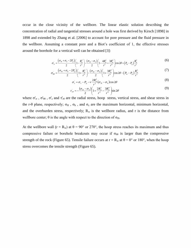
occur in the close vicinity of the wellbore. The linear elastic solution describing the
concentration of radial and tangential stresses around a hole was first derived by Kirsch [1898] in
1898 and extended by Zhang et al. [2006] to account for pore pressure and the fluid pressure in
the wellbore. Assuming a constant pore and a Biot’s coefficient of 1, the effective stresses
around the borehole for a vertical well can be obtained [3]:
2 2 4 2'
2 2 4 2
2 4 31 1 cos 2
2 2
H h p H hw w w wrr m p
P R R R RP P
r r r r
(6)
2 4 2'
2 4 2
2 31 1 cos 2
2 2
H h p H hw w wm p
P R R RP P
r r r
(7)
2cos
22
2'
hHw
pvzr
RP (8)
2sin
321
2 4
4
2
2'
r
R
r
R wwhHr
(9)
where σ'rr , σ'θθ , σ'z and τ'rθ are the radial stress, hoop stress, vertical stress, and shear stress in
the r-θ plane, respectively; σH , σh , and σz are the maximum horizontal, minimum horizontal,
and the overburden stress, respectively; Rw is the wellbore radius, and r is the distance from
wellbore center; θ is the angle with respect to the direction of σH.
At the wellbore wall (r = Rw) at θ = 90° or 270°, the hoop stress reaches its maximum and thus
compressive failure or borehole breakouts may occur if σθθ is larger than the compressive
strength of the rock (Figure 65). Tensile failure occurs at r = Rw at θ = 0° or 180°, when the hoop
stress overcomes the tensile strength (Figure 65).
Fig. 65. A vertical wellbore showing the state of stress and potential failure types around the borehole: σrr is the radial
stress, σθθ is the hoop stress, Pp is the pore fluid pressure in the rock formation and Pm is the drilling fluid pressure.
Vertical stress σz is along the borehole axis and is not shown in the figure.
b) Failure Criteria
The criterion for tensile failure at the borehole wall is given when the minimum effective
principal stress '3 is less than the formation tensile strength T0:
0
'
3 T (10)
In order to predict compressive rock failure, different failure criteria are commonly applied
[McLean and Addis, 1990]. These criteria can be categorized into criteria, where failure is only
dependent on the differential stress σ1 – σ3, such as the Mohr-Coulomb criterion, or into criteria
accounting for a strength dependence of the intermediate principal stress (σ2), such as the
Drucker-Prager or the modified Lade criterion [Zhang et al., 2010].
Studies have shown that the choice of the applied failure criterion has a significant influence on
the prediction of the safe minimum mud weight [Ewy, 1999; Nawrocki, 2010; Tran et al., 2010].
It should be noted that for the subsequent analysis the evaluation of an appropriate failure
criterion for wellbore stability analysis is beyond the scope of this paper and that the errors
introduced by non-optimized meshes result in errors of the numerically determined hoop and
radial stresses. For the linear elastic, isotropic analysis applied in this study theses numerical
errors are independent from the application of the relevant failure criterion. Thus, for simplicity
we chose the Mohr-Coulomb failure criterion as the example of the most conservative criterion
[Zhang et al., 2010] for predicting the minimum mud weight to ensure wellbore stability. The
Mohr-Coulomb [Coulomb, 1776] failure criterion represents the linear envelope that can be
expressed by the normal stress and shear stress on a failure plane:
tan0 nC (11)
where τ is the shear stress, σn is the normal stress, C0 is the cohesion and φ is the internal friction
angle of the rock. When the Mohr circle, defined by σ1 and σ3, intersects with the failure
envelope, shear failure will occur, and the failure criterion can be expressed in terms of the
relation of σ1 and σ3 at failure:
301
sin1
sin1
sin1
cos2
C (12)
c) Safe Mud Weight prediction
The safe mud weight window for drilling is defined by the collapse pressure as the lower limit to
prevent the onset of breakouts and the breakdown pressure as the upper limit to prevent the onset
of tensile failure. In permeable formations mud pressure is required to be higher than the pore
fluid pressure to prevent kicks to occur. If the required mud pressure is higher than the collapse
pressure, the mud pressure is chosen as the lower limit of the safe mud weight window. Based on
the Mohr-Coulomb failure criterion, the collapse pressure can be solved for by utilizing Eq. (13)
and the fact that the two Mohr circles have the same mean stress:
sin1
sin11
sin1
cos2
22
0
''
3
13
''
Crr
rr
(13)
Pm, collapse can be solved for by the fact that σ3 equals to σ'rr added by Pm,collapse (Eq. (14)) or
σ1 equals σ'θθ subtracted by Pm,collapse (Eq. (15)):
1
''
3, orP rrcollapsem (14)
The breakdown pressure is calculated by:
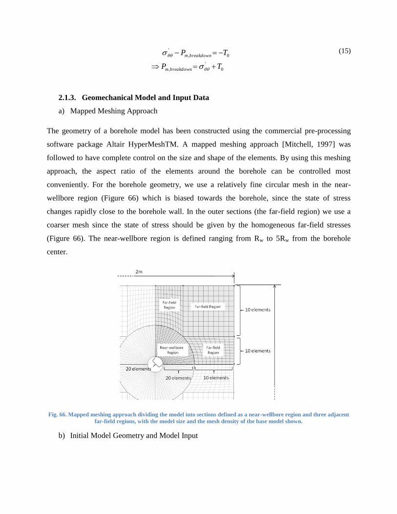
0
'
,
0,
'
TP
TP
breakdownm
breakdownm
(15)
2.1.3. Geomechanical Model and Input Data
a) Mapped Meshing Approach
The geometry of a borehole model has been constructed using the commercial pre-processing
software package Altair HyperMeshTM. A mapped meshing approach [Mitchell, 1997] was
followed to have complete control on the size and shape of the elements. By using this meshing
approach, the aspect ratio of the elements around the borehole can be controlled most
conveniently. For the borehole geometry, we use a relatively fine circular mesh in the near-
wellbore region (Figure 66) which is biased towards the borehole, since the state of stress
changes rapidly close to the borehole wall. In the outer sections (the far-field region) we use a
coarser mesh since the state of stress should be given by the homogeneous far-field stresses
(Figure 66). The near-wellbore region is defined ranging from Rw to 5Rw from the borehole
center.
Fig. 66. Mapped meshing approach dividing the model into sections defined as a near-wellbore region and three adjacent
far-field regions, with the model size and the mesh density of the base model shown.
b) Initial Model Geometry and Model Input
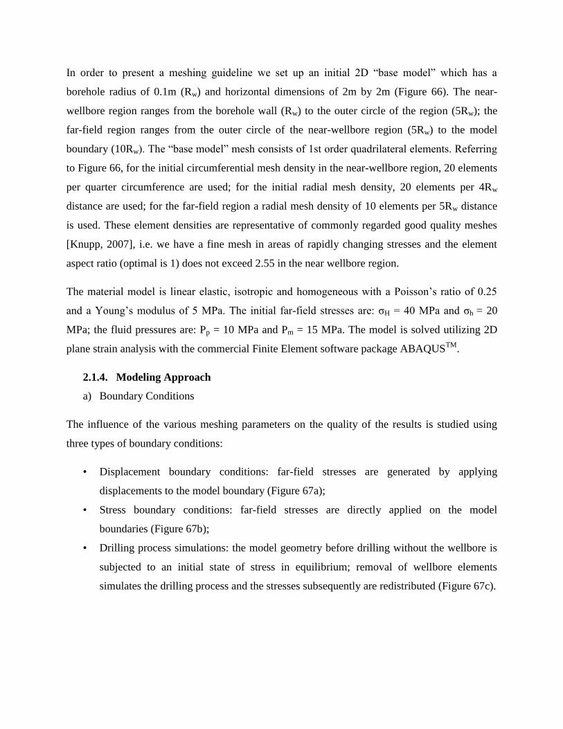
In order to present a meshing guideline we set up an initial 2D “base model” which has a
borehole radius of 0.1m (Rw) and horizontal dimensions of 2m by 2m (Figure 66). The near-
wellbore region ranges from the borehole wall (Rw) to the outer circle of the region (5Rw); the
far-field region ranges from the outer circle of the near-wellbore region (5Rw) to the model
boundary (10Rw). The “base model” mesh consists of 1st order quadrilateral elements. Referring
to Figure 66, for the initial circumferential mesh density in the near-wellbore region, 20 elements
per quarter circumference are used; for the initial radial mesh density, 20 elements per 4Rw
distance are used; for the far-field region a radial mesh density of 10 elements per 5Rw distance
is used. These element densities are representative of commonly regarded good quality meshes
[Knupp, 2007], i.e. we have a fine mesh in areas of rapidly changing stresses and the element
aspect ratio (optimal is 1) does not exceed 2.55 in the near wellbore region.
The material model is linear elastic, isotropic and homogeneous with a Poisson’s ratio of 0.25
and a Young’s modulus of 5 MPa. The initial far-field stresses are: σH = 40 MPa and σh = 20
MPa; the fluid pressures are: Pp = 10 MPa and Pm = 15 MPa. The model is solved utilizing 2D
plane strain analysis with the commercial Finite Element software package ABAQUSTM
.
2.1.4. Modeling Approach
a) Boundary Conditions
The influence of the various meshing parameters on the quality of the results is studied using
three types of boundary conditions:
• Displacement boundary conditions: far-field stresses are generated by applying
displacements to the model boundary (Figure 67a);
• Stress boundary conditions: far-field stresses are directly applied on the model
boundaries (Figure 67b);
• Drilling process simulations: the model geometry before drilling without the wellbore is
subjected to an initial state of stress in equilibrium; removal of wellbore elements
simulates the drilling process and the stresses subsequently are redistributed (Figure 67c).
Fig. 67. Three types of boundary conditions: (a) displacement, (b) stress, and (c) drilling process simulation.
b) Parametric Study
Sensitivity analyses are conducted for the following parameters of the model/mesh:
• Model size: wellbore model dimensions.
• Element type: quadrilateral 1st and 2
nd order, and triangular 2
nd order elements are
studied. 1st order triangular elements are not used here because pore pressure cannot be
applied for this element in ABAQUS.
• Mesh density
o mesh density around the circumference of the borehole
o mesh density along the radial distance
For each parameter the modeled result is compared to the analytical solutions (Eqs. 6 and 7), and
the influence of the model parameters is investigated.
2.1.5. Results
2.1.5.1.Displacement Boundary Conditions
a) Comparison of the Base Model to the Analytical Solution
The results for the hoop stress and radial stress for the base model and the analytical solution are
shown in Figure 68. At first sight the comparison shows a good agreement. The hoop stress at 0°
with respect to σH (Figure 68) or the radial stress at 90° matches the analytical solution
throughout the model. However, the hoop stress at 90° and the radial stress at 0° show
discrepancies. These misfits are especially noticeable at the borehole wall for the hoop and radial
stresses at either 0° or 90° (Table 14). The errors have maximum values of -8.23 MPa at the
borehole wall for the hoop stress at 90°, and a value of 4.62 MPa for the hoop stress at 0°.
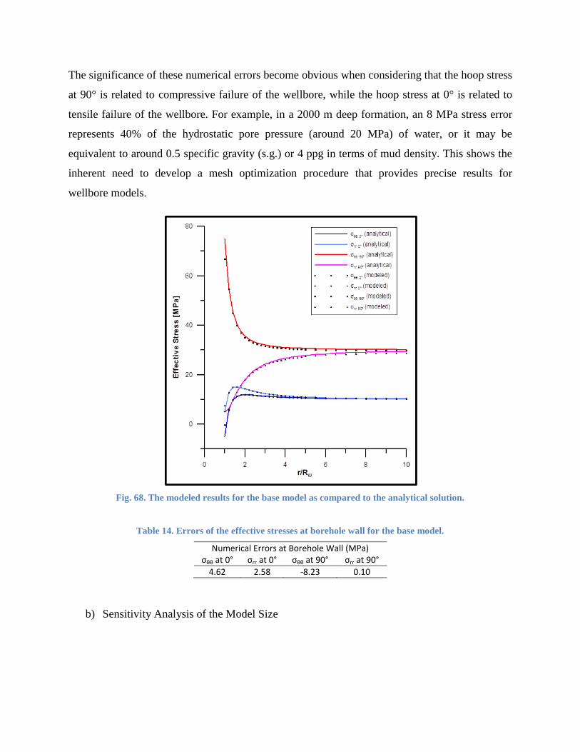
The significance of these numerical errors become obvious when considering that the hoop stress
at 90° is related to compressive failure of the wellbore, while the hoop stress at 0° is related to
tensile failure of the wellbore. For example, in a 2000 m deep formation, an 8 MPa stress error
represents 40% of the hydrostatic pore pressure (around 20 MPa) of water, or it may be
equivalent to around 0.5 specific gravity (s.g.) or 4 ppg in terms of mud density. This shows the
inherent need to develop a mesh optimization procedure that provides precise results for
wellbore models.
Fig. 68. The modeled results for the base model as compared to the analytical solution.
Table 14. Errors of the effective stresses at borehole wall for the base model.
Numerical Errors at Borehole Wall (MPa) σθθ at 0° σrr at 0° σθθ at 90° σrr at 90°
4.62 2.58 -8.23 0.10
b) Sensitivity Analysis of the Model Size
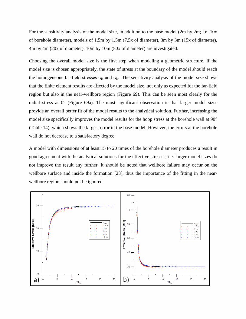
For the sensitivity analysis of the model size, in addition to the base model (2m by 2m; i.e. 10x
of borehole diameter), models of 1.5m by 1.5m (7.5x of diameter), 3m by 3m (15x of diameter),
4m by 4m (20x of diameter), 10m by 10m (50x of diameter) are investigated.
Choosing the overall model size is the first step when modeling a geometric structure. If the
model size is chosen appropriately, the state of stress at the boundary of the model should reach
the homogeneous far-field stresses σH and σh. The sensitivity analysis of the model size shows
that the finite element results are affected by the model size, not only as expected for the far-field
region but also in the near-wellbore region (Figure 69). This can be seen most clearly for the
radial stress at 0° (Figure 69a). The most significant observation is that larger model sizes
provide an overall better fit of the model results to the analytical solution. Further, increasing the
model size specifically improves the model results for the hoop stress at the borehole wall at 90°
(Table 14), which shows the largest error in the base model. However, the errors at the borehole
wall do not decrease to a satisfactory degree.
A model with dimensions of at least 15 to 20 times of the borehole diameter produces a result in
good agreement with the analytical solutions for the effective stresses, i.e. larger model sizes do
not improve the result any further. It should be noted that wellbore failure may occur on the
wellbore surface and inside the formation [23], thus the importance of the fitting in the near-
wellbore region should not be ignored.

Fig. 69. Influence of model size on the effective stresses at a) σrr at 0° and b) σθθ at 90° with respect to σH. The
larger the model size, the smaller become the errors in the near-wellbore and in the far-field region.
Table 15. Sensitivity analysis of the model size using displacement boundary conditions. The base model is
highlighted.
Model Size (m)
Numerical Errors at Borehole Wall (MPa) σθθ at 0° σrr at 0° σθθ at 90° σrr at 90°
1.75 5.02 2.55 -9.25 0.11 2 4.62 2.58 -8.23 0.10 3 4.38 2.64 -7.37 0.09 4 4.25 2.62 -7.14 0.10
10 4.14 2.63 -6.91 0.09
c) Sensitivity Analysis of the Element Type
For the sensitivity analysis of the element type, 1st (base model) and 2
nd order of quadrilateral
and 2nd
order of triangular elements are studied. 1st order triangular elements are not used here
because pore pressure cannot be applied for this element in ABAQUS.
All three types of elements yield very similar results beyond r/Rw = 2 (Figure 70). However
close to the borehole wall, i.e. r/Rw = 1 to 2, quadrilateral 2nd order element and triangular 2nd
order element both provide better results than the quadrilateral 1st order element, and the
maximum error at the borehole wall can be greatly reduced to around -1.25 (quads) or -0.13
(trias) MPa from -8.23 MPa (Table 16). Although the 2nd order triangular element produces
slightly better results than the quadrilateral 2nd order element at the borehole wall, the results
from quadrilateral 2nd elements generally have less discrepancies compared to the analytical
solution in the region of r/Rw = 1 to 2. Thus the quadrilateral 2nd
order element should be chosen
over triangular 2nd
order element to obtain an overall better fitting to the analytical solution.
Table 16. Sensitivity analysis of the element type using displacement boundary conditions. The base model is
highlighted.
Element Type
Numerical Errors at Borehole Wall (MPa) σθθ at 0° σrr at 0° σθθ at 90° σrr at 90°
1st Quad 4.62 2.58 -8.23 0.10 2nd Quad 0.50 -0.80 -1.25 0.50 2nd Tria 1.11 -0.63 -0.13 0.06

Fig. 70. Influence of element type for the hoop stress at 90°. The choice of 2nd order element greatly
increases the accuracy of the modeled result. The 2nd order quadrilateral element is slightly better than the
2nd order triangular element due to the better fitting near the wellbore surface (r/Rw = 1 to 1.5).
d) Sensitivity Analysis of the Mesh Density
For the sensitivity analysis of the mesh density in the near-wellbore region (the base model has a
mesh density of 20 elements per quarter wellbore circumference and a mesh density of 20
elements per the radial distance (4 Rw) mesh densities of 10, 30 and 40 elements per quarter
wellbore circumference and mesh densities of 10, 30, 40, 50 element per 4Rw radial distance are
studied.
A change in the circumferential mesh density has nearly no effects to the model results near the
borehole or for the overall fitting of the results in the entire model (Table 17). An increase in
mesh density would adversely cause a slightly larger error, resulting from a poorer aspect ratio of
the elements due to the elongated shape, if the radial mesh density is fixed.
A change in the radial mesh density significantly alters the model results and by utilizing higher
densities significant improvement can be obtained (Figure 71). This becomes most apparent for
the hoop stress at 90° where the difference between the model results and the analytical solution
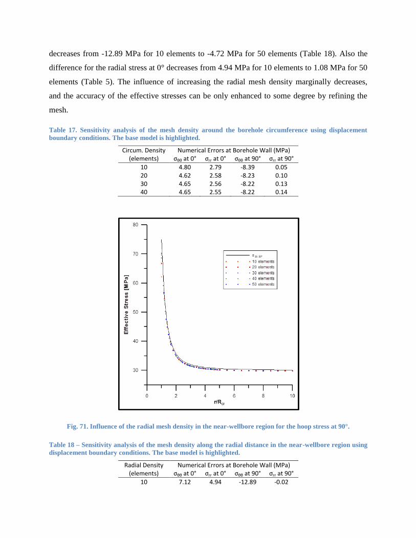
decreases from -12.89 MPa for 10 elements to -4.72 MPa for 50 elements (Table 18). Also the
difference for the radial stress at 0° decreases from 4.94 MPa for 10 elements to 1.08 MPa for 50
elements (Table 5). The influence of increasing the radial mesh density marginally decreases,
and the accuracy of the effective stresses can be only enhanced to some degree by refining the
mesh.
Table 17. Sensitivity analysis of the mesh density around the borehole circumference using displacement
boundary conditions. The base model is highlighted.
Circum. Density (elements)
Numerical Errors at Borehole Wall (MPa) σθθ at 0° σrr at 0° σθθ at 90° σrr at 90°
10 4.80 2.79 -8.39 0.05 20 4.62 2.58 -8.23 0.10 30 4.65 2.56 -8.22 0.13 40 4.65 2.55 -8.22 0.14
Fig. 71. Influence of the radial mesh density in the near-wellbore region for the hoop stress at 90°.
Table 18 – Sensitivity analysis of the mesh density along the radial distance in the near-wellbore region using
displacement boundary conditions. The base model is highlighted.
Radial Density (elements)
Numerical Errors at Borehole Wall (MPa) σθθ at 0° σrr at 0° σθθ at 90° σrr at 90°
10 7.12 4.94 -12.89 -0.02

20 4.62 2.58 -8.23 0.10 30 3.58 1.76 -6.31 0.11 40 2.95 1.34 -5.28 0.08 50 2.93 1.08 -4.72 0.07
e) General Meshing Guideline
From the sensitivity study presented for the displacement boundary conditions, a general
guideline for meshing and the choice of meshing parameters can be obtained. Finite element
meshes of borehole models should:
1) use an appropriate model size to yield a good match to the analytical solution throughout the
model;
2) use 2nd order quadrilateral elements to increase the accuracy of effective stresses at the
borehole wall;
3) use a finer mesh along the radial distance in the near-wellbore region to further improve the
results;
4) use an appropriate mesh density along the borehole circumference to ensure a good aspect
ratio of the elements.
2.1.5.2.Mesh Optimization
According to the parametric study and the guideline obtained above, an optimized model is
constructed using the following parameters:
• Model size: 4m by 4m, which is 20x the borehole diameter.
• 2nd order quadrilateral element.
• Radial mesh density in the near-wellbore region: 40 elements along the 4Rw distance.
• Circumferential density in the near-wellbore region: 40 elements per quarter wellbore
circumference.

Comparing the numerical results from the optimized model to the analytical solution shows a
very good agreement (Figure 72). Further the error at the borehole wall is minimized to less than
0.5 MPa (Table 19).
Fig. 72. The modeled results from the optimized model compared with the analytical results.
Table 19. Errors of the modeled results from the optimized model compared to that of the base model.
Model Numerical Errors at Borehole Wall (MPa) σθθ at 0° σrr at 0° σθθ at 90° σrr at 90°
Base 4.62 2.58 -8.23 0.10 Optimized 0.09 -0.29 -0.28 0.50
2.1.5.3.Stress Boundary Conditions and Drilling Simulation Boundary Conditions
The sensitivity analyses for the stress boundary conditions and the drilling process simulation
boundary conditions yield very similar results as for the displacement boundary conditions.
Therefore, the majority of this data is not repeatedly shown here again. The comparison of the
base model case using the three boundary condition scenarios is shown in Figure 73. While the
stress boundary conditions seem to provide the best solution at the borehole wall, especially for

the hoop stress at 90° (Table 20), the discrepancies at distances larger than r/Rw = 1.2 become
larger. The mean error and the standard deviation of the error of the hoop stress at 90° between
1.2≤ r/Rw ≤2 for the stress boundary conditions are 1.04 MPa and 0.55MPa, respectively,
compared to -0.53 MPa (mean error) and 0.13 MPa (standard deviation) for both displacement
boundary conditions and for drilling simulation boundary conditions. Further, the stress
boundary conditions show relatively large discrepancies for the sensitivity check on the model
size. The hoop stress at 0° at the model boundary does not converge to the far-field stress, and
only slightly improves with increasing model size (Figure 74).
Due to the similarity of the sensitivity analysis for all the three boundary conditions the same
meshing guideline can be applied and an optimized model according to our suggestion above can
be obtained. In the optimized model the results for each boundary condition scenario are
improved. In contrast to the base model, after optimization, the displacement boundary
conditions and the drilling simulation boundary conditions now yield the smallest errors also at
the borehole wall (Table 20) and are thus preferred over the stress boundary conditions. It should
be noted that the drilling simulation boundary conditions increase the numerical complexity by
their implementation and thus displacement boundary conditions are recommended for wellbore
stress analyses.
Table 20. Errors at the wellbore surface for the base model and the optimized model under three boundary
conditions.
Model Numerical Errors at Borehole Wall (MPa) σθθ at 0° σrr at 0° σθθ at 90° σrr at 90°
Base Displace 4.62 2.58 -8.23 0.10 Stress 3.11 2.71 -5.28 0.05 Drilling Sim 4.67 2.59 -8.23 0.10
Optimized Displace 0.09 -0.29 -0.25 -0.50 Stress 0.40 0.30 0.60 0.51 Drilling Sim 0.08 -0.29 -0.25 0.50

Fig. 73. Base model under three boundary conditions and compared to the analytical solutions.

Fig. 74. Hoop stress at 0° for the stress boundary conditions shows a great discrepancy near the model
boundary for the base model.
2.1.6. Discussion
2.1.6.1.Models Using the Displacement Boundary Conditions
The numerical study presented in this paper shows that, considering the general availability of
numerical modeling tools such as the finite element (FE) method, care has to be taken when
these methods are applied for wellbore stress analysis. It is obvious that for the case of a
homogeneous, isotropic, linear elastic material the analytical solution provides the accurate
solution and numerical analysis is not necessary. However, many applications for wellbore
stability or hydraulic fracturing occur in anisotropic rocks (e.g. shale; [24]) or require composite
materials (e.g. cementing analysis; [25]) where analytical solutions do not exist. Therefore,
numerical wellbore stress analysis for a homogeneous, isotropic, linear elastic material provides
an excellent opportunity to test the influence of the various discretization parameters on the
existing analytical solution [3] and to provide conclusions for meshing and model optimization
requirements for all types of wellbore stress analyses. A variety of studies have shown that the
accuracy of results of FE studies are highly dependent on discretization approaches and
parameters [26, 27, 28]. Even if errors of the modeled results are within 1 to 3 MPa [10], these

should be taken seriously, otherwise the subsequent study based on the modeled results might be
questionable.
Our study shows that the most prominent improvement on the accuracy of the modeled result is
obtained by using 2nd order elements. The -8.23 MPa error of the hoop stress at 90° in the base
model using the displacement boundary is decreased to around 1 MPa by merely changing the
element type with other modeling parameters fixed, and at no cost to the increase of the numbers
of the elements, although more nodes are used. In the sensitivity analysis, the increase of radial
mesh density in the near wellbore region the error is reduced to around 5 MPa, and its influence
marginally diminishes. Thus choosing 2nd
order elements has the highest priority before the
increase of mesh density.
In the context of the significance of the numerical errors, it should be noted that the FE method
inherently introduces errors as it is a method of approximation [8]. This becomes most evident
when comparing the stress results at the borehole wall, where the numerical model yields the
largest error. One has to understand that the FE method calculates stresses at the element
integration point [29], which is situated inside the element (Figure 75) and thus cannot reproduce
the absolute exact result at free surfaces like the borehole wall. To compare FE model stresses to
the analytical solution the element stresses from the integration points have to be extrapolated to
the nodal coordinates (Figure 75). This procedure generally provides very accurate agreements
for nodes attached to 4 elements but at the free surface of the borehole wall an error is
introduced. Here, the stress changes rapidly and the stress at this node is extrapolated from the
two integration points inside the formation only. This extrapolation will always return a non zero
stress value for the radial stress (if no fluid pressure is applied) and thus cannot obey the rule that
normal stresses do not exist at a free surface.

Fig. 75. Stresses are calculated at the element integration points [29]. When stresses are extrapolated to nodal
positions a greater error is introduced especially near the borehole wall.
2.1.6.2.Comparisons of the Models for the Different Boundary Conditions
The displacement and drilling simulation boundary conditions produce almost identical results
and yield smaller errors than the stress boundary conditions. Since the drilling simulation
boundary conditions require an additional initial pre-stressing procedure, displacement boundary
conditions are considered sufficient for wellbore stress analyses if there is no specific need for
simulating the drilling process.
2.1.6.3.Implications for Safe Mud Weight Prediction
In order to demonstrate the significance of the numerical errors for wellbore stability
applications we predict the safe mud weight window for the base model, the optimized model,
and for the analytical solution under three different stress regimes: normal or extensional faulting
(NF), strike-slip (SS) faulting, and compressional or reverse faulting (RF) regime. It should be
noted again that the evaluation of an appropriate failure criterion for wellbore stability analyses
is beyond the scope of this paper and that each failure criterion is affected differently by the
numerical errors. We use the Mohr-Coulomb failure criterion as the most conservative [16]
criterion for this analysis to point out the general implications for wellbore stability.
Borehole Wall
Stress calculated at integration point
Nodal stress extrapolated from integration point
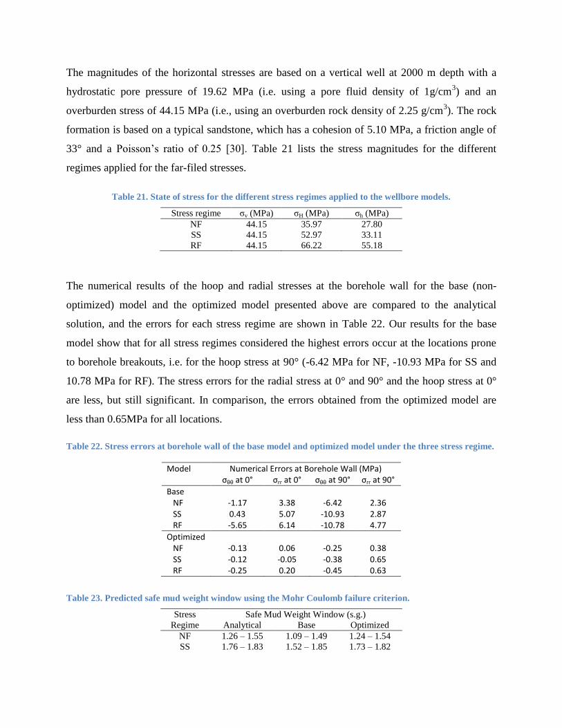
The magnitudes of the horizontal stresses are based on a vertical well at 2000 m depth with a
hydrostatic pore pressure of 19.62 MPa (i.e. using a pore fluid density of 1g/cm3) and an
overburden stress of 44.15 MPa (i.e., using an overburden rock density of 2.25 g/cm3). The rock
formation is based on a typical sandstone, which has a cohesion of 5.10 MPa, a friction angle of
33° and a Poisson’s ratio of 0.25 [30]. Table 21 lists the stress magnitudes for the different
regimes applied for the far-filed stresses.
Table 21. State of stress for the different stress regimes applied to the wellbore models.
Stress regime σv (MPa) σH (MPa) σh (MPa)
NF 44.15 35.97 27.80
SS 44.15 52.97 33.11
RF 44.15 66.22 55.18
The numerical results of the hoop and radial stresses at the borehole wall for the base (non-
optimized) model and the optimized model presented above are compared to the analytical
solution, and the errors for each stress regime are shown in Table 22. Our results for the base
model show that for all stress regimes considered the highest errors occur at the locations prone
to borehole breakouts, i.e. for the hoop stress at 90° (-6.42 MPa for NF, -10.93 MPa for SS and
10.78 MPa for RF). The stress errors for the radial stress at 0° and 90° and the hoop stress at 0°
are less, but still significant. In comparison, the errors obtained from the optimized model are
less than 0.65MPa for all locations.
Table 22. Stress errors at borehole wall of the base model and optimized model under the three stress regime.
Model Numerical Errors at Borehole Wall (MPa) σθθ at 0° σrr at 0° σθθ at 90° σrr at 90°
Base NF -1.17 3.38 -6.42 2.36 SS 0.43 5.07 -10.93 2.87 RF -5.65 6.14 -10.78 4.77
Optimized NF -0.13 0.06 -0.25 0.38 SS -0.12 -0.05 -0.38 0.65 RF -0.25 0.20 -0.45 0.63
Table 23. Predicted safe mud weight window using the Mohr Coulomb failure criterion.
Stress
Regime
Safe Mud Weight Window (s.g.)
Analytical Base Optimized
NF 1.26 – 1.55 1.09 – 1.49 1.24 – 1.54
SS 1.76 – 1.83 1.52 – 1.85 1.73 – 1.82
RF 1.99 – 4.19 1.68 – 4.01 1.96 – 4.18
Predicting the safe mud weight window from the modeled results shows that the collapse
pressure gradient and the breakdown pressure gradient for the optimized model have a maximum
error of -0.03 specific gravity (s.g.) or -0.25 ppg. This error is within the practical limits of mud
weight density control.
However, if the safe mud weight window for the base (non-optimized) model is predicted (for all
three stress regimes), the errors become significant. For the collapse pressure gradient the model
yields a much lower collapse pressure compared to the analytical solution. With errors of -0.17, -
0.24, and -0.31 s.g. (or 1.4, 2.0, and 2.6 ppg) for NF, SS, and RF regimes, respectively, this
would lead to an over-optimistic prediction for the mud weight. If this error was neglected mud
weights causing borehole breakouts might be chosen.
This is most noticeable for the strike-slip regime where vertical wells represent the least stable
well direction. For the example case the analytical solution shows that the safe mud weight
window is very narrow (1.76 to 1.83 s.g. or 14.67 to 15.23 ppg), while the non-optimized model
results predict a mud weight window of 1.57 to 1.85 s.g. or 13.05 to 15.43 ppg. This clearly
overestimates the range of actual applicable mud weights and a stable borehole cannot be
guaranteed.
The breakdown pressure is determined by the hoop stress at 0°. Though the base model only
yields an error of 0.02 s.g. of the breakdown pressure gradient in the slip-strike stress regime, the
breakdown pressure for the normal faulting and reverse faulting regime shows significant errors
of -0.06 and -0.18 s.g. (or 0.5 and 1.5 ppg), respectively. Such errors are of less importance for
the reverse faulting regime because the safe mud weight window is rather wide. However, for
hydraulic fracturing applications the error accounts for an underestimation of 1.5 ppg of the
fracture gradient.
Although only the Mohr-Coulomb failure criterion is used in the wellbore stability analysis, this
study shows that the choice of boundary conditions and meshing parameters has crucial
implications to the applications of wellbore stress analyses.

2.1.7. Conclusions
The use of finite element analysis in geomechanics provides an excellent tool for complex
problems where analytical solutions do not exist. For the case of wellbore stress analyses the
accuracy of the numerical results at the borehole wall and in its direct vicinity ensures the
applicability of these results to wellbore stability, wellbore design, and cementing analyses, as
well as hydraulic fracturing processes.
Our study shows that boundary conditions and meshing parameters, i.e. model size, element type
and mesh density in the near-wellbore region, have a significant influence on the accuracy of
results and if not appropriately chosen, the effective stresses in the near-wellbore region show
significant errors (as high as 11 MPa) when compared to the analytical solution. This misfit
shows the inherent need to conduct a mesh optimization for numerical wellbore stress analyses to
minimize the errors. For 2D wellbore stress analyses, displacement boundary conditions provide
the best fit to the analytical solution for both the near-wellbore region and the far-field. The use
of 2nd order quadrilateral elements and a relatively fine mesh in the near-wellbore region are of
first priority to obtain accurate results. Further, the overall model size has to be chosen carefully.
With the meshing guideline presented in this study, a good match to the analytical solution
throughout the model can be obtained and the error at the borehole wall and in the near-wellbore
region can be minimized. It is expected that this general modeling technique also applies to more
complex models. If discretization parameters are not optimized, the modeled results are of
question and the subsequent analysis should not be relied on.
This conclusion becomes evident for the case of an exemplary wellbore stability analysis in this
study. Predicted safe mud weight windows from a non-optimized model for three different stress
regimes show differences of up to -0.24 s.g. or 2.6 ppg compared to the analytical solution. For
the cases presented this may specifically lead to a significant misinterpretation of the minimum
usable mud weight and borehole collapse may result.

2.2.Wellbore Stability Analysis
2.2.1. Pressure Window
The pressure window used for this analysis consists of three unique curves. The first of these
curves is the pore pressure. Pore pressure is the pressure exerted by trapped water molecules in
the pores of the rock. For the purposes of this study the pore pressure is considered to be
hydrostatic and is calculated using the following equation:
(16)
where ρw is the density of water; g is the acceleration due to gravity; and z is the depth of
interest.
The other two curves used to define the pressure window are the collapse pressure (shear failure)
and the fracture gradient (tensile failure). The collapse pressure is the minimum pressure which
must be maintained in the wellbore before the onset of borehole collapse. It is reached when the
hoop stress reaches the compressive strength of the rock. The collapse pressure is determined by
using a Mohr-Coulomb failure criterion and the assumption that the mean stress is constant at
any one point in the wellbore. The fracture gradient is the maximum pressure which can be
sustained in the wellbore before the surrounding rock begins to undergo tensile failure
(fractures). Tensile failure occurs when the hoop stress in the wellbore is less than the tensile
strength of the rock. Both types of failure can be detrimental to the drilling of a well so a
thorough knowledge of the pressure window is important.
2.2.2. Vertical Wellbores
The reservoir scale Finite Element Model (FEM) has been used to determine the placement of
three vertical wellbores for the different stress regimes. The wellbores in question were placed at
the crest of the anticline, the base of the anticline, and the limb of the anticline (Figure 76).
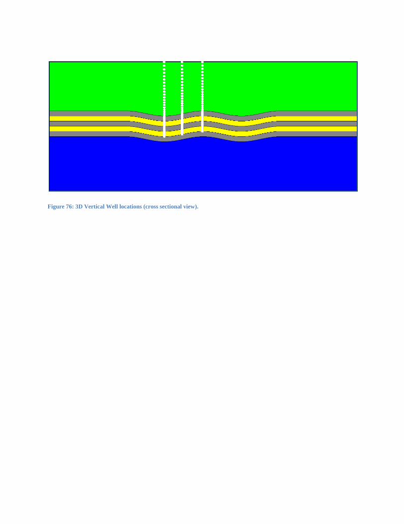
Figure 76: 3D Vertical Well locations (cross sectional view).
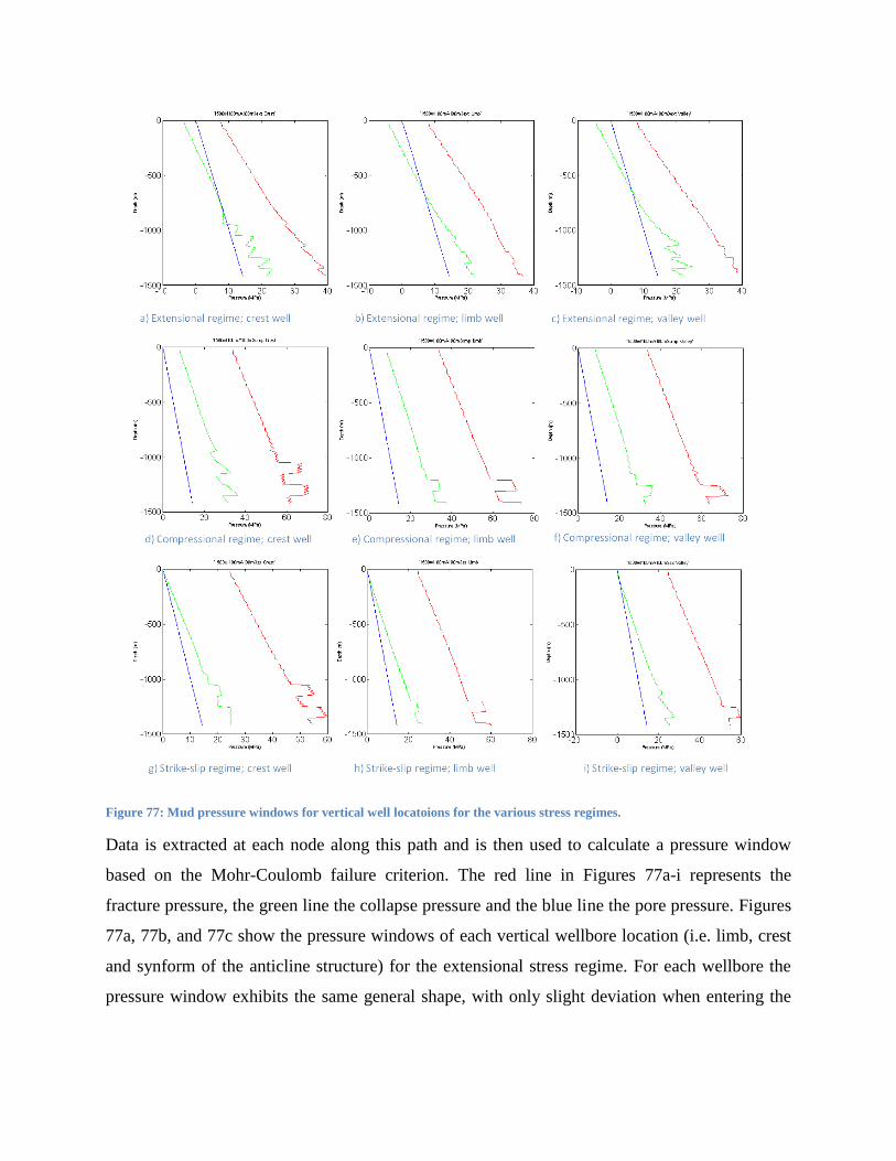
Figure 77: Mud pressure windows for vertical well locatoions for the various stress regimes.
Data is extracted at each node along this path and is then used to calculate a pressure window
based on the Mohr-Coulomb failure criterion. The red line in Figures 77a-i represents the
fracture pressure, the green line the collapse pressure and the blue line the pore pressure. Figures
77a, 77b, and 77c show the pressure windows of each vertical wellbore location (i.e. limb, crest
and synform of the anticline structure) for the extensional stress regime. For each wellbore the
pressure window exhibits the same general shape, with only slight deviation when entering the
reservoir layer. For this regime the pressures at the bottom of the wellbore differ by about
10MPa.
Figures 77d, 77e, and 77f show the pressure windows of each wellbore for the compressional
stress regime. In general the compressional regime shows a much larger mud window compared
to the extensional models.
Figures 77g, 77h, and 77i show the pressure windows of each wellbore for the strike-slip stress
regime. The pressure window is similar to the compressional regime, however at the crest
location the strike sip stress regime shows the overall widest pressure window.
As an initial conclusion vertical wells are safe to drill for the generic anticline models. However
to provide more general wellbore stability criteria applicable for more complex scenarios
deviated wellbores of type I & II wells are additionally investigated. Type I inclined wellbores
become relevant as the trajectory has an increased surface area with the injection layer thus
increasing infectivity. A more detailed description and the numerics of these well types are given
in Appendix 2.
2.2.3. Deviated Wellbores
A deviated wellbore is any wellbore which does not lie entirely along the vertical axis [2].
Deviated wellbores are defined by an angle of inclination (i) and an azimuthal angle (α) (Figure
78). The angle of inclination is the deviation of the wellbore from the vertical axis and ranges
from 0o-90
o. The azimuthal angle is the direction of the borehole axis with respect to north. The
azimuth ranges from 0o-360
o where 0
o is north and the angle increases clockwise [7, 9].
Two unique types of well profiles will be tested in this study (Figure 79). A Type I well profile
consists of a vertical well section that extends downwards from surface until it reaches the
kickoff point [KOP]. Once the KOP is achieved the well enters a build section until the final
inclination angle is achieved. The well then holds this angle until it reaches the target. A Type II
well profile consists of a vertical section down to the KOP. After the KOP is reached the well
extends into a build section until it reaches the desired inclination angle. Once the desired
inclination angle is obtained, the angle will be held until the well reaches a desired length. At this
length, the well enters a drop section (drop off point; DOP) until it reaches the reservoir or
another hold section.
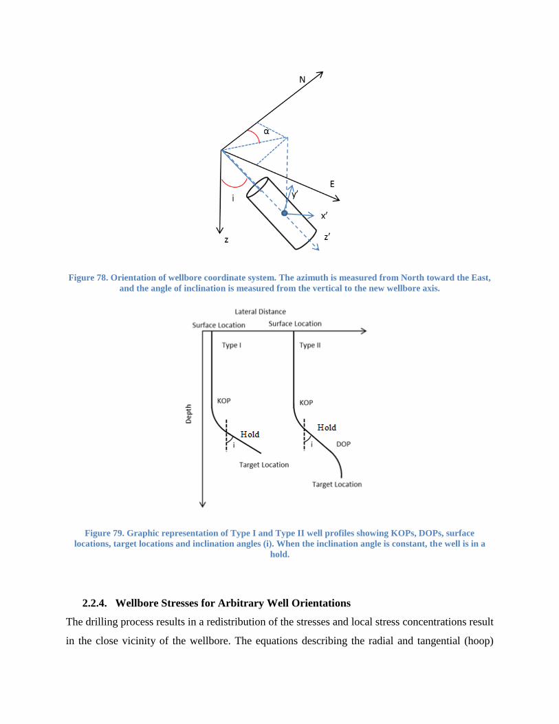
Figure 78. Orientation of wellbore coordinate system. The azimuth is measured from North toward the East,
and the angle of inclination is measured from the vertical to the new wellbore axis.
Figure 79. Graphic representation of Type I and Type II well profiles showing KOPs, DOPs, surface
locations, target locations and inclination angles (i). When the inclination angle is constant, the well is in a
hold.
2.2.4. Wellbore Stresses for Arbitrary Well Orientations
The drilling process results in a redistribution of the stresses and local stress concentrations result
in the close vicinity of the wellbore. The equations describing the radial and tangential (hoop)
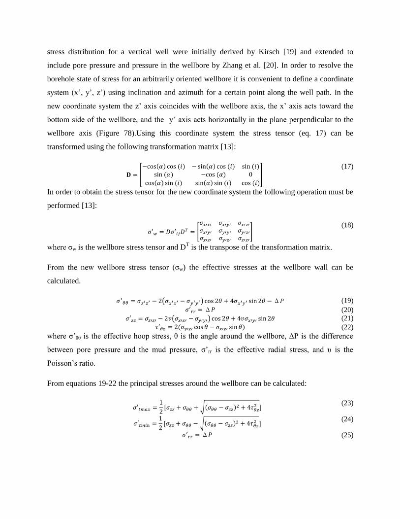
stress distribution for a vertical well were initially derived by Kirsch [19] and extended to
include pore pressure and pressure in the wellbore by Zhang et al. [20]. In order to resolve the
borehole state of stress for an arbitrarily oriented wellbore it is convenient to define a coordinate
system (x’, y’, z’) using inclination and azimuth for a certain point along the well path. In the
new coordinate system the z’ axis coincides with the wellbore axis, the x’ axis acts toward the
bottom side of the wellbore, and the y’ axis acts horizontally in the plane perpendicular to the
wellbore axis (Figure 78).Using this coordinate system the stress tensor (eq. 17) can be
transformed using the following transformation matrix [13]:
(17)
In order to obtain the stress tensor for the new coordinate system the following operation must be
performed [13]:
(18)
where σw is the wellbore stress tensor and DT is the transpose of the transformation matrix.
From the new wellbore stress tensor (σw) the effective stresses at the wellbore wall can be
calculated.
(19)
(20)
(21)
(22)
where σ’θθ is the effective hoop stress, θ is the angle around the wellbore, ΔP is the difference
between pore pressure and the mud pressure, σ’rr is the effective radial stress, and υ is the
Poisson’s ratio.
From equations 19-22 the principal stresses around the wellbore can be calculated:
(23)
(24)
(25)
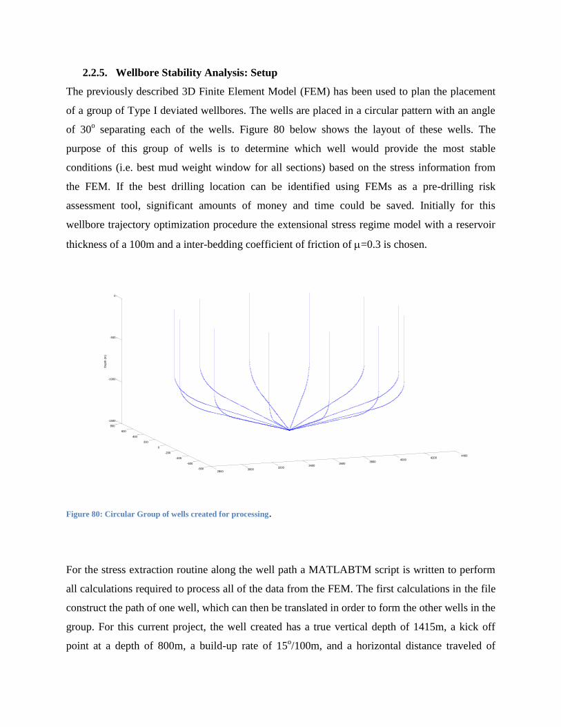
2.2.5. Wellbore Stability Analysis: Setup
The previously described 3D Finite Element Model (FEM) has been used to plan the placement
of a group of Type I deviated wellbores. The wells are placed in a circular pattern with an angle
of 30o separating each of the wells. Figure 80 below shows the layout of these wells. The
purpose of this group of wells is to determine which well would provide the most stable
conditions (i.e. best mud weight window for all sections) based on the stress information from
the FEM. If the best drilling location can be identified using FEMs as a pre-drilling risk
assessment tool, significant amounts of money and time could be saved. Initially for this
wellbore trajectory optimization procedure the extensional stress regime model with a reservoir
thickness of a 100m and a inter-bedding coefficient of friction of =0.3 is chosen.
Figure 80: Circular Group of wells created for processing.
For the stress extraction routine along the well path a MATLABTM script is written to perform
all calculations required to process all of the data from the FEM. The first calculations in the file
construct the path of one well, which can then be translated in order to form the other wells in the
group. For this current project, the well created has a true vertical depth of 1415m, a kick off
point at a depth of 800m, a build-up rate of 15o/100m, and a horizontal distance traveled of
28003000
32003400
36003800
40004200
4400
-800
-600
-400
-200
0
200
400
600
800
-1500
-1000
-500
0
Depth
(m
)

718m. All of the other wells have the same initial data as this well, but are shifted 30o from one
another (Figure 80). Once all of the wells are created, the file will then use the coordinate and
stress data and extract a cylinder of data which encompasses all of the wells; i.e. all stress data
not containing a well path is discarded. This step is necessary to significantly cut down
computation time. Figure x shows the created smoothed well paths (blue) and the matched data
wells (red). It should be noted here that the angle for the well deviation is taken from the smooth
trajectory (Figure 81, blue line) and the stress input is taken from the nearest node (Figure 81,
red line). By having new wells which have the exact coordinates as nodes in our model, we are
then able to export all of the stress data at those coordinates for post processing.
Figure 81: Both created and matched data wells.
Extracting all of the stress tensors at each node of our well from the FEM, we then use the
previously reported method of stress transformation to transform the stress tensors from the
geographic system to the system of each of our wellbores. A difference is made concerning the
definition of the azimuth used. For this portion of the projected, we have defined the azimuth to
be the angle of the well measured clockwise from geographic North. The figure below shows
how the azimuth has been defined.
2800
3000
3200
3400
3600
3800
4000
4200
4400
-800-600
-400-200
0200
400600
800
-1500
-1000
-500
0
Depth
(m
)
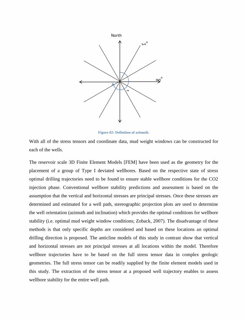
Figure 82: Definition of azimuth.
With all of the stress tensors and coordinate data, mud weight windows can be constructed for
each of the wells.
The reservoir scale 3D Finite Element Models [FEM] have been used as the geometry for the
placement of a group of Type I deviated wellbores. Based on the respective state of stress
optimal drilling trajectories need to be found to ensure stable wellbore conditions for the CO2
injection phase. Conventional wellbore stability predictions and assessment is based on the
assumption that the vertical and horizontal stresses are principal stresses. Once these stresses are
determined and estimated for a well path, stereographic projection plots are used to determine
the well orientation (azimuth and inclination) which provides the optimal conditions for wellbore
stability (i.e. optimal mud weight window conditions; Zoback, 2007). The disadvantage of these
methods is that only specific depths are considered and based on these locations an optimal
drilling direction is proposed. The anticline models of this study in contrast show that vertical
and horizontal stresses are not principal stresses at all locations within the model. Therefore
wellbore trajectories have to be based on the full stress tensor data in complex geologic
geometries. The full stress tensor can be readily supplied by the finite element models used in
this study. The extraction of the stress tensor at a proposed well trajectory enables to assess
wellbore stability for the entire well path.
α
North 0
o
90o
30o

In order to determine and assess the most stable well trajectory for the anticline geometries in
this study, the proposed wells were placed in a circular pattern with an angle of 30o separating
each of the wells. Table 24 shows the input data which was used to create the 15 well paths. This
study is independent of well inclination changes. The procedure to create the wells was given in
the progress report for quarter 3. Figure 81 above shows the layout of these wells (blue) and the
matched data from the model (red). The purpose of defining a circle of wells is to determine
which well represents the most stable conditions within the respective state of stress.
2.2.6. Wellbore Stability Analysis: Model Validation
A simplified FEM has been setup to validate and verify the wellbore trajectory calculation and
pressure window calculation procedure. The model is a simple block model which was used to
perform a statistical analysis of the MATLABTM script file. The purpose of the analysis is to
compare the stresses and mud pressures calculated for the wellbore trajectories to the analytical
solution. The model setup is shown below in Figure 83. This model is in a simple all sandstone
block in an extensional stress regime where the vertical stress is the maximum principal stress
and the two horizontal stresses are equal in magnitude and are the intermediate and minimum
principal stresses. For this model the pore pressure is hydrostatic. Two well paths, one vertical
and one with an inclination of 45 degrees from horizontal, were created in order to perform the
analysis. The values used in the analysis of these wells are in Table 24 below.
Table 24. Input data for the validation model vertical and deviated well path.
Solution Type Depth (m) S11 (Mpa) S22 (Mpa) S33 (Mpa) S12 (Mpa) S13 (Mpa) S23 (Mpa) Pp (Mpa) Azimuth (o) Inclination (o)
Analytical 2500 40.29 40.29 61.31 0 0 0 24.53 0 0
MATLAB 2490 40.14 40.14 61.08 ~0 ~0 ~0 24.44 0 0
Solution Type Depth (m) S11 (Mpa) S22 (Mpa) S33 (Mpa) S12 (Mpa) S13 (Mpa) S23 (Mpa) Pp (Mpa) Azimuth (o) Inclination (o)
Analytical 2500 40.29 40.29 61.31 0 0 0 24.53 30 45
MATLAB 2490 40.14 40.14 61.08 ~0 ~0 ~0 24.44 30 44.99
Model Data for Vertical Well
Model Data for Deviated Well
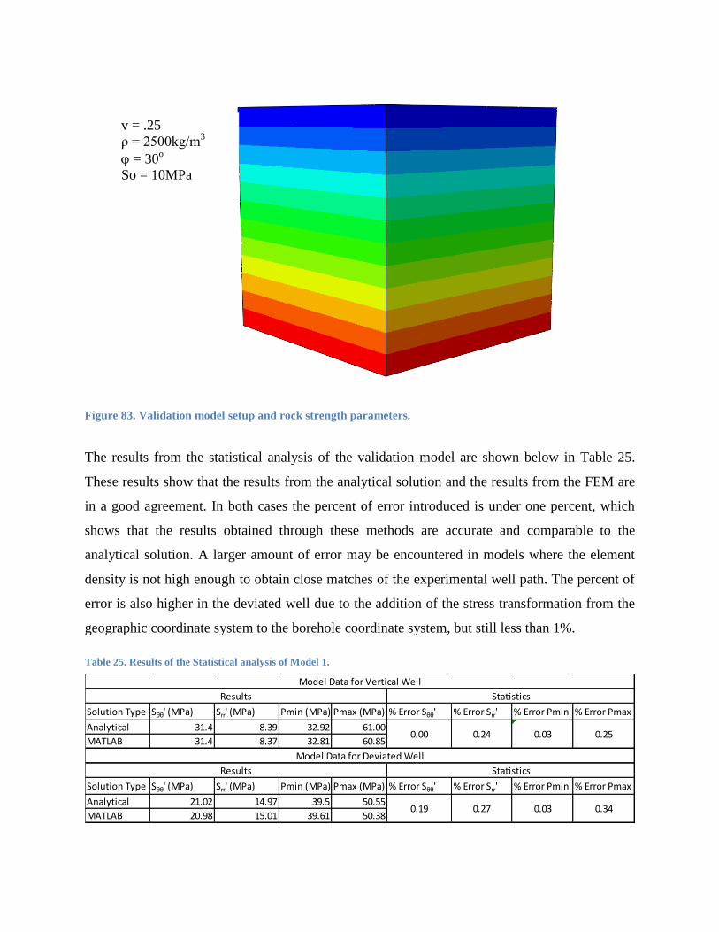
Figure 83. Validation model setup and rock strength parameters.
The results from the statistical analysis of the validation model are shown below in Table 25.
These results show that the results from the analytical solution and the results from the FEM are
in a good agreement. In both cases the percent of error introduced is under one percent, which
shows that the results obtained through these methods are accurate and comparable to the
analytical solution. A larger amount of error may be encountered in models where the element
density is not high enough to obtain close matches of the experimental well path. The percent of
error is also higher in the deviated well due to the addition of the stress transformation from the
geographic coordinate system to the borehole coordinate system, but still less than 1%.
Table 25. Results of the Statistical analysis of Model 1.
Solution Type Sθθ' (MPa) Srr' (MPa) Pmin (MPa) Pmax (MPa) % Error Sθθ' % Error Srr' % Error Pmin % Error Pmax
Analytical 31.4 8.39 32.92 61.00
MATLAB 31.4 8.37 32.81 60.85
Solution Type Sθθ' (MPa) Srr' (MPa) Pmin (MPa) Pmax (MPa) % Error Sθθ' % Error Srr' % Error Pmin % Error Pmax
Analytical 21.02 14.97 39.5 50.55
MATLAB 20.98 15.01 39.61 50.38
Model Data for Deviated Well
Results Statistics
0.19 0.27 0.03 0.34
Model Data for Vertical Well
Results Statistics
0.00 0.24 0.03 0.25
v = .25
ρ = 2500kg/m3
= 30o
So = 10MPa
2.2.7. Wellbore Stability Analysis: Stress Regimes
For the wellbore stability analysis of the generic anticline structure three different stress regimes
have been investigated: extensional [Model 2], compressional [Model 3], and strike-slip [Model
4]. In each of these models 15 well locations were created and analyzed. The geometry and rock
parameters used in Models 2, 3, 4, 5, and 6 are shown in Figure 4. Models 2, 3, and 4 were all
created with a coefficient of friction of 0.3 on the rock contact surfaces.
Two additional models were created in order to test the influence of inter-bedding friction in the
pressure windows. Each of these models was created using the same anticline geometry as
models 2, 3, and 4, but the only stress regime which was tested was the compressional regime.
The coefficients of friction were tested are 0.1 [Model 5] and 0.8 [Model 6].
2.2.7.1.Extensional Stress Regime
The 15 pressure windows which were created from Model 2 are compiled in Appendix 3.1. By
using the pressure windows and the knowledge of the intermediate principal stress direction, the
optimal drilling directions can be determined for this model. The intermediate principal stress
direction is usually the least safe drilling direction because the differential stress is the largest.
Figure 84 below shows a visualization of the intermediate stress direction for Model 2.

Figure 84. Intermediate stress direction in Model 2.
From Figure 84 the least safe drilling direction in this stress regime is highly influenced by the
geometry and boundary conditions. At the surface of the model the least safe direction is on the y
axis, but then changes to the vertical direction after about 100m. The least safe direction at the
reservoir would be a completely horizontal well along the x axis. The same trends can be seen
from the figures in Appendix 3. The smallest sections of the pressure windows are at the surface
where the pore pressure has become the minimum safe mud weight for drilling. If the windows
are examined as a whole, with the target as the main point of interest, it can be seen that as the
azimuthal angle approaches either 90 or 270 degrees the pressure window narrows more than it
does at other angles. By inspection it can be seen that as the azimuthal angle approaches angles
of either 0 or 180 degrees the pressure window gets wider. Figure 85a below shows the pressure
window at an azimuth of 0 degrees, while Figure 85b shows the pressure window at an azimuth
of 90 degrees. In all of the pressure window figures given in this report the blue line is pore
pressure, the green line is the collapse pressure, and the red line is the fracture gradient.
Figure 85: Pressure window for Azimuth = 0oand 90o.
Figure 85a represents the best and Figure 85b the least favorable drilling directions for Model 2.
The pressure window at 0 degrees is wider and at a steeper angle, which will lessen the amount
of casing points needed. It should be noted that both wells can be drilled safely, however the
costs associated to casing will be different. The minimum casing points which a well at 0 degrees
could be safely drilled with is 2, while it would take at least 3 if not 4 casing points to drill a well
at an azimuth of 90 degrees. If drilling were to be done in this Model the best direction would
either be at 0 or 180 degrees, but there may still be slight drilling problems near the surface
where all of the wells would be vertical and would be being drilled in least safe drilling direction.
Wells drilled in directions of 90 or 270 degrees should be avoided in this Model.
2.2.7.2.Compressional Stress Regime
The resulting pressure windows for Model 3 have been compiled in Appendix 3.2. Figure 86
below shows the intermediate principal stress direction for Model 3 which does not change
throughout the length of the wells which are used in this analysis. The intermediate stress
direction is at a constant path along the y axis until the base layer of the model where the stress is
along the z axis.
-20 0 20 40 60-1500
-1000
-500
0
Pressure (MPa)
Depth
(m
)
'1500wl100mA100m3extAzimuth=90
-10 0 10 20 30 40-1500
-1000
-500
0
Pressure (MPa)
Depth
(m
)
'1500wl100mA100m3extAzimuth=0
a) b)
Figure 86. Intermediate principal stress direction for Model 3.
For Model 3 the vertical stress is not the intermediate stress near the surface or in the reservoir,
therefore vertical wells and the vertical portion of deviated wells are much safer than they were
in Model 2. The pore pressure does never become the minimum pressure for safe drilling. All of
the pressure windows for this model are relatively safe and the slope of the pressure lines
indicates that all wells could potentially be drilled with only 1 or 2 casing points.
By inspection of figures B1-B15 in Appendix 3 it can be seen that wells with an azimuth of 0 or
180 degrees, while still representing stable drilling conditions) represent the least favorable
drilling orientations. The fracture gradient in these wells narrows significantly towards the
collapse pressure causing a much smaller pressure window. As the well paths azimuths move
closer to 90 and 270 degrees the fracture gradient increases causing a larger pressure window
and a safer drilling scenario. If drilling a well in this Model, the azimuths of 90 and 270 degrees
would be the preferred well orientation. The extra space in the pressure window allows for easier
drilling, and these wells could be drilled with fewer casing points as opposed to wells drilled
along the other azimuths.
Figure 86a shows the pressure window for a well drilled along an azimuth of 0 degrees, while
Figure 86b shows the pressure window for a well drilled along an azimuth of 90 degrees. From
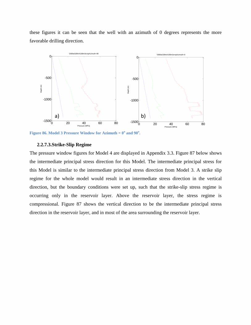
these figures it can be seen that the well with an azimuth of 0 degrees represents the more
favorable drilling direction.
Figure 86. Model 3 Pressure Window for Azimuth = 0o and 90
o.
2.2.7.3.Strike-Slip Regime
The pressure window figures for Model 4 are displayed in Appendix 3.3. Figure 87 below shows
the intermediate principal stress direction for this Model. The intermediate principal stress for
this Model is similar to the intermediate principal stress direction from Model 3. A strike slip
regime for the whole model would result in an intermediate stress direction in the vertical
direction, but the boundary conditions were set up, such that the strike-slip stress regime is
occurring only in the reservoir layer. Above the reservoir layer, the stress regime is
compressional. Figure 87 shows the vertical direction to be the intermediate principal stress
direction in the reservoir layer, and in most of the area surrounding the reservoir layer.
0 20 40 60 80-1500
-1000
-500
0
Pressure (MPa)
Depth
(m
)
'1500wl100mA100m3cmpAzimuth=90
0 20 40 60 80-1500
-1000
-500
0
Pressure (MPa)D
epth
(m
)
'1500wl100mA100m3cmpAzimuth=0
a) b)
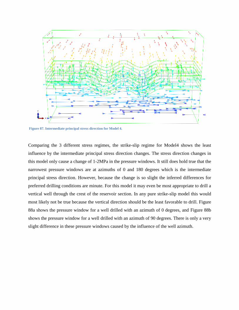
Figure 87. Intermediate principal stress direction for Model 4.
Comparing the 3 different stress regimes, the strike-slip regime for Model4 shows the least
influence by the intermediate principal stress direction changes. The stress direction changes in
this model only cause a change of 1-2MPa in the pressure windows. It still does hold true that the
narrowest pressure windows are at azimuths of 0 and 180 degrees which is the intermediate
principal stress direction. However, because the change is so slight the inferred differences for
preferred drilling conditions are minute. For this model it may even be most appropriate to drill a
vertical well through the crest of the reservoir section. In any pure strike-slip model this would
most likely not be true because the vertical direction should be the least favorable to drill. Figure
88a shows the pressure window for a well drilled with an azimuth of 0 degrees, and Figure 88b
shows the pressure window for a well drilled with an azimuth of 90 degrees. There is only a very
slight difference in these pressure windows caused by the influence of the well azimuth.
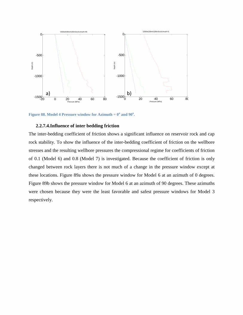
Figure 88. Model 4 Pressure window for Azimuth = 0o and 90
o.
2.2.7.4.Influence of inter bedding friction
The inter-bedding coefficient of friction shows a significant influence on reservoir rock and cap
rock stability. To show the influence of the inter-bedding coefficient of friction on the wellbore
stresses and the resulting wellbore pressures the compressional regime for coefficients of friction
of 0.1 (Model 6) and 0.8 (Model 7) is investigated. Because the coefficient of friction is only
changed between rock layers there is not much of a change in the pressure window except at
these locations. Figure 89a shows the pressure window for Model 6 at an azimuth of 0 degrees.
Figure 89b shows the pressure window for Model 6 at an azimuth of 90 degrees. These azimuths
were chosen because they were the least favorable and safest pressure windows for Model 3
respectively.
-20 0 20 40 60 80-1500
-1000
-500
0
Pressure (MPa)
Depth
(m
)'1500wl100mA100m3ssAzimuth=90
0 20 40 60 80-1500
-1000
-500
0
Pressure (MPa)
Depth
(m
)
'1500wl100mA100m3ssAzimuth=0
a) b)
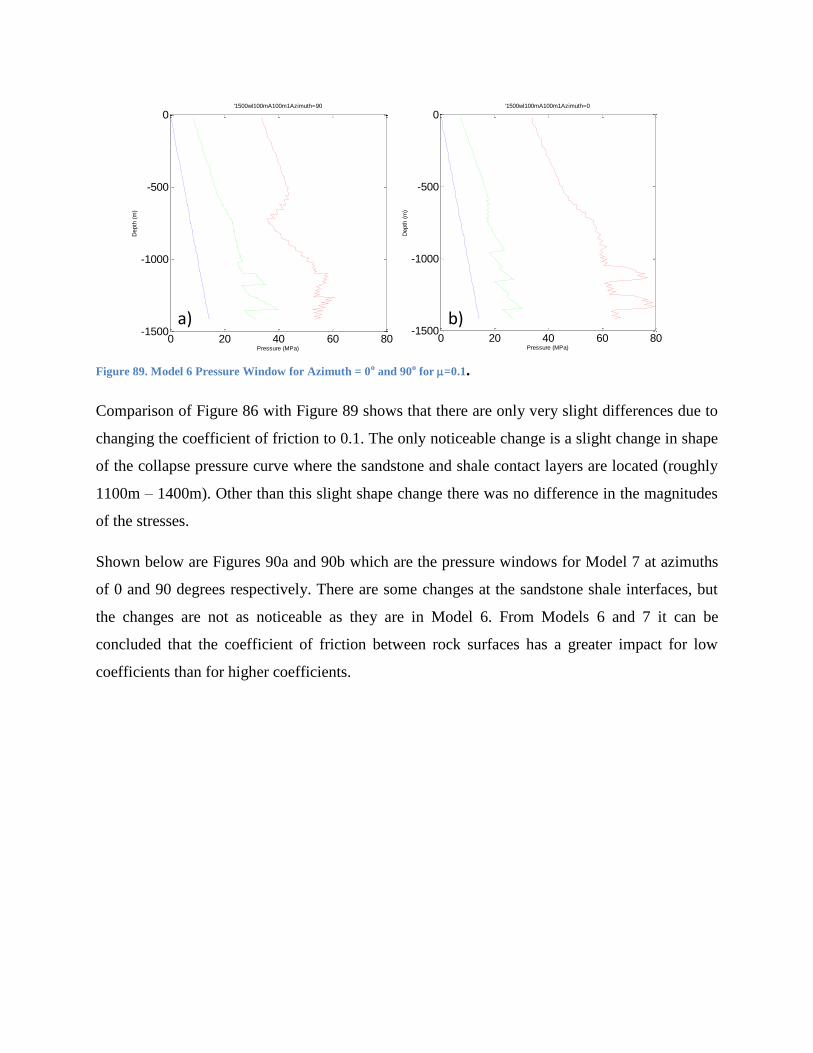
Figure 89. Model 6 Pressure Window for Azimuth = 0o and 90o for =0.1.
Comparison of Figure 86 with Figure 89 shows that there are only very slight differences due to
changing the coefficient of friction to 0.1. The only noticeable change is a slight change in shape
of the collapse pressure curve where the sandstone and shale contact layers are located (roughly
1100m – 1400m). Other than this slight shape change there was no difference in the magnitudes
of the stresses.
Shown below are Figures 90a and 90b which are the pressure windows for Model 7 at azimuths
of 0 and 90 degrees respectively. There are some changes at the sandstone shale interfaces, but
the changes are not as noticeable as they are in Model 6. From Models 6 and 7 it can be
concluded that the coefficient of friction between rock surfaces has a greater impact for low
coefficients than for higher coefficients.
0 20 40 60 80-1500
-1000
-500
0
Pressure (MPa)
Depth
(m
)
'1500wl100mA100m1Azimuth=90
0 20 40 60 80-1500
-1000
-500
0
Pressure (MPa)
Depth
(m
)
'1500wl100mA100m1Azimuth=0
a) b)

Figure 90. Model 7 Pressure Window for Azimuth = 0o and 90o.
2.2.8. Conclusions
The results for the wellbore stability analysis have shown that while vertical wells have proven
to be stable for all three stress regimes, a procedure has been developed that can be readily
applied to prospective case studies with more complex material models and geometries. The
procedure provides accurate results as proven by the validation model.
The procedure developed provides mud pressure window calculation for inclined wellbores of
type I wells. These wellbore types, especially type I wellbores with a horizontal hold section, are
relevant for CO2 sequestration applications, as horizontal wells have an increased surface area
inside the reservoir and thus feature increased injectivity. As predicted by Kirsch’s analytical
solution the in-situ stress regime has significant impact on stable drilling directions, whereby the
direction of the intermediate principal stress represents the least stable direction. This procedure
developed becomes of relevance when applied to case studies where the principal stresses are not
given by V, and h,H. In order to further improve the resulting wellbore stability analysis a
wellbore trajectory optimization procedure is necessary to account for scenarios where the
vertical stress is not a principal stress.
2.3.Wellbore Trajectory Optimization
2.3.1. Introduction
Wellbore trajectory planning plays an important role in the development and optimization of any
petroleum field. The placement of a wellbore may not only influence the amount of
0 20 40 60 80-1500
-1000
-500
0
Pressure (MPa)
Depth
(m
)
'1500wl100mA100m8Azimuth=0
0 20 40 60 80-1500
-1000
-500
0
Pressure (MPa)
Depth
(m
)
'1500wl100mA100m8Azimuth=90
a) b)

hydrocarbons contacted, but will also influence the ease at which a well is drilled [1, 2], its long-
term integrity [2] and affect hydraulic fracture stimulations [3]. With the advent of new drilling
techniques, the enhanced accuracy during the drilling process and the ability to drill various
types and shapes of wells has resulted in an demand and understanding of wellbore trajectory
planning [4, 5, 6]. Stable wellbore conditions with respect to mechanical failure are a function of
the geometrical trajectory within the 3D state of stress [1]. Wellbore stability can be predicted by
determining safe mud pressures preventing either borehole breakdown or collapse [1, 2, 4, 5, 6,
7, 8, 9]. Thus, a thorough knowledge of the in-situ stresses in the subsurface and how they
change during the life of a petroleum field is a crucial input parameter for planning stable
wellbores.
Most wellbore trajectory planning studies [1, 2, 3, 8, 9, 10, 11, 12, 13] assume an Andersonian
state of stress (ASoS) [14], where one principle stress is vertical; a common observation in the
Earth’s crust [7, 15]. Implicitly this assumption excludes many scenarios where complex
geologic conditions, such as heavily faulted or folded regions, areas subjected to salt dome
intrusion, and any shallow regions where unconsolidated rock is encountered, imply that the SoS
is not Andersionian and that shear stresses have to be considered [7, 10, 16]. When drilling in
regions where the stress tensor may be rapidly changing, an inclination or azimuth change of 5o
of the wellbore trajectory may result in a significant change in the stress magnitudes acting on
the wellbore wall. Assuming an ASoS also introduces a potentially misleading symmetry
between drilling directions. In an ASoS the conditions for the stable mud pressure window in any
azimuthal combination, which are 180o offset from each other, will be equal at the same
inclination. With the addition of shear stresses this is no longer true.
Another limitation of wellbore trajectory studies is the utilization of stereographic projections to
predict the safe mud pressure window [7, 13, 17, 18]. Stereographic projections enable
visualization of the full range of effects that inclination and azimuth have on the mud pressure
window. Unfortunately, these projection plots are only valid for a specific depth. Rapidly
changing stresses with depth could imply different conditions/orientations for a stable wellbore
and the overall stability of a wellbore trajectory cannot be studied in a continuous way.
In this paper we present a methodology for wellbore trajectory planning/optimization which
implements the complete stress tensor obtained from a numerical mechanical earth model

(MEM). This enables analysis of an arbitrary state of stress and precludes the simplification of
assuming an ASoS. Stereographic projections predicting stable wellbore orientations at certain
locations (starting at the target location in the reservoir) are used to find a suitable and stable
overall wellbore trajectory. The continuous stress data from the numerical model is extracted
along that planned well trajectory and the safe mud pressure window can be predicted for well
trajectories of different well types. The methodology described in this paper has been applied to
stresses extracted from a synthetic MEM of an offshore field in the Gulf of Mexico [GOM] and
best-fit wellbore trajectories and mud pressure windows are presented.
2.3.2. Theoretical Background
2.3.2.1.Stress in the Subsurface
At any point in the subsurface the state of stress is described by the stress tensor, σij, often
assumed to consist of the vertical and two horizontal principal stresses. This so called
Andersonian state of stress (ASoS) represents a common observation from stress measurements
in the Earth’s crust [7, 15]. If complex geologic conditions result in a non-ASoS the stress tensor
for effective stresses takes the form of:
(26)
Based on the stress tensor at any point the state of stress at a borehole of arbitrary orientation can
be calculated following equations 18-22 as presented above.
2.3.2.2.Failure Criteria and Safe Mud Pressure
In order to determine the safe mud pressure window, i.e. to determine collapse and breakdown
pressure, a combined Griffith-Mohr-Coulomb failure criterion is used. The procedure to
calculate breakdown and collapse pressures is described in detail by Lee et al. [21] and is exactly
followed here. Calculations of inclination/azimuthal wellbore stability (IAWBS) using
stereographic projections are used to calculate mud pressures (either breakdown or collapse) for
all combinations of azimuths and inclinations [13].
It should be noted that several studies have shown that the choice of the failure criterion used has
a significant influence on the prediction of the safe minimum mud pressures [22, 23, 24]. The
Mohr-Coulomb failure criterion is chosen for this study due to its simplicity and slightly more

conservative character for predicting the collapse pressure [7, 8]. However, the methodology for
wellbore trajectory planning presented in this paper can be applied using any failure criterion and
thus investigation of the impact of different failure criterions is beyond the scope of this paper.
For this study the rock properties required to calculate failure are assumed to be constant
throughout the volume. Cohesion, So, tensile strength, To, friction angle, ø, and Poisson’s ratio, ν
are given values of 10MPa, 5MPa, 30o, and 0.3 respectively. Clearly this is not the case in a real
world situation, where these parameters would change along the well trajectory, just as the
stresses are in these illustrative examples.
2.3.3. Application
3D numerical MEMs represent an excellent tool to simulate the state of stress in complex
geologic environments [25, 26, 27, 28]. When calibrated against existing stress measurements
numerical MEMs are capable of predicting realistic stress magnitudes and provide a continuous
3D data field of the state of stress. This stress field can then be used to determine the optimal
well path to a specific target location.
In the approach presented here, the 3D state of stress at a target location for a specific well path
is extracted from the numerical MEM and stereographic projections are used at each evaluation
location to determine the collapse pressure, Pc, the fracture gradient, Pbd, and the pressure
difference, Pdiff=Pbd-Pc, for all possible combinations of azimuths and inclinations. The optimal
angles for azimuth and inclination are determined by the largest pressure difference between
breakdown and collapse pressure. In other words, the full range of inclination/azimuthal mud
pressure windows is obtained at each location along the proposed well and then collapsed into a
single parameter (Pdiff) that can be optimized for. If the surface location of the drilling rig is fixed
(e.g. pad or template based drilling) the following procedure can be used to find optimal well
inclinations and KOP locations. If the surface location of the rig is flexible, the procedure can be
used to find both optimal drilling azimuths (i.e. surface location) and inclinations.
For the methodology presented here, all stereographic projections contain the Pdiff data calculated
for every combination of azimuth and inclination. The stereographic projections display each
data point on a polar plot with the azimuth being the angle around the circle (0o being North and
increasing toward the East), and inclinations plotted as concentric circles of varying radii.
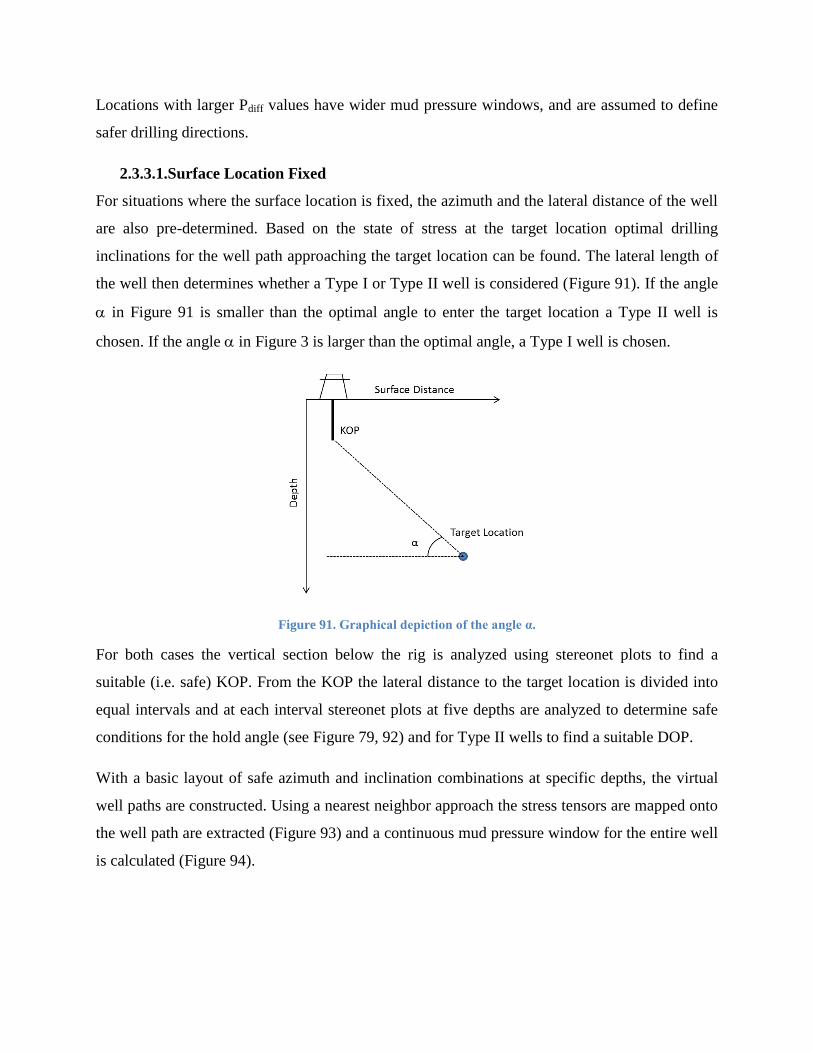
Locations with larger Pdiff values have wider mud pressure windows, and are assumed to define
safer drilling directions.
2.3.3.1.Surface Location Fixed
For situations where the surface location is fixed, the azimuth and the lateral distance of the well
are also pre-determined. Based on the state of stress at the target location optimal drilling
inclinations for the well path approaching the target location can be found. The lateral length of
the well then determines whether a Type I or Type II well is considered (Figure 91). If the angle
in Figure 91 is smaller than the optimal angle to enter the target location a Type II well is
chosen. If the angle in Figure 3 is larger than the optimal angle, a Type I well is chosen.
Figure 91. Graphical depiction of the angle α.
For both cases the vertical section below the rig is analyzed using stereonet plots to find a
suitable (i.e. safe) KOP. From the KOP the lateral distance to the target location is divided into
equal intervals and at each interval stereonet plots at five depths are analyzed to determine safe
conditions for the hold angle (see Figure 79, 92) and for Type II wells to find a suitable DOP.
With a basic layout of safe azimuth and inclination combinations at specific depths, the virtual
well paths are constructed. Using a nearest neighbor approach the stress tensors are mapped onto
the well path are extracted (Figure 93) and a continuous mud pressure window for the entire well
is calculated (Figure 94).
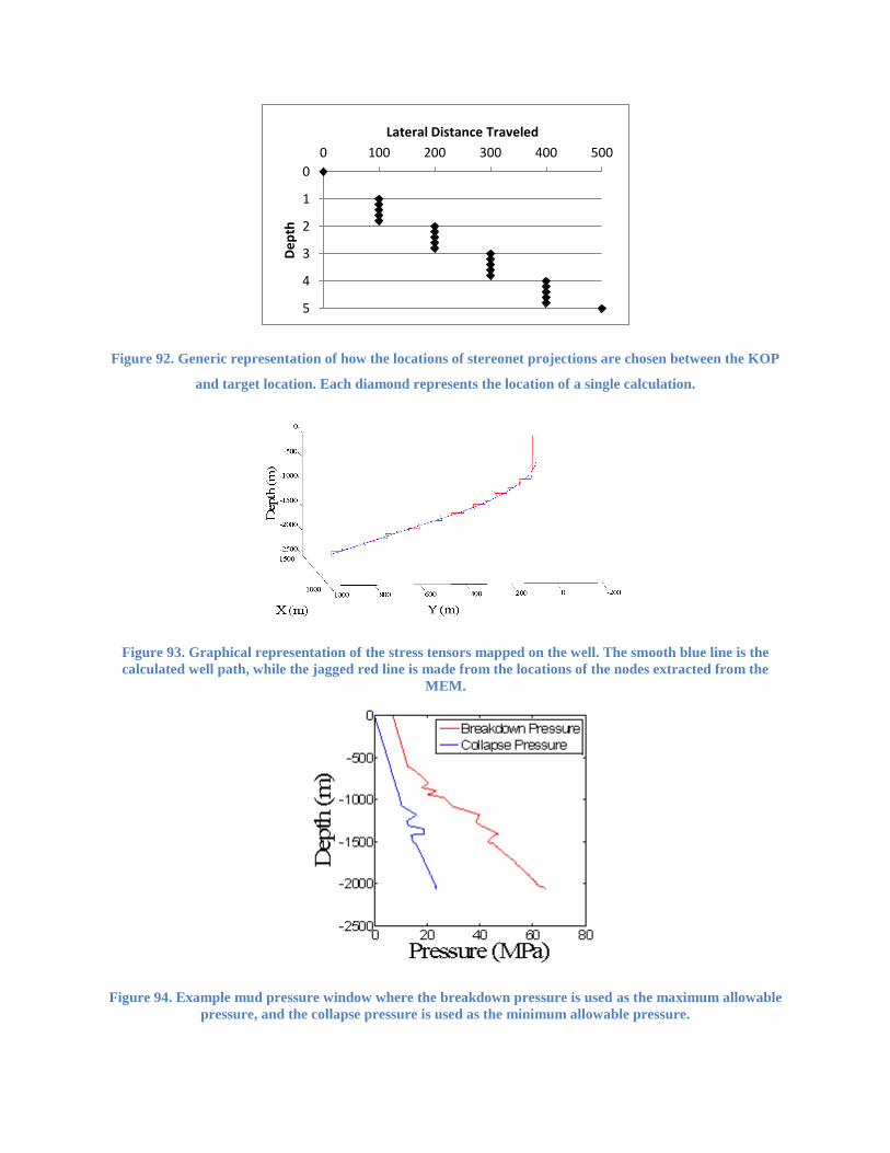
Figure 92. Generic representation of how the locations of stereonet projections are chosen between the KOP
and target location. Each diamond represents the location of a single calculation.
Figure 93. Graphical representation of the stress tensors mapped on the well. The smooth blue line is the
calculated well path, while the jagged red line is made from the locations of the nodes extracted from the
MEM.
Figure 94. Example mud pressure window where the breakdown pressure is used as the maximum allowable
pressure, and the collapse pressure is used as the minimum allowable pressure.
0
1
2
3
4
5
0 100 200 300 400 500
De
pth
Lateral Distance Traveled
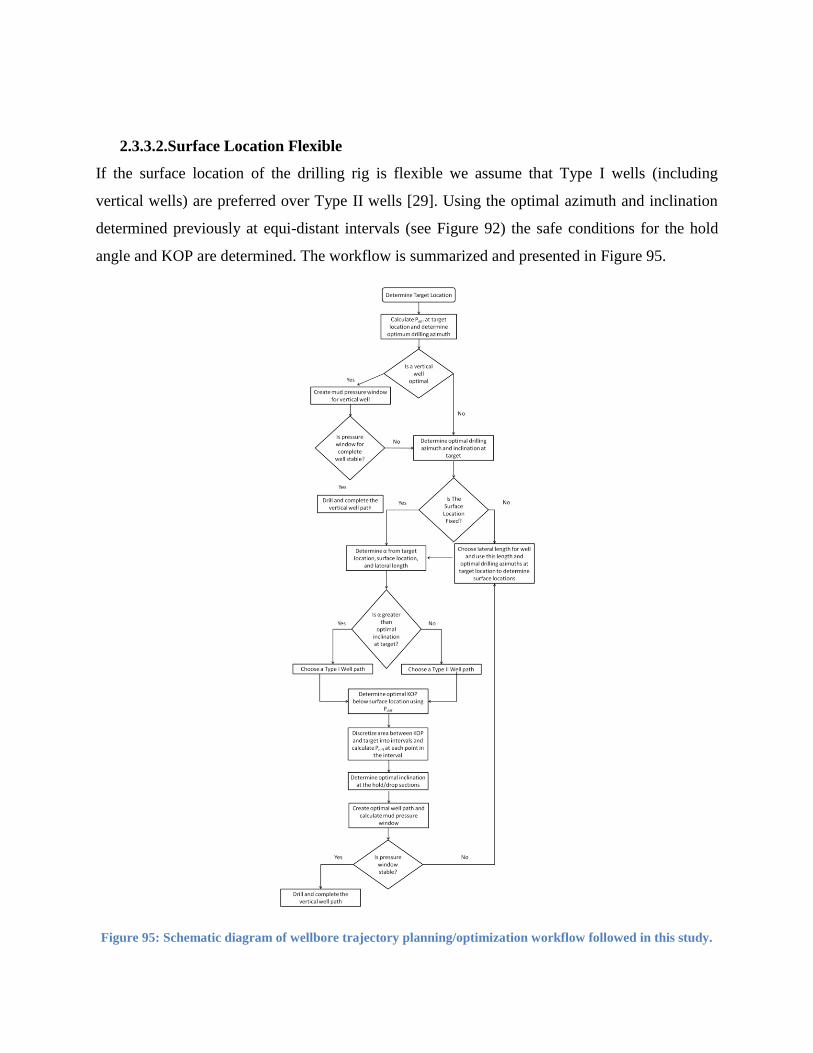
2.3.3.2.Surface Location Flexible
If the surface location of the drilling rig is flexible we assume that Type I wells (including
vertical wells) are preferred over Type II wells [29]. Using the optimal azimuth and inclination
determined previously at equi-distant intervals (see Figure 92) the safe conditions for the hold
angle and KOP are determined. The workflow is summarized and presented in Figure 95.
Figure 95: Schematic diagram of wellbore trajectory planning/optimization workflow followed in this study.
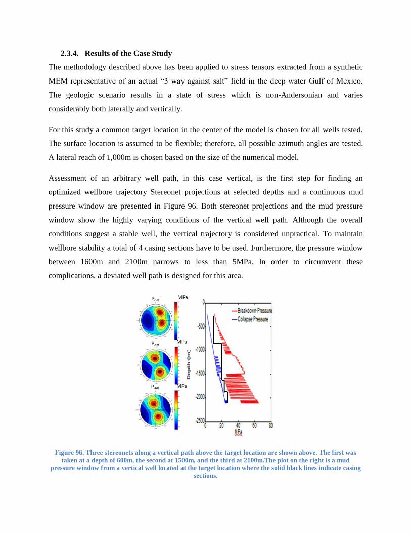
2.3.4. Results of the Case Study
The methodology described above has been applied to stress tensors extracted from a synthetic
MEM representative of an actual “3 way against salt” field in the deep water Gulf of Mexico.
The geologic scenario results in a state of stress which is non-Andersonian and varies
considerably both laterally and vertically.
For this study a common target location in the center of the model is chosen for all wells tested.
The surface location is assumed to be flexible; therefore, all possible azimuth angles are tested.
A lateral reach of 1,000m is chosen based on the size of the numerical model.
Assessment of an arbitrary well path, in this case vertical, is the first step for finding an
optimized wellbore trajectory Stereonet projections at selected depths and a continuous mud
pressure window are presented in Figure 96. Both stereonet projections and the mud pressure
window show the highly varying conditions of the vertical well path. Although the overall
conditions suggest a stable well, the vertical trajectory is considered unpractical. To maintain
wellbore stability a total of 4 casing sections have to be used. Furthermore, the pressure window
between 1600m and 2100m narrows to less than 5MPa. In order to circumvent these
complications, a deviated well path is designed for this area.
Figure 96. Three stereonets along a vertical path above the target location are shown above. The first was
taken at a depth of 600m, the second at 1500m, and the third at 2100m.The plot on the right is a mud
pressure window from a vertical well located at the target location where the solid black lines indicate casing
sections.
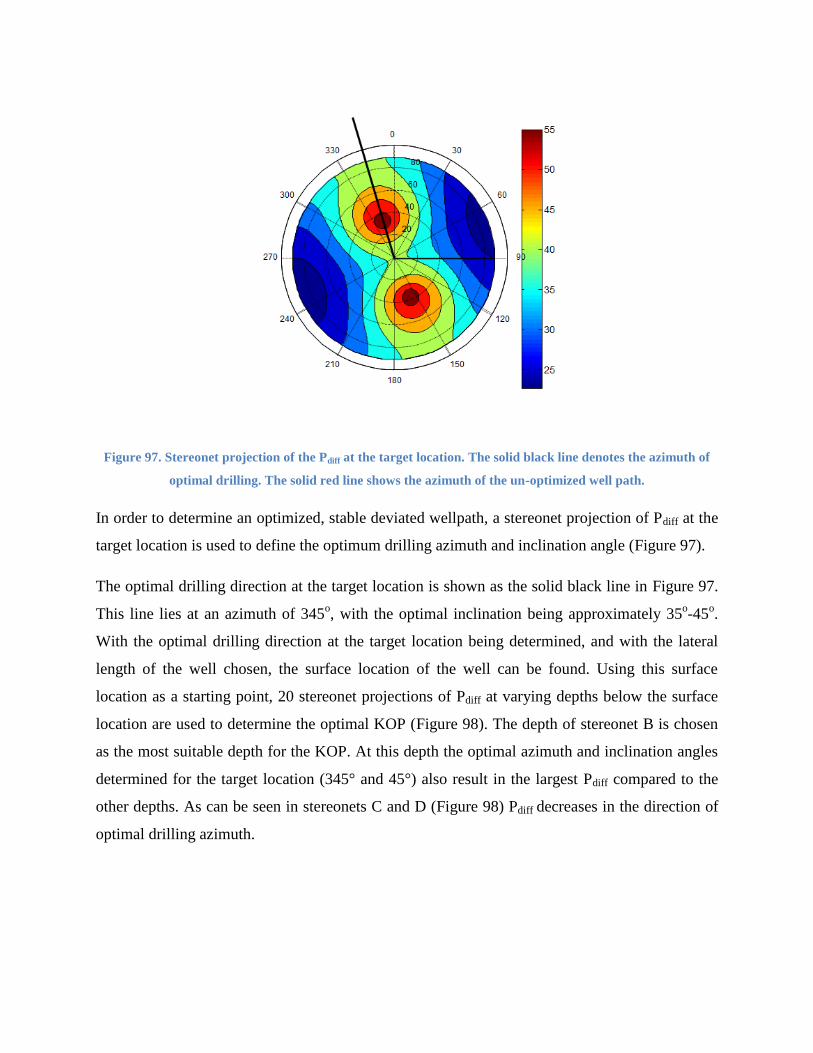
Figure 97. Stereonet projection of the Pdiff at the target location. The solid black line denotes the azimuth of
optimal drilling. The solid red line shows the azimuth of the un-optimized well path.
In order to determine an optimized, stable deviated wellpath, a stereonet projection of Pdiff at the
target location is used to define the optimum drilling azimuth and inclination angle (Figure 97).
The optimal drilling direction at the target location is shown as the solid black line in Figure 97.
This line lies at an azimuth of 345o, with the optimal inclination being approximately 35
o-45
o.
With the optimal drilling direction at the target location being determined, and with the lateral
length of the well chosen, the surface location of the well can be found. Using this surface
location as a starting point, 20 stereonet projections of Pdiff at varying depths below the surface
location are used to determine the optimal KOP (Figure 98). The depth of stereonet B is chosen
as the most suitable depth for the KOP. At this depth the optimal azimuth and inclination angles
determined for the target location (345° and 45°) also result in the largest Pdiff compared to the
other depths. As can be seen in stereonets C and D (Figure 98) Pdiff decreases in the direction of
optimal drilling azimuth.
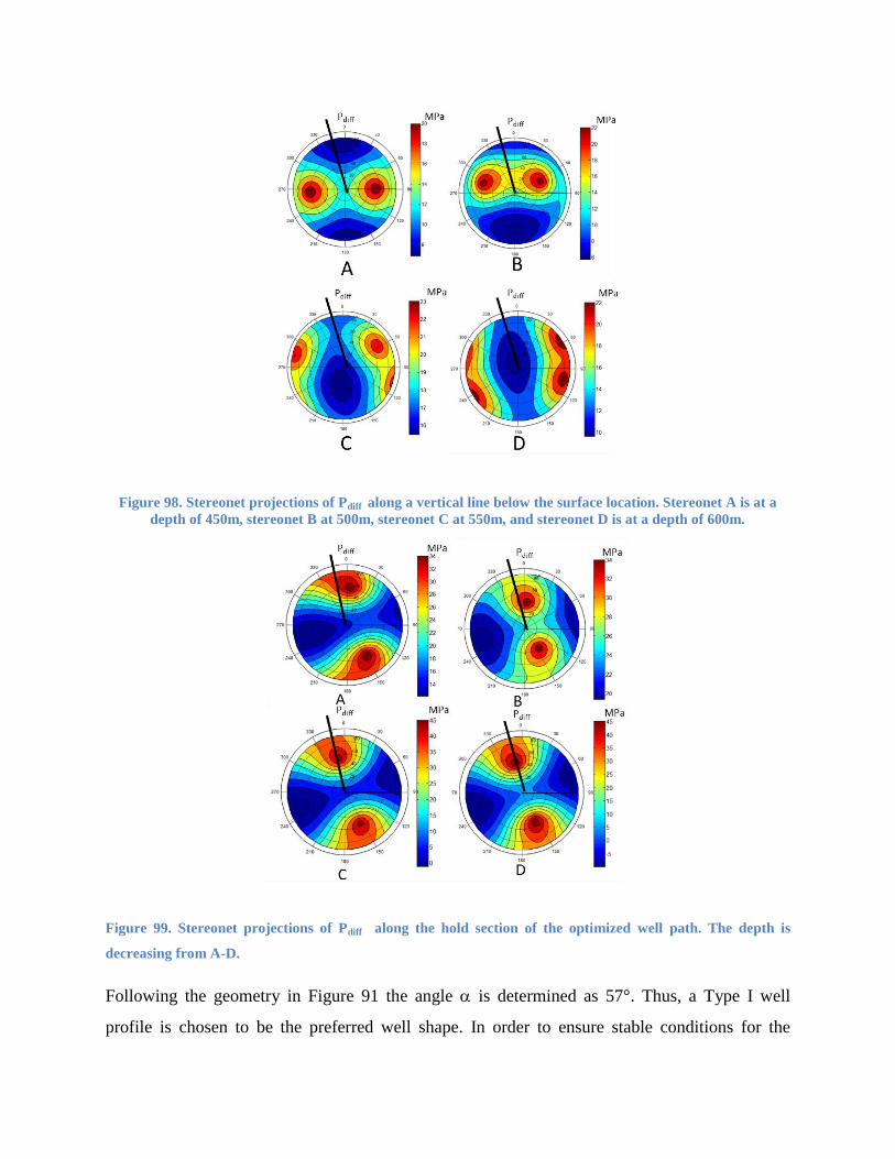
Figure 98. Stereonet projections of Pdiff along a vertical line below the surface location. Stereonet A is at a
depth of 450m, stereonet B at 500m, stereonet C at 550m, and stereonet D is at a depth of 600m.
Figure 99. Stereonet projections of Pdiff along the hold section of the optimized well path. The depth is
decreasing from A-D.
Following the geometry in Figure 91 the angle is determined as 57°. Thus, a Type I well
profile is chosen to be the preferred well shape. In order to ensure stable conditions for the
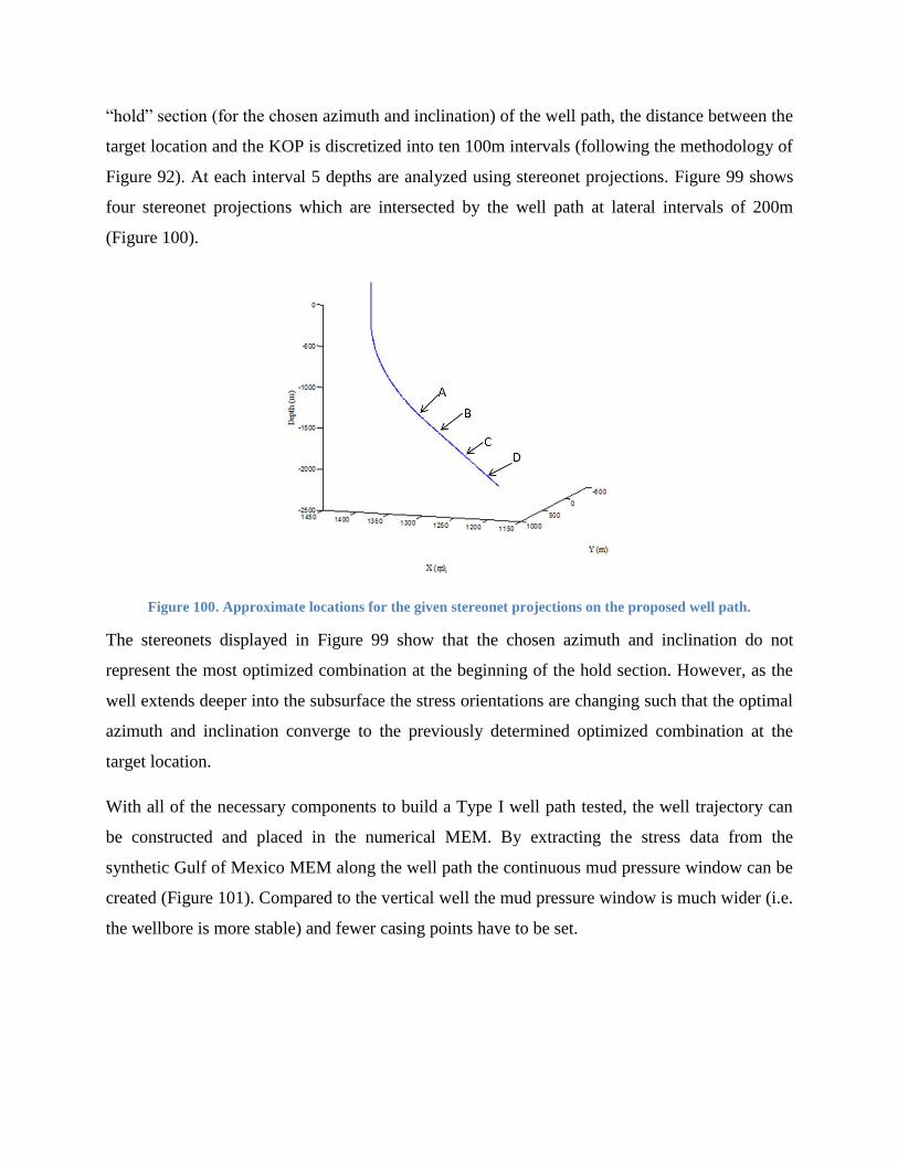
“hold” section (for the chosen azimuth and inclination) of the well path, the distance between the
target location and the KOP is discretized into ten 100m intervals (following the methodology of
Figure 92). At each interval 5 depths are analyzed using stereonet projections. Figure 99 shows
four stereonet projections which are intersected by the well path at lateral intervals of 200m
(Figure 100).
Figure 100. Approximate locations for the given stereonet projections on the proposed well path.
The stereonets displayed in Figure 99 show that the chosen azimuth and inclination do not
represent the most optimized combination at the beginning of the hold section. However, as the
well extends deeper into the subsurface the stress orientations are changing such that the optimal
azimuth and inclination converge to the previously determined optimized combination at the
target location.
With all of the necessary components to build a Type I well path tested, the well trajectory can
be constructed and placed in the numerical MEM. By extracting the stress data from the
synthetic Gulf of Mexico MEM along the well path the continuous mud pressure window can be
created (Figure 101). Compared to the vertical well the mud pressure window is much wider (i.e.
the wellbore is more stable) and fewer casing points have to be set.
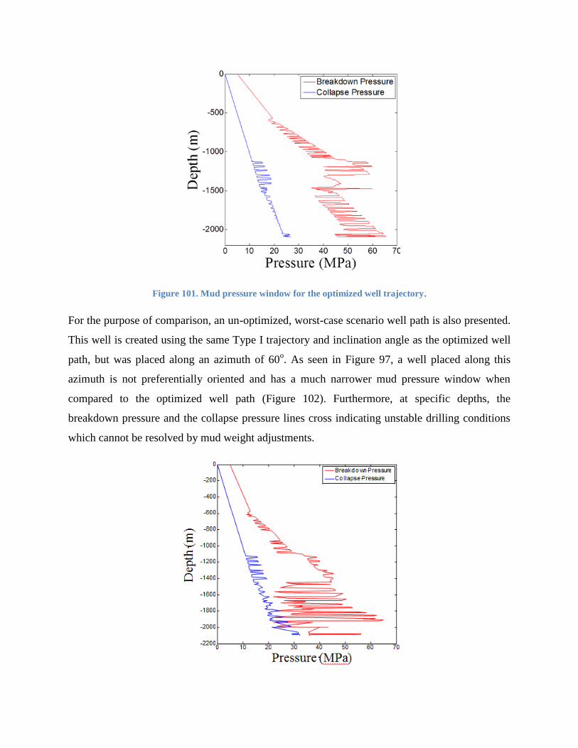
Figure 101. Mud pressure window for the optimized well trajectory.
For the purpose of comparison, an un-optimized, worst-case scenario well path is also presented.
This well is created using the same Type I trajectory and inclination angle as the optimized well
path, but was placed along an azimuth of 60o. As seen in Figure 97, a well placed along this
azimuth is not preferentially oriented and has a much narrower mud pressure window when
compared to the optimized well path (Figure 102). Furthermore, at specific depths, the
breakdown pressure and the collapse pressure lines cross indicating unstable drilling conditions
which cannot be resolved by mud weight adjustments.
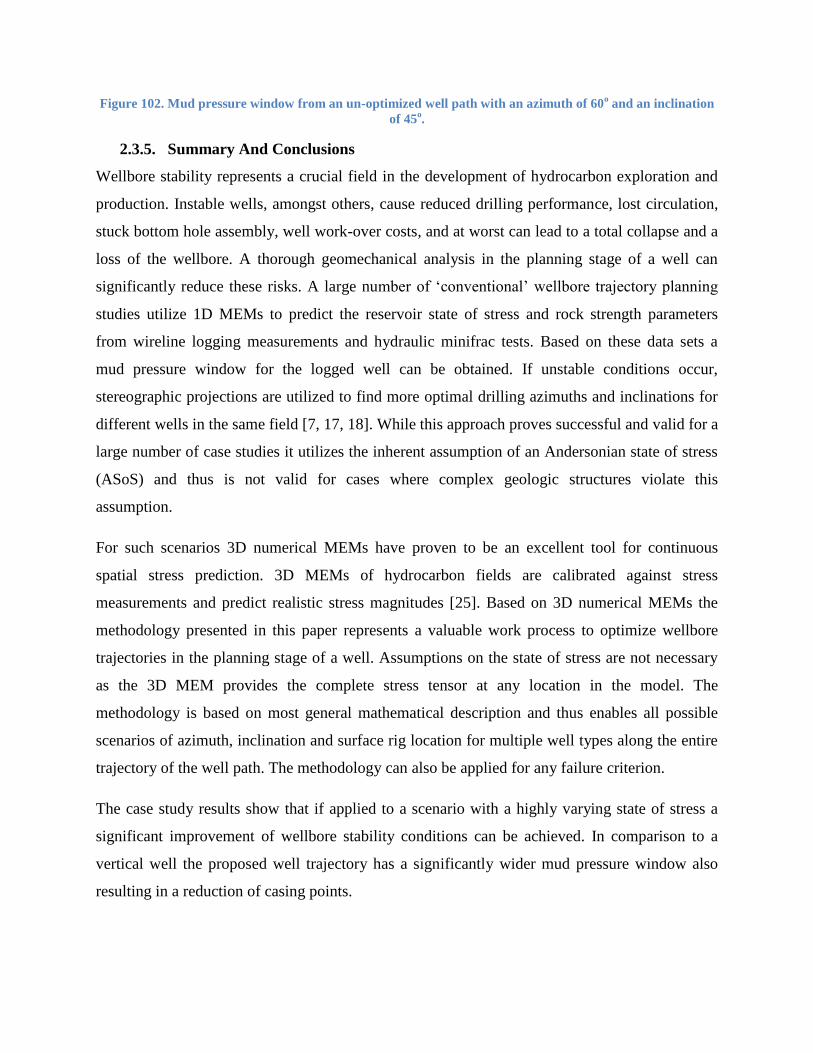
Figure 102. Mud pressure window from an un-optimized well path with an azimuth of 60o and an inclination
of 45o.
2.3.5. Summary And Conclusions
Wellbore stability represents a crucial field in the development of hydrocarbon exploration and
production. Instable wells, amongst others, cause reduced drilling performance, lost circulation,
stuck bottom hole assembly, well work-over costs, and at worst can lead to a total collapse and a
loss of the wellbore. A thorough geomechanical analysis in the planning stage of a well can
significantly reduce these risks. A large number of ‘conventional’ wellbore trajectory planning
studies utilize 1D MEMs to predict the reservoir state of stress and rock strength parameters
from wireline logging measurements and hydraulic minifrac tests. Based on these data sets a
mud pressure window for the logged well can be obtained. If unstable conditions occur,
stereographic projections are utilized to find more optimal drilling azimuths and inclinations for
different wells in the same field [7, 17, 18]. While this approach proves successful and valid for a
large number of case studies it utilizes the inherent assumption of an Andersonian state of stress
(ASoS) and thus is not valid for cases where complex geologic structures violate this
assumption.
For such scenarios 3D numerical MEMs have proven to be an excellent tool for continuous
spatial stress prediction. 3D MEMs of hydrocarbon fields are calibrated against stress
measurements and predict realistic stress magnitudes [25]. Based on 3D numerical MEMs the
methodology presented in this paper represents a valuable work process to optimize wellbore
trajectories in the planning stage of a well. Assumptions on the state of stress are not necessary
as the 3D MEM provides the complete stress tensor at any location in the model. The
methodology is based on most general mathematical description and thus enables all possible
scenarios of azimuth, inclination and surface rig location for multiple well types along the entire
trajectory of the well path. The methodology can also be applied for any failure criterion.
The case study results show that if applied to a scenario with a highly varying state of stress a
significant improvement of wellbore stability conditions can be achieved. In comparison to a
vertical well the proposed well trajectory has a significantly wider mud pressure window also
resulting in a reduction of casing points.

Although neither stereographic projections nor mud pressure windows alone can produce
optimal wellbore trajectory results, the combination of the two can be a powerful tool for
predicting optimal drilling directions. The presented methodology however, still utilizes
significant ‘human’ effort for analyzing stereonets at various locations of a deviated well path.
As the 3D MEM provides all necessary input data, the next step for the presented methodology is
to find an automatic process to find an optimal well trajectory for a given target location.
3. Overall Concluding Remarks and Accomplishments
In this ARRA training project 4 graduate students (3MS, 1PhD) have been employed and been
trained in numerical modeling of CO2 sequestration applications.
In contrast to the majority of numerical modeling studies for CO2 sequestration applications this
project does not employ horizontally layered basin models but focuses on a set of generic
anticline structures. Anticline structures are the most prominent structural trap for mature
hydrocarbon reservoirs and hence represent prime targets for CO2 sequestration sites. The
geometry of an anticline induces stress heterogeneities which in turn result in differences when
geomechanical risks such as fracture reactivation are analyzed. As a major conclusion, if
geometry information is available (i.e. 3D seismic), numerical models should not be simplified to
horizontally layered basins. The results of the pre-injection risk assessment on maximum
sustainable pore pressures based on finite element analysis and the results of the coupled fluid
flow – geomechanical analysis have shown that the prevailing stress regime is the most
important input parameter for geomechanical models. It is therefore recommended that every
geomechanical study utilized for CO2 sequestration case studies is calibrated by stress
measurements such as mini-frac tests.
Furthermore, these stress heterogeneities are emphasized when inter-bedding friction is
considered. This study has shown that low friction results in an effective mechanical decoupling
between adjacent beds and thus lower pore pressures can be sustained (i.e. for the compressional
stress regime).

If only fluid flow processes are considered the project results show that the fluid flow boundary
conditions are the most important parameter and huge differences are observed between open
and closed fluid systems. It is recommended that further research is conducted in order to
develop methods to quantify this crucial parameter.
On the borehole scale a methodology has been established to setup and optimize numerical
models in order to minimize errors. The results of the FE models on the reservoir scale have been
used to perform a wellbore stability analysis and to find stable drilling directions for the anticline
structures. While vertical wells have proven to be stable for all three stress regimes, a procedure
has been developed that can be readily applied to prospective case studies with more complex
material models and geometries. The procedure developed provides mud pressure window
calculation for inclined wellbores of type I wells. The methodology developed represents a
process to optimize wellbore trajectories in the planning stage of a well. Assumptions on the
state of stress are not necessary as the 3D FEM provides the complete stress tensor at any point
in the model. The methodology is based on the general mathematical description and thus
enables all possible scenarios of azimuth, inclination and surface rig location for multiple well
types along the entire trajectory of the well path. The case study results show that if applied to a
scenario with a highly varying state of stress a significant improvement of wellbore stability
conditions can be achieved.
As an overall conclusion the various numerical modeling techniques and analyses applied in this
project have shown that geometrical heterogeneities of the reservoir/injection layer have
significant influences on CO2 injection parameters. Whilst this project employed generic
anticline geometries and the results do not reflect an actual case study, the methodologies
developed in this project can be readily applied to any case study.
References
Aadnoy, B.S.. U. of Stavanger, and A.K. Hansen. 2005. Bounds on In-Situ Stress Magnitudes
Improve Wellbore Stability Analyses. SPE Journal. June: 115-120.
ABAQUS Analysis User’s Manual V6.10. Chapters 4.1.3 and 25.1.3. ABAQUS, Inc. Dassault
Systèmes.
Al-Ajmi, A.M., and R.W. Zimmerman. 2009. A new well path optimization model for increased
mechanical borehole stability. J. Pet. Sci. Eng. 69: 53-62.
Al-Ajmi, A.M., U. Sultan Qaboos, and R.W. Zimmerman. 2006. Stability Analysis of Deviated
Boreholes Using the Mogi-Coulomb Failure Criterion, With Applications to Some Oil and Gas
Reservoirs. In IADC/SPE Asia Pacific Drilling Technology Conference and Exhibition,
Bangkok, Thailand, 13-15 November 2006. SPE 104035-MS.
Altmann. J.B, Mueller, T.M., Mueller, BI.R., Tingay, M.R.P., and Heidbach, O., 2010.
Poroelastic contribution to the reservoir stress path. International Journal of Rock Mechanics &
Mining Sciences, 47, pages 1104-13.
Amirlatifi, A., Eckert, A., Nygaard, R. and B. Bai. 2011. Estimation of reservoir uplift,
seismicity and failure likelihood during CO2 injection through coupled reservoir simulation.
Paper CSUG/SPE 148946-PP presented in Canadian Unconventional Resources Conference,
Calgary, Canada, 15–17 November 2011.
Amirlatifi, A., Eckert, A., Nygaard, R. and B. Bai. 2011. Prediction of caprock fractures during
CO2 sequestration by coupled modeling in complex geological fields. In preceedings of tenth
annual conference on carbon capture and sequestration, Pittsburgh, USA, 2-5 May 2011.
Amirlatifi, A., Eckert, A., Nygaard, R., Bai, B., Liu, X., Paradeis, M., 2012. Role of Geometrical
Influences of CO2 Sequestration in Anticlines, in: 46th US Rock Mechanics / Geomechanics
American Rock Mechanics Assosiaction Symposium. Chicago, IL, p. ARMA 12–255.
Bachu, S., Gunter, W.D. and E.H. Perkins. 1994. Aquifer disposal of CO2: hydrodynamic and
mineral trapping. Energy Conversion and Management, 35 (4): 269-279.
Barton, C., M. D. Zoback, and D. Moos, 1995. Fluid flow along potentially active faults in
crystalline rock, Geology. 23: 683–686.
Barton, C.A. and Moos, D., Peska, P., and Zoback, M.D. 1997. Utilizing Wellbore Image Data to
Determine the Complete Stress Tensor: Application to Permeability Anisotropy and Wellbore
Stability. The Log Analyst. 38:6.
Biot, M. 1941. General Theory of Three Dimensional Consolidation. J. of Applied Physics.
12:155-164.
Birkholzer, J.T., Zhou, Q. and C.F. Tsang. 2009. Large-scale impact of CO2 storage in deep
saline aquifers: a sensivity study on pressure response in stratified systems. Int. J. of Greenhouse
Gas Control 3: 181-194
Bourgoyne, A.T. Jr., K.K. Millheim, M.E. Chenevert, and F.S. Young Jr. 1986. Applied Drilling
Engineering. Volume 2. SPE textbook series.
Bradley, W.B. 1979. Failure of inclined boreholes. J. Energy Resour. Technol. 101: 232-239.
Brudy, M., M.D. Zoback, K. Fuchs, F. Rummel, and J. Baumgärtner. 1997. Estimation of the
complete stress tensor to 8km depth in the KTB scientific drill holes: Implications for crustal
strength. J. of Geoph. Res. 102(B8): 18,453-18,475.
Buchman, T.J., G. Peters, and P.T. Connolly. 2008. Recent faulting in the Upper Rhine Graben
(Germany): a 3D finite element approach to predict fault reactivation. In 42nd
U.S. Rock
Mechanics Symposium and 2nd
U.S.-Canada Rock Mechanics Symposium, San Francisco, CA,
29 June – 2 July.
Byerlee, J. 1978. Friction of rocks. Pure and Applied Geophysics. 116: 615-626.
Cappa, F. and J. Rutqvist. 2011. Modeling of coupled deformation and permeability evolution
during fault reactivation induced by deep underground injection of CO2. Int. J. of Greenhouse
Gas Control. 5: 336-346.
Chen, G., M.E. Chenevert, M.M. Sharma, and M. Yu. 2003. A study of wellbore stability in
shales including poroelastic, chemical, and thermal effects. Journal of Petroleum Science and
Engineering. 38: 167-176.
Cheng, H., and M.B. Dusseault. 1993. Development and application of a fully-coupled two-
dimensional finite element approach to deformation and pressure diffusion around a borehole.
Journal of Canadian Petroleum Technology. 32: 28-38.
Cooper, G.A. 1994. Directional Drilling. Scientific American. 270(5): 82-87.
Coulomb, C.A. 1776. Essai sur une application des regles des maximis et minimis a quelquels
problemesde statique relatifs, a la architecture. Mem. Acad. Roy. Div. Sav. 7: 343-387.
Craupner, B. J., Li, D. and S. Bauer. 2011. The coupled simulator Eclipse-OopenGeoSys for the
simulation of CO2 storage in saline formations. J. Energy Procedia 4: 3794-3800
Dean. R.H., Gai, X., Stone, C.M. and S.E. Minkoff. 2006. A Comparison of Techniques for
Coupling Porous Flow and Geomechanics. SPE J. 11 (1):132-140.
Eckert, A., 2007: 3D multi-scale finite element analysis of the crustal state of stress in the
Western US and the Eastern California Shear Zone, and implications for stress – fluid flow
interactions for the Coso Geothermal Field. PhD thesis, Universitaet Karlsruhe.
Eckert, A., and P.T. Connolly. 2004. 2D Finite Element Modelling of Regional and Local
Fracture Networks in the Eastern California Shear Zone and Coso Range, California USA.
Geothermal Resources Council Transaction. 28: 643-648.
Ehlig-Economides, C. and M.J. Economides. 2010. Sequestering carbon dioxide in a
closedunderground volume. J. Pet. Sci. & Tech. 70: 123-130
Engelder T, Fischer MP. Influence of poroelastic behaviour on the magnitude of minimum
horizontal stress, Sh, in overpressured parts of sedimentary basins. Geology 1994,22:949–52.
Engelder, T. 1992. Stress Regimes in the Lithosphere. Princeton University Press.
9780691085555
Engelder, T., 1993. Stress Regimes in the Lithosphere. Princeton University Press.
Ewy, R.T. 1999. Wellbore-stability prediction by use of a modified Lade criterion. SPE Drilling
& Completion. 14: 85-91.
Feng, Y., and Shi, X. 2013. Hydraulic fracturing process: roles of in-situ stress and rock strength.
Adv. Mat. Res. 616-618: 435-440.
Fjaer, E., R.M. Holt, P. Horsrud, A.M. Raaen and R. Risnes. 1992. Petroleum Related Rock
Mechanics.. 2nd
ed. New York: Elsevier B.V.

Freitag, L., M. Jones, and P. Plassman. 1995. An Efficient Parallel Algorithm for Mesh
Smoothing. In Proceedings of the Fourth International Meshing Round Table, 1995, 47-58.
Gentzis, T., D. Nathan, and R.J. Chalaturnyk. 2009. A method to predict geomechanical
properties and model well stability in horizontal boreholes. International Journal of Coal. 78:
149-160.
Gibbs, J.F., Healy, J.H., Raleigh, C.B. & Coakley, J., 1973. Seismicity in the Rangely, Colorado,
area: 1962–1970, Bull. Seism. Soc. Am., 63, p. 1557–1570.
Goodman, H.E., and P. Connolly. 2007. Reconciling Subsurface Uncertainty With the
Appropriate Well Design Using the Mechanical Earth Model (MEM) Approach. In 31st Nigeria
Annual International Conference and Exhibition, Abuja, Nigeria, 6-8 August.
Grabinsky, M.W., R. Wilson, and A. Zougas. 1995. Practical meshing considerations for finite
element analysis of rock engineering problems. In 8th
ISRM Congress, Tokyo, Japan, 25-29
September 1995. SPE 8CONGRESS-1995-266.
Gray, K.E., E. Podnos, and E. Becker. 2009. Finite-Element Studies of Near-Wellbore Region
During Cementing Operations: Part I. SPE Drilling & Completion. 24: 127-136.
Hillis RR. Coupled changes in pore pressure and stress in oil fields and sedimentary basins. Pet
Geosci 2001;7:419–25.
Houseknecht, D.W. and F.G. Ethridge. 1978. Depositional history of the Lamotte sandstone of
southeastern Missouri. J. of Sedimentary Petrology 48 (2): 575-586.
http://www.sourcewatch.org/index.php?title=Existing_U.S._Coal_Plants, accessed January
2012.
Inoue, N. 2009. Answers to some questions about the coupling between fluid flow and rock
deformation in oil reservoirs. Paper SPE 125760 presented at SPE/EAGE Reservoir
Characterization and Simulation Conference, Abu Dhabi, UAE, 19- 21 October 2009.
Islam, M.A., Skalle, P., Al-Ajmi, A.M., and Søreide, O.K. 2010. Stability Analysis in Shale
through Deviated Boreholes using the Mohr and Mogi-Coulomb Failure Criteria. In 44th
US
Rock Mechanics Symposium and 5th
U.S.-Canada Rock Mechanics Symposium, Salt Lake City,
UT, 27-30 June.
Jaeger JC, Cook NGW, and Zimmerman RW. Fundamentals of Rock Mechanics. 4th edition,
Blackwell Publishin, Malden MA, USA, 2007.
Kirsch, G. 1898. Die Theorie der Elastizität und die Bedürfnisse der Festigkeitslehre. Zeitschrift
des Vereines Deutscher Ingenieure. 42: 797.
Knupp, P.M. 2000. Achieving finite Element Mesh Quality Via Optimization of the Jacobian
Matrix Norm and Associated Quantities. Part I- A Framework for Surface mesh Optimization.
Int. J. Numer. Meth. Engng. 48: 401-420.
Knupp, P.M. 2007. Remarks on mesh quality. In 45th
AIAA Aerospace Sciences Meeting and
Exhibit, Reno, NV, 7-10 January, 2007.
Kongsjorden, H., Karstad, O. and Tore A. Torp. 1998. Saline aquifer storage of carbon dioxide
in the Sleipner project. J. Waste Management 17 (5-6): 303-308
Last, N.C., and M.R. McLean. 1996. Assessing the Impact of Trajectory on Wells Drilled in an
Overthrust Region. JPT. July: 620-626.
Lee, M., A. Eckert, and R. Nygaard. 2011. Mesh optimization for finite element models of
wellbore stress analysis. In 45th
US Rock Mechanics/Geomechanics Symposium, San Francisco,
CA, 26-29 June.
Li, Q., Bai, Y., Yin, X., & Li, X. 2007. Thermo-hydro-mechanical modeling of CO2
sequestration system around fault environment. In Computational Earthquake Physics:
Simulations, Analysis and Infrastructure, Part II . 2585-2593. Birkhäuser Basel.
Li, Q., Z. Wu, and X. Li. 2009. Prediction of CO2 leakage during sequestration into marine
sedimentary strata. Energy Conservation and Management. 50:503-509.
Liu, X. 2011. Universal Technique Normalizes and Plans Various Well-Paths for Directional
Drilling. In SPE Middle East Oil and Gas Show and Conference, Manama, Bahrain, 25-28
September.
Loizzo, M., Lecampion, B., Bérard, T., Harichandran, A. and L. Jammes, 2009. Reusing O&G
Depleted Reservoirs for CO2 Storage: Pros and Cons. Paper SPE 124317-MS presented at SPE
Offshore Europe Oil & Gas Conference and Exhibition, Aberdeen, UK, 8-11 September 2009.
McLean, M.R., M.A. Addis. 1990. Wellbore stability: the effect of strength criteria on mud
weight recommendations. In SPE Annual Technical Conference and Exhibition, New Orleans,
LA, 23-26 September 1990. SPE 20405-MS.
Metz, B., O. Davidson, Bosch. P, Dave. R and L. A.Meyer (eds.). IPCC, 2007: Climate Change
2007: Mitigation of Climate Change. Contribution of Working Group III to the Fourth
Assessment Report of the Intergovernmental Panel on Climate Change. Cambridge University
Press, Cambridge, United Kingdom and New York, NY, USA.
Metz, B., O. Davidson, H. de Connick, M . Loos, and L. Meyer. 2005. IPCC Special report on
carbon dioxide capture and storage. Cambridge University Press.
Mitchell, S.A. 1997. Choosing corners of rectangles for mapped meshing. In Proceedings of the
thirteenth annual symposium on Computational geometry, New York, NY, 1997. 87-93.
Muller B, Altmann JB, M ¨ uller TM, Weisshardt A, Shapiro SA, Schilling F, Heidbach O.
Tensor character of pore pressure-stress coupling in reservoir depletion and injection. 72nd
EAGE Conference, Barcelona, 2010. Extended abstracts F045.
Nawrocki, P.A. 2010. Critical wellbore pressures using different rock failure criteria. In
International Symposium - 6th
Asian Rock Mechanics Symposium, New Delhi, India, 23-27
October 2010.
Nicholson, C., E. Roeloffs, and R. L. Wesson. 1986. The northeastern Ohio earthquake of 31
January 1986: was it induced? Seismological Society of America.
Nipp, H.-K, E.G. McNulty. 1987. Effects of mesh size and boundary conditions on creep
analysis of rock salt. In The 28th U.S. Symposium on Rock Mechanics, Tucsan, AZ, 29 June - 1
July 1987.
Paradeis, M., Eckert, A. and X. Liu. 2012. Influences of Anticline Reservoir Geometry on
Critical Pore Pressures Associated with CO2 Sequestration. Paper ARMA 12-319, to be
presented in 46th US Rock Mechanics Geomechanics Symposium, Chicago, USA, 24-27 June
2012.
Peska, P., and M.D. Zoback. 1995. Compressive and tensile failure of inclined well bores and
determination of in situ stress and rock strength. J. of Geo. Res. 100(B7): 12,791-12,811.
Pettersen, O. 2006. A predictor for accelerated coupled rock mechanics and reservoir simulation.
In proceedings of 10th European Conference on the Mathematics of Oil Recovery, Amsterdam,
Netherlands, 4-7 September 2006.
Pollar, D.D. and R.C. Flectcher. 2005. Fundamentals of Structural Geology. Cambridge
University Press.
R. J. Gibbs. 1973. Mechanisms of Trace Metal Transport in Rivers. Science. 180: 71-73 .
Rahim, Z., A.A. Al-Kanaan, H.A. Al-Anazi, and M.S. Ahmed. 2012. Successful drilling of
lateral wells in minimum horizontal stress direction for optimal fracture placement. Oil & Gas J.
110(12): 74-82.
Rutqvist, J. and C-F. Tsang, 2002. “A study of caprock hydromechanical changes associated
with CO2-injection into a brine formation.” Environmental Geology, 42, 296-305.
Rutqvist, J., J. Birkholzer, and C.-F. Tsang. 2006. Modeling of geomechanical processes during
injection in a multilayered reservoir-caprock system and implications on site characterization. In
Proceedings of the International Symposium on Site Characterization for CO2 Geological
Storage, Berkeley, 20-22 March 2006.
Ruqvist, J., Birkholzer, J., Cappa, F. and C.F. Tsang. 2007. Estimating maximum sustainable
injection pressure during geological sequestration of CO2 using coupled fluid flow and
geomechanical fault-slip analysis. J. of Energery Conversion and Management 48: 1798-1807
Rutqvist, J., J. Birkholzer, and C.-F. Tsang. 2008. Coupled reservoir-geomechanical analysis of
the potential for tensile and shear failure associated with CO2 injection in multilayered reservoir-
caprock systems. Int. J. of Rock Mechanics and Mining Sciences. 45: 132-143.
Rutqvist, J. and F. Cappa. 2011. Modeling of coupled deformation and permeability evolution
during fault reactivation induced by deep underground injection of CO2. Int. J. of Greenhouse
Gas Control. 5: 336-346.
Rutqvist, J., P. Digby, and O. Stephansson. 1989. Simulation of borehole breakouts with a
damage material model. In ISRM International Symposium, Pau, France, 30 August - 2
September 1989.
Samier, P. and S.D. Gennaro. 2007. Pratical iterative coupling of geomechanics with reservoir
simulation. Paper SPE 106188, presented at SPE Reservoir Simulation Symposium, Houston,
USA,26-28 February 2007.
Sanz, P.F., Pollard, D.D., Allwardt, P.F., and Borja, R.I., 2008. Mechanical models of fracture
reactivation and slip on bedding surfaces during folding of the asymmetric anticline at Sheep
Mountain, Wyoming. Journal of Structural Geology, vol. 30, no. 9, pp. 1177-1191.
Schutjens, P.M.T.M., J.R. Snippe, H. Mahani, J. Turner, J. Ita, and A.P. Mossop. 2012.
Production-Induced Stress Change in and Above a Reservoir Pierced by Two Salt Domes: A
Geomechanical Model and Its Applications. SPE Journal. March: 80-97.
Settari, A. and F.M. Mourits, 1998. A coupled reservoir and geomechanical simulation system.
Paper SPE 50939. SPE J. 3 (3): 219-226.
Settari, A., and Walters, D. 2001. Advances in coupled geomechanical and reservoir modeling
with applications to reservoir compaction. Spe Journal, 6(3), 334-342..
Sibson, R.H., 2003. Brittle failure controls on maximum sustainable over-pressure in different
tectonic stress regimes. Bulletin American Society of Petroleum Geology, v.87, p. 901-908.
Smart, K. J., Ferrill, D. a., & Morris, A. P. 2009. Impact of interlayer slip on fracture prediction
from geomechanical models of fault-related folds. AAPG Bulletin, 93(11), 1447–1458.
Streit, J. and R. Hillis. 2004. Estimating fault stability and sustainable fluid pressure for
underground storage of CO2 in porous rock. Energy. 29: 1445-1456.
Taberner. C., Cartwright, L. and T. Xu. 2009. Injection of supercritical CO2 into deep saline
carbonate formations, predictions from geochemical modling. Paper SPE 121272 presented at
SPE EUROPEC/EAGE Annual Conference and Exhibition, Amsterdam, Netherlands, 8-11 June
2009.
Tan, Q., J. Deng, and B. Yu. 2013. Study on Borehole Stability of Unconsolidated Sandstone in
Depleted Reservoir. Adv. Mat. Res. 616-618: 720-725.
Teufel, L.W., Rhett, D.W., and Farrell, H.E., 1991. Effect of reservoir depletion and pore
pressure drawdown on in situ stress and deformation in the Ekofisk Field, North Sea. In:
Roegiers, Editor, Rock Mechanics as a Multidisciplinary Science, Balkema Rotterdam, ISBN
906191194X, p. 63-72.
Thomas, L.K., Chin, L.Y., Pierson, R.G. and J.E. Sylte. 2003. Coupled Geomechanics and
Reservoir Simulation. SPE J. 8 (4): 350-358.
Tran, D. Shrivastava, V. Nghiem, L. and B. Kohs. 2009. Geomechanical risk mitigation for CO2
sequestration in saline aquifers. Paper SPE 125167 presented in SPE Annual Technical
Conference and Exhibition, New Orleans, USA, 4-7 October 2009.
Tran, D., Nghiem, L., Shrivastava, V., Kohse, B., 2010. Study of geomechanical effects in deep
aquifer CO2 storage, in: 44th US Rock Mechanics Symposium. ARMA, Salt Lake City, UT.
Tran, M. H., and Y.N. Abousleiman. 2010. The impacts of failure criteria and geological stress
states on the sensitivity of parameters in wellbore stability analysis. In 44th U.S. Rock
Mechanics Symposium and 5th U.S.-Canada Rock Mechanics Symposium, Salt Lake City, UT,
June 27 - 30, 2010.
Turon, A., C.G. Davila, P.P. Camanho, and J. Costa. 2007. An engineering solution for mesh
size effects in the simulation of delamination using cohesive zone models. Journal of
Engineering Fracture Mechanics. 74, 1665-1682.
Twiss, R.J., and Moores, E.M., 1992. Structural Geology.Freeman and Company, New York.
Twiss, R.J and E.M. Moores. 2007. Mechanics of Natural Fractures and Faults. In Structural
Geology, 2nd
ed. New York: W.H. Freeman and Company, 231-264.
Van der Meer, L. G. H. and J. D. van Wees. 2006.Limitations to Storage Pressure in Finite
Saline Aquifers and the Effects of CO2 Solubility on Storage Pressure. Paper SPE 103342
presented at the SPE Annual Technical Conference and Exhibition, San Antonio, Texas, 24-27
September.
Verdon, J.P, J.M. Kendall, D.J. White, and D.A. Angus. 2011. Linking microseismic event
observations with geomechanical models to minimize the risks of storing CO2 in geological
formations. Earth and Planetary Science Letters. 305: 143-152.
Vidal-Gilbert, S., J.-F.Nauroy, and E. Brosse, 2008. 3D geomechanical modeling for CO2
geologic storage in the Dogger carbonates of the Paris Basin. Int. J. Greenhouse Gas Control,
V.3, Issue 3, p. 288-299.
Wesson, R.L. and C. Nicholson. 1987. Earthquake Hazard Associated with Deep Well
Injection. Prepared by the U.S. Geological Survey. Open-File Report 87-331.

Wiprut, D. and M.D. Zoback. Constraining the full stress tensor in the Visund field, Norwegian
North Sea: Application to wellbore stability and sand production. Int'l. J. Rock Mech. & Mining
Sci., v. 37, pp. 317-336, 2000.
Yamamato, K., M. Tamura, N. Goto. 2006. Borehole instability analysis in an anisotropic and
heterogeneous shale formation. In IADC/SPE Asia Pacific Drilling Technology Conference and
Exhibition, Bangkok, Thailand, 13-15 November 2006. SPE 103883-MS.
Yang, X., L. Zhiyuan, H. Zhang, Q. Xiong, and H. Liu. 2012. An analysis on wellbore collapse
of open hold completion in carbonate formation. Appl. Mech. And Met. 220-223: 150-156.
Zahn, M.N., L.C. Coelho, L. Landau, and J.L.D. Alves. 2010. Numerical study on wellbore
stability analysis consindering volumetric failure. Mecánic Computacional. 29: 8837-8858.
Zare-Reisabadi, M.R., A. Kaffash, and S.R. Shadizadeh. 2012. Determination of optimal well
trajectory during drilling and production based on borehole stability. J. of Rock Mech. And Min.
Sci. 56: 77-87.
Zavattieri, P. 1996. Optimization Strategies in Unstructured Mesh Generation. International
Journal for Numerical Methods in Engineering. 39: 2055-2071.
Zervos, A., P. Papanastasiou, and J. Cook. 1998. Elastoplastic finite element analysis of inclined
wellbores. In SPE/ISRM Rock Mechanics in Petroleum Engineering, Trondheim, Norway. 8 - 10
July 1998. SPE/ISRM 47322.
Zhang, J., M. Bai, and J.-C. Roegiers. 2003. Dual-porosity poroelastic analyses of wellbore
stability. International Journal of Rock Mechanics and Mining Sciences. 40: 473-483.
Zhang, J., W.B. Standifird, K. Adesina, and G. Keaney. 2006. Wellbore stability with
consideration of pore pressure and drilling fluid interactions. In the 41st U.S. Symposium on
Rock Mechanics, Golden, CO, 17 - 21 June, 2006.
Zhang, L., P. Cao, and K.C. Radha. 2010. Evaluation of rock strength criteria for wellbore
stability analysis. International Journal of Rock Mechanics and Mining Sciences. 47: 1304-1316.
Zhou, Q., Birkholzer, J. T., Tsang, C.F. and J. Rutqvist. 2008. A method for quick assessment of
CO2 storage capacity in closed and semi-closed saline formations. Int. J. of Greenhouse Gas
Control 2: 626-639.

Zienkiewicz, O.C., R.L. Taylor, and J.Z. Zhu. The finite element method: its basis and
fundamentals. 6th ed. Butterworth-Heinemann.
Zoback, MD. Reservoir Geomechanics. Cambridge University Press, New York, 2007.
Zweigel, P. and L. Heill. 2003. Studies on the likelihood for caprock fracturing in the Sleipner
CO2 injection case. In Saline Aquifer CO2 Storage Project.
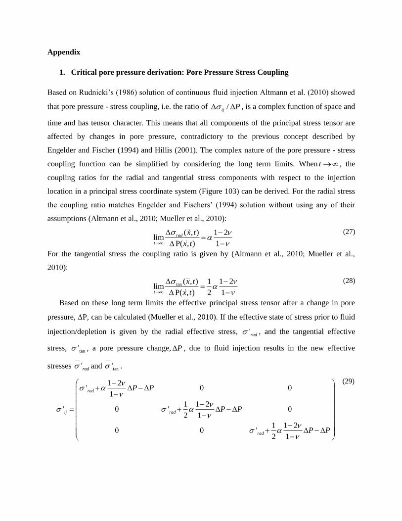
Appendix
1. Critical pore pressure derivation: Pore Pressure Stress Coupling
Based on Rudnicki’s (1986) solution of continuous fluid injection Altmann et al. (2010) showed
that pore pressure - stress coupling, i.e. the ratio of /ij P , is a complex function of space and
time and has tensor character. This means that all components of the principal stress tensor are
affected by changes in pore pressure, contradictory to the previous concept described by
Engelder and Fischer (1994) and Hillis (2001). The complex nature of the pore pressure - stress
coupling function can be simplified by considering the long term limits. When t , the
coupling ratios for the radial and tangential stress components with respect to the injection
location in a principal stress coordinate system (Figure 103) can be derived. For the radial stress
the coupling ratio matches Engelder and Fischers’ (1994) solution without using any of their
assumptions (Altmann et al., 2010; Mueller et al., 2010):
( , ) 1 2lim
P( , ) 1
rad
t
x t
x t
(27)
For the tangential stress the coupling ratio is given by (Altmann et al., 2010; Mueller et al.,
2010):
tan ( , ) 1 1 2
limP( , ) 2 1t
x t
x t
(28)
Based on these long term limits the effective principal stress tensor after a change in pore
pressure, P, can be calculated (Mueller et al., 2010). If the effective state of stress prior to fluid
injection/depletion is given by the radial effective stress, 'rad , and the tangential effective
stress, tan' , a pore pressure change, P , due to fluid injection results in the new effective
stresses 'rad and tan' .
1 2' 0 0
1
1 1 2' 0 ' 0
2 1
1 1 20 0 '
2 1
rad
ij rad
rad
P P
P P
P P
(29)
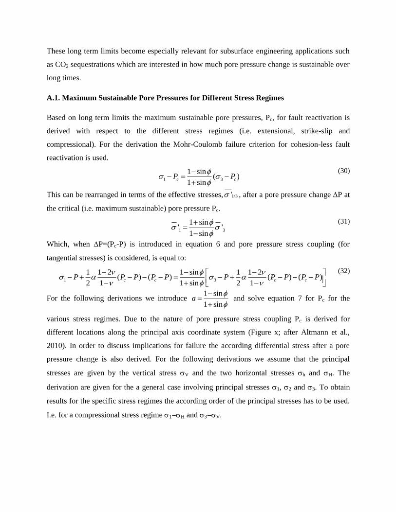
These long term limits become especially relevant for subsurface engineering applications such
as CO2 sequestrations which are interested in how much pore pressure change is sustainable over
long times.
A.1. Maximum Sustainable Pore Pressures for Different Stress Regimes
Based on long term limits the maximum sustainable pore pressures, Pc, for fault reactivation is
derived with respect to the different stress regimes (i.e. extensional, strike-slip and
compressional). For the derivation the Mohr-Coulomb failure criterion for cohesion-less fault
reactivation is used.
1 3
1 sin( )
1 sinc cP P
(30)
This can be rearranged in terms of the effective stresses, 1/3' , after a pore pressure change P at
the critical (i.e. maximum sustainable) pore pressure Pc.
1 3
1 sin' '
1 sin
(31)
Which, when P=(Pc-P) is introduced in equation 6 and pore pressure stress coupling (for
tangential stresses) is considered, is equal to:
1 3
1 1 2 1 sin 1 1 2( ) ( ) ( ) ( )
2 1 1 sin 2 1c c c cP P P P P P P P P P
(32)
For the following derivations we introduce 1 sin
1 sina
and solve equation 7 for Pc for the
various stress regimes. Due to the nature of pore pressure stress coupling Pc is derived for
different locations along the principal axis coordinate system (Figure x; after Altmann et al.,
2010). In order to discuss implications for failure the according differential stress after a pore
pressure change is also derived. For the following derivations we assume that the principal
stresses are given by the vertical stress V and the two horizontal stresses h and H. The
derivation are given for the a general case involving principal stresses 1, 2 and 3. To obtain
results for the specific stress regimes the according order of the principal stresses has to be used.
I.e. for a compressional stress regime 1=H and 3=V.
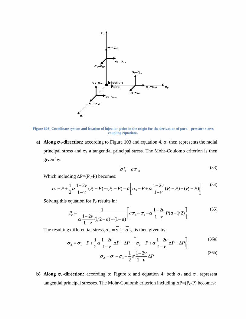
Figure 603: Coordinate system and location of injection point in the origin for the derivation of pore – pressure stress
coupling equations.
a) Along 3-direction: according to Figure 103 and equation 4, 3 then represents the radial
principal stress and 1 a tangential principal stress. The Mohr-Coulomb criterion is then
given by:
1 3' 'a (33)
Which including P=(Pc-P) becomes:
1 3
1 1 2 1 2( ) ( ) ( ) ( )
2 1 1c c c cP P P P P a P P P P P
(34)
Solving this equation for Pc results in:
3 1
1 1 2( 1 2)
1 2 1(1 2 ) (1 )
1
cP a P a
a a
(35)
The resulting differential stress, 1 3' 'd , is then given by:
1 3
1 1 2 1 2
2 1 1d P P P P P P
(36a)
1 3
1 1 2
2 1d P
(36b)
b) Along 2-direction: according to Figure x and equation 4, both 1 and 3 represent
tangential principal stresses. The Mohr-Coulomb criterion including P=(Pc-P) becomes:
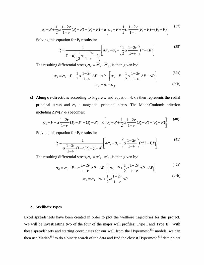
1 3
1 1 2 1 1 2( ) ( ) ( ) ( )
2 1 2 1c c c cP P P P P a P P P P P
(37)
Solving this equation for Pc results in:
3 1
1 1 1 2( 1)
1 1 2 2 1(1 ) 1
2 1
cP a a P
a
(38)
The resulting differential stress, 1 3' 'd , is then given by:
1 3
1 1 2 1 1 2
2 1 2 1d P P P P P P
(39a)
1 3d (39b)
c) Along1-direction: according to Figure x and equation 4, 1 then represents the radial
principal stress and 3 a tangential principal stress. The Mohr-Coulomb criterion
including P=(Pc-P) becomes:
1 3
1 2 1 1 2( ) ( ) ( ) ( )
1 2 1c c c cP P P P P a P P P P P
(40)
Solving this equation for Pc results in:
3 1
1 1 2( 2 1)
1 2 1(1 2) (1 )
1
cP a a P
a a
(41)
The resulting differential stress, 1 3' 'd , is then given by:
1 3
1 2 1 1 2
1 2 1d P P P P P P
(42a)
1 3
1 1 2
2 1d P
(42b)
2. Wellbore types
Excel spreadsheets have been created in order to plot the wellbore trajectories for this project.
We will be investigating two of the four of the major well profiles; Type I and Type II. With
these spreadsheets and starting coordinates for our well from the HypermeshTM
models, we can
then use MatlabTM
to do a binary search of the data and find the closest HypermeshTM
data points
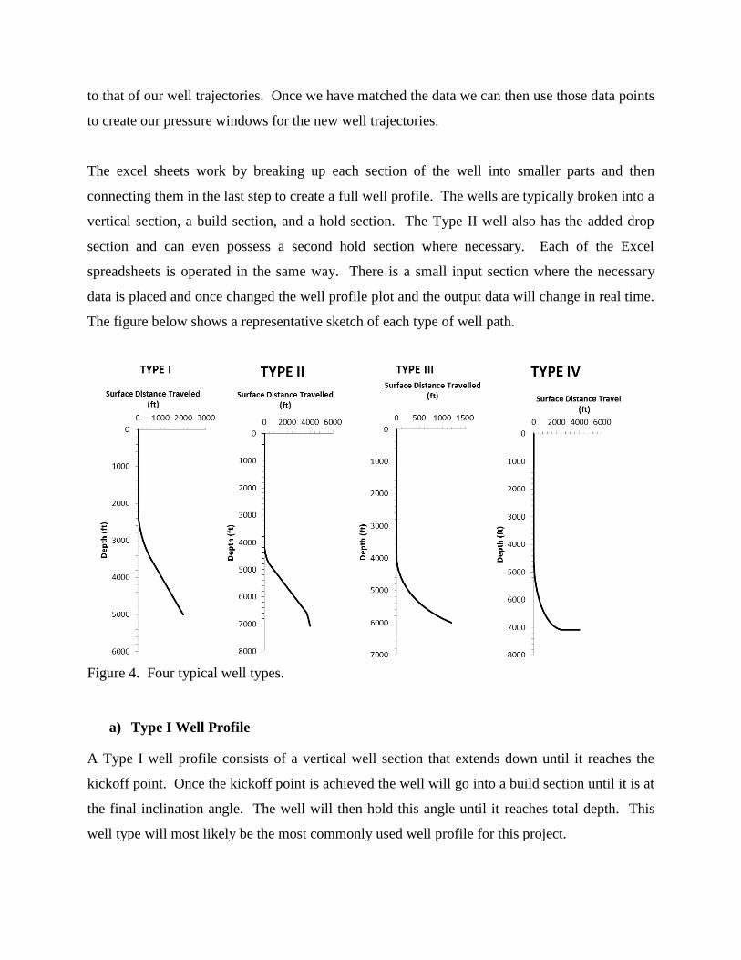
to that of our well trajectories. Once we have matched the data we can then use those data points
to create our pressure windows for the new well trajectories.
The excel sheets work by breaking up each section of the well into smaller parts and then
connecting them in the last step to create a full well profile. The wells are typically broken into a
vertical section, a build section, and a hold section. The Type II well also has the added drop
section and can even possess a second hold section where necessary. Each of the Excel
spreadsheets is operated in the same way. There is a small input section where the necessary
data is placed and once changed the well profile plot and the output data will change in real time.
The figure below shows a representative sketch of each type of well path.
Figure 4. Four typical well types.
a) Type I Well Profile
A Type I well profile consists of a vertical well section that extends down until it reaches the
kickoff point. Once the kickoff point is achieved the well will go into a build section until it is at
the final inclination angle. The well will then hold this angle until it reaches total depth. This
well type will most likely be the most commonly used well profile for this project.

The equations that are used in the Excel spreadsheet to calculate a Type I well are listed below
along with their associated variables.
i = maximum inclination angle (degrees)
x = horizontal displacement (ft)
xEOB = horizontal displacement at end of build (ft)
DTD = true vertical depth (ft)
MDTD = measured depth at total depth of well (ft)
DKOP = depth of the kick off point (ft)
r = radius of curvature (ft)
LDC = arc length of curve (ft)
LHOLD = length of hold section (ft)
BUR = build up rate (degrees per 100 ft)
dx = incremental change in x direction (ft)
idx = incremental change in i (degrees)
dy = incremental change in y direction (ft)
dMD = incremental change in MD (ft)
b) Type II Well profile
A Type II well is one in which there is a vertical section down to a kick off point. After the kick
off point the well will go into a build section until it reaches a desired inclination angle. Once
the desired inclination angle has been obtained, that angle will be held until the well reaches a
desired length. At the desired length, the well will then go into a drop section until it reaches the
reservoir. A Type II well requires target coordinates, surface coordinates, true vertical depth of
target, depth of the kick off point, a build-up rate, and drop off rate, a depth of the drop off point,
and a final inclination angle.
The equations that are used in the Excel spreadsheet to calculate a Type II well are listed below
along with their associated variables.

With:
r1 = radius of curvature of build (ft)
r2 = radius of curvature of drop (ft)
1 = build up rate (degrees per 100 ft)
2 = drop off rate (degrees per 100 ft)
i2 = final inclination angle (degrees)
i1 = inclination angle (degrees)
DEOB = depth to end of build (ft)
xEOB = horizontal displacement to end of build (ft)
MDEOB = measured depth at end of build (ft)
DEOH = depth at end of hold (ft)
xEOH = horizontal displacement to end of hold (ft)
MDEOH = measured depth at end of hold (ft)
MDTD = measured depth at true vertical depth (ft)

3. Wellbore stability analysis results
3.a. Extensional Stress Regime
In all of the figures below the blue line is pore pressure, the green line is the formation
breakdown pressure, and the red line is the fracture gradient.
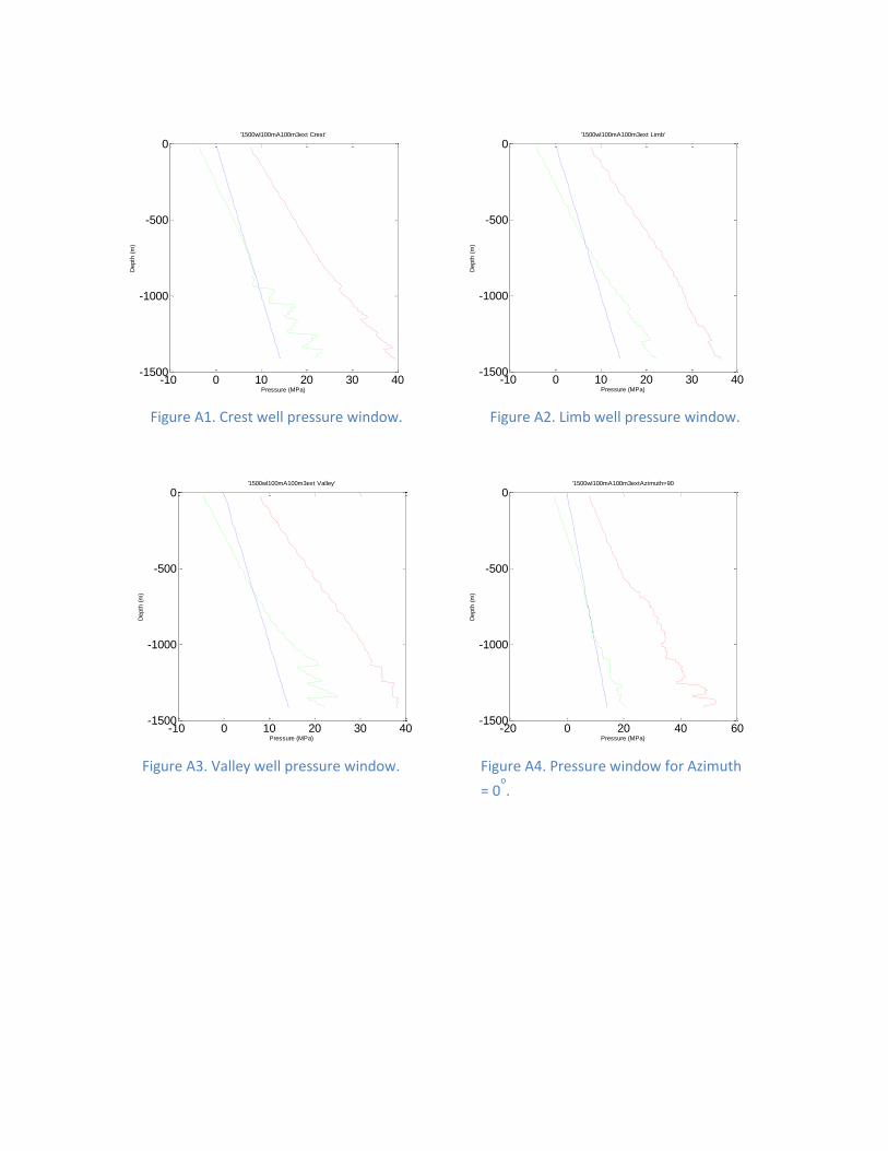
-10 0 10 20 30 40-1500
-1000
-500
0
Pressure (MPa)
Depth
(m
)'1500wl100mA100m3ext Crest'
-10 0 10 20 30 40-1500
-1000
-500
0
Pressure (MPa)
Depth
(m
)
'1500wl100mA100m3ext Limb'
Figure A1. Crest well pressure window. Figure A2. Limb well pressure window.
-10 0 10 20 30 40-1500
-1000
-500
0
Pressure (MPa)
Depth
(m
)
'1500wl100mA100m3ext Valley'
Figure A3. Valley well pressure window.
-20 0 20 40 60-1500
-1000
-500
0
Pressure (MPa)
Depth
(m
)
'1500wl100mA100m3extAzimuth=90
Figure A4. Pressure window for Azimuth
= 0o.
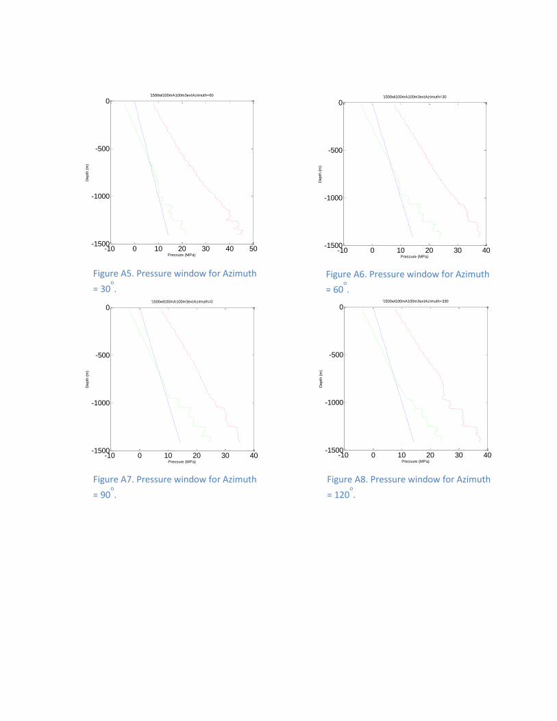
-10 0 10 20 30 40 50-1500
-1000
-500
0
Pressure (MPa)
Depth
(m
)
'1500wl100mA100m3extAzimuth=60
Figure A5. Pressure window for Azimuth
= 30o.
-10 0 10 20 30 40-1500
-1000
-500
0
Pressure (MPa)
Depth
(m
)
'1500wl100mA100m3extAzimuth=30
Figure A6. Pressure window for Azimuth
= 60o.
-10 0 10 20 30 40-1500
-1000
-500
0
Pressure (MPa)
Depth
(m
)
'1500wl100mA100m3extAzimuth=0
Figure A7. Pressure window for Azimuth
= 90o.
-10 0 10 20 30 40-1500
-1000
-500
0
Pressure (MPa)
Depth
(m
)
'1500wl100mA100m3extAzimuth=330
Figure A8. Pressure window for Azimuth
= 120o.

-10 0 10 20 30 40 50-1500
-1000
-500
0
Pressure (MPa)
Depth
(m
)
'1500wl100mA100m3extAzimuth=300
Figure A9. Pressure window for Azimuth
= 150o.
-20 0 20 40 60-1500
-1000
-500
0
Pressure (MPa)
Depth
(m
)
'1500wl100mA100m3extAzimuth=270
Figure A10. Pressure window for Azimuth
= 180o.
-10 0 10 20 30 40 50-1500
-1000
-500
0
Pressure (MPa)
Depth
(m
)
'1500wl100mA100m3extAzimuth=240
-10 0 10 20 30 40-1500
-1000
-500
0
Pressure (MPa)
Depth
(m
)'1500wl100mA100m3extAzimuth=210
Figure A12. Pressure window for Azimuth
= 240o.
Figure A11. Pressure window for Azimuth
= 210o.
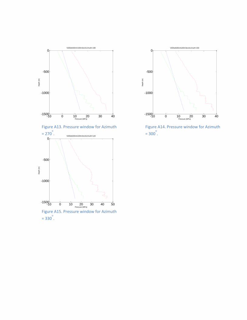
-10 0 10 20 30 40-1500
-1000
-500
0
Pressure (MPa)
Depth
(m
)
'1500wl100mA100m3extAzimuth=180
Figure A13. Pressure window for Azimuth
= 270o.
Figure A15. Pressure window for Azimuth
= 330o.
Figure A14. Pressure window for Azimuth
= 300o.
-10 0 10 20 30 40-1500
-1000
-500
0
Pressure (MPa)
Depth
(m
)
'1500wl100mA100m3extAzimuth=150
-10 0 10 20 30 40 50-1500
-1000
-500
0
Pressure (MPa)
Depth
(m
)
'1500wl100mA100m3extAzimuth=120
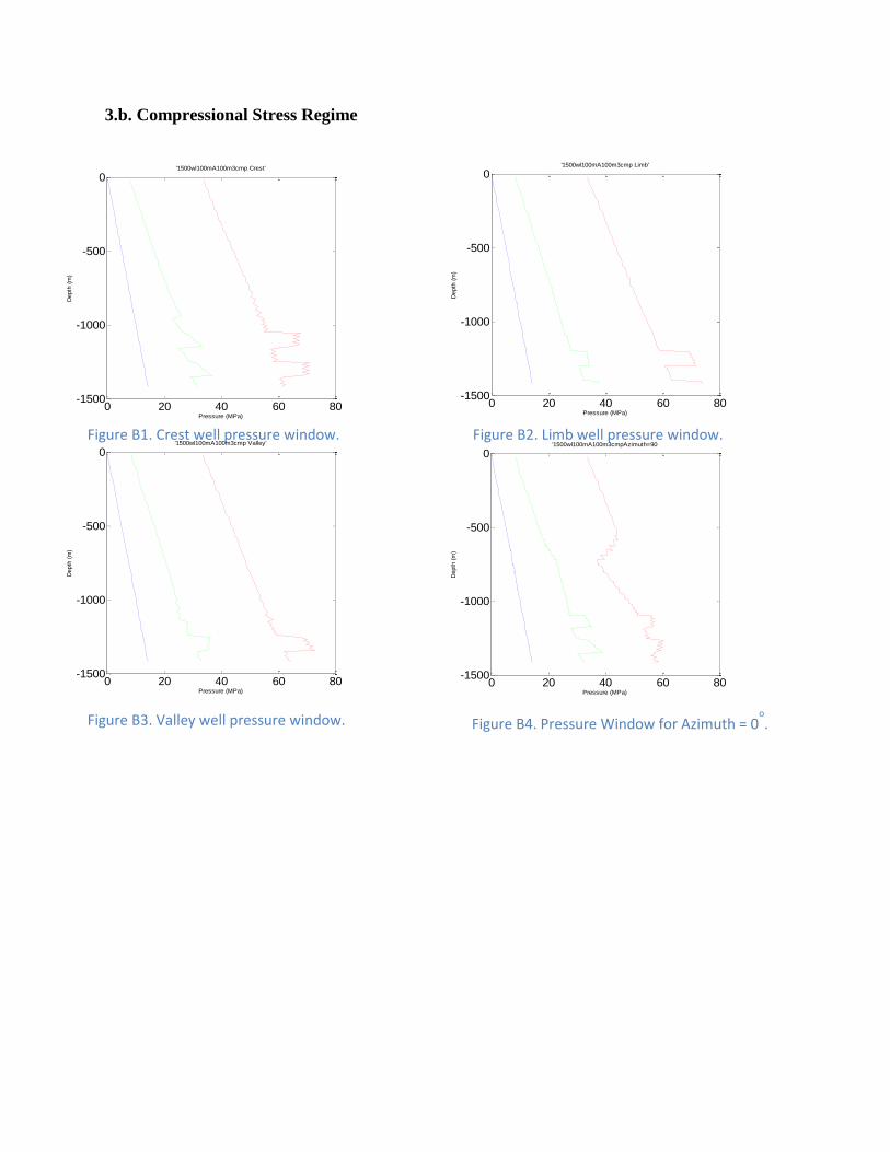
3.b. Compressional Stress Regime
0 20 40 60 80-1500
-1000
-500
0
Pressure (MPa)
Depth
(m
)
'1500wl100mA100m3cmp Crest'
Figure B1. Crest well pressure window. Figure B2. Limb well pressure window.
Figure B3. Valley well pressure window. Figure B4. Pressure Window for Azimuth = 0o.
0 20 40 60 80-1500
-1000
-500
0
Pressure (MPa)
Depth
(m
)
'1500wl100mA100m3cmp Limb'
0 20 40 60 80-1500
-1000
-500
0
Pressure (MPa)
Depth
(m
)
'1500wl100mA100m3cmp Valley'
0 20 40 60 80-1500
-1000
-500
0
Pressure (MPa)
Depth
(m
)
'1500wl100mA100m3cmpAzimuth=90

0 20 40 60 80-1500
-1000
-500
0
Pressure (MPa)
Depth
(m
)
'1500wl100mA100m3cmpAzimuth=60
Figure B7. Pressure Window for Azimuth = 90o. Figure B8. Pressure Window for Azimuth = 120
o.
Figure B6. Pressure Window for Azimuth = 60o. Figure B5. Pressure Window for Azimuth = 30
o.
0 20 40 60 80-1500
-1000
-500
0
Pressure (MPa)
Depth
(m
)
'1500wl100mA100m3cmpAzimuth=30
0 20 40 60 80-1500
-1000
-500
0
Pressure (MPa)
Depth
(m
)
'1500wl100mA100m3cmpAzimuth=0
0 20 40 60 80-1500
-1000
-500
0
Pressure (MPa)
Depth
(m
)
'1500wl100mA100m3cmpAzimuth=330
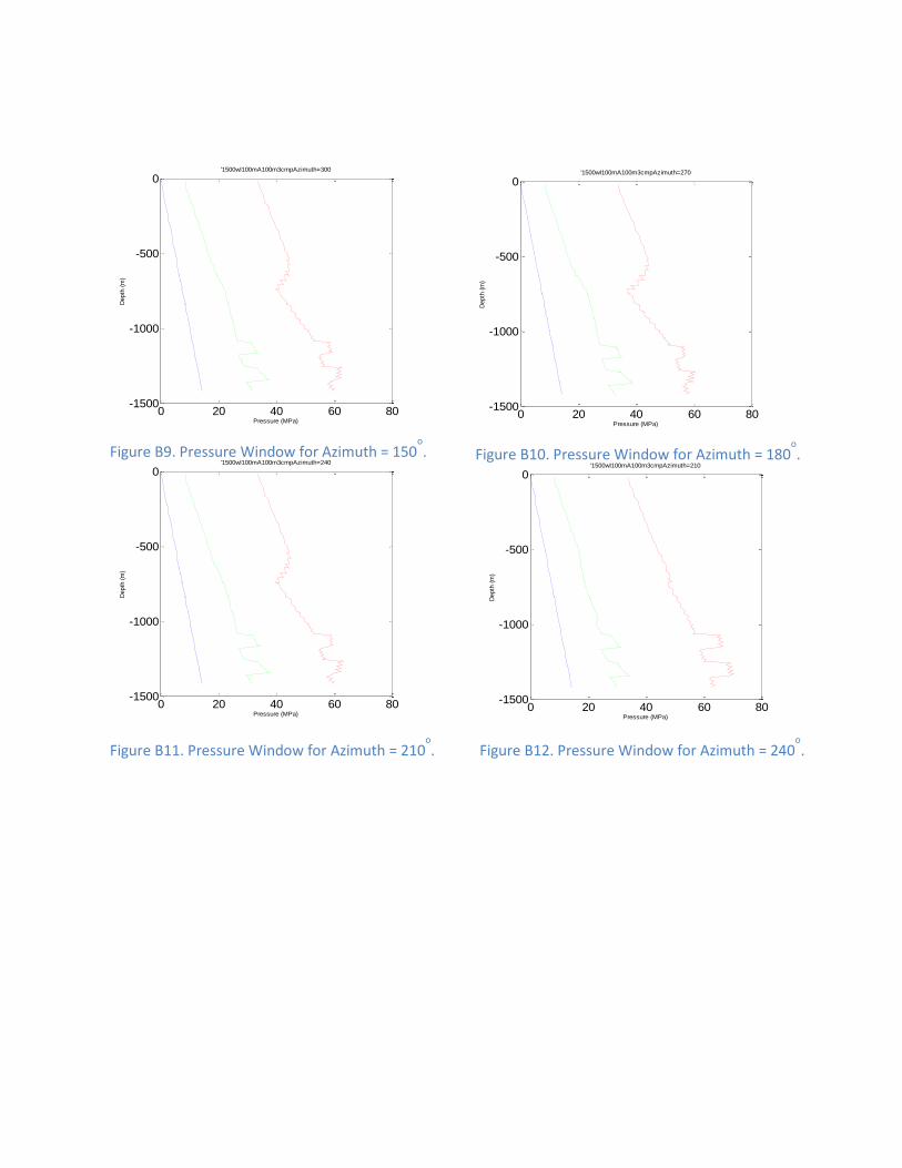
0 20 40 60 80-1500
-1000
-500
0
Pressure (MPa)
Depth
(m
)
'1500wl100mA100m3cmpAzimuth=300
Figure B12. Pressure Window for Azimuth = 240o. Figure B11. Pressure Window for Azimuth = 210
o.
Figure B10. Pressure Window for Azimuth = 180o. Figure B9. Pressure Window for Azimuth = 150
o.
0 20 40 60 80-1500
-1000
-500
0
Pressure (MPa)
Depth
(m
)
'1500wl100mA100m3cmpAzimuth=270
0 20 40 60 80-1500
-1000
-500
0
Pressure (MPa)
Depth
(m
)
'1500wl100mA100m3cmpAzimuth=240
0 20 40 60 80-1500
-1000
-500
0
Pressure (MPa)
Depth
(m
)
'1500wl100mA100m3cmpAzimuth=210

0 20 40 60 80-1500
-1000
-500
0
Pressure (MPa)
Depth
(m
)
'1500wl100mA100m3cmpAzimuth=180
Figure B15. Pressure Window for Azimuth = 330o.
Figure B14. Pressure Window for Azimuth = 300o. Figure B13. Pressure Window for Azimuth = 270
o.
0 20 40 60 80-1500
-1000
-500
0
Pressure (MPa)
Depth
(m
)
'1500wl100mA100m3cmpAzimuth=150
0 20 40 60 80-1500
-1000
-500
0
Pressure (MPa)
Depth
(m
)
'1500wl100mA100m3cmpAzimuth=120

3.c. Strike-Slip Stress Regime
0 10 20 30 40 50 60-1500
-1000
-500
0
Pressure (MPa)
Depth
(m
)
'1500wl100mA100m3ss Crest'
Figure C1. Crest well pressure window.
0 20 40 60 80-1500
-1000
-500
0
Pressure (MPa)
Depth
(m
)
'1500wl100mA100m3ss Limb'
Figure C3. Crest well pressure window.
Figure C2. Limb well pressure window.
-20 0 20 40 60-1500
-1000
-500
0
Pressure (MPa)
Depth
(m
)
'1500wl100mA100m3ss Valley'
-20 0 20 40 60 80-1500
-1000
-500
0
Pressure (MPa)
Depth
(m
)
'1500wl100mA100m3ssAzimuth=90
Figure C4. Pressure window for Azimuth
= 0o.
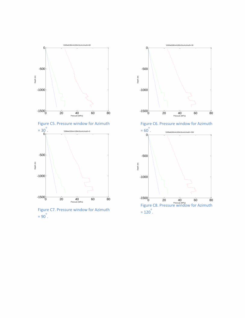
0 20 40 60 80-1500
-1000
-500
0
Pressure (MPa)
Depth
(m
)
'1500wl100mA100m3ssAzimuth=60
Figure C8. Pressure window for Azimuth
= 120o.
Figure C7. Pressure window for Azimuth
= 90o.
Figure C6. Pressure window for Azimuth
= 60o.
Figure C5. Pressure window for Azimuth
= 30o.
0 20 40 60 80-1500
-1000
-500
0
Pressure (MPa)
Depth
(m
)
'1500wl100mA100m3ssAzimuth=30
0 20 40 60 80-1500
-1000
-500
0
Pressure (MPa)
Depth
(m
)
'1500wl100mA100m3ssAzimuth=0
0 20 40 60 80-1500
-1000
-500
0
Pressure (MPa)
Depth
(m
)
'1500wl100mA100m3ssAzimuth=330
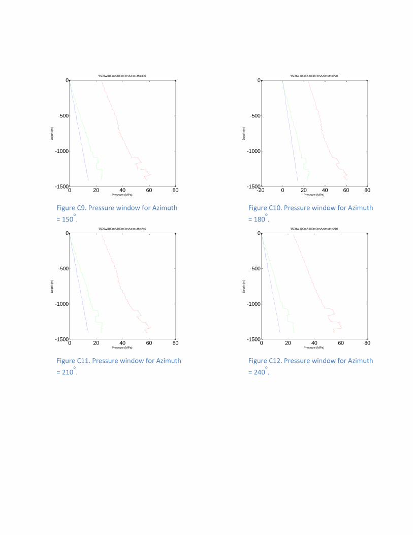
0 20 40 60 80-1500
-1000
-500
0
Pressure (MPa)
Depth
(m
)
'1500wl100mA100m3ssAzimuth=300
Figure C12. Pressure window for Azimuth
= 240o.
Figure C11. Pressure window for Azimuth
= 210o.
Figure C10. Pressure window for Azimuth
= 180o.
Figure C9. Pressure window for Azimuth
= 150o.
-20 0 20 40 60 80-1500
-1000
-500
0
Pressure (MPa)
Depth
(m
)
'1500wl100mA100m3ssAzimuth=270
0 20 40 60 80-1500
-1000
-500
0
Pressure (MPa)
Depth
(m
)
'1500wl100mA100m3ssAzimuth=240
0 20 40 60 80-1500
-1000
-500
0
Pressure (MPa)
Depth
(m
)
'1500wl100mA100m3ssAzimuth=210
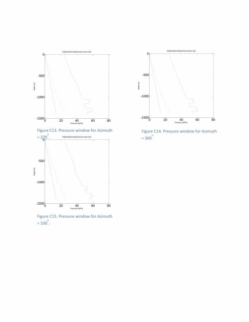
0 20 40 60 80-1500
-1000
-500
0
Pressure (MPa)
Depth
(m
)
'1500wl100mA100m3ssAzimuth=180
Figure C15. Pressure window for Azimuth
= 330o.
Figure C14. Pressure window for Azimuth
= 300o.
Figure C13. Pressure window for Azimuth
= 270o.
0 20 40 60 80-1500
-1000
-500
0
Pressure (MPa)
Depth
(m
)
'1500wl100mA100m3ssAzimuth=150
0 20 40 60 80-1500
-1000
-500
0
Pressure (MPa)
Depth
(m
)
'1500wl100mA100m3ssAzimuth=120