Embed Size (px)
Citation preview

57
4.1 Introduction
Porous bodies are aggregates of solid elements between which voids form the
pore space itself. These voids within the porous body give rise to the wide differences in
physical behavior between dense solids and porous substances, which are assemblages in
which the presence of the fluid adds to the overall complexity of the material [41]. In a
broad classification, porous materials can be described as either rigid framed or elastic
framed materials. Examples of rigid framed porous media are honeycomb core which
consists of narrow cavities that act as resonators and porous rock. Fiberglass and
acoustical foams are considered elastic framed porous materials. All of these materials are
heterogeneous in that they are comprised of a solid phase (often referred to as the frame)
and a fluid phase (see Figure 4.1). In dealing with the problem of acoustic wave
propagation in saturated, porous media for dynamic analysis of the subsurface, two
approaches are possible. The first approach is based on the homogenization principle [42]
which links the microscopic and macroscopic laws of sound propagation. The term
microscopic applies to laws governing mechanisms at the scale of heterogeneity.
Macroscopic laws refer to a scale related to the heterogeneous medium concerned. The
second approach consists of deliberately ignoring the microscopic level and assuming that
Chapter 4
Numerical Modeling of Smart Foam
Chapter 4 Numerical Modeling of Smart Foam 58
the concepts and principles of continuum mechanics can be applied to obtain measurable
macroscopic values. For this work, the author has decided to present an analysis of
porous media using a macroscopic approach since it has more physically realizable
assumptions. As illustrated in Figure 4.1, the basic premise of the theory requires that
there exists a macroscopic elementary volume or subdomain that is representative of the
porous media considered. The basic premise is that the pore size (d) is much smaller than
the macroscopic elementary volume of porous material (D1). It is also assumed that the
wavelength (D2) of sound propagating within the porous layer is much larger than the
pore space and the macroscopic elementary volume. Accordingly, it is possible to
establish average volume displacements per unit cross sectional area for the solid phase
ux uy uz and the fluid phase Ux Uy Uz of the porous layer which are common, easily-
handled physical properties.
x
y
z
Macroscopic Analysis: d<<D1<<D2
D1
Elemental Volumeof Porous Material
Solid Phase
ux uy uzFluid Phase
Ux Uy Uz
d
Acoustic wavetravelling within porous material
PorousMaterial
D2
Figure 4.1 Illustration of a generic porous material and the macroscopic modeling approach.
Porous acoustical materials are unique in that air represents the fluid phase of the
material. Acoustical foam, which is an essential component in this study can be described
by several macroscopic parameters. These parameters are the porosity, flow resistance,
the tortuosity, bulk density, Young’s modulus with associated loss factor and Poisson’s

Chapter 4 Numerical Modeling of Smart Foam 59
ratio. A description of some of these parameters and suggested measurement techniques
[43,44,45,46] are given in Table 4.1.
Table 4.1 Important foam parameters and measurement techniques.Foam Property & Definition Measurement TechniquePorosity: ratio of air volume/total volume ofporous material
pore volume measured directly by the difference indry and saturated weight in a vacuum
Flow resistivity: resistance to air flow per unitthickness
foam sample placed in a pipe; differential pressureinduced by a steady flow of air
Tortuosity: describes pores deviation from straightcylindrical passages
compare electrical conductivity of a conductivefluid with that of the foam sample saturated by thesame fluid
Young’s modulus & associated loss factor:stiffness of foam
compute the flexural response of a beam with andwithout the foam attached
There are three categories of porous acoustical foams. The categories are open
cell, partially-reticulated and closed cell foams. These three types are distinguished from
each other by the degree to which the cell membranes are removed during the
manufacturing process. The cell membranes are completely extracted in open cell foams.
Open cell foams tend to be quite limp and little coupling exists between the motion of the
solid and fluid phases. An example of an open cell foam is fiberglass which is commonly
used for building insulation. In partially-reticulated foams, only a portion of the cell
membranes are removed, the fluid propagation path tends to follow tortuous passages.
Partial foam reticulation results in an elevated frame stiffness and Poisson’s ratio in
comparison to open cell foams. A large tortuosity reduces the phase speed of the airborne
waves, but also increases the viscous and inertial effects that are present due to the strong
coupling between the motion of the solid phase and the interstitial fluid. Polyurethane
acoustical foam is an example of partially-reticulated porous material. Closed cell foams
are airtight and all the fluid is trapped within closed cells. They resemble homogeneous
elastic medium. Generally, poor acoustical properties are offered by closed cell foams.
Owing to these facts, noise control applications employ partially-reticulated acoustic
foams as passive sound absorbers in the high frequency range where the dissipative
mechanisms within the foam are significant [47, 48].
4.2 Overview of Poroelastic Material Theory Development

Chapter 4 Numerical Modeling of Smart Foam 60
The following discussion summarizes the work of key contributors in the
evolvement of theories related to wave propagation in poroelastic media. A complete
listing is beyond the scope of this thesis, however, a general historical description of
previous work is necessary in the interest of completeness.
In 1896, Rayleigh [49] presented the first published material on sound
propagation in air-saturated, porous media. He investigated the performance of an
idealized absorber of sound, consisting of a bundle of small tubes aligned in the direction
of wave propagation. He extended the theories of Helmholtz and Kirchoff that relate to
the transmission of sound along tubes and was able to deduce a value for the absorption
coefficient at the surface of the absorber in terms of the proportion of the surface area
occupied by open pores, the radius of the tubes and the physical constants of the air.
Although the solid component of the material was assumed to be rigid, this simple model
accounted for viscous and thermal losses in the pores which is a key feature in modern
models.
Zwikker & Kosten [50] were perhaps the earliest scientists to study sound
absorbing elastic materials. Unlike Rayleigh, they accounted for the possibility of
vibration of the solid material and addressed the mathematical problem of the coupled
vibrations of the solid and fluid phases. The phase coupling is attributed to fluid viscosity
and inertial effects created by a pore structure that deviated from straight cylindrical
passages. The Zwikker and Kosten approach predicts the presence of two longitudinal
wave types that are common to each phase of the porous material.
In 1956, Biot [51, 52, 53] advanced the theory of Zwikker and Kosten to describe
wave propagation in media related to geophysics. The model included shear stiffness of
the solid phase of an elastic porous material. Accordingly, the Biot theory predicted the
presence of two longitudinal wave types and one shear wave type in porous, elastic
media. It is the most general, elastic porous material theory available. Seven constitutive
equations are derived that relate stress and pressure in the frame and the fluid to the
coupled deformations of both phases. The constitutive equations are expressed in terms
of two Lame’ coefficients and two coupling coefficients. The viscous and inertial

Chapter 4 Numerical Modeling of Smart Foam 61
coupling effects are included in three effective densities. Six equations govern the motion
of the frame and fluid in three orthogonal directions.
Delaney & Bazely [54] presented empirical methods that have been widely used
for predicting sound propagation in various grades of fibrous materials. These laws have
been used in various applications such as sound attenuation in ducts, room acoustics, the
calculation of transmission loss through walls, and primarily models describing sound
propagation above various types of ground. The geometry of fibrous materials was not
taken into account.
The subject of shape factors as applied to the pore geometry of rigid porous
materials is addressed by Champoux and Stinson [55]. They accurately predicted the
complex density and propagation constant in rigid-framed porous materials having large
variations in pore cross-sectional area. They introduced the use of shape factors to treat
the effect of pore shape on the thermal and viscous functions. It is demonstrated that the
dynamic density function (that describes the viscous effects) is associated more with the
narrow sections of the pores and the dynamic bulk modulus (describing the thermal
effects) is associated more with the wider sections of the pores. Two different shape
factors are required, in general, to describe both the viscous and thermal effects. Very
good agreement between the experimental results and the theoretical predictions is found.
Attenborough [56] and Johnson et al. [57] have also contributed significantly to
the study of rigid porous materials with attention given to pore geometry.
Works by Allard [58, 59] were developed to adapt specifically the Biot theory to
acoustics problems involving mutilayered poroelastic media. His model includes two
characteristic dimensions for viscosity and the bulk modulus of air within the pores,
respectively. These parameters are dependent on the foam material properties and pore
shape factors.
Bolton et al. [60,61,62] published analytical studies based on the Biot theory
which deal with normal and oblique wave propagation in elastic porous materials with
it’s application to the prediction of the transmission loss of foam lined noise control
treatments.

Chapter 4 Numerical Modeling of Smart Foam 62
Early work related to absorptive finite elements was performed by Craggs [63, 64]
and related to lined rectangular rooms. The theory was derived from a generalized
Rayleigh model, but allowed for a frequency dependent flow resistivity and density. It
also considered the effects of porosity. The application of the theory shows good
agreement with experimental data taken for foam material and with the empirical formula
developed by Delaney and Bazely for effectively rigid materials. These comparisons were
carried out for normal incidence only and accounted for only one wavetype. It is now
known that three distinct wavetypes (i.e. two longitudinal and one shear wave) contribute
significantly to the acoustical behavior of poroelastic materials such as foams. Therefore,
Cragg’s approach is not appropriate for noise control foams.
Recently, Kang [65, 66] presented an elastic-absorption finite element model of
isotropic elastic porous noise control materials implementing a finite element approach.
The two-dimensional displacement based approach is founded on the Biot theory and
allows for the propagation of the three types of waves known to propagate in a poroelastic
material. The starting point of this formulation was the differential equations of dynamic
equilibrium. Next, the discretized poroelastic equations were derived using Galerkin’s
method. A method of coupling foam and acoustic finite elements is presented. The effects
of finite dimension and edge constraints on sound absorption and transmission through
layers of acoustical foam is studied. Good agreement is achieved when finite element
predictions are compared with established analytical plane wave absorption and
transmission loss.
Panneton [67, 68, 69] employed the finite element method to solve the three
dimensional poroelasticity problem related to sound absorption and transmission loss
based on the Biot theory. His work differs from Kang’s in that it is derived using a
Lagrangian approach. Furthermore, he gives attention to the efficiency (i.e. solution time
and memory requirements) of the numerical implementation by introducing realistic
approximations to remove the complex nature and frequency dependence of the
poroelastic material properties.
Chapter 4 Numerical Modeling of Smart Foam 63
4.3 Biot Theory of Sound Propagation in Isotropic, Elastic Porous Materials
The purpose of the present discussion concerning the analytical modeling of
sound wave propagation in porous materials undergoing an acoustic excitation is twofold.
Firstly, the model serves to identify the unique characteristics of porous materials. It is
shown that the presence of the fluid phase significantly effects the behavior of the
material when compared to a similar elastic, homogeneous medium. Two compressional
waves and one shear wave can travel within the foam. Derivation of the complex
wavenumbers, allows the phase speed and attenuation coefficient of each wavetype to be
studied as a function of frequency. The second function of the analytical formulation of
porous materials is to validate the finite element model. This will be accomplished by
comparing the acoustic impedance of partially-reticulated acoustic foam predicted by
each approach.
The theory describing acoustic wave propagation in an elastic porous material
filled with compressible viscous fluid is considered in the context of Biot theory as
presented by Allard [59]. As stated previously, this macroscopic approach utilizes the
concepts and principles of continuum mechanics [70] to obtain measurable macroscopic
values describing the dynamic behavior of the material. The major hypotheses of the Biot
theory are:
• the poroelastic subdomains are homogeneous and isotropic.
• the wavelength is large in comparison with the dimensions of the macroscopic
elementary volume.
• the pore space is small relative to the macroscopic elementary volume.
• deformations are small which guarantee linearity of the mechanical processes.
• viscous damping and heat transfer at the pore walls is considered.
• the fluid within the pores is initially at rest and the flow of fluid relative to the
solid is of Poiseuille type (i.e. the instantaneous velocity profile is parabolic).
After defining the stress-strain relations for both the solid phase and fluid phase and the
potential and kinetic energy expressions, the three dimensional dynamic equations of
motion are derived using Lagrange’s equations [71]. These equations contain three
effective mass coefficients reflecting the inertial coupling between the solid and fluid
Chapter 4 Numerical Modeling of Smart Foam 64
phase and the viscous dissipation present in the porous material. Biot theory identifies the
existence of two compressional waves and one shear wave.
4.3.1 Stress-Strain Relations
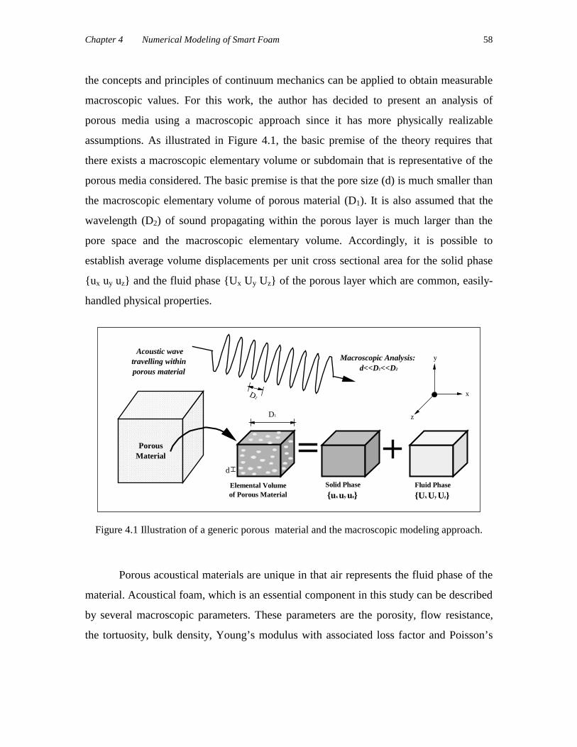
In an elastic solid or in a fluid, stresses are defined as being tangential or normal
forces per unit area of material. The same definition will be used for porous materials,
and stresses are defined as being forces acting on the frame or the air per unit area of
porous material as illustrated in Figure 4.2.
x
y
z
SOLID PHASEState of Stress
FLUID PHASEState of Stress
σ yys
σ xxs
σ yzs
σ yxs
σ xys
σ zys
σ zzs
σ zxs
σ xzs
σ yyf
σ xxf
σ zzf
Figure 4.2 State of stress in the solid and fluid phases of an elementary macroscopic volume ofporous material.
As a consequence, the stress tensor components for the solid are
σ σ σ σ σ σ σsxxs
yys
zzs
xys
yzs
zxs= (1)
The forces acting on the fluid part of each face of the cube are represented by
σ σ σ σfxxf
yyf
zzf= 0 0 0 (2)
The fluid stress components can be succinctly described by
σ β δij ijp= − (3)
where p denotes the pressure and β denotes the fraction of fluid area per cross section,
and δ ij is the Kronecker symbol defined as
δ ij
if i j
if i j=
≠=
0
1 (4)

Chapter 4 Numerical Modeling of Smart Foam 65
Note that σ f is taken negative when the force acting on the fluid is a pressure, and σ s is
positive when the force in the solid is a tension. It is important to call attention to the
significance of the factor β . In this analysis, it is assumed that we are dealing with a
statistically isotropic porous material in such a way that for all cross sections, the same
ratio of fluid area to solid area is observed. Hence the volume of fluid in a thin slab of
thickness dx is always a fraction β of the total volume. This means that β is identical to
the porosity, φ , or the ratio of fluid volume to total volume of the material. It is
important to note that σ σ σp s f= + or the total stress tensor of the poroelastic material
is the sum of the tensor related to the solid and fluid phase, respectively.
The strain tensor in the solid is denoted by
ε ε ε ε ε ε εsxxs
yys
zzs
xys
yzs
zxs= 2 2 2 (5)
where
( )ε ijs
i j j iu u= +1
2 , , (6)
We may also define the dilatation of the solid phase as
θ si iu= , (7)
where u=ux uy uz is the displacement vector of the solid. Keep in mind that the
displacement vector is defined as the displacement of the material which is considered to
be uniform and averaged over the element. Similarly, the average fluid displacement
vector U=Ux Uy Uz is defined so that the product of this displacement with the cross-
sectional fluid area represents the volume flow. The strain in the fluid is defined as
ε ε ε εfxxf
yyf
zzf= 0 0 0 (8)
where
ε δ δ δijf
k l ik jk klU= , (9)
and the fluid dilatation is
θ fi iU= , (10)

Chapter 4 Numerical Modeling of Smart Foam 66
It is important to note that ε ε εp s f= + or the total strain of the poroelastic material is
the sum of the tensor related to the solid and fluid phase, respectively, and has seven
components.
It is now necessary to establish a relationship between the stress and strain
components of the poroelastic material. Disregarding all dissipative forces and assuming
that the material is a conservative physical system which is in equilibrium when at rest,
any deformation is therefore a departure from the state of minimal potential energy. The
potential energy can be expressed by a positive definite quadratic form where the stress
components will then be linear functions of the six strain components. The potential
energy W per unit of material is given by
( )W ijs
ijs
ijf
ijf= +
1
2σ ε σ ε (11)
The stress-strain relations may be expressed as
σ∂∂ε
σ∂∂ε
ijs
ijs
ijf
ijf
W
W
=
= (12)
The seven by seven matrix of coefficients in the foregoing set of linear relations
constitute a symmetric matrix with twenty eight distinct coefficients [53]. These relations
are very much simplified if the assumption that the solid-fluid system is statistically
isotropic. In this case, the principal stress and principal strain directions coincide and the
stress-strain relations can be written for arbitrary directions as
( )σ θ θ δ ε δijs s f
ij ijs
ijA Q N= + + 2 (13a)
( )σ θ θ δ φ δijf s f
ij ijQ R p= + = − (13b)
In examining the significance of the coefficients of equations (13a,b), the terms A
and N correspond to the familiar Lame coefficients in the theory of elasticity and are of
positive sign. The coefficent N denotes the shear modulus of the material. The quantity Q
gives the contributions of the air dilatation to the stress in the frame, and of the frame
dilatation to the pressure variation in the air in the porous material. The quantity Q is the
potential coupling coefficient. The quantity R relates the fluid stress and strain. The

Chapter 4 Numerical Modeling of Smart Foam 67
“gedanken experiments”, performed by Biot et al. [72] provide an evaluation of the
elasticity coefficients A, N, Q and R. In the experiments, the material is subjected to pure
shear to establish the shear modulus of the solid phase. The other experiments determine
the expressions of A, Q and R as a function of three significant physical properties of the
material. These properties are the bulk modulus of the material in vacuo (Kb), the bulk
modulus of the elastic solid from which the frame is made (Ks), and the bulk modulus of
the air (Kf). For porous materials saturated by air, it is practical to assume that Kb/Ks<<<1
and Kf/Ks<<<1. Accordingly, using Allard’s notation the elasticity coefficients can be
described in terms of Kb and Kf such that
A N K Kb f= + +−4
3
1 2( )φφ
(14)
Q K f= −( )1 φ (15)
and
R K f= φ (16)
The rigidity of an elastic solid is commonly characterized by a shear modulus
and the Poisson’s ratio of the material. With regard to this, the bulk modulus Kb in
equation (14) can be evaluated by the following expression
KN v
vb =+
−2 1
3 1 2
( )
( ) (17)
The terms N and v represent the shear modulus and the Poisson coefficient,
respectively. The bulk modulus of the fluid phase is defined by
( )K
P
j Bj
Bf
o
o
o
=
− − + +
−
γ
γ γη
ωρρ ω
η1 1
81
162 2
2 21
ΛΛ
’
’ (18)
where Po is the atmospheric pressure, γ denotes the specific heat ratio, η is the viscosity
of the air, ρo is the density of the air, σ is the mean flow resistance, B 2 is the Prandtl
number and ω is the circular frequency. The value Λ’ denotes the characteristic
dimension for thermal effects and accounts for pore geometry.
4.3.2 Kinetic Energy Density

Chapter 4 Numerical Modeling of Smart Foam 68
The kinetic energy of the system per unit volume, using the average velocity
components as generalized coordinates, is expressed as
T u u u U u U U Ux y x x y y x y=
+
+ +
+
+
• • • • • • • •1
2211
2 2
12 22
2 2
ρ ρ ρ (19)
Note that the dot over u and U signify the first time derivative of the variable. The kinetic
energy expression is based on the fact that the material is statistically isotropic, therefore,
the orthogonal directions are equivalent and uncoupled dynamically. In equation (19), the
mass coefficients ρ11 and ρ22 are related to the mass density of the solid and the fluid
phases, respectively. The coefficient ρ12 considers the inertial interaction between both
phases. These coefficients are defined as
( )
ρ ρ ρρ φρ ρ
ρ φρ α
11 1 12
22 12
12 1
= −= −
= − −o
o o
(20)
whereα o denotes the tortuosity of the material and ρ1 .represents the density of the
homogeneous solid phase of the foam.
4.3.3 Dissipation Function
As stated earlier, it will be assumed that the flow of fluid relative to the solid
through the pores is of the Poiseulle type. The dissipation function may be written in a
homogenous quadratic form. Because of the assumed statistical isotropy, orthogonal
directions are uncoupled. The dissipation also vanishes when there is no relative motion
between the fluid and solid. The dissipation function is defined as
D b u U u Ux x y y= −
+ −
• • • •1
2
2 2
(21)
where the damping constant is given as
b j o= + ∞φ σα ηρ ωσ φ
22
2 2 214
Λ (22)
and Λ is the characteristic dimension for viscous forces taking into account pore
geometry. Also, the term α∞ denotes the limit of the tortuosity as ω tends to infinity.

Chapter 4 Numerical Modeling of Smart Foam 69
4.3.4 Equations of Motion for an Isotropic, Elastic Porous Material
Lagrange’s equations with viscous dissipation are denoted by
∂∂
∂
∂
∂
∂t
T
u
D
uq
i i
i• •
+
= (23a)
∂∂
∂
∂
∂
∂t
T
U
D
UQ
i i
i• •
+
= (23b)
The terms qi and Qi represent the elastic forces for the solid and fluid phase, respectively,
such that
qd
dx
Wi
j ijs ij j
s
i= =
∂∂ε
σ , , (24a)
Qd
dx
Wpi
j ijf ij j
fi= = = −
∂∂ε
σ φ, , (24b)
Substituting equations (19),(21) ,(24) into equations (23) yields
σ ρ ρij js
ii i i i i iu U b u U, = +
+ +
•• •• • •
2 (25a)
− = +
− +
•• •• • •φ ρ ρp u U b u Uj i i i i, 12 22 (25b)
Employing equations (6), (7), (9) and (10) and equation (13) in equation (25), we derive
the equations of dynamic equilibrium in terms of the solid and fluid phase displacement
such that
( )Nu A N u QU u Ui jj j ii j ii i i, , ,( ) ~ ~+ + + = − +ω ρ ρ211 12 (26a)
( )Qu Ru QU u Ui jj j ii j ii i i, , ,~ ~+ + = − +ω ρ ρ2
12 22 (26b)
where harmonic motion having an e j tω time dependence is assumed. In the above
equations,

Chapter 4 Numerical Modeling of Smart Foam 70
~
~
~
ρ ρω
ρ ρ ω
ρ ρω
11 11
22 22
12 12
= −
= −
= +
jb
jb
jb
(28)
These parameters take into account the inertial effects and viscous dissipation of the
porous material.
4.4 The Compressional Waves
As in the case of an elastic solid, the wave equations of the compressional and
rotational waves can be obtained by using scalar and vector displacement potentials,
respectively. Two scalar potentials for the frame and the air, Φ s and Φ f , are defined for
the compressional waves, giving
u s= ∇Φ (28a)
U f= ∇Φ (28b)
By employing the relation ∇∇ = ∇ ∇Φ2 2Φ in equations (26a) and (26b), it can be shown
that Φ s and Φ f are related as follows:
( )( )
− + = ∇ + ∇
− + = ∇ + ∇
ω ρ ρ
ω ρ ρ
211 12
2 2
222 12
2 2
~ ~
~ ~Φ Φ Φ Φ
Φ Φ Φ Φ
s f s f
f s f s
P Q
R Q (29)
where
P A N= + 2 (30)
The two scalar potentials may be used to define the following vector
[ ] [ ]Φ Φ Φ= s f T (31)
Equations (29) can then be reformulated as
[ ] [ ][ ] [ ]− = ∇−ω ρ2 1 2M Φ Φ (32)
where
[ ] [ ]ρρ ρρ ρ=
=
~ ~
~ ~ ,11 12
12 22
MP Q
Q R (33)
Chapter 4 Numerical Modeling of Smart Foam 71
Allow δ12 and δ2
2 to define the eigenvalues, and [ ]Φ1 and [ ]Φ 2 the eigenvectors, of the
left-hand side of equation (32). These quantities are related by
[ ] [ ][ ] [ ]
− = ∇
− = ∇
δ
δ12
12
1
22
22
2
Φ Φ
Φ Φ (34)
The eigenvaluesδ12 and δ2
2 are the squared complex wavenumbers of the two
compressional waves, and are given by
( )[ ]δω
ρ ρ ρ12
2
2 22 11 1222=
−+ − −
PR QP R Q~ ~ ~ ∆ (35a)
( )[ ]δ ω ρ ρ ρ22
2
2 22 11 1222=
−+ − +
PR QP R Q~ ~ ~ ∆ (35b)
where
( ) ( )( )∆ = + − − − −P R Q PR Q~ ~ ~ ~ ~ ~ρ ρ ρ ρ ρ ρ22 11 12
2 211 22 12
22 4 (36)
The chosen determination of the square root in equations (35a) and (35b) is the one with
the positive real part. The two eigenvectors can be written
[ ] [ ]ΦΦΦ
ΦΦΦ1
1
12
2
2
=
=
s
f
s
f, (37)
By employing equation (29), the following equation gives the ratio of the velocity of the
frame over the velocity of the air for the two compressional waves and indicates what
medium the waves propagate in preferentially
µδ ω ρ
ω ρ δii
i
P
Qi=
−−
=2 2
112
122 1 2
~
~ , (38)
Four characteristic impedances can be defined since both wave simultaneously
propagate in the air and the frame of the porous material. The characteristic impedance
related to a wave propagating in the positive x direction in the air is denoted by
Zp
j uf
xf=
ω (39)
Substituting equations (13b) in equation (39), the characteristic impedance related to the
air can be rewritten as for the two compressional waves as

Chapter 4 Numerical Modeling of Smart Foam 72
( )Z R Q iif
ii= + =µ
δφω
, ,1 2 (40)
Similarly, the characteristic impedance related to a forward propagating wave in the solid
is denoted by
Zj u
s xxs
xf=
− σω
(41)
Substituting equations (13a) in equation (41), the characteristic impedance related to the
solid phase can be rewritten as for the two compressional waves as
( )Z P Q iis
ii= + =µ
δω
, ,1 2 (42)
4.5 The Shear Wave
As in the case for an elastic solid, the wave equation for the rotational wave can
be obtained by using vector potentials. Two vector potentials, Ψs and Ψ f , for the frame
and for the air, are defined as follows:
u s= ∇ × Ψ (43a)
U f= ∇ × Ψ (43b)
Substitution of the displacement representation, equations (43a) and (43b), into equations
(26a) and (26b) yields
( )− + = ∇ω ρ ρ211 12
2~ ~Ψ Ψ Ψs f sN (44a)
( )− + =ω ρ ρ212 22 0~ ~Ψ Ψs f (44b)
The wave equation is denoted by
∇ +−
=2
211 11 12
2
11
0Ψ Ψω ρ ρ ρ
ρN
~ ~ ~
~ (45)
The squared wavenumber for the shear wave is defined as
δω ρ ρ ρ
ρ32
211 22 12
2
22
=−
N
~ ~ ~
~ (46)
and the ratio of amplitudes of the displacement of the air and the fluid is given by

Chapter 4 Numerical Modeling of Smart Foam 73
µρ
ρ312
22
=− ~
~ (47)
Employing the three Biot wavenumbers and the coupling coefficients we can use the
traveling wave approach to establish the displacements within the foam. This analytical
approach will be demonstrated after a more in depth study of these wavenumbers and
their physical characteristics is presented.
4.6 The Three Biot Waves in Air-Saturated Acoustic Foam
The following discussion concerning the wave velocities and attenuation
coefficients of the three wave types common to porous media will be in the context of
partially reticulated acoustic foam, an integral part of this study. The material properties
for a typical partially reticulated acoustic foam is listed in Table 4.3. In this case, a strong
coupling exists between the fluid and the frame of the porous layer. The two
compressional waves exhibit very different properties and are identified as the fast wave,
or P1 wave, and the slow wave, or P2 wave. These waves correspond to classic
compressional waves. In the absence of the fluid, only one compressional wave exists.
The shear wave, sometimes referred to as the S wave, propagates within the frame of the
porous media since fluid does not support shear [40]. The foundation for these
distinctions are due to the fact that the ratio µ of the velocities of the fluid and the frame
is close to 1 for the fast wave, while these velocities are nearly opposite for the slow
wave. Also, the damping due to viscosity is much stronger for the slow wave relative to
the fast wave. (The characteristic dimensions for partially reticulated polyurethane foam
are Λ = −28 10 6x and Λ’= −320 10 6x ).

Chapter 4 Numerical Modeling of Smart Foam 74
Table 4.3: Typical properties of partially-reticulated acoustic foam.
Properties of Partially-reticulated foamFlow Resistivity, σ (Ns/m) 25.0x10³
Porosity, φ 0.90
Tortuosity, ε ’ 7.8
Poisson’s ratio, v 0.4
Shear modulus, N (N/m2) 286x103
Loss factor, η 0.265
Solid mass density, ρs30.0
Fluid mass density, ρf1.213
Consider the case of forward propagating acoustic wave and adopting an
exp( ~)j t krω − sign convention, the complex wavenumber can be defined as k j= −β α ,
where β is the phase constant, α is the attenuation coefficient, and both parameters have
a positive real part. The real part is related to the velocity of the wave which is given by
c = ω β . The wave speed can be expressed in non-dimensional form by normalizing the
value with respect to the speed of sound in air under standard conditions. Recall that
wavelength is defined as λ π β= 2 . The attenuation can be described in dimensionless
form as αλ πα β= 2 , which represents the attenuation per wavelength.
The normalized wave speeds for the three wave types propagating in partially
reticulated foam, using the material properties of Table 4.2, are plotted in Figure 4.3(a) as
a function of frequency. Observing the P1 wave, it appears that it’s speed is virtually
independent of frequency. It has a value of approximately 0.731 or 250.69 m/s. An
important conclusion can be drawn concerning the P1 wave when it’s speed is compared
to that of a compressional wave traveling in the equivalent homogeneous elastic medium.
The phase speed of the equivalent homogeneous elastic medium is given by c P= ρ1
or 239.27 m/s. Note that P, represents the elasticity coefficient of the frame in a vacuum
and is defined by equation (30) and ρ1 is the density of the material that constitutes the
solid phase. It can be concluded that the P1 wave corresponds to the frame wave. Note
that the presence of the fluid in the pores of the materials increases the stiffness of the
bulk material. Consequently, the frame wave in the elastic porous material is faster than

Chapter 4 Numerical Modeling of Smart Foam 75
the corresponding wave in a homogeneous elastic material possessing the same bulk
modulus as the in vacuo porous material.
In Figure 4.3(a), the P2 wave exhibits very different behavior when compared to
the P1 wave. It increases from a very small value in the low frequency region and
approaches an asymptotic limit of 0.3212 or 110.17 m/s in the high frequency region.
The asymptotic limit of the phase speed for the porous material with a rigid frame is
determined by c R= ~ρ22 , and this value is 113.85 m/s. Note that R describes the
elasticity coefficient of the fluid phase, defined by equation (16), and ~ρ22 is the mass
coefficient of the fluid phase defined in equation (28). This limiting value depends on the
inertial parameter known as the tortuosity [32]. It is evident that the P2 wave corresponds
to the airborne wave due to it’s similarity to the wave that propagates in a fluid
component of a rigid porous medium. In the present case, the finite frame elasticity has
the effect of reducing the phase velocity of the airborne wave below the value it would
have in an equivalent rigid porous material.
The phase speed of the shear wave or P3 wave in the foam is practically
independent of frequency, as shown in Figure 4.3(a), is equal to 0.287 or 98.56 m/s. The
shear wave speed in the homogeneous elastic medium is described by c N= ρ1 or
97.64 m/s. This observation supports the fact that the shear wave is strictly a frame wave
since fluids do not undergo shearing effects. Considering the three possible wave-types
common to partially-reticulated acoustic foam, the frame wave is the faster of the three
waves. Unlike other porous materials such as glass wool, the coupling of the solid and
fluid phase motion cannot be neglected in acoustic foams.

Chapter 4 Numerical Modeling of Smart Foam 76
102 103 1040.0
0.1
0.2
0.3
0.4
0.5
0.6
0.7
0.8
0.9
P1 wave P2 wave S wave
Nor
mal
ized
pha
se s
peed
Frequency (Hz)
Figure 4.3(a): Variation of the normalized phase speed of the P1, P2 and S waves propagating inacoustic foam with respect to frequency.
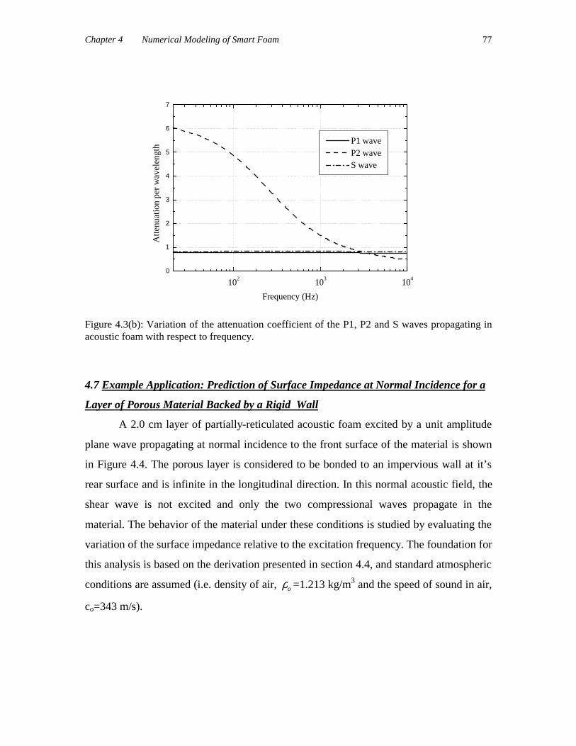
The attenuation per wavelength for the three wave-types is plotted in Figure 4.3(b)
as a function of frequency. Recall that this quantity is dimensionless and is described by
αλ πα β= 2 . The attenuation per wavelength of the frame wave (or P1 wave) and the
shear wave (or P3 wave) exhibit little frequency dependence possessing approximate
values of 0.7618 and 0.8205, respectively. In contrast the attenuation per wavelength of
the airborne wave (or P2 wave) decreases monotonically from large values at low
frequencies. It becomes smaller than the other values above 4000 Hz In the low
frequency region The airborne wave is the most heavily damped among the three
wavetypes. Accordingly, any foam lined noise control treatment in which the major
portion of the acoustical energy is carried through the lining by the airborne wave can be
expected to give good performance since a relatively large amount of energy will be
dissipated as the wave travels through the foam. These observations related to the wave
speeds and attenuation coefficients have also been predicted by other theoretical models
based on the Biot theory concerning wave propagation in acoustic foams [74].
Chapter 4 Numerical Modeling of Smart Foam 77
102 103 1040
1
2
3
4
5
6
7
P1 wave P2 wave S wave
Atte
nuat
ion
per
wav
elen
gth
Frequency (Hz)
Figure 4.3(b): Variation of the attenuation coefficient of the P1, P2 and S waves propagating inacoustic foam with respect to frequency.
4.7 Example Application: Prediction of Surface Impedance at Normal Incidence for a
Layer of Porous Material Backed by a Rigid Wall
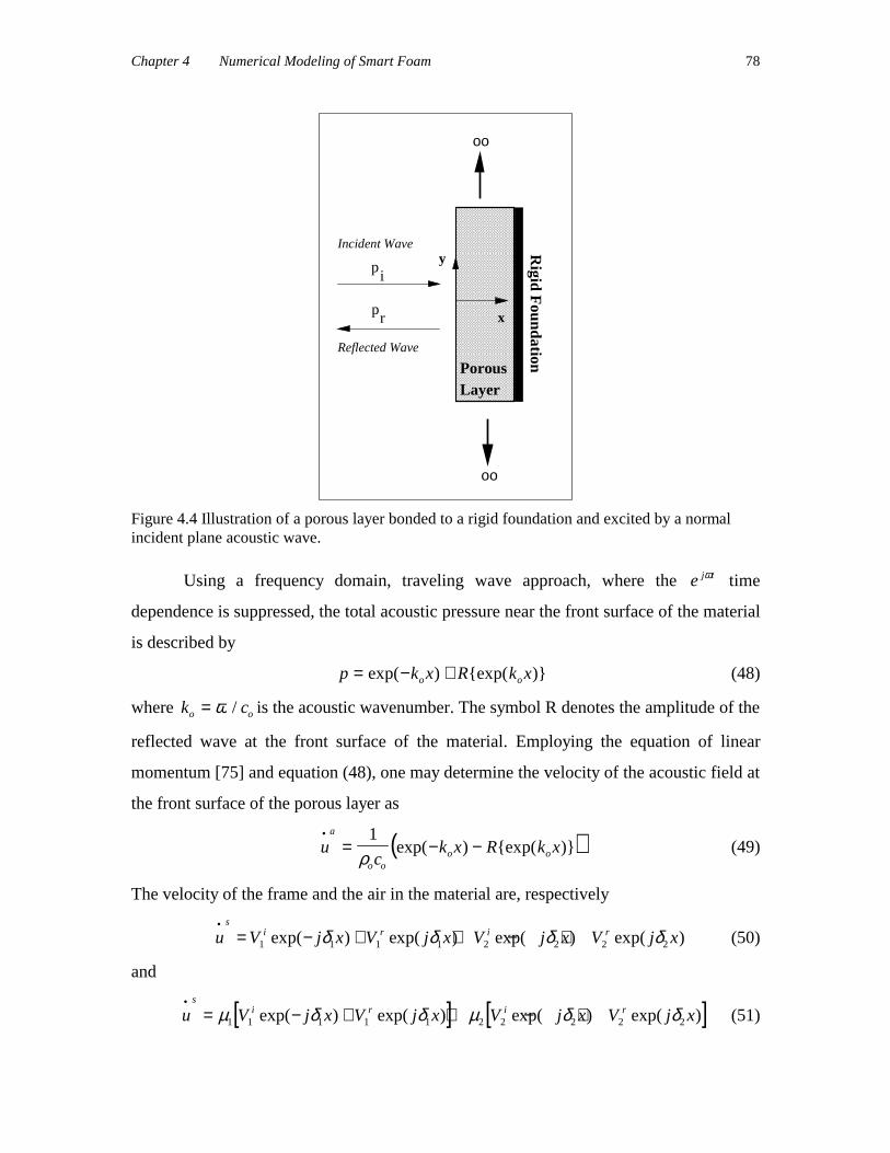
A 2.0 cm layer of partially-reticulated acoustic foam excited by a unit amplitude
plane wave propagating at normal incidence to the front surface of the material is shown
in Figure 4.4. The porous layer is considered to be bonded to an impervious wall at it’s
rear surface and is infinite in the longitudinal direction. In this normal acoustic field, the
shear wave is not excited and only the two compressional waves propagate in the
material. The behavior of the material under these conditions is studied by evaluating the
variation of the surface impedance relative to the excitation frequency. The foundation for
this analysis is based on the derivation presented in section 4.4, and standard atmospheric
conditions are assumed (i.e. density of air, ρo =1.213 kg/m3 and the speed of sound in air,
co=343 m/s).
Chapter 4 Numerical Modeling of Smart Foam 78
oo
oo
x
yp
p
i
r
PorousLayer
Rigid F
oundation
Incident Wave
Reflected Wave
Figure 4.4 Illustration of a porous layer bonded to a rigid foundation and excited by a normalincident plane acoustic wave.
Using a frequency domain, traveling wave approach, where the e j tω time
dependence is suppressed, the total acoustic pressure near the front surface of the material
is described by
p k x R k xo o= − +exp( ) exp( ) (48)
where k co o= ω / is the acoustic wavenumber. The symbol R denotes the amplitude of the
reflected wave at the front surface of the material. Employing the equation of linear
momentum [75] and equation (48), one may determine the velocity of the acoustic field at
the front surface of the porous layer as
( )uc
k x R k xa
o oo o
•= − −
1
ρexp( ) exp( ) (49)
The velocity of the frame and the air in the material are, respectively
u V j x V j x V j x V j xs
i r i r•
= − + + − +1 1 1 1 2 2 2 2exp( ) exp( ) exp( ) exp( )δ δ δ δ (50)
and
[ ] [ ]u V j x V j x V j x V j xs
i r i r•
= − + + − +µ δ δ µ δ δ1 1 1 1 1 2 2 2 2 2exp( ) exp( ) exp( ) exp( ) (51)

Chapter 4 Numerical Modeling of Smart Foam 79
The wavenumbers δ1 and δ2 are defined in equations (35), and µ1 and µ2 by equations
(38). The quantities Vi1 and Vr
1 are the velocities of the frame at x=0 associated with the
incident and reflected P1 wave. Similarly, the quantities Vi2 and Vr
2 are the velocities of
the frame at x=0 associated with the incident and reflected P2 wave. The stresses in the
solid and fluid phase of the material are given by
[ ] [ ]σ δ δ δ δxxs s i r s i rZ V j x V j x Z V j x V j x= − − − − − −1 1 1 1 1 2 2 2 2 2exp( ) exp( ) exp( ) exp( ) (52)
and
[ ] [ ]σ φ µ δ δ φ µ δ δxxs s i r s i rZ V j x V j x Z V j x V j x= − − − − − −1 1 1 1 1 1 2 2 2 2 2 2exp( ) exp( ) exp( ) exp( )
(53)
The unknown wave amplitudes can be evaluated by enforcing the boundary
conditions which ensure continuity of pressure and continuity of velocity at the front
surface of the material and set the velocities equal to zero at the porous material-wall
interface. These boundary conditions are :
x
p
p
u u u
x L u
u
xxs
xxf
f s a
s
f
=
= − −
= −
+ − =
= =
=
• • •
•
•
0
1
1
0
0
σ φσ φ
φ φ
( )
( )
(54)
Applying these five boundary conditions, the unknown wave amplitudes representing the
reflected wave in the air ( )R and the four incident and reflected waves associated with
the porous layer ( )V V V Vi r i r1 1 2 2, , , can be determined. Once these wave amplitudes are
established, the surface impedance can be calculated using
Zp x
u xa=
=
=•
( )
( )
0
0 (55)
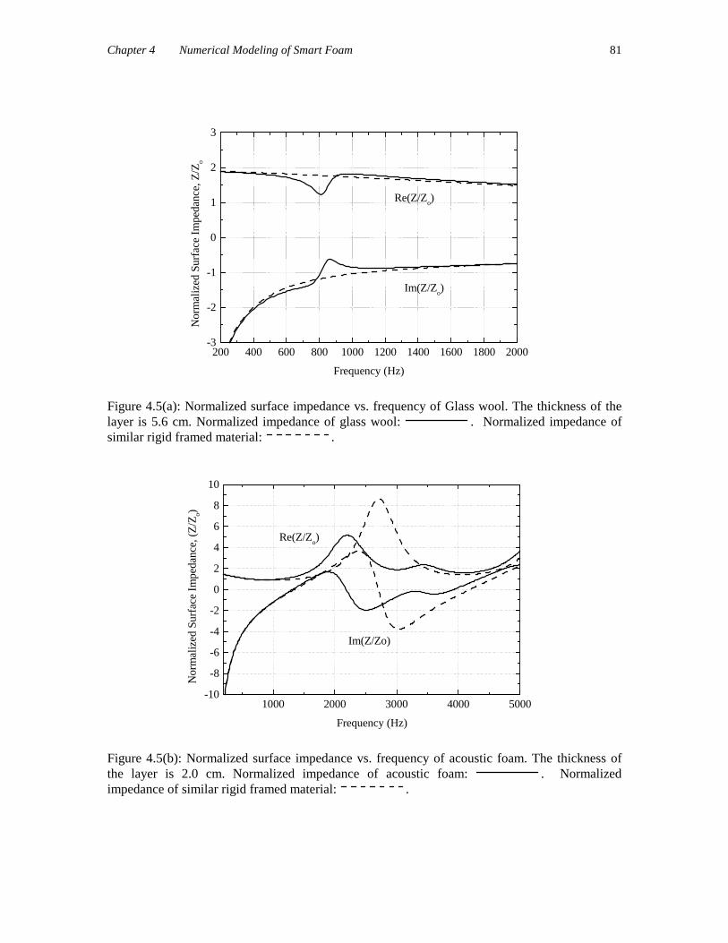
It is interesting to compare the surface impedance exhibited by the glass wool
termed ‘Domisol Coffrage’ and partially-reticulated acoustic foam; two different air-

Chapter 4 Numerical Modeling of Smart Foam 80
saturated porous materials. The glass wool properties are summarized in the Table 4.2.
The characteristic dimension values for glass wool are Λ = −0 56 10 4. x and Λ’ .= −112 10 4x .
The normalized surface impedance for a slab of the glass wool is plotted in Figure 4.5(a)
as a function of frequency up to 2000 Hz. A secondary set of curves representing the
prediction of the impedance of a similar material with a rigid frame are also plotted. (This
plot shows excellent agreement with the one presented by Allard [19] for the same
material). The frame resonance occurs when the real part of the impedance reaches a
minimum at 821.3 Hz. The normalized surface impedance for a layer of partially-
reticulated acoustic foam is plotted in Figure 4.5(b) as a function of frequency up to 2000
Hz. A secondary set of curves representing the prediction of the impedance of a similar
material with a rigid frame are also plotted. The frame of acoustic foam is lighter and less
stiff than that of glass wool, and this creates a stronger coupling between the solid and
fluid phase of the material. This characteristic is evident in Figure 4.5(b) which shows
that the frame wave cannot be ignored over the entire frequency range.
Table 4.2: Typical properties of glass wool.
Properties of Glass Wool ‘Domisol Coffrage’Flow Resistivity, σ (Ns/m) 40.0x10³
Porosity, φ 0.94
Tortuosity, ε ’ 1.06
Poisson’s ratio, v 0.0
Shear modulus, N (N/m2) 220.0x10⁴
Loss factor, η 0.1
Solid mass density, ρs (kg/m3) 130.0
Fluid mass density, ρf (kg/m3) 1.213
Chapter 4 Numerical Modeling of Smart Foam 81
200 400 600 800 1000 1200 1400 1600 1800 2000-3
-2
-1
0
1
2
3
Re(Z/Zo)
Im(Z/Zo)
Nor
mal
ized
Sur
face
Im
peda
nce,
Z/Z
o
Frequency (Hz)
Figure 4.5(a): Normalized surface impedance vs. frequency of Glass wool. The thickness of thelayer is 5.6 cm. Normalized impedance of glass wool: . Normalized impedance ofsimilar rigid framed material: .
1000 2000 3000 4000 5000-10
-8
-6
-4
-2
0
2
4
6
8
10
Im(Z/Zo)
Re(Z/Zo)
Nor
mal
ized
Sur
face
Im
peda
nce,
(Z
/Zo)
Frequency (Hz)
Figure 4.5(b): Normalized surface impedance vs. frequency of acoustic foam. The thickness ofthe layer is 2.0 cm. Normalized impedance of acoustic foam: . Normalizedimpedance of similar rigid framed material: .

Chapter 4 Numerical Modeling of Smart Foam 82
4.8 The Finite Element Method
The finite element method is a numerical procedure for analyzing structures and
continuum when the problem is too complicated to be solved satisfactorily by classical
analytical methods. The basic concept of the finite element method is discretization or
modeling a continuum as an assemblage of small parts or elements. Each element is of a
simple geometry and therefore is much easier to analyze than the actual structure. In
essence, a complicated solution may be approximated by a model that consists of
piecewise continuous simple solutions. The body analyzed can have arbitrary shape, loads
and support conditions. The mesh can mix elements of different types, shapes, and
physical properties. Another attractive feature of the finite element method (FEM) is the
close physical resemblance between the actual structure and its finite element model. The
model is not simply an abstraction. It is for these reasons that the finite element method is
chosen to analyze smart foam, which is a composite poroelastic-piezoelectric system
operating in an acoustic environment.
The finite element smart foam model is a linear approach which allows some
assessment of linearity of the actual system when comparing the model predictions with
experimental measurements. Furthermore, the finite element approach can be used to
optimize the smart foam configuration with a reasonable degree of confidence and
establish an active noise control simulation with smart foams.
Figure 4.7 illustrates a two-dimensional finite element model of a smart foam
actuator enclosed in an air-filled duct. It is assumed that the walls of the duct are rigid and
the actuator is excited by a voltage which generates sound propagation within the duct.
The goal is to discretize the system into a finite number of elements and determine the
resulting foam displacement and sound pressure field in the enclosure. The macroscopic
foam displacement field and acoustic pressure are interpolated from the nodal degrees of
freedom of the elements through the use of a shape function matrix, [N]. For example, the
macroscopic air pressure pe is defined as p N p
e e= [ ] where p
eis a vector of the
pressure at the nodes of the element. The acoustic foam and air cavity are discretized
using linear triangular finite elements [76] as shown in Figure 4.6. Linear triangular
elements are used because of their simplicity and the fact that the element shape function

Chapter 4 Numerical Modeling of Smart Foam 83
provides interelement continuity of the displacement field and it’s first derivative. Note
that the acoustic elements that discretize the airspace are uniformly distributed however,
the foam elements are non-uniformly distributed to account for the piezoelectric actuator.
As shown in Figure 4.6, the curved piezoelectric actuator (identified by the red line) is
approximated using a collection of plane truss elements [76] which account for axial
deformation. The axial deformation simulates the piezoelectric effect that occurs under
electrical excitation of the actuator.
Discretized Air CavityAcoustic System
DiscretizedSmart FoamPoroelastic-Piezoelectric System
y
x Note: Red line represents piezoelectric actuator
Figure 4.6. Illustration of discretized finite element model of smart foam in an air-filled duct.

Chapter 4 Numerical Modeling of Smart Foam 84
The smart foam numerical model is programmed in MATLAB® by the author
using the following steps:
(1) Mesh generation or dividing the system into finite elements, numbering theelements and corresponding nodes.
(2) Formulate the properties of each element by determining the nodal loads
associated with all element deformation states. (3) Assemble elements to determine the finite element model of the total system. (4) Apply known applied loads or moments. (5) Specify how the system is supported or set several nodal displacement to
known values. (6) Solve simultaneous linear algebraic equations to determine nodal degrees of
freedom. (7) Calculate element field variables from nodal degrees of freedom.
4.9 Finite Element Formulation for Poroelastic Media
In this section, a Lagrangian approach is combined with finite element
discretization to obtain the discretized equations of motion for a poroelastic medium [59,
67]. For two-dimensional analysis, four degrees of freedom per node are used to define
the displacement in the horizontal and vertical directions of each phase of the porous
medium. The kinetic energy density for a poroelastic medium is defined as
dT u u u U u U U Ux y x x y y x y=
+
+ +
+
+
• • • • • • • •1
2211
2 2
12 22
2 2
ρ ρ ρ (56)
and the strain energy density is defined as
dV s
T
s f
T
f= +
1
2σ ε σ ε (57)
where the stress tensors in the solid and fluid phase are represented by
[ ] [ ] σ ε εs s s sf fD D= + (58)
and

Chapter 4 Numerical Modeling of Smart Foam 85
[ ] [ ] σ ε εf f f sf sD D= + (59)
where [ ]Ds , [ ]D f and [ ]Dsf denote the elasticity tensors related to the solid phase, the
fluid phase and the strain coupling between both phases, respectively. These elasticity
tensors can be written as
[ ]D
A N A
A A N
Ns =
++
2 0
2 0
0 0
(60)
and
[ ]D Rf =
1 1 0
1 1 0
0 0 0
(61)
and
[ ]D Qsf =
1 1 0
1 1 0
0 0 0
(62)
The strain-displacement relations are
[ ] εs L u= (63)
and
[ ] ε f L U= (64)
where
[ ]L
x
y
y
x
=
∂ ∂
∂ ∂∂ ∂∂ ∂
0
0
(65)
Substituting equations (58)-(65) into equation (57) yields
[ ] ( ) [ ][ ] [ ] ( ) [ ][ ] [ ] ( ) [ ][ ] ( )dV L u D L u L u D L U L U D L UT
s
T
sf
T
f= + +1
22 (66)
The dissipation energy is
D b u U u Ux x y y= −
+ −
• • • •1
2
2 2
(67)

Chapter 4 Numerical Modeling of Smart Foam 86
Defining an external surface force as f f fx y
T
= , the work done per unit area by this
surface force on the poroelastic layer is defined as
dW f u f UT T
= − +( )1 φ φ (68)
Discretizing the poroelastic domain into classical linear triangular finite elements
[35] and interpolating the macroscopic displacement fields, u and U , in terms of the
nodal displacement u and U , yield for the eth element
[ ] u N ueu
e eT
= (69)
and
[ ] u N UeU
e eT
= (70)
By substituting equations (69)-(70) into (56),(66), and (67), the discretized energy
densiies and work expressions are obtained. Next integrating over the domain of each
element, summing the contribution from all elements and employing Lagrange’s
equations, the global discretized equations of motion are obtained
[ ] [ ][ ] [ ]
[ ] [ ][ ] [ ]−
+
=
ω 2M M
M M
K K
K K
u
U
F
Fss sf
sf ff
ss sf
sf ff
s
f
(71)
Specifically, the components of equation (71) are defined as
[ ] [ ] [ ]
[ ] [ ] [ ]
[ ] [ ] [ ]
[ ] [ ][ ] [ ][ ][ ]
[ ] [ ][ ] [ ][ ][ ]
[ ] [ ][ ] [ ][ ][ ]
M N N dA
M N N dA
M N N dA
K L N D L N dA
K L N D L N dA
K L N D L N dA
ss u e u e
T
e
ff U e U e
T
e
sf u e U e
T
e
ss u e s u e
T
e
ff U e f U e
T
e
sf u e sf U e
T
e
ee
ee
ee
ee
ee
ee
=
=
=
=
=
=
∫∑
∫∑
∫∑
∫∑
∫∑
∫∑
∈
∈
∈
∈
∈
∈
~
~
~
ρ
ρ
ρ
11
22
12
ΩΩ
ΩΩ
ΩΩ
ΩΩ
ΩΩ
ΩΩ
(72)
The force vectors are denoted by

Chapter 4 Numerical Modeling of Smart Foam 87
[ ]
[ ]
F N F d
F N F d
s u e ee
f U e ee
e
e
= −
=
∫∑
∫∑∈
∈
( )1 φ
φ
Γ
Γ
ΓΓ
ΓΓ
(73)
where Fe are the applied forces.
4.9.1 Verification of Poroelastic Finite Element Model
The surface displacement of a layer of porous material resting on a rigid
foundation and excited by a normal distributed force is studied to verify the poroelastic
finite element model. The problem is illustrated in Figure 4.7 and is chosen because the
results can be compared with the currently available solution based on the analytical Biot
theory. The foam dimensions are 2.0 x 2.0 cm and the boundary conditions require zero
displacement at x=L. The program establishes the horizontal motion of the liquid and
solid phase in response to the forcing function of 1.0 N/m applied to the solid phase. A
sample mesh is also shown in Figure 4.7. The displacement versus frequency for Domisol
Coffrage and partially reticulated foam are shown in Figures 4.8 and Figure 4.9. Excellent
agreement is achieved by using 11 elements (number of elements 0<x<L and y=0) in the
direction of the forcing function. In the studied frequency range less than 1% error is
observed between the two approaches.
1 2 3 4 5
6 7 8 9
10 11 12 13 14
1 2 3 4
5 6 7 8 9 10 11 12
13 14 15 16
x
y
L
HFoam BlockDistributed Force
Figure 4.7: Illustration of a problem solved using numerical poroelastic model and sample finiteelement mesh of the system.

Chapter 4 Numerical Modeling of Smart Foam 88
Observation of the surface displacement of the Glass Wool layer in response to a
mechanical force illustrated in Figure 4.8 reveals that in the low frequency region (i.e.
below 700 Hz), the displacement of each phase of the material increases with frequency.
The solid phase exhibits higher displacement levels compared to the fluid phase showing
that the fluid adds stiffness to the bulk material. A resonant frequency is encountered at
approximately 910 Hz, and is related to the thickness of the material. It occurs at the
frequency where the velocity is equal to zero at the foam wall interface and is a maximum
at the foam surface (i.e. the foam thickness corresponds to λ / 4 ). Above 850 Hz, the
response of the porous material begins to decrease and it is noted that each phase
responds to the mechanical excitation with approximately the same displacement in this
higher frequency region. Figure 4.9 illustrates the displacement of the layer of partially-
reticulated foam corresponding to a mechanical force. Generally, the trends of the
behavior of this material relative to the excitation frequency is similar to that of Glass
Wool. However, some specific differences include a higher resonant frequency which
occurs at approximately 1200 Hz and a “broader” resonance.

Chapter 4 Numerical Modeling of Smart Foam 89
0 200 400 600 800 1000 1200 1400 1600 1800 20000.00
0.02
0.04
0.06
0.08
0.10
(a)
Solid (analytical) Solid (FEM)
Dis
plac
emen
t (µm
)
Frequency (Hz)
0 200 400 600 800 1000 1200 1400 1600 1800 20000.00
0.02
0.04
0.06
0.08
0.10(b)
Fluid (analytical) Fluid (FEM)
Dis
plac
emen
t (µm
)
Frequency (Hz)
Figure 4.8: Surface displacement of Glass Wool due to mechanical force. A comparison ofanalytical and FEM results.

Chapter 4 Numerical Modeling of Smart Foam 90
0 200 400 600 800 1000 1200 1400 1600 1800 20000.00
0.02
0.04
0.06
0.08
0.10(a)
Solid (analytical) Solid (FEM)
Dis
plac
emen
t (µm
)
Frequency (Hz)
0 200 400 600 800 1000 1200 1400 1600 1800 20000.00
0.02
0.04
0.06
0.08
0.10(b)
Fluid (analytical) Fluid (FEM)
Dis
plac
emen
t (µm
)
Frequency (Hz)
Figure 4.9: Surface displacement of partially-reticulated foam due to mechanical force. Acomparison of analytical and FEM results

Chapter 4 Numerical Modeling of Smart Foam 91
4.10 Finite Element Formulation for Ideal Fluids
The acoustical finite element formulation for an air-filled cavity is well known
and established by Craggs [77]. As stated previously, in this analysis linear triangular
elements are used to discretize the air space. It is stipulated that within each element, the
variation of pressure P is prescribed by the nodal parameters associated with the nodes of
the element. Therefore, the pressure for an acoustic element is determined by
[ ] P N PT e= (74)
The global acoustic system equation for an acoustic enclosure with an admittance
A’ on one boundary is given as
[ ] [ ] [ ]( ) T k S j A C P Q− − ′ =2 ρ ω (75)
where [ ]T denotes the kinetic energy matrix, [ ]S represents the potential energy matrix
and [ ]C accounts for energy losses at the acoustic boundary. The vector Q accounts for
the system forcing condition in terms of an input velocity. The various components of
acoustic system equations of motion are defined as
[ ] [ ][ ]T N N dAT
eee
= ∫∑∈ ΩΩ
(76)
[ ] [ ][ ] [ ][ ]( )S L N L N dAT
eee
= ∫∑∈ ΩΩ
(77)
where the differential operator is defined as
[ ]Lx
y=
∂∂
∂∂
0
0 (78)
The matrices corresponding to energy losses at the boundary and the forcing vector are
expressed by
[ ] [ ][ ]C N N dT
eee
= ∫∑∈
ΓΓΓ
(79)
and
[ ] Q j N v deee
= − ∫∑∈
ρω ΓΓΓ
(80)
where the term v corresponds to the acoustic input velocity due to an excitation.

Chapter 4 Numerical Modeling of Smart Foam 92
4.10.1 Verification of Acoustic Finite Element Model
Perhaps the most fundamental acoustic system is an air-filled duct excited by an
oscillating piston. This problem has been addressed in many texts dealing with the
introduction to acoustics. The accuracy of the two-dimensional acoustic finite element
model presented in the previous section can be verified by comparing the results with
analytical predictions of the sound pressure level within such a system. Note that the
analytical solution describing the pressure fluctuations in a rigid air filled duct excited by
an oscillating piston of velocity U is denoted by
p xj c U k L x
kLo o( )
cos ( )
sin( )=
− −ρ (81a)
Use of the linear momentum equation enables the particle velocity distribution in the duct
to be determined as
u xU k L x
kL( )
sin ( )
sin( )=
− (81b)
Also note that the specific acoustic impedance varies along the length of the duct and is
given by
z xp x
u xj c k L xo o( )
( )
( )cot( )= = − −ρ (81c)
In this analysis, the duct size is 5.0 cm (height) x 25 cm (length) and the excitation
is provided by a piston that oscillates with a unit amplitude velocity. The analysis
determines the sound pressure level at x=0 and x=L as a function of frequency. This
problem statement and a sample mesh showing the finite element discretization of the air
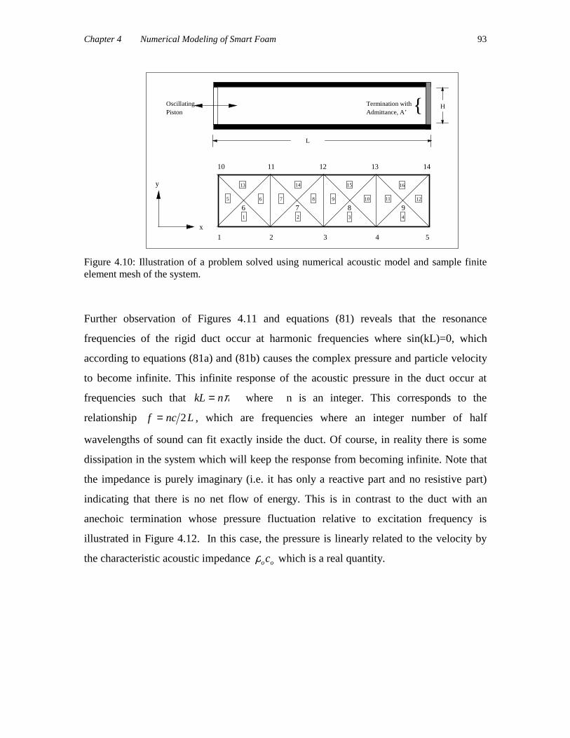
column is shown in Figure 4.10 and indicates the node and element numbering scheme.
The element numbers are the described by the boxed numbers and the nodal numbers are
not boxed. Figures 4.11 and Figure 4.12 shows the results for a duct having a rigid
termination and anechoic termination. Excellent agreement is obtained in each case. To
achieve less than 1.0% error within the 0<f<2000 Hz frequency range, the numerical
model used 25 elements in the horizontal direction (number of horizontal elements
0<x<L and y=0). Consequently, the accuracy of the acoustic finite element model is
verified.
Chapter 4 Numerical Modeling of Smart Foam 93
1 2 3 4 5
6 7 8 9
10 11 12 13 14
1 2 3 4
5 6 7 8 9 10 11 12
13 14 15 16
x
y
Oscillating Piston
Termination withAdmittance, A’
L
H
Figure 4.10: Illustration of a problem solved using numerical acoustic model and sample finiteelement mesh of the system.
Further observation of Figures 4.11 and equations (81) reveals that the resonance
frequencies of the rigid duct occur at harmonic frequencies where sin(kL)=0, which
according to equations (81a) and (81b) causes the complex pressure and particle velocity
to become infinite. This infinite response of the acoustic pressure in the duct occur at
frequencies such that kL n= π where n is an integer. This corresponds to the
relationship f nc L= 2 , which are frequencies where an integer number of half
wavelengths of sound can fit exactly inside the duct. Of course, in reality there is some
dissipation in the system which will keep the response from becoming infinite. Note that
the impedance is purely imaginary (i.e. it has only a reactive part and no resistive part)
indicating that there is no net flow of energy. This is in contrast to the duct with an
anechoic termination whose pressure fluctuation relative to excitation frequency is
illustrated in Figure 4.12. In this case, the pressure is linearly related to the velocity by
the characteristic acoustic impedance ρo oc which is a real quantity.

Chapter 4 Numerical Modeling of Smart Foam 94
0 200 400 600 800 1000 1200 1400 1600 1800 2000100
110
120
130
140
150
160
170
180(a)
Analytical @ x=0 FEM @ x=0
SPL
(dB
)
Frequency (Hz)
0 200 400 600 800 1000 1200 1400 1600 1800 2000140
145
150
155
160
165
170
175
180
185(b)
Analytical @ x=L FEM @ x=L
SPL
(dB
)
Frequency (Hz)
Figure 4.11: Verification of FEM model of acoustic system. Average SPL at x=0 and x=L vs.frequency for rigid air-filled duct excited by an oscillating piston.

Chapter 4 Numerical Modeling of Smart Foam 95
0 200 400 600 800 1000 1200 1400 1600 1800 2000142.0
142.5
143.0
143.5
144.0
144.5
145.0
Analytical @ x=0, x=L FEM @ x=0, x=L
SPL
(dB
)
Frequency (Hz)
Figure 4.12: Verification of FEM model of acoustic system. Average SPL at x=0 and x=L vs.frequency for rigid air-filled duct with anechoic termination excited by an oscillating piston.
4.11 Finite Element Formulation of Piezoelectric Actuator
The piezoelectric effect is the coupled interaction between structural deformation
and electrical fields in a material. Applying electrical fields to a piezoelectric material
causes the material to strain and, conversely, applying mechanical strains causes electric
fields to be generated in the piezoelectric material. In smart foam noise control
applications, an electrical field is applied to the embedded piezoelectric actuator, known
as PVDF, which is embedded in acoustic foam. To perform finite element analysis
involving piezoelectric effects, coupled field elements which take into account structural
and electrical coupling is needed. The PVDF actuator may be considered as an axial
member of length L which experiences in-plane deformation as shown in Figure 4.13(a).
Note that the element has one degree of freedom per node since only horizontal
displacement is allowed. Figure 4.13(b) illustrates the same element but uses two degrees
of freedom per node to do so. This is due to the change in orientation of the element as it
is rotated by an angle, β , resulting in horizontal and vertical displacements at each node.

Chapter 4 Numerical Modeling of Smart Foam 96
y, v
x, u
y’, v’
x’, u’
L
y, v
x, u
y’, v’x’, u’
L
Node 1 Node 2 Node 1
Node 2
(a) (b)
β
(c) y, v
x, uR
1
2
3
12
4
56 7
8
9
10
11
β=15 oθ
Figure 4.13(a): Piezoelectric finite element with one degree of freedom per node (b) Piezoelectricfinite element with two degrees of freedom per node (c) Assembly of piezoelectric finiteelements to establish cylindrical actuator of radius, R.
The kinetic energy density associated with axial deformation of the actuator is
described by
dT m uL=•1
2
2
(81)
where mL is the mass per unit length of the actuator and u•
denotes the axial velocity. The
strain energy is expressed as
( )
dV d E
Ydu
dxY
du
dxd E
= +
=
+
1
2
1
2
1
2
1
2
31
2
31
σε σ (82)
where the symbol Y is the young’s modulus of the material, d31 is the piezoelectric strain
constant, and E is the applied field represented by the ratio of the excitation voltage to the
piezoelectric material thickness [29, 78]. The first term of the potential energy
expression defined in equation (82) is associated with the mechanical strain and the
Chapter 4 Numerical Modeling of Smart Foam 97
second term accounts for the piezoelectric effect. It will be seen that the second term is
related to the forcing function of the system.
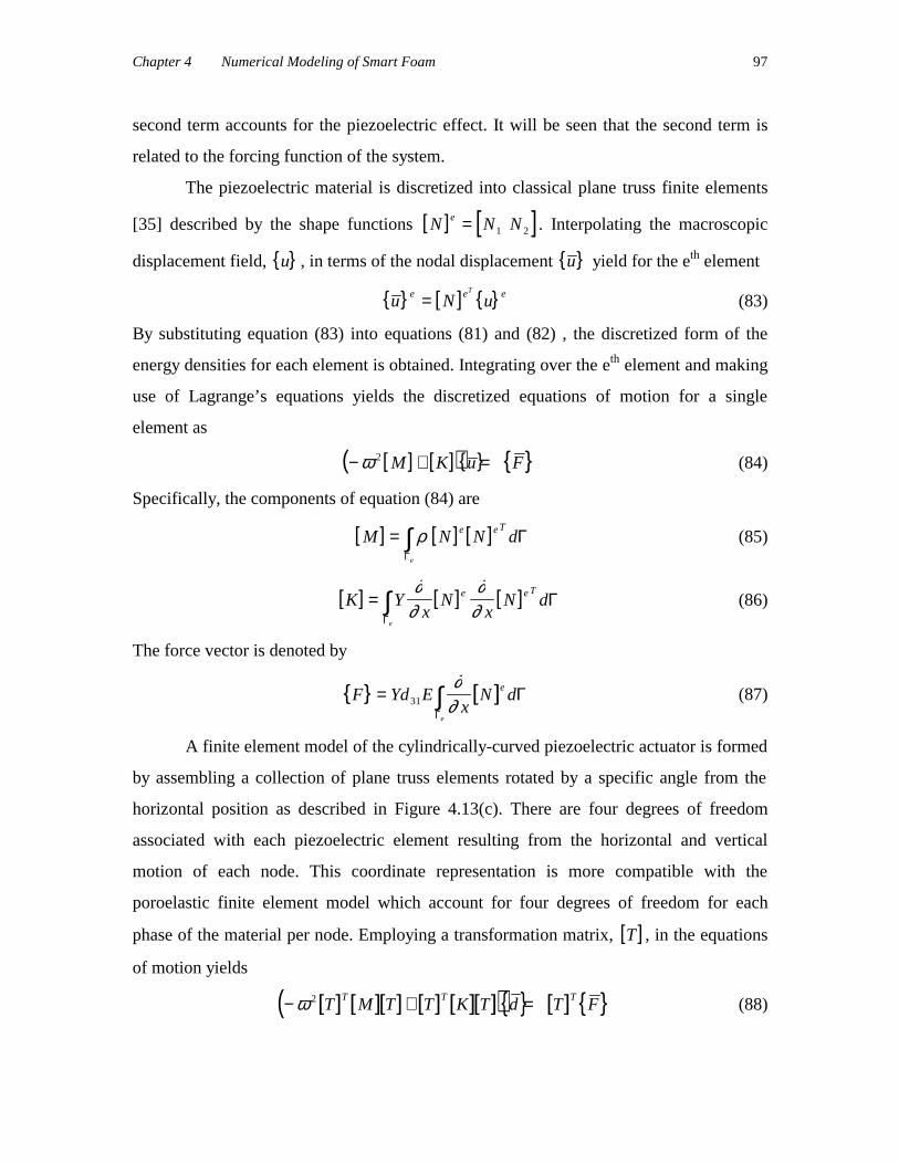
The piezoelectric material is discretized into classical plane truss finite elements
[35] described by the shape functions [ ] [ ]N N Ne = 1 2 . Interpolating the macroscopic
displacement field, u , in terms of the nodal displacement u yield for the eth element
[ ] u N ue e eT
= (83)
By substituting equation (83) into equations (81) and (82) , the discretized form of the
energy densities for each element is obtained. Integrating over the eth element and making
use of Lagrange’s equations yields the discretized equations of motion for a single
element as
[ ] [ ]( ) − + =ω 2 M K u F (84)
Specifically, the components of equation (84) are
[ ] [ ] [ ]M N N de e T
e
= ∫ ρ ΓΓ
(85)
[ ] [ ] [ ]K Yx
Nx
N de e T
e
= ∫∂
∂∂
∂ ΓΓ
(86)
The force vector is denoted by
[ ]F Yd Ex
N de
e
= ∫31
∂∂
ΓΓ
(87)
A finite element model of the cylindrically-curved piezoelectric actuator is formed
by assembling a collection of plane truss elements rotated by a specific angle from the
horizontal position as described in Figure 4.13(c). There are four degrees of freedom
associated with each piezoelectric element resulting from the horizontal and vertical
motion of each node. This coordinate representation is more compatible with the
poroelastic finite element model which account for four degrees of freedom for each
phase of the material per node. Employing a transformation matrix, [ ]T , in the equations
of motion yields
[ ] [ ][ ] [ ] [ ][ ]( ) [ ] − + =ω 2 T M T T K T d T FT T T (88)

Chapter 4 Numerical Modeling of Smart Foam 98
where d u v u v= 1 1 2 2 and accounts for the horizontal and vertical motion of each
node as illustrated in Figure 4.14(b). The transformation matrix is defined as
T =
cos sin
cos sin
β ββ β
0 0
0 0 (89)
The global system representing the piezoelectric material is formulated by summing the
contribution of all elements in the domain.
The established piezoelectric finite element model can now be used to simulate
the vibrational response of a cylindrically-curved PVDF actuators as illustrated in Figure
4.13(c). Recall that the properties of the piezoelectric material used in this investigation
are given in section 2.2. The following simulations establish the horizontal and vertical
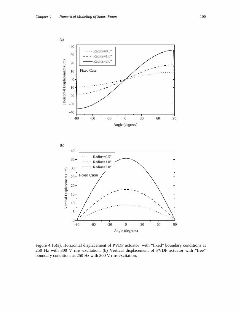
deflection of a PVDF actuator as the radius, R, is changed. Each actuator is excited with a
300 Vrms electrical input at 250 Hz. Figures 4.14 show the horizontal and vertical
displacement over the range − ≤ ≤90 90o oθ of three cylindrically-curved actuators of
0.5 inch, 1.0 inch and 2.0 inch radii, respectively. No constraints are enforced on the
actuator boundaries and this is considered the “Free Case”. These plots show that the
horizontal and vertical displacement amplitudes increase as the radius of the actuator
increases. A similar trend is observed in Figures 4.15 which represent the “Fixed Case”
and enforces zero displacement at θ = −90o and θ = 90o . Note that the actuator
displacement converges to a steady state solution when approximately 10 elements per
radial inch are used. This trend is valid up to an input frequency of 1000 Hz, which is the
frequency range in which active control is performed during future experiments.

Chapter 4 Numerical Modeling of Smart Foam 99
-90 -60 -30 0 30 60 90
-20
-10
0
10
20
(a)
Free Case
Radius=0.5" Radius=1.0" Radius=2.0"
Hor
izon
tal D
ispl
acem
ent (
υm)
Angle (degrees)
-90 -75 -60 -45 -30 -15 0 15 30 45 60 75 90
-20
-10
0
10
20
30
40
(b)
Free Case
Radius=0.5" Radius=1.0" Radius=2.0"
Ver
tical
Dis
plac
emen
t (υm
)
Angle (Degrees)
Figure 4.14(a): Horizontal displacement of PVDF actuator with “free” boundary conditions at250 Hz with 300 V rms excitation. (b) Vertical displacement of PVDF actuator with “fixed”boundary conditions at 250 Hz with 300 V rms excitation.
Chapter 4 Numerical Modeling of Smart Foam 100
-90 -60 -30 0 30 60 90
-40
-30
-20
-10
0
10
20
30
40
(a)
Fixed Case
Radius=0.5" Radius=1.0" Radius=2.0"
Hor
izon
tal D
ispl
acem
ent (
υm)
Angle (degrees)
-90 -60 -30 0 30 60 900
5
10
15
20
25
30
35
40
(b)
Fixed Case
Radius=0.5" Radius=1.0" Radius=2.0"
Ver
tical
Dis
plac
emen
t (υm
)
Angle (degrees)
Figure 4.15(a): Horizontal displacement of PVDF actuator with “fixed” boundary conditions at250 Hz with 300 V rms excitation. (b) Vertical displacement of PVDF actuator with “free”boundary conditions at 250 Hz with 300 V rms excitation.

Chapter 4 Numerical Modeling of Smart Foam 101
The presented results concerning the numerical modeling of cylindrically-curved PVDF
reveal that a fixed actuator exhibits the highest vertical displacement. With regard to
radius, it is shown that the displacement of the actuator increases as the radius of the
actuator increases. Figure 4.16 illustrates the average vertical displacement (in dB relative
to 1 µm ) for various cylindrically curved actuators. Each actuator has fixed end
conditions and the input voltage is 300 Vrms . In Figure 4.16, the displacement is plotted
as a function of frequency for an actuator with a 0.5, 1.0 and 2.0 inch radius. The results
show that the resonance frequency denoted by the peak in each curve is in the very high
frequency range (i.e. above 100 MHz). The frequency range of interest in this study is
well below the first resonance frequency exhibited by each actuator. It is observed that in
the low frequency region (i.e. below the first resonance), the larger actuator exhibits the
highest displacement. Since the actuator displacement is directly proportional to sound
output, the largest PVDF actuator is identified as the most acoustically efficient.
0 100 200 300 400 5000
5
10
15
20
25
30
35
40
Fixed Case Radius=0.5" Radius=1.0" Radius=2.0"
Ave
rage
Ver
tical
Dis
plac
emen
t (dB
rel
1 u
m)
Frequency (MHz)
Figure 4.16: Average vertical displacement of PVDF actuator with “fixed” boundary conditionsvs. frequency with 300 V rms excitation.

Chapter 4 Numerical Modeling of Smart Foam 102
4.12 Coupling of Poroelastic Finite Elements with Acoustic Finite Element
In the development of a smart foam finite element formulation, the coupling
conditions at the nodal points adjoining the different material interfaces must be enforced.
The boundary conditions between the absorptive foam system, recognizing its’ dual solid
and fluid phases, and the acoustic system are
− =
− − =
=
= − +
φ σφ σ
σω φ ωφ
p
p
v j u j U
xf
xs
xys
x x x
( )
( )
1
0
1
(90)
Note that vx denotes the velocity of the air in the acoustic system at the foam surface. The
first two conditions of equation (90) enforce compatibility of normal forces in the air-
fluid and air-solid interfaces, respectively. The third condition ensures that the shear force
is equal to zero on the solid surface of the foam due to the assumed normal incident
acoustic wave excitation. The fourth condition satisfies continuity of normal volume
velocity at the interface.
Before establishing the coupled finite element formulation describing the
poroelastic-acoustic system, some modification of the independent equations of motion
for each subdomain must be made. Comparing equations (73) and (80), it is observed that
the force vectors of the poroelastic and acoustic systems are expressed in different
physical forms. The force vector is expressed in terms of forces for the poroelastic system
while the force vector is expressed in terms of volume flow rates for the acoustic system.
This mismatch arises because it is convenient to express the solution vector in terms of
displacements for the foam system while the solution vector of the acoustic system is
easily described in terms of acoustic pressure. Accordingly, it is necessary to collocate
two nodes at the poroelastic-acoustic interface. One node is a component of the
poroelastic finite element and the other node belongs to the acoustic finite element,
allowing a decoupling of the two systems. The two subdomains are then coupled by
enforcing the boundary conditions (90) in equations (73) and (80) to yield

Chapter 4 Numerical Modeling of Smart Foam 103
F p N N d
F
F p N N d
F
Q u N N d U N N d
i jj
m
i j
i
i jj
m
i j
i
i o j i jj
m
o j i jj
m
e
e
e e
1
1
2
3
1
4
2
1
2
1
1
0
0
1
≈ −
=
=
=
≈ − +
=
=
= =
∑ ∫
∑ ∫
∫∑ ∫∑
( )
( )
φ
φ
ω ρ φ ω ρ φ
Γ
Γ
Γ Γ
Γ
Γ
Γ Γ
(91)
The force vector of the poroelastic system is now described in terms of acoustic pressure
and the force vector of the acoustic system is now described in terms of the displacements
of the solid and fluid phases of the foam at the interface. As a result, the global finite
element formulation of the poroelastic-acoustic system is denoted by
[ ] [ ]
[ ] [ ]
K K
K K
p
u
v
U
V
Q
F
F
F
F
a af
afT
f
=
1
2
3
4
(92)
where the matrices [ ]Ka and [ ]Kf are the dynamic stiffness matrices for the independent
acoustic and foam systems, respectively. The matrices [ ]Kaf and [ ]KafT denotes the
coupling between the acoustic and poroelastic subdomains and its’ transpose,
respectively. The sub-vector Q on the right side accounts for any applied acoustic
velocities. The sub-vectors F1 and F 2 include any externally applied forces acting
on the solid phase in the x and y directions, respectively. The sub-vectors F 3 and
F 4 include any externally applied forces acting on the solid phase in the x and y
directions, respectively.
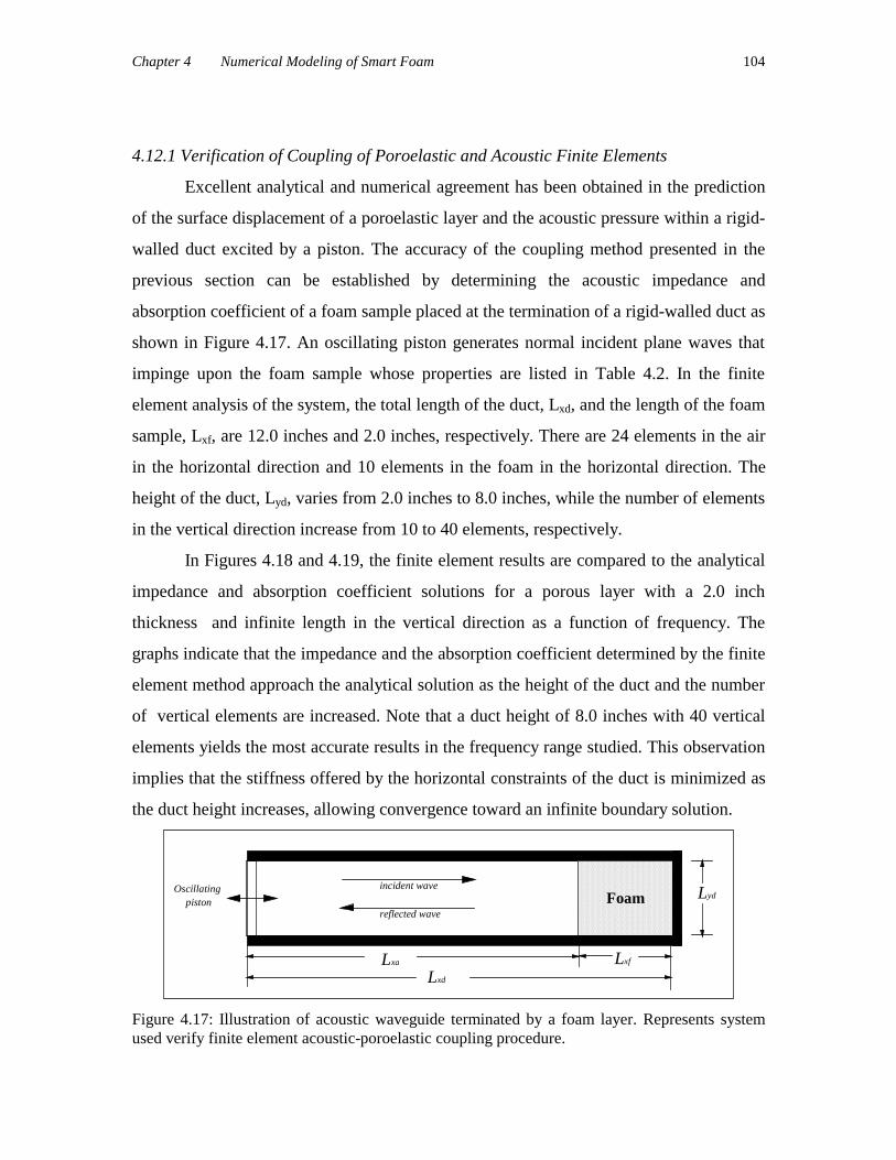
Chapter 4 Numerical Modeling of Smart Foam 104
4.12.1 Verification of Coupling of Poroelastic and Acoustic Finite Elements
Excellent analytical and numerical agreement has been obtained in the prediction
of the surface displacement of a poroelastic layer and the acoustic pressure within a rigid-
walled duct excited by a piston. The accuracy of the coupling method presented in the
previous section can be established by determining the acoustic impedance and
absorption coefficient of a foam sample placed at the termination of a rigid-walled duct as
shown in Figure 4.17. An oscillating piston generates normal incident plane waves that
impinge upon the foam sample whose properties are listed in Table 4.2. In the finite
element analysis of the system, the total length of the duct, Lxd, and the length of the foam
sample, Lxf, are 12.0 inches and 2.0 inches, respectively. There are 24 elements in the air
in the horizontal direction and 10 elements in the foam in the horizontal direction. The
height of the duct, Lyd, varies from 2.0 inches to 8.0 inches, while the number of elements
in the vertical direction increase from 10 to 40 elements, respectively.
In Figures 4.18 and 4.19, the finite element results are compared to the analytical
impedance and absorption coefficient solutions for a porous layer with a 2.0 inch
thickness and infinite length in the vertical direction as a function of frequency. The
graphs indicate that the impedance and the absorption coefficient determined by the finite
element method approach the analytical solution as the height of the duct and the number
of vertical elements are increased. Note that a duct height of 8.0 inches with 40 vertical
elements yields the most accurate results in the frequency range studied. This observation
implies that the stiffness offered by the horizontal constraints of the duct is minimized as
the duct height increases, allowing convergence toward an infinite boundary solution.
Oscillating piston
incident wave
reflected waveFoam
Lxa Lxf
Lxd
Lyd
Figure 4.17: Illustration of acoustic waveguide terminated by a foam layer. Represents systemused verify finite element acoustic-poroelastic coupling procedure.

Chapter 4 Numerical Modeling of Smart Foam 105
200 400 600 800 1000 1200 1400 1600 1800 20001.0
1.5
2.0
2.5
3.0
3.5
4.0
4.5
5.0
5.5
6.0
6.5
7.0(a)
Analytical Size (x,y)=(2.0"x2.0"), # of elements=(10x10) Size (x,y)=(2.0"x4.0"), # of elements=(10x20) Size (x,y)=(2.0"x8.0"), # of elements=(10x40)
Rea
l(Z
/Zo)
Frequency (Hz)
200 400 600 800 1000 1200 1400 1600 1800 2000-4
-3
-2
-1
0
1
2
3
4
5
6
7(b)
Analytical Size (x,y)=(2.0"x2.0"), # of elements=(10x10) Size (x,y)=(2.0"x4.0"), # of elements=(10x20) Size (x,y)=(2.0"x8.0"), # of elements=(10x40)
Imag
(Z/Z
o)
Frequency (Hz)
Figure 4.18: Comparison of normalized acoustic impedance as determined by analytical andfinite element methods (a) Real part. (b) Imaginary part.
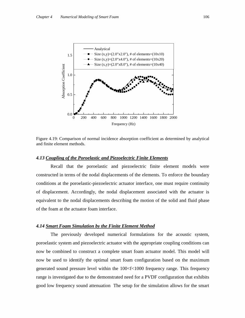
Chapter 4 Numerical Modeling of Smart Foam 106
0 200 400 600 800 1000 1200 1400 1600 1800 20000.0
0.5
1.0
1.5
Analytical Size (x,y)=(2.0"x2.0"), # of elements=(10x10) Size (x,y)=(2.0"x4.0"), # of elements=(10x20) Size (x,y)=(2.0"x8.0"), # of elements=(10x40)
Abs
orpt
ion
Coe
ffic
ient
Frequency (Hz)
Figure 4.19: Comparison of normal incidence absorption coefficient as determined by analyticaland finite element methods.
4.13 Coupling of the Poroelastic and Piezoelectric Finite Elements
Recall that the poroelastic and piezoelectric finite element models were
constructed in terms of the nodal displacements of the elements. To enforce the boundary
conditions at the poroelastic-piezoelectric actuator interface, one must require continuity
of displacement. Accordingly, the nodal displacement associated with the actuator is
equivalent to the nodal displacements describing the motion of the solid and fluid phase
of the foam at the actuator foam interface.
4.14 Smart Foam Simulation by the Finite Element Method
The previously developed numerical formulations for the acoustic system,
poroelastic system and piezoelectric actuator with the appropriate coupling conditions can
now be combined to construct a complete smart foam actuator model. This model will
now be used to identify the optimal smart foam configuration based on the maximum
generated sound pressure level within the 100<f<1000 frequency range. This frequency
range is investigated due to the demonstrated need for a PVDF configuration that exhibits
good low frequency sound attenuation The setup for the simulation allows for the smart

Chapter 4 Numerical Modeling of Smart Foam 107
foam actuator to be positioned within one end of a rigid duct that has an anechoic
termination at the opposite end as shown in Figure 4.20. As stated earlier, the primary
requirement for the smart foam to radiate sound is to contain a piezoelectric actuator that
is physically curved in order to translate in-plane strain to out-of-plane motion with an
applied voltage. With regard to this requirement, the sound output generated by
“triangular” and “cylindrically” shaped actuators are studied. The height of the rigid duct
and each smart foam array is 41.0 cm (16.0 inches) and the length of the air within the
duct is approximately 1.0 m. The length of the smart foam array varies depending on
the embedded PVDF configuration. A total of six unique smart foam configurations are
investigated and each differ in physical orientation, wavelength, thickness and boundary
conditions, as illustrated in Figure 4.20 and described below:
(1) Four free triangles: Array dimension (x,y)=(2.0 inches, 16.0 inch). PVDF actuatorshaped as a series of four triangles with free rear boundary conditions.
(2) Four free half-cylinders: Array dimension (x,y)=(2.0 inches, 16.0 inch). PVDFactuator shaped as a series of four half-cylinders with free rear boundary conditions.
(3) Eight free triangles: Array dimension (x,y)=(1.0 inches, 16.0 inch). PVDF actuatorshaped as a series of eight triangles with free rear boundary conditions.
(4) Eight free half-cylinders: Array dimension (x,y)=(1.0 inches, 16.0 inch). PVDFactuator shaped as a series of eight half-cylinders with free rear boundary conditions.
(5) Four fixed triangles: Array dimension (x,y)=(2.0 inches, 16.0 inch). PVDF actuatorshaped as a series of four triangles with fixed rear boundary conditions.
(6) Four fixed half-cylinders: Array dimension (x,y)=(2.0 inches, 16.0 inch). PVDFactuator shaped as a series of four half-cylinders with fixed rear boundary conditions
(7) Eight fixed triangles: Array dimension (x,y)=(1.0 inches, 16.0 inch). PVDF actuatorshaped as a series o eight triangles with fixed rear boundary conditions.
(8) Eight fixed half-cylinders: Array dimension (x,y)=(1.0 inches, 16.0 inch). PVDFactuator shaped as a series of eight half-cylinders with fixed rear boundary conditions
Figures 4.21 illustrates the sound pressure levels generated by each configuration
at the anechoic termination. The responses of smart foam with various embedded PVDF
actuators shaped as half-cylinders are presented in Figure 4.21(a). Similarly, the
responses of smart foam with various embedded PVDF actuators configured as triangles
are illustrated in Figure 4.19(b). In general, the primary observation seen in both figures is

Chapter 4 Numerical Modeling of Smart Foam 108
that the sound generation of each smart foam configuration studied increases as the
frequency of excitation increases. In Figure 4.21(a), it is further evident that the smart
foam with cylindrically curved actuators having fixed boundary condition at the rear
surface is the optimal configuration because it is the most acoustically efficient. By
comparing the smart foam configured with four and eight half-cylinders, both having
fixed boundary conditions, it is evident that the actuator with four half cylinders is the
most efficient. These results confirm that for low frequency sound generation, as the size
or wavelength of the embedded PVDF actuators increases an increase in sound output is
yielded. Referring to Figure 4.21(a), a comparison of the response given by the
cylindrically curved actuators with free boundary conditions at the rear surface indicates
that below 400 Hz, they are capable of yielding comparable sound output as the fixed
actuator cases. Above 400 Hz, it is revealed that as the size or wavelength of the free
PVDF actuators is increased, they are capable of generating a higher sound output.
However, in the studied frequency range, the smart foam with four embedded half-
cylinders with fixed boundary conditions offers superior performance. Similar trends are
noted in Figure 4.21(b), which reveal the response of various smart foam actuators
configured with a series of embedded PVDF shaped as triangles. In comparison to the
cylindrically-curved actuators, the triangular actuators are not as efficient. In summary,
the smart foam actuators manufactured in Chapter 5 for the duct noise control
experiments will contain cylindrically-curved PVDF with fixed boundary conditions. The
radius of each actuator will be limited by the power amplifier specifications and the area
of the commercially available PVDF film, but it is intended to allow the embedded PVDF
to have the largest radius possible within the smart foam.

Chapter 4 Numerical Modeling of Smart Foam 109
SmartFoamArray
Anechoic
Term
inationPropagating sound waves
Lyf
LxfLxa
1 2 3 4 5 6 7 8
Various Smart Foam Array configurations studied in numerical analysis
Figure 4.20 Illustration of smart foam actuator configurations investigated using the finiteelement approach : Smart foam with embedded PVDF shaped as (1) Four free triangles, (2) Fourfree half-cylinders (3) Eight free triangles, (4) Eight free half-cylinders, (5) Four fixed triangles,(6) Four fixed half-cylinders, (7) Eight fixed triangles, and (8) Eight fixed half-cylinders.
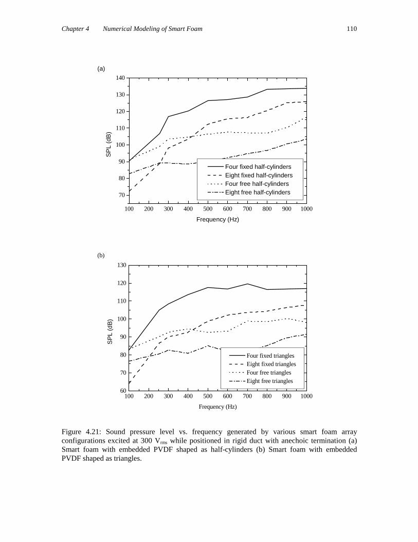
Chapter 4 Numerical Modeling of Smart Foam 110
100 200 300 400 500 600 700 800 900 1000
70
80
90
100
110
120
130
140
(a)
Four fixed half-cylinders Eight fixed half-cylinders Four free half-cylinders Eight free half-cylinders
SP
L (d
B)
Frequency (Hz)
100 200 300 400 500 600 700 800 900 100060
70
80
90
100
110
120
130
(b)
Four fixed triangles Eight fixed triangles Four free triangles Eight free triangles
SP
L (d
B)
Frequency (Hz)
Figure 4.21: Sound pressure level vs. frequency generated by various smart foam arrayconfigurations excited at 300 Vrms while positioned in rigid duct with anechoic termination (a)Smart foam with embedded PVDF shaped as half-cylinders (b) Smart foam with embeddedPVDF shaped as triangles.
Chapter 4 Numerical Modeling of Smart Foam 111
4.15 Summary
A numerical formulation of the composite smart foam actuator was established in
this chapter. The composite operates in an acoustic environment and requires proper
modeling of porous materials, acoustic and piezoelectric systems.
Prior to presenting the numerical smart foam simulations, the analytical Biot
theory for the modeling of a porous sound absorbing acoustic foam used in this study was
presented. It revealed the unique characteristics of the dual-phase foam used in noise
control applications relative to homogeneous elastic materials in that:
(1) the wavepeed of the compressional wave associated with the frame, P1, is the fastestof the three wavetypes and is virtually independent of frequency.
(2) the compressional wave associated with the fluid, P2, has the highest attenuation perwavelength up to 40000 Hz and provides the bulk of the acoustic energy dissipation ofthe three wavetypes.
(3) the shear wave, P3,, travels only in the solid phase of the foam.
(4) the presence of the fluid in the pores of the material increases the stiffness of the bulkmaterial.
(5) compared to an equivalent rigid porous material, the finite frame elasticity has theeffect of reducing the phase velocity of the airborne wave.
A numerical foam model using linear triangular elements was established and comparison
of the foam displacement generated by a mechanical force showed excellent agreement
with the Biot model predictions. Linear triangular elements were implemented to
formulate an acoustic numerical model of an air-filled rigid duct excited by an oscillating
piston. Excellent agreement was obtained when the pressure within the duct was
compared to that predicted by the analytical solution. A piezoelectric numerical model
was constructed using simple axial elements and verified by published analytical
solutions on curved piezoelectric actuators. Once the numerical modeling of the acoustic
foam, air and piezoelectric material was completed and verified with analytical solutions,
a smart foam code programmed in MATLAB® by the author allowed investigation of the
acoustic response of either “cylindrical or triangular” shaped piezoelectric actuators

Chapter 4 Numerical Modeling of Smart Foam 112
embedded within the foam to identify the optimal configuration for low frequency sound
control. It was determined that a series of cylindrically curved PVDF actuators with fixed
boundary conditions offered the highest low frequency sound output. It is further evident
that the radius of the embedded PVDF actuators should be as large as the physical
constraints imposed by the finite thickness of the foam will permit.