Embed Size (px)
Citation preview
RESEARCH ARTICLE
J.Natn.Sci.Foundation Sri Lanka 2019 47 (4): 421 - 433 DOI: http://dx.doi.org/10.4038/jnsfsr.v47i4.9679
Numerical modelling of the spatial variation of sediment transport using wave climate schematisation method - a case study of west coast of Sri Lanka
Submitted: 10 January 2019; Revised: 17 July 2019; Accepted: 26 July 2019
08.2018
* Corresponding author ([email protected] ; https://orcid.org/0000-0002-1105-8764)
This article is published under the Creative Commons CC-BY-ND License (http://creativecommons.org/licenses/by-nd/4.0/). This license permits use, distribution and reproduction, commercial and non-commercial, provided that the original work is properly cited and is not changed in anyway.
INTRODUCTION
The ever-increasing economic and environmental considerations of coastal zones have provoked further studies of the variety of coastal processes such as coastal erosion, deposition and sediment transportation. Development within the coastal areas has increased interest in management of coastal erosion and restoration of coastal capacity to accommodate short- and long-term changes induced by human activities, extreme events and sea level rise. Coastal erosion problem becomes worse whenever the countermeasures (i.e. hard or soft structural options) are inappropriately applied, improperly designed, built, or maintained and if the effects on adjacent shores are not carefully evaluated. Often erosion is addressed locally at specific places or at regional or jurisdictional boundaries instead of at system boundaries that reflect natural processes. Human activities along the coast (land reclamation, port development, shrimp farming) and offshore (dredging, sand mining) in combination with these natural forces often exacerbate coastal erosion in many places and jeopardise opportunities for the coasts to fulfil their socio-economic and ecological roles in the long term at a reasonable societal cost. Moreover, the Western and Southern provinces are linked by two of the country’s busiest highways and railway lines, touching the coast along most of their length (Garcin et al., 2008).
Abstract: This study quantifies the variations in wave characteristics and the resulting variations in potential longshore sediment transport rate along the coastline between Mount Lavinia and Negombo, Sri Lanka. Over the last 25 years, this coastal belt has been subjected to dramatic interventions due to the influence of rapid socio-economic development in the country such as construction of the Colombo South Harbor jetty, ongoing Colombo Port City Project and mega sand dreading off Negombo coast. For the wave transformation, SWAN (Simulating Waves Nearshore) numerical model was applied, forced by offshore wave/wind. The Delft3D-FLOW model was used to estimate the longshore sediment transport rates and related morphodynamics using input reduction and morphological acceleration techniques. Results of the alongshore sediment transport capacity computations clearly indicate the variable characteristics of different parts of the study zone. The annual alongshore sediment transport capacity computed in the study area oriented northward, complying very well with the observations. The coastal belt between Mount Lavinia and Colombo, the wave climate, and subsequently the annual alongshore transport reached the highest values indicating a relative dynamic environment and thereafter decreased with a strong gradient northward. The explanation for these negative steep gradients and the environmental forcing/human interventions that govern the regional sediment transport are discussed in this paper.
Keywords: ERA Interim, morphodynamics, morphological acceleration, sediment transport, SWAN.
R.M.R.M. Jayathilaka1* and M.C.S. Fernando21 National Aquatic Resources Research and Development Agency, Crow Island, Colombo 15.2 Department of Mathematics, Faculty of Science, University of Ruhuna, Matara.
422 R.M.R.M. Jayathilaka & M.C.S. Fernando
December 2019 Journal of the National Science Foundation of Sri Lanka 47(4)
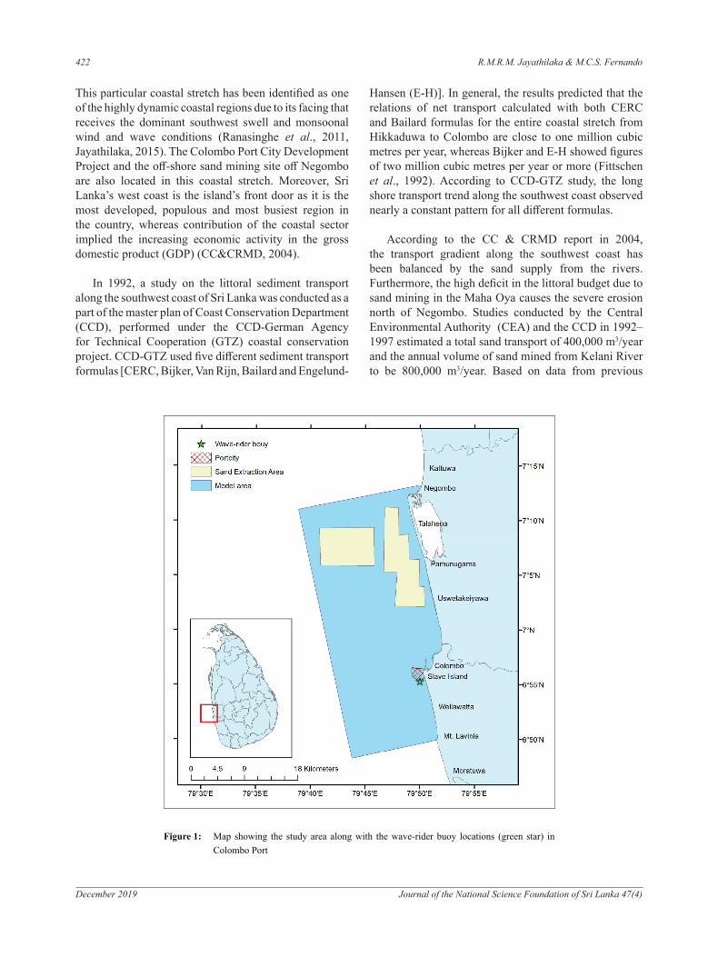
This particular coastal stretch has been identified as one of the highly dynamic coastal regions due to its facing that receives the dominant southwest swell and monsoonal wind and wave conditions (Ranasinghe et al., 2011, Jayathilaka, 2015). The Colombo Port City Development Project and the off-shore sand mining site off Negombo are also located in this coastal stretch. Moreover, Sri Lanka’s west coast is the island’s front door as it is the most developed, populous and most busiest region in the country, whereas contribution of the coastal sector implied the increasing economic activity in the gross domestic product (GDP) (CC&CRMD, 2004).
In 1992, a study on the littoral sediment transport along the southwest coast of Sri Lanka was conducted as a part of the master plan of Coast Conservation Department (CCD), performed under the CCD-German Agency for Technical Cooperation (GTZ) coastal conservation project. CCD-GTZ used five different sediment transport formulas [CERC, Bijker, Van Rijn, Bailard and Engelund-
Hansen (E-H)]. In general, the results predicted that the relations of net transport calculated with both CERC and Bailard formulas for the entire coastal stretch from Hikkaduwa to Colombo are close to one million cubic metres per year, whereas Bijker and E-H showed figures of two million cubic metres per year or more (Fittschen et al., 1992). According to CCD-GTZ study, the long shore transport trend along the southwest coast observed nearly a constant pattern for all different formulas.
According to the CC & CRMD report in 2004, the transport gradient along the southwest coast has been balanced by the sand supply from the rivers. Furthermore, the high deficit in the littoral budget due to sand mining in the Maha Oya causes the severe erosion north of Negombo. Studies conducted by the Central Environmental Authority (CEA) and the CCD in 1992–1997 estimated a total sand transport of 400,000 m3/year and the annual volume of sand mined from Kelani River to be 800,000 m3/year. Based on data from previous
Fig. 1. Map showing the study area along with the wave-rider buoy locations ( green star) in Colombo Port.
2. Methodology
2.1. Model description and settings
Numerical simulations were carried out by means of the process based model Delft3D to obtain state-
of-the-art estimates of the annual longshore sediment transport rates. The DelftD software is
developed by Deltares, The Netherlands is a world leading 3D modelling suite to investigate
Figure 1: Map showing the study area along with the wave-rider buoy locations (green star) in Colombo Port
Sediment transport - West coast of Sri Lanka 423
Journal of the National Science Foundation of Sri Lanka 47(4) December 2019
studies on sand supply to the coast and the Coastal Resources Management Project-1999, the estimated sand supply to the coast is 100,000 m3/year representing a significant decline. A study conducted in 1999 (CC & CRMD, 2004) estimated that the sediment outflow from the Kelani River would further decline by 40 % in the next 12 years. A study conducted by the University of Moratuwa, Sri Lanka (Ansaf, 2012) estimated coastal transport rates of the various coastal segments between Galle to Colombo using MIKE21 modelling (developed by the Danish Hydraulics Institute). The results of MIKE21 showed the northward net transport rate along the coastline from Galle to Colombo.
The main objectives of the present study were to (1) obtain a better understanding of near shore wave climate and (2) quantify the alongshore sediment transport rates along the west coast from Mount Lavinia to Negombo (Figure 1).
METHODOLOGY
Model description and settings
Numerical simulations were carried out by means of the process-based model Delft3D to obtain state-of-the-art estimates of the annual longshore sediment transport rates. The Delft3D software developed by the Deltares, Netherlands is a world leading 3D modelling suite to investigate hydrodynamics, sediment transport and morphology and water quality for fluvial, estuarine and coastal environments. The applications of Delft3D have proven its capabilities on many places around the world, like The Netherlands, USA, Hong Kong, Singapore, Australia, Venice, UAE, etc. In the context of Sri Lanka, Delft3D applications are hardly found except for a few collaboration studies of foreign experts (Jayathilaka, 2015; Duong et al., 2016).
Delft3D combines a short-wave driver (SWAN), a 2DH flow module, a sediment transport model (Van Rijn & Boer, 2006), and a bed level update scheme that solves the 2D sediment continuity equation (Hydraulics, 1999). In particular, the hydrodynamic and sediment transport module Delft3D-FLOW, and the wave module Delft3D-WAVE were used (Hydraulics, 2006; Lesser, 2009; Giardino et al., 2010). The Delft3D-FLOW and Delft3D-WAVE exchange information by means of online coupling.
We start from a bathymetry, given on a detailed two-dimensional grid (in case of area models) or one dimension
(in case of coastline or coastal profile models). Wave and current fields, which usually interact together, were predicted by the given boundary conditions for waves and currents, these processes determine the sediment transport. The sediment transport gradients lead to bottom changes, which then feedback into the bathymetry, the currents and waves and the sediment transports etc. Delft3D wave parameters and coefficients such as depth-induced breaking, non-linear triad interactions and bottom friction were applied and checked on the wave runs. Further, different processes such as wind and wave growth, white-capping, quadruplet’s interaction and refraction were activated and de-activated to understand their effect on the results of Delft3D.
Sediment transport formula
The sediment transport and morphology module of Delft3D supports both bed load and suspended load transport of non-cohesive sediments and suspended load of cohesive sediments (Lesser et al., 2004). Sediment transport algorithms, predominantly based on the formulations of Van Rijn (1993), were added to the Delft3D-FLOW hydrodynamic solver which is widely used, well tested, and well suited to modelling the three-dimensional hydrodynamics of coastal regions (Hydraulics, 2006). The settling velocity of a non-cohesive (‘sand’) sediment fraction was computed following the method of Van Rijn (1993).
The suspended load transport can be determined by depth-integration of the product of sand concentration and fluid velocity from the top of the bed load layer (at about 0.01 m above the bed) to the water surface. Herein, the net (averaged over the wave period) total sediment transport is obtained as the sum of net bed-load
Alpha: 0.1 Beta: 2.2
Refraction Bottom friction Activated Type: JONSWAP Coefficient: 0.2 (m2 s-3)
2.2. Sediment transport Formula
The sediment transport and morphology module of Delft3D supports both bed load and suspended
load transport of non-cohesive sediments and suspended load of cohesive sediments (Lesser et al.,
2004). Sediment transport algorithms, predominantly based on the formulations of Van Rijn (1993),
are added to the Delft3D-FLOW hydrodynamic solver which is widely used, well tested, and well
suited to modelling the three-dimensional hydrodynamics of coastal regions (Hydraulics, 2006). The
settling velocity of a non-cohesive (“sand”) sediment fraction is computed following the method of
Van Rijn (1993).
The suspended load transport can be determined by depth-integration of the product of sand
concentration and fluid velocity from the top of the bed load layer (at about 0.01 m above the bed) to
the water surface. Herein, the net (averaged over the wave period) total sediment transport is obtained
as the sum of net the bed load (q�) and net suspended load (q�) transport rates, as follows:
q��� = q� + q� (1)
The net bed-load transport rate in conditions with uniform bed material is obtained by time-averaging
(over the wave period T) of the instantaneous transport rate using a bed-load transport formula (quasi-
steady approach), as follows:
q� = ���� . ∫ q�,� dt (2)
q� = γ. ρ�. d��. D∗��.��τ́�,��/ρ�
�.��(τ� �,�� − τ�,��)/τ�,���
� (3)
in which, τ́�,��: instantaneous grain-related bed-shear stress due to both currents and waves τ́�,�� =
0.5 ρ f���(U�,��)�, U�,��: Instantaneous velocity due to currents and waves at edge of wave boundary
Commented [m12]: Not under Reference
Commented [m13]: Not under Reference
and net suspended load
Alpha: 0.1 Beta: 2.2
Refraction Bottom friction Activated Type: JONSWAP Coefficient: 0.2 (m2 s-3)
2.2. Sediment transport Formula
The sediment transport and morphology module of Delft3D supports both bed load and suspended
load transport of non-cohesive sediments and suspended load of cohesive sediments (Lesser et al.,
2004). Sediment transport algorithms, predominantly based on the formulations of Van Rijn (1993),
are added to the Delft3D-FLOW hydrodynamic solver which is widely used, well tested, and well
suited to modelling the three-dimensional hydrodynamics of coastal regions (Hydraulics, 2006). The
settling velocity of a non-cohesive (“sand”) sediment fraction is computed following the method of
Van Rijn (1993).
The suspended load transport can be determined by depth-integration of the product of sand
concentration and fluid velocity from the top of the bed load layer (at about 0.01 m above the bed) to
the water surface. Herein, the net (averaged over the wave period) total sediment transport is obtained
as the sum of net the bed load (q�) and net suspended load (q�) transport rates, as follows:
q��� = q� + q� (1)
The net bed-load transport rate in conditions with uniform bed material is obtained by time-averaging
(over the wave period T) of the instantaneous transport rate using a bed-load transport formula (quasi-
steady approach), as follows:
q� = ���� . ∫ q�,� dt (2)
q� = γ. ρ�. d��. D∗��.��τ́�,��/ρ�
�.��(τ� �,�� − τ�,��)/τ�,���
� (3)
in which, τ́�,��: instantaneous grain-related bed-shear stress due to both currents and waves τ́�,�� =
0.5 ρ f���(U�,��)�, U�,��: Instantaneous velocity due to currents and waves at edge of wave boundary
Commented [m12]: Not under Reference
Commented [m13]: Not under Reference
transport rates, as follows:
Alpha: 0.1 Beta: 2.2
Refraction Bottom friction Activated Type: JONSWAP Coefficient: 0.2 (m2 s-3)
2.2. Sediment transport Formula
The sediment transport and morphology module of Delft3D supports both bed load and suspended
load transport of non-cohesive sediments and suspended load of cohesive sediments (Lesser et al.,
2004). Sediment transport algorithms, predominantly based on the formulations of Van Rijn (1993),
are added to the Delft3D-FLOW hydrodynamic solver which is widely used, well tested, and well
suited to modelling the three-dimensional hydrodynamics of coastal regions (Hydraulics, 2006). The
settling velocity of a non-cohesive (“sand”) sediment fraction is computed following the method of
Van Rijn (1993).
The suspended load transport can be determined by depth-integration of the product of sand
concentration and fluid velocity from the top of the bed load layer (at about 0.01 m above the bed) to
the water surface. Herein, the net (averaged over the wave period) total sediment transport is obtained
as the sum of net the bed load (q�) and net suspended load (q�) transport rates, as follows:
q��� = q� + q� (1)
The net bed-load transport rate in conditions with uniform bed material is obtained by time-averaging
(over the wave period T) of the instantaneous transport rate using a bed-load transport formula (quasi-
steady approach), as follows:
q� = ���� . ∫ q�,� dt (2)
q� = γ. ρ�. d��. D∗��.��τ́�,��/ρ�
�.��(τ� �,�� − τ�,��)/τ�,���
� (3)
in which, τ́�,��: instantaneous grain-related bed-shear stress due to both currents and waves τ́�,�� =
0.5 ρ f���(U�,��)�, U�,��: Instantaneous velocity due to currents and waves at edge of wave boundary
Commented [m12]: Not under Reference
Commented [m13]: Not under Reference
...(1)
The net bed-load transport rate in conditions with uniform bed material was obtained by time-averaging (over the wave period T) of the instantaneous transport rate using a bed-load transport formula (quasi-steady approach), as follows:
Alpha: 0.1 Beta: 2.2
Refraction Bottom friction Activated Type: JONSWAP Coefficient: 0.2 (m2 s-3)
2.2. Sediment transport Formula
The sediment transport and morphology module of Delft3D supports both bed load and suspended
load transport of non-cohesive sediments and suspended load of cohesive sediments (Lesser et al.,
2004). Sediment transport algorithms, predominantly based on the formulations of Van Rijn (1993),
are added to the Delft3D-FLOW hydrodynamic solver which is widely used, well tested, and well
suited to modelling the three-dimensional hydrodynamics of coastal regions (Hydraulics, 2006). The
settling velocity of a non-cohesive (“sand”) sediment fraction is computed following the method of
Van Rijn (1993).
The suspended load transport can be determined by depth-integration of the product of sand
concentration and fluid velocity from the top of the bed load layer (at about 0.01 m above the bed) to
the water surface. Herein, the net (averaged over the wave period) total sediment transport is obtained
as the sum of net the bed load (q�) and net suspended load (q�) transport rates, as follows:
q��� = q� + q� (1)
The net bed-load transport rate in conditions with uniform bed material is obtained by time-averaging
(over the wave period T) of the instantaneous transport rate using a bed-load transport formula (quasi-
steady approach), as follows:
q� = ���� . ∫ q�,� dt (2)
q� = γ. ρ�. d��. D∗��.��τ́�,��/ρ�
�.��(τ� �,�� − τ�,��)/τ�,���
� (3)
in which, τ́�,��: instantaneous grain-related bed-shear stress due to both currents and waves τ́�,�� =
0.5 ρ f���(U�,��)�, U�,��: Instantaneous velocity due to currents and waves at edge of wave boundary
Commented [m12]: Not under Reference
Commented [m13]: Not under Reference
...(2)
Alpha: 0.1 Beta: 2.2
Refraction Bottom friction Activated Type: JONSWAP Coefficient: 0.2 (m2 s-3)
2.2. Sediment transport Formula
The sediment transport and morphology module of Delft3D supports both bed load and suspended
load transport of non-cohesive sediments and suspended load of cohesive sediments (Lesser et al.,
2004). Sediment transport algorithms, predominantly based on the formulations of Van Rijn (1993),
are added to the Delft3D-FLOW hydrodynamic solver which is widely used, well tested, and well
suited to modelling the three-dimensional hydrodynamics of coastal regions (Hydraulics, 2006). The
settling velocity of a non-cohesive (“sand”) sediment fraction is computed following the method of
Van Rijn (1993).
The suspended load transport can be determined by depth-integration of the product of sand
concentration and fluid velocity from the top of the bed load layer (at about 0.01 m above the bed) to
the water surface. Herein, the net (averaged over the wave period) total sediment transport is obtained
as the sum of net the bed load (q�) and net suspended load (q�) transport rates, as follows:
q��� = q� + q� (1)
The net bed-load transport rate in conditions with uniform bed material is obtained by time-averaging
(over the wave period T) of the instantaneous transport rate using a bed-load transport formula (quasi-
steady approach), as follows:
q� = ���� . ∫ q�,� dt (2)
q� = γ. ρ�. d��. D∗��.��τ́�,��/ρ�
�.��(τ� �,�� − τ�,��)/τ�,���
� (3)
in which, τ́�,��: instantaneous grain-related bed-shear stress due to both currents and waves τ́�,�� =
0.5 ρ f���(U�,��)�, U�,��: Instantaneous velocity due to currents and waves at edge of wave boundary
Commented [m12]: Not under Reference
Commented [m13]: Not under Reference
...(3)
424 R.M.R.M. Jayathilaka & M.C.S. Fernando
December 2019 Journal of the National Science Foundation of Sri Lanka 47(4)
in which,
Alpha: 0.1 Beta: 2.2
Refraction Bottom friction Activated Type: JONSWAP Coefficient: 0.2 (m2 s-3)
2.2. Sediment transport Formula
The sediment transport and morphology module of Delft3D supports both bed load and suspended
load transport of non-cohesive sediments and suspended load of cohesive sediments (Lesser et al.,
2004). Sediment transport algorithms, predominantly based on the formulations of Van Rijn (1993),
are added to the Delft3D-FLOW hydrodynamic solver which is widely used, well tested, and well
suited to modelling the three-dimensional hydrodynamics of coastal regions (Hydraulics, 2006). The
settling velocity of a non-cohesive (“sand”) sediment fraction is computed following the method of
Van Rijn (1993).
The suspended load transport can be determined by depth-integration of the product of sand
concentration and fluid velocity from the top of the bed load layer (at about 0.01 m above the bed) to
the water surface. Herein, the net (averaged over the wave period) total sediment transport is obtained
as the sum of net the bed load (q�) and net suspended load (q�) transport rates, as follows:
q��� = q� + q� (1)
The net bed-load transport rate in conditions with uniform bed material is obtained by time-averaging
(over the wave period T) of the instantaneous transport rate using a bed-load transport formula (quasi-
steady approach), as follows:
q� = ���� . ∫ q�,� dt (2)
q� = γ. ρ�. d��. D∗��.��τ́�,��/ρ�
�.��(τ� �,�� − τ�,��)/τ�,���
� (3)
in which, τ́�,��: instantaneous grain-related bed-shear stress due to both currents and waves τ́�,�� =
0.5 ρ f���(U�,��)�, U�,��: Instantaneous velocity due to currents and waves at edge of wave boundary
Commented [m12]: Not under Reference
Commented [m13]: Not under Reference
: instantaneous grain-related bed-shear stress due to both currents and waves,
Alpha: 0.1 Beta: 2.2
Refraction Bottom friction Activated Type: JONSWAP Coefficient: 0.2 (m2 s-3)
2.2. Sediment transport Formula
The sediment transport and morphology module of Delft3D supports both bed load and suspended
load transport of non-cohesive sediments and suspended load of cohesive sediments (Lesser et al.,
2004). Sediment transport algorithms, predominantly based on the formulations of Van Rijn (1993),
are added to the Delft3D-FLOW hydrodynamic solver which is widely used, well tested, and well
suited to modelling the three-dimensional hydrodynamics of coastal regions (Hydraulics, 2006). The
settling velocity of a non-cohesive (“sand”) sediment fraction is computed following the method of
Van Rijn (1993).
The suspended load transport can be determined by depth-integration of the product of sand
concentration and fluid velocity from the top of the bed load layer (at about 0.01 m above the bed) to
the water surface. Herein, the net (averaged over the wave period) total sediment transport is obtained
as the sum of net the bed load (q�) and net suspended load (q�) transport rates, as follows:
q��� = q� + q� (1)
The net bed-load transport rate in conditions with uniform bed material is obtained by time-averaging
(over the wave period T) of the instantaneous transport rate using a bed-load transport formula (quasi-
steady approach), as follows:
q� = ���� . ∫ q�,� dt (2)
q� = γ. ρ�. d��. D∗��.��τ́�,��/ρ�
�.��(τ� �,�� − τ�,��)/τ�,���
� (3)
in which, τ́�,��: instantaneous grain-related bed-shear stress due to both currents and waves τ́�,�� =
0.5 ρ f���(U�,��)�, U�,��: Instantaneous velocity due to currents and waves at edge of wave boundary
Commented [m12]: Not under Reference
Commented [m13]: Not under Reference
: instantaneous velocity due to currents and waves at edge of wave boundary layer,
layer, f���: Grain friction coefficient due to currents and wavesf��� = αβf�� + (1 − α). f��, f��: Current-
related grain friction coefficient, f�� : wave-related grain friction coefficient, α: coefficient related to
relative strength of wave and current motion, β: wave-current-interaction coefficient, τ�,��: critical
bed-shear stress according to Shields, ρ�: sediment density, ρ : fluid density, d��: particle size, D∗ :
dimensionless particle size, γ: coefficient= 0.5, η: exponent= 1.
The net time-averaged depth-integrated suspended sand transport is defined as the sum of the net
current-related (q�,�) and the net wave-related (q�,�) transport components, as follows (Van Rijn
2013):
q� = q�,� + q�,� = ∫(v. c)dz + ∫⟨(V − v)(C − c)⟩dz (4)
in which: q�,� : time-averaged current-related suspended sediment transport rate and q�,� : time-
averaged wave-related suspended sediment transport rate, v : time-averaged velocity, V: instantaneous
velocity vector, C: instantaneous concentration and c: time-averaged concentration and ⟨ ⟩ averaging
over time, ∫ the integral from the top of bed-load layer to the water surface.
2.3. Model area, domain and bathymetry
In order to achieve the resolution needed we applied an overall model and nesting to a detailed model.
The large-scale wave grid with lowest resolution (Fig. 2 a, grid in blue color) was forced with
measured schematized time series of wave heights, periods and directions of the Era-Interim at
offshore boundary. The model output of the large-scale wave grid will then be used as the boundary
conditions of the smaller hydrodynamic grid with higher resolution (Fig. 2 b, grid in green color). As
a grid type, structured mesh grids were constructed. As is standard practice, wave domains (overall
model) were created larger than flow domains (nested detail model) to avoid any wave shadowing
effects at lateral boundaries. The flow model domain covers an area of approximately 50 km x 20km
alongshore and cross-shore respectively. The depth was extended up to maximum 30m water depth.
The cross-shore resolution of the computational flow grid increases from about 500 m offshore to 25
m near the coast; the alongshore resolution is 150 m. The seaward model boundary of the computation
: grain friction coefficient due to currents and waves,
layer, f���: Grain friction coefficient due to currents and wavesf��� = αβf�� + (1 − α). f��, f��: Current-
related grain friction coefficient, f�� : wave-related grain friction coefficient, α: coefficient related to
relative strength of wave and current motion, β: wave-current-interaction coefficient, τ�,��: critical
bed-shear stress according to Shields, ρ�: sediment density, ρ : fluid density, d��: particle size, D∗ :
dimensionless particle size, γ: coefficient= 0.5, η: exponent= 1.
The net time-averaged depth-integrated suspended sand transport is defined as the sum of the net
current-related (q�,�) and the net wave-related (q�,�) transport components, as follows (Van Rijn
2013):
q� = q�,� + q�,� = ∫(v. c)dz + ∫⟨(V − v)(C − c)⟩dz (4)
in which: q�,� : time-averaged current-related suspended sediment transport rate and q�,� : time-
averaged wave-related suspended sediment transport rate, v : time-averaged velocity, V: instantaneous
velocity vector, C: instantaneous concentration and c: time-averaged concentration and ⟨ ⟩ averaging
over time, ∫ the integral from the top of bed-load layer to the water surface.
2.3. Model area, domain and bathymetry
In order to achieve the resolution needed we applied an overall model and nesting to a detailed model.
The large-scale wave grid with lowest resolution (Fig. 2 a, grid in blue color) was forced with
measured schematized time series of wave heights, periods and directions of the Era-Interim at
offshore boundary. The model output of the large-scale wave grid will then be used as the boundary
conditions of the smaller hydrodynamic grid with higher resolution (Fig. 2 b, grid in green color). As
a grid type, structured mesh grids were constructed. As is standard practice, wave domains (overall
model) were created larger than flow domains (nested detail model) to avoid any wave shadowing
effects at lateral boundaries. The flow model domain covers an area of approximately 50 km x 20km
alongshore and cross-shore respectively. The depth was extended up to maximum 30m water depth.
The cross-shore resolution of the computational flow grid increases from about 500 m offshore to 25
m near the coast; the alongshore resolution is 150 m. The seaward model boundary of the computation
: current-related grain friction coefficient,
layer, f���: Grain friction coefficient due to currents and wavesf��� = αβf�� + (1 − α). f��, f��: Current-
related grain friction coefficient, f�� : wave-related grain friction coefficient, α: coefficient related to
relative strength of wave and current motion, β: wave-current-interaction coefficient, τ�,��: critical
bed-shear stress according to Shields, ρ�: sediment density, ρ : fluid density, d��: particle size, D∗ :
dimensionless particle size, γ: coefficient= 0.5, η: exponent= 1.
The net time-averaged depth-integrated suspended sand transport is defined as the sum of the net
current-related (q�,�) and the net wave-related (q�,�) transport components, as follows (Van Rijn
2013):
q� = q�,� + q�,� = ∫(v. c)dz + ∫⟨(V − v)(C − c)⟩dz (4)
in which: q�,� : time-averaged current-related suspended sediment transport rate and q�,� : time-
averaged wave-related suspended sediment transport rate, v : time-averaged velocity, V: instantaneous
velocity vector, C: instantaneous concentration and c: time-averaged concentration and ⟨ ⟩ averaging
over time, ∫ the integral from the top of bed-load layer to the water surface.
2.3. Model area, domain and bathymetry
In order to achieve the resolution needed we applied an overall model and nesting to a detailed model.
The large-scale wave grid with lowest resolution (Fig. 2 a, grid in blue color) was forced with
measured schematized time series of wave heights, periods and directions of the Era-Interim at
offshore boundary. The model output of the large-scale wave grid will then be used as the boundary
conditions of the smaller hydrodynamic grid with higher resolution (Fig. 2 b, grid in green color). As
a grid type, structured mesh grids were constructed. As is standard practice, wave domains (overall
model) were created larger than flow domains (nested detail model) to avoid any wave shadowing
effects at lateral boundaries. The flow model domain covers an area of approximately 50 km x 20km
alongshore and cross-shore respectively. The depth was extended up to maximum 30m water depth.
The cross-shore resolution of the computational flow grid increases from about 500 m offshore to 25
m near the coast; the alongshore resolution is 150 m. The seaward model boundary of the computation
: wave-related grain friction coefficient, α: coefficient related to relative strength of wave and current motion, β: wave-current-interaction coefficient,
layer, f���: Grain friction coefficient due to currents and wavesf��� = αβf�� + (1 − α). f��, f��: Current-
related grain friction coefficient, f�� : wave-related grain friction coefficient, α: coefficient related to
relative strength of wave and current motion, β: wave-current-interaction coefficient, τ�,��: critical
bed-shear stress according to Shields, ρ�: sediment density, ρ : fluid density, d��: particle size, D∗ :
dimensionless particle size, γ: coefficient= 0.5, η: exponent= 1.
The net time-averaged depth-integrated suspended sand transport is defined as the sum of the net
current-related (q�,�) and the net wave-related (q�,�) transport components, as follows (Van Rijn
2013):
q� = q�,� + q�,� = ∫(v. c)dz + ∫⟨(V − v)(C − c)⟩dz (4)
in which: q�,� : time-averaged current-related suspended sediment transport rate and q�,� : time-
averaged wave-related suspended sediment transport rate, v : time-averaged velocity, V: instantaneous
velocity vector, C: instantaneous concentration and c: time-averaged concentration and ⟨ ⟩ averaging
over time, ∫ the integral from the top of bed-load layer to the water surface.
2.3. Model area, domain and bathymetry
In order to achieve the resolution needed we applied an overall model and nesting to a detailed model.
The large-scale wave grid with lowest resolution (Fig. 2 a, grid in blue color) was forced with
measured schematized time series of wave heights, periods and directions of the Era-Interim at
offshore boundary. The model output of the large-scale wave grid will then be used as the boundary
conditions of the smaller hydrodynamic grid with higher resolution (Fig. 2 b, grid in green color). As
a grid type, structured mesh grids were constructed. As is standard practice, wave domains (overall
model) were created larger than flow domains (nested detail model) to avoid any wave shadowing
effects at lateral boundaries. The flow model domain covers an area of approximately 50 km x 20km
alongshore and cross-shore respectively. The depth was extended up to maximum 30m water depth.
The cross-shore resolution of the computational flow grid increases from about 500 m offshore to 25
m near the coast; the alongshore resolution is 150 m. The seaward model boundary of the computation
: critical bed-shear stress according to Shields,
layer, f���: Grain friction coefficient due to currents and wavesf��� = αβf�� + (1 − α). f��, f��: Current-
related grain friction coefficient, f�� : wave-related grain friction coefficient, α: coefficient related to
relative strength of wave and current motion, β: wave-current-interaction coefficient, τ�,��: critical
bed-shear stress according to Shields, ρ�: sediment density, ρ : fluid density, d��: particle size, D∗ :
dimensionless particle size, γ: coefficient= 0.5, η: exponent= 1.
The net time-averaged depth-integrated suspended sand transport is defined as the sum of the net
current-related (q�,�) and the net wave-related (q�,�) transport components, as follows (Van Rijn
2013):
q� = q�,� + q�,� = ∫(v. c)dz + ∫⟨(V − v)(C − c)⟩dz (4)
in which: q�,� : time-averaged current-related suspended sediment transport rate and q�,� : time-
averaged wave-related suspended sediment transport rate, v : time-averaged velocity, V: instantaneous
velocity vector, C: instantaneous concentration and c: time-averaged concentration and ⟨ ⟩ averaging
over time, ∫ the integral from the top of bed-load layer to the water surface.
2.3. Model area, domain and bathymetry
In order to achieve the resolution needed we applied an overall model and nesting to a detailed model.
The large-scale wave grid with lowest resolution (Fig. 2 a, grid in blue color) was forced with
measured schematized time series of wave heights, periods and directions of the Era-Interim at
offshore boundary. The model output of the large-scale wave grid will then be used as the boundary
conditions of the smaller hydrodynamic grid with higher resolution (Fig. 2 b, grid in green color). As
a grid type, structured mesh grids were constructed. As is standard practice, wave domains (overall
model) were created larger than flow domains (nested detail model) to avoid any wave shadowing
effects at lateral boundaries. The flow model domain covers an area of approximately 50 km x 20km
alongshore and cross-shore respectively. The depth was extended up to maximum 30m water depth.
The cross-shore resolution of the computational flow grid increases from about 500 m offshore to 25
m near the coast; the alongshore resolution is 150 m. The seaward model boundary of the computation
: sediment density,
layer, f���: Grain friction coefficient due to currents and wavesf��� = αβf�� + (1 − α). f��, f��: Current-
related grain friction coefficient, f�� : wave-related grain friction coefficient, α: coefficient related to
relative strength of wave and current motion, β: wave-current-interaction coefficient, τ�,��: critical
bed-shear stress according to Shields, ρ�: sediment density, ρ : fluid density, d��: particle size, D∗ :
dimensionless particle size, γ: coefficient= 0.5, η: exponent= 1.
The net time-averaged depth-integrated suspended sand transport is defined as the sum of the net
current-related (q�,�) and the net wave-related (q�,�) transport components, as follows (Van Rijn
2013):
q� = q�,� + q�,� = ∫(v. c)dz + ∫⟨(V − v)(C − c)⟩dz (4)
in which: q�,� : time-averaged current-related suspended sediment transport rate and q�,� : time-
averaged wave-related suspended sediment transport rate, v : time-averaged velocity, V: instantaneous
velocity vector, C: instantaneous concentration and c: time-averaged concentration and ⟨ ⟩ averaging
over time, ∫ the integral from the top of bed-load layer to the water surface.
2.3. Model area, domain and bathymetry
In order to achieve the resolution needed we applied an overall model and nesting to a detailed model.
The large-scale wave grid with lowest resolution (Fig. 2 a, grid in blue color) was forced with
measured schematized time series of wave heights, periods and directions of the Era-Interim at
offshore boundary. The model output of the large-scale wave grid will then be used as the boundary
conditions of the smaller hydrodynamic grid with higher resolution (Fig. 2 b, grid in green color). As
a grid type, structured mesh grids were constructed. As is standard practice, wave domains (overall
model) were created larger than flow domains (nested detail model) to avoid any wave shadowing
effects at lateral boundaries. The flow model domain covers an area of approximately 50 km x 20km
alongshore and cross-shore respectively. The depth was extended up to maximum 30m water depth.
The cross-shore resolution of the computational flow grid increases from about 500 m offshore to 25
m near the coast; the alongshore resolution is 150 m. The seaward model boundary of the computation
: fluid density,
layer, f���: Grain friction coefficient due to currents and wavesf��� = αβf�� + (1 − α). f��, f��: Current-
related grain friction coefficient, f�� : wave-related grain friction coefficient, α: coefficient related to
relative strength of wave and current motion, β: wave-current-interaction coefficient, τ�,��: critical
bed-shear stress according to Shields, ρ�: sediment density, ρ : fluid density, d��: particle size, D∗ :
dimensionless particle size, γ: coefficient= 0.5, η: exponent= 1.
The net time-averaged depth-integrated suspended sand transport is defined as the sum of the net
current-related (q�,�) and the net wave-related (q�,�) transport components, as follows (Van Rijn
2013):
q� = q�,� + q�,� = ∫(v. c)dz + ∫⟨(V − v)(C − c)⟩dz (4)
in which: q�,� : time-averaged current-related suspended sediment transport rate and q�,� : time-
averaged wave-related suspended sediment transport rate, v : time-averaged velocity, V: instantaneous
velocity vector, C: instantaneous concentration and c: time-averaged concentration and ⟨ ⟩ averaging
over time, ∫ the integral from the top of bed-load layer to the water surface.
2.3. Model area, domain and bathymetry
In order to achieve the resolution needed we applied an overall model and nesting to a detailed model.
The large-scale wave grid with lowest resolution (Fig. 2 a, grid in blue color) was forced with
measured schematized time series of wave heights, periods and directions of the Era-Interim at
offshore boundary. The model output of the large-scale wave grid will then be used as the boundary
conditions of the smaller hydrodynamic grid with higher resolution (Fig. 2 b, grid in green color). As
a grid type, structured mesh grids were constructed. As is standard practice, wave domains (overall
model) were created larger than flow domains (nested detail model) to avoid any wave shadowing
effects at lateral boundaries. The flow model domain covers an area of approximately 50 km x 20km
alongshore and cross-shore respectively. The depth was extended up to maximum 30m water depth.
The cross-shore resolution of the computational flow grid increases from about 500 m offshore to 25
m near the coast; the alongshore resolution is 150 m. The seaward model boundary of the computation
: particle size,
layer, f���: Grain friction coefficient due to currents and wavesf��� = αβf�� + (1 − α). f��, f��: Current-
related grain friction coefficient, f�� : wave-related grain friction coefficient, α: coefficient related to
relative strength of wave and current motion, β: wave-current-interaction coefficient, τ�,��: critical
bed-shear stress according to Shields, ρ�: sediment density, ρ : fluid density, d��: particle size, D∗ :
dimensionless particle size, γ: coefficient= 0.5, η: exponent= 1.
The net time-averaged depth-integrated suspended sand transport is defined as the sum of the net
current-related (q�,�) and the net wave-related (q�,�) transport components, as follows (Van Rijn
2013):
q� = q�,� + q�,� = ∫(v. c)dz + ∫⟨(V − v)(C − c)⟩dz (4)
in which: q�,� : time-averaged current-related suspended sediment transport rate and q�,� : time-
averaged wave-related suspended sediment transport rate, v : time-averaged velocity, V: instantaneous
velocity vector, C: instantaneous concentration and c: time-averaged concentration and ⟨ ⟩ averaging
over time, ∫ the integral from the top of bed-load layer to the water surface.
2.3. Model area, domain and bathymetry
In order to achieve the resolution needed we applied an overall model and nesting to a detailed model.
The large-scale wave grid with lowest resolution (Fig. 2 a, grid in blue color) was forced with
measured schematized time series of wave heights, periods and directions of the Era-Interim at
offshore boundary. The model output of the large-scale wave grid will then be used as the boundary
conditions of the smaller hydrodynamic grid with higher resolution (Fig. 2 b, grid in green color). As
a grid type, structured mesh grids were constructed. As is standard practice, wave domains (overall
model) were created larger than flow domains (nested detail model) to avoid any wave shadowing
effects at lateral boundaries. The flow model domain covers an area of approximately 50 km x 20km
alongshore and cross-shore respectively. The depth was extended up to maximum 30m water depth.
The cross-shore resolution of the computational flow grid increases from about 500 m offshore to 25
m near the coast; the alongshore resolution is 150 m. The seaward model boundary of the computation
: dimensionless particle size,
layer, f���: Grain friction coefficient due to currents and wavesf��� = αβf�� + (1 − α). f��, f��: Current-
related grain friction coefficient, f�� : wave-related grain friction coefficient, α: coefficient related to
relative strength of wave and current motion, β: wave-current-interaction coefficient, τ�,��: critical
bed-shear stress according to Shields, ρ�: sediment density, ρ : fluid density, d��: particle size, D∗ :
dimensionless particle size, γ: coefficient= 0.5, η: exponent= 1.
The net time-averaged depth-integrated suspended sand transport is defined as the sum of the net
current-related (q�,�) and the net wave-related (q�,�) transport components, as follows (Van Rijn
2013):
q� = q�,� + q�,� = ∫(v. c)dz + ∫⟨(V − v)(C − c)⟩dz (4)
in which: q�,� : time-averaged current-related suspended sediment transport rate and q�,� : time-
averaged wave-related suspended sediment transport rate, v : time-averaged velocity, V: instantaneous
velocity vector, C: instantaneous concentration and c: time-averaged concentration and ⟨ ⟩ averaging
over time, ∫ the integral from the top of bed-load layer to the water surface.
2.3. Model area, domain and bathymetry
In order to achieve the resolution needed we applied an overall model and nesting to a detailed model.
The large-scale wave grid with lowest resolution (Fig. 2 a, grid in blue color) was forced with
measured schematized time series of wave heights, periods and directions of the Era-Interim at
offshore boundary. The model output of the large-scale wave grid will then be used as the boundary
conditions of the smaller hydrodynamic grid with higher resolution (Fig. 2 b, grid in green color). As
a grid type, structured mesh grids were constructed. As is standard practice, wave domains (overall
model) were created larger than flow domains (nested detail model) to avoid any wave shadowing
effects at lateral boundaries. The flow model domain covers an area of approximately 50 km x 20km
alongshore and cross-shore respectively. The depth was extended up to maximum 30m water depth.
The cross-shore resolution of the computational flow grid increases from about 500 m offshore to 25
m near the coast; the alongshore resolution is 150 m. The seaward model boundary of the computation
: coefficient = 0.5, η: exponent = 1.
The net time-averaged depth-integrated suspended sand transport is defined as the sum of the net current-related
layer, f���: Grain friction coefficient due to currents and wavesf��� = αβf�� + (1 − α). f��, f��: Current-
related grain friction coefficient, f�� : wave-related grain friction coefficient, α: coefficient related to
relative strength of wave and current motion, β: wave-current-interaction coefficient, τ�,��: critical
bed-shear stress according to Shields, ρ�: sediment density, ρ : fluid density, d��: particle size, D∗ :
dimensionless particle size, γ: coefficient= 0.5, η: exponent= 1.
The net time-averaged depth-integrated suspended sand transport is defined as the sum of the net
current-related (q�,�) and the net wave-related (q�,�) transport components, as follows (Van Rijn
2013):
q� = q�,� + q�,� = ∫(v. c)dz + ∫⟨(V − v)(C − c)⟩dz (4)
in which: q�,� : time-averaged current-related suspended sediment transport rate and q�,� : time-
averaged wave-related suspended sediment transport rate, v : time-averaged velocity, V: instantaneous
velocity vector, C: instantaneous concentration and c: time-averaged concentration and ⟨ ⟩ averaging
over time, ∫ the integral from the top of bed-load layer to the water surface.
2.3. Model area, domain and bathymetry
In order to achieve the resolution needed we applied an overall model and nesting to a detailed model.
The large-scale wave grid with lowest resolution (Fig. 2 a, grid in blue color) was forced with
measured schematized time series of wave heights, periods and directions of the Era-Interim at
offshore boundary. The model output of the large-scale wave grid will then be used as the boundary
conditions of the smaller hydrodynamic grid with higher resolution (Fig. 2 b, grid in green color). As
a grid type, structured mesh grids were constructed. As is standard practice, wave domains (overall
model) were created larger than flow domains (nested detail model) to avoid any wave shadowing
effects at lateral boundaries. The flow model domain covers an area of approximately 50 km x 20km
alongshore and cross-shore respectively. The depth was extended up to maximum 30m water depth.
The cross-shore resolution of the computational flow grid increases from about 500 m offshore to 25
m near the coast; the alongshore resolution is 150 m. The seaward model boundary of the computation
and the net wave-related
layer, f���: Grain friction coefficient due to currents and wavesf��� = αβf�� + (1 − α). f��, f��: Current-
related grain friction coefficient, f�� : wave-related grain friction coefficient, α: coefficient related to
relative strength of wave and current motion, β: wave-current-interaction coefficient, τ�,��: critical
bed-shear stress according to Shields, ρ�: sediment density, ρ : fluid density, d��: particle size, D∗ :
dimensionless particle size, γ: coefficient= 0.5, η: exponent= 1.
The net time-averaged depth-integrated suspended sand transport is defined as the sum of the net
current-related (q�,�) and the net wave-related (q�,�) transport components, as follows (Van Rijn
2013):
q� = q�,� + q�,� = ∫(v. c)dz + ∫⟨(V − v)(C − c)⟩dz (4)
in which: q�,� : time-averaged current-related suspended sediment transport rate and q�,� : time-
averaged wave-related suspended sediment transport rate, v : time-averaged velocity, V: instantaneous
velocity vector, C: instantaneous concentration and c: time-averaged concentration and ⟨ ⟩ averaging
over time, ∫ the integral from the top of bed-load layer to the water surface.
2.3. Model area, domain and bathymetry
In order to achieve the resolution needed we applied an overall model and nesting to a detailed model.
The large-scale wave grid with lowest resolution (Fig. 2 a, grid in blue color) was forced with
measured schematized time series of wave heights, periods and directions of the Era-Interim at
offshore boundary. The model output of the large-scale wave grid will then be used as the boundary
conditions of the smaller hydrodynamic grid with higher resolution (Fig. 2 b, grid in green color). As
a grid type, structured mesh grids were constructed. As is standard practice, wave domains (overall
model) were created larger than flow domains (nested detail model) to avoid any wave shadowing
effects at lateral boundaries. The flow model domain covers an area of approximately 50 km x 20km
alongshore and cross-shore respectively. The depth was extended up to maximum 30m water depth.
The cross-shore resolution of the computational flow grid increases from about 500 m offshore to 25
m near the coast; the alongshore resolution is 150 m. The seaward model boundary of the computation
transport components, as follows (Van Rijn 2013):
layer, f���: Grain friction coefficient due to currents and wavesf��� = αβf�� + (1 − α). f��, f��: Current-
related grain friction coefficient, f�� : wave-related grain friction coefficient, α: coefficient related to
relative strength of wave and current motion, β: wave-current-interaction coefficient, τ�,��: critical
bed-shear stress according to Shields, ρ�: sediment density, ρ : fluid density, d��: particle size, D∗ :
dimensionless particle size, γ: coefficient= 0.5, η: exponent= 1.
The net time-averaged depth-integrated suspended sand transport is defined as the sum of the net
current-related (q�,�) and the net wave-related (q�,�) transport components, as follows (Van Rijn
2013):
q� = q�,� + q�,� = ∫(v. c)dz + ∫⟨(V − v)(C − c)⟩dz (4)
in which: q�,� : time-averaged current-related suspended sediment transport rate and q�,� : time-
averaged wave-related suspended sediment transport rate, v : time-averaged velocity, V: instantaneous
velocity vector, C: instantaneous concentration and c: time-averaged concentration and ⟨ ⟩ averaging
over time, ∫ the integral from the top of bed-load layer to the water surface.
2.3. Model area, domain and bathymetry
In order to achieve the resolution needed we applied an overall model and nesting to a detailed model.
The large-scale wave grid with lowest resolution (Fig. 2 a, grid in blue color) was forced with
measured schematized time series of wave heights, periods and directions of the Era-Interim at
offshore boundary. The model output of the large-scale wave grid will then be used as the boundary
conditions of the smaller hydrodynamic grid with higher resolution (Fig. 2 b, grid in green color). As
a grid type, structured mesh grids were constructed. As is standard practice, wave domains (overall
model) were created larger than flow domains (nested detail model) to avoid any wave shadowing
effects at lateral boundaries. The flow model domain covers an area of approximately 50 km x 20km
alongshore and cross-shore respectively. The depth was extended up to maximum 30m water depth.
The cross-shore resolution of the computational flow grid increases from about 500 m offshore to 25
m near the coast; the alongshore resolution is 150 m. The seaward model boundary of the computation
...(4)
in which:
layer, f���: Grain friction coefficient due to currents and wavesf��� = αβf�� + (1 − α). f��, f��: Current-
related grain friction coefficient, f�� : wave-related grain friction coefficient, α: coefficient related to
relative strength of wave and current motion, β: wave-current-interaction coefficient, τ�,��: critical
bed-shear stress according to Shields, ρ�: sediment density, ρ : fluid density, d��: particle size, D∗ :
dimensionless particle size, γ: coefficient= 0.5, η: exponent= 1.
The net time-averaged depth-integrated suspended sand transport is defined as the sum of the net
current-related (q�,�) and the net wave-related (q�,�) transport components, as follows (Van Rijn
2013):
q� = q�,� + q�,� = ∫(v. c)dz + ∫⟨(V − v)(C − c)⟩dz (4)
in which: q�,� : time-averaged current-related suspended sediment transport rate and q�,� : time-
averaged wave-related suspended sediment transport rate, v : time-averaged velocity, V: instantaneous
velocity vector, C: instantaneous concentration and c: time-averaged concentration and ⟨ ⟩ averaging
over time, ∫ the integral from the top of bed-load layer to the water surface.
2.3. Model area, domain and bathymetry
In order to achieve the resolution needed we applied an overall model and nesting to a detailed model.
The large-scale wave grid with lowest resolution (Fig. 2 a, grid in blue color) was forced with
measured schematized time series of wave heights, periods and directions of the Era-Interim at
offshore boundary. The model output of the large-scale wave grid will then be used as the boundary
conditions of the smaller hydrodynamic grid with higher resolution (Fig. 2 b, grid in green color). As
a grid type, structured mesh grids were constructed. As is standard practice, wave domains (overall
model) were created larger than flow domains (nested detail model) to avoid any wave shadowing
effects at lateral boundaries. The flow model domain covers an area of approximately 50 km x 20km
alongshore and cross-shore respectively. The depth was extended up to maximum 30m water depth.
The cross-shore resolution of the computational flow grid increases from about 500 m offshore to 25
m near the coast; the alongshore resolution is 150 m. The seaward model boundary of the computation
: time-averaged current-related suspended sediment transport rate,
layer, f���: Grain friction coefficient due to currents and wavesf��� = αβf�� + (1 − α). f��, f��: Current-
related grain friction coefficient, f�� : wave-related grain friction coefficient, α: coefficient related to
relative strength of wave and current motion, β: wave-current-interaction coefficient, τ�,��: critical
bed-shear stress according to Shields, ρ�: sediment density, ρ : fluid density, d��: particle size, D∗ :
dimensionless particle size, γ: coefficient= 0.5, η: exponent= 1.
The net time-averaged depth-integrated suspended sand transport is defined as the sum of the net
current-related (q�,�) and the net wave-related (q�,�) transport components, as follows (Van Rijn
2013):
q� = q�,� + q�,� = ∫(v. c)dz + ∫⟨(V − v)(C − c)⟩dz (4)
in which: q�,� : time-averaged current-related suspended sediment transport rate and q�,� : time-
averaged wave-related suspended sediment transport rate, v : time-averaged velocity, V: instantaneous
velocity vector, C: instantaneous concentration and c: time-averaged concentration and ⟨ ⟩ averaging
over time, ∫ the integral from the top of bed-load layer to the water surface.
2.3. Model area, domain and bathymetry
In order to achieve the resolution needed we applied an overall model and nesting to a detailed model.
The large-scale wave grid with lowest resolution (Fig. 2 a, grid in blue color) was forced with
measured schematized time series of wave heights, periods and directions of the Era-Interim at
offshore boundary. The model output of the large-scale wave grid will then be used as the boundary
conditions of the smaller hydrodynamic grid with higher resolution (Fig. 2 b, grid in green color). As
a grid type, structured mesh grids were constructed. As is standard practice, wave domains (overall
model) were created larger than flow domains (nested detail model) to avoid any wave shadowing
effects at lateral boundaries. The flow model domain covers an area of approximately 50 km x 20km
alongshore and cross-shore respectively. The depth was extended up to maximum 30m water depth.
The cross-shore resolution of the computational flow grid increases from about 500 m offshore to 25
m near the coast; the alongshore resolution is 150 m. The seaward model boundary of the computation
: time-averaged wave-related suspended sediment transport rate, v: time-averaged velocity, V: instantaneous velocity vector, C: instantaneous concentration, c: time-averaged concentration and
layer, f���: Grain friction coefficient due to currents and wavesf��� = αβf�� + (1 − α). f��, f��: Current-
related grain friction coefficient, f�� : wave-related grain friction coefficient, α: coefficient related to
relative strength of wave and current motion, β: wave-current-interaction coefficient, τ�,��: critical
bed-shear stress according to Shields, ρ�: sediment density, ρ : fluid density, d��: particle size, D∗ :
dimensionless particle size, γ: coefficient= 0.5, η: exponent= 1.
The net time-averaged depth-integrated suspended sand transport is defined as the sum of the net
current-related (q�,�) and the net wave-related (q�,�) transport components, as follows (Van Rijn
2013):
q� = q�,� + q�,� = ∫(v. c)dz + ∫⟨(V − v)(C − c)⟩dz (4)
in which: q�,� : time-averaged current-related suspended sediment transport rate and q�,� : time-
averaged wave-related suspended sediment transport rate, v : time-averaged velocity, V: instantaneous
velocity vector, C: instantaneous concentration and c: time-averaged concentration and ⟨ ⟩ averaging
over time, ∫ the integral from the top of bed-load layer to the water surface.
2.3. Model area, domain and bathymetry
In order to achieve the resolution needed we applied an overall model and nesting to a detailed model.
The large-scale wave grid with lowest resolution (Fig. 2 a, grid in blue color) was forced with
measured schematized time series of wave heights, periods and directions of the Era-Interim at
offshore boundary. The model output of the large-scale wave grid will then be used as the boundary
conditions of the smaller hydrodynamic grid with higher resolution (Fig. 2 b, grid in green color). As
a grid type, structured mesh grids were constructed. As is standard practice, wave domains (overall
model) were created larger than flow domains (nested detail model) to avoid any wave shadowing
effects at lateral boundaries. The flow model domain covers an area of approximately 50 km x 20km
alongshore and cross-shore respectively. The depth was extended up to maximum 30m water depth.
The cross-shore resolution of the computational flow grid increases from about 500 m offshore to 25
m near the coast; the alongshore resolution is 150 m. The seaward model boundary of the computation
: averaging over time,
layer, f���: Grain friction coefficient due to currents and wavesf��� = αβf�� + (1 − α). f��, f��: Current-
related grain friction coefficient, f�� : wave-related grain friction coefficient, α: coefficient related to
relative strength of wave and current motion, β: wave-current-interaction coefficient, τ�,��: critical
bed-shear stress according to Shields, ρ�: sediment density, ρ : fluid density, d��: particle size, D∗ :
dimensionless particle size, γ: coefficient= 0.5, η: exponent= 1.
The net time-averaged depth-integrated suspended sand transport is defined as the sum of the net
current-related (q�,�) and the net wave-related (q�,�) transport components, as follows (Van Rijn
2013):
q� = q�,� + q�,� = ∫(v. c)dz + ∫⟨(V − v)(C − c)⟩dz (4)
in which: q�,� : time-averaged current-related suspended sediment transport rate and q�,� : time-
averaged wave-related suspended sediment transport rate, v : time-averaged velocity, V: instantaneous
velocity vector, C: instantaneous concentration and c: time-averaged concentration and ⟨ ⟩ averaging
over time, ∫ the integral from the top of bed-load layer to the water surface.
2.3. Model area, domain and bathymetry
In order to achieve the resolution needed we applied an overall model and nesting to a detailed model.
The large-scale wave grid with lowest resolution (Fig. 2 a, grid in blue color) was forced with
measured schematized time series of wave heights, periods and directions of the Era-Interim at
offshore boundary. The model output of the large-scale wave grid will then be used as the boundary
conditions of the smaller hydrodynamic grid with higher resolution (Fig. 2 b, grid in green color). As
a grid type, structured mesh grids were constructed. As is standard practice, wave domains (overall
model) were created larger than flow domains (nested detail model) to avoid any wave shadowing
effects at lateral boundaries. The flow model domain covers an area of approximately 50 km x 20km
alongshore and cross-shore respectively. The depth was extended up to maximum 30m water depth.
The cross-shore resolution of the computational flow grid increases from about 500 m offshore to 25
m near the coast; the alongshore resolution is 150 m. The seaward model boundary of the computation
: the integral from the top of bed-load layer to the water surface.
Model area, domain and bathymetry
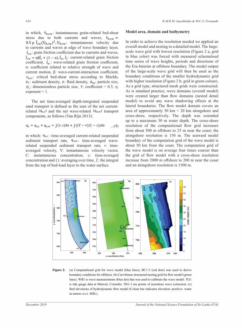
In order to achieve the resolution needed we applied an overall model and nesting to a detailed model. The large-scale wave grid with lowest resolution (Figure 2 a, grid in blue color) was forced with measured schematised time series of wave heights, periods and directions of the Era-Interim at offshore boundary. The model output of the large-scale wave grid will then be used as the boundary conditions of the smaller hydrodynamic grid with higher resolution (Figure 2 b, grid in green colour). As a grid type, structured mesh grids were constructed. As is standard practice, wave domains (overall model) were created larger than flow domains (nested detail model) to avoid any wave shadowing effects at the lateral boundaries. The flow model domain covers an area of approximately 50 km × 20 km alongshore and cross-shore, respectively. The depth was extended up to a maximum 30 m water depth. The cross-shore resolution of the computational flow grid increases from about 500 m offshore to 25 m near the coast; the alongshore resolution is 150 m. The seaward model boundary of the computation grid of the wave model is about 50 km from the coast. The computation grid of the wave model is on average four times coarser than the grid of flow model with a cross-shore resolution increase from 2000 m offshore to 200 m near the coast and an alongshore resolution is 1500 m.
grid of the wave model is about 50 km from the coast. The computation grid of the wave model is on
average four times coarser than the grid of flow model with a cross-shore resolution increases from
2000 m offshore to 200 m near the coast and an alongshore resolution is 1500 m.
Bathymetry data is divided in to offshore and near shore where near-shore data is divided into two
parts: bathymetric and topographic data. For offshore bathymetry, GEBCO, 30 arc second grid
resolution data is used. GEBCO was largely generated by combining quality-controlled ship depth
soundings with interpolation between sounding points guided by satellite-derived gravity data. Near
shore bathymetric data is generated by integrating existing bathymetric data from various sources
such as sounding data from the hydrographic department of National Aquatic Resources Research
and Development Agency (NARA), CCD and large scale nautical charts.
Fig. 2. (a) Computational grid for wave model (blue lines), BC1-3 (red dots) was used to derive boundary conditions for offshore. (b) Curvilinear structured nesting gird for flow model (green lines), WB1 is wave measurements (blue dot) that was used to calibrate the wave model. TG1 is tide gauge data at Mutuwal, Colombo. NS1-3 are points of nearshore wave extraction (c) Bed elevations of hydrodynamic flow model (Colour bar indicates elevation: positive- water in meters w.r.t. MSL).
2.4. Wave climate schematization
ERA-Interim of the European Centre for Medium-Range Weather Forecasts (ECMWF) were used for
the wave boundary of the model. Era interim gives 6 hourly intervals of data over 0.75° x 0.75° grid
resolution. ERA-Interim records between 1979 and 2016 were chosen from three off-shore locations
Commented [m14]: Add details, how reliable the data is, when downloaded etc
Commented [m15]: Introduce first
Commented [m16]: Add the dimensions, X and Y extents, grid sizes, the text is not readable, need to improve
Commented [m17]: Introduce, need some details
Figure 2: (a) Computational grid for wave model (blue lines), BC1-3 (red dots) was used to derive boundary conditions for offshore. (b) Curvilinear structured nesting grid for flow model (green lines). WB1 is wave measurements (blue dot) that was used to calibrate the wave model. TG1 is tide gauge data at Mutwal, Colombo. NS1-3 are points of nearshore wave extraction. (c) Bed elevations of hydrodynamic flow model (Colour bar indicates elevation: positive- water in meters w.r.t. MSL).
Sediment transport - West coast of Sri Lanka 425
Journal of the National Science Foundation of Sri Lanka 47(4) December 2019
Bathymetry data was divided into offshore and near-shore where near-shore data was divided into two parts: bathymetric and topographic data. For offshore bathymetry, GEBCO, 30 arc second grid resolution data was used. GEBCO was largely generated by combining quality-controlled ship depth soundings with interpolation between sounding points guided by satellite-derived gravity data. Nearshore bathymetric data was generated by integrating existing bathymetric data from various sources such as sounding data from the Hydrographic Department of the National Aquatic Resources Research and Development Agency (NARA), CCD and large scale nautical charts.
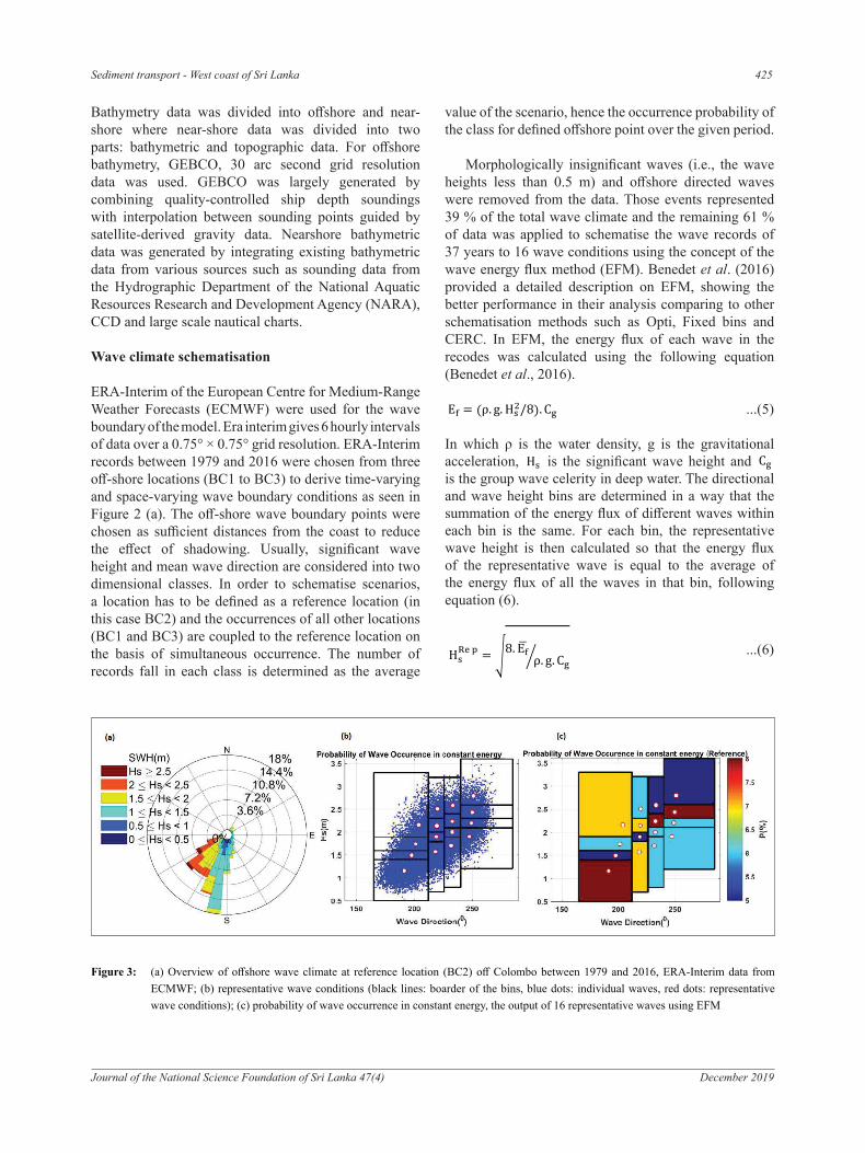
Wave climate schematisation
ERA-Interim of the European Centre for Medium-Range Weather Forecasts (ECMWF) were used for the wave boundary of the model. Era interim gives 6 hourly intervals of data over a 0.75° × 0.75° grid resolution. ERA-Interim records between 1979 and 2016 were chosen from three off-shore locations (BC1 to BC3) to derive time-varying and space-varying wave boundary conditions as seen in Figure 2 (a). The off-shore wave boundary points were chosen as sufficient distances from the coast to reduce the effect of shadowing. Usually, significant wave height and mean wave direction are considered into two dimensional classes. In order to schematise scenarios, a location has to be defined as a reference location (in this case BC2) and the occurrences of all other locations (BC1 and BC3) are coupled to the reference location on the basis of simultaneous occurrence. The number of records fall in each class is determined as the average
value of the scenario, hence the occurrence probability of the class for defined offshore point over the given period.
Morphologically insignificant waves (i.e., the wave heights less than 0.5 m) and offshore directed waves were removed from the data. Those events represented 39 % of the total wave climate and the remaining 61 % of data was applied to schematise the wave records of 37 years to 16 wave conditions using the concept of the wave energy flux method (EFM). Benedet et al. (2016) provided a detailed description on EFM, showing the better performance in their analysis comparing to other schematisation methods such as Opti, Fixed bins and CERC. In EFM, the energy flux of each wave in the recodes was calculated using the following equation (Benedet et al., 2016).
(BC1 to BC3) to derive time-varying and space-varying wave boundary conditions as seen in the
figure 2 (a). The off-shore wave boundary points were chosen as sufficient distances from the coast
to reduce the effect of shadowing. Usually significant wave height and mean wave direction are
considered into two dimensional classes. In order to schematize scenarios, a location has to be defined
as a reference location (in this case BC2) and the occurrences of all other locations (BC1 and BC3)
are coupled to the reference location on the basis of simultaneous occurrence. The number of records
fall in each class is determined the average value of the scenario hence the occurrence probability of
the class for defined offshore point over the given period.
Morphologically insignificant waves (i.e, the wave heights less than 0.5 m) and offshore directed
waves were removed from the data. Those events represented 39% of the total wave climate and the
remaining 61% of data was applied to schematize the wave records of 37 years to 16 wave conditions
using the concept of the wave energy flux method (EFM). In Benedet et al. (2016) a details description
is given on EFM, showing the better performance in their analysis comparing to other schematization
methods such as Opti, Fixed bins and CERC. In EFM, the energy flux (E�) of each wave in the recodes
is calculated using the following eq. (6) (Benedet, Dobrochinski, Walstra, Klein, & Ranasinghe,
2016).
E� = (ρ. g. H��/8). C� (5)
In which ρ is the water density, g is the gravitational acceleration, H� is the significant wave height
and C� is the group wave celerity in deep water. The directional and wave height bins are determined
in a way that the summation of the energy flux of different waves within each bin is the same. For
each bin, the representative wave height is then calculated so that the energy flux of the representative
wave is equal to average of the energy flux of all the waves in that bin, following eq. (6).
H��� � = �8. E��
ρ. g. C�� (6)
In EFM, for example, if the total wave climate is divided into 4 directions and 4 heights (16 bins)
...(5)
In which ρ is the water density, g is the gravitational acceleration,
(BC1 to BC3) to derive time-varying and space-varying wave boundary conditions as seen in the
figure 2 (a). The off-shore wave boundary points were chosen as sufficient distances from the coast
to reduce the effect of shadowing. Usually significant wave height and mean wave direction are
considered into two dimensional classes. In order to schematize scenarios, a location has to be defined
as a reference location (in this case BC2) and the occurrences of all other locations (BC1 and BC3)
are coupled to the reference location on the basis of simultaneous occurrence. The number of records
fall in each class is determined the average value of the scenario hence the occurrence probability of
the class for defined offshore point over the given period.
Morphologically insignificant waves (i.e, the wave heights less than 0.5 m) and offshore directed
waves were removed from the data. Those events represented 39% of the total wave climate and the
remaining 61% of data was applied to schematize the wave records of 37 years to 16 wave conditions
using the concept of the wave energy flux method (EFM). In Benedet et al. (2016) a details description
is given on EFM, showing the better performance in their analysis comparing to other schematization
methods such as Opti, Fixed bins and CERC. In EFM, the energy flux (E�) of each wave in the recodes
is calculated using the following eq. (6) (Benedet, Dobrochinski, Walstra, Klein, & Ranasinghe,
2016).
E� = (ρ. g. H��/8). C� (5)
In which ρ is the water density, g is the gravitational acceleration, H� is the significant wave height
and C� is the group wave celerity in deep water. The directional and wave height bins are determined
in a way that the summation of the energy flux of different waves within each bin is the same. For
each bin, the representative wave height is then calculated so that the energy flux of the representative
wave is equal to average of the energy flux of all the waves in that bin, following eq. (6).
H��� � = �8. E��
ρ. g. C�� (6)
In EFM, for example, if the total wave climate is divided into 4 directions and 4 heights (16 bins)
is the significant wave height and
(BC1 to BC3) to derive time-varying and space-varying wave boundary conditions as seen in the
figure 2 (a). The off-shore wave boundary points were chosen as sufficient distances from the coast
to reduce the effect of shadowing. Usually significant wave height and mean wave direction are
considered into two dimensional classes. In order to schematize scenarios, a location has to be defined
as a reference location (in this case BC2) and the occurrences of all other locations (BC1 and BC3)
are coupled to the reference location on the basis of simultaneous occurrence. The number of records
fall in each class is determined the average value of the scenario hence the occurrence probability of
the class for defined offshore point over the given period.
Morphologically insignificant waves (i.e, the wave heights less than 0.5 m) and offshore directed
waves were removed from the data. Those events represented 39% of the total wave climate and the
remaining 61% of data was applied to schematize the wave records of 37 years to 16 wave conditions
using the concept of the wave energy flux method (EFM). In Benedet et al. (2016) a details description
is given on EFM, showing the better performance in their analysis comparing to other schematization
methods such as Opti, Fixed bins and CERC. In EFM, the energy flux (E�) of each wave in the recodes
is calculated using the following eq. (6) (Benedet, Dobrochinski, Walstra, Klein, & Ranasinghe,
2016).
E� = (ρ. g. H��/8). C� (5)
In which ρ is the water density, g is the gravitational acceleration, H� is the significant wave height
and C� is the group wave celerity in deep water. The directional and wave height bins are determined
in a way that the summation of the energy flux of different waves within each bin is the same. For
each bin, the representative wave height is then calculated so that the energy flux of the representative
wave is equal to average of the energy flux of all the waves in that bin, following eq. (6).
H��� � = �8. E��
ρ. g. C�� (6)
In EFM, for example, if the total wave climate is divided into 4 directions and 4 heights (16 bins)
is the group wave celerity in deep water. The directional and wave height bins are determined in a way that the summation of the energy flux of different waves within each bin is the same. For each bin, the representative wave height is then calculated so that the energy flux of the representative wave is equal to the average of the energy flux of all the waves in that bin, following equation (6).
(BC1 to BC3) to derive time-varying and space-varying wave boundary conditions as seen in the
figure 2 (a). The off-shore wave boundary points were chosen as sufficient distances from the coast
to reduce the effect of shadowing. Usually significant wave height and mean wave direction are
considered into two dimensional classes. In order to schematize scenarios, a location has to be defined
as a reference location (in this case BC2) and the occurrences of all other locations (BC1 and BC3)
are coupled to the reference location on the basis of simultaneous occurrence. The number of records
fall in each class is determined the average value of the scenario hence the occurrence probability of
the class for defined offshore point over the given period.
Morphologically insignificant waves (i.e, the wave heights less than 0.5 m) and offshore directed
waves were removed from the data. Those events represented 39% of the total wave climate and the
remaining 61% of data was applied to schematize the wave records of 37 years to 16 wave conditions
using the concept of the wave energy flux method (EFM). In Benedet et al. (2016) a details description
is given on EFM, showing the better performance in their analysis comparing to other schematization
methods such as Opti, Fixed bins and CERC. In EFM, the energy flux (E�) of each wave in the recodes
is calculated using the following eq. (6) (Benedet, Dobrochinski, Walstra, Klein, & Ranasinghe,
2016).
E� = (ρ. g. H��/8). C� (5)
In which ρ is the water density, g is the gravitational acceleration, H� is the significant wave height
and C� is the group wave celerity in deep water. The directional and wave height bins are determined
in a way that the summation of the energy flux of different waves within each bin is the same. For
each bin, the representative wave height is then calculated so that the energy flux of the representative
wave is equal to average of the energy flux of all the waves in that bin, following eq. (6).
H��� � = �8. E��
ρ. g. C�� (6)
In EFM, for example, if the total wave climate is divided into 4 directions and 4 heights (16 bins)
...(6)
each bin represents 1/16 of the total energy (E/16). Figure 3 shows the procedure of the wave
schematization, and the results of 16 schematized wave conditions that were computed are presented
in table 1.
Fig. 3. (a) Overview of offshore wave climate at reference location (BC2) off Colombo between 1979 and 2016, ERA-Interim data from ECMWF (b) Representative wave conditions (black lines: boarder of the bins, blue dots: individual waves red dots: representative wave conditions) (c) Probability of wave occurrence in constant energy, the output of 16 representative waves using EFM.
2.5. The Morfac Approach
The morphological acceleration factor (MORFAC) concept is applied in this study. The MORFAC
approach multiplies the bed levels computed after each hydrodynamic time step by a factor
(MORFAC) to enable much faster computation (Ranasinghe, 2011; Roelvink 2006). The significantly
up scaled new bathymetry is then used in the next hydrodynamic step. During a morphological
simulation, each of the selected wave conditions is simulated for the duration of one morphological
tide (i.e 12 hours 25 minutes = 745 mins) in order to account for the random phasing between waves
and tides that occurs in nature. For each wave condition the morphological acceleration factor applied
will depend on the percentage occurrence (days per year) of that particular wave condition. The
morphological acceleration factors applied to each wave condition are indicated in table 1.
Table 2. The resulting reduced wave climate. In the last column, the morphological acceleration factors for the different wave conditions are shown.
Condition Hs (m)
Tp (s)
Direction (0)
Occurrence (days)
Morfac
1 1.16 9.76 191.46 72.61 143.62 2 1.50 9.82 197.68 26.06 51.54 3 1.74 9.95 201.41 26.11 51.65 4 2.16 10.52 203.90 20.21 39.98
Figure 3: (a) Overview of offshore wave climate at reference location (BC2) off Colombo between 1979 and 2016, ERA-Interim data from ECMWF; (b) representative wave conditions (black lines: boarder of the bins, blue dots: individual waves, red dots: representative wave conditions); (c) probability of wave occurrence in constant energy, the output of 16 representative waves using EFM
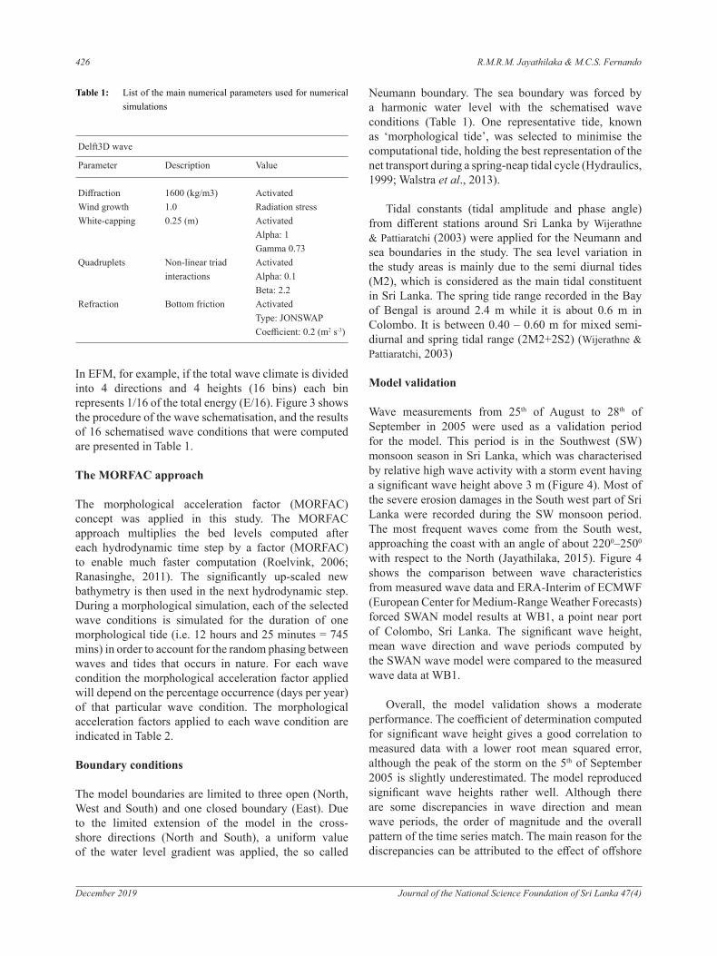
426 R.M.R.M. Jayathilaka & M.C.S. Fernando
December 2019 Journal of the National Science Foundation of Sri Lanka 47(4)
Neumann boundary. The sea boundary was forced by a harmonic water level with the schematised wave conditions (Table 1). One representative tide, known as ‘morphological tide’, was selected to minimise the computational tide, holding the best representation of the net transport during a spring-neap tidal cycle (Hydraulics, 1999; Walstra et al., 2013).
Tidal constants (tidal amplitude and phase angle) from different stations around Sri Lanka by Wijerathne & Pattiaratchi (2003) were applied for the Neumann and sea boundaries in the study. The sea level variation in the study areas is mainly due to the semi diurnal tides (M2), which is considered as the main tidal constituent in Sri Lanka. The spring tide range recorded in the Bay of Bengal is around 2.4 m while it is about 0.6 m in Colombo. It is between 0.40 – 0.60 m for mixed semi-diurnal and spring tidal range (2M2+2S2) (Wijerathne & Pattiaratchi, 2003)
Model validation
Wave measurements from 25th of August to 28th of September in 2005 were used as a validation period for the model. This period is in the Southwest (SW) monsoon season in Sri Lanka, which was characterised by relative high wave activity with a storm event having a significant wave height above 3 m (Figure 4). Most of the severe erosion damages in the South west part of Sri Lanka were recorded during the SW monsoon period. The most frequent waves come from the South west, approaching the coast with an angle of about 2200–2500 with respect to the North (Jayathilaka, 2015). Figure 4 shows the comparison between wave characteristics from measured wave data and ERA-Interim of ECMWF (European Center for Medium-Range Weather Forecasts) forced SWAN model results at WB1, a point near port of Colombo, Sri Lanka. The significant wave height, mean wave direction and wave periods computed by the SWAN wave model were compared to the measured wave data at WB1.
Overall, the model validation shows a moderate performance. The coefficient of determination computed for significant wave height gives a good correlation to measured data with a lower root mean squared error, although the peak of the storm on the 5th of September 2005 is slightly underestimated. The model reproduced significant wave heights rather well. Although there are some discrepancies in wave direction and mean wave periods, the order of magnitude and the overall pattern of the time series match. The main reason for the discrepancies can be attributed to the effect of offshore
Delft3D wave
Parameter Description Value
Diffraction 1600 (kg/m3) Activated Wind growth 1.0 Radiation stressWhite-capping 0.25 (m) Activated Alpha: 1 Gamma 0.73 Quadruplets Non-linear triad Activated interactions Alpha: 0.1 Beta: 2.2 Refraction Bottom friction Activated Type: JONSWAP Coefficient: 0.2 (m2 s-3)
Table 1: List of the main numerical parameters used for numerical simulations
In EFM, for example, if the total wave climate is divided into 4 directions and 4 heights (16 bins) each bin represents 1/16 of the total energy (E/16). Figure 3 shows the procedure of the wave schematisation, and the results of 16 schematised wave conditions that were computed are presented in Table 1.
The MORFAC approach
The morphological acceleration factor (MORFAC) concept was applied in this study. The MORFAC approach multiplies the bed levels computed after each hydrodynamic time step by a factor (MORFAC) to enable much faster computation (Roelvink, 2006; Ranasinghe, 2011). The significantly up-scaled new bathymetry is then used in the next hydrodynamic step. During a morphological simulation, each of the selected wave conditions is simulated for the duration of one morphological tide (i.e. 12 hours and 25 minutes = 745 mins) in order to account for the random phasing between waves and tides that occurs in nature. For each wave condition the morphological acceleration factor applied will depend on the percentage occurrence (days per year) of that particular wave condition. The morphological acceleration factors applied to each wave condition are indicated in Table 2.
Boundary conditions
The model boundaries are limited to three open (North, West and South) and one closed boundary (East). Due to the limited extension of the model in the cross-shore directions (North and South), a uniform value of the water level gradient was applied, the so called
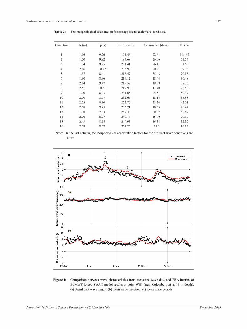
Sediment transport - West coast of Sri Lanka 427
Journal of the National Science Foundation of Sri Lanka 47(4) December 2019
Table 2: The morphological acceleration factors applied to each wave condition.
Condition Hs (m) Tp (s) Direction (0) Occurrence (days) Morfac
1 1.16 9.76 191.46 72.61 143.62 2 1.50 9.82 197.68 26.06 51.54 3 1.74 9.95 201.41 26.11 51.65 4 2.16 10.52 203.90 20.21 39.98 5 1.57 8.41 218.47 35.48 70.18 6 1.90 8.96 219.12 18.44 36.48 7 2.14 9.47 219.52 19.39 38.36 8 2.51 10.21 219.96 11.40 22.56 9 1.70 8.03 231.65 25.51 50.47 10 2.00 8.57 232.65 18.14 35.88 11 2.23 8.96 232.76 21.24 42.01 12 2.58 9.45 233.21 10.35 20.47 13 1.90 7.84 247.43 20.57 40.69 14 2.20 8.27 249.13 15.00 29.67 15 2.43 8.54 249.95 16.34 32.32 16 2.79 8.77 251.26 8.16 16.15
Note: In the last column, the morphological acceleration factors for the different wave conditions are shown.
Fig. 4 Comparison between wave characteristics from measured wave data and ERA-Interim of ECMWF forced SWAN model results at point WB1 (near Colombo port at 19 m depth). (a) Significant wave height; (b) mean wave direction; (c) mean wave periods.
3. Results and Discussion
3.1. Wind/Wave analysis
The northern Indian Ocean is characterized by bi-annually reversing monsoon winds resulting from
the seasonal differential heating and cooling of the continental land mass and the ocean. The SW
monsoon generally operates between June and October, and the NE monsoon operates from
December through April (Tomczak & Godfrey, 2003). The transition periods are termed the first inter-
monsoon (May) and the second inter-monsoon (November). We studied 37 years (from 1979 to 2016)
of ERA-Interim data to schematize the wind/wave climate for boundary conditions.
According to the wind climate in the study area, wind is coming from NE direction from November
to March with the angle 400-600 while it changes to SW direction with the angle 2200-2400 from May
to September. During SW monsoon, the wind speed varies between 7-11 m/s while it varies between
1-5 m/s during NE monsoon. The total number of wind-wave events studied here is 54053 during
Commented [m20]: Not under Reference Inserted
Figure 4: Comparison between wave characteristics from measured wave data and ERA-Interim of ECMWF forced SWAN model results at point WB1 (near Colombo port at 19 m depth). (a) Significant wave height; (b) mean wave direction; (c) mean wave periods.
Mea
n w
ave
perio
ds (s
)M
ean
wav
e di
rect
ion
(deg
)
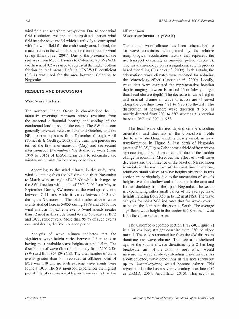
428 R.M.R.M. Jayathilaka & M.C.S. Fernando
December 2019 Journal of the National Science Foundation of Sri Lanka 47(4)
wind field and nearshore bathymetry. Due to poor wind field resolution, we applied interpolated coarser wind field into the wave model which is unlikely to correspond with the wind field for the entire study area. Indeed, the inaccuracies in the variable wind field can affect the wind set up (Elias et al., 2001). Due to the presence of the reef area from Mount Lavinia to Colombo, a JONSWAP coefficient of 0.2 was used to represent the higher bottom friction in reef areas. Default JONSWAP coefficient (0.064) was used fer the area between Colombo to Negombo.
RESULTS AND DISCUSSION
Wind/wave analysis
The northern Indian Ocean is characterised by bi-annually reversing monsoon winds resulting from the seasonal differential heating and cooling of the continental land mass and the ocean. The SW monsoon generally operates between June and October, and the NE monsoon operates from December through April (Tomczak & Godfrey, 2003). The transition periods are termed the first inter-monsoon (May) and the second inter-monsoon (November). We studied 37 years (from 1979 to 2016) of ERA-Interim data to schematise the wind/wave climate for boundary conditions.
According to the wind climate in the study area, wind is coming from the NE direction from November to March with an angle of 400–600 while it changes to the SW direction with angle of 2200–2400 from May to September. During SW monsoon, the wind speed varies between 7–11 m/s while it varies between 1×5 m/s during the NE monsoon. The total number of wind-wave events studied here is 54053 during 1979 and 2015. The wind analysis for extreme events (wind speeds greater than 12 m/s) in this study found 43 and 65 events at BC2 and BC3, respectively. More than 95 % of such events occurred during the SW monsoon period.
Analysis of wave climate indicates that the significant wave height varies between 0.5 m to 3 m having most probable wave heights around 1.5 m. The distribution of wave direction is mostly from 2100–2500 (SW) and from 300–800 (NE). The total number of wave events greater than 3 m recorded at offshore point of BC2 was 149 and no such extreme wave events were found at BC3. The SW monsoon experiences the highest probability of occurrence of higher wave events than the
NE monsoon.Wave transformation (SWAN)
The annual wave climate has been schematised to 16 wave conditions accompanied by the relative morphological acceleration factors that represent the net transport occurring in one-year period (Table 2). The wave chronology plays a significant role in process based modelling (Lesser et al., 2009). In this study, the schematised wave climates were repeated for reducing the ‘chronology effect’ (Lesser et al., 2009). Locally, wave data were extracted for representative location depths ranging between 10 m and 15 m (always larger than local closure depth). The decrease in wave heights and gradual change in wave direction are observed along the coastline from NS1 to NS3 (northward). The distribution of near-shore wave direction at NS1 is mostly directed from 2300 to 2500 whereas it is varying between 2600 and 2900 at NS3.
The local wave climates depend on the shoreline orientation and steepness of the cross-shore profile due to wave shielding, which is clearly visible in wave transformation in Figure 5. Just north of Negombo (section P30-35, Figure 7) the coast is shielded from waves approaching the southern directions due to the sudden change in coastline. Moreover, the effect of swell wave decreases and the influence of the onset of NE monsoon is visible in the northward of the coast line. Therefore, relatively small values of wave heights observed in this section are particularly due to the attenuation of wave’s heights over the shallow and mild slope in the area and further shielding from the tip of Negombo. The sector is experiencing rather small values of the average wave heights, ranging from 0.50 m to 1.2 m at NS3. The wave analysis for point NS3 indicates that for waves over 1 m height the dominant direction is South. The average significant wave height in the section is 0.8 m, the lowest from the entire studied zone.
The Colombo-Negombo section (P12-30, Figure 7) is a 30 km long straight coastline with 2500 to shore normal. The waves approaching from the SW directions dominate the wave climate. This sector is sheltered against the southern wave directions by a 2 km long breakwater arm of the Colombo port, which would increase the wave shadow, extending it northwards. As a consequence, wave conditions in this area (probably up to Uswatakeiyawa) would become calmer. This region is identified as a severely eroding coastline (CC & CRMD, 2004; Jayathilaka, 2015). This sector is
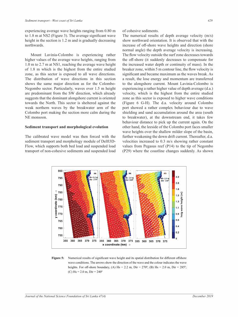
Sediment transport - West coast of Sri Lanka 429
Journal of the National Science Foundation of Sri Lanka 47(4) December 2019
experiencing average wave heights ranging from 0.80 m to 1.8 m at NS2 (Figure 3). The average significant wave height in the section is 1.2 m and is gradually decreasing northwards.
Mount Lavinia-Colombo is experiencing rather higher values of the average wave heights, ranging from 1.0 m to 2.7 m at NS1, reaching the average wave height of 1.8 m which is the highest from the entire studied zone, as this sector is exposed to all wave directions. The distribution of wave directions in this section shows the same major direction as for the Colombo-Negombo sector. Particularly, waves over 1.5 m height are predominant from the SW direction, which already suggests that the dominant alongshore current is oriented towards the North. This sector is sheltered against the weak northern waves by the breakwater arm of the Colombo port making the section more calm during the NE monsoon.
Sediment transport and morphological evolution
The calibrated wave model was then forced with the sediment transport and morphology module of Delft3D-Flow, which supports both bed load and suspended load transport of non-cohesive sediments and suspended load
of cohesive sediments. The numerical results of depth average velocity (m/s) show northward orientation. It is observed that with the increase of off-shore wave heights and direction (shore normal angle) the depth average velocity is increasing. The flow velocity outside the surf zone decreases towards the off-shore (it suddenly decreases to compensate for the increased water depth or continuity of mass). In the breaker zone, within 5 m contour line, the flow velocity is significant and became maximum as the waves break. As a result, the lose energy and momentum are transferred to the alongshore current. Mount Lavinia-Colombo is experiencing a rather higher value of depth average (d.a.) velocity, which is the highest from the entire studied zone as this sector is exposed to higher wave conditions (Figure 6 G-H). The d.a. velocity around Colombo port showed a rather complex behaviour due to wave shielding and sand accumulation around the area (south to breakwater), at the downstream end, it takes few behaviour distance to pick up the current again. On the other hand, the leeside of the Colombo port faces smaller wave heights over the shallow milder slope of the basin, further weakening the down drift current. Thereafter, d.a. velocities increased to 0.3 m/s showing rather constant values from Pegasus reef (P14) to the tip of Negombo (P29) where the coastline changes suddenly. As shown
Fig. 5. Numerical results of significant wave height and its spatial distribution for different offshore wave conditions. The arrows show the direction of the wave and the color indicate the wave heights. For off-shore boundary, (A) Hs=2.2 m, Dir=2700 (B) Hs=2.0 m, Dir=2850 (C) Hs=2.0 m, Dir=2400
The local wave climates depend on the shoreline orientation and steepness of the cross-shore profile
due to wave shielding which is clearly visible in wave transformation in figure 5. Just north of
Negombo (section P30-35, Fig. 7) the coast is shielded from waves approaching the southern
directions due to the sudden change in coastline. Moreover, the effect of swell wave decreases and
the influence of onset of NE monsoon are visible in the northward of the coast line. Therefore,
relatively small values of wave heights observed in this section are particularly due to the attenuation
of wave’s heights over the shallow and mild slope in the area and further shielding from the tip of
Negombo. The sector is experiencing rather small values of the average wave heights, ranging from
0.50 m to 1.2 m at NS3. The wave analysis for point NS3 indicates that for waves over 1 m height
the dominant direction is from south. The average significant wave height in the section is 0.8 m, the
lowest from the entire studied zone.
The Colombo-Negombo section (P12-30, Fig. 7) is a straight coastline having 30 km long and 2500
degree to shore normal. The waves approaching from the SW directions dominate the wave climate.
This sector is sheltered against the southern wave directions by 2 km long breakwater arm of Colombo
port which would increase the wave shadow, extending it northwards. As a consequence, wave
Commented [m21]: ?
Figure 5: Numerical results of significant wave height and its spatial distribution for different offshore wave conditions. The arrows show the direction of the wave and the colour indicates the wave heights. For off-shore boundary, (A) Hs = 2.2 m, Dir = 2700; (B) Hs = 2.0 m, Dir = 2850; (C) Hs = 2.0 m, Dir = 2400
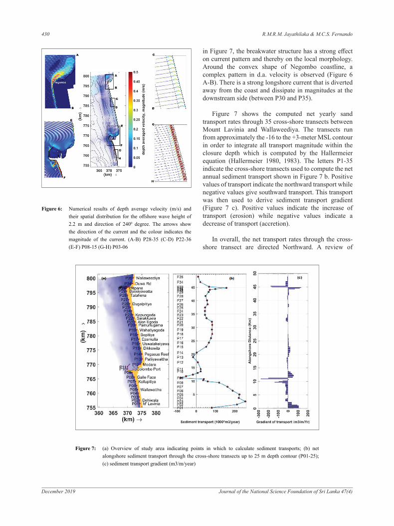
430 R.M.R.M. Jayathilaka & M.C.S. Fernando
December 2019 Journal of the National Science Foundation of Sri Lanka 47(4)
Fig. 7. (a) Overview of study area indicating points in which to calculate sediment transports. (b) Net alongshore sediment transport through the cross-shore transects up to 25 m depth contour (P01-25). (c) Sediment transport gradient (m3/m/year)
In overall, the net transports rates through the cross-shore transect are directed to the Northward. A
review of several publications and technical reports about sediment transport along SW coast of Sri
Lanka indicate northward transport (Ansaf, 2012; CC&CRMD, 2004; Jayathilaka, 2015; Laknath &
Sasaki, 2011). The net sediment transport capacity computed between M’ Lavinia (P1) and Colombo
(P8) shows the maximum value of the transport capacity for the whole studied area is reached, 255
000 m3/year (P3) and then gradually decreased to 90 000 m3/year near Galle Face (P8). In this sector
the wave climate and, subsequently, the gross alongshore transport reach the highest values indicating
a relative dynamic environment. The two important factors contributing to this are the full exposure
of the southern side of the island to swell and wind waves during the SW monsoon and the rather
steep slope of the beach comparing to Colombo (P10)-Negombo (P35) coastline (Jayathilaka, 2015).
The transport rates in M’ Lavinia-Colombo is in general less than the transport rates shown by
previous studies (Ansaf, 2012; Jayathilaka, 2015). According to CCD-GTZ Coast Conservation
Project in 1992, the estimated along shore transport rate in this section varies between 460,000
m3/year to 1,180,000 m3/year. The separate studies of MIKE21 and UNIBEST ST showed same
Commented [m32]: Not the right way to cite
Figure 7: (a) Overview of study area indicating points in which to calculate sediment transports; (b) net alongshore sediment transport through the cross-shore transects up to 25 m depth contour (P01-25); (c) sediment transport gradient (m3/m/year)
Fig. 6. Numerical results of depth average velocity (m/s) and their spatial distribution for the offshore wave height of 2.2 m and direction of 2400 degree. The arrows show the direction of the current and the colour indicate the magnitude of the current. (A-B) P28-35 (C-D) P22-36 (E-F) P08-15 (G-H) P03-06
The numerical results of depth average velocity (m/s) shows northward oriented. It is observed that
with the increase of off-shore wave heights and direction (shore normal angle) the depth average
velocity is increasing. The flow velocity outside surf zone decreases towards the off-shore (it
suddenly decreases to compensate for the increased water depth or continuity of mass). In the breaker
zone, within 5 m contour line, the flow velocity is significant and became maximum as the wave
break. As a result, the lose energy and momentum is transferred to the alongshore current. Mount
Lavinia-Colombo is experiencing rather higher value of depth average (d.a) velocity which is the
highest from the entire studied zone as this sector is exposed to higher wave conditions (Fig. 6 G-H).
The d.a velocity around Colombo port showed rather complex behaviour due to wave shielding and
Commented [m23]: Cannot see the direction of the arrows,
Commented [m24]: ?
Commented [m25]: ?
Commented [m26]: ?
Figure 6: Numerical results of depth average velocity (m/s) and their spatial distribution for the offshore wave height of 2.2 m and direction of 2400 degree. The arrows show the direction of the current and the colour indicates the magnitude of the current. (A-B) P28-35 (C-D) P22-36 (E-F) P08-15 (G-H) P03-06
in Figure 7, the breakwater structure has a strong effect on current pattern and thereby on the local morphology. Around the convex shape of Negombo coastline, a complex pattern in d.a. velocity is observed (Figure 6 A-B). There is a strong longshore current that is diverted away from the coast and dissipate in magnitudes at the downstream side (between P30 and P35).
Figure 7 shows the computed net yearly sand transport rates through 35 cross-shore transects between Mount Lavinia and Wallaweediya. The transects run from approximately the -16 to the +3-meter MSL contour in order to integrate all transport magnitude within the closure depth which is computed by the Hallermeier equation (Hallermeier 1980, 1983). The letters P1-35 indicate the cross-shore transects used to compute the net annual sediment transport shown in Figure 7 b. Positive values of transport indicate the northward transport while negative values give southward transport. This transport was then used to derive sediment transport gradient (Figure 7 c). Positive values indicate the increase of transport (erosion) while negative values indicate a decrease of transport (accretion).
In overall, the net transport rates through the cross-shore transect are directed Northward. A review of
Sediment transport - West coast of Sri Lanka 431
Journal of the National Science Foundation of Sri Lanka 47(4) December 2019
several publications and technical reports about sediment transport along the SW coast of Sri Lanka indicates northward transport (CC&CRMD, 2004; Laknath & Sasaki, 2011; Ansaf, 2012; Jayathilaka, 2015). The net sediment transport capacity computed between Mount Lavinia (P1) and Colombo (P8) shows the maximum value of the transport capacity for the whole studied area reached as 255,000 m3/year (P3) and then gradually decreased to 90,000 m3/year near Galle Face (P8). In this sector the wave climate and subsequently, the gross alongshore transport reach the highest values indicating a relative dynamic environment. The two important factors contributing to this are the full exposure of the southern side of the island to swell and wind waves during the SW monsoon and the rather steep slope of the beach compared to Colombo (P10)-Negombo (P35) coastline (Jayathilaka, 2015).
The transport rates in Mount Lavinia - Colombo are in general less than the transport rates shown by previous studies (Ansaf, 2012; Jayathilaka, 2015). According to CCD-GTZ Coast Conservation Project in 1992, the estimated alongshore transport rate in this section varies between 460,000 m3/year to 1,180,000 m3/year. The separate studies of MIKE21 and UNIBEST ST showed same magnitudes of the northward net transport rate along the same coastline (Anfas, 2012; Jayathilaka, 2015). The main reason for these higher values of transport rates was not including the presence of reefs and the beach rock laying parallel to the Mount Lavinia - Colombo coastline. The greater width of non-mobile topology, which deceases the sediment transport due to roughness plays a significant role on calibrating behaviour sediment transport to actual sediment transport. In the present study, we have introduced spatial varying roughness parameter (JONSWAP coefficient) to estimate coastal transport rates for the various coastal segments between Mount Lavinia-Colombo and Colombo-Negombo as discussed in model validation.
The southern breakwater arm of the Colombo South Port (2 km long) shows the strong effect on transport gradient (Figure 7 c). The shoreline upstream of the structure accretes rapidly and the coast downward shows rapid erosion. The seaward end of the breakwater will be in about 18 m depth of water, which is far deeper than the depth of closure where most of the sediment transport occurs. Therefore, a significant proportion of sand transport is captured by the breakwater arm in which it accumulates against the breakwater. Over time the area of accumulation will extend both seawards and southwards along the coast where the ongoing Port City Development Project is located. The behaviour of the
down drift side of the breakwater depends on the process of building of the longshore current. The slow building of the longshore current leads the long area of extends for erosion. Figure 7c shows positive values in sediment gradients between Modara (P10) to Uswatakeiyawa (P16). This region is identified as a severely eroding coastline (CC & CRMD, 2004; Bureau, 2005; Jayathilaka, 2015; Wijayawardane et al., 2013). In the Master Plan for Coast Erosion Management Summary, the erosion rate was identified as 2.5 m/year for 70 % of the coastline from Palliyawatte (P13) to Uswetikeiyawa (P16). Decrease in sand supply from the Kaleni river located between P12 and P13 is said to accelerate the down drift erosion north of the river mouth (CC & CRMD, 2004). A nodal point, the transport direction changed and building is observed behind Pegasus Reef. Thereafter, 55 000 m3/year rate of transport shown in Dikkowita (P15) and to reached 90 000 m3/year near Pamunugama (P20) with a milder gradient along the straight coastline. Then the coastline bends slightly extending to Bassiyawattha (P29) and afterwards the coastline exhibits a convex form. In the area between Bassiyawattha (P29) and Pitipana (P33) the transport is increasing with a steep gradient, suggesting intense erosion (Figure 7c). The convex shape of the coastline shields the down drift side of Pitipana from wave action, preventing much longshore drift where waves are not strong enough to move the sediment along the coast.
CONCLUSION
The main contribution of this work is the quantitative determination of a nearshore wave climate, the alongshore sediment transport along 55 km long coastal belt between Mount Lavinia and Negombo. Delft3D-FLOW, a process-based model, modeled together with input reduction and morphological acceleration techniques has been used to estimate the long shore sediment transport rates and related morphodynamics. The importance of nearshore wave transformation is highlighted in the conclusion. In data poor environment, this is achieved by transforming offshore wave time series (schematised) to nearshore locations (SWAN model). The final reduced set of forcing conditions (16 conditions) is supposed to be sufficient enough to capture the morphological change to its full extent. However, certain low probability, high-energy conditions responsible for alongshore sediment transport can also be included for better model results. The simulated wave climate based on wind records proved to be reliable despite the lack of precise data. The numerical results can very well be related to the accuracy of bathymetry or measured wave buoy data
432 R.M.R.M. Jayathilaka & M.C.S. Fernando
December 2019 Journal of the National Science Foundation of Sri Lanka 47(4)
or both. Default parameter settings and coefficients in Delft3D such as depth induced breaking, non-linear triad interactions and bottom friction applied during simulation, show quite unrealistic results and have to tune accordingly. Increased coverage and accuracy of wave measurements would probably provide the greatest improvements in future studies. Therefore, at least one wave buoy should deploy between Colombo and Negombo where the shoreline orientation changes abruptly.
The wave model is calibrated and reproduces nearshore waves well. Analysis of model results indicated that the Southwest monsoon has greater influences having the highest probability of occurrence of higher wave events on the near-shore wave climate, thus sediment transport in the study area. More than 95 % of the extreme events occurred during the SW monsoon periods. However, the effect of swell wave decreases and the influence of onset of NE monsoon are visible when it goes to the northward of the coastline. Mount Lavinia-Colombo coastline shows the highest wave heights from the entire studied area, thus rather higher value of d.a. velocity than in Colombo-Negombo coastline. Numerical results of the alongshore sediment transport gradients clearly indicate the potential erosion/accretion prone areas, emphasising the importance of detailed coastal morphological studies and quantitative risk assessments at vulnerable coastal areas along the coast of Mount Lavinia-Negombo. The study shows that the Colombo-Negombo coastline is naturally subjected to erosion due to its coastal orientation and wave actions. To compensate the erosion rate, the importance of a steady sand supply from the Kaleni river is highlighted. The reduction of sand supply from the Kaleni river due to extensive sand mining is a contributory factor that accelerates the coastal erosion in that area. In addition, the breakwater of Colombo port has a partial effect on changing the local erosion/accretion rates in the area extending to adjacent coastal areas. Sand nourishment in the down drift area is a nature- friendly method to restore the regional sediment budget in the area. This requires the complete stop of sand mining in rivers and sea-sand dredging within the closure depth.
Acknowledgements
The authors wish to thank all the staff members of Oceanography Division of the National Aquatic Resources Research and Development Agency (NARA) for their valuable assistance during field and laboratory work. This work was conducted under the research
project on Sediment Transport Studies in West Coast of Sri Lanka funded by NARA. The authors would like to thank the anonymous reviewers for their valuable comments that helped improve the quality of this paper significantly.
REFERENCES
Ansaf K.M.M. (2012). Investigations on coastal sediment transport and shoreline behaviour. Msc thesis, Dept. of Civil Engineering, University of Moratuwa, Sri Lanka. Available at http://dl.lib.mrt.ac.lk/handle/123/2049. Accessed 9 March 2018
Benedet L., Dobrochinski J., Walstra D., Klein A. & Ranasinghe R. (2016). A morphological modeling study to compare different methods of wave climate schematization and evaluate strategies to reduce erosion losses from a beach nourishment project. Coastal Engineering 112: 69-86.
DOI: https://doi.org/10.1016/j.coastaleng.2016.02.005. Bureau C.E.C. (2005). Supplementary Environmental
Impact Assessment Report, Proposed Colombo Port City Development Project. Available at http://ejustice.lk/2017/10/21/port-city-suplimentory-eia-report/. Accessed 5 October 2017.
Coast Conservation and Coastal Resource Management Department (CC & CRMD) (2004). Coastal Zone Management Plan (CZMP). Part I Section I Gazzet Extraordinary of the Democratic Socialist Republic of Sri Lanka. Available at http://www.coastal.gov.lk/downloads/pdf/CZMPEnglish.pdf.
Duong T.M., Ranasinghe R., Walstra D. & Roelvink D. (2016). Assessing climate change impacts on the stability of small tidal inlet systems: why and how?. Earth-Science Reviews 154: 369-380.
DOI: https://doi.org/10.1016/j.margeo.2017.09.007Elias E.P.L., Walstra D.J.R., Roelvink J.A., Stive M.J.F. &
Klein M.D. (2001). Hydrodynamic validation of Delft3D with field measurements at Egmond. Coastal Engineering pp. 2714-2727.
DOI: https://doi.org/10.1061/40549(276)212 Fittschen T., Perera J.A.S.C. & Scheffer H.J. (1992). Sediment
Transport Study for the Southwest Coast of Sri Lanka, CCD – GTZ Coast Conservation Project, Coastal Conservation Department of Sri Lanka.
Garcin M., Desprats J.F., Fontaine M., Pedreros R., Attanayake N., Fernando S. & Poisson B. (2008). Integrated approach for coastal hazards and risks in Sri Lanka. Natural Hazards and Earth System Sciences 8: 577-586.
Giardino A., Van der Werf J. & Van Ormondt M. (2010). Simulating Coastal Morphodynamics with Delft3D: case study Egmond aan Zee. PhD-thesis. Delft University of Technology.
DOI: https://doi.org/10.13140/2.1.2596.9925Gunarathna P., Ranasinghe D. & Sugandika T. (2011).
Assessment of nearshore wave climate off the Southern Coast of Sri Lanka. Journal of the Institution of Engineers,
Sediment transport - West coast of Sri Lanka 433
Journal of the National Science Foundation of Sri Lanka 47(4) December 2019
Sri Lanka, 44(2):33-42. DOI: https://doi.org/10.4038/engineer.v44i2.7021 Hallermeier R. J. (1980). A profile zonation for seasonal sand
beaches from wave climate. Coastal Engineering 4: 253-277.
DOI: https://doi.org/10.1016/0378-3839(80)90022-8Hallermeier R.J. (1983). Sand transportation limits in coastal
structure designs. In Coastal Structures’ 83, Washington D.C., March 9-11, 1983, pp. 703-716. Available at https://ascelibrary.org/doi/abs/10.1061
Hydraulics D. (1999). User Manual Delft3D-FLOW. Wl Delft Hydraulics, The Netherlands.
Hydraulics D. (2006). User Manual Delft3D-WAVE, Simulation of short-crested waves with SWAN. Wl Delft Hydraulics, The Netherlands.
Hydraulics W.D. (2006). User Manual Delft3D-FLOW, Simulation of multi-dimensional hydrodynamic flows and transport phenomena, including sediments, Wl Delft Hydraulics, The Netherlands.
Jayathilaka R. (2015). MSc thesis, Large scale sediment budgets in data poor environments via numerical modelling: case study of Sri Lanka’s south-west coast. UNESCO-IHE, Delft, The Netherlands.
Laknath D. & Sasaki J. (2011). Wave Climate Study around Kirinda Fishery Harbour in Sri Lanka using SWAN Model. International Offshore and Polar Engineering Conference, Hawaii, USA, June 19-24.
Lesser G.R., Roelvink J.V., Van Kester J.A.T.M. & Stelling G.S. (2004). Development and validation of a three-dimensional morphological model. Coastal Engineering 51(8-9): 883-915.
DOI: https://doi.org/10.1016/j.coastaleng.2004.07.014Lesser G.R. (2009). An approach to medium-term coastal
morphological modelling. PhD Thesis, UNESCO-IHE, Institute for Water Education, Delft, The Netherlands.
Ranasinghe R., Swinkels C., Luijendijk A., Roelvink D., Bosboom J., Stive M. & Walstra D. (2011). Morphodynamic upscaling with the MORFAC approach: Dependencies and sensitivities. Coastal Engineering 58(8): 806-811.
DOI: https://doi.org/10.1016/j.coastaleng.2011.03.010Rijn L.C.V., Ribberink J.S., Werf J.V.D. & Walstra D.J. (2013).
Coastal sediment dynamics: recent advances and future research needs. Journal of Hydraulic Research 51(5): 475-493.
DOI: https://doi.org/10.1080/00221686.2013.849297Roelvink D. (2011). A Guide to Modeling Coastal Morphology
Advances in Coastal and Ocean Engineering: Volume 12 ,
World Scientific, Singapore. DOI: https://doi.org/10.1142/7712 Roelvink J. (2006). Coastal morphodynamic evolution
techniques. Coastal Engineering, 53(2): 277-287. DOI: https://doi.org/10.1016/j.coastaleng.2005.10.015Tomczak M. & Godfrey J.S. (2003). Regional Oceanography:
An introduction, pp 330. Daya, New Delhi. Available at https://www.mt-oceanography.info/regoc/pdfversion.html. Accessed 2 June 2018.
Van Rijn L. (1993). Principles of sediment transport in rivers, estuaries and coastal seas. Aqua publications, Amsterdam, The Netherlands.
Van Rijn L. (2013). Simple general formulae for sand transport in rivers, estuaries and coastal waters. Available at www. leovanrijn-sediment. com. Accessed 25 March 2018.
Van Rijn L. & Boer S. (2006). The effects of grain size and bottom slope on sand transport in the coastal zone. Proceedings of the Coastal Engineering Conference, Netherlands, pp 3066-3078.
DOI:10.1142/9789812709554_0258Van Rijn L. (1997). Sediment transport and budget of the
central coastal zone of Holland. Coastal Engineering, 32(1): 61-90.
DOI: https://doi.org/10.1016/S0378-3839(97)00021-5Walstra D., Hoekstra R., Tonnon P. & Ruessink B. (2013).
Input reduction for long-term morphodynamic simulations in wave-dominated coastal settings. Coastal Engineering, 77:57-70.
DOI: https://doi.org/10.1016/j.coastaleng.2013.02.001Walstra D., Ruessink B., Reniers A., & Ranasinghe R. (2015).
Process‐based modeling of kilometer‐scale alongshore sandbar variability. Earth Surface Processes and Landforms 40(8): 995-1005.
DOI: https://doi.org/10.1002/esp.3676Wijayawardane I., Ansaf K., Ratnasooriya A. &
Samarawickrama S. (2013). Coastal erosion: investigations in the southwest coast of Sri Lanka. International Conference on Sustainable Built Environment (ICSBE-2010), Kandy, 13-14 December 2010.
Available at http://dl.lib.mrt.ac.lk/handle/123/926, Accessed 8 May 2018
Wijerathne E.M.S. & Pattiaratchi C.B. (2003). Sea Level Variability in Sri Lanka Waters. Annual Scientific Sessions of the National Aquatic Resources Research & Development Agency (NARA), Sri Lanka. Available at http://wcrp.ipsl.jussieu.fr/Workshops/SeaLevel/Posters/2_1_Wijeratne Revised.pdf.