Embed Size (px)
Citation preview
Lecture notes
Numerical Optimization with Applications
Eran TreisterComputer Science Department,
Ben-Gurion University of the Negev.
Contents
1 Background – unconstrained optimization 1
1.1 Optimality conditions for unconstrained optimization . . . . . . . . . . . . . 4
1.2 Convexity . . . . . . . . . . . . . . . . . . . . . . . . . . . . . . . . . . . . . 6
2 Iterative methods for unconstrained optimization 12
2.1 Steepest descent (SD) . . . . . . . . . . . . . . . . . . . . . . . . . . . . . . 12
2.2 A descent direction . . . . . . . . . . . . . . . . . . . . . . . . . . . . . . . . 12
2.3 Newton, quasi-Newton . . . . . . . . . . . . . . . . . . . . . . . . . . . . . . 14
2.4 Line-search methods . . . . . . . . . . . . . . . . . . . . . . . . . . . . . . . 15
2.5 Coordinate descent methods . . . . . . . . . . . . . . . . . . . . . . . . . . . 21
2.6 Non-linear Conjugate Gradient methods . . . . . . . . . . . . . . . . . . . . 23
2.7 Inexact Newton Methods - Newton-PCG . . . . . . . . . . . . . . . . . . . . 24
3 Constrained Optimization 25
3.1 Equality-constrained optimization – Lagrange multipliers . . . . . . . . . . . 26
3.2 The KKT optimality conditions for general constrained optimization . . . . . 31
3.3 Penalty and Barrier methods . . . . . . . . . . . . . . . . . . . . . . . . . . . 34
3.4 The projected Steepest Descent method . . . . . . . . . . . . . . . . . . . . 41
4 Robust statistics in least squares problems 45
5 Stochastic optimization 48
5.1 Stochastic Gradient descent . . . . . . . . . . . . . . . . . . . . . . . . . . . 49
5.2 Example: SGD for a minimizing a convex function . . . . . . . . . . . . . . . 52
5.3 Upgrades to SGD . . . . . . . . . . . . . . . . . . . . . . . . . . . . . . . . . 54
6 Minimization of Neural Networks for Classification 55
6.1 Linear classifiers: Logistic regression . . . . . . . . . . . . . . . . . . . . . . 55
6.1.1 Computing the gradient of logistic regression . . . . . . . . . . . . . . 57
6.1.2 Adding the bias . . . . . . . . . . . . . . . . . . . . . . . . . . . . . . 58
2 CONTENTS
6.2 Linear classifiers: Multinomial logistic (softmax) regression . . . . . . . . . . 59
6.2.1 Computing the gradient of softmax regression . . . . . . . . . . . . . 60
6.3 The general structure of a neural network . . . . . . . . . . . . . . . . . . . 61
6.4 Computing the gradient of NN’s: back-propagation . . . . . . . . . . . . . . 63
6.5 Computing derivatives of Neural Networks . . . . . . . . . . . . . . . . . . . 65
6.5.1 The derivatives of matrix-vector and matrix-matrix multiplications . 65
6.5.2 The derivatives of standard neural networks . . . . . . . . . . . . . . 67
6.5.3 The derivatives of residual networks . . . . . . . . . . . . . . . . . . . 68
6.6 Gradient and Jacobian verification . . . . . . . . . . . . . . . . . . . . . . . 69
1 1. Background – unconstrained optimization
1 Background – unconstrained optimization
An optimization problem is a problem where a cost function f(x) : Rn → R needs to be
minimized or maximized. We will mostly refer to minimization, as maximization can always
be achieved by minimizing −f . The function f() is called the “objective”. In most cases,
we wish to find a point x∗ that minimizes f . We will denote this by
x∗ = arg minx∈Rn
f(x). (1)
This optimization problem is not the most general problem we will deal with. This problem
is called an unconstrained optimization problem, and we will deal with this problem
first. We will deal with constrained optimization in the next section.
Optimization problems arise in huge variety of applications in fields like natural sciences,
engineering, economics, statistics and more. Optimization arises from our nature - we usually
wish to make things better in some sense. In recent years, large amounts of data have been
collected, and consequently optimization methods arise from the need to characterize this
data by computational models. In this course we will deal with continuous optimization
problems, as opposed to discrete optimization which is a completely different field with
different challenges.
Until now we met some optimization problems, such as least squares and A−norm min-
imization problems. Those problems had quadratic objectives, and setting their gradient to
zero resulted in a linear system. Understanding quadratic optimization problems are the key
for understanding general optimization problems, and often, the iterative methods used for
general optimization problems are just a generalization of methods for solving linear systems.
We’ve seen a bit of this concept in Steepest Descent and Gauss-Seidel. Another strong con-
nection between quadratic and general optimization problems is that every objective function
f is locally quadratic. We will now see that via the Taylor expansion.
Multivariate Taylor expansion Assume a continuous one-variable function f(x). The
one-dimensional Taylor expansion is given by
f(x+ ε) = f(x) + f ′(x)ε+1
2f ′′(x)ε2 +
1
3!f ′′′(c)ε3; c ∈ [x, x+ ε].
2 1. Background – unconstrained optimization
Assuming that f is continuous, we will usually refer to the last term just as O(ε3), and all of
our derivations will focus on the first two or three terms. If f has two variables, f = f(x1, x2),
then the two-dimensional Taylor expansion is given by
f(x1 + ε1, x2 + ε2) = f(x1, x2) +∂f
∂x1
ε1 +∂f
∂x2
ε2 +1
2
∂2f
∂x21
ε21 +
∂2f
∂x1x2
ε1ε2 +1
2
∂2f
∂x22
ε22.
Let us recall the definition of the gradient, which in two-variables is given by
∇f =
[∂f∂x1∂f∂x2
].
This is a 2× 1 vector, and if we denote by ε = [ε1, ε2]>, then
〈∇f, ε〉 =∂f
∂x1
ε1 +∂f
∂x2
ε2.
Now we will define the two-dimensional Hessian matrix – a two-dimensional second deriva-
tive:
∇2f = H =
[∂2f∂x21
∂2f∂x1∂x2
∂2f∂x1∂x2
∂2f∂x22
].
It can be seen that 12〈ε, Hε〉 = 1
2∂2f∂x21ε2
1 + ∂2f∂x1∂x2
ε1ε2 + 12∂2f∂x22ε2
2, and therefore the Taylor
expansion can be written as
f(x + ε) = f(x) + 〈∇f, ε〉+1
2〈ε, Hε〉+O(‖ε‖3),
This expansion is also suitable for n−dimensional functions, where the Hessian matrix H ∈Rn×n is defined by
Hij =∂2f
∂xi∂xj.
Note that if we assume that f is smooth and twice differentiable, then H is a symmetric
matrix (but not necessarily positive definite).
3 1. Background – unconstrained optimization
A Taylor expansion of a function vector In some cases, derivatives may be complicated
and we need to know to calculate a derivative of a vector of functions, as opposed to scalar
functions that we dealt with so far. Consider f(x) : Rn → Rm. That is x ∈ Rn, and
f(x) ∈ Rm. The first order approximation of each of the functions fi(x) is given by
fi(x + ε) ≈ fi(x) + 〈∇fi(x), ε〉.
For the whole function vector f(x), we can write
δf = f(x + ε)− f(x) ≈ Jε,
4 1. Background – unconstrained optimization
where J ∈ Rm×n is the Jacobian matrix, comprised of the gradients ∇fi(x) as rows:
J =
− ∇f1(x) −− ∇f2(x) −
...
− ∇fm(x) −
Ji,j =∂fi∂xj
.
For the sake of gradient calculation we will focus on the case where ε → 0 and assume
equality in the definition of δf .
Example 1. (The Jacobian of Ax) Suppose that f = Ax, where A ∈ Rm×n. It is clear that
δf = f(x + ε)− f(x) = A(x + ε)− Ax = Aε.
It is clear that J = A.
Example 2. (The Jacobian of φ(x), where φ is a scalar function) Suppose that f = φ(x),
where φ : R → R is a scalar function, i.e., fi(x) = φ(xi). In this case the vector Taylor
expansion is just a vector of one dimensional expansions.
δf = φ(x + ε)− φi(x) ≈ diag(φ′(x))ε = diag(φ′(x))δx.
This means that J = diag(φ′(x)), which is a diagonal matrix such that Jii = φ′(xi).
1.1 Optimality conditions for unconstrained optimization
We we ask ourselves: what is a minimum point of f? We will consider two kinds of minimum
points.
Definition 1 (Local minimum). A point x∗ will be called a local minimum of a function f()
if there exists r > 0 s.t
f(x) ≥ f(x∗) for all x s.t ‖x− x∗‖ < r.
If we use a strict inequality, then we have a strict local minimum.
5 1. Background – unconstrained optimization
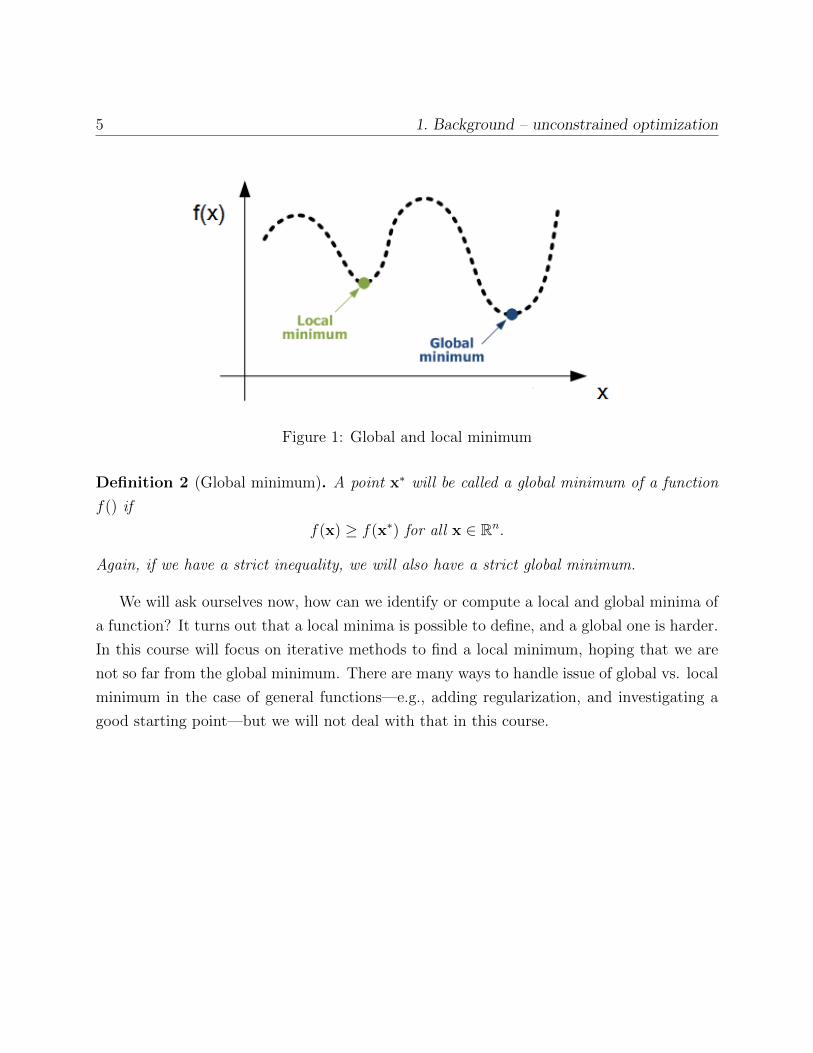
Figure 1: Global and local minimum
Definition 2 (Global minimum). A point x∗ will be called a global minimum of a function
f() if
f(x) ≥ f(x∗) for all x ∈ Rn.
Again, if we have a strict inequality, we will also have a strict global minimum.
We will ask ourselves now, how can we identify or compute a local and global minima of
a function? It turns out that a local minima is possible to define, and a global one is harder.
In this course will focus on iterative methods to find a local minimum, hoping that we are
not so far from the global minimum. There are many ways to handle issue of global vs. local
minimum in the case of general functions—e.g., adding regularization, and investigating a
good starting point—but we will not deal with that in this course.
6 1. Background – unconstrained optimization
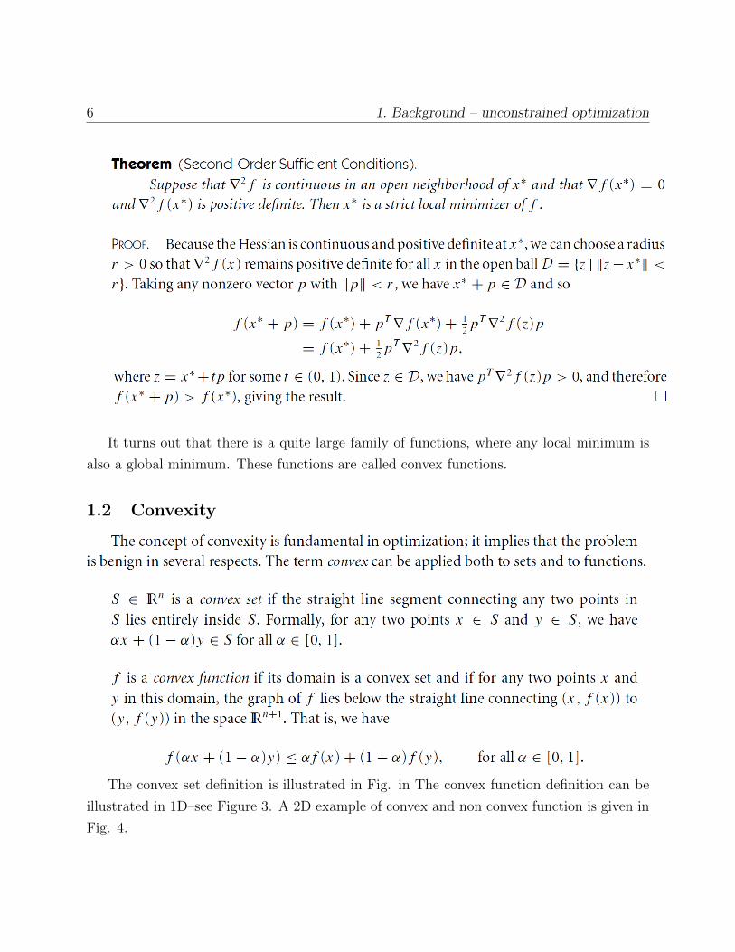
It turns out that there is a quite large family of functions, where any local minimum is
also a global minimum. These functions are called convex functions.
1.2 Convexity
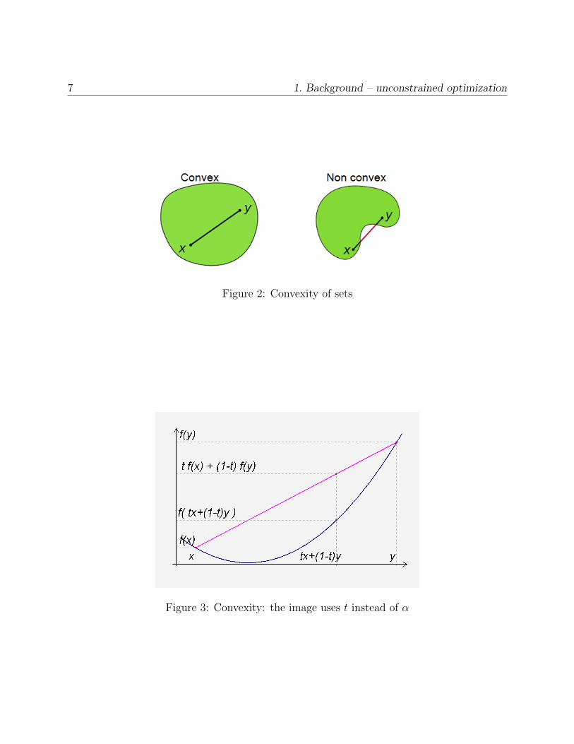
The convex set definition is illustrated in Fig. in The convex function definition can be
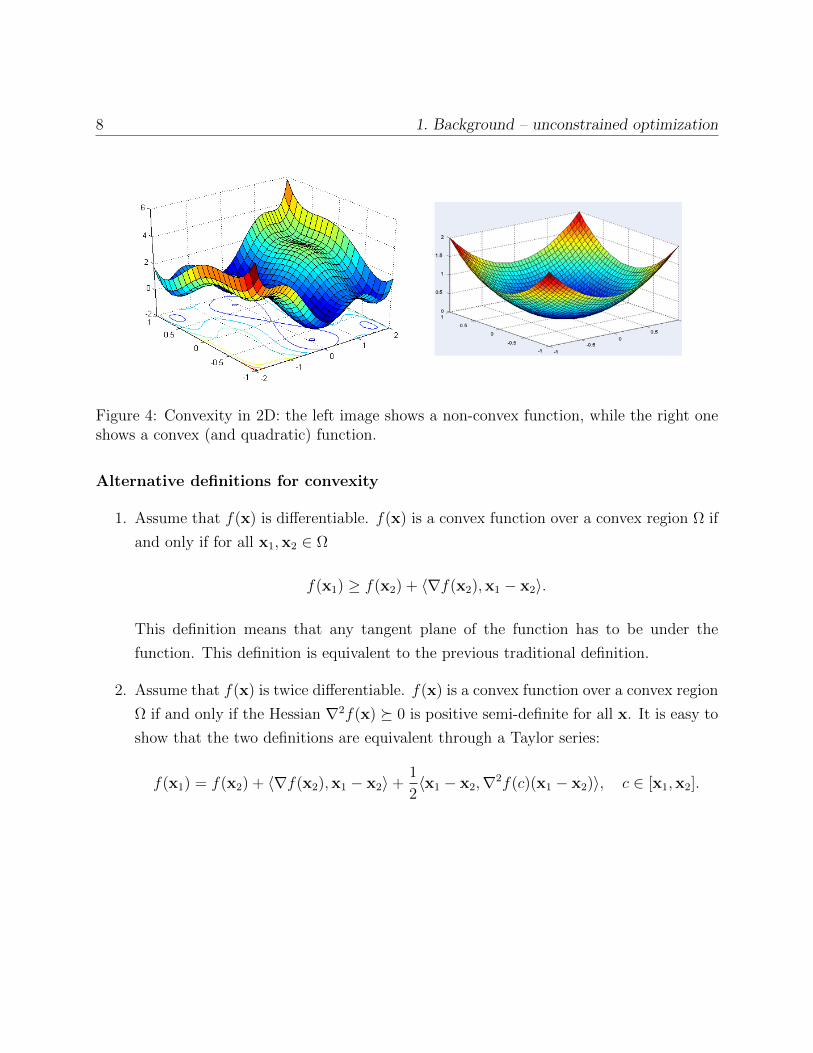
illustrated in 1D–see Figure 3. A 2D example of convex and non convex function is given in
Fig. 4.
7 1. Background – unconstrained optimization
Figure 2: Convexity of sets
Figure 3: Convexity: the image uses t instead of α
8 1. Background – unconstrained optimization
Figure 4: Convexity in 2D: the left image shows a non-convex function, while the right oneshows a convex (and quadratic) function.
Alternative definitions for convexity
1. Assume that f(x) is differentiable. f(x) is a convex function over a convex region Ω if
and only if for all x1,x2 ∈ Ω
f(x1) ≥ f(x2) + 〈∇f(x2),x1 − x2〉.
This definition means that any tangent plane of the function has to be under the
function. This definition is equivalent to the previous traditional definition.
2. Assume that f(x) is twice differentiable. f(x) is a convex function over a convex region
Ω if and only if the Hessian ∇2f(x) 0 is positive semi-definite for all x. It is easy to
show that the two definitions are equivalent through a Taylor series:
f(x1) = f(x2) + 〈∇f(x2),x1 − x2〉+1
2〈x1 − x2,∇2f(c)(x1 − x2)〉, c ∈ [x1,x2].
9 1. Background – unconstrained optimization
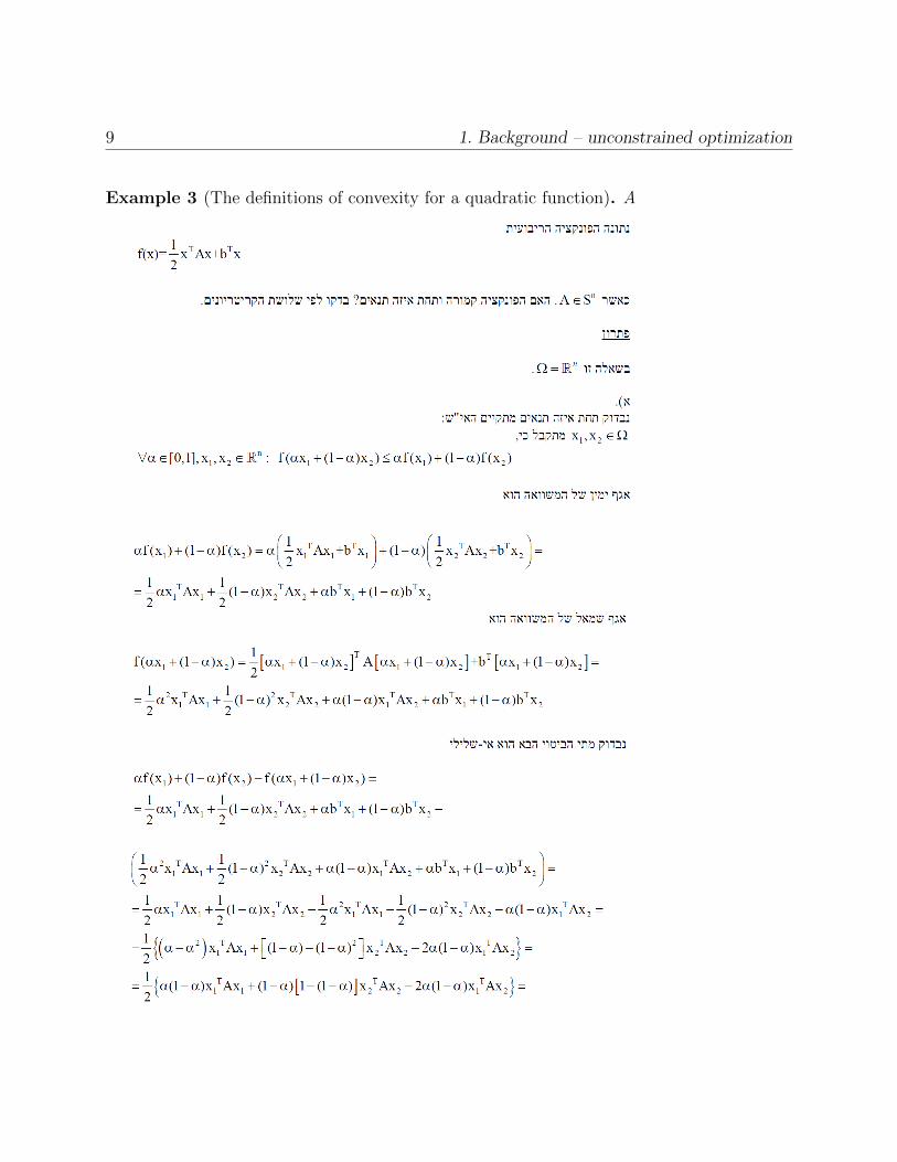
Example 3 (The definitions of convexity for a quadratic function). A
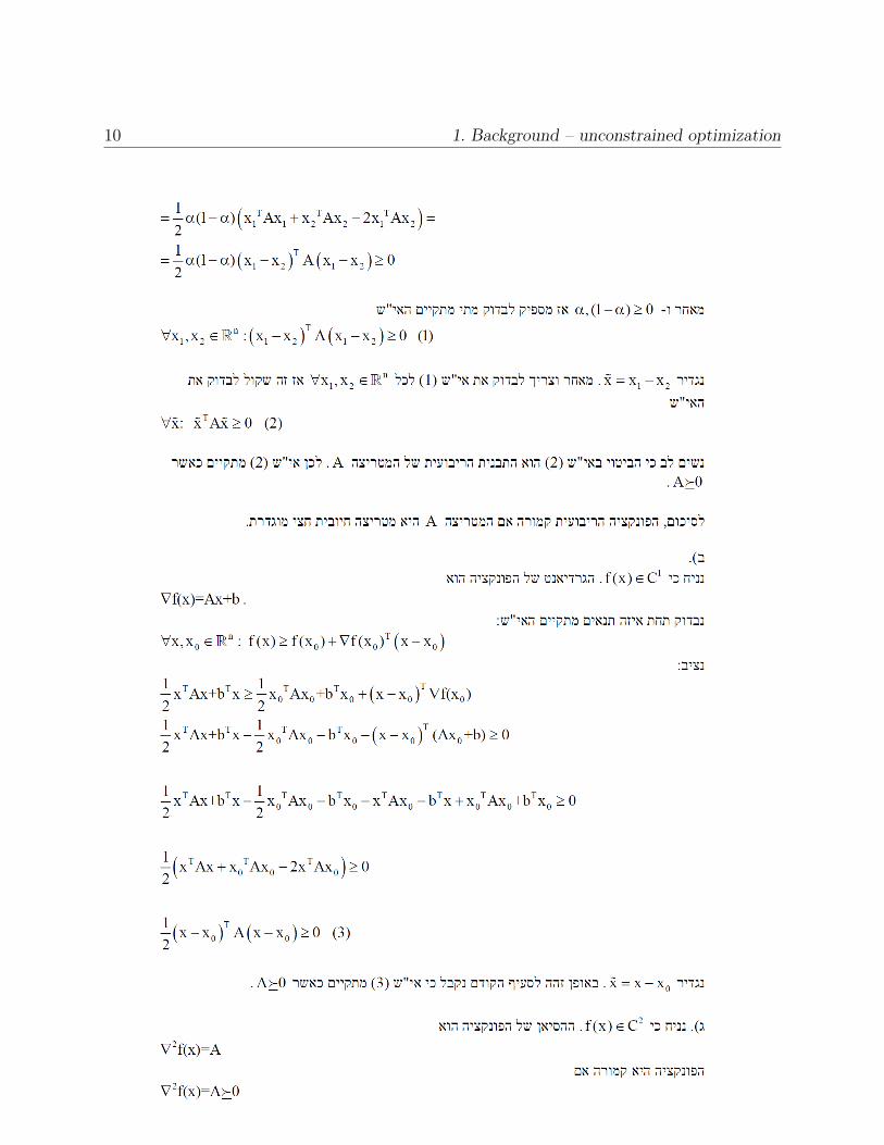
10 1. Background – unconstrained optimization
11 1. Background – unconstrained optimization
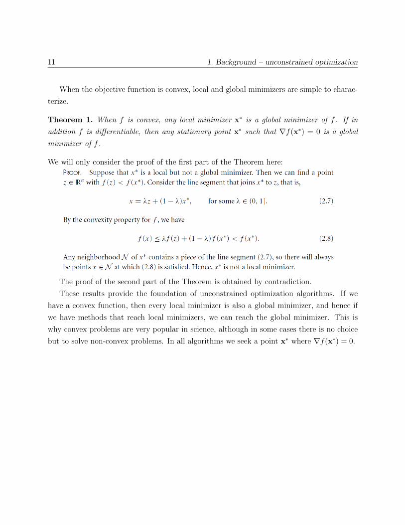
When the objective function is convex, local and global minimizers are simple to charac-
terize.
Theorem 1. When f is convex, any local minimizer x∗ is a global minimizer of f . If in
addition f is differentiable, then any stationary point x∗ such that ∇f(x∗) = 0 is a global
minimizer of f .
We will only consider the proof of the first part of the Theorem here:
The proof of the second part of the Theorem is obtained by contradiction.
These results provide the foundation of unconstrained optimization algorithms. If we
have a convex function, then every local minimizer is also a global minimizer, and hence if
we have methods that reach local minimizers, we can reach the global minimizer. This is
why convex problems are very popular in science, although in some cases there is no choice
but to solve non-convex problems. In all algorithms we seek a point x∗ where ∇f(x∗) = 0.
12 2. Iterative methods for unconstrained optimization
2 Iterative methods for unconstrained optimization
Just like linear systems, optimization can be carried out by iterative methods. Actually,
in optimization, it is usually not possible to directly find a minimum of a function, and so
iterative methods are much more essential in optimization than in numerical linear algebra.
On the other hand, we have learned about minimizing quadratic functions, which is equiv-
alent to solving linear systems. Since every function is locally approximated by a quadratic
function (and specifically near its minimum) everything we learned about iterative methods
for linear systems can be useful in the context of optimization.
2.1 Steepest descent (SD)
Earlier, we met the steepest descent method
x(k+1) = x(k) − α(k)∇f(x(k)),
which we analysed for positive definite linear systems Ax = b. In fact, we saw that if we
look at the equivalent quadratic minimization, then the matrix A has to be positive definite,
which means that the quadratic function f has to be convex (this does not mean that a
general f has to be convex for Steepest Descent to work). Just like quadratic (algebraic)
case, α(k) can be chosen sufficiently small, whether a constant α(k) = α or not, so that the
method converges to a local minimum. However, a more common way is to look at α(k) as
a step size, and choose it in some wise way.
2.2 A descent direction
In the method of SD, we chose the direction
dSD = −∇f(x(k)), (2)
as the most obvious choice for a descent direction (which requires a suitable step-size).
Among all the directions that we could choose from x(k), this is the one in which f decreases
most rapidly. To verify this claim, let us first define a descent direction: a direction in which
the value of f decreases. To define such a direction we use Taylor’s theorem. Let d be a
13 2. Iterative methods for unconstrained optimization
direction of norm 1 (‖d‖ = 1), and let α > 0 be a positive step size. We have:
f(x + αd) = f(x(k)) + α〈∇f,d〉+1
2α2〈d,∇2f(xk + td)d〉, t ∈ (0, α).
Now, for α > 0 sufficiently small, we will have that
f(x(k) + αd) < f(x(k)) ⇔ 〈∇f(x(k)),d〉 < 0, (3)
which is the condition for d to qualify as a descent direction.
Corollary 1. Any direction d = −M∇f such that M 0 is a descent direction.
It is easy to see that since we chose ‖d‖ = 1 we have
〈∇f,d〉 = ‖∇f‖‖d‖ cos(θ) = ‖∇f‖ cos(θ),
where θ is the angle between the vectors ∇f and d. to maximize the decrease in f we should
choose d such that cos(θ) = −1, which will be satisfied in θ = 180. That is the opposite
direction from the gradient, or, −∇f . This is the reason why (2) qualifies as the “steepest
descent” direction.
Interpretation of SD as quadratic minimization We will look at more general meth-
ods next, but first observe that steepest descent method (with a pre-defined step size α) can
be viewed as a step that minimizes the quadratic function that approximates f(x) around
x(k):
d(k)SD = arg min
d
f(x) + 〈∇f(x(k)),d〉+
1
2α〈d,d〉
= −α∇f(x(k)).
Then:
xk+1 = x(k) + d(k)SD = x(k) − α∇f(x(k)).
This derivation assumes that α is either constant or known a-priori. We will now see some
other methods that follow the same pattern, and later see a method for determining the step
length α through linesearch.
14 2. Iterative methods for unconstrained optimization
2.3 Newton, quasi-Newton
One of the most important methods outside of steepest descent is Newton’s method, which
is much more powerful than SD, but also may be more expensive. Recall again the Taylor
expansion
f(x(k) + ε) = f(x(k)) + 〈∇f(x(k)), ε〉+1
2〈ε,∇2f(x(k))ε〉+O(‖ε‖3). (4)
Now we choose the next step x(k+1) = x(k) + ε by a minimizing Eq. (4) without the O(‖ε‖3)
term with respect to ε. That is, the Newton direction dN is chosen by the following quadratic
minimization:
d(k)N = arg min
d
f(x) + 〈∇f(x(k)),d〉+
1
2〈d,∇2f(x(k))d〉
= −(∇f (x(k))−1)∇f(x(k)).
This minimization is similar to the one mentioned in SD, but now it has a ∇2f(x(k)) instead
of a matrix 1αI. This shows us that in SD we essentially approximate the real Hessian with
a scaled identity matrix.
The Newton procedure leads to a search direction
dN = −(∇2f(x(k)))−1∇f(x(k)),
which is the Newton’s direction. This is the best search direction that is practically used, and
it is relatively hard to obtain: first, the function f should be twice differentiable. Second,
one has to compute the Hessian matrix or at least know how to solve a non-trivial linear
system involving the Hessian matrix. This has to be computed at each iteration, which may
be costly. Solving the linear system can be done directly through an LU decomposition,
or iteratively using an appropriate method. If we choose a constant steplength, then one
can show that the best step-length for Newton’s method is asymptotically 1.0. However,
throughout the iterations it is better to perform a lineaserach over the direction dN to
guarantee the decreasing values of f(x(k)) and convergence.
It is important to note that the Newton’s method should be used with care. There is no
guarantee that d is a descent direction, or that the matrix (∇2f(x(k))) is invertible. If the
problem is convex and the Hessian is positive definite - we have nothing to worry about.
15 2. Iterative methods for unconstrained optimization
Quasi Newton methods Applying the Newton’s method is expensive. In Quasi-Newton
we approximate the Hessian by some matrix M(x(k)), and at each step minimize
d(k)QN = arg min
d
f(x) + 〈∇f(x(k)),d〉+
1
2〈d,M(x(k))d〉
= −(M(x(k))−1)∇f(x(k)). (5)
M can be chosen as diagonal, M = cI or M = diag(∇2f), which is easily invertible, or by
other ways. We will not go into this further in this course, but the limited memory Broyden-
Fletcher-Goldfarb-Shanno (LBFGS) method is one of the most popular quasi-Newton meth-
ods in the literature. It iteratively builds a low rank approximation of the Hessian from
previous search directions, which is somewhat similar to some Krylov methods that we’ve
seen earlier in this course (e.g. GMRES).
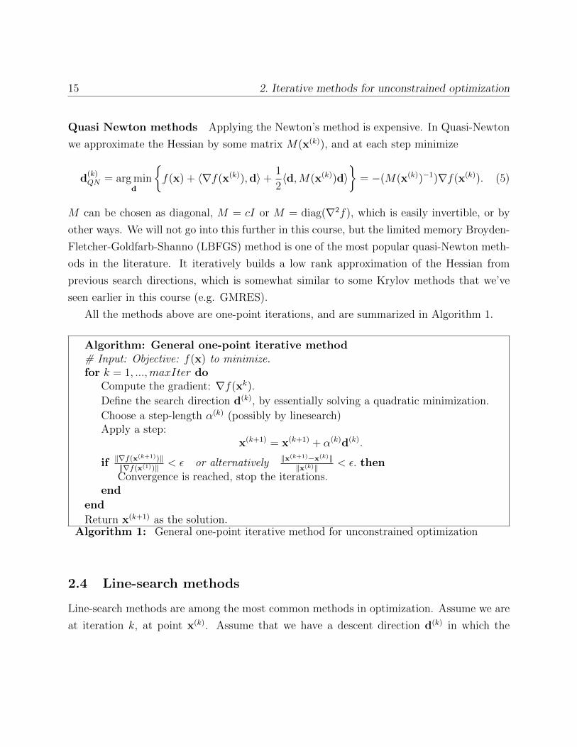
All the methods above are one-point iterations, and are summarized in Algorithm 1.
Algorithm: General one-point iterative method# Input: Objective: f(x) to minimize.for k = 1, ...,maxIter do
Compute the gradient: ∇f(xk).
Define the search direction d(k), by essentially solving a quadratic minimization.
Choose a step-length α(k) (possibly by linesearch)Apply a step:
x(k+1) = x(k+1) + α(k)d(k).
if ‖∇f(x(k+1))‖‖∇f(x(1))‖ < ε or alternatively ‖x(k+1)−x(k)‖
‖x(k)‖ < ε. thenConvergence is reached, stop the iterations.
end
end
Return x(k+1) as the solution.Algorithm 1: General one-point iterative method for unconstrained optimization
2.4 Line-search methods
Line-search methods are among the most common methods in optimization. Assume we are
at iteration k, at point x(k). Assume that we have a descent direction d(k) in which the
16 2. Iterative methods for unconstrained optimization
function decreases. Line-search methods performs
x(k+1) = x(k) + α(k)d(k) (6)
and choose α(k) such that f(x(k) + αd(k)) is exactly or approximately minimized for α. In
the quadratic SD case, we had a closed term that minimizes this linesearch.
When computing the step length α(k), we are essentially minimizing a one-dimensional
function
φ(α) = f(x(k) + αd(k)), α(k) = arg minα
φ(α)
with respect to α. All 1-D minimization methods can be used here, but we face a tradeoff.
We would like to choose α(k) to substantially reduce f , but at the same time we do not
want to spend too much time making the choice. In general, it is too expensive to identify
a minimizer, as it may require too many evaluations of the objective f . We assume here
that the computation of f(x(k) + αd(k)) is just as expensive as computing f(w) for some
arbitrary vector w. If this is not the case, we may be able to allow ourselves to invest more
iterations in minimizing φ(α). However, note that minimizing φ is only locally optimal (a
greedy choice), and there is no guarantee that an exact linesearch minimization is indeed
the right choice for the fastest convergence, not to mention the cost of doing that.
More practical strategies perform an inexact line search to identify a step length that
achieves adequate reductions in f at minimal cost. Typical line search algorithms try out
a sequence of candidate values for α, stopping to accept one of these values when certain
conditions are satisfied. Sophisticated line search algorithms can be quite complicated. We
now show a practical termination condition for the line search algorithm. We will later show,
using a simple quadratic example, that effective step lengths need not lie near the minimizers
of φ(α).
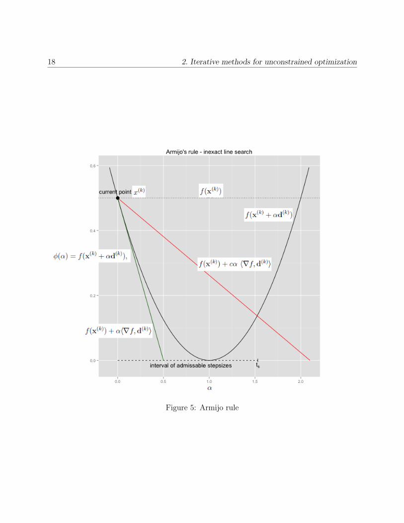
Backtracking line search using the Armijo condition We will now show one of the
most common line search algorithms, called “backtracking” line search, also known as the
Armijo rule. It involves starting with a relatively large estimate of the step size α, and
iteratively shrinking the step size (i.e., “backtracking”) until a sufficient decrease of the
objective function is observed. The motivation is to choose α(k) to be as large as possible
while having a sufficient decrease of the objective at the same time. We are not minimizing
17 2. Iterative methods for unconstrained optimization
φ. This is done by choosing α0 rather large, and choosing a decrease factor 0 < β < 1. We
will examine the values of φ(αj) for decreasing values αj = βjα0 (using j = 0, 1, 2, ...) until
the following condition is satisfied:
f(x(k) + αjd(k)) ≤ f(x(k)) + cαj〈∇f,d(k)〉. (7)
0 < c < 1 is usually chosen small (about 10−4), and β is usually chosen to be about 0.5. We
are guaranteed that such a point exists, because we assume that d(k) is a descent direction.
That is, we know that 〈∇f,d(k)〉 < 0, and using the Taylor theorem we have
f(x(k) + αd(k)) = f(x(k)) + α〈∇f,d(k)〉+O(α2‖d(k)‖2).
It is clear that for some α small enough we will have
f(x(k))− f(x(k) + αd(k)) = −α〈∇f,d(k)〉+O(α2‖d(k)‖2) > 0.
In our stopping rule we usually set c to be small, so we choose α to be relatively large.
Algorithm 2 summarizes the backtracking linesearch procedure. Common “upgrade” for this
procedure are
• Choose α0 for iteration k as 1βα(k−1) or 1
β2α(k−1).
• Instead of only reducing the αj’s, also try to enlarge them by αj+1 = 1βαj as long as
the Armijo condition is satisfied.
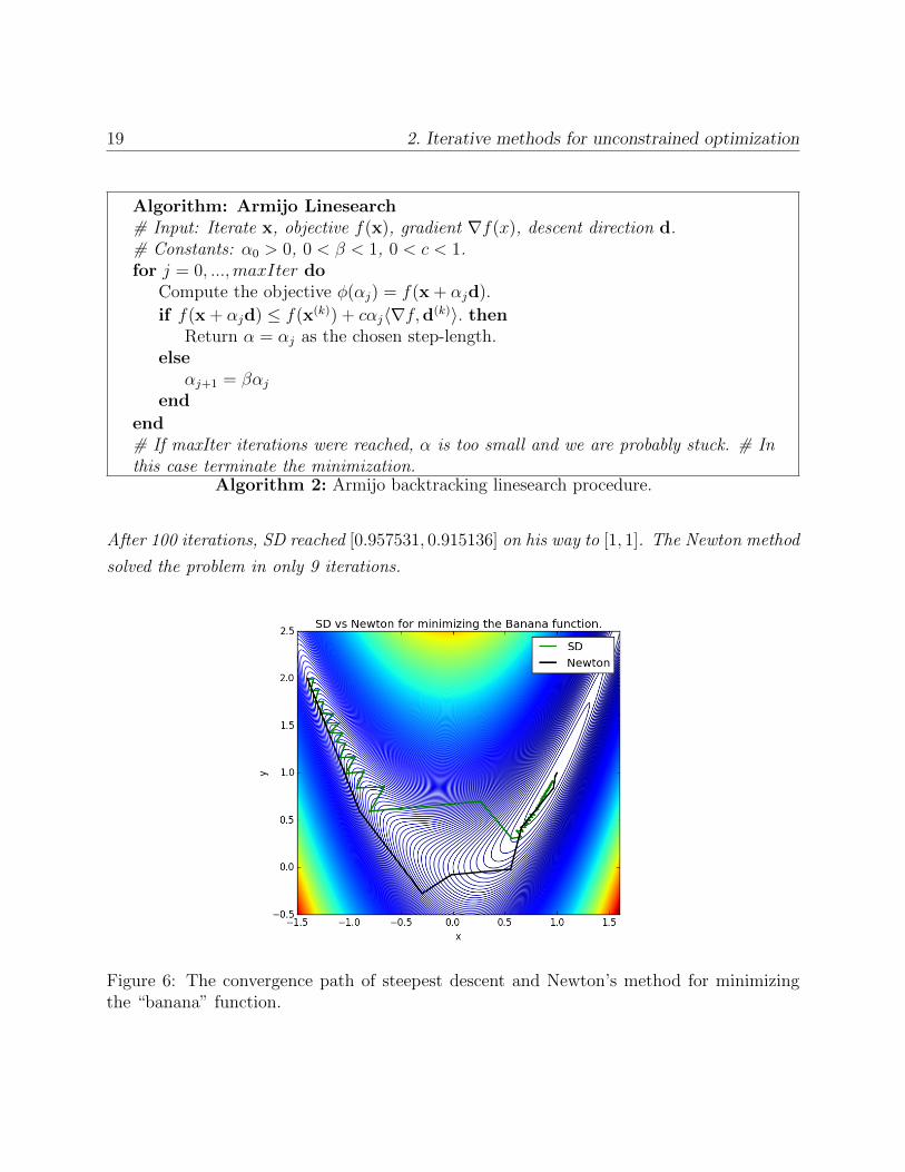
Example 4 (Newton vs. Steepest descent). We will now consider the minimization of the
Rosenbrock “banana” function f(x) = (a−x1)2 + b(x2−x21)2, where a, b are parameters that
determine the “difficulty” of the problem. Here we choose b = 5, and a = 1. The minimum
of this function is at [a, a2], where f = 0 (in our case it’s the point [1,1]).
The gradient and Hessian of this function are
∇f(x) =
[−4bx1(x2 − x2
1)− 2(a− x1)
2b(x2 − x21)
]∇2f(x) =
[−4b(x2 − x2
1) + 8bx21 + 2 −4bx1
−4bx2 2b
]
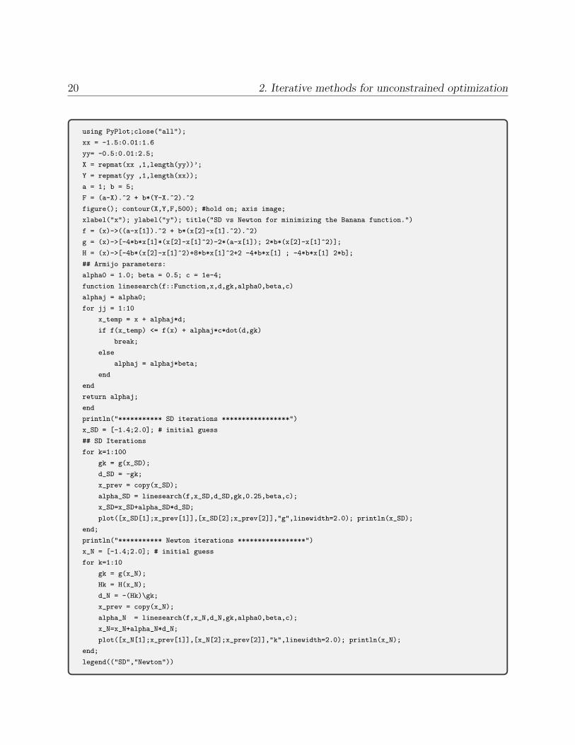
In the code below we apply the SD and Newton’s algorithms starting from the point [−1.4, 2].
18 2. Iterative methods for unconstrained optimization
Figure 5: Armijo rule
19 2. Iterative methods for unconstrained optimization
Algorithm: Armijo Linesearch# Input: Iterate x, objective f(x), gradient ∇f(x), descent direction d.# Constants: α0 > 0, 0 < β < 1, 0 < c < 1.for j = 0, ...,maxIter do
Compute the objective φ(αj) = f(x + αjd).
if f(x + αjd) ≤ f(x(k)) + cαj〈∇f,d(k)〉. thenReturn α = αj as the chosen step-length.
elseαj+1 = βαj
end
end# If maxIter iterations were reached, α is too small and we are probably stuck. # Inthis case terminate the minimization.
Algorithm 2: Armijo backtracking linesearch procedure.
After 100 iterations, SD reached [0.957531, 0.915136] on his way to [1, 1]. The Newton method
solved the problem in only 9 iterations.
Figure 6: The convergence path of steepest descent and Newton’s method for minimizingthe “banana” function.
20 2. Iterative methods for unconstrained optimization
using PyPlot;close("all");
xx = -1.5:0.01:1.6
yy= -0.5:0.01:2.5;
X = repmat(xx ,1,length(yy))’;
Y = repmat(yy ,1,length(xx));
a = 1; b = 5;
F = (a-X).^2 + b*(Y-X.^2).^2
figure(); contour(X,Y,F,500); #hold on; axis image;
xlabel("x"); ylabel("y"); title("SD vs Newton for minimizing the Banana function.")
f = (x)->((a-x[1]).^2 + b*(x[2]-x[1].^2).^2)
g = (x)->[-4*b*x[1]*(x[2]-x[1]^2)-2*(a-x[1]); 2*b*(x[2]-x[1]^2)];
H = (x)->[-4b*(x[2]-x[1]^2)+8*b*x[1]^2+2 -4*b*x[1] ; -4*b*x[1] 2*b];
## Armijo parameters:
alpha0 = 1.0; beta = 0.5; c = 1e-4;
function linesearch(f::Function,x,d,gk,alpha0,beta,c)
alphaj = alpha0;
for jj = 1:10
x_temp = x + alphaj*d;
if f(x_temp) <= f(x) + alphaj*c*dot(d,gk)
break;
else
alphaj = alphaj*beta;
end
end
return alphaj;
end
println("*********** SD iterations *****************")
x_SD = [-1.4;2.0]; # initial guess
## SD Iterations
for k=1:100
gk = g(x_SD);
d_SD = -gk;
x_prev = copy(x_SD);
alpha_SD = linesearch(f,x_SD,d_SD,gk,0.25,beta,c);
x_SD=x_SD+alpha_SD*d_SD;
plot([x_SD[1];x_prev[1]],[x_SD[2];x_prev[2]],"g",linewidth=2.0); println(x_SD);
end;
println("*********** Newton iterations *****************")
x_N = [-1.4;2.0]; # initial guess
for k=1:10
gk = g(x_N);
Hk = H(x_N);
d_N = -(Hk)\gk;
x_prev = copy(x_N);
alpha_N = linesearch(f,x_N,d_N,gk,alpha0,beta,c);
x_N=x_N+alpha_N*d_N;
plot([x_N[1];x_prev[1]],[x_N[2];x_prev[2]],"k",linewidth=2.0); println(x_N);
end;
legend(("SD","Newton"))
21 2. Iterative methods for unconstrained optimization
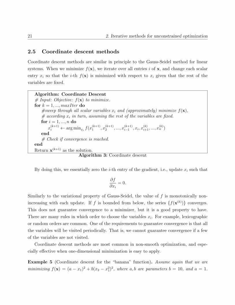
2.5 Coordinate descent methods
Coordinate descent methods are similar in principle to the Gauss-Seidel method for linear
systems. When we minimize f(x), we iterate over all entries i of x, and change each scalar
entry xi so that the i-th f(x) is minimized with respect to xi given that the rest of the
variables are fixed.
Algorithm: Coordinate Descent# Input: Objective: f(x) to minimize.for k = 1, ...,maxIter do
#sweep through all scalar variables xi and (approximately) minimize f(x),# according xi in turn, assuming the rest of the variables are fixed.for i = 1, ..., n do
x(k+1)i ← arg minxi f(x
(k+1)1 , x
(k+1)2 , ..., x
(k+1)i−1 , xi, x
(k)i+1, ..., x
(k)n )
end# Check if convergence is reached.
end
Return x(k+1) as the solution.Algorithm 3: Coordinate descent
By doing this, we essentially zero the i-th entry of the gradient, i.e., update xi such that
∂f
∂xi= 0.
Similarly to the variational property of Gauss-Seidel, the value of f is monotonically non-
increasing with each update. If f is bounded from below, the series f(x(k)) converges.
This does not guarantee convergence to a minimizer, but it is a good property to have.
There are many rules in which order to choose the variables xi. For example, lexicographic
or random orders are common. One of the requirements to guarantee convergence is that all
the variables will be visited periodically. That is, we cannot guarantee convergence if a few
of the variables are not visited.
Coordinate descent methods are most common in non-smooth optimization, and espe-
cially effective when one-dimensional minimization is easy to apply.
Example 5 (Coordinate descent for the “banana” function). Assume again that we are
minimizing f(x) = (a − x1)2 + b(x2 − x21)2, where a, b are parameters b = 10, and a = 1.
22 2. Iterative methods for unconstrained optimization
We’ve seen that
∇f(x) =
[−4bx1(x2 − x2
1)− 2(a− x1)
2b(x2 − x21)
],
and in coordinate descent we’re solving each of these equations in turn. We start with the
second variable, because the updates regarding the second variable are easy to define (assuming
b 6= 0)∂f
∂x2
= 2b(x2 − x21) = 0⇒ x2 = x2
1.
For the first variable, we have
∂f
∂x1
= −4bx1(x2 − x21)− 2(a− x1) = 0⇒ x1 =?[No closed form solution]
This time there is no closed form solution to the problem, and in fact there may be more
than one minimum point here. A common option in such cases is to apply a one-dimensional
Newton step for x1:
xnew1 = x1 − αf ′x1f ′′x1
= x1 − α−4bx1(x2 − x2
1)− 2(a− x1)
−4b(x2 − x21) + 8bx2
1 + 2
where α is obtained by linesearch with respect to minimizing f(x1 + αd1, x2) and d1 is the
Newton search direction for x1.
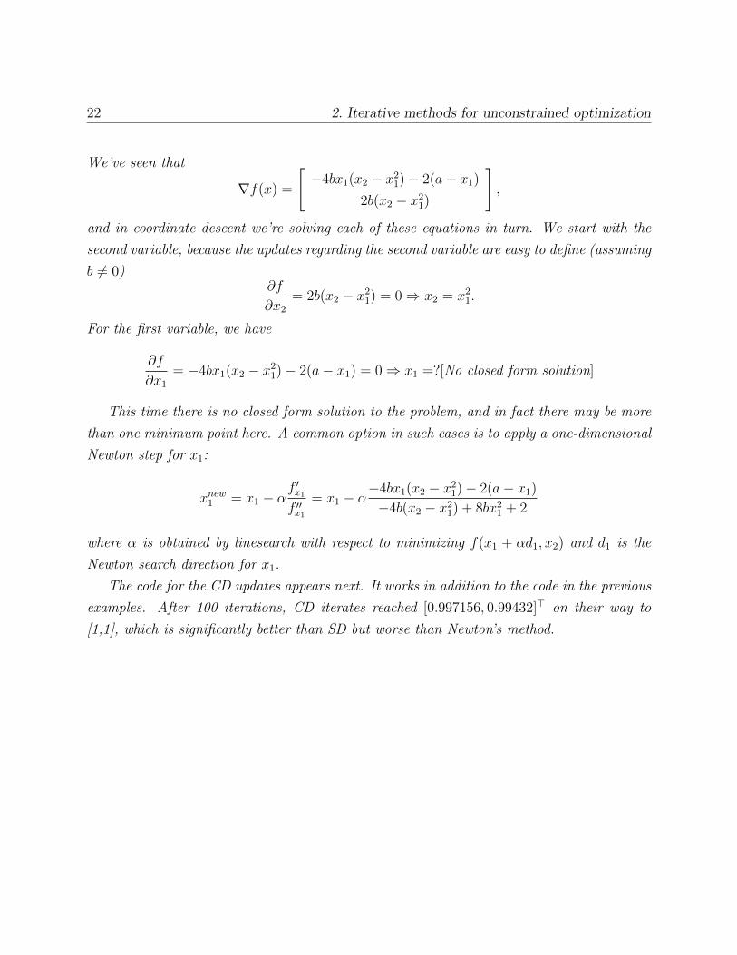
The code for the CD updates appears next. It works in addition to the code in the previous
examples. After 100 iterations, CD iterates reached [0.997156, 0.99432]> on their way to
[1,1], which is significantly better than SD but worse than Newton’s method.
23 2. Iterative methods for unconstrained optimization
Figure 7: The convergence path of the coordinate descent method for minimizing the “ba-nana” function.
## CD Iterations (this code comes in addition to the first section of code in the previous example)
x_CD = [-1.4;2.0];
println("*********** Newton *****************")
for k=1:100
# first variable Newton update:
gk = -4*b*x_CD[1]*(x_CD[2]-x_CD[1]^2)-2*(a-x_CD[1]); # This is g[1]
Hk = -4*b*(x_CD[2]-x_CD[1]^2)+8*b*x_CD[1]^2+2; # This is H[1,1]
d_1 = -gk/Hk; ## Hk is a scalar
f1 = (x)->((a-x).^2 + b*(x_CD[2]-x.^2).^2) # f1 accepts a scalar.
x_prev = copy(x_CD);
alpha_1 = linesearch(f1,x_CD[1],d_1,gk,alpha0,beta,c);
x_CD[1] = x_CD[1]+alpha_1*d_1;
# second variable update
x_CD[2] = x_CD[1]^2;
plot([x_CD[1];x_prev[1]],[x_CD[2];x_prev[2]],"k",linewidth=2.0); println(x_CD);
end;
2.6 Non-linear Conjugate Gradient methods
Earlier we’ve seen the Conjugate Gradient methods for linear systems. This method has
a lot of nice properties and advantages. It turns out that the linear CG method can be
extended to non-linear unconstrained optimization. This extension has many variants, and
all of them reduce to the linear CG method when the function is quadratic. We will not
study these methods in this course, but they are quite efficient and worthy of considera-
24 2. Iterative methods for unconstrained optimization
tion. See https://en.wikipedia.org/wiki/Nonlinear_conjugate_gradient_method for
an intuitive explanation.
2.7 Inexact Newton Methods - Newton-PCG
In this approach we can utilize the power of the Newton method, if the dimension of the
problem is too large for an exact inversion of the Hessian matrix. There are other reasons
why it may not be possible or efficient, but they are usually application specific. In this
method, instead of solving the system
∇2f(x(k))d = −∇f(x(k))
directly, we apply an iterative method to solve it approximately. The common choice is Con-
jugate Gradients, either with or without a preconditioner M . This way, the nice properties
of the linear CG method are in place and the solution is rather fast. This method is suitable
for ill-conditioned problems, where a Hessian-vector product (that is necessary in CG) is
easy to apply. This method is usually better than Steepest Descent (if it is applicable),
becasue (1) the gradient has to be computed only a few times, and (2) the good properties
of linear CG. The method is often comparable in performance to non-linear CG, but is more
stable and understandable.
25 3. Constrained Optimization
3 Constrained Optimization
In this section we will see the constrained optimization theory. The theory is a bit deep and
we will see only a few of the main results in this course. A general formulation of constrained
optimization problems has the form
minx∈Rn
f(x) subject to
ceqj (x) = 0 j = 1, ...,meq
cieql (x) ≤ 0 l = 1, ...,mieq, (8)
where f , ceqj , and cieqj are all smooth functions. f(x), as before, is the objective that we wish
to minimize. ceqj (x) are equality constraints, and cieqj (x) are inequality constraints. We define
a feasible set to be the set of all points that satisfy the constraints:
Ω =x|ceqj (x) = 0, j = 1, ...,meq ; cieql (x) ≤ 0, l = 1, ...,mieq
.
We can write (8) compactly as minx∈Ω f(x). The focus in this section is to characterize the
solutions of (8). Recall that for unconstrained minimization we had the following sufficient
optimality condition: Any point x∗ at which ∇f(x∗) = 0 and ∇2f(x∗) is positive definite
is a strong local minimizer of f . Our goal now is to define similar optimality conditions to
constrained optimization problems.
We have seen already that global solutions are difficult to find even when there are no
constraints. The situation may be improved when we add constraints, since the feasible set
might exclude many of the local minima, and it may be easy to pick the global minimum
from those that remain. However, constraints can also make things much more difficult. As
an example, consider the problem
minx∈Rn‖x‖2 s.t. ‖x‖2
2 ≥ 1.
Without the constraint, this is a convex quadratic problem with unique minimizer x = 0.
When the constraint is added, any vector x with ‖x‖2 = 1 solves the problem. There are
infinitely many such vectors (hence, infinitely many local minima) whenever n ≥ 2.
Definitions of the different types of local solutions are simple extensions of the corre-
sponding definitions for the unconstrained case, except that now we restrict consideration
to the feasible points in the neighborhood of x∗. We have the following definition.
26 3. Constrained Optimization
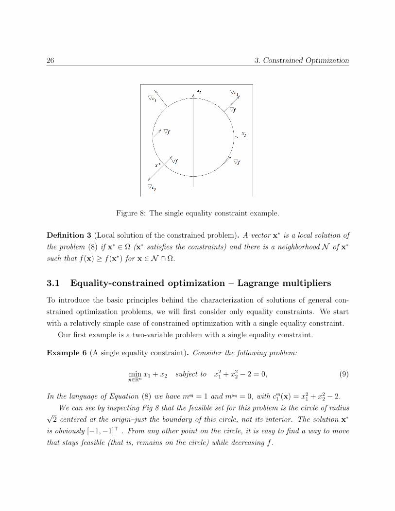
Figure 8: The single equality constraint example.
Definition 3 (Local solution of the constrained problem). A vector x∗ is a local solution of
the problem (8) if x∗ ∈ Ω (x∗ satisfies the constraints) and there is a neighborhood N of x∗
such that f(x) ≥ f(x∗) for x ∈ N ∩ Ω.
3.1 Equality-constrained optimization – Lagrange multipliers
To introduce the basic principles behind the characterization of solutions of general con-
strained optimization problems, we will first consider only equality constraints. We start
with a relatively simple case of constrained optimization with a single equality constraint.
Our first example is a two-variable problem with a single equality constraint.
Example 6 (A single equality constraint). Consider the following problem:
minx∈Rn
x1 + x2 subject to x21 + x2
2 − 2 = 0, (9)
In the language of Equation (8) we have meq = 1 and mieq = 0, with ceq1 (x) = x21 + x2
2 − 2.
We can see by inspecting Fig 8 that the feasible set for this problem is the circle of radius√2 centered at the origin–just the boundary of this circle, not its interior. The solution x∗
is obviously [−1,−1]> . From any other point on the circle, it is easy to find a way to move
that stays feasible (that is, remains on the circle) while decreasing f .
27 3. Constrained Optimization
We also see that at the optimal point x∗, the objective gradient ∇f is parallel to the
constraint gradient ∇ceq1 (x∗). In other words, there exists a scalar λ1 such that
∇f + λ1∇ceq1 (x∗) = 0, (10)
and in this particular case where ∇f = [1, 1]>, and ∇ceq1 = [2x1, 2x2]>, we have λ1 = 12, for
x = [−1,−1]>.
We can reach the same conclusion using the Taylor expansion. Assume a feasible point
x. To retain feasibility, any small movement in the direction d from x has to satisfy the
constraint
0 = ceq1 (x + d) ≈ ceq1 (x) + 〈∇ceq1 (x),d〉 = 〈∇ceq1 (x),d〉.
So any movement at the direction d from the point x has to satisfy
〈∇ceq1 (x),d〉 = 0. (11)
On the other hand, we have seen earlier than any descent direction has to satisfy
〈∇f(x),d〉 < 0 (12)
because f(x + d)− f(x) ≈ 〈∇f(x),d〉.If there exists a direction d, satisfying (11)-(12), then we can say that improvement in f
is possible under the constraints. It follows that a necessary condition for optimality for our
problem is that there is not a direction d satisfying both (11)-(12). The only way that such
a direction cannot exist is if ∇f(x) and ∇ceq1 (x) are parallel, otherwise
d =
(I − 1
∇ceq1 (x)>∇ceq1 (x)∇ceq1 (x)∇ceq1 (x)>
)∇f(x),
is a descent direction, which satisfies the constraints at least at first order. To eliminate this
option we will demand that there is no such direction, which also means that
1
∇ceq1 (x)>∇ceq1 (x)∇ceq1 (x)∇ceq1 (x)>∇f(x) = ∇f(x).
28 3. Constrained Optimization
Looking at the right hand side of the equation above as a least squares solution of
λ1 = arg minλ‖∇c1λ−∇f‖2
2,
that is because: λ1 = 1∇ceq1 (x)>∇ceq1 (x)
∇ceq1 (x)>∇f(x) we conclude that the least squares mini-
mization above must be satisfied with a value of 0. It means that there exists a λ1 satisfying
(10).
Because of the reasoning above, we can “pack” the objective and its equality constraints
into one function called the Lagrangian function
L(x, λ1) = f(x) + λ1ceq
1 (x),
for which ∇xL = ∇xf(x) + λ1∇xceq
1 (x). Hence, at the solution x∗ there exists a scalar λ1
such that
∇xL(x∗, λ∗1) = 0.
Note that the condition ∇λ1L = 0 provides the constraint ceq1 (x) = 0. This observation
suggests that we can search for solutions of the equality-constrained problem by searching for
stationary points of the Lagrangian function. The scalar quantity λ1 is called a Lagrange
multiplier for the constraint ceq1 (x) = 0. The condition above appears to be necessary for an
optimal solution of the problem, but it is clearly not sufficient. For example, the point [1, 1]>
also satisfies it in our example, but it is the maximum of the function under the constraint.
Back to our general equality constrained problem, which we write as
minx∈Rn
f(x) subject to ceq(x) = 0, (13)
where ceq(x) : Rn → Rmeqis the constraints vector function, that is
ceq(x) =
ceq1 (x)
ceq2 (x)...
ceqmeq (x)
= 0.
To obtain the optimality conditions we will first make an assumption on a point x∗ regarding
29 3. Constrained Optimization
the constraints.
Definition 4 (LICQ for equality constrained optimization). Given the point x∗, we say that
the linear independence constraint qualification (LICQ) holds if the set of constraint gradients
∇ceqi is linearly independent, or equivalently, if the Jacobian of the constraints vector Jeq(x∗)
is a full-rank matrix.
Note that if this condition holds, none of the constraint gradients can be zero. This
assumption comes to simplify our derivations and is not really necessary from a practical
point of view. For example, it breaks if we write one of the constraints twice. This clearly
should have any practical influence on our ability to solve problems.
A generalization of our conclusion from the previous example is as follows. In order for
x∗ to be a stationary point, there shouldn’t be a direction d such that 〈∇f(x),d〉 < 0 and
〈∇ceqi (x),d〉 = 0 for i = 1, ...,meq . In other words, the gradient cannot have a component
that is orthogonal to all the constraints’ gradients. More explicitly let
Jeq =
− ∇ceq1 (x) −− ∇ceq2 (x) −
...
− ∇ceqmeq (x) −
.
be the Jacobian of the constraints, the demand above will happen only if (similarly to the
1D case) the orthogonal projection of the gradient on the span of its rows is zero (dropping
the eq notation):
(I − JT (JJT )−1J
)∇f = 0⇒ min
λ‖JTλ−∇f‖2
2 = 0.
This also means that ∇f(x) is a linear combination of Jeq ’s rows, and we get the condition:
∇f(x) +meq∑i=1
λi∇ceqi (x) = ∇f(x) + (Jeq)>λ = 0.
Consequently, given an equality constrained problem (13), we write its Lagrangian function
as
L(x,λ) = f(x) + λ>ceq(x),
30 3. Constrained Optimization
where the vector λ ∈ Rmeqis the Lagrange multipliers vector.
Theorem 2 (Lagrange multipliers for equality constrained minimization). Let x∗ be a local
solution of (13), in particular satisfying the equality constraints ceq(x∗) = 0, and the LICQ
condition. Then there exists a unique vector λ∗ ∈ Rmeqcalled the Lagrange multipliers vector
which satisfies
∇xL(x∗,λ∗) = ∇f(x∗) + (Jeq)>λ∗ = 0.
We will not prove this theorem, but note that ∇λL(x∗,λ∗) = 0 ⇒ ceq(x∗) = 0, which
allows us to formulate a method for solving equality constrained optimization.
Back to our example of a single equality constraint
minx∈Rn
x1 + x2 subject to x21 + x2
2 − 2 = 0. (14)
The Lagrangian of this method is L(x, λ1) = x1 + x2 + λ1(x21 + x2
2 − 2) and the solution of
this problem is given by
∇L = 0⇒
1 + 2x1λ1 = 0
1 + 2x2λ1 = 0
x21 + x2
2 − 2 = 0
⇒
x1 = − 1
2λ1
x2 = − 12λ1
14λ21
+ 14λ21
= 2
⇒
λ1 = ±1
2
x1 = ∓1
x2 = ∓1
,
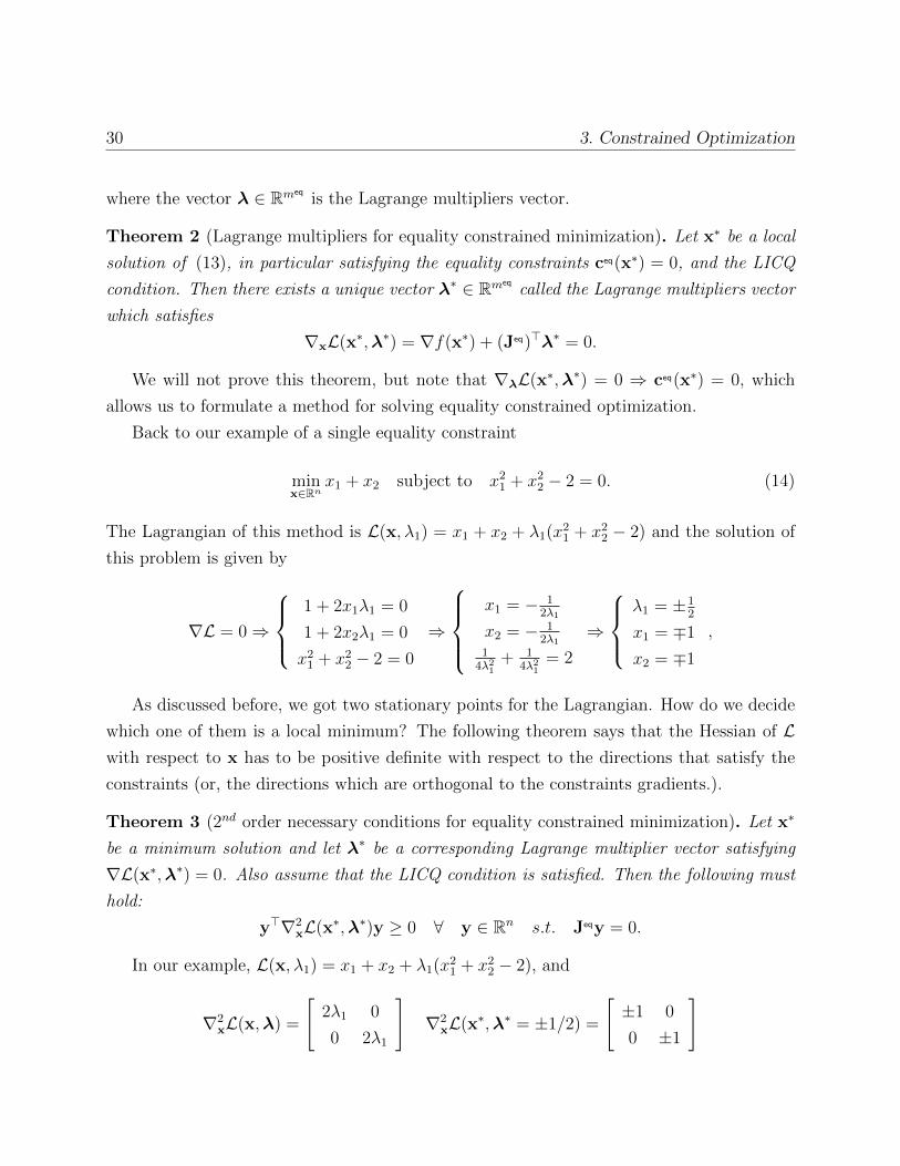
As discussed before, we got two stationary points for the Lagrangian. How do we decide
which one of them is a local minimum? The following theorem says that the Hessian of Lwith respect to x has to be positive definite with respect to the directions that satisfy the
constraints (or, the directions which are orthogonal to the constraints gradients.).
Theorem 3 (2nd order necessary conditions for equality constrained minimization). Let x∗
be a minimum solution and let λ∗ be a corresponding Lagrange multiplier vector satisfying
∇L(x∗,λ∗) = 0. Also assume that the LICQ condition is satisfied. Then the following must
hold:
y>∇2xL(x∗,λ∗)y ≥ 0 ∀ y ∈ Rn s.t. Jeqy = 0.
In our example, L(x, λ1) = x1 + x2 + λ1(x21 + x2
2 − 2), and
∇2xL(x,λ) =
[2λ1 0
0 2λ1
]∇2
xL(x∗,λ∗ = ±1/2) =
[±1 0
0 ±1
]
31 3. Constrained Optimization
It follows that the minimum is obtained at λ∗1 = 1/2 where ∇2xL(x∗,λ∗) = I 0. This
matrix is positive definite with respect to any vector, and in particular to those vectors that
are orthogonal to the constraint gradient. In the other point (λ1 = −1/2), we encounter the
case of the negative definite Hessian, and hence we have a local maximum.
3.2 The KKT optimality conditions for general constrained opti-
mization
Suppose now that we are considering the general case of constrained optimization, allowing
inequality constraints as well. Recall the following problem definition:
minx∈Rn
f(x) subject to
ceqj (x) = 0 j = 1, ...,meq
cieql (x) ≤ 0 l = 1, ...,mieq. (15)
It turns out that for this problem we should make a distinction between active inequality
constraints and inactive inequality constraints. Assume a local solution x∗. The active
constraints are those constraints for which cieql (x∗) = 0 and the inactive constraints are those
constraints for which cieql (x∗) < 0.
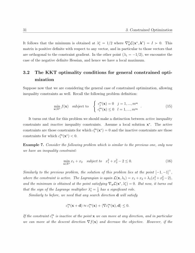
Example 7. Consider the following problem which is similar to the previous one, only now
we have an inequality constraint:
minx∈Rn
x1 + x2 subject to x21 + x2
2 − 2 ≤ 0. (16)
Similarly to the previous problem, the solution of this problem lies at the point [−1,−1]>,
where the constraint is active. The Lagrangian is again L(x, λ1) = x1 +x2 +λ1(x21 +x2
2− 2),
and the minimum is obtained at the point satisfying ∇xL(x∗, λ∗1) = 0. But now, it turns out
that the sign of the Lagrange multiplier λ∗1 = 12
has a significant role.
Similarly to before, we need that any search direction d will satisfy
cieq1 (x + d) ≈ cieq1 (x) + 〈∇cieq1 (x),d〉 ≤ 0.
If the constraint cieq1 is inactive at the point x we can move at any direction, and in particular
we can move at the descent direction ∇f(x) and decrease the objective. However, if the
32 3. Constrained Optimization
constraint is active, then cieq1 (x) = 0, and to satisfy the constraint we have the condition
〈∇cieq1 (x),d〉 ≤ 0. (17)
In order for d to be a legal descent direction it needs to satisfy both 〈∇f(x),d〉 < 0 and
(17). If we wish that d is not a descent direction, we need the inner products not to be both
negative. For this we must require that −∇f and ∇c1 will be at the same direction. That is:
∇f + λ1∇cieq1 (x∗) = 0,
with λ1 ≥ 0.
From the example above we learn that active inequality constraints act as equality
constraints but require the lagrange multiplier to be positive at stationary points. If we
have multiple inequality constraints, cieql (x) ≤ 0meq
l=1 , then we require that for a descent
direction d, each of them which is active will satisfy 〈∇cieql (x),d〉 ≤ 0, but if
∇f +∑
l active
λl∇cieql (x∗) = 0,
with λl ≥ 0, then
〈∇f(x),d〉+∑
l active
λl〈∇cieql (x∗),d〉 = 0,
and 〈∇f(x),d〉 ≥ 0 must hold. This means that d cannot be a descent direction under these
conditions.
We will now state the necessary conditions for a solution of a general constrained mini-
mization problem.
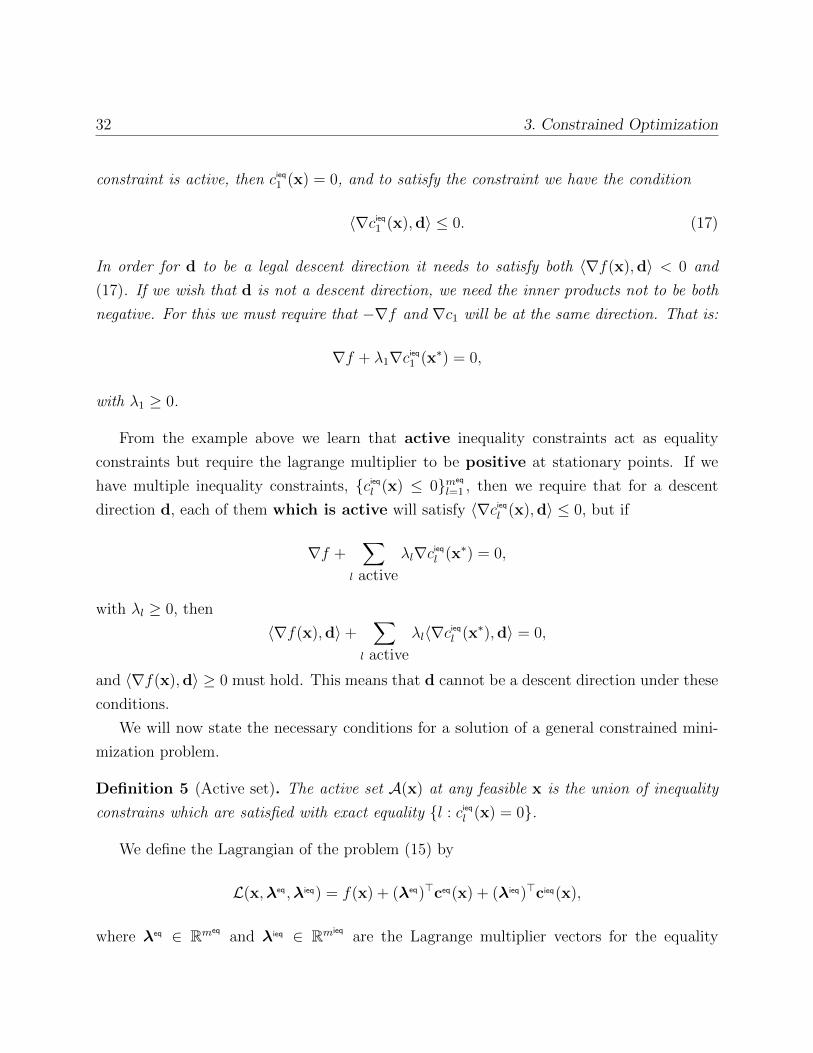
Definition 5 (Active set). The active set A(x) at any feasible x is the union of inequality
constrains which are satisfied with exact equality l : cieql (x) = 0.
We define the Lagrangian of the problem (15) by
L(x,λeq ,λieq) = f(x) + (λeq)>ceq(x) + (λieq)>cieq(x),
where λeq ∈ Rmeqand λieq ∈ Rmieq
are the Lagrange multiplier vectors for the equality
33 3. Constrained Optimization
and inequality constraints respectively. The next theorem states the first order necessary
conditions, known as the Karush-Kuhn-Tucker (KKT) conditions.
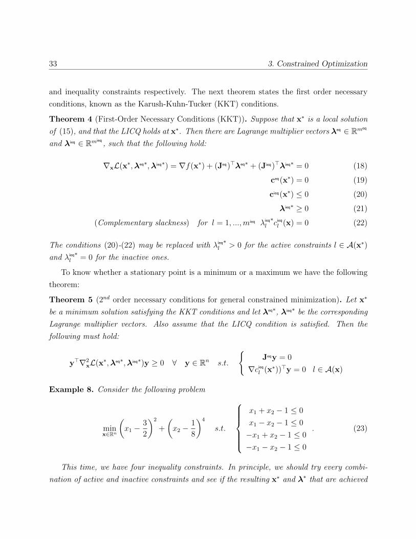
Theorem 4 (First-Order Necessary Conditions (KKT)). Suppose that x∗ is a local solution
of (15), and that the LICQ holds at x∗. Then there are Lagrange multiplier vectors λeq ∈ Rmeq
and λieq ∈ Rmieq, such that the following hold:
∇xL(x∗,λeq∗,λieq∗) = ∇f(x∗) + (Jeq)>λeq∗ + (Jieq)>λieq∗ = 0 (18)
ceq(x∗) = 0 (19)
cieq(x∗) ≤ 0 (20)
λieq∗ ≥ 0 (21)
(Complementary slackness) for l = 1, ...,mieq λieq∗l cieql (x) = 0 (22)
The conditions (20)-(22) may be replaced with λieq∗l > 0 for the active constraints l ∈ A(x∗)
and λieq∗l = 0 for the inactive ones.
To know whether a stationary point is a minimum or a maximum we have the following
theorem:
Theorem 5 (2nd order necessary conditions for general constrained minimization). Let x∗
be a minimum solution satisfying the KKT conditions and let λeq∗, λieq∗ be the corresponding
Lagrange multiplier vectors. Also assume that the LICQ condition is satisfied. Then the
following must hold:
y>∇2xL(x∗,λeq∗,λieq∗)y ≥ 0 ∀ y ∈ Rn s.t.
Jeqy = 0
∇cieql (x∗))>y = 0 l ∈ A(x)
Example 8. Consider the following problem
minx∈Rn
(x1 −
3
2
)2
+
(x2 −
1
8
)4
s.t.
x1 + x2 − 1 ≤ 0
x1 − x2 − 1 ≤ 0
−x1 + x2 − 1 ≤ 0
−x1 − x2 − 1 ≤ 0
. (23)
This time, we have four inequality constraints. In principle, we should try every combi-
nation of active and inactive constraints and see if the resulting x∗ and λ∗ that are achieved
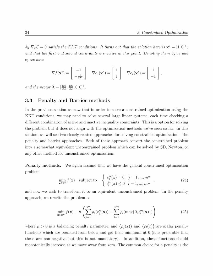
34 3. Constrained Optimization
by ∇xL = 0 satisfy the KKT conditions. It turns out that the solution here is x∗ = [1, 0]>,
and that the first and second constraints are active at this point. Denoting them by c1 and
c2 we have
∇f(x∗) =
[−1
− 1128
]∇c1(x∗) =
[1
1
]∇c2(x∗) =
[1
−1
],
and the vector λ = [129256, 127
256, 0, 0]>.
3.3 Penalty and Barrier methods
In the previous section we saw that in order to solve a constrained optimization using the
KKT conditions, we may need to solve several large linear systems, each time checking a
different combination of active and inactive inequality constraints. This is a option for solving
the problem but it does not align with the optimization methods we’ve seen so far. In this
section, we will see two closely related approaches for solving constrained optimization—the
penalty and barrier approaches. Both of these approach convert the constrained problem
into a somewhat equivalent unconstrained problem which can be solved by SD, Newton, or
any other method for unconstrained optimization.
Penalty methods. We again assume that we have the general constrained optimization
problem
minx∈Rn
f(x) subject to
ceqj (x) = 0 j = 1, ...,meq
cieql (x) ≤ 0 l = 1, ...,mieq, (24)
and now we wish to transform it to an equivalent unconstrained problem. In the penalty
approach, we rewrite the problem as
minx∈Rn
f(x) + µ
(meq∑j=1
ρj(ceq
j (x)) +mieq∑l=1
ρl(max0, cieql (x))
)(25)
where µ > 0 is a balancing penalty parameter, and ρj(x) and ρl(x) are scalar penalty
functions which are bounded from below and get their minimum at 0 (it is preferable that
these are non-negative but this is not mandatory). In addition, these functions should
monotonically increase as we move away from zero. The common choice for a penalty is the
35 3. Constrained Optimization
quadratic function ρ(x) = x2, which has a minimum at 0. Using this choice, if we set µ→∞then the solution of (25) will be equal to that of (24). We will focus on this choice in this
course.
The problem (25) is an unconstrained optimization problem which can be solved using the
methods we’ve learned to far. For ρ(x) = x2, however, it turns out that the problem becomes
more and more ill-conditioned as µ→∞, which makes standard first-order approaches like
SD and CD slow. Therefore, in practice we will have a continuation strategy where we solve
the problem for iteratively increasing values of the penalty µ. That is we will define
µ0 < µ1 < ... <∞
and iteratively solve the problem for each of those µ′s, each time using the previous solution
as an initial guess for the next problem. We will stop when µ is large enough such that the
constraints are reasonably fulfilled. That is, for our largest value of µ, it may be that for
example one of the equality constraints satisfies c(x∗) = ε. Whether ε is small enough or
not will depend on the application that yielded the optimization problem.
Remark 1. Another popular choice for a penalty is the exact penalty function ρ(x) = |x|(absolute value). It is popular because unlike the quadratic function, the constraints will be
exactly fulfilled for some moderate µ and not only for µ → ∞. The downside here is that
this function is non-smooth and significantly complicates the optimization process. We will
not consider this choice further in this chapter.
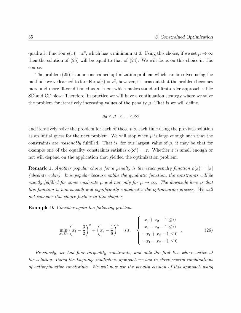
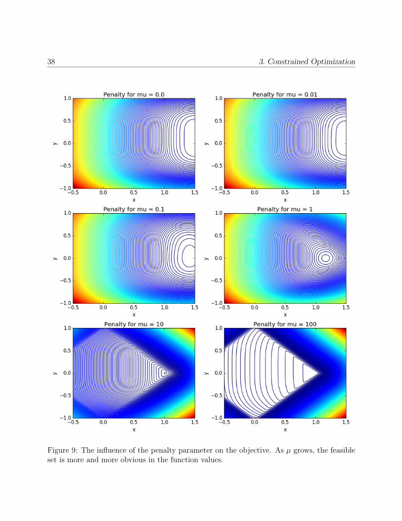
Example 9. Consider again the following problem
minx∈Rn
(x1 −
3
2
)2
+
(x2 −
1
8
)4
s.t.
x1 + x2 − 1 ≤ 0
x1 − x2 − 1 ≤ 0
−x1 + x2 − 1 ≤ 0
−x1 − x2 − 1 ≤ 0
. (26)
Previously, we had four inequality constraints, and only the first two where active at
the solution. Using the Lagrange multipliers approach we had to check several combinations
of active/inactive constraints. We will now use the penalty version of this approach using
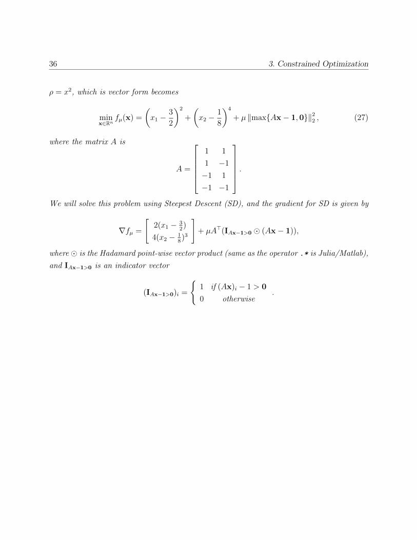
36 3. Constrained Optimization
ρ = x2, which is vector form becomes
minx∈Rn
fµ(x) =
(x1 −
3
2
)2
+
(x2 −
1
8
)4
+ µ ‖maxAx− 1,0‖22 , (27)
where the matrix A is
A =
1 1
1 −1
−1 1
−1 −1
.We will solve this problem using Steepest Descent (SD), and the gradient for SD is given by
∇fµ =
[2(x1 − 3
2)
4(x2 − 18)3
]+ µA>(IAx−1>0 (Ax− 1)),
where is the Hadamard point-wise vector product (same as the operator .* is Julia/Matlab),
and IAx−1>0 is an indicator vector
(IAx−1>0)i =
1 if (Ax)i − 1 > 0
0 otherwise.
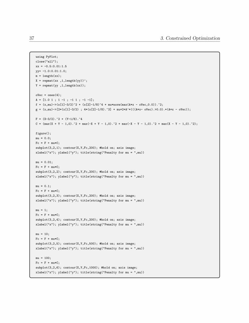
37 3. Constrained Optimization
using PyPlot;
close("all");
xx = -0.5:0.01:1.5
yy= -1.0:0.01:1.0;
m = length(xx);
X = repmat(xx ,1,length(yy))’;
Y = repmat(yy ,1,length(xx));
oVec = ones(4);
A = [1.0 1 ; 1 -1 ; -1 1 ; -1 -1];
f = (x,mu)->(x[1]-3/2)^2 + (x[2]-1/8)^4 + mu*norm(max(A*x - oVec,0.0)).^2;
g = (x,mu)->[2*(x[1]-3/2) ; 4*(x[2]-1/8).^3] + mu*2*A’*(((A*x- oVec).>0.0).*(A*x - oVec));
F = (X-3/2).^2 + (Y-1/8).^4
C = (max(X + Y - 1,0).^2 + max(-X + Y - 1,0).^2 + max(-X - Y - 1,0).^2 + max(X - Y - 1,0).^2);
figure();
mu = 0.0;
Fc = F + mu*C;
subplot(3,2,1); contour(X,Y,Fc,200); #hold on; axis image;
xlabel("x"); ylabel("y"); title(string("Penalty for mu = ",mu))
mu = 0.01;
Fc = F + mu*C;
subplot(3,2,2); contour(X,Y,Fc,200); #hold on; axis image;
xlabel("x"); ylabel("y"); title(string("Penalty for mu = ",mu))
mu = 0.1;
Fc = F + mu*C;
subplot(3,2,3); contour(X,Y,Fc,200); #hold on; axis image;
xlabel("x"); ylabel("y"); title(string("Penalty for mu = ",mu))
mu = 1;
Fc = F + mu*C;
subplot(3,2,4); contour(X,Y,Fc,200); #hold on; axis image;
xlabel("x"); ylabel("y"); title(string("Penalty for mu = ",mu))
mu = 10;
Fc = F + mu*C;
subplot(3,2,5); contour(X,Y,Fc,500); #hold on; axis image;
xlabel("x"); ylabel("y"); title(string("Penalty for mu = ",mu))
mu = 100;
Fc = F + mu*C;
subplot(3,2,6); contour(X,Y,Fc,1000); #hold on; axis image;
xlabel("x"); ylabel("y"); title(string("Penalty for mu = ",mu))
38 3. Constrained Optimization
Figure 9: The influence of the penalty parameter on the objective. As µ grows, the feasibleset is more and more obvious in the function values.
39 3. Constrained Optimization
## Armijo parameters:
alpha0 = 1.0; beta = 0.5; c = 1e-1;
## See the Armijo linesearch function in previous examples.
## Starting point
x_SD = [-0.5;0.8];
muVec = [0.1; 1.0 ; 10.0 ; 100.0]
fvals = []; cvals = [];figure();
## SD Iterations
for jmu = 1:length(muVec)
mu = muVec[jmu]
fmu = (x)->f(x,mu);
println("mu = ",mu)
Fc = F + mu*C;
subplot(2,2,jmu); contour(X,Y,Fc,1000); #hold on; axis image;
xlabel("x"); ylabel("y"); title(string("SD for mu = ",mu))
for k=1:50
gk = g(x_SD,mu);
if norm(gk) < 1e-3
break;
end
d_SD = -gk;
x_prev = copy(x_SD);
alpha_SD = linesearch(fmu,x_SD,d_SD,gk,0.5,beta,c);
x_SD=x_SD+alpha_SD*d_SD;
plot([x_SD[1];x_prev[1]],[x_SD[2];x_prev[2]],"g",linewidth=2.0);
println(x_SD,",",norm(gk),",",alpha_SD,",",f(x_SD,mu));
fvals = [fvals;f(x_SD,mu)];
cvals = [cvals;norm(max(A*x_SD - oVec,0.0))]
end;
end
figure();subplot(1,2,1);
plot(fvals);title("function values")
subplot(1,2,2);
semilogy(cvals,"*");title("Constraints violation values ||max(Ax-1,0)||")
Barrier methods We will now see the “sister” of the penalty method which offers a
different penalty approach. This approach is relevant only for inequality constraints, and is
used when we wish to require that the iterates will absolutely be inside the feasible domain.
The idea is to choose a “barrier” function that goes to∞ as we move towards the boundaries
of the feasible domain. Unlike the penalty approach we do not even define the objective
outside the feasible domain, and do not allow our iterates to go there.
There are two main “barrier functions”: the log-barrier function and the inverse-barrier
40 3. Constrained Optimization
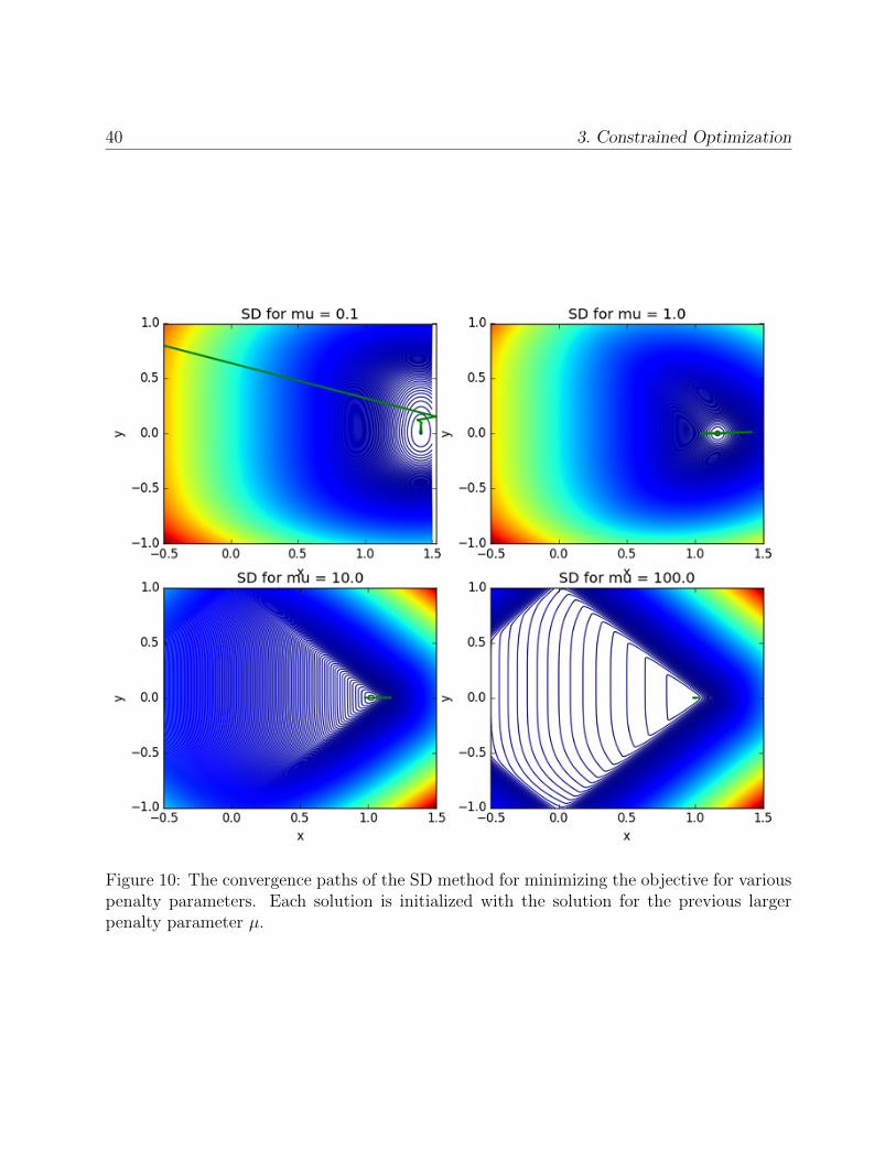
Figure 10: The convergence paths of the SD method for minimizing the objective for variouspenalty parameters. Each solution is initialized with the solution for the previous largerpenalty parameter µ.
41 3. Constrained Optimization
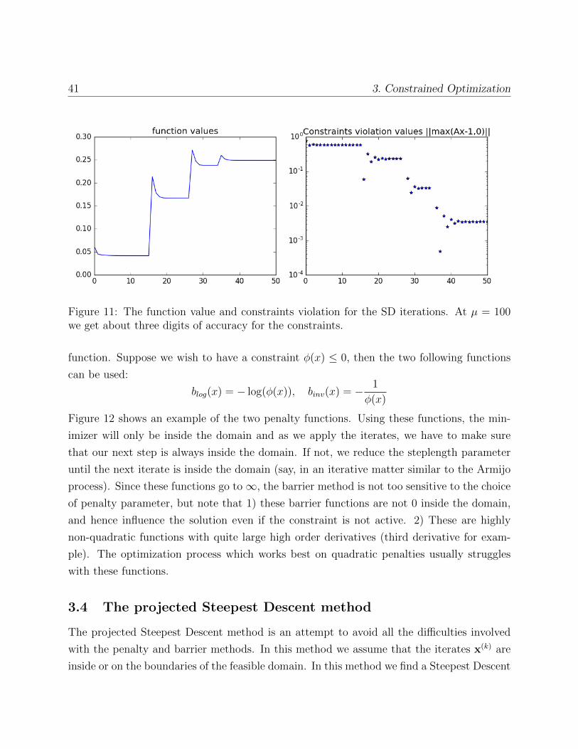
Figure 11: The function value and constraints violation for the SD iterations. At µ = 100we get about three digits of accuracy for the constraints.
function. Suppose we wish to have a constraint φ(x) ≤ 0, then the two following functions
can be used:
blog(x) = − log(φ(x)), binv(x) = − 1
φ(x)
Figure 12 shows an example of the two penalty functions. Using these functions, the min-
imizer will only be inside the domain and as we apply the iterates, we have to make sure
that our next step is always inside the domain. If not, we reduce the steplength parameter
until the next iterate is inside the domain (say, in an iterative matter similar to the Armijo
process). Since these functions go to∞, the barrier method is not too sensitive to the choice
of penalty parameter, but note that 1) these barrier functions are not 0 inside the domain,
and hence influence the solution even if the constraint is not active. 2) These are highly
non-quadratic functions with quite large high order derivatives (third derivative for exam-
ple). The optimization process which works best on quadratic penalties usually struggles
with these functions.
3.4 The projected Steepest Descent method
The projected Steepest Descent method is an attempt to avoid all the difficulties involved
with the penalty and barrier methods. In this method we assume that the iterates x(k) are
inside or on the boundaries of the feasible domain. In this method we find a Steepest Descent
42 3. Constrained Optimization
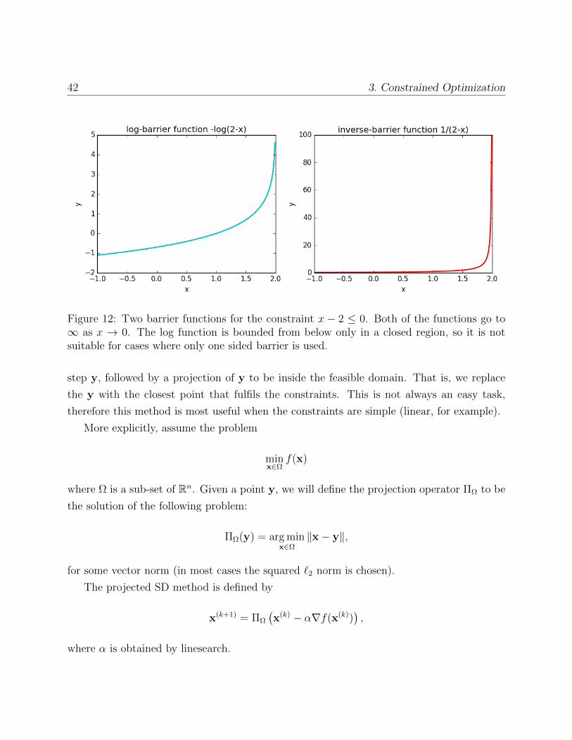
Figure 12: Two barrier functions for the constraint x − 2 ≤ 0. Both of the functions go to∞ as x → 0. The log function is bounded from below only in a closed region, so it is notsuitable for cases where only one sided barrier is used.
step y, followed by a projection of y to be inside the feasible domain. That is, we replace
the y with the closest point that fulfils the constraints. This is not always an easy task,
therefore this method is most useful when the constraints are simple (linear, for example).
More explicitly, assume the problem
minx∈Ω
f(x)
where Ω is a sub-set of Rn. Given a point y, we will define the projection operator ΠΩ to be
the solution of the following problem:
ΠΩ(y) = arg minx∈Ω
‖x− y‖,
for some vector norm (in most cases the squared `2 norm is chosen).
The projected SD method is defined by
x(k+1) = ΠΩ
(x(k) − α∇f(x(k))
),
where α is obtained by linesearch.
43 3. Constrained Optimization
Example 10. Define the projected steepest descent method for the linearly constrained min-
imization
minx∈Rn
f(x), subject to Ax = b,
assuming A ∈ Rm×n with m < n is full rank).
All we need to define is the projection operator with respect to some norm, and then set
x(k+1) = ΠΩ
(x(k) − α∇f(x(k))
). We will choose the squared `2 norm.
ΠΩ(y) = arg minx∈Rn
1
2‖x− y‖2
2, subject to Ax = b
The Lagrangian of the system is given by
L(x,λ) =1
2‖x− y‖2
2 + λ>(Ax− b).
To solve the problem we will solve the system
∇xL = x− y + A>λ = 0⇒ x∗ = y − A>λ.
The lagrange multiplier λ∗ will be defined by the constraint:
Ax∗ = b⇒ A(y − A>λ) = b⇒ λ∗ = (AA>)−1(Ay − b).
Here we see that we should invert AA> ∈ Rm×m, which is invertible because we assumed that
A is full rank. To get the final solution for the projection we set
x∗ = y − A>λ∗ = y − A>(AA>)−1(Ay − b).
Now we set y = x(k)−α∇f(x(k)), and assume that x(k) satisfies the constraint (Ax(k) = b):
x(k+1) = x(k) − α∇f(x(k))− A>(AA>)−1(A(x(k) − α∇f(x(k)))− b)
= x(k) − α(I − A>(AA>)−1A)∇f(x(k)).
This way we get the projected SD method. α is chosen by linesearch. The operator (I −A>(AA>)−1A) is called an orthogonal projection operator. Using this method, every step
44 3. Constrained Optimization
x(k+1) − x(k) will be in the null space of A, that is A(x(k+1) − x(k)) = 0.
Example 11. The box-constrained minimization
minx∈Rn
f(x), subject to a ≤ x ≤ b,
where the bound vectors satisfy: a < b.
This time, the constraints impose a very simple solution to the problem. The lagrangian
is given by
L(x,λ) =1
2‖x− y‖2
2 + λ>1 (x− b) + λ>2 (−x + a).
and its gradient is given by
∇xL(x,λ) = x− y + λ1 − λ2.
But here, there are active and inactive constraints that we need to incorporate. If no con-
straint is active we will get x∗ = y. The problem is separable, so if ai ≤ yi ≤ bi then we
can set x∗i = yi without breaking the constraint, and hence (λ∗1)i = (λ∗2)i = 0, because the
constraints are inactive. If yi < ai, then the lower bound constraint is active and the upper
bound is not. We set x∗i = ai and
x∗i − yi − (λ2)i = 0⇒ (λ∗2)i = ai − yi > 0.
We get a positive Lagrange multiplier, which is what needs to be. If yi > bi, then the upper
bound constraint is active and the lower bound is not. We set x∗i = bi and
x∗i − yi + (λ1)i = 0⇒ (λ∗1)i = yi − bi > 0.
Overall, the projected steepest descent step is given by:
z = x(k) − α∇f(x(k)), x(k+1)i =
ai zi < ai
bi zi > bi
zi otherwise
.
45 4. Robust statistics in least squares problems
4 Robust statistics in least squares problems
In many applications we are needed to recover some property out of given some data mea-
surements and (maybe) some additional information or prior knowledge. In most cases we
have noise or error in the measurements, which we assume to belong to some distribution.
The most common statistical tool that we have is Gaussian Distribution, which leads to least-
squares type problems. However, what if some of the measurements are really corrupted?
(these are called “outliers”).
Example 12 (Linear regression with outliers.). Suppose that you are given with m measure-
ments (xi, yi) and wish to find the line that defines yi given xi. That is, find scalars a, b
so that axi + b ≈ yi for all i in an optimal way. Previously, we used the `2 norm and got the
LS problem
mina,b
∑(axi + b− yi)2,
or
mina,b
∥∥∥∥∥∥∥∥∥∥
x1 1
x2 1...
...
xn 1
[a
b
]−
y1
y2
...
yn
∥∥∥∥∥∥∥∥∥∥
2
.
It turns out that since we are squaring the error, then the approximation is very sensitive
to points with large errors. Such points appear in many cases of “real data” and they severely
influence the approximated properties that we wish to learn on the system (a and b in our
case).
As an alternative, we may use a different distance measure, which is quadratic around 0
(to fit the Gaussian assumption) but it is linear as we move away from 0. The new function
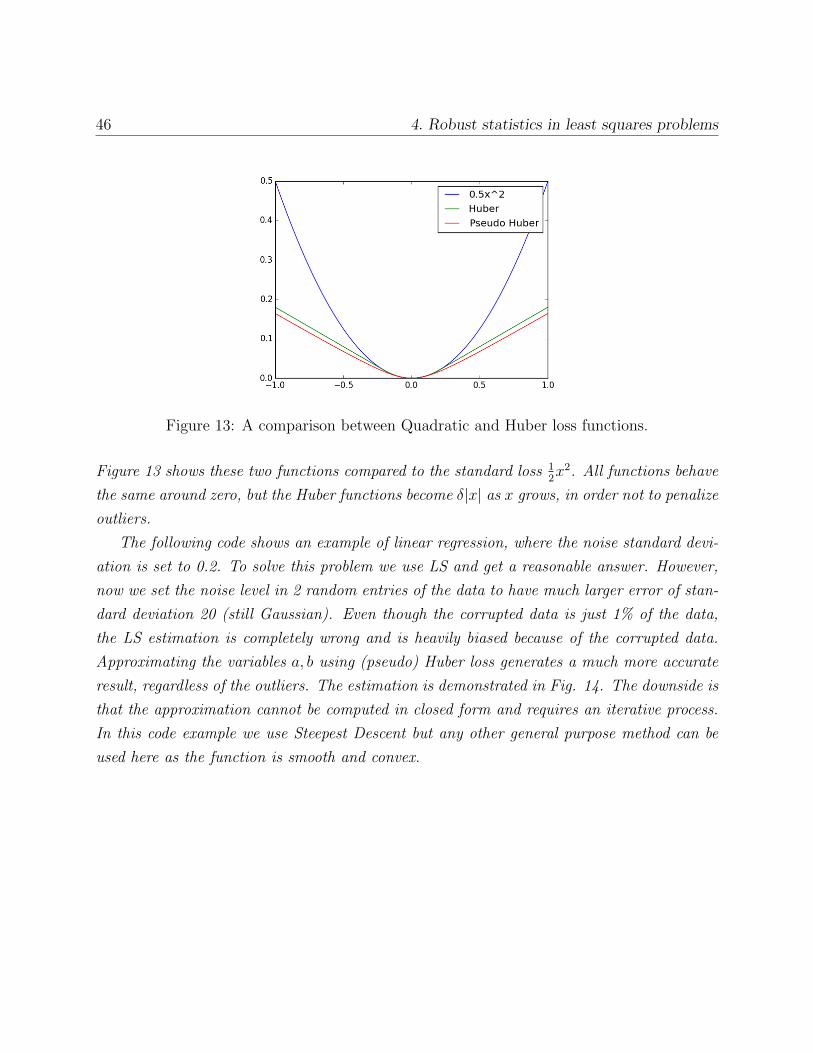
is called “Huber” loss function and is defined by
hδ(x) =
12x2 |x| ≤ δ
δ(|x| − 12δ) otherwise
.
This function is non smooth and is often replaced by the following “pseudo Huber” smooth
function
hδ(x) = δ√x2 + δ2 − δ2.
46 4. Robust statistics in least squares problems
Figure 13: A comparison between Quadratic and Huber loss functions.
Figure 13 shows these two functions compared to the standard loss 12x2. All functions behave
the same around zero, but the Huber functions become δ|x| as x grows, in order not to penalize
outliers.
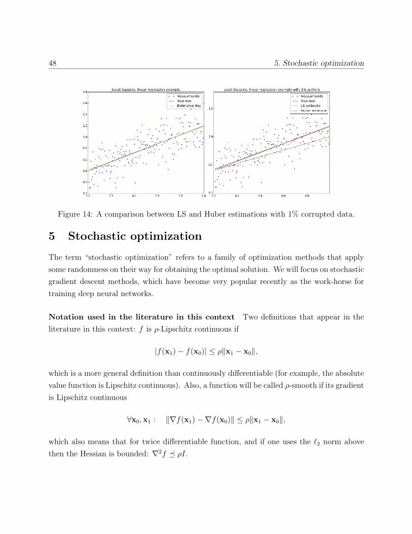
The following code shows an example of linear regression, where the noise standard devi-
ation is set to 0.2. To solve this problem we use LS and get a reasonable answer. However,
now we set the noise level in 2 random entries of the data to have much larger error of stan-
dard deviation 20 (still Gaussian). Even though the corrupted data is just 1% of the data,
the LS estimation is completely wrong and is heavily biased because of the corrupted data.
Approximating the variables a, b using (pseudo) Huber loss generates a much more accurate
result, regardless of the outliers. The estimation is demonstrated in Fig. 14. The downside is
that the approximation cannot be computed in closed form and requires an iterative process.
In this code example we use Steepest Descent but any other general purpose method can be
used here as the function is smooth and convex.
47 4. Robust statistics in least squares problems
x = linspace(0.01,1.0,200);a = 0.8;b = 0.4;sigma_noise = 0.2;
epsilon = sigma_noise*randn(length(x));
B = a.*x + b + epsilon;
A = [x ones(length(x))];
opt_ab = (A’*A) \ A’*B; # can be obtained using opt_ab = A\B;
figure();
subplot(1,2,1)
plot(x,B,".b");
plot(x,a*x + b,"-r");
plot(x,opt_ab[1]*x + opt_ab[2],"-g");
title("Least Squares: linear regression example");
legend(("Measurments","True line","Estimated line"));
corrupt_ind = randperm(200)[1:2];
epsilon[corrupt_ind] = 20.0*randn(length(corrupt_ind));
B = a.*x + b + epsilon;
opt_ab = (A’*A) \ A’*B; # can be obtained using opt_ab = A\B;
delta = sigma_noise;
hub = (x)->(r = A*x-B;f = sum(delta*(sqrt(x.^2 + delta^2)) - delta^2) ;return f;);
g_hub = (x)->(r = A*x-B; return A’*(delta*(r./sqrt(r.^2 + delta^2))); );
x_SD = [0.4;0.2];
println("*********** SD *****************")
## SD Iterations
for k=1:1000
gk = g_hub(x_SD);
d_SD = -gk;
x_prev = copy(x_SD);
alpha_SD = linesearch(hub,x_SD,d_SD,gk,1.0,beta,c); ## see linesearch() in previous examples.
x_SD=x_SD+alpha_SD*d_SD;
if norm(gk) < 1e-2
break;
end
end;
subplot(1,2,2)
plot(x,B,".b");
plot(x,a*x + b,"-r");
plot(x,opt_ab[1]*x + opt_ab[2],"-g");
plot(x,x_SD[1]*x + x_SD[2],"-k");
title("Least Squares: linear regression example with 1% outliers");
legend(("Measurments","True line","LS estimate","Huber estimate"));
48 5. Stochastic optimization
Figure 14: A comparison between LS and Huber estimations with 1% corrupted data.
5 Stochastic optimization
The term “stochastic optimization” refers to a family of optimization methods that apply
some randomness on their way for obtaining the optimal solution. We will focus on stochastic
gradient descent methods, which have become very popular recently as the work-horse for
training deep neural networks.
Notation used in the literature in this context Two definitions that appear in the
literature in this context: f is ρ-Lipschitz continuous if
|f(x1)− f(x0)| ≤ ρ‖x1 − x0‖,
which is a more general definition than continuously differentiable (for example, the absolute
value function is Lipschitz continuous). Also, a function will be called ρ-smooth if its gradient
is Lipschitz continuous
∀x0,x1 : ‖∇f(x1)−∇f(x0)‖ ≤ ρ‖x1 − x0‖,
which also means that for twice differentiable function, and if one uses the `2 norm above
then the Hessian is bounded: ∇2f ρI.
49 5. Stochastic optimization
A differentiable function f is µ-strongly convex if for every x,y:
f(y) ≥ f(x) +∇f(x)>(y − x) +µ
2‖y − x‖2 (28)
for some µ > 0.
A more general claim than strong convexity is the Polyak-Lojasiewicz (PL) inequality
which is quite useful for establishing linear convergence for a lot of algorithms:
∀x :1
2‖∇f(x)‖2 ≥ µ(f(x)− f(x∗)). (29)
(28)⇒(29) is obtained by minimizing both sides of (28) with respect to y.
Another more general claim that is achieved by (28) is
‖∇f(x)−∇f(y)‖ ≥ µ‖x− y‖.
This also means that if f is twice differentiable, then the Hessian’s eigenvalues are bounded
from below: ∇2f µI.
5.1 Stochastic Gradient descent
SGD was originally designed to save computations, but was actually saving computations in
very unique and limited cases. Later, it was shown that the power of SGD actually lies in
handling non-convex problems. Hence, we will distinguish between the performance of SGD
in solving convex problems versus solving (highly) non-convex problems.
To present SGD, we will revert to a notation that is more common in machine learning
applications: xi will be data samples (columns/rows of a matrix), and the vector w will be
a vector of unknown weights that we will optimize for (up until now the vector of unknowns
was denoted by x and the matrix rows/columns by ai).
Assume that you have some data ximi=1 to characterize. We can assume that ximi=1 is
drawn from some multivariate probabilistic distribution. Also assume that you can somehow
characterize this data by finding some vector of weights w ∈ Rn, which is found by minimizing
an objective according to some suitable model. Such optimization problem typically has the
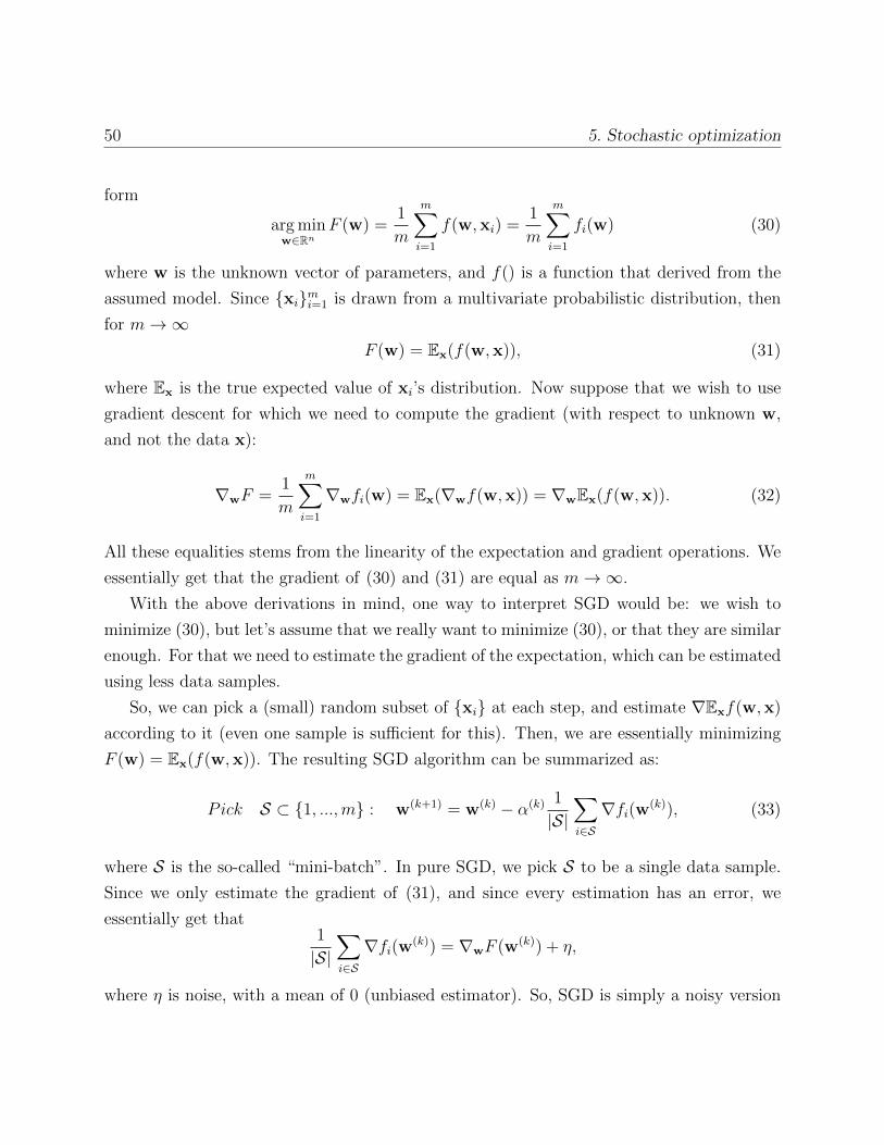
50 5. Stochastic optimization
form
arg minw∈Rn
F (w) =1
m
m∑i=1
f(w,xi) =1
m
m∑i=1
fi(w) (30)
where w is the unknown vector of parameters, and f() is a function that derived from the
assumed model. Since ximi=1 is drawn from a multivariate probabilistic distribution, then
for m→∞F (w) = Ex(f(w,x)), (31)
where Ex is the true expected value of xi’s distribution. Now suppose that we wish to use
gradient descent for which we need to compute the gradient (with respect to unknown w,
and not the data x):
∇wF =1
m
m∑i=1
∇wfi(w) = Ex(∇wf(w,x)) = ∇wEx(f(w,x)). (32)
All these equalities stems from the linearity of the expectation and gradient operations. We
essentially get that the gradient of (30) and (31) are equal as m→∞.
With the above derivations in mind, one way to interpret SGD would be: we wish to
minimize (30), but let’s assume that we really want to minimize (30), or that they are similar
enough. For that we need to estimate the gradient of the expectation, which can be estimated
using less data samples.
So, we can pick a (small) random subset of xi at each step, and estimate ∇Exf(w,x)
according to it (even one sample is sufficient for this). Then, we are essentially minimizing
F (w) = Ex(f(w,x)). The resulting SGD algorithm can be summarized as:
Pick S ⊂ 1, ...,m : w(k+1) = w(k) − α(k) 1
|S|∑i∈S
∇fi(w(k)), (33)
where S is the so-called “mini-batch”. In pure SGD, we pick S to be a single data sample.
Since we only estimate the gradient of (31), and since every estimation has an error, we
essentially get that1
|S|∑i∈S
∇fi(w(k)) = ∇wF (w(k)) + η,
where η is noise, with a mean of 0 (unbiased estimator). So, SGD is simply a noisy version
51 5. Stochastic optimization
of standard gradient descent if one look at minimizing (30). If we’re looking at minimizing
(31), then the noise in the gradient is inevitable anyway.
As in the previous cases, a key issue with SGD in (33) is the choice of the step-size
αk, which is also called the “learning rate”. Theory says that for convergence in convex
problems, we need to choose α(k) small and decaying (α(k) → 0), but still satisfy
limk→∞
k∑j=1
α(j) =∞.
Possible choices may be α(k) = 1k. In practice, α is often just chosen to be a sufficiently
small constant, or a set of constants for bunches of iterations, which is called “learning rate
scheduling”. For example, up to k = 100, α = 0.01, and from k = 100 on then α = 0.001.
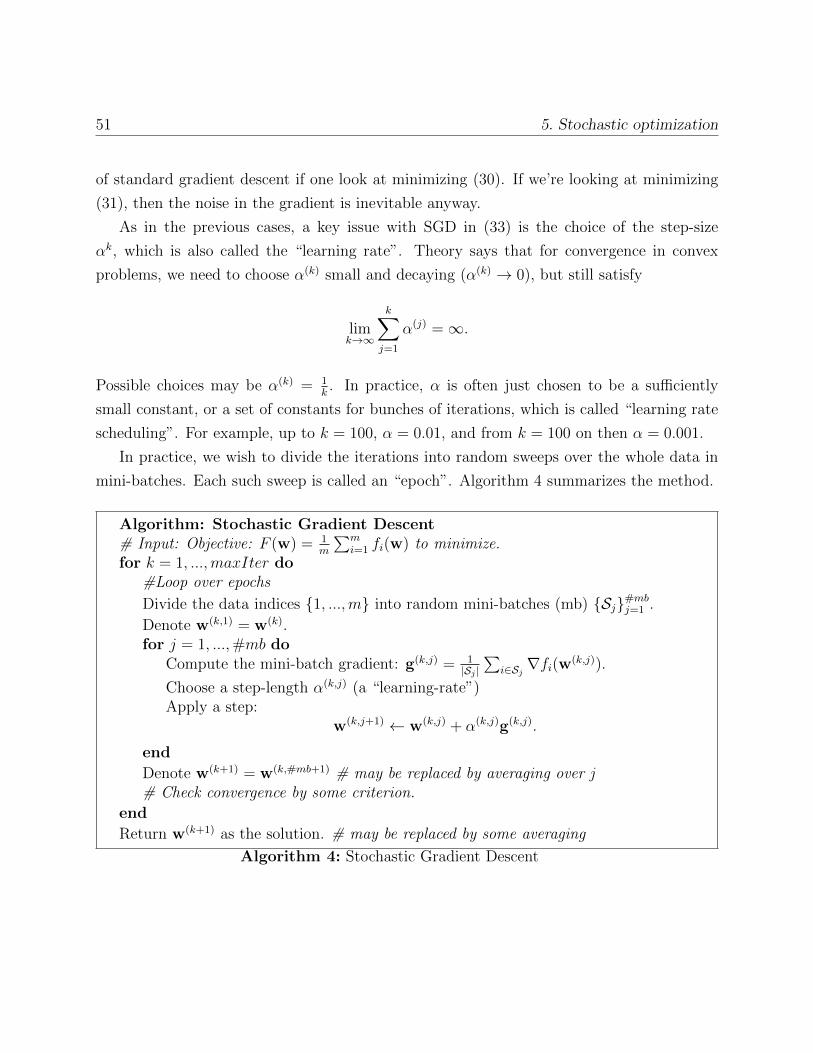
In practice, we wish to divide the iterations into random sweeps over the whole data in
mini-batches. Each such sweep is called an “epoch”. Algorithm 4 summarizes the method.
Algorithm: Stochastic Gradient Descent# Input: Objective: F (w) = 1
m
∑mi=1 fi(w) to minimize.
for k = 1, ...,maxIter do#Loop over epochs
Divide the data indices 1, ...,m into random mini-batches (mb) Sj#mbj=1 .
Denote w(k,1) = w(k).for j = 1, ...,#mb do
Compute the mini-batch gradient: g(k,j) = 1|Sj |∑
i∈Sj ∇fi(w(k,j)).
Choose a step-length α(k,j) (a “learning-rate”)Apply a step:
w(k,j+1) ← w(k,j) + α(k,j)g(k,j).
end
Denote w(k+1) = w(k,#mb+1) # may be replaced by averaging over j# Check convergence by some criterion.
end
Return w(k+1) as the solution. # may be replaced by some averaging
Algorithm 4: Stochastic Gradient Descent
52 5. Stochastic optimization
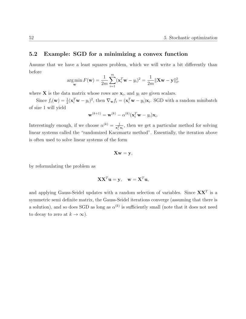
5.2 Example: SGD for a minimizing a convex function
Assume that we have a least squares problem, which we will write a bit differently than
before
arg minw
F (w) =1
2m
m∑i=1
(xTi w − yi)2 =1
2m‖Xw − y‖2
2,
where X is the data matrix whose rows are xi, and yi are given scalars.
Since fi(w) = 12(xTi w− yi)2, then ∇wfi = (xTi w− yi)xi. SGD with a random minibatch
of size 1 will yield
w(k+1) = w(k) − α(k)(xTi w − yi)xi.
Interestingly enough, if we choose α(k) = 1xTi xi
, then we get a particular method for solving
linear systems called the “randomized Kaczmartz method”. Essentially, the iteration above
is often used to solve linear systems of the form
Xw = y,
by reformulating the problem as
XXTu = y, w = XTu,
and applying Gauss-Seidel updates with a random selection of variables. Since XXT is a
symmetric semi definite matrix, the Gauss-Seidel iterations converge (assuming that there is
a solution), and so does SGD as long as α(k) is sufficiently small (note that it does not need
to decay to zero at k →∞).
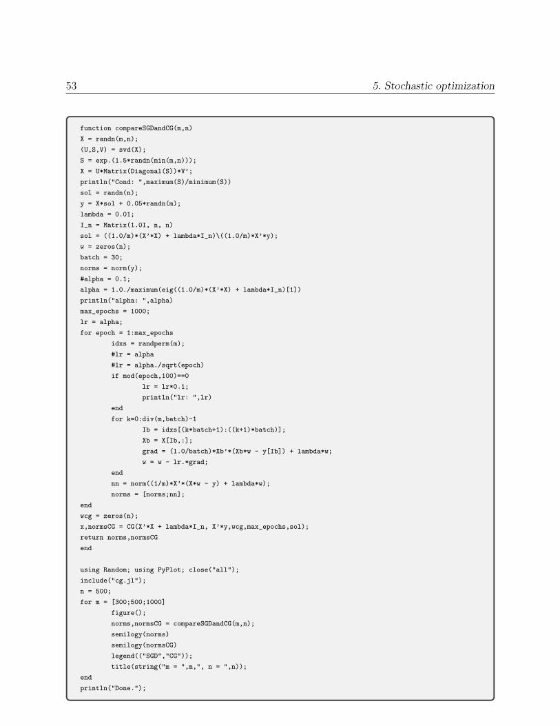
53 5. Stochastic optimization
function compareSGDandCG(m,n)
X = randn(m,n);
(U,S,V) = svd(X);
S = exp.(1.5*randn(min(m,n)));
X = U*Matrix(Diagonal(S))*V’;
println("Cond: ",maximum(S)/minimum(S))
sol = randn(n);
y = X*sol + 0.05*randn(m);
lambda = 0.01;
I_n = Matrix(1.0I, n, n)
sol = ((1.0/m)*(X’*X) + lambda*I_n)\((1.0/m)*X’*y);
w = zeros(n);
batch = 30;
norms = norm(y);
#alpha = 0.1;
alpha = 1.0./maximum(eig((1.0/m)*(X’*X) + lambda*I_n)[1])
println("alpha: ",alpha)
max_epochs = 1000;
lr = alpha;
for epoch = 1:max_epochs
idxs = randperm(m);
#lr = alpha
#lr = alpha./sqrt(epoch)
if mod(epoch,100)==0
lr = lr*0.1;
println("lr: ",lr)
end
for k=0:div(m,batch)-1
Ib = idxs[(k*batch+1):((k+1)*batch)];
Xb = X[Ib,:];
grad = (1.0/batch)*Xb’*(Xb*w - y[Ib]) + lambda*w;
w = w - lr.*grad;
end
nn = norm((1/m)*X’*(X*w - y) + lambda*w);
norms = [norms;nn];
end
wcg = zeros(n);
x,normsCG = CG(X’*X + lambda*I_n, X’*y,wcg,max_epochs,sol);
return norms,normsCG
end
using Random; using PyPlot; close("all");
include("cg.jl");
n = 500;
for m = [300;500;1000]
figure();
norms,normsCG = compareSGDandCG(m,n);
semilogy(norms)
semilogy(normsCG)
legend(("SGD","CG"));
title(string("m = ",m,", n = ",n));
end
println("Done.");
54 5. Stochastic optimization
5.3 Upgrades to SGD
SGD is the workhorse for many data science applications when the data dimension is much
higher than number of parameters, and when the problems are well conditioned. One way to
reduce the noise in SGD gradients is by averaging iterates/gradients or by re-scaling them.
Momentum One common way is by using the momentum strategy:
g(k) =1
|S|∑i∈S
∇fi(w(k))
m(k) = γm(k−1) + α(k)g(k)
w(k+1) = w(k) −m(k).
where m(0) is set to zero. The parameter γ is usually chosen to be between 0.5 and 0.9, and
generally, the learning rate α needs to be chosen smaller than in standard SGD. The momen-
tum drives the iterations in the direction of averaged gradients. One common pitfall of the
method is that the algorithm often fails to stop upon convergence (because the momentum
is not decaying to zero.)
AdaGrad Another approach is to rescale the gradients:
g(k) =1
|S|∑i∈S
∇fi(w(k))
v(k) = γv(k−1) + (1− γ)(g(k) g(k))
w(k+1) = w(k) − α(k) 1√v(k) v(k).
The symbol denotes the Hadamard (element-wise) product.
55 6. Minimization of Neural Networks for Classification
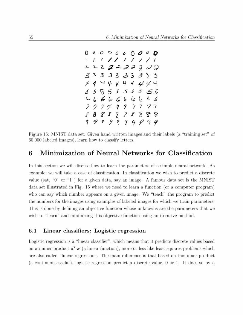
Figure 15: MNIST data set: Given hand written images and their labels (a “training set” of60,000 labeled images), learn how to classify letters.
6 Minimization of Neural Networks for Classification
In this section we will discuss how to learn the parameters of a simple neural network. As
example, we will take a case of classification. In classification we wish to predict a discrete
value (sat, “0” or “1”) for a given data, say an image. A famous data set is the MNIST
data set illustrated in Fig. 15 where we need to learn a function (or a computer program)
who can say which number appears on a given image. We “teach” the program to predict
the numbers for the images using examples of labeled images for which we train parameters.
This is done by defining an objective function whose unknowns are the parameters that we
wish to “learn” and minimizing this objective function using an iterative method.
6.1 Linear classifiers: Logistic regression
Logistic regression is a “linear classifier”, which means that it predicts discrete values based
on an inner product xTw (a linear function), more or less like least squares problems which
are also called “linear regression”. The main difference is that based on this inner product
(a continuous scalar), logistic regression predict a discrete value, 0 or 1. It does so by a
56 6. Minimization of Neural Networks for Classification
function called “logistic” or “sigmoid” function
σ(x>w) =1
1 + exp(−x>w)∈ [0, 1] (34)
The function σ(x>w) may be interpreted as the probability of x to be 0 or 1, given the
distribution parameter w. If we decide that
P (y = 1|x) = σ(x>w), P (y = 0|x) = 1− σ(x>w) (35)
then if σ(x>w) is close to 1, we will say that with high probability y = 1, and if not, then
y = 0. The labels can be chosen the other way around, and then w that we will learn will
just switch signs (−w will show probability 0 for label y = 1). We often refer to (34) as the
“(probabilistic) model” in which we classify the images.
In “supervised learning” we are given with labeled data (xi, yi)mi=1, such that xi ∈ Rn
and yi are discrete categorial labels (may be even “cat” and “dog”). In logistic regression,
we assume that we have only two labels (say, “cat” and “dog”) and we wish to train w based
on
F (w) = − 1
m
m∑i=1
(Iyi=dog log(σ(x>i w)) + Iyi=cat log(1− σ(x>i w))
)(36)
which is also the maximum likelyhood estimator of w that corresponds to the above prob-
ability. Iy=dog is an indicator function, that equals 1 if yi = dog and 0 otherwise. Once we
minimize this “loss” function and get the estimated parameters w∗, we can predict!. Given
a new image x, we compute σ(x>w). If the value is larger than 0.5, then we’ll predict that
x should be labeled as “dog”, and otherwise, as a “cat”.
We can write the objective in matrix-vector form. This way, it will be more efficient
to compute the objective in languages that are vectorized like Matlab, Python or R. Let
X ∈ Rn×m be the data matrix
X = [x1|x2|x3|...|xm],
and c1, c2 ∈ 0, 1m be the classes vectors as
c1 = [Iy1=dog, Iy2=dog, Iy3=dog, ..., Iym=dog]>, (37)
c2 = [Iy1=cat, Iy2=cat, Iy3=cat, ..., Iym=cat]>. (38)
57 6. Minimization of Neural Networks for Classification
The objective in (36) can be written in matrix form as
F (w) = − 1
m
(c>1 log
(σ(X>w)
)+ c>2 log
(1− σ(X>w)
)), (39)
where the scalar function σ operates on each vector component separately. We may also
write c2 = 1− c1, but keep it this way for the derivation of the softmax function.
Recall the following example:
Example 13. (The Jacobian of φ(x), where φ is a scalar function) Suppose that f = φ(x),
where φ : R → R is a scalar function, i.e., fi(x) = φ(xi). In this case the vector Taylor
expansion is just a vector of one dimensional expansions.
δf = φ(x + ε)− φi(x) ≈ diag(φ′(x))ε = diag(φ′(x))δx.
This means that J = diag(φ′(x)), which is a diagonal matrix such that Jii = φ′(xi).
6.1.1 Computing the gradient of logistic regression
First,
c>φ(X>(w + δw)) ≈ c>φ(X>w) + c>φ′(X>w)X>δw
and hence:
∇(c>φ(X>w)) = Xφ′(X>w)c (40)
Next, it is not hard to show that for (34) we have
σ′(t) = σ(t)(1− σ(t)), (log(σ(t)))′ = 1− σ(t), (log(1− σ(t)))′ = −σ(t)
In the first term of (39) we have φ1(X>w) = log(σ(X>w)), and for the second one we have
φ2(X>w) = log(1− σ(X>w)). Hence we get
58 6. Minimization of Neural Networks for Classification
∇wF = − 1
mX[φ′1(X>w)c1 + φ′2(X>w)c2
](41)
= − 1
mX[(1− σ(X>w))c1 − σ(X>w)c2
](42)
= − 1
mX[(1− σ(X>w))c1 − σ(X>w)(1− c1)
](43)
=1
mX[σ(X>w)− c1
](44)
The Hessian The Hessian of (39), which is also the Jacobian of (41), can be computed
using similar computations like (40). We get:
∇2F =1
mXDX>,
where D = σ′(X>w) = σ(X>w)(1 − σ(X>w)) is a diagonal matrix with only positive
numbers on the diagonal. Overall, the Hessian must be a semi definite matrix and hence,
the logistic regression objective is convex, and the strict convexity depends on whether the
matrix X is full rank (rank at least n) or not. It can be shown using Taylor series that
F (w + δw) =1
m‖X>δw − g‖2
D +O(‖δw‖3),
for some vector g, and hence, SGD will asymptotically behave as it behaves for least squares
problems, which we saw earlier.
6.1.2 Adding the bias
In some sense, the logistic regression model (34) separates the domain into two sides by a
linear function. If x>w > 0 the probability will come out larger than 0.5 and we will classify
x as “1”, while if x>w < 0, we will classify x as “0”. This means that we are separating the
entire Rn domain into two half-spaces by a linear function - all points x that lies above that
plain will be classified together. As we know, a plain (linear function) is usually defined by
x>w + b with a free parameter b ∈ R. Our case is no different, and in practice we need to
add b to the parameters of the logistic regression classifier. This term is called “bias”. To
keep all the derivations above, one can add the bias artificially by adding a pixel of 1 to any
59 6. Minimization of Neural Networks for Classification
image x, and to add one parameter to w.
6.2 Linear classifiers: Multinomial logistic (softmax) regression
The logistic regression objective was able to classify data images to two classes. What
happens if we have more than two?? Say, “dog”, “cat” and “horse” (in Fig 15 we have 10
labels)? The answer is the multinomial logistic regression which is also dubbed the “softmax”
function, which is a simple generalization of the logistic regression model to l labels.
Assume again that we have the labeled data (xi, yi)mi=1, where this time yi ∈ 1, ..., l.We will again use the (34) model, but now we will have l weight vectors wili=1. For each
image, we will have a probability of that image to be any of the labels (l probabilities). To
have them all sum to 1, we will define, somewhat similarly to (35)
P (y = j|x) =exp(x>wj)∑li=1 exp(x>wi)
∈ [0, 1]. (45)
The objective function can be written similarly to (39):
F (wklk=1) = − 1m
∑mi=1
(∑lk=1(ck)i log
(∑lj=1 exp(x>i wj)
−1
exp(x>i wk)
))(46)
= − 1m
∑lk=1 c>k log
(diag
∑lj=1 exp(X>wj)
−1
exp(X>wk)
). (47)
In softmax, one also need to add the bias terms, just like in logistic regression. We will have
one bias term for each label.
Remark 2. The diag...−1 term above is written this way so that the expression fulfils the
rule of linear algebra. Computing diag(v)−1u “as is” in the code for two large vectors v,u
is not efficient. To do so we may perform an element-wise division by. In code it is often
looks like u./v in most scientific languages (Matlab, Julia, etc.).
Computing extreme exponentials “safely” The terms above should sum to 1. How-
ever, as w>x is not bounded, the exponent may be computed by the computer as Inf (numer-
ical overflow), leaving the whole computation undetermined. As it happens, we can instead
60 6. Minimization of Neural Networks for Classification
computeexp(x>wj)∑li=1 exp(x>wi)
=exp(x>wj − η)∑li=1 exp(x>wi − η)
,
for some η, and in particular we can choose η = maxjx>wj, guaranteeing that the com-
putation will be performed without overflow.
6.2.1 Computing the gradient of softmax regression
The computation of the gradient is quite similar to the computation of the logistic regression.
We will use the following equality:
∂
∂tp
l∑k=1
ak log
(exp(tk)∑j exp(tj)
)= ap −
l∑k=1
akexp(tp)∑j exp(tj)
Using this equality and the fact that∑
k ck = 1, we get
∇wpF = − 1
mX
cp −l∑
k=1
diag
∑j
exp(X>wj)
−1
exp(XTwp)ck
= − 1
mX
cp − diag
∑j
exp(X>wj)
−1
exp(XTwp)l∑
k=1
ck
=
1
mX
diag
∑j
exp(X>wj)
−1
exp(X>wp)− cp
.Remark 3. The softmax objective (46) is redundant, as one computes a weight vector wk
for each label. Since we make sure all probabilities sum to 1, one can compute probabilities
for all but 1 label, and that label completes the sum of probabilities to 1. That is the case
in (36) for two labels, where we learn only one weight vector w. Note that comparing the
probabilities (34) and (45), once can see that (34) can be achieved using the formula in (45)
with 2 vectors wj where the second one is strictly zero. Hence, one can remove one weight
vector from (46), and set it to zero without loosing anything. Otherwise, we just have a
redundant function with many equivalent local minima. That does not necessarily need to
bother us, and in practice many people are using the redundant version of soft-max.
61 6. Minimization of Neural Networks for Classification
Remark 4. The derivative of softmax with respect to the data. This derivative is
necessary for combining the softmax loss function at the end of a forward pass of a neural
network, described in the next section. Using similar computations as above we have in
matrix form (this has to be verified):
∇XF =1
mW
[exp(W>X)
(∑j
exp(w>j X)
)−C
]∈ Rn×m
where is element-wise division (that also requires a broadcast or a repmat), W ∈ Rn×l is
the matrix of all weights (arranged by columns), and C ∈ Rl×m is the matrix of all labels
(arranged by rows):
C =
− c1 −− c2 −
...
− cl −
.
6.3 The general structure of a neural network
A neural network is typically defined out of several building blocks that are chained one after
the other, starting from a data measurement and ending with a loss function. A network
typically have the following architecture:
F (θlLl=1) =1
m
m∑i=1
`(θ(L),x(L)i , yi) (48)
s.t x(l+1)i = fl(θ
(l),x(l)i ) l = 1, ..., L− 1, i = 1, ...,m (49)
where `() is the softmax objective function defined in the previous section, and x(1)i denotes
the given data sample i. We will denote by θ(l) the set of weights of layer l that we need to
learn. For example, for the last layer L we have the softmax weights:
θ(L) =w(L)
j nlabelsj=1 ∈ Rn, and the bias vector b(L) ∈ Rnlabels .
For each data sample xi, the predicted label is the label with highest probability in the
softmax function.
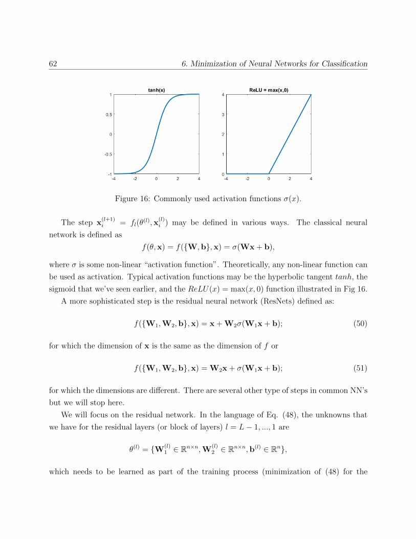
62 6. Minimization of Neural Networks for Classification
Figure 16: Commonly used activation functions σ(x).
The step x(l+1)i = fl(θ
(l),x(l)i ) may be defined in various ways. The classical neural
network is defined as
f(θ,x) = f(W,b,x) = σ(Wx + b),
where σ is some non-linear “activation function”. Theoretically, any non-linear function can
be used as activation. Typical activation functions may be the hyperbolic tangent tanh, the
sigmoid that we’ve seen earlier, and the ReLU(x) = max(x, 0) function illustrated in Fig 16.
A more sophisticated step is the residual neural network (ResNets) defined as:
f(W1,W2,b,x) = x + W2σ(W1x + b); (50)
for which the dimension of x is the same as the dimension of f or
f(W1,W2,b,x) = W2x + σ(W1x + b); (51)
for which the dimensions are different. There are several other type of steps in common NN’s
but we will stop here.
We will focus on the residual network. In the language of Eq. (48), the unknowns that
we have for the residual layers (or block of layers) l = L− 1, ..., 1 are
θ(l) = W(l)1 ∈ Rn×n,W
(l)2 ∈ Rn×n,b(l) ∈ Rn,
which needs to be learned as part of the training process (minimization of (48) for the
63 6. Minimization of Neural Networks for Classification
training set).
Remark: the definition of layer Some people define each operation in the function
above as “layer” (for example, the addition of bias, the multiplication of W, the non-linear
function σ etc, each one is a different “layer”). The whole residual network step is then
defined as a block of layers.
6.4 Computing the gradient of NN’s: back-propagation
The constrained objective (48) can be minimized in various ways. The most common way to
solve it is by SGD. To apply SGD, we need to be able to compute the gradient, and somehow
handle the constraint. From practical reasons, the constraint is handled by elimination,
removing x(l) as unknowns. We get a nested chain of functions of the type
F (θ(i)3i=1) = f3(x(3), θ(3)) = f3(f2(x(2), θ(2)), θ(3)) = f3(f2(f1(x(1), θ(1)), θ(2)), θ(3)), (52)
where in this example, L = 3, and x(1) is the given data.
Let’s assume that all the quantities above are scalars, i.e., fi(x, θ) : (R,R) → R so each
derivative will also be a scalar. We wish to get the derivative of f3 in (52) with respect to
θ(1), θ(2), θ(3). We get a special structure using inner derivatives:
∂F
∂θ(3)=
∂f3
∂θ(53)
∂F
∂θ(2)=
∂f3
∂x· ∂f2
∂θ(54)
∂F
∂θ(1)=
∂f3
∂x· ∂f2
∂x· ∂f1
∂θ. (55)
The order of multiplications in (53) could have been different as these are all scalars, but it
turns out (as we will see later) that the right way to put it is
∂F
∂θ(3)=
∂f3
∂θ(56)
∂F
∂θ(2)=
∂f2
∂θ· ∂f3
∂x(57)
∂F
∂θ(1)=
∂f1
∂θ· ∂f2
∂x· ∂f3
∂x. (58)
64 6. Minimization of Neural Networks for Classification
This is the right order if all functions where vector functions of vector unknowns. To compute
(52) we start from f1, and end at f3. That is a forward pass. To compute the gradient
of F , we start from f3 and propagate backwards all the way to f1. That is called the
backpropagation pass.
To illustrate the right order we will rewrite (52) in vector form for L = 2, but also include
the scalar loss function at the end. We denote: ` = `(x,θ), and fi = fi(x,θ). That is, each
function fi is defined for two unknowns and is not “aware” of its location in the network.
F (θ(i)3i=1) = `(f2(x(2),θ(2)),θ(3)) = `(f2(f1(x(1),θ(1)),θ(2)),θ(3)). (59)
We wish to compute the gradient of F with respect to all the parameters (in order to use an
optimization algorithm):
∇F =
∇θ(3)F
∇θ(2)F
∇θ(1)F
Since θ(3) only involves with `, then the gradient with respect to θ(3) is simply:
∇θ(3)F = ∇θ`.
The rest of the gradient requires the chain rule, because it involves with fi inside `. We know
that simple Taylor series is given by
`(x + δx,θ) ≈ `(x,θ) + δxT∇x`.
Also, for every x and θ
f2(x + δx,θ) ≈ f2(x,θ) +∂f2
∂xδx.
Now, assume that instead of x + δx, we put f1(x(1),θ(1) + δθ(1)) = f1(x(1),θ(1)) + δf1. We get
f2(f1(x(1),θ(1) + δθ(1)),θ(2)) ≈ f2(f1(x(1),θ(1)),θ(2)) +∂f2
∂xδf1
≈ f2(f1(x(1),θ(1)),θ(2)) +∂f2
∂x
∂f1
∂θδθ(1).
65 6. Minimization of Neural Networks for Classification
So, overall δf2 = ∂f2∂x
∂f1∂θδθ(1). Now we plug:
`(f2 + δf2,θ(3)) ≈ `(f2,θ
(3)) + δfT2 ∇x`
= `(f2,θ(3)) +
(∂f2
∂x
∂f1
∂θδθ(1)
)T∇x`
= `(f2,θ(3)) +
(δθ(1)
)> ∂f1
∂θ
T ∂f2
∂x
T
∇x`
From here, the gradient of (59) is
∇θ(2)F =∂f2
∂θ
T
∇x`
∇θ(1)F =∂f1
∂θ
T ∂f2
∂x
T
∇x`
To sum up, for each layer f(x,θ), we need to compute the Jacobian (with respect to each
of the parameters) transpose multiplied with some vector. We will define this operation for
our residual network.
6.5 Computing derivatives of Neural Networks
6.5.1 The derivatives of matrix-vector and matrix-matrix multiplications
We will start with a rather simple auxiliary computation that will help us later. Assume
y = Wx; W ∈ Rt×n; y ∈ Rt; x ∈ Rn
We’ve already seen earlier in the course that ∂y∂x
= W, and hence simply ∂y∂x
T= WT .
Now we’ll examine the case of the derivative with respect to W:
y + δy = (W + δW)x⇒ δy = δWx.
Using different writing, we wish to have
δWx ≡ ∂y
∂Wvec(δW),
66 6. Minimization of Neural Networks for Classification
where ∂y∂W∈ Rt×tn is a Jacobian matrix and the operation vec(W) is the concatanation of the
columns of W one after the other into a long vector of size tn (also known as column-stack
representation, achieved by the operator [:] in Julia). We need to know how to define ∂y∂W
and to compute its transpose times a vector.
To obtain this, we will start with a few definitions to let us work with matrices and their
derivatives. To deal with matrices as unknowns, we will transfer them into vectors first,
compute the derivative and transfer them back.
In particular we will use the following identities:
(A⊗B)T = AT ⊗BT (60)
AXB = C ⇒ (BT ⊗ A)vec(X) = vec(C) (61)
Back to our auxiliary computation:
∂y
∂Wvec(δW) = δWx,
then by (61) we have
IδWx = (xT ⊗ I)vec(δW)⇒ ∂y
∂W= xT ⊗ I. (62)
By the identity in (60) we have that the Jacobian trasposed times some vector is given by:
(xT ⊗ I)Tv = (x⊗ I)v =after de-column-stacking vxT ∈ Rt×n (63)
where v is some vector of the same size of y. vxT is the same size of W without column
stack. Like in the case of Logistic Regression, if we have many data samples xi stacked in a
matrix column-wise:
X = [x1|x2|x3|...|xm],
67 6. Minimization of Neural Networks for Classification
and we wish to take the derivative of Y = WX with respect to W. Similarly to before, the
Jacobian transposed times a matrix V of the same size as Y is given by:
(X⊗ I)V =after de-column-stacking
∑i
vix>i = VX>.
this has to be verified.
6.5.2 The derivatives of standard neural networks
Let’s look at our network step:
y = f(θ,x) = σ(Wx + b).
In our backpropagation, we should multiply different vectors v of size similar to y with the
transpose of the Jacobian with respect to each of the weights and unknowns x ∈ Rn,W ∈Rk×n,b ∈ Rk.
The derivative with respect to b ∈ Rk:
y + δy = σ(Wx + b + δb)
≈ y + diag(σ′(Wx + b))δb
⇒ ∂y
∂b= diag(σ′(Wx + b)) ∈ Rk×k.
The derivative with respect to W ∈ Rk×n:
y + δy = σ((W + δW)x + b)
≈ diag(σ′(Wx + b))δWx
⇒ ∂y
∂W= diag(σ′(Wx + b))(xT ⊗ I) ∈ Rk×kn.
In the last equation we used (62), and to multiply the transpose of this matrix with a vector
v, we need to follow (63).
68 6. Minimization of Neural Networks for Classification
The derivative with respect to x:
y + δy = σ(W(x + δx) + b)
≈ y + diag(σ′(Wx + b))Wδx
⇒ ∂y
∂x= diag(σ′(Wx + b))W ∈ Rk×n.
6.5.3 The derivatives of residual networks
Let’s look again at our residual network step:
y = f(θ,x) = x + W2σ(W1x + b).
In our backpropagation, we should multiply different vectors v of size similar to f(θ,x) with
the transpose of the Jacobian with respect to each of the weights and unknowns x,W2,W1,b.
The derivative with respect to b:
y + δy = x + W2σ(W1x + b + δb)
≈ y + W2diag(σ′(W1x + b))δb
⇒ ∂y
∂b= W2diag(σ′(W1x + b)) ∈ Rn×n.
The derivative with respect to W1:
y + δy = x + W2σ((W1 + δW1)x + b)
≈ y + W2diag(σ′(W1x + b))δW1x
⇒ ∂y
∂W1
= W2diag(σ′(W1x + b))(xT ⊗ I) ∈ Rn×n2
.
In the last equation we used (62), and to multiply the transpose of this matrix with a vector
v, we need to follow (63).
69 6. Minimization of Neural Networks for Classification
The derivative with respect to W2:
y + δy = x + (W2 + δW2)σ(W1x + b)
= y + δW2σ(W1x + b)
⇒ ∂y
∂W2
= (σ(W1x + b)T ⊗ I) ∈ Rn×n2
.
Here, again, we used (62), only with respect to σ(W1x + b) instead of x. To multiply the
transpose of this matrix with a vector v, we need to follow (63).
The derivative with respect to x:
y + δy = x + δx + W2σ(W1(x + δx) + b)
≈ y + δx + W2diag(σ′(W1x + b))W1δx
⇒ ∂y
∂x= I + W2diag(σ′(W1x + b))W1 ∈ Rn×n.
6.6 Gradient and Jacobian verification
Each time we compute a non-linear function and its derivative, we need to make sure that
our derivations are correct. It is better not to test this though the whole optimization process
of our system, and do it part by part. This way, (1) we will be able to identify the errors in
the right places, and (2) we won’t be confused in the case where our optimization algorithm
really does not supposed to work (the lack of minimization is a “feature instead of a bug”).
The gradient test: The simplest case is achieved for the gradient of a scalar function.
Let d be a random vector, such that ‖d‖ = O(1). Then, we know that
f(x + εd) = f(x) + εdT∇f +O(ε2)
Suppose that we have a code grad(x) for computing ∇f(x). Then, we can compare
|f(x + εd)− f(x)| = O(ε) (64)
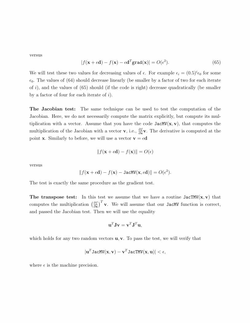
versus
|f(x + εd)− f(x)− εdTgrad(x)| = O(ε2). (65)
We will test these two values for decreasing values of ε. For example εi = (0.5)iε0 for some
ε0. The values of (64) should decrease linearly (be smaller by a factor of two for each iterate
of i), and the values of (65) should (if the code is right) decrease quadratically (be smaller
by a factor of four for each iterate of i).
The Jacobian test: The same technique can be used to test the computation of the
Jacobian. Here, we do not necessarily compute the matrix explicitly, but compute its mul-
tiplication with a vector. Assume that you have the code JacMV(x,v), that computes the
multiplication of the Jacobian with a vector v, i.e., ∂f∂x
v. The derivative is computed at the
point x. Similarly to before, we will use a vector v = εd
‖f(x + εd)− f(x)‖ = O(ε)
versus
‖f(x + εd)− f(x)− JacMV(x, εd)‖ = O(ε2).
The test is exactly the same procedure as the gradient test.
The transpose test: In this test we assume that we have a routine JacTMV(x,v) that
computes the multiplication(∂f∂x
)Tv. We will assume that our JacMV function is correct,
and passed the Jacobian test. Then we will use the equality
uTJv = vTJTu,
which holds for any two random vectors u,v. To pass the test, we will verify that
|uTJacMV(x,v)− vTJacTMV(x,u)| < ε,
where ε is the machine precision.


![Numerical Differentiation & Integration [0.125in]3.375in0 ...mamu/courses/231/Slides/CH04_4A.pdf · Numerical Differentiation & Integration Composite Numerical Integration I Numerical](https://img.pdfslide.net/doc/110x75/5b1fb63d7f8b9a112c8b4a5d/numerical-differentiation-integration-0125in3375in0-mamucourses231slidesch044apdf.jpg)


![MKG - By Treister [ENG] - Oral Chronic GVHD - PPT](https://img.pdfslide.net/doc/110x75/5695cf301a28ab9b028cfad1/mkg-by-treister-eng-oral-chronic-gvhd-ppt.jpg)