Numerical Prediction of Mesoscale Weather for... · 2013-02-17 · Numerical Prediction of Mesoscale Weather 7th APEC - Tsukuba International Conference , 17 March 2013, Bunkyo School,

Numerical Prediction of Mesoscale Weather

7th APEC - Tsukuba International Conference , 17 March 2013, Bunkyo School, Tsukuba University

Kazuo Saito [email protected]

1. History of numerical weather prediction

2. Fundamental equations for atmosphere

3. Importance of the initial condition

4. Ensemble prediction

5. The K-computer project

Meteorological Research Institute (MRI)

1. History of Numerical Weather Prediction

Numerical Weather Prediction (NWP)

.. predicts future state of the atmosphere quantitatively by time-integrating

laws of physics

.. regarded as one of the best application fields of computational physics from

the earliest period

Bjerknes (1904) pointed out possibility of weather prediction based on

dynamics and physics

Richardson (1922) tried weather prediction by solving the equations of fluid

with hand calculation but failed by overwhelming of noises

o(10hPa)

145hPa/6hour

computation

time

surface pressure

Horizontal and vertical grid taken by Richardson (1922)

Dawn of numerical weather prediction

1946 Pennsylvania Univ. Developed the

first digital computer (ENIAC)

23 word memories, 18,800 tubes

(300FLOPS)

Von Neumann of Institute for Advanced

Study, Princeton Univ. proposed application

to weather prediction

1950 First success of 24 hour forecast using

ENIAC by Charney et al.

Grid distance 736 km at 45N

Number of grid points 15×18

One level (500hPa)

2-dimensional barotropic model which predicts

the absolute vorticity preservation law

d/dt(f +ζ) = 0

35 days for two 24 hour computations

NWP in Japan

1959 Japan Meteorological Agency implemented IBM704

core Memory of 8 K words (36 bit)

1960 Operation started with a northern hemispheric barotropic model

(381 km, one level)

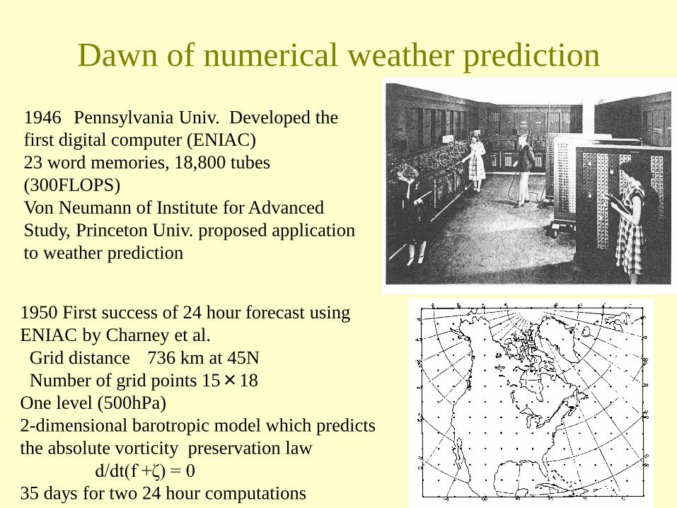
NWP models at JMA (1988-)

Operation of

JMA-NHM

(10km) (5km) (2km)

2. Fundamental equations for atmosphere

Diagnostic equation

Prognostic equations

• Momentum equation（three wind components: u, v and w ）

• Continuity equation（pressure: p）

• Thermodynamic equation (temperature: T)

Six variables which describe the state of dry atmosphere:

three velocity components, pressure, temperature and density

In the case of moist atmosphere, preservation of water substances and

the phase change must be considered (cloud micro-physics).

• State equation (density: r)

Momentum equation

wdifgz

p

td

dw

vdify

p

td

dv

udifx

p

td

du

.1

.1

.1

r

r

r

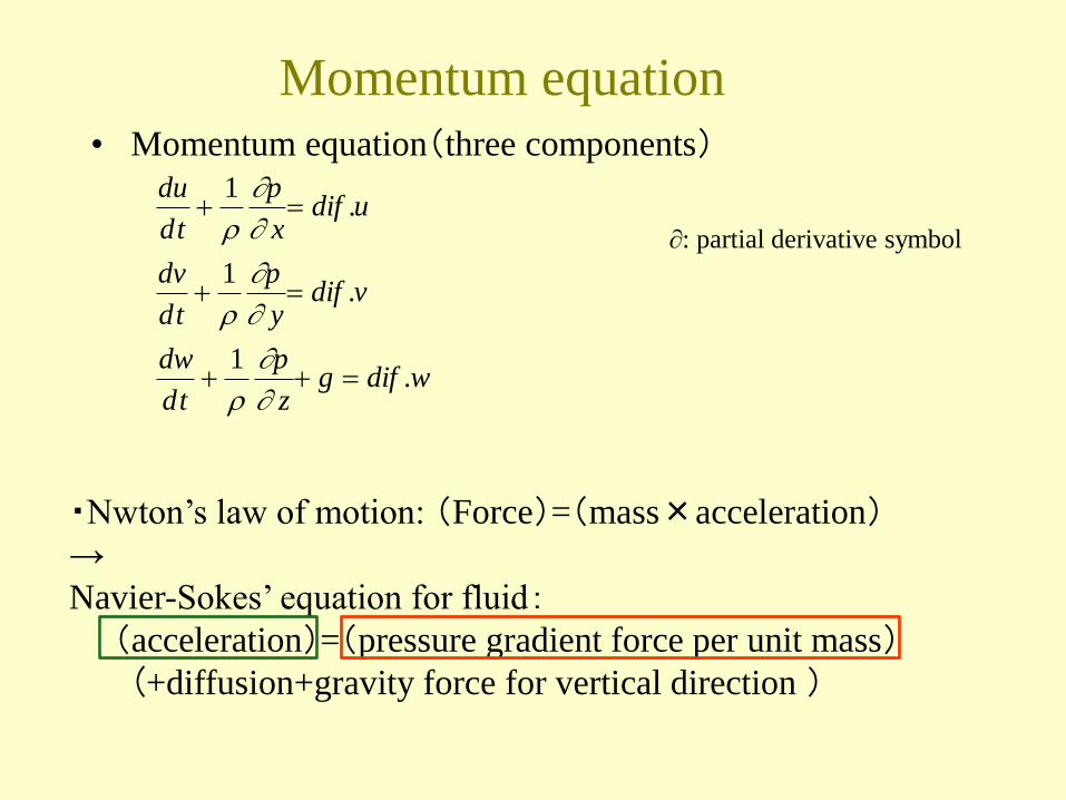
• Momentum equation（three components）

・Nwton’s law of motion: （Force）=（mass×acceleration）

→

Navier-Sokes’ equation for fluid：

（acceleration）=（pressure gradient force per unit mass）

(+diffusion+gravity force for vertical direction ）

∂: partial derivative symbol

Momentum equation

wdifgz

p

td

dw

vdify

p

td

dv

udifx

p

td

du

.1

.1

.1

r

r

r

• Momentum equation（three components）

・Nwton’s law of motion: （Force）=（mass×acceleration）

→

Navier-Sokes’ equation for fluid：

（acceleration）=（pressure gradient force per unit mass）

(+diffusion+gravity acceleration for vertical direction ）

∂: partial derivative symbol

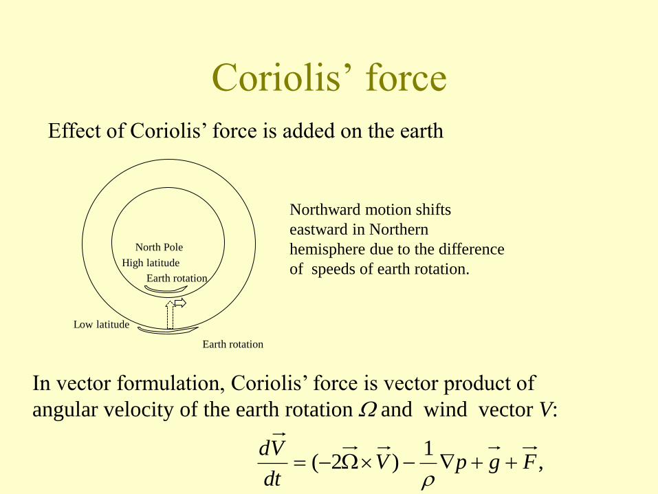
Coriolis’ force

Effect of Coriolis’ force is added on the earth

,1

)2( FgpVdt

Vd

r

Earth rotation

Earth rotation

North Pole

Low latitude

High latitude

In vector formulation, Coriolis’ force is vector product of

angular velocity of the earth rotation and wind vector V:

Northward motion shifts

eastward in Northern

hemisphere due to the difference

of speeds of earth rotation.

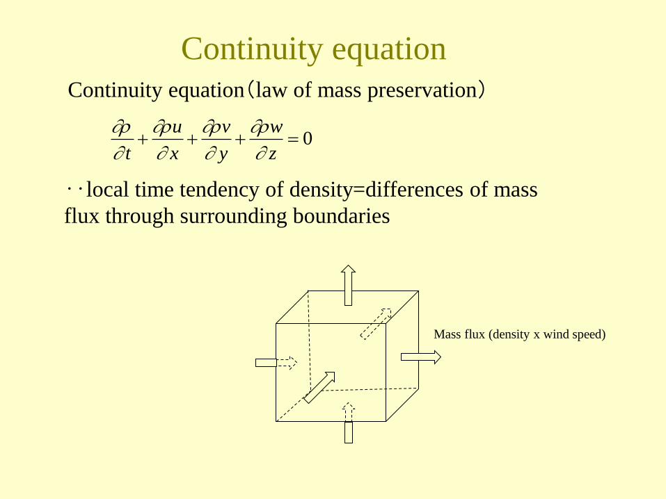
Continuity equation（law of mass preservation）

0z

w

y

v

x

u

t

r

r

r

r

‥local time tendency of density=differences of mass

flux through surrounding boundaries

Continuity equation

Mass flux (density x wind speed)

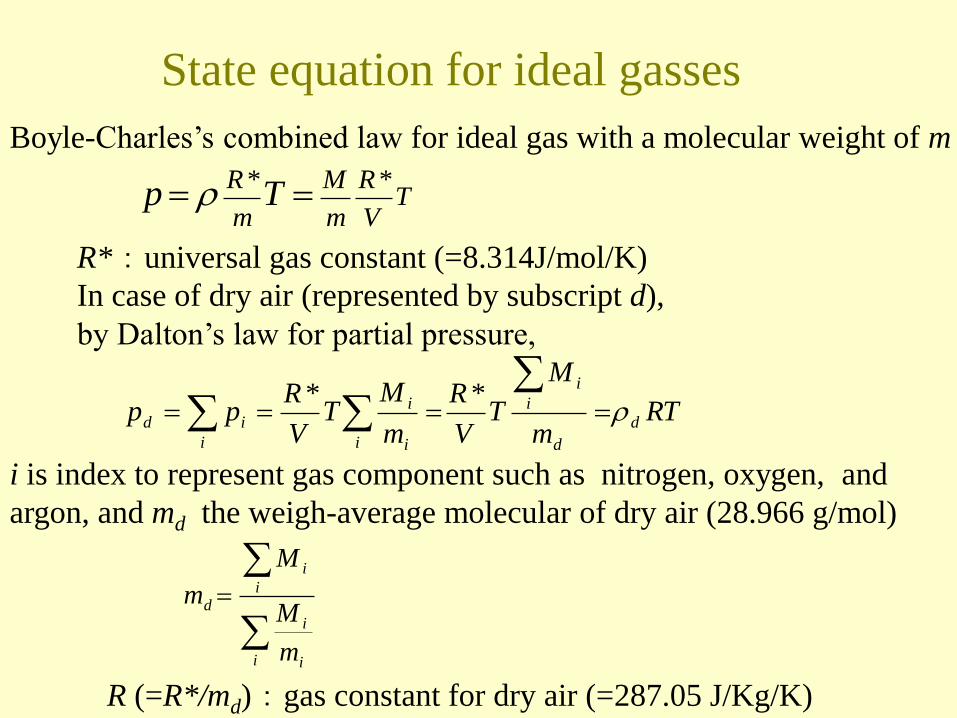
State equation for ideal gasses

i is index to represent gas component such as nitrogen, oxygen, and

argon, and md the weigh-average molecular of dry air (28.966 g/mol)

Boyle-Charles’s combined law for ideal gas with a molecular weight of m

R*：universal gas constant (=8.314J/mol/K)

In case of dry air (represented by subscript d),

by Dalton’s law for partial pressure,

R (=R*/md)：gas constant for dry air (=287.05 J/Kg/K)

TV

R

m

M

m

RTp

** r

RTm

M

TV

R

m

MT

V

Rpp d

d

i

i

i i

i

i

id r

**

i i

i

i

i

d

m

M

M

m

Forces on air and acceleration

contour of pressure

Low pressure

Pressure gradient force

Coriolis’ force

Frictional force Pressure gradient force

Gravity force

Isobaric plain

high pressure

low pressure

Veridical pressure gradient

force usually balances with

the gravity force

(hydrostatic equilibrium)

wind direction

Sum of pressure gradient

force, Coriolis’ force and

frictional force accelerates

the air mass toward the low

pressure

acceleration

acceleration

hydrostatic equilibrium 01

gzd

dp

r

→ RT

g

zd

dp

p

1→

mRT

gz

epp

0→

RT

gp

zd

d)(log

… well-known barometric height formula

(pressure-height equation)

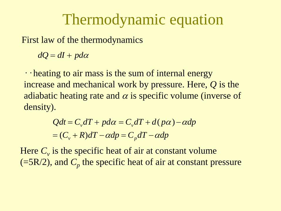
Thermodynamic equation

pddIdQ

First law of the thermodynamics

‥heating to air mass is the sum of internal energy

increase and mechanical work by pressure. Here, Q is the

adiabatic heating rate and is specific volume (inverse of

density).

dpdTCdpdTRC

dppddTCpddTCQdt

pv

vv

)(

)(

Here Cv is the specific heat of air at constant volume

(=5R/2), and Cp the specific heat of air at constant pressure

Finite discretization In the numerical model, differential equation is discretized by finite

difference, based on the Taylor series expansion:

Here, f ’ (f’’) is the first (second) derivative of the function f.

The second order centered difference can be obtained as :

..)(''2

)()(')()(

..)(''2

)()(')()(

2

2

xfx

xxfxfxxf

xfx

xxfxfxxf

2)(2

)()(xO

x

xxfxxf

x

f

or, in staggered grid,

2)2

(

)2

()2

(x

Ox

xxf

xxf

x

f

For advection term in momentum equations, higher order schemes are used e.g.,

4)2

(3

)2

3()

2

3(

8

1)

2()

2(

8

9 xO

x

xxf

xxf

x

xxf

xxf

x

f

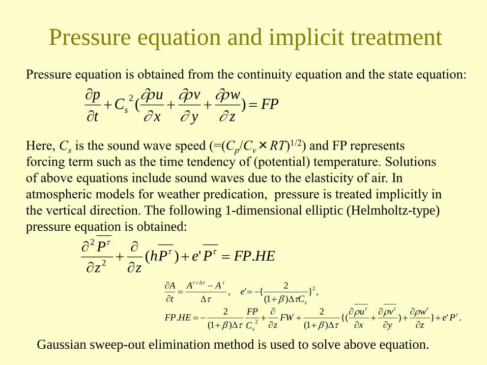
Pressure equation and implicit treatment

Here, Cs is the sound wave speed (=(Cp/Cv×RT)1/2) and FP represents

forcing term such as the time tendency of (potential) temperature. Solutions

of above equations include sound waves due to the elasticity of air. In

atmospheric models for weather predication, pressure is treated implicitly in

the vertical direction. The following 1-dimensional elliptic (Helmholtz-type)

pressure equation is obtained:

HEFPPePhzz

P.')(

2

2

.'}){()1(

2

)1(

2.

,})1(

2{',

2

2

rrr

Pez

w

y

v

x

uFW

zC

FPHEFP

Ce

AA

t

A

s

s

Gaussian sweep-out elimination method is used to solve above equation.

Pressure equation is obtained from the continuity equation and the state equation:

FPz

w

y

v

x

uC

t

ps

)(

2

r

r

r

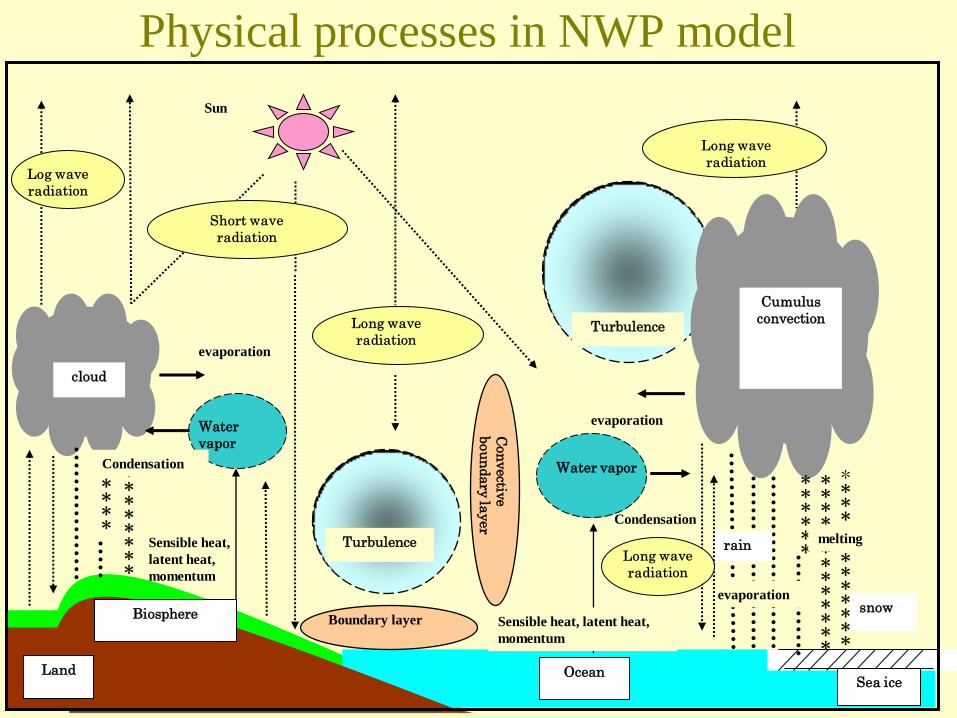
Condensation

Cumulus

convection

Ocean Sea ice

rain

＊＊＊＊＊＊＊＊＊＊＊＊＊

＊＊＊＊＊＊＊＊＊＊＊＊＊

snow

＊＊＊＊＊＊

cloud

＊＊＊＊＊＊＊＊＊

＊＊＊＊＊

Water

vapor

Water vapor C

on

vectiv

e

bou

nd

ary

layer

Sensible heat, latent heat,

momentum

Sun

Boundary layer

Land

Biosphere

evaporation

melting

evaporation

evaporation

Condensation

Turbulence

Turbulence Sensible heat,

latent heat,

momentum

Physical processes in NWP model

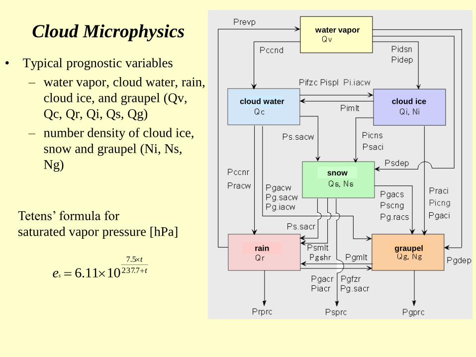
Cloud Microphysics

• Typical prognostic variables

– water vapor, cloud water, rain,

cloud ice, and graupel (Qv,

Qc, Qr, Qi, Qs, Qg)

– number density of cloud ice,

snow and graupel (Ni, Ns,

Ng)

graupel rain

snow

cloud ice cloud water

water vapor

Tetens’ formula for

saturated vapor pressure [hPa]

t

t

se

7.237

5.7

1011.6

In bulk method, the size distribution function of water substance is

expressed by the inverse exponential function of the particle diameter D.

Bulk cloud microphysics

DeNDN 0)(

Fall-out terminal velocity of

particle is given as a power

function of D by the

Stokes’ law in the form of

baDDV )(

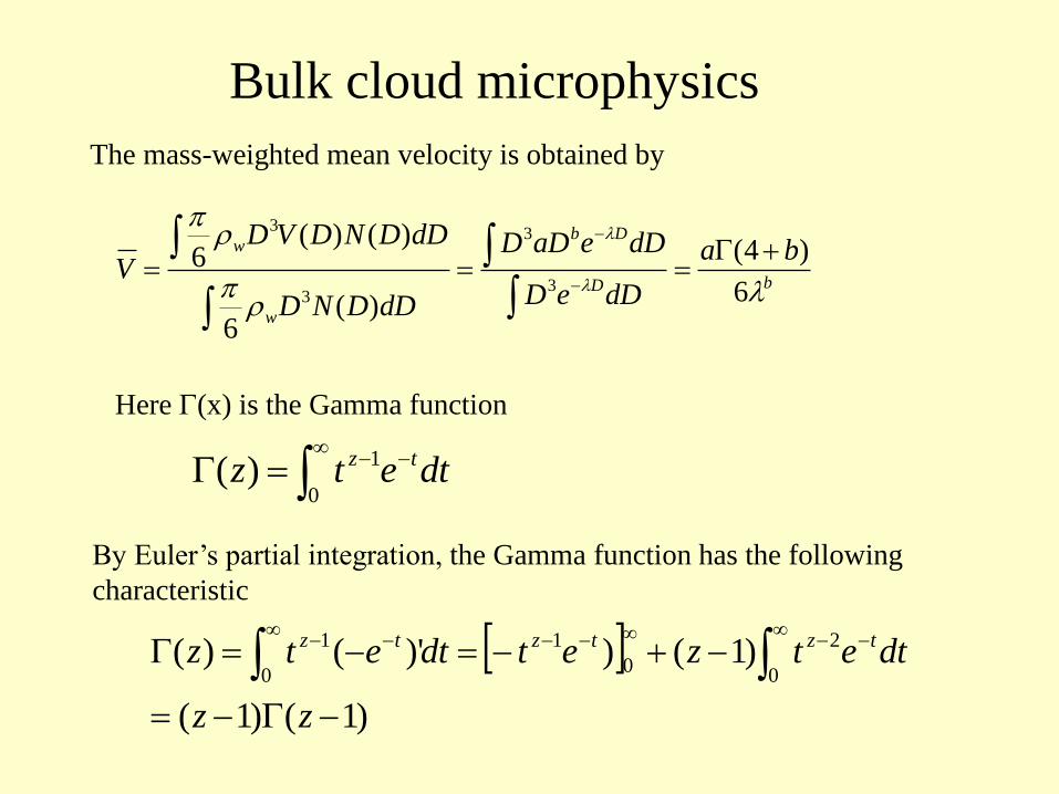
Bulk cloud microphysics

The mass-weighted mean velocity is obtained by

Here G(x) is the Gamma function

bD

Db

w

w ba

dDeD

dDeaDD

dDDND

dDDNDVD

Vr

r

6

)4(

)(6

)()(6

3

3

3

3

G

)1()1(

)1())'()(0

2

0

1

0

1

G

G

zz

dtetzetdtetz tztztz

By Euler’s partial integration, the Gamma function has the following

characteristic

dtetz tz

G0

1)(

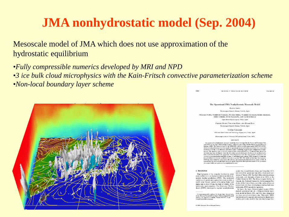
•Fully compressible numerics developed by MRI and NPD

•3 ice bulk cloud microphysics with the Kain-Fritsch convective parameterization scheme

•Non-local boundary layer scheme

Mesoscale model of JMA which does not use approximation of the

hydrostatic equilibrium

JMA nonhydrostatic model (Sep. 2004)

Polar low simulation with JMA NHM

Horizontal resolution 2km

Initial time 15UTC 21 January 1997

Cloud resolving model

GMS satellite IR image Cloud resolving simulation of a polar

low (Yanase et al., 2002; GRL)

Left) GMS satellite visible-Image at 15JST 14 January 2001

Right) Total water simulated by NHM with a horizontal resolution of 1 km

Eito et al. (2010; JMSJ)

Cloud resoling simulation of winter monsoon clouds

over the Sea of Japan using Earth Simulator

3. Importance of the initial condition

Major difference between climate projection and NWP

・the same point

predict future state of the atmosphere quantitatively by time-integrating laws of

physics.

・major difference

Climate projection

‥projects climate response to change of global environment such as CO2, SST

⇒boundary condition and radiation-convection equilibrium are important

NWP

‥predicts weather of a specific day in short time range

⇒initial condition and time evolution are important

xyx

yxyxx

dpp

ppp

oobb

oobbob

)()(

)()(),|(

Baysian estimation

)]()([maxˆoobb pp yxx

x

xb xa yo x

PDF of observation PDF of first

guess

ｘ： analysis variable ｘｂ： first guess of ｘｙｏ： observation data ｐ（・｜・）： conditional probabilistic density function (PDF)

Bayesian theorem

（if ｘｂ and ｙｏ are independent,

Maximum likelihood estimation in

data assimilation

}2

)(exp{

2

1)(

}2

)(exp{

2

1)(

2

2

2

2

2

2

o

o

o

oo

b

b

b

bb

yyyp

xxp

x

}2

)(exp{

2

1

)()(

)()(),|(

2

2

2a

a

a

oobb

oobbob

xx

dpp

ppp

xyx

yxyxx

The conditional PDF of x with background xb and observation yo is normal as

Where analysis xa and its standard deviation σa are

222

222

111

oba

o

o

b

b

a

a yxx

xb xa yo x

PDF of observation PDF of first

guess

Maximum likelihood

estimation

If PDFs of the first guess and observation are Gaussian normal

distribution as

)(22

22

oa

oaboa

yxx

→

Analysis is weighted mean of first guess and observation, and analysis error

becomes smaller than the errors of first guess and observation.

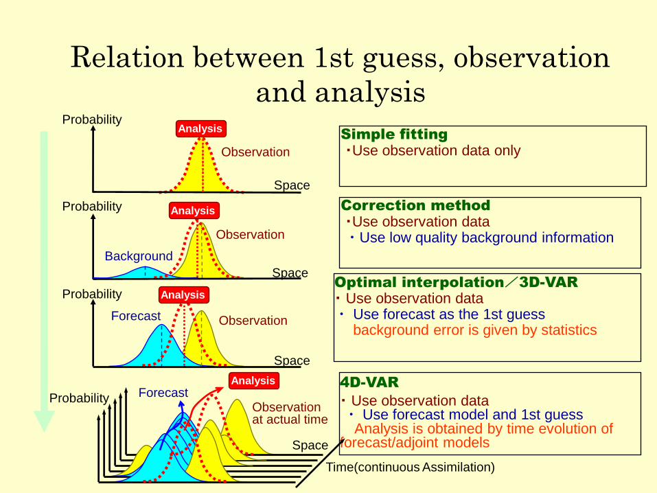
Observation

Simple fitting ・Use observation data only

Correction method ・Use observation data ・Use low quality background information

Probability

Probability

Observation

Background

Analysis

Analysis

Optimal interpolation／3D-VAR

・ Use observation data ・ Use forecast as the 1st guess background error is given by statistics

4D-VAR

・ Use observation data ・ Use forecast model and 1st guess Analysis is obtained by time evolution of forecast/adjoint models

Space

Probability

Observation Forecast

Space

Probability Observation at actual time

Forecast

Time(continuous Assimilation)

Analysis

Analysis

Space

Space

Relation between 1st guess, observation

and analysis

4Dimensional –Variational method

x

Cost

function :

First guess

Forecast

from

analysis observation

Jo

Jo

Jo

Jo

Jb

xb

21UTC 00UTC

Assimilation window

time

c

oobb

cob

JyHMxyHMxxxxx

JJJJ

0

1T

000

1T

00 R2

1B

2

1

cxob

cxoxbxx

JyHMxxx

JJJJ

00

1TT00

1

0000

RHMB

Gradient of

cost

function:

First guess

observation

observation

Observation

x0

Adjoint model

Forecast model

Penalty term

Observation data can be assimilated at observation time

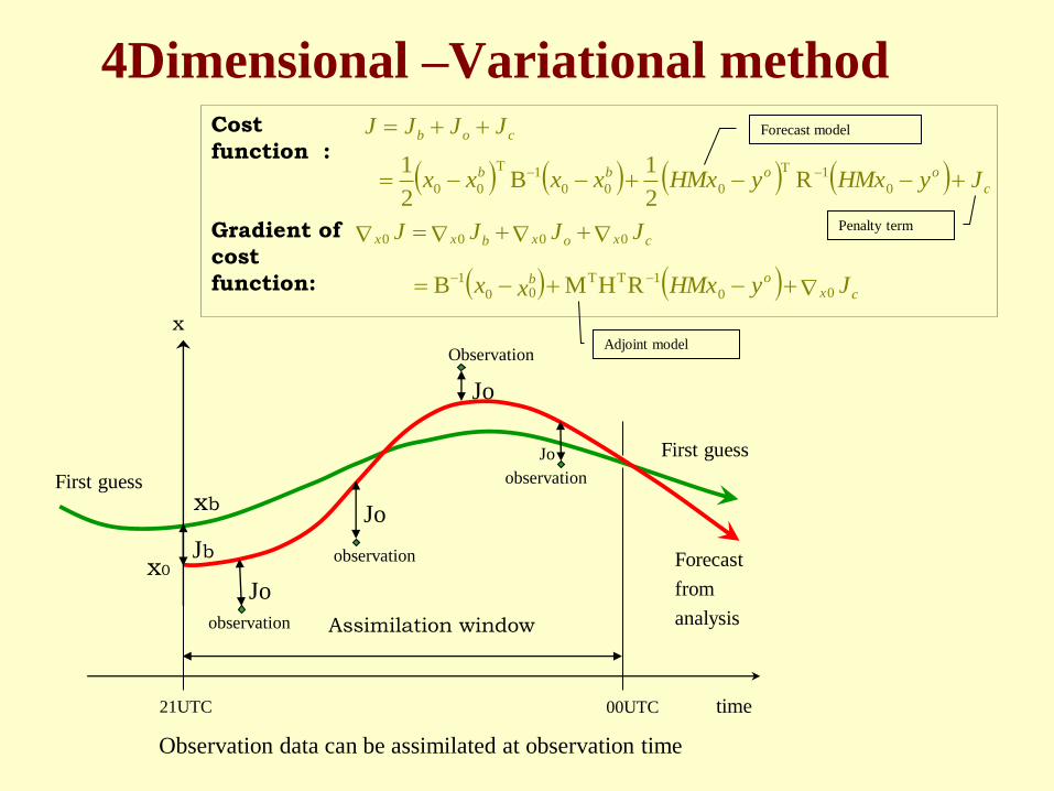
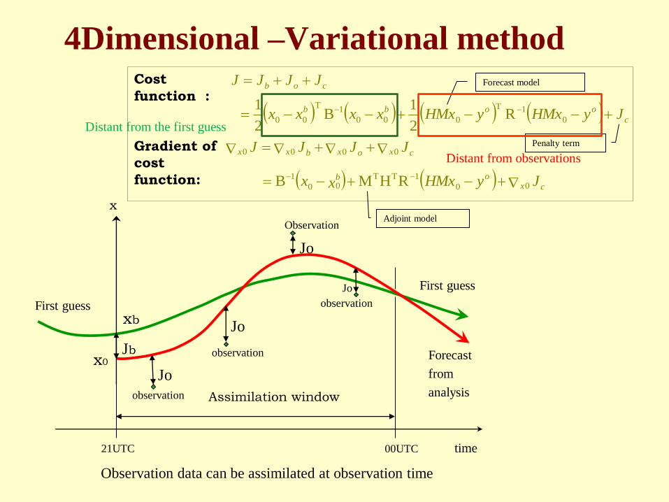
4Dimensional –Variational method

x

Cost

function :

First guess

Forecast

from

analysis observation

Jo

Jo

Jo

Jo

Jb

xb

21UTC 00UTC

Assimilation window

time

c

oobb

cob

JyHMxyHMxxxxx

JJJJ

0

1T

000

1T

00 R2

1B

2

1

cxob

cxoxbxx

JyHMxxx

JJJJ

00

1TT00

1

0000

RHMB

Gradient of

cost

function:

First guess

observation

observation

Observation

x0

Adjoint model

Forecast model

Penalty term

Observation data can be assimilated at observation time

Distant from the first guess

Distant from observations

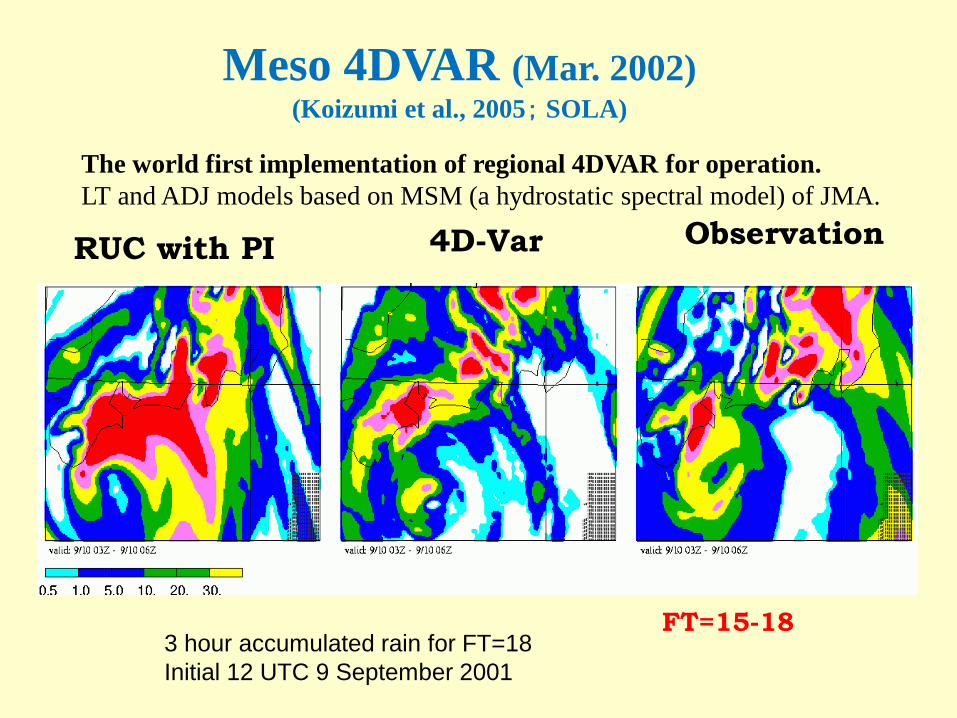
RUC with PI 4D-Var Observation

FT=15-18 3 hour accumulated rain for FT=18

Initial 12 UTC 9 September 2001

Meso 4DVAR (Mar. 2002) (Koizumi et al., 2005； SOLA)

The world first implementation of regional 4DVAR for operation.

LT and ADJ models based on MSM (a hydrostatic spectral model) of JMA.

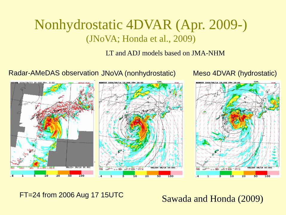
Radar-AMeDAS observation JNoVA (nonhydrostatic) Meso 4DVAR (hydrostatic)

FT=24 from 2006 Aug 17 15UTC

Nonhydrostatic 4DVAR (Apr. 2009-) (JNoVA; Honda et al., 2009)

Sawada and Honda (2009)

LT and ADJ models based on JMA-NHM

Threat score of MSM Mar.2001-Nov.2011 (FT=0-15)

Nonhydrostatic

model

Meso4DVAR

10km to 5km

Nonhydrostatic

4DVAR

GPS TPWV

Radar

Reflectivity

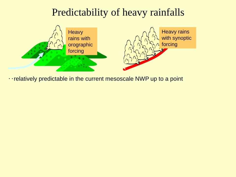
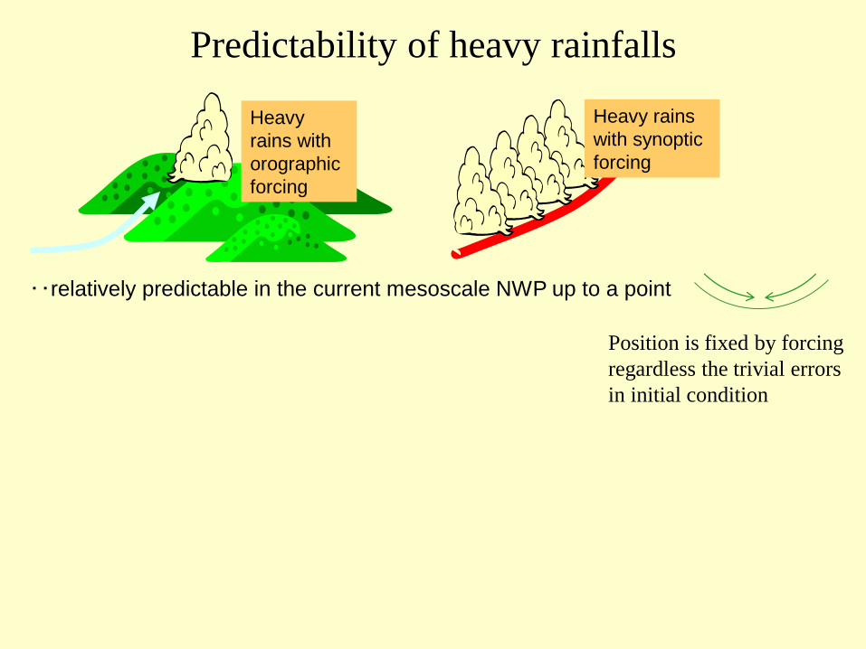
Heavy rains

with synoptic

forcing

Heavy

rains with

orographic

forcing

‥relatively predictable in the current mesoscale NWP up to a point

Predictability of heavy rainfalls

Heavy rains

with synoptic

forcing

Heavy

rains with

orographic

forcing



Position is fixed by forcing

regardless the trivial errors

in initial condition

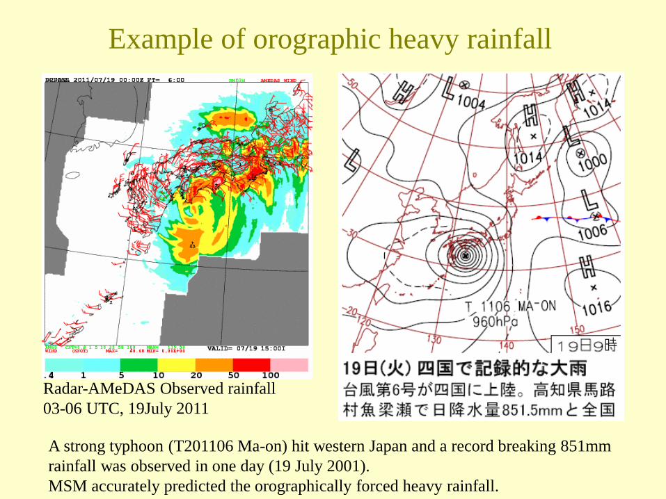
Example of orographic heavy rainfall

Radar-AMeDAS Observed rainfall

03-06 UTC, 19July 2011

MSM prediction FT=21

03-06 UTC, 19July 2011

A strong typhoon (T201106 Ma-on) hit western Japan and a record breaking 851mm

rainfall was observed in one day (19 July 2001).

MSM accurately predicted the orographically forced heavy rainfall.

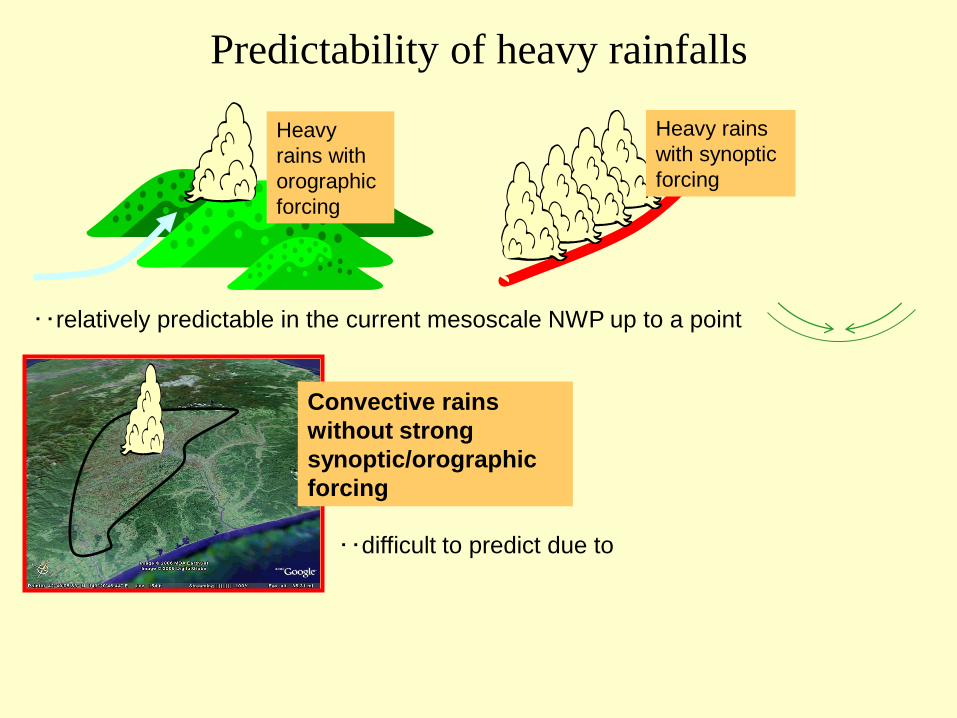
Heavy rains

with synoptic

forcing

Heavy

rains with

orographic

forcing


Convective rains

without strong

synoptic/orographic

forcing


‥difficult to predict due to

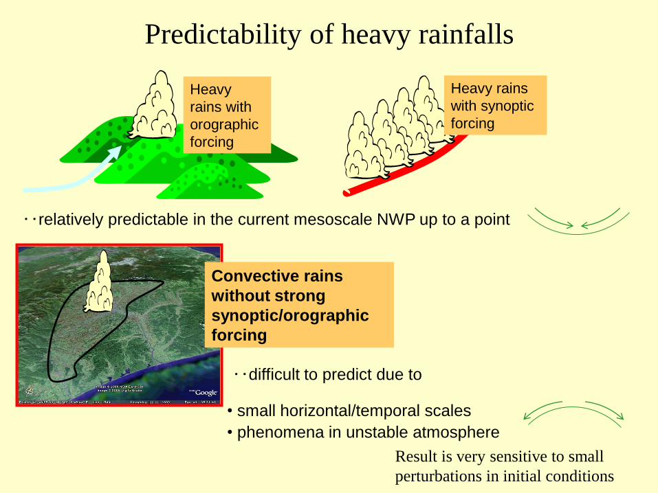
Heavy rains

with synoptic

forcing

Heavy

rains with

orographic

forcing


Convective rains

without strong

synoptic/orographic

forcing


• small horizontal/temporal scales

• phenomena in unstable atmosphere

‥difficult to predict due to

Result is very sensitive to small

perturbations in initial conditions

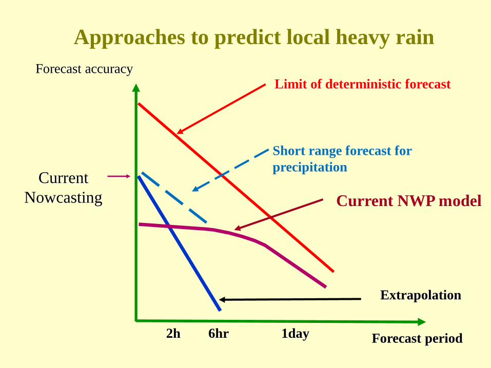
Forecast period

Forecast accuracy

2h 6hr 1day

Extrapolation

Limit of deterministic forecast

Current

Nowcasting

Short range forecast for

precipitation

Current NWP model

Approaches to predict local heavy rain

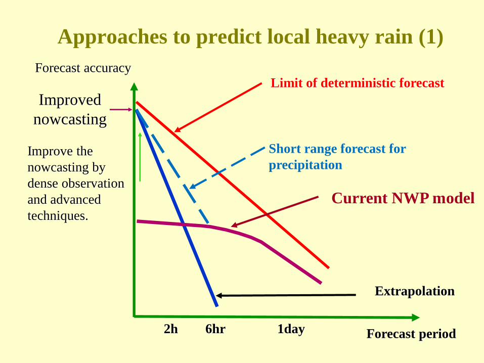
Approaches to predict local heavy rain (1)

Forecast period

Forecast accuracy

2h 6hr 1day

Extrapolation


Improved

nowcasting


precipitation

Current NWP model

Improve the

nowcasting by

dense observation

and advanced

techniques.

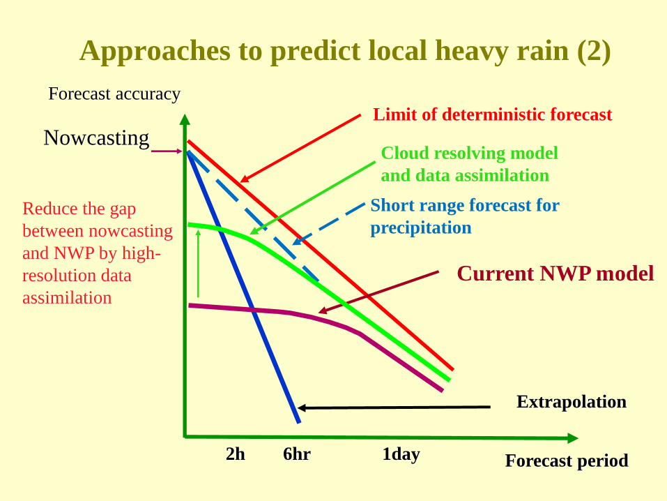
Forecast period

Forecast accuracy

2h 6hr 1day

Extrapolation


Nowcasting


precipitation


and data assimilation

Reduce the gap

between nowcasting

and NWP by high-

resolution data

assimilation

Current NWP model


Local Heavy rainfall on September 2005 in Tokyo

Local heavy rainfall on 4 September 2005

100mm precipitation in 1 hour was observed in

Tokyo. No significant disturbances over

Tokyo metropolitan area.

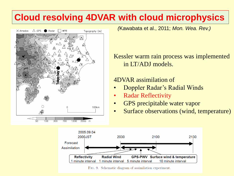
Kessler warm rain process was implemented

in LT/ADJ models.

4DVAR assimilation of

• Doppler Radar’s Radial Winds

• Radar Reflectivity

• GPS precipitable water vapor

• Surface observations (wind, temperature)

(Kawabata et al., 2011; Mon. Wea. Rev.)

Cloud resolving 4DVAR with cloud microphysics

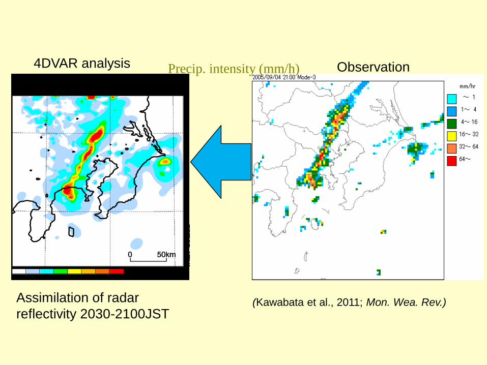
Precip. intensity (mm/h) 4DVAR analysis Observation

Assimilation of radar

reflectivity 2030-2100JST (Kawabata et al., 2011; Mon. Wea. Rev.)

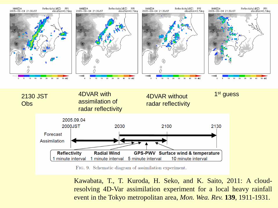
2130 JST

Obs

4DVAR with

assimilation of

radar reflectivity

4DVAR without

radar reflectivity

1st guess

Kawabata, T., T. Kuroda, H. Seko, and K. Saito, 2011: A cloud-

resolving 4D-Var assimilation experiment for a local heavy rainfall

event in the Tokyo metropolitan area, Mon. Wea. Rev. 139, 1911-1931.

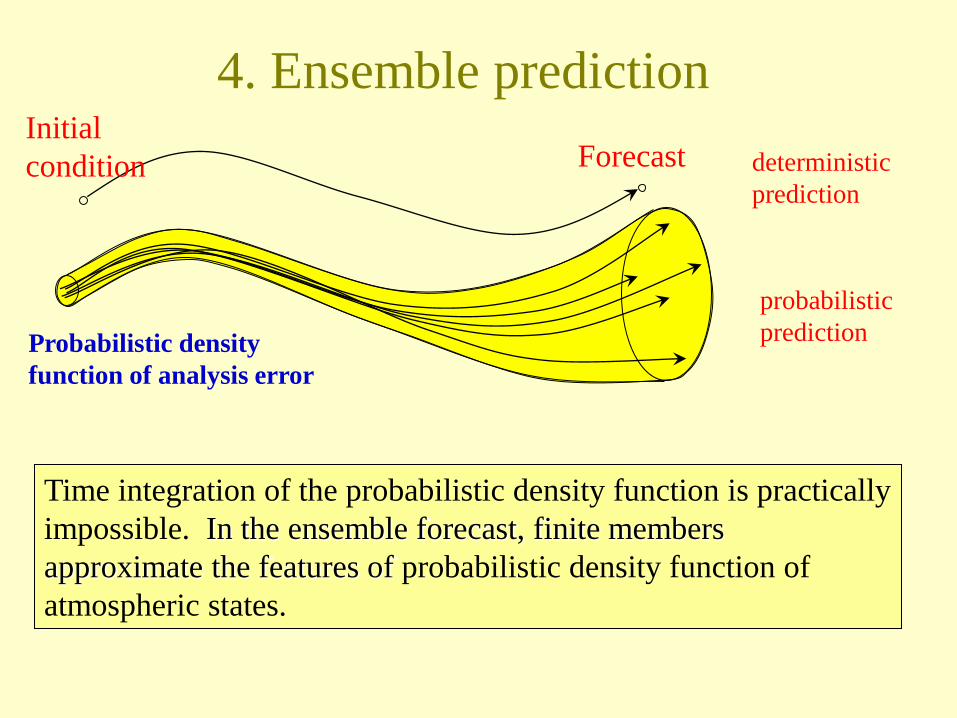
deterministic

prediction

probabilistic

prediction

Initial

condition Forecast

Probabilistic density

function of analysis error

Time integration of the probabilistic density function is practically

impossible. In the ensemble forecast, finite members

approximate the features of probabilistic density function of

atmospheric states.

4. Ensemble prediction

Forecast period

Forecast accuracy

2h 6hr 1day

Extrapolation


Nowcasting


precipitation



Reduce the gap

between nowcasting

and NWP by high-

resolution data

assimilation

Current NWP model

Approaches to predict local heavy rain

Forecast period

Forecast accuracy

2h 6hr 1day

Extrapolation


Nowcasting


precipitation



Reduce the gap

between nowcasting

and NWP by high-

resolution data

assimilation

Predictability by probabilistic forecast

Current NWP model

Ensemble forecast


2km ensemble prediction from JMA nonhydrostatic 4D-

VAR analysis for 2011 Niigata-Fukushima heavy rainfall

Control run Observation

03-06 UTC, 29 July 2011

Ensemble mean Ensemble spread

5mm/3h 10mm/3h 20mm/3h 50mm/3h

Probability of precipitation at FT=18

Solid probability even for 50mm/3h

1mm/3h

Saito et al. (2013)

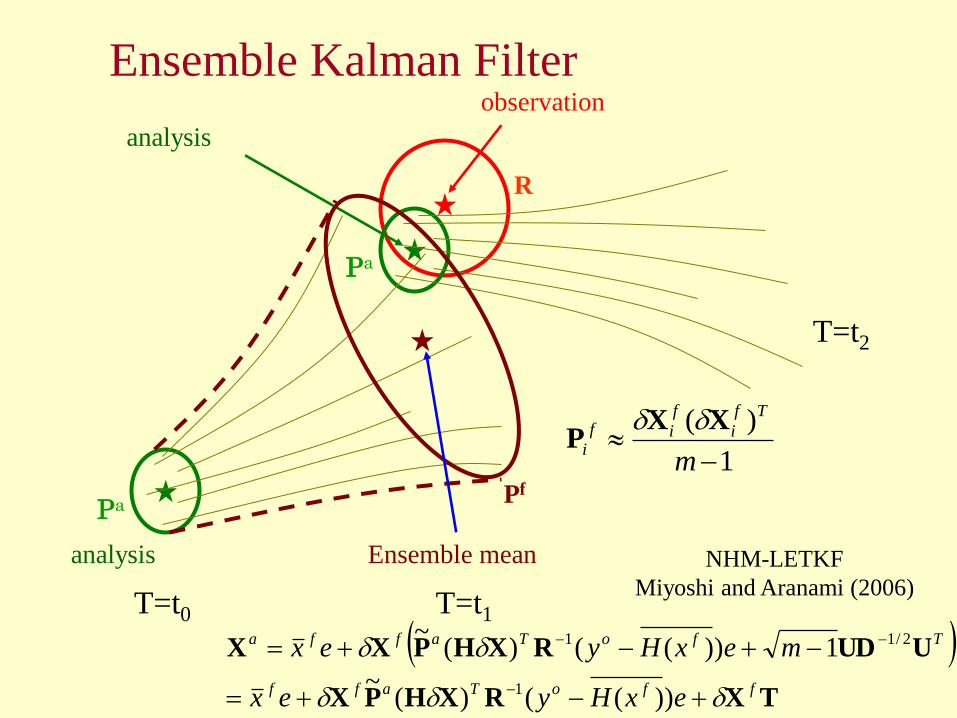
Ensemble Kalman Filter observation

analysis

T=t0 T=t1

NHM-LETKF

Miyoshi and Aranami (2006)

analysis Ensemble mean

Pf

T=t2

Pa

R

Pa

1

)(

m

Tf

i

f

if

i

XXP

TXRXHPX

UUDRXHPXX

ffoTaff

TfoTaffa

exHyex

mexHyex

))(()(~

1))(()(~

1

2/11

4. The K-Computer project

“HPCI Strategic Programs for Innovative Research (SPIRE)” is being

carried out by RIKEN, with partners in industry, universities, national

institutes under an initiative by MEXT

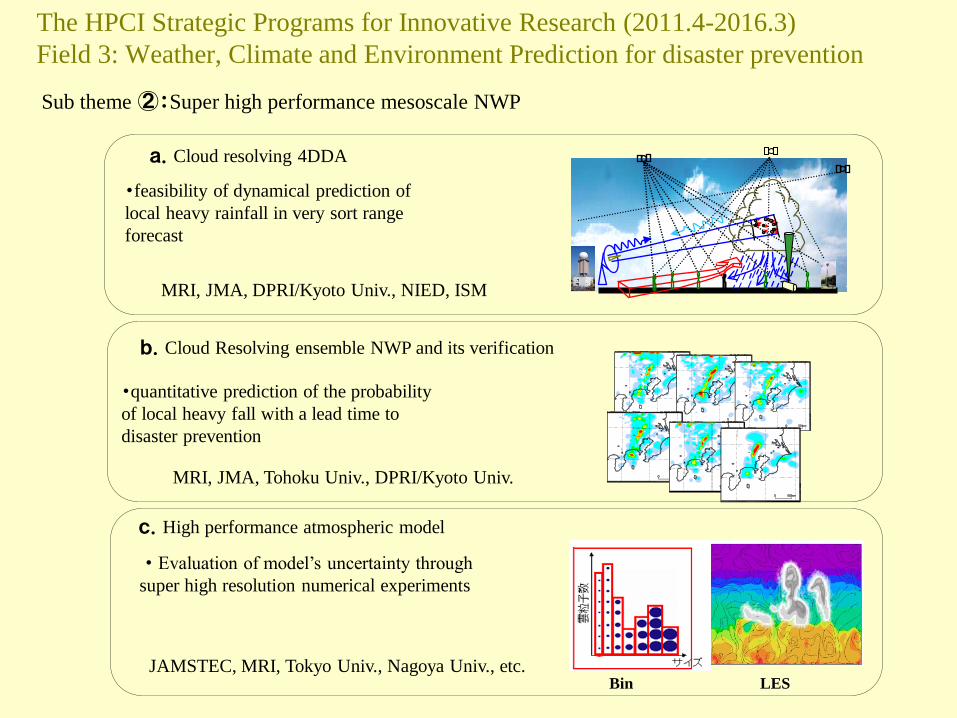
The HPCI Strategic Programs for Innovative Research (2011.4-2016.3)

Field 3: Weather, Climate and Environment Prediction for disaster prevention

Sub theme ②：Super high performance mesoscale NWP

ａ．Cloud resolving 4DDA

ｃ．High performance atmospheric model

ｂ．Cloud Resolving ensemble NWP and its verification

・feasibility of dynamical prediction of

local heavy rainfall in very sort range

forecast

・quantitative prediction of the probability

of local heavy fall with a lead time to

disaster prevention

・Evaluation of model’s uncertainty through

super high resolution numerical experiments

Bin LES

MRI, JMA, DPRI/Kyoto Univ., NIED, ISM

MRI, JMA, Tohoku Univ., DPRI/Kyoto Univ.

JAMSTEC, MRI, Tokyo Univ., Nagoya Univ., etc.

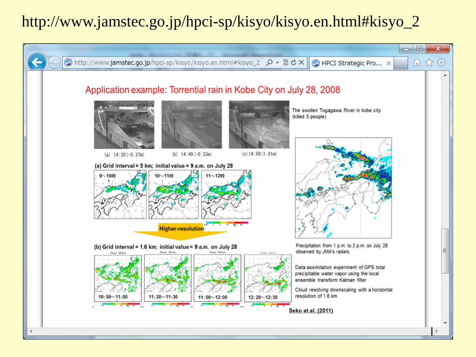
http://www.jamstec.go.jp/hpci-sp/kisyo/kisyo.en.html#kisyo_2

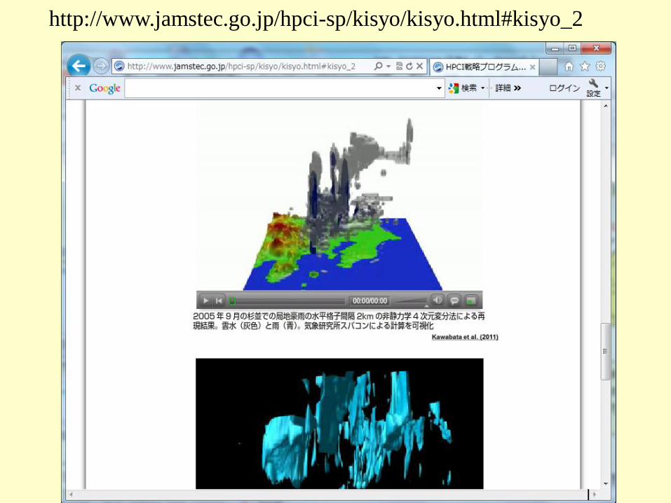
http://www.jamstec.go.jp/hpci-sp/kisyo/kisyo.html#kisyo_2

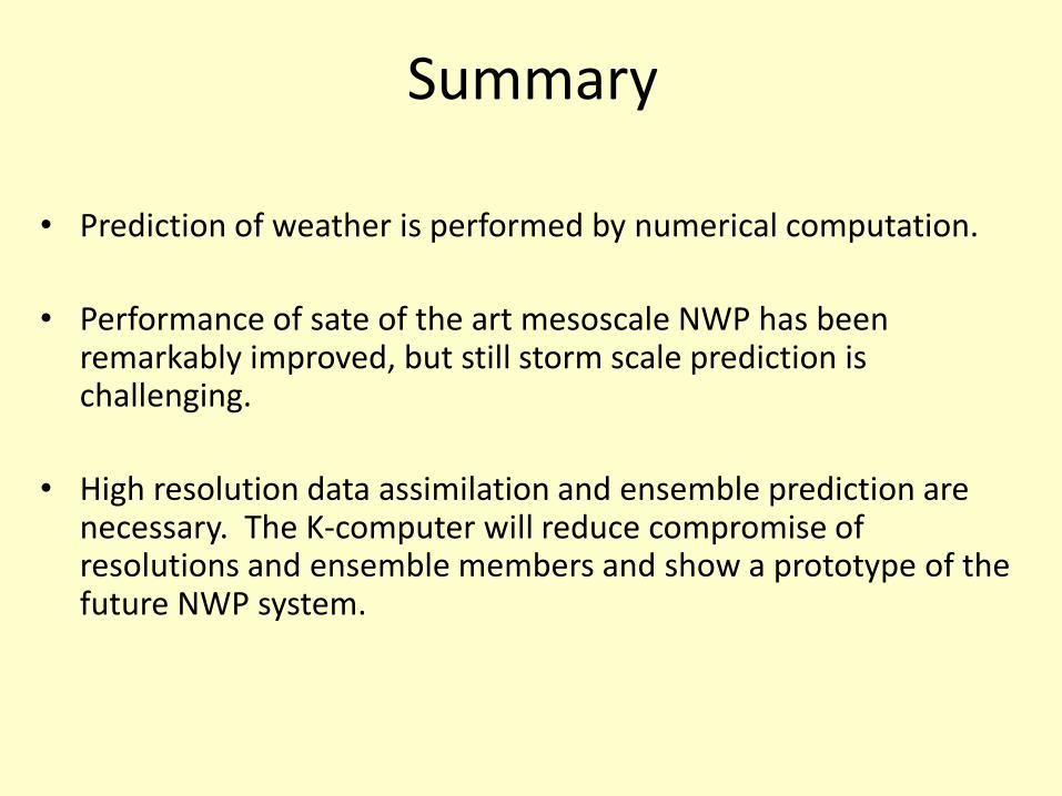
Summary

• Prediction of weather is performed by numerical computation.

• Performance of sate of the art mesoscale NWP has been remarkably improved, but still storm scale prediction is challenging.

• High resolution data assimilation and ensemble prediction are necessary. The K-computer will reduce compromise of resolutions and ensemble members and show a prototype of the future NWP system.

References Saito, K., T. Fujita, Y. Yamada, J. Ishida, Y. Kumagai, K. Aranami, S. Ohmori, R. Nagasawa, S. Kumagai, C. Muroi, T. Kato, H. Eito and Y.

Yamazaki, 2006: The operational JMA Nonhydrostatic Mesoscale Model. Mon. Wea. Rev., 134, 1266-1298.

Kawabata, T., H. Seko, K. Saito, T. Kuroda, K. Tamiya, T. Tsuyuki, Y. Honda and Y. Wakazuki, 2007: An Assimilation Experiment of the Nerima

Heavy Rainfall with a Cloud-Resolving Nonhydrostatic 4-Dimensional Variational Data Assimilation System. J. Meteor. Soc. Japan, 85, 255-

276.

Saito, K., J. Ishida, K. Aranami, T. Hara, T. Segawa, M. Narita and Y. Honda, 2007: Nonhydrostatic atmospheric models and operational

development at JMA. J. Meteor. Soc. Japan., 85B, 271-304.

Shoji, Y., M. Kunii and K. Saito, 2009: Assimilation of Nationwide and Global GPS PWV Data for a Heavy Rain Event on 28 July 2008 in

Hokuriku and Kinki, Japan. SOLA, 5, 45-48.

Kunii, M., K. Saito and H. Seko, 2010: Mesoscale Data Assimilation Experiment in the WWRP B08RDP. SOLA, 6, 33-36.

Saito, K., M. Kunii, M. Hara, H. Seko, T. Hara, M. Yamaguchi, T. Miyoshi and W. Wong, 2010: WWRP Beijing 2008 Olympics Forecast

Demonstration / Research and Development Project (B08FDP/RDP). Tech. Rep. MRI, 62, 210pp.

Seko, H., M. Kunii, Y. Shoji and K. Saito, 2010: Improvement of Rainfall Forecast by Assimilations of Ground-based GPS data and Radio

Occultation Data. SOLA. 6, 81-84.

Seko, H., T. Miyoshi, Y. Shoji and K. Saito, 2011: A data assimilation experiment of PWV using the LETKF system -Intense rainfall event on 28

July 2008-. Tellus, 63A, 402-414.

Saito, K., M. Hara, M. Kunii, H. Seko, and M. Yamaguchi, 2011: Comparison of initial perturbation methods for the mesoscale ensemble

prediction system of the Meteorological Research Institute for the WWRP Beijing 2008 Olympics Research and Development Project

(B08RDP). Tellus, 63A, 445-467.

Kunii, M., K. Saito, H. Seko, M. Hara, T. Hara, M. Yamaguchi, J. Gong, M. Charron, J. Du, Y. Wang and D. Chen, 2011: Verifications and

intercomparisons of mesoscale ensemble prediction systems in B08RDP. Tellus, 63A, 531-549.

Kawabata, T., T. Kuroda, H. Seko and K. Saito, 2011: A cloud-resolving 4D-Var assimilation experiment for a local heavy rainfall event in the

Tokyo metropolitan area. Mon. Wea. Rev., 139. 1911-1931.

Duan, Y., J. Gong, M. Charron, J. Chen, G. Deng, G. DiMego, J. Du, M. Hara, M. Kunii, X. Li , Y. Li, K. Saito, H. Seko, Y. Wang, and C.

Wittmann, 2011: An overview of Beijing 2008 Olympics Research and Development Project (B08RDP). Bull. Amer. Meteor. Soc. (in press)

Saito, K., H. Seko, M. Kunii and T. Miyoshi, 2012: Effect of lateral boundary perturbations on the breeding method and the local ensemble

transform Kalman filter for mesoscale ensemble prediction. Tellus. 64, doi:10.3402/tellusa.v64i0.11594.

Saito, K., 2012: JMA nonhydrostatic model. –Its application to operation and research. InTech. Atmospheric Model Applications, 85-110. doi:

10.5772/35368.

Seko, H., T. Tsuyuki, K. Saito and T. Miyoshi, 2012: Development of a two-way nested LETKF system for cloud resolving model. Springer. (in

press)

Duc, L., K. Saito and H. Seko, 2012: Spatial-Temporal Fractions Verification for High Resolution Ensemble Forecasts. Tellus. (submitted)

Thank you

Documents

Numerical Prediction of Mesoscale Weather for... · 2013-02-17 · Numerical Prediction of Mesoscale Weather 7th APEC - Tsukuba International Conference , 17 March 2013, Bunkyo School,