Embed Size (px)
Citation preview
Numerical simulation and benchmarking of amonolithic multigrid solver for fluid-structureinteraction problems with application tohemodynamics
S. Turek, J. Hron, M. Madlık, M. Razzaq, H. Wobker, and J. F. Acker
Abstract An Arbitrary Lagrangian-Eulerian (ALE) formulation is applied in a fullycoupled monolithic way, considering the fluid-structure interaction (FSI) problemas one continuum. The mathematical description and the numerical schemes aredesigned in such a way that general constitutive relations (which are realistic forbiomechanics applications) for the fluid as well as for the structural part can be eas-ily incorporated. We utilize the LBB-stable finite element pairs Q2P1 and P+
2 P1 fordiscretization in space to gain high accuracy and perform as time-stepping the 2ndorder Crank-Nicholson, respectively, a new modified Fractional-Step-θ -scheme forboth solid and fluid parts. The resulting discretized nonlinear algebraic system issolved by a Newton method which approximates the Jacobian matrices by a divideddifferences approach, and the resulting linear systems are solved by direct or itera-tive solvers, preferably of Krylov-multigrid type.For validation and evaluation of the accuracy and performance of the proposedmethodology, we present corresponding results for a new set of FSI benchmark con-figurations which describe the self-induced elastic deformation of a beam attachedto a cylinder in laminar channel flow, allowing stationary as well as periodicallyoscillating deformations. Then, as an example of FSI in biomedical problems, theinfluence of endovascular stent implantation on cerebral aneurysm hemodynamicsis numerically investigated. The aim is to study the interaction of the elastic wallsof the aneurysm with the geometrical shape of the implanted stent structure forprototypical 2D configurations. This study can be seen as a basic step towards theunderstanding of the resulting complex flow phenomena so that in future aneurysmrupture shall be suppressed by an optimal setting of the implanted stent geometry.
S. Turek, M. Razzaq, H. Wobker, J. F. AckerInstitute for Applied Mathematics, TU Dortmund, Vogelpothsweg 87, 44227 Dortmund, Germanye-mail: [email protected]
J. Hron, M. MadlıkMathematical Institute, Charles University Prague, Sokolovska 83, 18675 Prague, Czech republice-mail: [email protected]
1
2 S. Turek, J. Hron, M. Madlık, M. Razzaq, H. Wobker, and J. F. Acker
1 Introduction
In this paper, we consider the general problem of viscous flow interacting with anelastic body which is being deformed by the fluid action. Such a problem is of greatimportance in many real life applications, typical examples are the areas of biomed-ical fluids which include the influence of hemodynamic factors in blood vessels,cerebral aneurysm hemodynamics, joint lubrication and deformable cartilage, andblood flow interaction with elastic veins [2, 9, 25, 26, 34]. The theoretical investi-gation of fluid-structure interaction problems is complicated by the need of a mixeddescription for both parts: While for the solid part the natural view is the material(Lagrangian) description, for the fluid it is usually the spatial (Eulerian) description.In the case of their combination some kind of mixed description (usually referredto as the Arbitrary Lagrangian-Eulerian description or ALE) has to be used whichbrings additional nonlinearity into the resulting equations (see [17]).
The numerical solution of the resulting equations of the fluid-structure interactionproblem poses great challenges since it includes the features of structural mechan-ics, fluid dynamics, and their coupling. The most straightforward solution strategy,mostly used in the available software packages (see for instance [16]), is to decouplethe problem into the fluid part and solid part, for each of those parts using some wellestablished solution method; then the interaction process is introduced as externalboundary conditions in each of the subproblems. This has the advantage that thereare many well tested numerical methods for both separate problems of fluid flowand elastic deformation, while on the other hand the treatment of the interface andthe interaction is problematic due to high stiffness and sensitivity. In contrast, themonolithic approach discussed here treats the problem as a single continuum withthe coupling automatically taken care of as internal interface. This on the other handrequires more robust nonlinear and linear solvers for the global problem.
Besides a short description of the underlying numerical aspects regarding dis-cretization and solution procedure for this monolithic approach (see [17, 24]), wepresent corresponding results for a set of FSI benchmarking test cases (‘channelflow around cylinder with attached elastic beam’, see [30]), and we concentrate onprototypical numerical studies for 2D aneurysm configurations and first steps to-wards full 3D models. The corresponding parameterization is based on abstractionsof biomedical data (i.e., cutplanes of 3D specimens from New Zealand white rabbitsas well as computer tomographic and magnetic resonance imaging data of humanneurocrania). In our studies, we allow the walls of the aneurysm to be elastic andhence deforming with the flow field in the vessel. Moreover, we examine severalconfigurations for stent geometries which clearly influence the flow behavior insidethe aneurysm such that a very different elastic displacement of the walls is observed,too. We demonstrate that both the elastic modeling of the aneurysm walls as wellas the proper description of the geometrical details of the shape of the aneurysmand particularly of the stents are of great importance for a quantitative analysis ofthe complex interaction between structure and fluid. This is especially true in viewof more realistic blood flow models and anisotropic constitutive laws for the elasticwalls.
Numerical simulation and benchmarking of fluid-structure interaction 3
2 Fluid-structure interaction problem formulation
The general fluid-structure interaction problem consists of the description of thefluid and solid parts, appropriate interface conditions at the interface and conditionsfor the remaining boundaries, respectively. Here, we consider the flow of an incom-pressible Newtonian fluid interacting with an elastic solid. We denote the domainoccupied by the fluid by Ω
ft and the solid part by Ω s
t at the time t ∈ [0,T ]. LetΓ 0
t = Ωf
t ∩ Ω st be the part of the boundary where the elastic solid interacts with the
fluid. In the following, the description for both fields and the interface conditionsare introduced. Furthermore, discretization aspects and computational methods aredescribed.
2.1 Fluid mechanics
The fluid flow is assumed to be laminar. It can be described by the Navier-Stokesequations for incompressible flows
ρf (
∂v f
∂ t+v ·∇v)−∇ ·σ f = 0, ∇ ·v = 0 in Ω
ft (1)
where ρ f is the constant density. The state of the flow is described by the veloc-ity and pressure fields v f , p f , respectively. The external forces, for example dueto gravity or human motion, are assumed to be not significant and are neglected.Although the blood is known to be non-Newtonian in general, we assume it to beNewtonian in this study. This is because we consider large arteries with radii of morethan 2 mm, where the velocity and shear rate are high and the kinematic viscosityν f is nearly constant [20], such that the non-Newtonian effects can be neglected.The constitutive relation for the stress tensor reads
σf =−p f I+2µD(v f ), (2)
where µ is the dynamic viscosity of the fluid, p f is the Lagrange multiplier cor-responding to the incompressibility constraint in (1), and D(v f ) is the strain-ratetensor:
D(v f ) =12(∇v f +(∇v f )T ). (3)
For the fluid-structure interaction we use the ALE form of the balance equations.The corresponding discretization techniques are discussed in section 3. Let us re-mark that also non-Newtonian flow models can be used for modeling blood flow, forinstance of Power Law type or even including viscoelastic effects (see [7]) which isplanned for future extensions.
4 S. Turek, J. Hron, M. Madlık, M. Razzaq, H. Wobker, and J. F. Acker
2.2 Structural mechanics
The governing equations for the structural mechanics are the balance equations
ρs(
∂vs
∂ t+(∇vs)vs−g)−∇ ·σ s = 0, in Ω
st , (4)
where the superscript s denotes the structure, ρs is the density of the material, gs
represents the external body forces acting on the structure, and σ s is the Cauchystress tensor. The deformation of the structure is described by the displacement us,with velocity field vs = ∂us
∂ t . Written in the more common Lagrangian description,i.e. with respect to some fixed reference (for example initial) state Ω s, we have
ρs0(
∂ 2us
∂ t2 −g)−∇ ·Σs = 0, in Ωs, (5)
where Σs = Jσ sF−T is the first Piola-Kirchhoff stress tensor. J denotes the deter-minant of the deformation gradient tensor F, defined as F = I + ∇us. Unlike theCauchy stress tensor σ s, Σs is non-symmetric. Since constitutive relations are oftenexpressed in terms of symmetric stress tensor, it is natural to introduce the secondPiola-Kirchhoff tensor Ss
Ss = F−T Σs = JF−1σ
sF−T , (6)
which is symmetric. For elastic material the stress is a function of the deformation(and possibly of thermodynamic variables such as the temperature) but it is inde-pendent of deformation history and thus of time. The material characteristics maystill vary in space. In a homogeneous material mechanical properties do not vary, thestrain energy function depends only on the deformation. A material is mechanicallyisotropic if its response to deformation is the same in all directions. The constitutiveequation is then a function of F. More precisely, it is usually written in terms of theGreen-Lagrange strain tensor, as
E =12(C− I), (7)
where I is the identity tensor and C = FT F is the left Cauchy-Green strain tensor.For the subsequent FSI benchmark calculations we employ the St. Venant-Kirch-
hoff material model as an example for homogeneous isotropic material whose ref-erence configuration is the natural state (i.e. where the Cauchy stress tensor is zeroeverywhere). The St. Venant-Kirchhoff material model is specified by the followingconstitutive law
σs =
1J
F(λ s(trE)I+2µsE)FT Ss = λ
s(trE)I+2µsE, (8)
Numerical simulation and benchmarking of fluid-structure interaction 5
where λ s denotes the first Lame coefficient, and µs the shear modulus. More com-plex constitutive relations for hyperelastic materials may be found in [14], and par-ticular models for biological tissues and blood vessels are reported in [11, 15]. Thematerial elasticity is characterized by a set of two parameters, the Poisson ratio νs
and the Young modulus E. These parameters satisfy the relations
νs =
λ s
2(λ s + µs)E =
µs(3λ s +2µ2)(λ s + µs)
(9)
µs =
E2(1+νs)
λs =
νsE(1+νs)(1−2νs)
, (10)
where νs = 1/2 for incompressible and νs < 1/2 for compressible material. In thelarge deformation case it is common to describe the constitutive equation using astress-strain relation based on the Green Lagrange strain tensor E and the secondPiola-Kirchhoff stress tensor S(E) as a function of E. However, also incompressiblematerials can be handled in the same way (see [17]).
For the hemodynamic applications, a Neo-Hooke material model is taken whichcan be used for compressible or incompressible (for νs→ 1/2⇒ λ s→∞ ) materialand which is described by the constitutive laws:
σs =−psI+
µs
J(FFT − I) (11)
0 =−ps +λ s
2(J− 1
J) (12)
Both models, the St. Venant-Kirchhoff and the Neo-Hooke material model, sharethe isotropic and homogenous properties, and both can be used for the computationof large deformations. However, the St. Venant-Kirchhoff model does not allow forlarge strain computation, while the Neo-Hooke model is also valid for large strains.In the case of small strains and small deformations, both material laws yield thesame linearized material model. We implemented the St. Venant-Kirchhoff mate-rial model as the standard model for the compressible case, since the setup of thebenchmark does not involve large strains in the oscillating beam structure. Its imple-mentation is simpler and, therefore, the FSI benchmark will hopefully be adoptedby a wider group of researchers. If someone wants or has to use the Neo-Hookematerial, the results for a given set of E and ν or λ and µ are comparable, if thestandard Neo-Hooke material model as in (11), (12) is used. Similarly as in the caseof more complex blood flow models, also more realistic constitutive relations forthe anisotropic behavior of the walls of aneurysms can be included which howeveris beyond the scope of this paper.
6 S. Turek, J. Hron, M. Madlık, M. Razzaq, H. Wobker, and J. F. Acker
2.3 Interaction conditions
The boundary conditions on the fluid-solid interface are assumed to be
σf n = σ
sn, v f = vs, on Γ0
t , (13)
where n is a unit normal vector to the interface Γ 0t . This implies the no-slip condition
for the flow and that the forces on the interface are in balance.
3 Discretization and solution techniques
For the moment, we restrict our considerations to two dimensions which allows sys-tematic tests of the proposed methods for biomedical applications in a very efficientway such that the qualitatitive behavior can be carefully analyzed. The correspond-ing fully implicit, monolithic treatment of the fluid-structure interaction problemsuggests that an A-stable second order time stepping scheme and that the same finiteelements for both the solid part and the fluid region should be utilized. Moreover,to handle the fluid incompressibility constraints, we have to choose a stable finiteelement pair. For that reason, the conforming biquadratic, discontinuous linear Q2P1pair is used. Let us define the usual finite dimensional spaces U for displacement, Vfor velocity, P for pressure approximation as follows
U = u ∈ L∞(I, [W 1,2(Ω)]2),u = 0 on ∂Ω,V = v ∈ L2(I, [W 1,2(Ωt)]2)∩L∞(I, [L2(Ωt)]2),v = 0 on ∂Ω,P = p ∈ L2(I,L2(Ω)).
Then the variational formulation of the fluid-structure interaction problem is tofind (u,v, p) ∈U ×V ×P that satisfy the corresponding weak form of the balanceequations including appropriate initial conditions. The spaces U,V,P on an interval[tn, tn+1] would be approximated in the case of the Q2,P1 pair as
Uh = uh ∈ [C(Ωh)]2,uh|T ∈ [Q2(T )]2 ∀T ∈Th,uh = 0 on ∂Ωh,Vh = vh ∈ [C(Ωh)]2,vh|T ∈ [Q2(T )]2 ∀T ∈Th,vh = 0 on ∂Ωh,Ph = ph ∈ L2(Ωh), ph|T ∈ P1(T ) ∀T ∈Th.
Let us denote by unh the approximation of u(tn), vn
h the approximation of v(tn) andpn
h the approximation of p(tn). Consider for each T ∈Th the bilinear transformationψT : T → T , where T is the unit square. Then, Q2(T ) is defined as
Q2(T ) =
qψ−1T : q ∈ span < 1,x,y,xy,x2,y2,x2y,y2x,x2y2 >
(14)
Numerical simulation and benchmarking of fluid-structure interaction 7
with nine local degrees of freedom located at the vertices, midpoints of the edgesand in the center of the quadrilateral. The space P1(T ) consists of linear functionsdefined by
P1(T ) =
qψ−1T : q ∈ span < 1,x,y >
(15)
with the function value and both partial derivatives located in the center of thequadrilateral, as its three local degrees of freedom, which leads to a discontinu-ous pressure. The inf-sup condition is satisfied (see [5]); however, the combinationof the bilinear transformation ψ with a linear function on the reference square P1(T )would imply that the basis on the reference square did not contain the full basis. So,the method can at most be first order accurate on general meshes (see [3, 5])
‖p− ph‖0 = O(h). (16)
The standard remedy is to consider a local coordinate system (ξ ,η) obtained byjoining the midpoints of the opposing faces of T (see [3, 22, 29]). Then, we set oneach element T
P1(T ) := span < 1,ξ ,η > . (17)
For this case, the inf-sup condition is also satisfied and the second order approxima-tion is recovered for the pressure as well as for the velocity gradient (see [5, 13])
‖p− ph‖0 = O(h2) and ‖∇(u−uh)‖0 = O(h2). (18)
For a smooth solution, the approximation error for the velocity in the L2-norm isof order O(h3) which can easily be demonstrated for prescribed polynomials or forsmooth data on appropriate domains.
In the last section we present first results for 3-dimensional computation wherewe use the P+
2 P1 pair which also satisfies the Babuska–Brezzi stability conditionand yields a stable discretization of the incompressible problems (see [10]).
3.1 Time discretization
In view of a more compact presentation, the applied time discretization approachis described only for the fluid part (see [23] for more details). In the following, werestrict to the (standard) incompressible Navier-Stokes equations
vt −ν∆v+v ·∇v+∇p = f, ∇ ·v = 0, in Ω × (0,T ] , (19)
for given force f and viscosity ν , with prescribed boundary values on the boundary∂Ω and an initial condition at t = 0.
8 S. Turek, J. Hron, M. Madlık, M. Razzaq, H. Wobker, and J. F. Acker
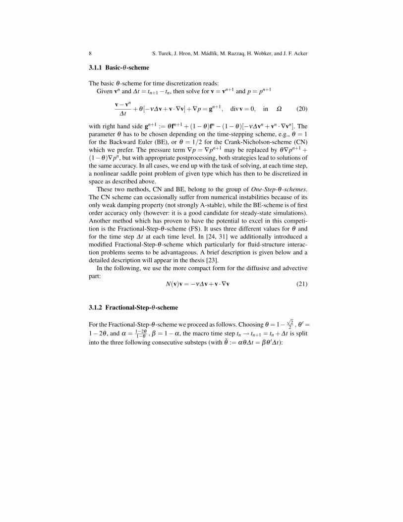
3.1.1 Basic-θ -scheme
The basic θ -scheme for time discretization reads:Given vn and ∆ t = tn+1− tn, then solve for v = vn+1 and p = pn+1
v−vn
∆ t+θ [−ν∆v+v ·∇v]+∇p = gn+1, divv = 0, in Ω (20)
with right hand side gn+1 := θ fn+1 +(1− θ)fn− (1− θ)[−ν∆vn + vn ·∇vn]. Theparameter θ has to be chosen depending on the time-stepping scheme, e.g., θ = 1for the Backward Euler (BE), or θ = 1/2 for the Crank-Nicholson-scheme (CN)which we prefer. The pressure term ∇p = ∇pn+1 may be replaced by θ∇pn+1 +(1−θ)∇pn, but with appropriate postprocessing, both strategies lead to solutions ofthe same accuracy. In all cases, we end up with the task of solving, at each time step,a nonlinear saddle point problem of given type which has then to be discretized inspace as described above.
These two methods, CN and BE, belong to the group of One-Step-θ -schemes.The CN scheme can occasionally suffer from numerical instabilities because of itsonly weak damping property (not strongly A-stable), while the BE-scheme is of firstorder accuracy only (however: it is a good candidate for steady-state simulations).Another method which has proven to have the potential to excel in this competi-tion is the Fractional-Step-θ -scheme (FS). It uses three different values for θ andfor the time step ∆ t at each time level. In [24, 31] we additionally introduced amodified Fractional-Step-θ -scheme which particularly for fluid-structure interac-tion problems seems to be advantageous. A brief description is given below and adetailed description will appear in the thesis [23].
In the following, we use the more compact form for the diffusive and advectivepart:
N(v)v =−ν∆v+v ·∇v (21)
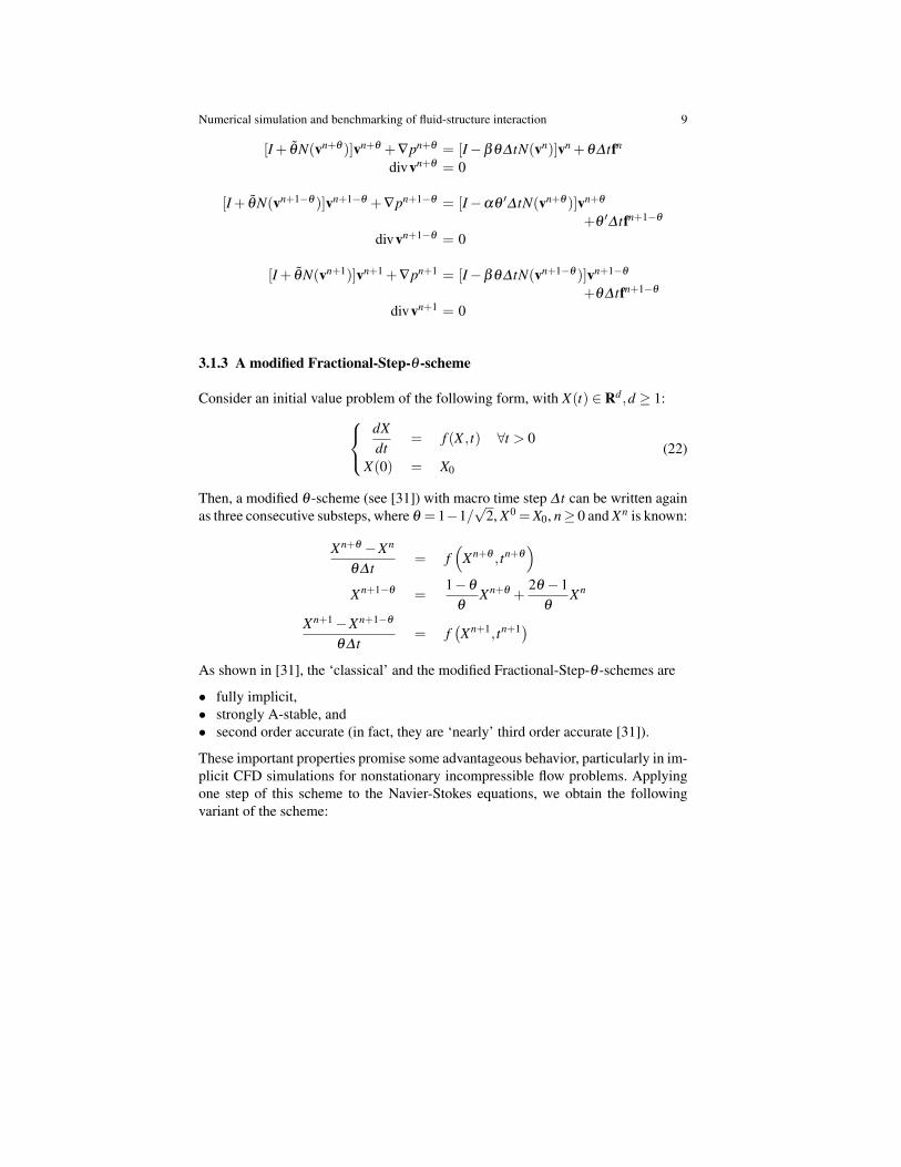
3.1.2 Fractional-Step-θ -scheme
For the Fractional-Step-θ -scheme we proceed as follows. Choosing θ = 1−√
22 , θ ′=
1−2θ , and α = 1−2θ
1−θ, β = 1−α , the macro time step tn→ tn+1 = tn + ∆ t is split
into the three following consecutive substeps (with θ := αθ∆ t = βθ ′∆ t):
Numerical simulation and benchmarking of fluid-structure interaction 9
[I + θN(vn+θ )]vn+θ +∇pn+θ = [I−βθ∆ tN(vn)]vn +θ∆ tfn
divvn+θ = 0
[I + θN(vn+1−θ )]vn+1−θ +∇pn+1−θ = [I−αθ ′∆ tN(vn+θ )]vn+θ
+θ ′∆ tfn+1−θ
divvn+1−θ = 0
[I + θN(vn+1)]vn+1 +∇pn+1 = [I−βθ∆ tN(vn+1−θ )]vn+1−θ
+θ∆ tfn+1−θ
divvn+1 = 0
3.1.3 A modified Fractional-Step-θ -scheme
Consider an initial value problem of the following form, with X(t) ∈ Rd ,d ≥ 1:dXdt
= f (X , t) ∀t > 0
X(0) = X0
(22)
Then, a modified θ -scheme (see [31]) with macro time step ∆ t can be written againas three consecutive substeps, where θ = 1−1/
√2, X0 = X0, n≥ 0 and Xn is known:
Xn+θ −Xn
θ∆ t= f
(Xn+θ , tn+θ
)Xn+1−θ =
1−θ
θXn+θ +
2θ −1θ
Xn
Xn+1−Xn+1−θ
θ∆ t= f
(Xn+1, tn+1)
As shown in [31], the ‘classical’ and the modified Fractional-Step-θ -schemes are
• fully implicit,• strongly A-stable, and• second order accurate (in fact, they are ‘nearly’ third order accurate [31]).
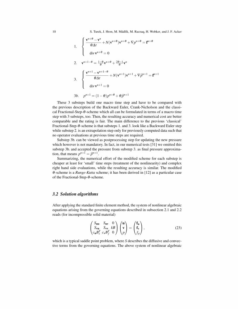
These important properties promise some advantageous behavior, particularly in im-plicit CFD simulations for nonstationary incompressible flow problems. Applyingone step of this scheme to the Navier-Stokes equations, we obtain the followingvariant of the scheme:
10 S. Turek, J. Hron, M. Madlık, M. Razzaq, H. Wobker, and J. F. Acker
1.
vn+θ −vn
θ∆ t+N(vn+θ )vn+θ +∇pn+θ = fn+θ
divvn+θ = 0
2. vn+1−θ = 1−θ
θvn+θ + 2θ−1
θvn
3.
vn+1−vn+1−θ
θ∆ t+N(vn+1)vn+1 +∇pn+1 = fn+1
divvn+1 = 0
3b. pn+1 = (1−θ)pn+θ +θ pn+1
These 3 substeps build one macro time step and have to be compared withthe previous description of the Backward Euler, Crank-Nicholson and the classi-cal Fractional-Step-θ -scheme which all can be formulated in terms of a macro timestep with 3 substeps, too. Then, the resulting accuracy and numerical cost are bettercomparable and the rating is fair. The main difference to the previous ‘classical’Fractional-Step-θ -scheme is that substeps 1. and 3. look like a Backward Euler stepwhile substep 2. is an extrapolation step only for previously computed data such thatno operator evaluations at previous time steps are required.
Substep 3b. can be viewed as postprocessing step for updating the new pressurewhich however is not mandatory. In fact, in our numerical tests [31] we omitted thissubstep 3b. and accepted the pressure from substep 3. as final pressure approxima-tion, that means pn+1 = pn+1.
Summarizing, the numerical effort of the modified scheme for each substep ischeaper at least for ‘small’ time steps (treatment of the nonlinearity) and complexright hand side evaluations, while the resulting accuracy is similar. The modifiedθ -scheme is a Runge-Kutta scheme; it has been derived in [12] as a particular caseof the Fractional-Step-θ -scheme.
3.2 Solution algorithms
After applying the standard finite element method, the system of nonlinear algebraicequations arising from the governing equations described in subsection 2.1 and 2.2reads (for incompressible solid material) Suu Suv 0
Svu Svv kBcuBT
s cvBTf 0
uvp
=
fufvfp
, (23)
which is a typical saddle point problem, where S describes the diffusive and convec-tive terms from the governing equations. The above system of nonlinear algebraic
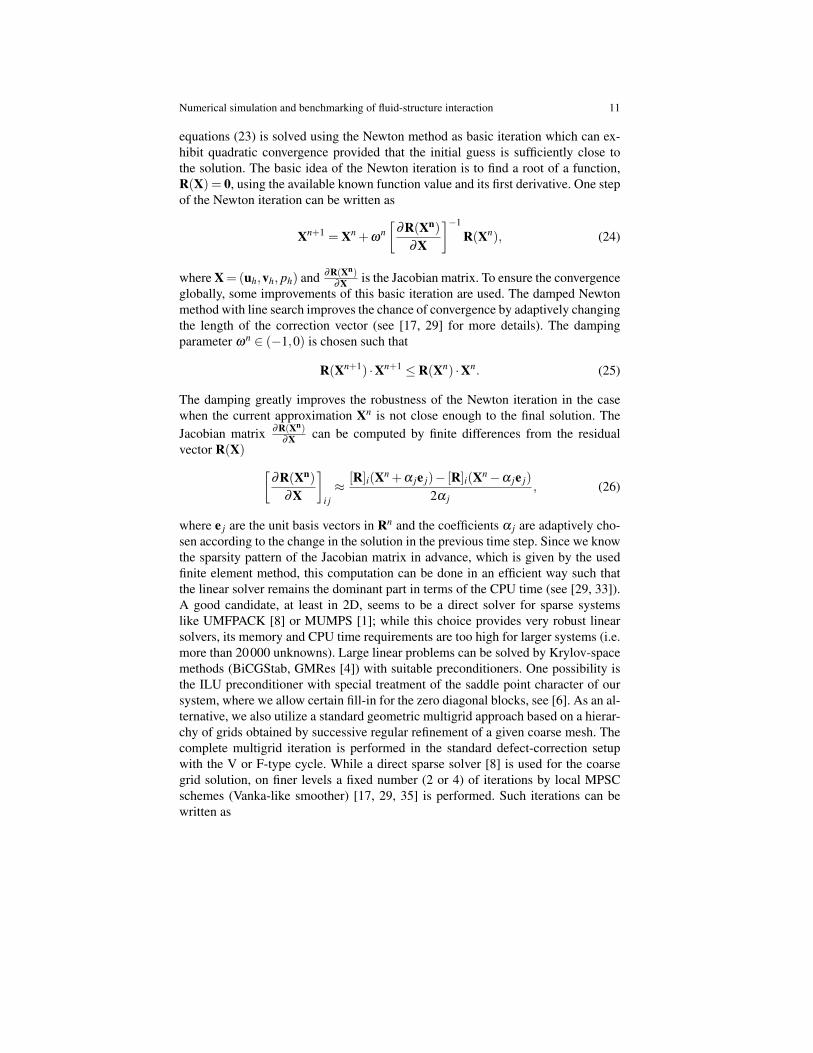
Numerical simulation and benchmarking of fluid-structure interaction 11
equations (23) is solved using the Newton method as basic iteration which can ex-hibit quadratic convergence provided that the initial guess is sufficiently close tothe solution. The basic idea of the Newton iteration is to find a root of a function,R(X) = 0, using the available known function value and its first derivative. One stepof the Newton iteration can be written as
Xn+1 = Xn +ωn[
∂R(Xn)∂X
]−1
R(Xn), (24)
where X = (uh,vh, ph) and ∂R(Xn)∂X is the Jacobian matrix. To ensure the convergence
globally, some improvements of this basic iteration are used. The damped Newtonmethod with line search improves the chance of convergence by adaptively changingthe length of the correction vector (see [17, 29] for more details). The dampingparameter ωn ∈ (−1,0) is chosen such that
R(Xn+1) ·Xn+1 ≤ R(Xn) ·Xn. (25)
The damping greatly improves the robustness of the Newton iteration in the casewhen the current approximation Xn is not close enough to the final solution. TheJacobian matrix ∂R(Xn)
∂X can be computed by finite differences from the residualvector R(X) [
∂R(Xn)∂X
]i j≈
[R]i(Xn +α je j)− [R]i(Xn−α je j)2α j
, (26)
where e j are the unit basis vectors in Rn and the coefficients α j are adaptively cho-sen according to the change in the solution in the previous time step. Since we knowthe sparsity pattern of the Jacobian matrix in advance, which is given by the usedfinite element method, this computation can be done in an efficient way such thatthe linear solver remains the dominant part in terms of the CPU time (see [29, 33]).A good candidate, at least in 2D, seems to be a direct solver for sparse systemslike UMFPACK [8] or MUMPS [1]; while this choice provides very robust linearsolvers, its memory and CPU time requirements are too high for larger systems (i.e.more than 20000 unknowns). Large linear problems can be solved by Krylov-spacemethods (BiCGStab, GMRes [4]) with suitable preconditioners. One possibility isthe ILU preconditioner with special treatment of the saddle point character of oursystem, where we allow certain fill-in for the zero diagonal blocks, see [6]. As an al-ternative, we also utilize a standard geometric multigrid approach based on a hierar-chy of grids obtained by successive regular refinement of a given coarse mesh. Thecomplete multigrid iteration is performed in the standard defect-correction setupwith the V or F-type cycle. While a direct sparse solver [8] is used for the coarsegrid solution, on finer levels a fixed number (2 or 4) of iterations by local MPSCschemes (Vanka-like smoother) [17, 29, 35] is performed. Such iterations can bewritten as
12 S. Turek, J. Hron, M. Madlık, M. Razzaq, H. Wobker, and J. F. Ackerul+1
vl+1
pl+1
=
ul
vl
pl
−ω ∑elementΩi
Suu|Ωi Suv|Ωi 0Svu|Ωi Svv|Ωi kB|Ωi
cuBTs|Ωi
cvBTf |Ωi
0
−1deflu
deflv
de f lp
.
The inverse of the local (39×39) systems can be computed by hardware optimizeddirect solvers. The full nodal interpolation is used as the prolongation operator Pwith its transposed operator used as the restriction R = PT , see [16, 29] for moredetails.
4 FSI benchmarking
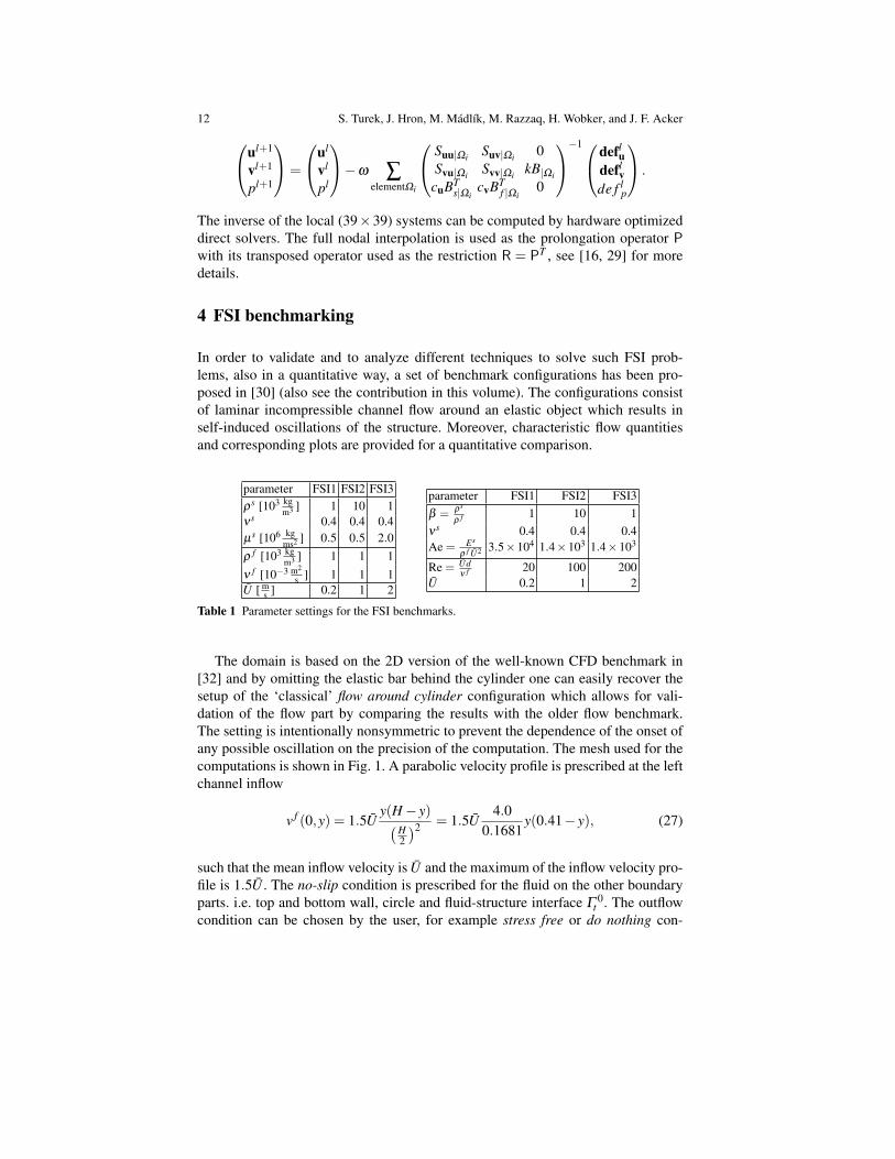
In order to validate and to analyze different techniques to solve such FSI prob-lems, also in a quantitative way, a set of benchmark configurations has been pro-posed in [30] (also see the contribution in this volume). The configurations consistof laminar incompressible channel flow around an elastic object which results inself-induced oscillations of the structure. Moreover, characteristic flow quantitiesand corresponding plots are provided for a quantitative comparison.
parameter FSI1 FSI2 FSI3ρs [103 kg
m3 ] 1 10 1νs 0.4 0.4 0.4µs [106 kg
ms2 ] 0.5 0.5 2.0ρ f [103 kg
m3 ] 1 1 1ν f [10−3 m2
s ] 1 1 1U [ m
s ] 0.2 1 2
parameter FSI1 FSI2 FSI3β = ρs
ρ f 1 10 1νs 0.4 0.4 0.4Ae = Es
ρ f U2 3.5×10⁴ 1.4×10³ 1.4×10³
Re = Udν f 20 100 200
U 0.2 1 2
Table 1 Parameter settings for the FSI benchmarks.
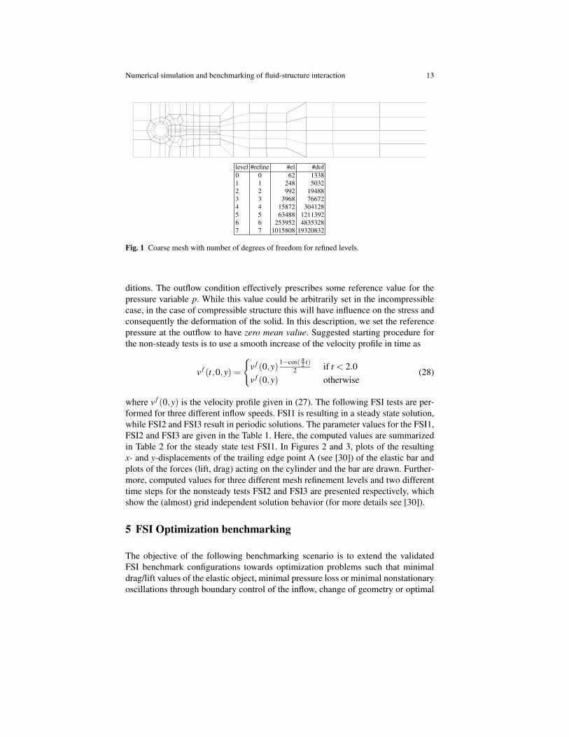
The domain is based on the 2D version of the well-known CFD benchmark in[32] and by omitting the elastic bar behind the cylinder one can easily recover thesetup of the ‘classical’ flow around cylinder configuration which allows for vali-dation of the flow part by comparing the results with the older flow benchmark.The setting is intentionally nonsymmetric to prevent the dependence of the onset ofany possible oscillation on the precision of the computation. The mesh used for thecomputations is shown in Fig. 1. A parabolic velocity profile is prescribed at the leftchannel inflow
v f (0,y) = 1.5Uy(H− y)(H
2
)2 = 1.5U4.0
0.1681y(0.41− y), (27)
such that the mean inflow velocity is U and the maximum of the inflow velocity pro-file is 1.5U . The no-slip condition is prescribed for the fluid on the other boundaryparts. i.e. top and bottom wall, circle and fluid-structure interface Γ 0
t . The outflowcondition can be chosen by the user, for example stress free or do nothing con-
Numerical simulation and benchmarking of fluid-structure interaction 13
level #refine #el #dof0 0 62 13381 1 248 50322 2 992 194883 3 3968 766724 4 15872 3041285 5 63488 12113926 6 253952 48353287 7 1015808 19320832
Fig. 1 Coarse mesh with number of degrees of freedom for refined levels.
ditions. The outflow condition effectively prescribes some reference value for thepressure variable p. While this value could be arbitrarily set in the incompressiblecase, in the case of compressible structure this will have influence on the stress andconsequently the deformation of the solid. In this description, we set the referencepressure at the outflow to have zero mean value. Suggested starting procedure forthe non-steady tests is to use a smooth increase of the velocity profile in time as
v f (t,0,y) =
v f (0,y) 1−cos( π
2 t)2 if t < 2.0
v f (0,y) otherwise(28)
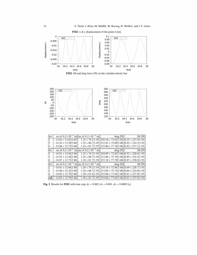
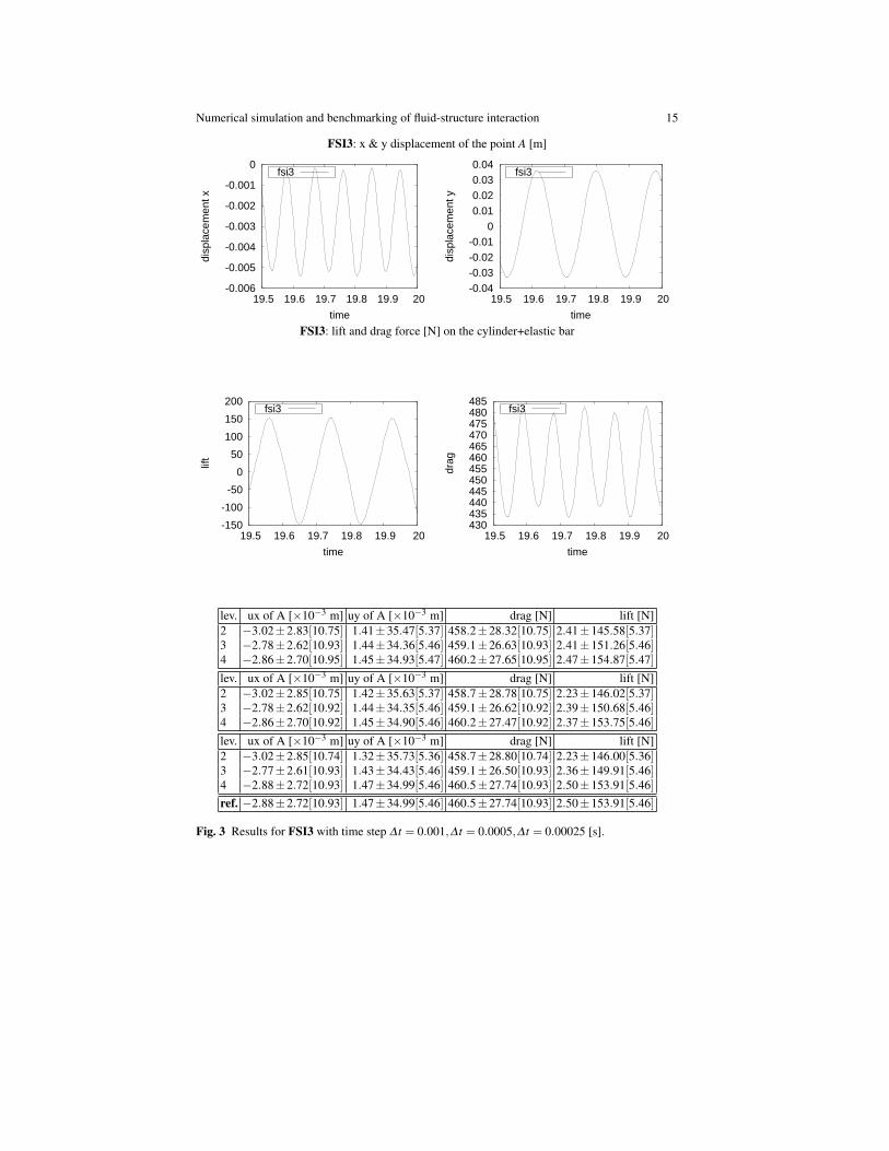
where v f (0,y) is the velocity profile given in (27). The following FSI tests are per-formed for three different inflow speeds. FSI1 is resulting in a steady state solution,while FSI2 and FSI3 result in periodic solutions. The parameter values for the FSI1,FSI2 and FSI3 are given in the Table 1. Here, the computed values are summarizedin Table 2 for the steady state test FSI1. In Figures 2 and 3, plots of the resultingx- and y-displacements of the trailing edge point A (see [30]) of the elastic bar andplots of the forces (lift, drag) acting on the cylinder and the bar are drawn. Further-more, computed values for three different mesh refinement levels and two differenttime steps for the nonsteady tests FSI2 and FSI3 are presented respectively, whichshow the (almost) grid independent solution behavior (for more details see [30]).
5 FSI Optimization benchmarking
The objective of the following benchmarking scenario is to extend the validatedFSI benchmark configurations towards optimization problems such that minimaldrag/lift values of the elastic object, minimal pressure loss or minimal nonstationaryoscillations through boundary control of the inflow, change of geometry or optimal
14 S. Turek, J. Hron, M. Madlık, M. Razzaq, H. Wobker, and J. F. Acker
FSI2: x & y displacement of the point A [m].
-0.03
-0.025
-0.02
-0.015
-0.01
-0.005
0
34 34.2 34.4 34.6 34.8 35
disp
lace
men
t x
time
fsi2
-0.08-0.06-0.04-0.02
0 0.02 0.04 0.06 0.08 0.1
34 34.2 34.4 34.6 34.8 35
disp
lace
men
t y
time
fsi2
FSI2: lift and drag force [N] on the cylinder+elastic bar.
-250-200-150-100-50
0 50
100 150 200 250
34 34.2 34.4 34.6 34.8 35
lift
time
fsi2
120 140 160 180 200 220 240 260 280 300
34 34.2 34.4 34.6 34.8 35
drag
time
fsi2
lev. ux of A [×10−3 m] uy of A [×10−3 m] drag [N] lift [N]2 −14.02±12.03[3.85] 1.25±79.3[1.93] 210.10±72.62[3.85] 0.25±227.9[1.93]3 −14.54±12.50[3.86] 1.25±80.7[1.93] 212.83±75.89[3.86] 0.92±234.3[1.93]4 −14.88±12.75[3.86] 1.24±81.7[1.93] 215.06±77.76[3.86] 0.82±237.1[1.93]lev. ux of A [×10−3 m] uy of A [×10−3 m] drag [N] lift [N]2 −14.01±12.04[3.86] 1.25±79.3[1.93] 210.09±72.82[3.86] 0.52±228.6[1.93]3 −14.54±12.48[3.86] 1.25±80.7[1.93] 213.06±75.76[3.86] 0.85±234.4[1.93]4 −14.87±12.73[3.86] 1.24±81.7[1.93] 215.18±77.78[3.86] 0.87±238.0[1.93]lev. ux of A [×10−3 m] uy of A [×10−3 m] drag [N] lift [N]2 −14.01±12.04[3.86] 1.28±79.2[1.93] 210.14±72.86[3.86] 0.49±228.7[1.93]3 −14.48±12.45[3.86] 1.24±80.7[1.93] 213.05±75.74[3.86] 0.84±234.8[1.93]4 −14.85±12.70[3.86] 1.30±81.6[1.93] 215.06±77.65[3.86] 0.61±237.8[1.93]ref. −14.85±12.70[3.86] 1.30±81.7[1.93] 215.06±77.65[3.86] 0.61±237.8[1.93]
Fig. 2 Results for FSI2 with time step ∆ t = 0.002,∆ t = 0.001,∆ t = 0.0005 [s].
Numerical simulation and benchmarking of fluid-structure interaction 15
FSI3: x & y displacement of the point A [m]
-0.006
-0.005
-0.004
-0.003
-0.002
-0.001
0
19.5 19.6 19.7 19.8 19.9 20
disp
lace
men
t x
time
fsi3
-0.04-0.03-0.02-0.01
0 0.01 0.02 0.03 0.04
19.5 19.6 19.7 19.8 19.9 20
disp
lace
men
t y
time
fsi3
FSI3: lift and drag force [N] on the cylinder+elastic bar
-150
-100
-50
0
50
100
150
200
19.5 19.6 19.7 19.8 19.9 20
lift
time
fsi3
430 435 440 445 450 455 460 465 470 475 480 485
19.5 19.6 19.7 19.8 19.9 20
drag
time
fsi3
lev. ux of A [×10−3 m] uy of A [×10−3 m] drag [N] lift [N]2 −3.02±2.83[10.75] 1.41±35.47[5.37] 458.2±28.32[10.75] 2.41±145.58[5.37]3 −2.78±2.62[10.93] 1.44±34.36[5.46] 459.1±26.63[10.93] 2.41±151.26[5.46]4 −2.86±2.70[10.95] 1.45±34.93[5.47] 460.2±27.65[10.95] 2.47±154.87[5.47]lev. ux of A [×10−3 m] uy of A [×10−3 m] drag [N] lift [N]2 −3.02±2.85[10.75] 1.42±35.63[5.37] 458.7±28.78[10.75] 2.23±146.02[5.37]3 −2.78±2.62[10.92] 1.44±34.35[5.46] 459.1±26.62[10.92] 2.39±150.68[5.46]4 −2.86±2.70[10.92] 1.45±34.90[5.46] 460.2±27.47[10.92] 2.37±153.75[5.46]lev. ux of A [×10−3 m] uy of A [×10−3 m] drag [N] lift [N]2 −3.02±2.85[10.74] 1.32±35.73[5.36] 458.7±28.80[10.74] 2.23±146.00[5.36]3 −2.77±2.61[10.93] 1.43±34.43[5.46] 459.1±26.50[10.93] 2.36±149.91[5.46]4 −2.88±2.72[10.93] 1.47±34.99[5.46] 460.5±27.74[10.93] 2.50±153.91[5.46]ref. −2.88±2.72[10.93] 1.47±34.99[5.46] 460.5±27.74[10.93] 2.50±153.91[5.46]
Fig. 3 Results for FSI3 with time step ∆ t = 0.001,∆ t = 0.0005,∆ t = 0.00025 [s].
16 S. Turek, J. Hron, M. Madlık, M. Razzaq, H. Wobker, and J. F. Acker
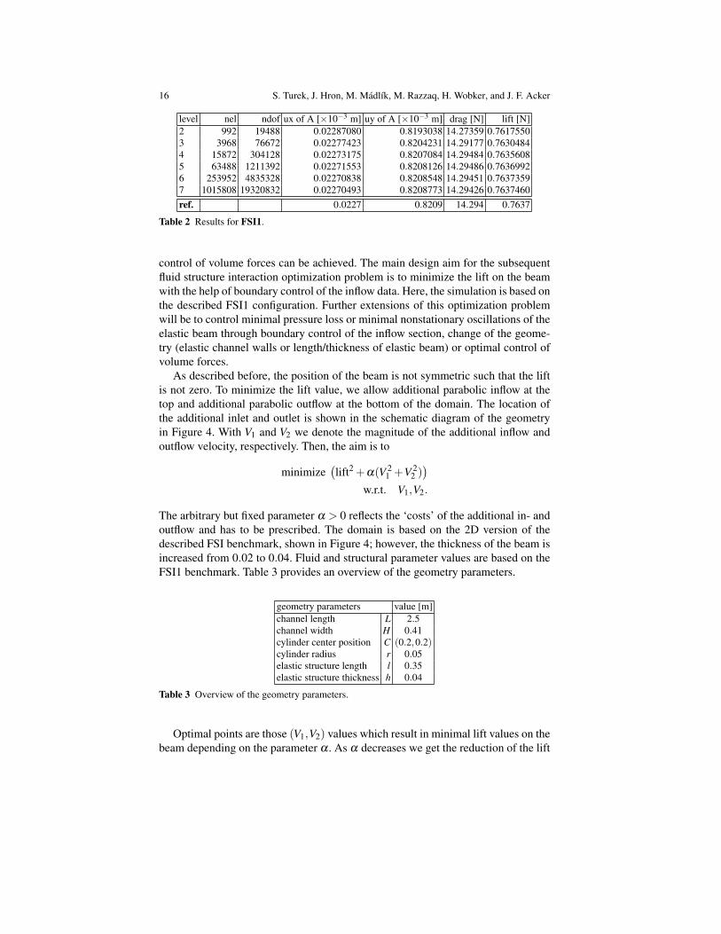
level nel ndof ux of A [×10−3 m] uy of A [×10−3 m] drag [N] lift [N]2 992 19488 0.02287080 0.8193038 14.27359 0.76175503 3968 76672 0.02277423 0.8204231 14.29177 0.76304844 15872 304128 0.02273175 0.8207084 14.29484 0.76356085 63488 1211392 0.02271553 0.8208126 14.29486 0.76369926 253952 4835328 0.02270838 0.8208548 14.29451 0.76373597 1015808 19320832 0.02270493 0.8208773 14.29426 0.7637460ref. 0.0227 0.8209 14.294 0.7637
Table 2 Results for FSI1.
control of volume forces can be achieved. The main design aim for the subsequentfluid structure interaction optimization problem is to minimize the lift on the beamwith the help of boundary control of the inflow data. Here, the simulation is based onthe described FSI1 configuration. Further extensions of this optimization problemwill be to control minimal pressure loss or minimal nonstationary oscillations of theelastic beam through boundary control of the inflow section, change of the geome-try (elastic channel walls or length/thickness of elastic beam) or optimal control ofvolume forces.
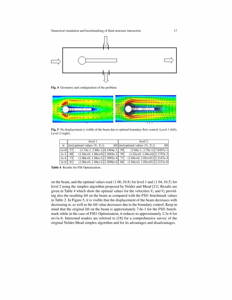
As described before, the position of the beam is not symmetric such that the liftis not zero. To minimize the lift value, we allow additional parabolic inflow at thetop and additional parabolic outflow at the bottom of the domain. The location ofthe additional inlet and outlet is shown in the schematic diagram of the geometryin Figure 4. With V1 and V2 we denote the magnitude of the additional inflow andoutflow velocity, respectively. Then, the aim is to
minimize(lift2 +α(V 2
1 +V 22 ))
w.r.t. V1,V2.
The arbitrary but fixed parameter α > 0 reflects the ‘costs’ of the additional in- andoutflow and has to be prescribed. The domain is based on the 2D version of thedescribed FSI benchmark, shown in Figure 4; however, the thickness of the beam isincreased from 0.02 to 0.04. Fluid and structural parameter values are based on theFSI1 benchmark. Table 3 provides an overview of the geometry parameters.
geometry parameters value [m]channel length L 2.5channel width H 0.41cylinder center position C (0.2,0.2)cylinder radius r 0.05elastic structure length l 0.35elastic structure thickness h 0.04
Table 3 Overview of the geometry parameters.
Optimal points are those (V1,V2) values which result in minimal lift values on thebeam depending on the parameter α . As α decreases we get the reduction of the lift
Numerical simulation and benchmarking of fluid-structure interaction 17
Fig. 4 Geometry and configuration of the problem.
Fig. 5 No displacement is visible of the beam due to optimal boundary flow control: Level 1 (left),Level 2 (right).
level 1 level 2α iter optimal values (V1,V2) lift iter optimal values (V1,V2) lift
1e+0 57 (3.74e-1, 3.88e-1) 8.1904e-1 59 (3.66e-1, 3.79e-1) 7.8497e-11e-2 60 (1.04e+0, 1.06e+0) 2.2684e-2 59 (1.02e+0, 1.04e+0) 2.1755e-21e-4 73 (1.06e+0, 1.08e+1) 2.3092e-4 71 (1.04e+0, 1.05e+01) 2.2147e-41e-6 81 (1.06e+0, 1.08e+1) 2.3096e-6 86 (1.04e+0, 1.05e+01) 2.2151e-6
Table 4 Results for FSI-Optimization.
on the beam, and the optimal values read (1.06,10.8) for level 1 and (1.04,10.5) forlevel 2 using the simplex algorithm proposed by Nelder and Mead [21]. Results aregiven in Table 4 which show the optimal values for the velocities V1 and V2 provid-ing also the resulting lift on the beam as compared with the FSI1 benchmark valuesin Table 2. In Figure 5, it is visible that the displacement of the beam decreases withdecreasing α , as well as the lift value decreases due to the boundary control. Keep inmind that the original lift on the beam is approximately 7.6e-1 for the FSI1 bench-mark while in the case of FSI1-Optimization, it reduces to approximately 2.3e-6 forα=1e-6. Interested readers are referred to [18] for a comprehensive survey of theoriginal Nelder-Mead simplex algorithm and for its advantages and disadvantages.
18 S. Turek, J. Hron, M. Madlık, M. Razzaq, H. Wobker, and J. F. Acker
6 Applications to hemodynamics
In the following, we consider the numerical simulation of special problems encoun-tered in the area of cardiovascular hemodynamics, namely flow interaction withthick-walled deformable material (here: the arterial walls) and rigid parts (here:stents), which can become a useful tool for deeper understanding of the onsetof diseases of the human circulatory system, as for example blood cell and inti-mal damages in stenosis, aneurysm rupture, evaluation of new surgery techniquesof the heart, arteries and veins (see [2, 19, 34] and the literature cited therein).In this contribution, prototypical studies are performed for brain aneurysms. Theword ‘aneurysm’ comes from the latin word aneurysma which means dilatation.An aneurysm is a local dilatation in the wall of a blood vessel, usually an artery,due to a defect, disease or injury. Typically, as the aneurysm enlarges, the arterialwall becomes thinner and eventually leaks or ruptures, causing subarachnoid hem-orrhage (SAH) (bleeding into brain fluid) or formation of a blood clot within thebrain. In the case of a vessel rupture, there is a hemorrhage, which is particularlyrapid and intense in case of an artery. In arteries the wall thickness can be up to 30%of the diameter and its local thickening can lead to the creation of an aneurysm. Theaim of numerical simulations is to relate the aneurysm state (unrupture or rupture)with wall pressure, wall deformation and effective wall stress. Such a relationshipwould provide information for the diagnosis and treatment of unruptured and rup-tured aneurysms by elucidating the risk of bleeding or rebleeding, respectively.
GiD
xy
z
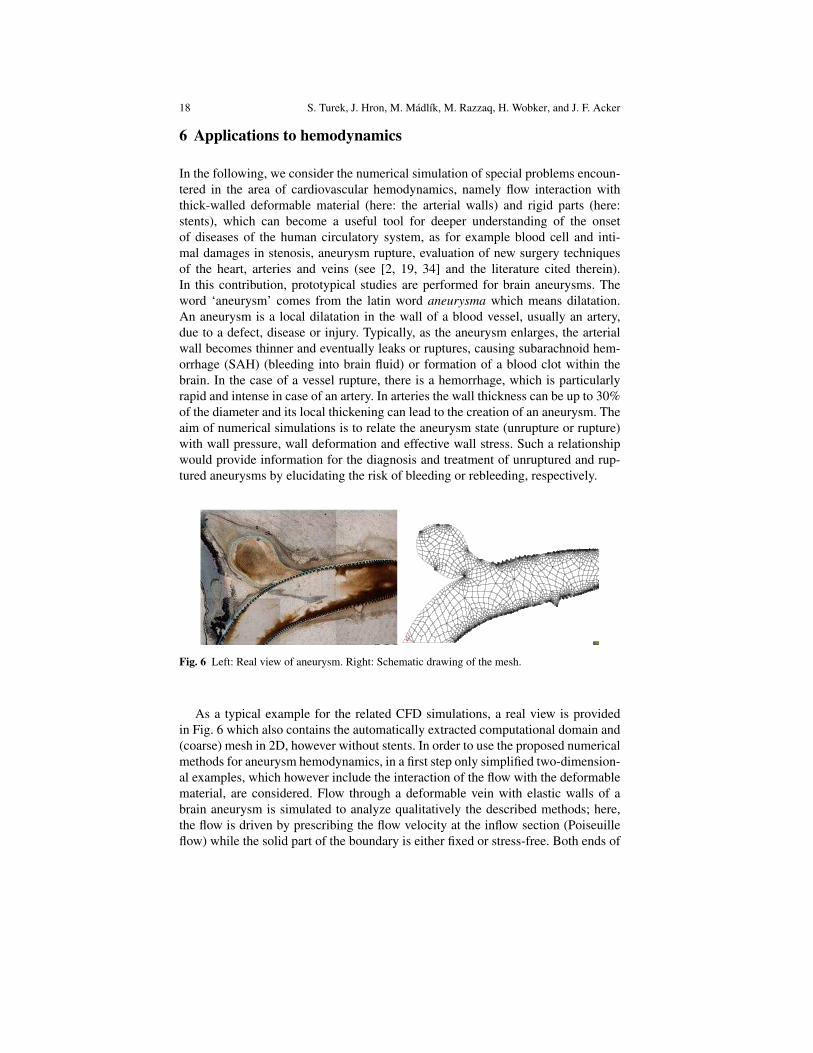
Fig. 6 Left: Real view of aneurysm. Right: Schematic drawing of the mesh.
As a typical example for the related CFD simulations, a real view is providedin Fig. 6 which also contains the automatically extracted computational domain and(coarse) mesh in 2D, however without stents. In order to use the proposed numericalmethods for aneurysm hemodynamics, in a first step only simplified two-dimension-al examples, which however include the interaction of the flow with the deformablematerial, are considered. Flow through a deformable vein with elastic walls of abrain aneurysm is simulated to analyze qualitatively the described methods; here,the flow is driven by prescribing the flow velocity at the inflow section (Poiseuilleflow) while the solid part of the boundary is either fixed or stress-free. Both ends of
Numerical simulation and benchmarking of fluid-structure interaction 19
the walls are fixed, and the flow is driven by a periodical change of the inflow at theright end.
6.1 Geometry of the problem
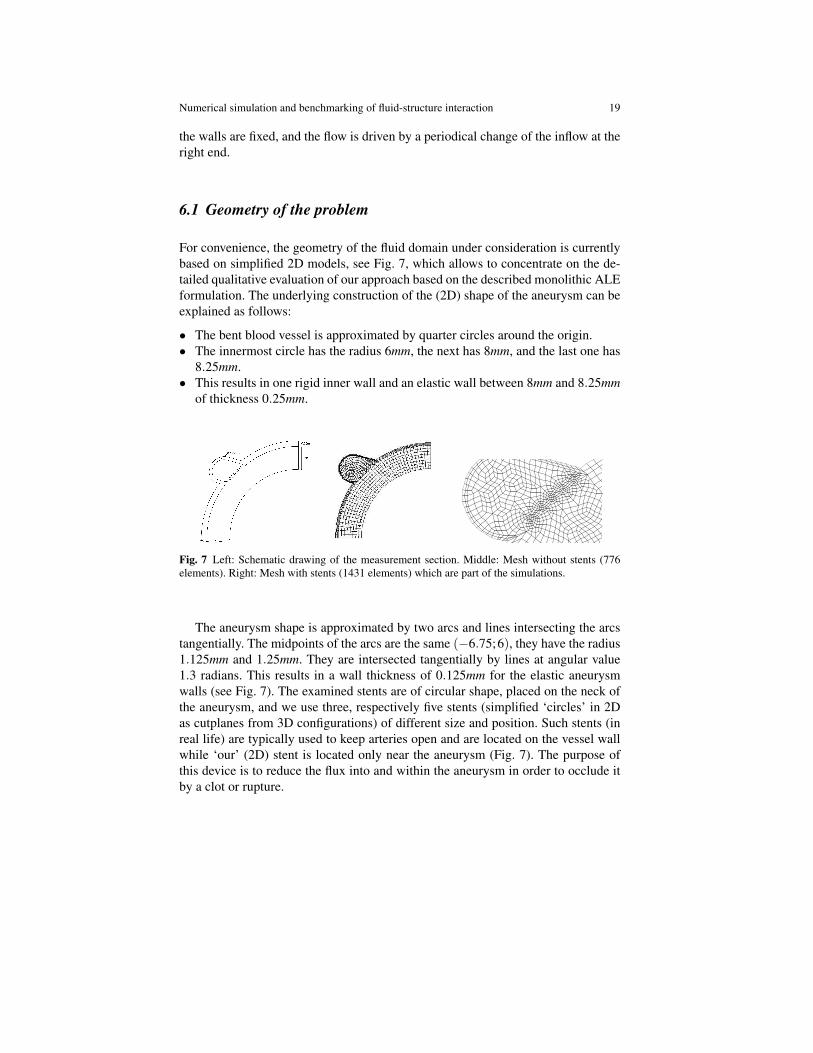
For convenience, the geometry of the fluid domain under consideration is currentlybased on simplified 2D models, see Fig. 7, which allows to concentrate on the de-tailed qualitative evaluation of our approach based on the described monolithic ALEformulation. The underlying construction of the (2D) shape of the aneurysm can beexplained as follows:
• The bent blood vessel is approximated by quarter circles around the origin.• The innermost circle has the radius 6mm, the next has 8mm, and the last one has
8.25mm.• This results in one rigid inner wall and an elastic wall between 8mm and 8.25mm
of thickness 0.25mm.
Fig. 7 Left: Schematic drawing of the measurement section. Middle: Mesh without stents (776elements). Right: Mesh with stents (1431 elements) which are part of the simulations.
The aneurysm shape is approximated by two arcs and lines intersecting the arcstangentially. The midpoints of the arcs are the same (−6.75;6), they have the radius1.125mm and 1.25mm. They are intersected tangentially by lines at angular value1.3 radians. This results in a wall thickness of 0.125mm for the elastic aneurysmwalls (see Fig. 7). The examined stents are of circular shape, placed on the neck ofthe aneurysm, and we use three, respectively five stents (simplified ‘circles’ in 2Das cutplanes from 3D configurations) of different size and position. Such stents (inreal life) are typically used to keep arteries open and are located on the vessel wallwhile ‘our’ (2D) stent is located only near the aneurysm (Fig. 7). The purpose ofthis device is to reduce the flux into and within the aneurysm in order to occlude itby a clot or rupture.
20 S. Turek, J. Hron, M. Madlık, M. Razzaq, H. Wobker, and J. F. Acker
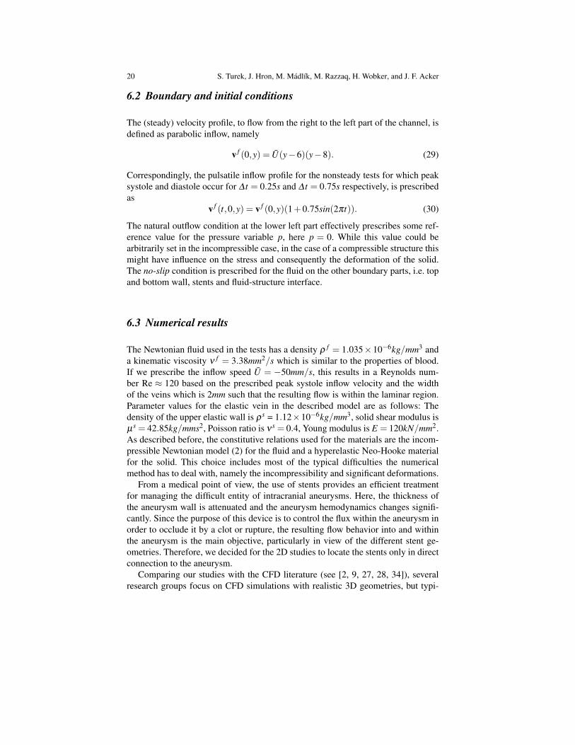
6.2 Boundary and initial conditions
The (steady) velocity profile, to flow from the right to the left part of the channel, isdefined as parabolic inflow, namely
v f (0,y) = U(y−6)(y−8). (29)
Correspondingly, the pulsatile inflow profile for the nonsteady tests for which peaksystole and diastole occur for ∆ t = 0.25s and ∆ t = 0.75s respectively, is prescribedas
v f (t,0,y) = v f (0,y)(1+0.75sin(2πt)). (30)
The natural outflow condition at the lower left part effectively prescribes some ref-erence value for the pressure variable p, here p = 0. While this value could bearbitrarily set in the incompressible case, in the case of a compressible structure thismight have influence on the stress and consequently the deformation of the solid.The no-slip condition is prescribed for the fluid on the other boundary parts, i.e. topand bottom wall, stents and fluid-structure interface.
6.3 Numerical results
The Newtonian fluid used in the tests has a density ρ f = 1.035×10⁻⁶kg/mm3 anda kinematic viscosity ν f = 3.38mm2/s which is similar to the properties of blood.If we prescribe the inflow speed U = −50mm/s, this results in a Reynolds num-ber Re ≈ 120 based on the prescribed peak systole inflow velocity and the widthof the veins which is 2mm such that the resulting flow is within the laminar region.Parameter values for the elastic vein in the described model are as follows: Thedensity of the upper elastic wall is ρs = 1.12×10⁻⁶kg/mm3, solid shear modulus isµs = 42.85kg/mms2, Poisson ratio is νs = 0.4, Young modulus is E = 120kN/mm2.As described before, the constitutive relations used for the materials are the incom-pressible Newtonian model (2) for the fluid and a hyperelastic Neo-Hooke materialfor the solid. This choice includes most of the typical difficulties the numericalmethod has to deal with, namely the incompressibility and significant deformations.
From a medical point of view, the use of stents provides an efficient treatmentfor managing the difficult entity of intracranial aneurysms. Here, the thickness ofthe aneurysm wall is attenuated and the aneurysm hemodynamics changes signifi-cantly. Since the purpose of this device is to control the flux within the aneurysm inorder to occlude it by a clot or rupture, the resulting flow behavior into and withinthe aneurysm is the main objective, particularly in view of the different stent ge-ometries. Therefore, we decided for the 2D studies to locate the stents only in directconnection to the aneurysm.
Comparing our studies with the CFD literature (see [2, 9, 27, 28, 34]), severalresearch groups focus on CFD simulations with realistic 3D geometries, but typi-
Numerical simulation and benchmarking of fluid-structure interaction 21
cally assuming rigid walls. In contrast, we concentrate on the complex interactionbetween elastic deformations and flow perturbations induced by the stents. At themoment, we are only able to perform these simulations in 2D. However, with thesestudies we should be able to analyze qualitatively the influence of geometrical de-tails onto the elastic material behavior, particularly in view of more complex bloodmodels and constitutive equations for the structure. Therefore, the aims of our cur-rent studies can be described as follows:
1. What is the influence of the elasticity of the walls onto the flow behavior insidethe aneurysm, particularly w.r.t. the resulting shape of the aneurysm?
2. What is the influence of the geometrical details of the (2D) stents, that meansshape, size, position, on the flow into and inside the aneurysm?
3. Do both aspects, small-scale geometrical details as well as elastic fluid-structureinteraction, have to be considered simultaneously or is one of them negligible infirst order approximation?
4. Are modern numerical methods and corresponding CFD simulation tools able tosimulate qualitatively the multiphysics behavior of such biomedical configura-tions?
In the following, we show some corresponding results for the described prototypicalaneurysm geometry, first for the steady state inflow profile, followed by nonsteadytests for the pulsatile inflow, both with rigid and elastic walls, respectively.
6.3.1 Steady configurations
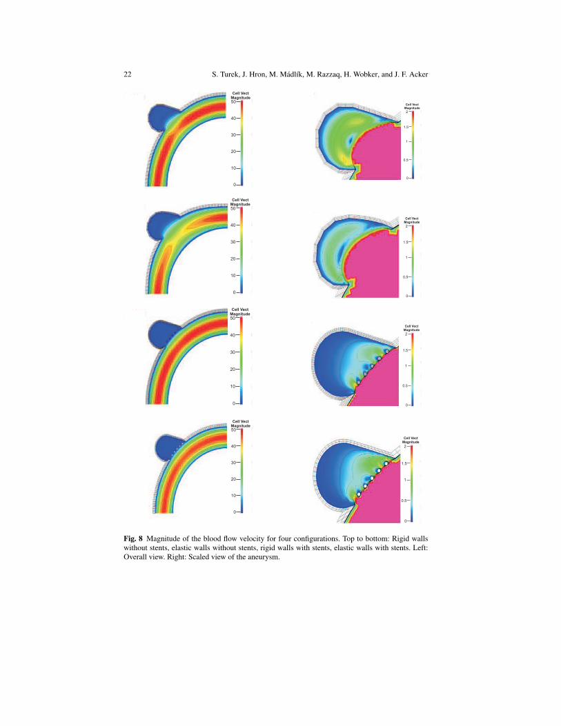
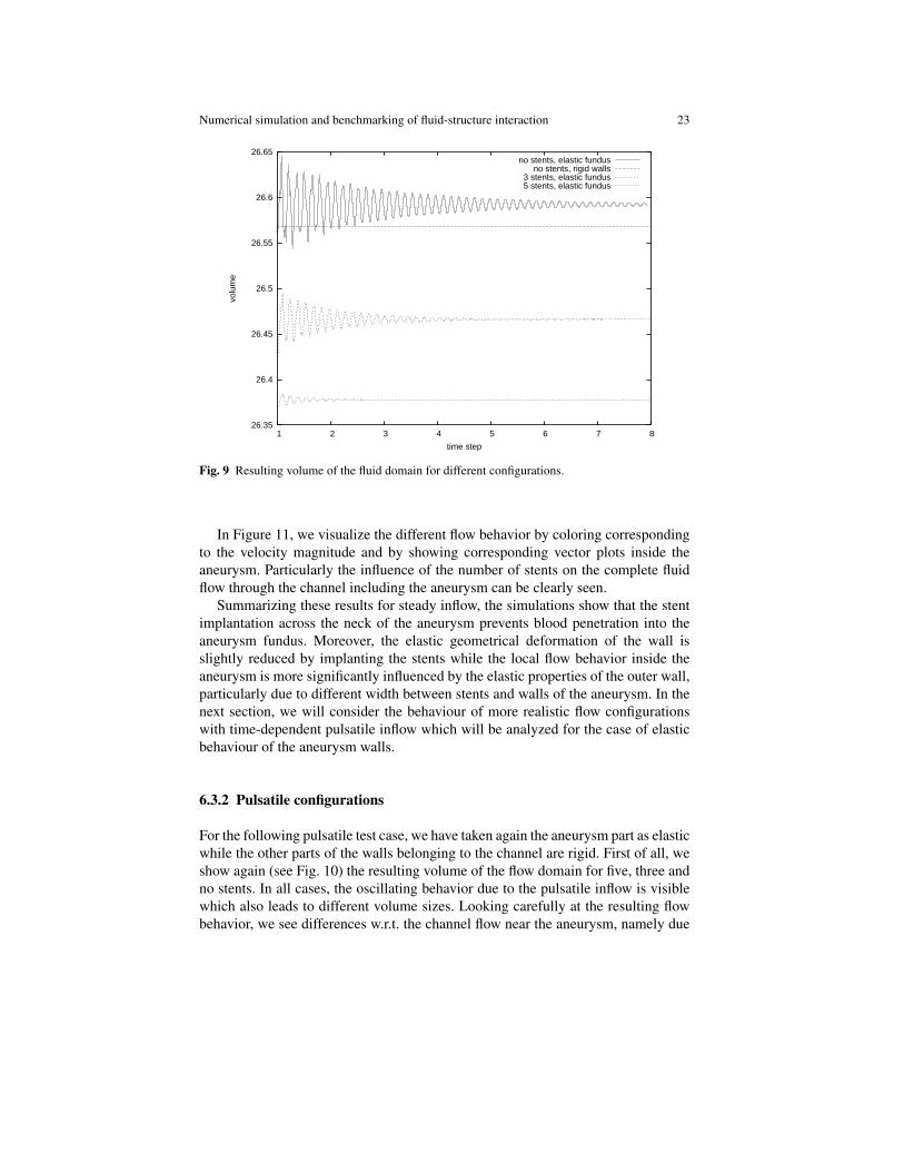
Due to the given inflow profile, which is not time-dependent, and due to the lowReynolds numbers, the flow behavior leads to a steady state which only depends onthe elasticity and the shape of the stents. Moreover, for the following simulations,we only treat the aneurysm wall as elastic structure. Then, the aneurysm undergoessome slight deformations which can hardly be seen in the following figures. How-ever, they result in a different volume of the flow domain (see Fig. 9) and lead toa significantly different local flow behavior since the spacing between stents andelastic walls may change (see Figure 8).
22 S. Turek, J. Hron, M. Madlık, M. Razzaq, H. Wobker, and J. F. Acker
Cell VectMagnitude
0
10
20
30
40
50Cell Vect
Magnitude
0
0.5
1
1.5
2
Cell VectMagnitude
0
10
20
30
40
50
Cell VectMagnitude
0
0.5
1
1.5
2
Cell VectMagnitude
0
10
20
30
40
50
Cell VectMagnitude
0
0.5
1
1.5
2
Cell VectMagnitude
0
10
20
30
40
50
Cell VectMagnitude
0
0.5
1
1.5
2
Fig. 8 Magnitude of the blood flow velocity for four configurations. Top to bottom: Rigid wallswithout stents, elastic walls without stents, rigid walls with stents, elastic walls with stents. Left:Overall view. Right: Scaled view of the aneurysm.
Numerical simulation and benchmarking of fluid-structure interaction 23
26.35
26.4
26.45
26.5
26.55
26.6
26.65
1 2 3 4 5 6 7 8
volu
me
time step
no stents, elastic fundusno stents, rigid walls
3 stents, elastic fundus5 stents, elastic fundus
Fig. 9 Resulting volume of the fluid domain for different configurations.
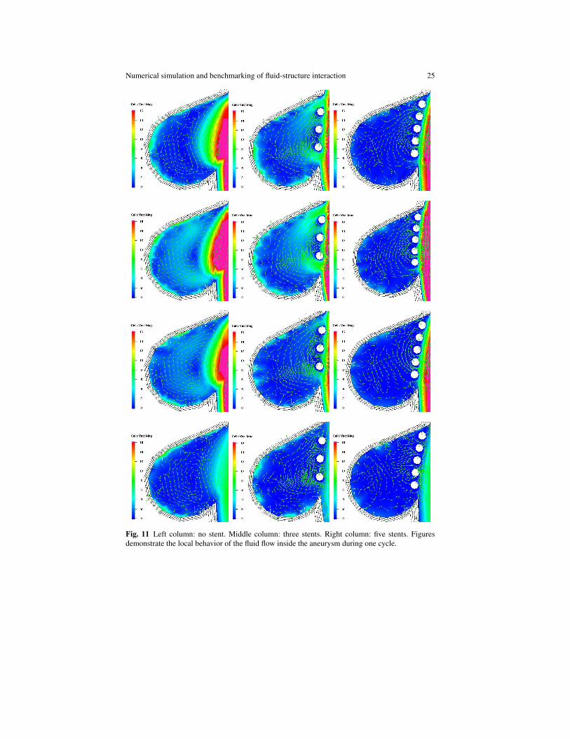
In Figure 11, we visualize the different flow behavior by coloring correspondingto the velocity magnitude and by showing corresponding vector plots inside theaneurysm. Particularly the influence of the number of stents on the complete fluidflow through the channel including the aneurysm can be clearly seen.
Summarizing these results for steady inflow, the simulations show that the stentimplantation across the neck of the aneurysm prevents blood penetration into theaneurysm fundus. Moreover, the elastic geometrical deformation of the wall isslightly reduced by implanting the stents while the local flow behavior inside theaneurysm is more significantly influenced by the elastic properties of the outer wall,particularly due to different width between stents and walls of the aneurysm. In thenext section, we will consider the behaviour of more realistic flow configurationswith time-dependent pulsatile inflow which will be analyzed for the case of elasticbehaviour of the aneurysm walls.
6.3.2 Pulsatile configurations
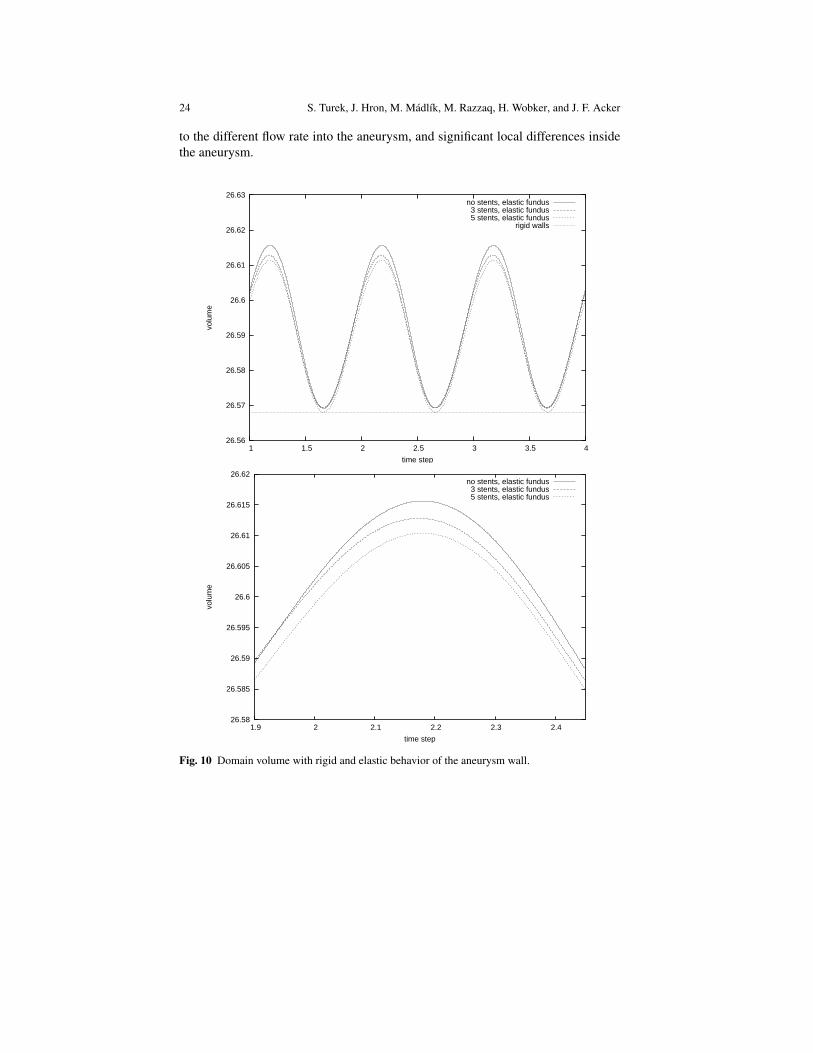
For the following pulsatile test case, we have taken again the aneurysm part as elasticwhile the other parts of the walls belonging to the channel are rigid. First of all, weshow again (see Fig. 10) the resulting volume of the flow domain for five, three andno stents. In all cases, the oscillating behavior due to the pulsatile inflow is visiblewhich also leads to different volume sizes. Looking carefully at the resulting flowbehavior, we see differences w.r.t. the channel flow near the aneurysm, namely due
24 S. Turek, J. Hron, M. Madlık, M. Razzaq, H. Wobker, and J. F. Acker
to the different flow rate into the aneurysm, and significant local differences insidethe aneurysm.
26.56
26.57
26.58
26.59
26.6
26.61
26.62
26.63
1 1.5 2 2.5 3 3.5 4
volu
me
time step
no stents, elastic fundus3 stents, elastic fundus5 stents, elastic fundus
rigid walls
26.58
26.585
26.59
26.595
26.6
26.605
26.61
26.615
26.62
1.9 2 2.1 2.2 2.3 2.4
volu
me
time step
no stents, elastic fundus3 stents, elastic fundus5 stents, elastic fundus
Fig. 10 Domain volume with rigid and elastic behavior of the aneurysm wall.
Numerical simulation and benchmarking of fluid-structure interaction 25
Fig. 11 Left column: no stent. Middle column: three stents. Right column: five stents. Figuresdemonstrate the local behavior of the fluid flow inside the aneurysm during one cycle.
26 S. Turek, J. Hron, M. Madlık, M. Razzaq, H. Wobker, and J. F. Acker
6.3.3 Extension to 3D
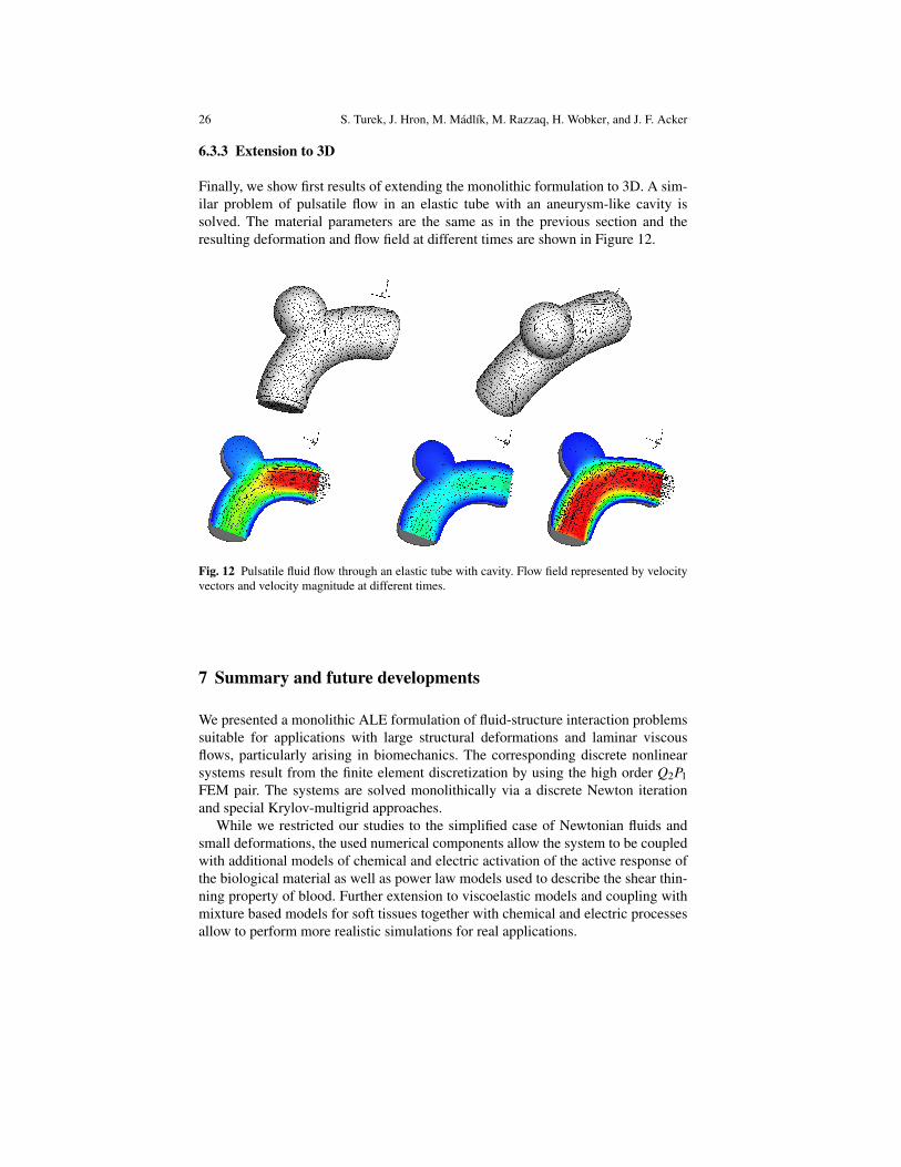
Finally, we show first results of extending the monolithic formulation to 3D. A sim-ilar problem of pulsatile flow in an elastic tube with an aneurysm-like cavity issolved. The material parameters are the same as in the previous section and theresulting deformation and flow field at different times are shown in Figure 12.
Fig. 12 Pulsatile fluid flow through an elastic tube with cavity. Flow field represented by velocityvectors and velocity magnitude at different times.
7 Summary and future developments
We presented a monolithic ALE formulation of fluid-structure interaction problemssuitable for applications with large structural deformations and laminar viscousflows, particularly arising in biomechanics. The corresponding discrete nonlinearsystems result from the finite element discretization by using the high order Q2P1FEM pair. The systems are solved monolithically via a discrete Newton iterationand special Krylov-multigrid approaches.
While we restricted our studies to the simplified case of Newtonian fluids andsmall deformations, the used numerical components allow the system to be coupledwith additional models of chemical and electric activation of the active response ofthe biological material as well as power law models used to describe the shear thin-ning property of blood. Further extension to viscoelastic models and coupling withmixture based models for soft tissues together with chemical and electric processesallow to perform more realistic simulations for real applications.
Numerical simulation and benchmarking of fluid-structure interaction 27
We applied the presented numerical techniques to FSI benchmarking settings(‘channel flow around cylinder with attached elastic beam’, see [30]) which allowthe validation and also evaluation of different numerical solution approaches forfluid-structure interaction problems. Moreover, we examined prototypically the in-fluence of endovascular stent implantation on aneurysm hemodynamics. The aimwas, first of all, to study the influence of the elasticity of the walls on the flow be-havior inside the aneurysm. Moreover, different geometrical configurations of im-planted stent structures have been analyzed in 2D. These 2D results are far from pro-viding quantitative results for such a complex multiphysics configuration, but theyallow a qualitative analysis w.r.t. both considered components, namely the elasticbehavior of the structural parts and the multiscale flow behavior due to the geo-metrical details of the stents. We believe that such basic studies are helpful for thedevelopment of future ‘Virtual Flow Laboratories’ which individually assist to de-sign personal medical tools.
Acknowledegment:The authors want to express their gratitude to the German Research Association(DFG), funding the project as part of FOR493 and TRR30, the Jindrich NecasCenter for Mathematical Modeling, project LC06052 financed by MSMT, and theHigher Education Commission (HEC) of Pakistan for their financial support of thestudy. The present material is also based upon work kindly supported by the Hom-burger Forschungsforderungsprogramm (HOMFOR) 2008.
References
[1] P. R. Amestoy, I. S. Duff, and J. Y. L’Excellent. Multifrontal parallel dis-tributed symmetric and unsymmetric solvers. Computer Methods in AppliedMechanics and Engineering, 184(2-4):501 – 520, 2000.
[2] S. Appanaboyina, F. Mut, R. Lohner, E. Scrivano, C. Miranda, P. Lylyk, C. Put-man, and J. Cebral. Computational modelling of blood flow in side arterialbranches after stenting of cerebral aneurysm. International Journal of Com-putational Fluid Dynamics, 22:669–676, 2008.
[3] D. N. Arnold, D. Boffi, and R. S. Falk. Approximation by quadrilateral finiteelement. Math. Comput., 71:909–922, 2002.
[4] R. Barrett, M. Berry, T. F. Chan, J. Demmel, J. Donato, J. Dongarra, V. Ei-jkhout, R. Pozo, C. Romine, and H. Van der Vorst. Templates for the solutionof linear systems: Building blocks for iterative methods. SIAM, Philadelphia,PA, second edition, 1994.
[5] D. Boffi and L.. Gastaldi. On the quadrilateral Q2P1 element for the Stokesproblem. Int. J. Numer. Meth. Fluids., 39:1001–1011, 2002.
[6] R. Bramley and X. Wang. SPLIB: A library of iterative methods for sparselinear systems. Department of Computer Science, Indiana University, Bloom-
28 S. Turek, J. Hron, M. Madlık, M. Razzaq, H. Wobker, and J. F. Acker
ington, IN, 1997. http://www.cs.indiana.edu/ftp/bramley/splib.tar.gz.
[7] H. Damanik, J. Hron, A. Ouazzi, and S. Turek. A monolithic FEM approachfor non-isothermal incompressible viscous flows. Journal of ComputationalPhysics, 228:3869–3881, 2009.
[8] T. A. Davis and I. S. Duff. A combined unifrontal/multifrontal method forunsymmetric sparse matrices. ACM Trans. Math. Software, 25(1):1–19, 1999.
[9] M. A. Fernandez, J-F. Gerbeau, and V. Martin. Numerical simulation of bloodflows through a porous interface. ESAIM: Mathematical Modelling and Nu-merical Analysis, 42:961–990, 2008.
[10] M. Fortin. Old and new finite elements for incompressible flows. InternationalJournal for Numerical Methods in Fluids, 1(4), 1981.
[11] Y. C. Fung. Biomechanics: Mechanical Properties of Living Tissues. Springer-Verlag, New York, 1993.
[12] R. Glowinski. Finite element method for incompressible viscous flow. In P. GCiarlet and J. L. Lions, editors, Handbook of Numerical Analysis, Volume IX,,pages 3–1176. North-Holland, Amsterdam, 2003.
[13] P. M. Gresho. On the theory of semi-implicit projection methods for viscousincompressible flow and its implementation via a finite element method thatalso introduces a nearly consistent mass matrix, part 1: Theory. Int. J. Numer.Meth. Fluids., 11:587–620, 1990.
[14] G. A. Holzapfel. A continuum approach for engineering. John Wiley andSons, Chichester, UK, 2000.
[15] G. A. Holzapfel. Determination of meterial models for arterial walls fromuni-axial extension tests and histological structure. International Journal forNumerical Methods in Fluids, 238(2):290–302, 2006.
[16] J. Hron, A. Ouazzi, and S. Turek. A computational comparison of two FEMsolvers for nonlinear incompressible flow. In E. Bansch, editor, Challenges inScientific Computing, LNCSE:53, pages 87–109. Springer, 2002.
[17] J. Hron and S. Turek. A monolithic FEM/multigrid solver for ALE formu-lation of fluid structure interaction with application in biomechanics. In H.-J. Bungartz and M. Schafer, editors, Fluid-Structure Interaction: Modelling,Simulation, Optimisation, LNCSE:53. Springer, 2006.
[18] J. C. Lagarias, J. A. Reeds, M. H. Wright, and P. E. Wright. Convergenceproperties of the Nelder-Mead simplex method in low dimensions. SIAM J.Optim., 9:112–147, 1998.
[19] R. Lohner, J. Cebral, and S. Appanaboyina. Parabolic recovery of boundarygradients. Communications in Numerical Methods in Engineering, 24:1611–1615, 2008.
[20] D. A. McDonald. Blood flow in arteries. In second ed. Edward Arnold, 1974.[21] J. A. Nelder and R. Mead. A simplex method for function minimization. Com-
puter Journal, 7(4):308–313, 1965.[22] R. Rannacher and S. Turek. A simple nonconforming quadrilateral Stokes
element. Numer. Methods Partial Differential Equations., 8:97–111, 1992.
Numerical simulation and benchmarking of fluid-structure interaction 29
[23] M. Razzaq. Numerical techniques for solving fluid-structure interaction prob-lems with applications to bio-engineering. PhD Thesis, TU Dortmund, to ap-pear, 2010.
[24] M. Razzaq, J. Hron, and S. Turek. Numerical simulation of laminar incom-pressible fluid-structure interaction for elastic material with point constraints.In R. Rannacher and A. Sequeira, editors, Advances in Mathematical FluidMechancis-Dedicated to Giovanni paolo Galdi on the Occasion of his 60thBirthday. Springer, in print, 2009.
[25] T. E. Tezduyar, S. Sathe, T. Cragin, B. Nanna, B.S. Conklin, J. Pausewang,and M. Schwaab. Modeling of fluid structure interactions with the space timefinite elements: Arterial fluid mechanics. International Journal for NumericalMethods in Fluids, 54:901–922, 2007.
[26] T. E. Tezduyar, S. Sathe, M. Schwaab, and B.S. Conklin. Arterial fluid me-chanics modeling with the stabilized space time fluid structure interaction tech-nique. International Journal for Numerical Methods in Fluids, 57:601–629,2008.
[27] R. Torri, M. Oshima, T. Kobayashi, K. Takagi, and T.E. Tezduyar. Influence ofwall elasticity in patient-specific hemodynamic simulations. Computers andFluids, 36:160–168, 2007.
[28] R. Torri, M. Oshima, T. Kobayashi, K. Takagi, and T.E. Tezduyar. Numericalinvestigation of the effect of hypertensive blood pressure on cerebral aneurysmdependence of the effect on the aneurysm shape. International Journal forNumerical Methods in Fluids, 54:995–1009, 2007.
[29] S. Turek. Efficient Solvers for Incompressible Flow Problems: An Algorithmicand Computational Approach. Springer-Verlag, 1999.
[30] S. Turek and J. Hron. Proposal for numerical benchmarking of fluid-structureinteraction between an elastic object and laminar incompressible flow. In H.-J. Bungartz and M. Schafer, editors, Fluid-Structure Interaction: Modelling,Simulation, Optimisation, LNCSE:53. Springer, 2006.
[31] S. Turek, L. Rivkind, J. Hron, and R. Glowinski. Numerical study of a modi-fied time-steeping theta-scheme for incompressible flow simulations. Journalof Scientific Computing, 28:533–547, 2006.
[32] S. Turek and M. Schafer. Benchmark computations of laminar flow aroundcylinder. In E.H. Hirschel, editor, Flow Simulation with High-PerformanceComputers II, volume 52 of Notes on Numerical Fluid Mechanics. Vieweg,1996. co. F. Durst, E. Krause, R. Rannacher.
[33] S. Turek and R. Schmachtel. Fully coupled and operator-splitting approachesfor natural convection flows in enclosures. International Journal for Numeri-cal Methods in Fluids, 40:1109–1119, 2002.
[34] A. Valencia, D. Ladermann, R. Rivera, E. Bravo, and M. Galvez. Bloodflow dynamics and fluid–structure interaction in patient-specific bifurcatingcerebral aneurysms. International Journal for Numerical Methods in Fluids,58:1081–1100, 2008.
[35] S. P. Vanka. Implicit multigrid solutions of Navier-Stokes equations in primi-tive variables. J. of Comp. Phys., 65:138–158, 1985.