1

Abstract The numerical simulation of a large excavation (145 m x 165 m) for the construction of a watch production centre is described in this paper. A three dimensional non-linear coupled finite element analysis has been conducted with Z_Soil 3D v5 [1] in order to verify and optimise the designed retaining system as well as to carefully predict the settlements, as many manufactures stand in the surrounds. Keywords: 3D case study, finite elements, coupled analysis,

retaining system optimisation, modelling-measurement comparison 1 Introduction In the neighbourhood of Geneva, the construction of a watch production centre has been planned. The project involves the execution of a large excavation in soft and saturated clays. It concerns a 145 x 165 m soil surface with a maximum excavation level of about – 20 m. The designed retaining system is composed of a slurry wall braced at its top. The bracing leans on a 130 m diameter circular reinforced concrete beam supported by piles linked with a buried circular internal slurry wall located at the excavation’s bottom (see Figure 1).

A 3D numerical simulation has been conducted with Z_Soil 3D v5 [1] in order to control and optimise all the components interacting in the project. A similar case (large dimensions, similar soil conditions and retaining system) constructed in the 1970’s has been used as a real-scale test in order to precise the soil parameters and the hydro-mechanical behaviour with the help of a back analysis.

In section 2, the different modelling assumptions are described. This includes

hydrogeotechnical conditions and finite element model characteristics. The main results of the study are then summarised in section 3. A reference case is described

Numerical Simulation of Earthworks and Retaining System for a Large Excavation

F. Geiser*+, S. Commend*+ and J.Crisinel*

* De Cerenville Geotechnique SA, Ecublens, Switzerland + now at : ComSA Ingenieurs Conseils SA, Renens, Switzerland

2

in details, followed by a parametric study. Finally, as the project is currently under construction, a brief comparison between in situ observations and numerical predictions is given in the conclusion.

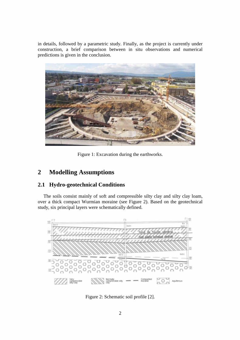
Figure 1: Excavation during the earthworks.

2 Modelling Assumptions 2.1 Hydro-geotechnical Conditions

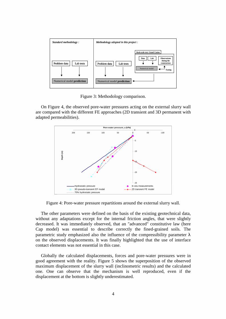
The soils consist mainly of soft and compressible silty clay and silty clay loam, over a thick compact Wurmian moraine (see Figure 2). Based on the geotechnical study, six principal layers were schematically defined.

Figure 2: Schematic soil profile [2].

3

Only the first five layers - belonging to glacier retreat deposits - are modelled, as the moraine is assumed to be stiff enough in comparison to the other soils. Thus fixed boundary conditions are set at –39.7 m depth. The mechanical soil behaviour is modelled with a Cap model for the silty clays and with a Drucker-Prager yield surface for the first sandy layer.

The soil properties are shown in Table 1. They were defined on the basis of

laboratory tests and a real-scale test in the neighbourhood (see § 2.2).

Description Depth [m]

E [MPa]

ν

[-] c'

[kPa]φ' [°]

ψ

[°]

γ

[kN/m3] e0 [-]

kx = kz [m/s]

ky [m/s]

λ

[-]

pc0 [kPa]

R [-]

Sand and sandy silt

0.5 to -3.05 80 0.38 2 27 10 20.9 0.50 1E-06 1E-06 - - -

Silty clay loam and silty clay

- 3.05 to - 8.0 60 0.38 5 22 7 21.0 0.73 1E-03 1E-03 0.15 110 1.8

Silty clay - 8.0 to - 21.75 45 0.38 4 21 7 21.0 0.99 8E-06 8E-06 0.15 165-

250 1.8

Silty clay -21.75 to -28.8 55 0.38 6 21 7 21.0 0.82 8E-06 6E-06 0.10 330 1.8

Silty clay loam

-28.8 to -39.7 70 0.38 6 23 8 21.0 0.66 8E-06 8E-06 0.10 450 1.8

Table 1: Soil properties.

A saturation level is measured at -2.45 depth and is modelled as a groundwater

table. Further details on the modelling of the transient aspect of the problem are given in § 2.2. 2.2 "Grand Casino": Back-analysis on a Similar Case As shown schematically in Figure 3, one of the key points of this numerical simulation was to receive data from a similar project in the same glacier retreat deposit soils in Geneva, namely the "Grand Casino" project. Unlike most numerical approaches, it was consequently possible to test and verify the importance of the different parameters on a real-scale case, as numerous field measurements were available. More details are given on this project in [3], [4] and [5].

The change in the pore-water pressure was observed to be the main factor influencing the general behaviour in this project. As the soil permeabilities are low, the hydraulic conditions remain transient during the construction. For a year long excavation, the pore-water pressure looses about 25 to 30 % of its initial value. After reproducing these time-effects on a 2D model, a "pseudo-transient" model was developed for the 3D approach, in order to avoid days-long calculations with a time dependent problem. The permeabilities of the soils were basically modified in order to obtain pore-water pressures similar to the observed ones, but with a permanent hydraulic approach.

4

Standard methodology :

Problem data Lab tests

Numerical model prediction

Methodology adopted in this project :

Problem data Lab tests

Numerical model prediction

Data Lab

Numerical model

Observations during the

construction

Tuning

Real-scale test: Grand Casino

Standard methodology :

Problem data Lab tests

Numerical model prediction

Methodology adopted in this project :

Problem data Lab tests

Numerical model prediction

Data Lab

Numerical model

Observations during the

construction

Tuning

Real-scale test: Grand Casino

Figure 3: Methodology comparison.

On Figure 4, the observed pore-water pressures acting on the external slurry wall are compared with the different FE approaches (2D transient and 3D permanent with adapted permeabilities).

-25

-20

-15

-10

-5

0-100-50050100150200

Pore-w ater pressure, u (kPa)

Dep

th (m

)

Hydrostatic pressure In situ measurements3D pseudo-transient EF model 2D transient FE model 70% hydrostatic pressure

Figure 4: Pore-water pressure repartitions around the external slurry wall.

The other parameters were defined on the basis of the existing geotechnical data,

without any adaptations except for the internal friction angles, that were slightly decreased. It was immediately observed, that an "advanced" constitutive law (here Cap model) was essential to describe correctly the fined-grained soils. The parametric study emphasized also the influence of the compressibility parameter λ on the observed displacements. It was finally highlighted that the use of interface contact elements was not essential in this case.

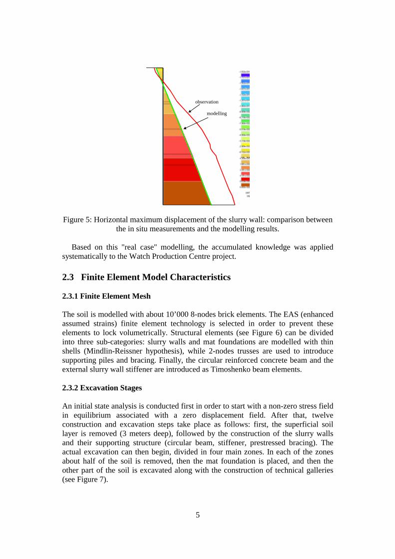
Globally the calculated displacements, forces and pore-water pressures were in

good agreement with the reality. Figure 5 shows the superposition of the observed maximum displacement of the slurry wall (inclinometric results) and the calculated one. One can observe that the mechanism is well reproduced, even if the displacement at the bottom is slightly underestimated.

5

observation

modelling

Figure 5: Horizontal maximum displacement of the slurry wall: comparison between the in situ measurements and the modelling results.

Based on this "real case" modelling, the accumulated knowledge was applied

systematically to the Watch Production Centre project.

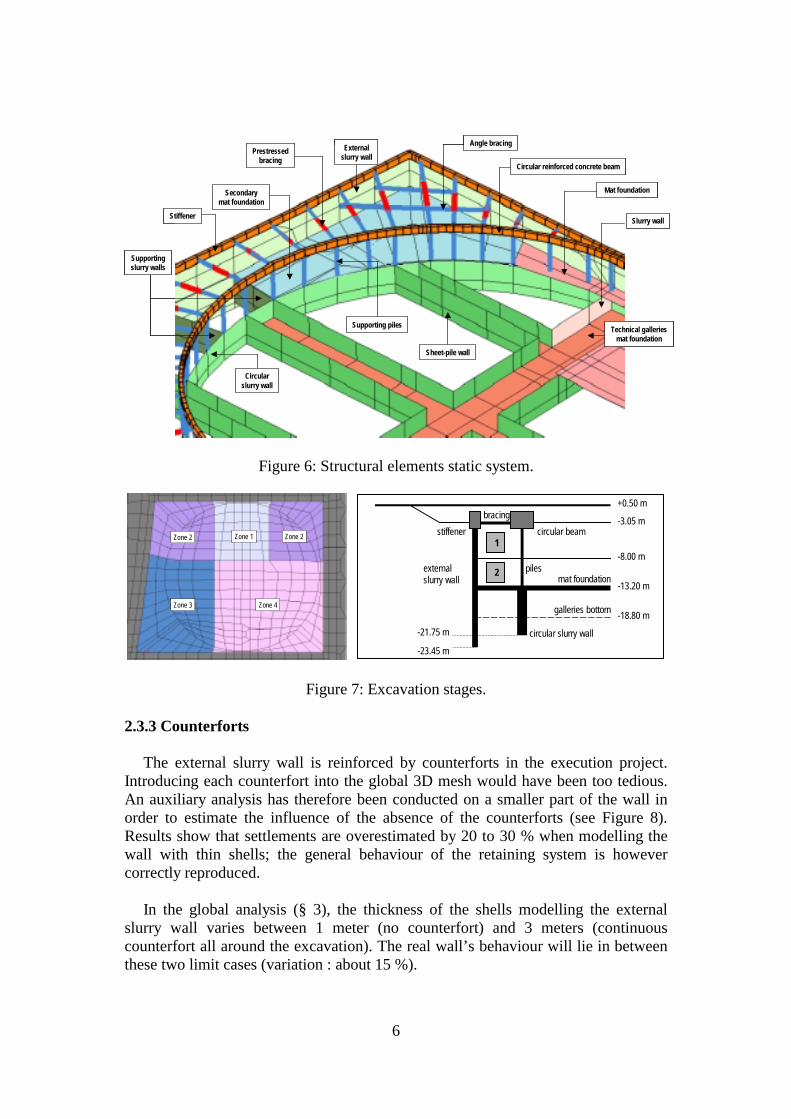
2.3 Finite Element Model Characteristics 2.3.1 Finite Element Mesh The soil is modelled with about 10’000 8-nodes brick elements. The EAS (enhanced assumed strains) finite element technology is selected in order to prevent these elements to lock volumetrically. Structural elements (see Figure 6) can be divided into three sub-categories: slurry walls and mat foundations are modelled with thin shells (Mindlin-Reissner hypothesis), while 2-nodes trusses are used to introduce supporting piles and bracing. Finally, the circular reinforced concrete beam and the external slurry wall stiffener are introduced as Timoshenko beam elements. 2.3.2 Excavation Stages An initial state analysis is conducted first in order to start with a non-zero stress field in equilibrium associated with a zero displacement field. After that, twelve construction and excavation steps take place as follows: first, the superficial soil layer is removed (3 meters deep), followed by the construction of the slurry walls and their supporting structure (circular beam, stiffener, prestressed bracing). The actual excavation can then begin, divided in four main zones. In each of the zones about half of the soil is removed, then the mat foundation is placed, and then the other part of the soil is excavated along with the construction of technical galleries (see Figure 7).

6

Stiffener

Supportingslurry walls

Secondarymat foundation

Prestressedbracing

Angle bracing

Circular reinforced concrete beam

Sheet-pile wall

Technical galleriesmat foundation

Slurry wall

Mat foundation

Externalslurry wall

Supporting piles

Circularslurry wall

Stiffener

Supportingslurry walls

Secondarymat foundation

Prestressedbracing

Angle bracing

Circular reinforced concrete beam

Sheet-pile wall

Technical galleriesmat foundation

Slurry wall

Mat foundation

Externalslurry wall

Supporting piles

Circularslurry wall

Figure 6: Structural elements static system.

+0.50 m

-3.05 m

-8.00 m

-13.20 m

-18.80 m

stiffener

externalslurry wall

circular slurry wall

circular beam

pilesmat foundation

galleries bottom

1

2

bracing

-21.75 m

-23.45 m

Zone 1Zone 2 Zone 2

Zone 3 Zone 4

+0.50 m

-3.05 m

-8.00 m

-13.20 m

-18.80 m

stiffener

externalslurry wall

circular slurry wall

circular beam

pilesmat foundation

galleries bottom

1

2

bracing

-21.75 m

-23.45 m

+0.50 m

-3.05 m

-8.00 m

-13.20 m

-18.80 m

stiffener

externalslurry wall

circular slurry wall

circular beam

pilesmat foundation

galleries bottom

1

2

bracing

-21.75 m

-23.45 m

Zone 1Zone 2 Zone 2

Zone 3 Zone 4

Figure 7: Excavation stages.

2.3.3 Counterforts

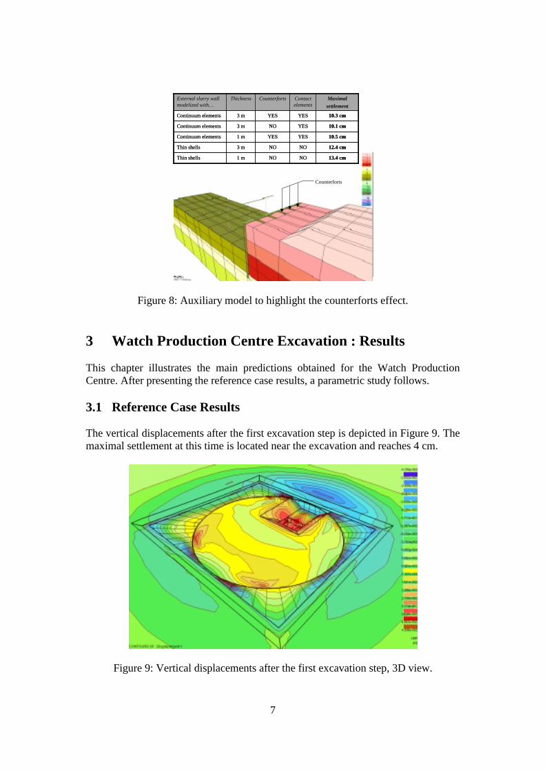
The external slurry wall is reinforced by counterforts in the execution project. Introducing each counterfort into the global 3D mesh would have been too tedious. An auxiliary analysis has therefore been conducted on a smaller part of the wall in order to estimate the influence of the absence of the counterforts (see Figure 8). Results show that settlements are overestimated by 20 to 30 % when modelling the wall with thin shells; the general behaviour of the retaining system is however correctly reproduced.

In the global analysis (§ 3), the thickness of the shells modelling the external

slurry wall varies between 1 meter (no counterfort) and 3 meters (continuous counterfort all around the excavation). The real wall’s behaviour will lie in between these two limit cases (variation : about 15 %).

7

Counterforts

1 m

3 m

1 m

3 m

3 m

Thickness

NO

NO

YES

NO

YES

Counterforts

Thin shells

Thin shells

Continuum elements

Continuum elements

Continuum elements

External slurry wall modelized with…

NO

NO

YES

YES

YES

Contact elements

13.4 cm

12.4 cm

10.5 cm

10.1 cm

10.3 cm

Maximalsettlement

1 m

3 m

1 m

3 m

3 m

Thickness

NO

NO

YES

NO

YES

Counterforts

Thin shells

Thin shells

Continuum elements

Continuum elements

Continuum elements

External slurry wall modelized with…

NO

NO

YES

YES

YES

Contact elements

13.4 cm

12.4 cm

10.5 cm

10.1 cm

10.3 cm

Maximalsettlement

Figure 8: Auxiliary model to highlight the counterforts effect.

3 Watch Production Centre Excavation : Results This chapter illustrates the main predictions obtained for the Watch Production Centre. After presenting the reference case results, a parametric study follows. 3.1 Reference Case Results The vertical displacements after the first excavation step is depicted in Figure 9. The maximal settlement at this time is located near the excavation and reaches 4 cm.

Figure 9: Vertical displacements after the first excavation step, 3D view.

8

Figure 10 illustrates the settlements around the excavation (and also the swelling of the subgrade) at the end of the earthworks. A maximal settlement of about 7 cm is predicted 30 m behind the external slurry wall.

Figure 10: Settlements at the end of the earthworks, top view.

Two cuts displaying the vertical displacement are given in Figure 11. The first cut is made just behind the northern slurry wall and the second cut crosses the excavation through the main technical gallery.

Figure 11: Settlements at the end of the earthworks, vertical cuts.

9

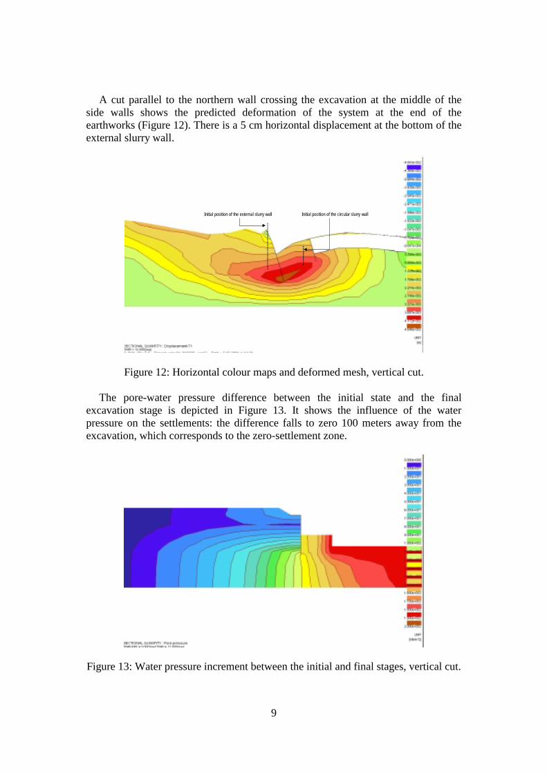
A cut parallel to the northern wall crossing the excavation at the middle of the side walls shows the predicted deformation of the system at the end of the earthworks (Figure 12). There is a 5 cm horizontal displacement at the bottom of the external slurry wall.

Initial position of the external slurry wall Initial position of the circular slurry wallInitial position of the external slurry wall Initial position of the circular slurry wall

Figure 12: Horizontal colour maps and deformed mesh, vertical cut.

The pore-water pressure difference between the initial state and the final excavation stage is depicted in Figure 13. It shows the influence of the water pressure on the settlements: the difference falls to zero 100 meters away from the excavation, which corresponds to the zero-settlement zone.

Figure 13: Water pressure increment between the initial and final stages, vertical cut.

10

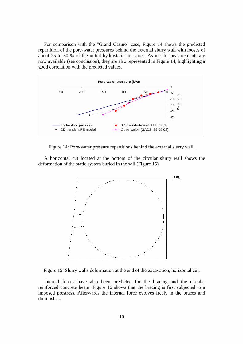
For comparison with the "Grand Casino" case, Figure 14 shows the predicted repartition of the pore-water pressures behind the external slurry wall with looses of about 25 to 30 % of the initial hydrostatic pressures. As in situ measurements are now available (see conclusion), they are also represented in Figure 14, highlighting a good correlation with the predicted values.

-25

-20

-15

-10

-5

0050100150200250

Pore-water pressure (kPa)

Dept

h (m

)

Hydrostatic pressure 3D pseudo-transient FE model 2D transient FE model Observation (GADZ, 29.05.02)

Figure 14: Pore-water pressure repartitions behind the external slurry wall.

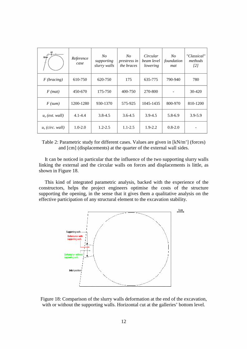
A horizontal cut located at the bottom of the circular slurry wall shows the deformation of the static system buried in the soil (Figure 15).

5 cm5 cm5 cm5 cm

Figure 15: Slurry walls deformation at the end of the excavation, horizontal cut. Internal forces have also been predicted for the bracing and the circular

reinforced concrete beam. Figure 16 shows that the bracing is first subjected to a imposed prestress. Afterwards the internal force evolves freely in the braces and diminishes.

11

Figure 16: Evolution of the compression inside the braces during the excavation.

3.2.2 Parametrical Study Modifications on the reference case are discussed next. The following changes are scrutinized:

• no auxiliary supporting slurry walls (see Figure 6) • no prestress in the braces • circular beam level lowering (- 2 meters) • no "instantaneous" foundation mat

Forces acting in the static system (Figure 17) and corresponding predicted

displacements are summarized in Table 2 for the afore-mentioned cases and compared to classical calculation methods involving simplifications.

F (bracing)

F (mat)

F (circular wall)

F (angle br.)

F (gallery mat)

ux (external wall)

ux (circular wall)

F (sum)

F (bracing)

F (mat)

F (circular wall)

F (angle br.)

F (gallery mat)

ux (external wall)

ux (circular wall)

F (sum)

Figure 17: Forces acting in the static system.

12

A2

B2

A2

B2

Reference case

No supporting slurry walls

No prestress in the braces

Circular beam level lowering

No foundation

mat

"Classical" methods

[2]

F (bracing) 610-750 620-750 175 635-775 790-940 780

F (mat) 450-670 175-750 400-750 270-800 - 30-420

F (sum) 1200-1280 930-1370 575-925 1045-1435 800-970 810-1200

ux (ext. wall) 4.1-4.4 3.8-4.5 3.6-4.5 3.9-4.5 5.8-6.9 3.9-5.9

ux (circ. wall) 1.0-2.0 1.2-2.5 1.1-2.5 1.9-2.2 0.8-2.0 -

Table 2: Parametric study for different cases. Values are given in [kN/m’] (forces)

and [cm] (displacements) at the quarter of the external wall sides.

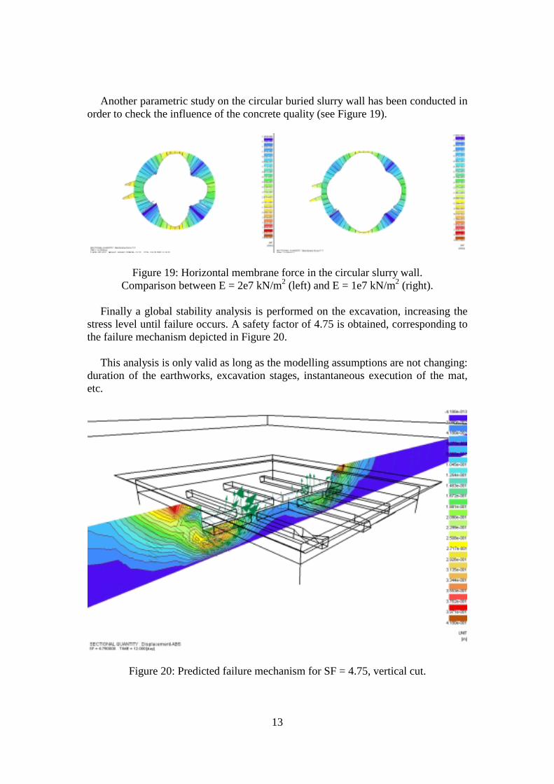
It can be noticed in particular that the influence of the two supporting slurry walls linking the external and the circular walls on forces and displacements is little, as shown in Figure 18.

This kind of integrated parametric analysis, backed with the experience of the

constructors, helps the project engineers optimise the costs of the structure supporting the opening, in the sense that it gives them a qualitative analysis on the effective participation of any structural element to the excavation stability.

5 cm

Initial position

Deformation withsupporting walls

Deformation withoutsupporting walls

Supporting walls

5 cm5 cm

Initial position

Deformation withsupporting walls

Deformation withoutsupporting walls

Supporting walls

Figure 18: Comparison of the slurry walls deformation at the end of the excavation, with or without the supporting walls. Horizontal cut at the galleries’ bottom level.

13

Another parametric study on the circular buried slurry wall has been conducted in order to check the influence of the concrete quality (see Figure 19).

Figure 19: Horizontal membrane force in the circular slurry wall. Comparison between E = 2e7 kN/m2 (left) and E = 1e7 kN/m2 (right).

Finally a global stability analysis is performed on the excavation, increasing the

stress level until failure occurs. A safety factor of 4.75 is obtained, corresponding to the failure mechanism depicted in Figure 20.

This analysis is only valid as long as the modelling assumptions are not changing:

duration of the earthworks, excavation stages, instantaneous execution of the mat, etc.

Figure 20: Predicted failure mechanism for SF = 4.75, vertical cut.

14

Conclusion In this paper we describe a 3D numerical simulation of a large excavation, including all the components of the project (hydro-geotechnical conditions, soil-structure interaction, excavation phases). This excavation is currently under construction, and the first set of in situ measures (inclinometers, pore-pressure cells, optical fibers) have just been analysed.

Of course, modifications have occurred, in particular the excavation steps have been changed. A new calculation incorporating better the reality would be necessary, to allow a rigorous comparison.

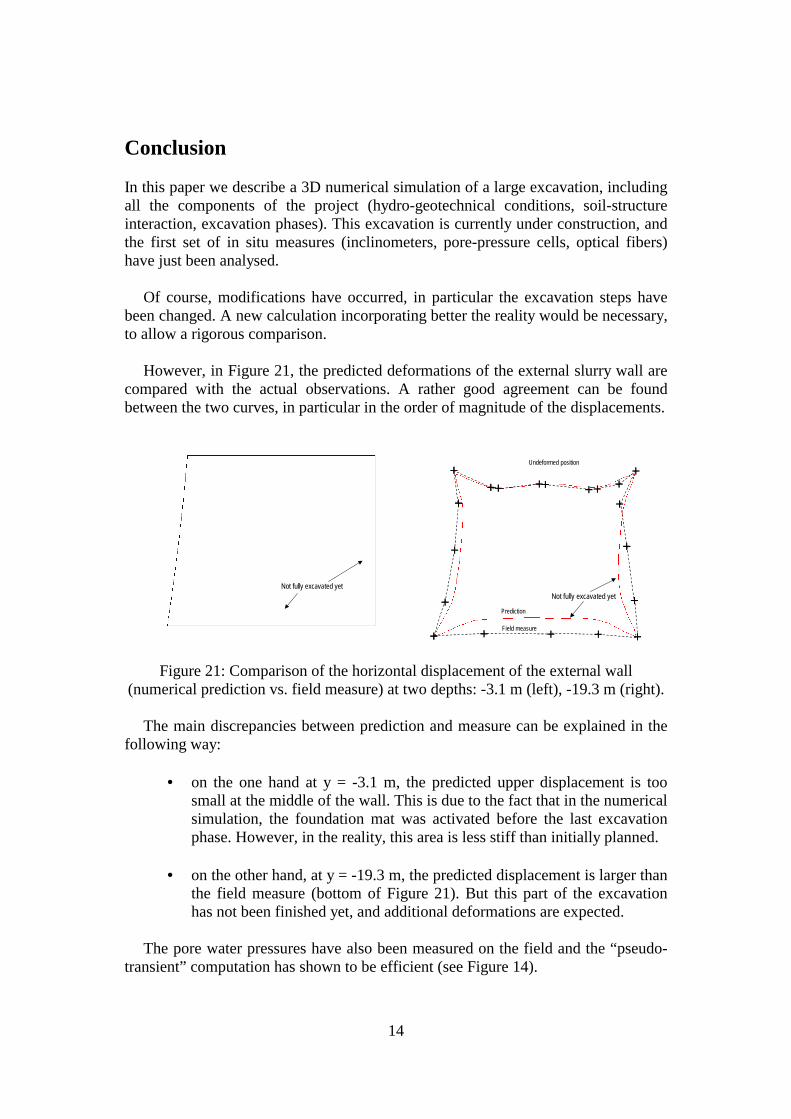
However, in Figure 21, the predicted deformations of the external slurry wall are

compared with the actual observations. A rather good agreement can be found between the two curves, in particular in the order of magnitude of the displacements.

2 cm

Undeformed position

Field measure

Prediction

Not fully excavated yet

4 cm

Undeformed position

Field measure

Prediction

Not fully excavated yet

Figure 21: Comparison of the horizontal displacement of the external wall (numerical prediction vs. field measure) at two depths: -3.1 m (left), -19.3 m (right).

The main discrepancies between prediction and measure can be explained in the following way:

• on the one hand at y = -3.1 m, the predicted upper displacement is too

small at the middle of the wall. This is due to the fact that in the numerical simulation, the foundation mat was activated before the last excavation phase. However, in the reality, this area is less stiff than initially planned.

• on the other hand, at y = -19.3 m, the predicted displacement is larger than

the field measure (bottom of Figure 21). But this part of the excavation has not been finished yet, and additional deformations are expected.

The pore water pressures have also been measured on the field and the “pseudo-

transient” computation has shown to be efficient (see Figure 14).

15

To conclude, this paper shows the importance of having complete initial data at hand for a 3D numerical simulation. The use of a real-scale test is also shown to be very useful in order to calibrate the parameters influencing most of the simulations, in particular the pore-water pressure decrease and the soil compressibilities leading to the necessity to choose an adapted constitutive law (Cap model). The time-consuming aspect of 3D numerical simulations can be reduced in conducting different parallel studies (influence of the counterforts, pseudo-transient calculation, no interface elements).

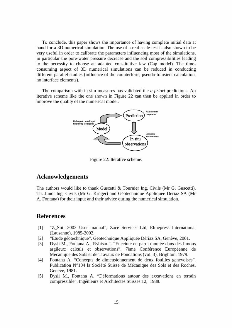
The comparison with in situ measures has validated the a priori predictions. An

iterative scheme like the one shown in Figure 22 can then be applied in order to improve the quality of the numerical model.

Model

Prediction

In situobservations

Hydro-geotechnical inputSimplifying assumptions

Finite elementcomputation

Excavationinstrumentation

Model

Prediction

In situobservations

Hydro-geotechnical inputSimplifying assumptions

Finite elementcomputation

Excavationinstrumentation

Figure 22: Iterative scheme. Acknowledgements The authors would like to thank Guscetti & Tournier Ing. Civils (Mr G. Guscetti), Th. Jundt Ing. Civils (Mr G. Krüger) and Géotechnique Appliquée Dériaz SA (Mr A. Fontana) for their input and their advice during the numerical simulation. References [1] “Z_Soil 2002 User manual”, Zace Services Ltd, Elmepress International

(Lausanne), 1985-2002. [2] “Etude géotechnique”, Géotechnique Appliquée Dériaz SA, Genève, 2001. [3] Dysli M., Fontana A., Rybisar J. “Enceinte en paroi moulée dans des limons

argileux: calculs et observations”. 7ème Conférence Européenne de Mécanique des Sols et de Travaux de Fondations (vol. 3), Brighton, 1979.

[4] Fontana A. “Concepts de dimensionnement de deux fouilles genevoises”. Publication N°104 la Société Suisse de Mécanique des Sols et des Roches, Genève, 1981.

[5] Dysli M., Fontana A. “Déformations autour des excavations en terrain compressible”. Ingénieurs et Architectes Suisses 12, 1988.