Numerical Simulation of Fractional Order Dengue … · Numerical Simulation of Fractional Order Dengue Disease with Incubation Period of Virus Zain Ul Abadin Zafar*1, 3, M. Mushtaq1,

Numerical Simulation of Fractional Order Dengue Disease with Incubation Period of Virus

Zain Ul Abadin Zafar*1, 3, M. Mushtaq1, Kashif Rehan2, and M. Rafiq4

1Department of Mathematics, University of Engineering and Technology, Lahore, Pakistan

2Department of Mathematics, University of Engineering and Technology, KSK Campus, Lahore, Pakistan 3Faculty of Information Technology, University of Central Punjab, Lahore, Pakistan

4Faculty of Engineering, University of Central Punjab, Lahore, Pakistan

Abstract: Nowadays, numerical models have great importance in epidemiology. These helps us to understand the transmission dynamics of infectious diseases in a very comprehensive manner. In disease epidemiology, vector-host models are important because many diseases are spreading through vectors. Mosquitoes are vectors of dengue disease as these spread the disease in a population. The infectious vectors infect the hosts while infectious hosts infect to vectors .Two main groups of dengue patients are septic and contagious. The susceptible mosquitoes can get dengue infection from infectious humans but not from infected ones. Humans can be categorized into Susceptible, infected, infectious and recovered ones while mosquitoes are susceptible, infected and infectious. Susceptible individual can transfer dengue infection from diseased mosquitoes only. The transmission dynamics of “Fractional order dengue fever” with incubation period of virus has been analyzed in this paper. Using standard methods for analyzing a system, the stability of equilibrium points of the model has been determined. Finally, numerical simulation has been performed for the same problem for different values of discretization parameter ‘h’.

Keywords: Dengue virus, incubation period, stability, fraction order numerical modeling

1. INTRODUCTION Recently, diseases caused by dengue virus have become a major health problem in the world [1]. Most probably these diseases are found in tropical areas and also found in some sub-tropical areas [2]. These diseases are found in the following countries America, Africa, Western Pacific, South Asia and Eastern Mediterranean. Before 1970 there were only nine countries which were affected by the dengue disease but after 1995 it increased four times. Until 2001 there were 609,000 patients affected by this disease. This number of patients is double to the figure as in 1995. Now major population of the world is at risk due to this disease. World Health Organization estimated that 49 M (Million) patients can be affected each year by this disease. The attack rate of this disease is 40-50% that can reach up to 80%-90% very soon. The dengue disease can be classified into three different types which are dengue hemorrhagic fever, dengue shock syndrome and dengue fever. These types have different symptoms. Dengue Fever symptoms are less in appearance in case of children’s while these appear in case of young and grown up children. Dengue hemorrhagic fever is one of the complex diseases which can turn into fatal condition. This type of disease occurs to the patient when a patient is prone to the dengue virus more than once. Dengue shock syndrome (DSS) is a severe type of which can lead the patient to the hospitalization. 1.1 Causes It can be caused by DEN1 – 4 virus.

Research Article

Proceedings of the Pakistan Academy of Sciences: Pakistan Academy of SciencesA. Physical and Computational Sciences 54 (3): 277–296 (2017)Copyright © Pakistan Academy of SciencesISSN: 2518-4245 (print), 2518-4253 (online)

————————————————Received, August 2016; Accepted, September 2017*Corresponding author: Zain Ul Abadin Zafar; Email: [email protected]

1.2 Transmission

The main cause of dengue disease is Aedes mosquito. After biting the infected human, it becomes infected with this disease and then that disease will be transmitted to other human beings. There are two types of Aedes mosquitoes which cause this disease. These types are: Aedes aegypti and Aedes albopictus. When the mosquito Aedes aegypti recruits with a dengue infectious person, the dengue virus enters the blood and circulate in the blood (viremia) that carry on for roughly four to seven days [3, 4]. Dengue cannot be transmitted directly from one person to another person. It needs a mosquito as transmitter from one person to another. Mosquitoes are only infected by this disease by biting an infected person. Virus replicates within the mosquito during the incubation period of 8-12 days. After this, glands of mosquito become infected and then virus of this disease will be transmitted to other person after biting that person. Then virus replicates in this newly infected person during the incubation period [5].

1.3 Symptoms

Its symptoms are 4 to 7 days fever after a person has been attacked by mosquito infected with virus. Symptoms are retro-orbital pain nausea, severe headache, joint and muscle pain, rashes, vomiting & high fever. DHF includes all symptoms of dengue fever with some additional symptoms which are bleeding from the nose, gums, or under the skin. It is severe form of dengue which can lead to death.

2. MODEL FORMATION

2.1 Assumptions

• The number of human and mosquito remains same. • DEN virus effete gets permanent protection from the particular virus but becomes sensitive for

others. • Death and birth rate of human and mosquito goes on side by side.

Variables for model are that represents some special notions are as follow:

𝑆𝑆ℎ̅(𝑡𝑡) represents the susceptible individuals with in time 𝑡𝑡, 𝑋𝑋�ℎ(𝑡𝑡) denotes the Infected individuals with in time 𝑡𝑡, 𝐼𝐼ℎ̅(𝑡𝑡) gives the number of Infectious individuals with in time 𝑡𝑡 and 𝑅𝑅�ℎ(𝑡𝑡) are Recovered individuals with in time 𝑡𝑡. Beside these 𝑆𝑆�̅�𝑣(𝑡𝑡) are the Susceptible mosquitoes (vectors) with in time 𝑡𝑡, 𝑋𝑋�𝑣𝑣(𝑡𝑡) tells the Infected mosquitoes (vectors) with in time 𝑡𝑡, and 𝐼𝐼�̅�𝑣(𝑡𝑡) gives the number of Infectious mosquitoes with in time 𝑡𝑡.

2.2 Mathematical Model

The transmission of dengue virus is shown by following flow chart [6].

The following equations describe transmission dynamics of Dengue infection in human and vector populations:

278 Zain Ul Abadin Zafar et al

𝑑𝑑�̅�𝑆ℎ𝑑𝑑𝑑𝑑

= 𝜆𝜆𝑁𝑁𝑇𝑇 − 𝛽𝛽ℎ𝑆𝑆ℎ̅𝐼𝐼�̅�𝑣 − µℎ𝑆𝑆ℎ̅𝑑𝑑𝑋𝑋�ℎ𝑑𝑑𝑑𝑑

= 𝛽𝛽ℎ𝑆𝑆ℎ̅𝐼𝐼�̅�𝑣 − 𝛼𝛼ℎ𝑋𝑋�ℎ − µℎ𝑋𝑋�ℎ𝑑𝑑𝐼𝐼ℎ̅𝑑𝑑𝑑𝑑

= 𝛼𝛼ℎ𝑋𝑋�ℎ − 𝑟𝑟𝐼𝐼ℎ̅ − µℎ𝐼𝐼ℎ̅𝑑𝑑𝑅𝑅�ℎ𝑑𝑑𝑑𝑑

= 𝑟𝑟𝐼𝐼ℎ̅ − µℎ𝑅𝑅�ℎ

𝑑𝑑�̅�𝑆𝑣𝑣𝑑𝑑𝑑𝑑

= 𝐶𝐶 − 𝛽𝛽𝑣𝑣𝐼𝐼ℎ̅𝑆𝑆�̅�𝑣 − µ𝑣𝑣𝑆𝑆�̅�𝑣𝑑𝑑𝑋𝑋�𝑣𝑣𝑑𝑑𝑑𝑑

= 𝛽𝛽𝑣𝑣𝐼𝐼ℎ̅𝑆𝑆�̅�𝑣–𝛼𝛼𝑣𝑣𝑋𝑋�𝑣𝑣 − µ𝑣𝑣𝑋𝑋�𝑣𝑣𝑑𝑑𝐼𝐼�̅�𝑣𝑑𝑑𝑑𝑑

= 𝛼𝛼𝑣𝑣𝑋𝑋�𝑣𝑣 − µ𝑣𝑣𝐼𝐼�̅�𝑣 ⎭⎪⎪⎪⎪⎬

⎪⎪⎪⎪⎫

(1)

with 𝑁𝑁𝑇𝑇 = 𝑆𝑆ℎ̅ + 𝑋𝑋�ℎ + 𝐼𝐼ℎ̅ + 𝑅𝑅�ℎ

and 𝑁𝑁𝑣𝑣 = 𝑆𝑆�̅�𝑣 + 𝑋𝑋�𝑣𝑣 + 𝐼𝐼�̅�𝑣

where 𝑁𝑁𝑇𝑇 and 𝑁𝑁𝑣𝑣 are constant. So,

𝑑𝑑𝑁𝑁𝑇𝑇𝑑𝑑𝑑𝑑

= 0 and 𝑑𝑑𝑁𝑁𝑣𝑣𝑑𝑑𝑑𝑑

= 0

which implies that 𝜆𝜆 = µℎ

Now for vector population 𝑑𝑑𝑁𝑁𝑣𝑣𝑑𝑑𝑑𝑑

=𝑑𝑑𝑑𝑑𝑑𝑑

(𝑆𝑆�̅�𝑣 + 𝑋𝑋�𝑣𝑣 + 𝐼𝐼�̅�𝑣)

0 =𝑑𝑑𝑑𝑑𝑑𝑑𝑆𝑆�̅�𝑣 +

𝑑𝑑𝑑𝑑𝑑𝑑𝑋𝑋�𝑣𝑣 +

𝑑𝑑𝑑𝑑𝑑𝑑𝐼𝐼�̅�𝑣

0 = 𝐶𝐶 − µ𝑣𝑣𝑆𝑆�̅�𝑣 − µ𝑣𝑣𝑋𝑋�𝑣𝑣 − µ𝑣𝑣𝐼𝐼�̅�𝑣

0 = 𝐶𝐶 − µ𝑣𝑣(𝑆𝑆�̅�𝑣 − 𝑋𝑋�𝑣𝑣 − 𝐼𝐼�̅�𝑣)

0 = 𝐶𝐶 − µ𝑣𝑣𝑁𝑁𝑣𝑣 ⇒ 𝑁𝑁𝑣𝑣 = 𝐶𝐶µ𝑣𝑣

For normalization of system (1), we let

𝑆𝑆 = �̅�𝑆ℎNT

, 𝑋𝑋 = 𝑋𝑋�ℎNT

, 𝐼𝐼 = 𝐼𝐼ℎ̅NT

, 𝑅𝑅 = 𝑅𝑅�ℎNT

𝑆𝑆𝑣𝑣 = �̅�𝑆𝑣𝑣NT

, 𝑋𝑋𝑣𝑣 = 𝑋𝑋�𝑣𝑣NT

, 𝐼𝐼𝑣𝑣 = 𝐼𝐼�̅�𝑣NT

The system of differential equation for transmission dynamics of dengue fever in normalized form is

𝑑𝑑𝑑𝑑𝑑𝑑𝑑𝑑

= µℎ − 𝛽𝛽ℎS𝐼𝐼𝑣𝑣 (C/µ𝑣𝑣)− µℎ𝑆𝑆

𝑑𝑑𝑋𝑋𝑑𝑑𝑑𝑑

= βℎS𝐼𝐼𝑣𝑣 (C/µ𝑣𝑣) − 𝛼𝛼ℎ𝑋𝑋 − µℎ𝑋𝑋𝑑𝑑𝐼𝐼𝑑𝑑𝑑𝑑

= 𝛼𝛼ℎ𝑋𝑋 − 𝑟𝑟𝐼𝐼 − µℎ𝐼𝐼 𝑑𝑑𝑋𝑋𝑣𝑣𝑑𝑑𝑑𝑑

= 𝛽𝛽𝑣𝑣𝐼𝐼𝑁𝑁𝑇𝑇(1 − 𝑋𝑋𝑣𝑣 − 𝐼𝐼𝑣𝑣) − 𝛼𝛼𝑣𝑣𝑋𝑋𝑣𝑣 − µ𝑣𝑣𝑋𝑋𝑣𝑣𝑑𝑑𝐼𝐼𝑣𝑣𝑑𝑑𝑑𝑑

= 𝛼𝛼𝑣𝑣𝑋𝑋𝑣𝑣 − µ𝑣𝑣𝐼𝐼𝑣𝑣 ⎭⎪⎪⎬

⎪⎪⎫

(2)

Fractional Order Dengue Disease 279

subject to the conditions: 𝑆𝑆 + 𝑋𝑋 + 𝐼𝐼 + 𝑅𝑅 = 1 and 𝑆𝑆𝑣𝑣 + 𝑋𝑋𝑣𝑣 + 𝐼𝐼𝑣𝑣 = 1

The terminology used for the different parameters are given Table 1. Table 1. Different symbols and terminology. Symbol Terminology

𝑁𝑁𝑇𝑇 Total population of human 𝛽𝛽ℎ Infectious rate of dengue virus from mosquitoes (vector) to human population 𝜆𝜆 Human population’s birth rate 𝛽𝛽𝑣𝑣 Infectious rate of dengue virus from human to mosquito (vector) population 𝛼𝛼ℎ Rate of changing the infected human population to infectious human population 𝑅𝑅 Human population’s recovery rate µℎ Human population death rate 𝛼𝛼𝑣𝑣 Vector (mosquito) population death rate 𝐶𝐶 Vector (mosquito) population constant recruitment rate

3. BEGINNINGS AND CYPHERS

In this segment, some simple explanations and chattels of the fractional calculus theory and Non-standard discretization are discussed.

3.1. Fundamentals of Fractional-order Fractional calculus represents a generalization of the ordinary differentiation and integration to non-integer and complex order [22]. The generalization of differential calculus to non-integer orders of derivatives can be traced back to Leibnitz [24]. The main reason for using integer order models was the absence of solution methods for fractional differential equations. It is an emerging field in the area of applied mathematics and mathematical physics such as chemistry, biology, economics, image and signal processing and it has many applications in many areas of science and engineering [23] for example, viscoelasticity, control theory, heat conduction, electricity, chaos and fractals etc. [22]. Various applications, like in the reaction kinetics of proteins, the anomalous electron transport in amorphous materials, the dielectrical or mechanical relation of polymers, the modeling of glass forming liquids and others are successfully performed in numerous papers [24]. The physical and geometrical meaning of the non-integer integral containing the real and complex conjugate power-law exponent has been proposed. Finding examples of real systems describes by the fractional derivative is an open issue in the area of fractional calculus [22]. Since integer order differential equations cannot precisely describe the experimental and field measurement data, as an alternative approach non-integer order differential equation models are now being widely applied [ 19, 20].The advantage of fractional-order differential equation systems over ordinary differential equation systems is that they allow greater degrees of freedom and incorporate memory effect in the model. In other words, it provides an excellent tool for the description of memory and hereditary properties which were not taken into account in the classical integer order model [21]. The calculus of variations is widely applied for some disciplines like engineering, pure and applied mathematics. Moreover, the researchers have recently proved that the physical systems with dissipation can be clearly modeled more accurately by using fractional representations [23]. Recently, most of the dynamical systems based on the integer-order calculus have been modified into the fractional order domain due to the extra degrees of freedom and the flexibility which can be used to precisely fit the experimental data much better than the integer order modeling. Few of the nonlinear models are given in [28-30].


There are many definitions of fractional derivatives. Few of them are:

(1) Caputo’s definition [25]

𝔇𝔇𝑢𝑢𝜙𝜙�𝑔𝑔(𝑢𝑢)� = 1

Γ(𝑛𝑛−𝜙𝜙)∫ (𝑢𝑢 − 𝑠𝑠)𝑛𝑛−𝜙𝜙−1𝑢𝑢0

𝑑𝑑𝑛𝑛𝑔𝑔(𝑠𝑠)𝑑𝑑𝑠𝑠𝑛𝑛

𝑑𝑑𝑠𝑠

(2) Riemann-Liouville definition [25]


Γ(𝑛𝑛−𝜙𝜙)𝑑𝑑𝑛𝑛

𝑑𝑑𝑢𝑢𝑛𝑛 ∫ (𝑢𝑢 − 𝑠𝑠)𝑛𝑛−𝜙𝜙−1𝑢𝑢0 𝑔𝑔(𝑠𝑠) 𝑑𝑑𝑠𝑠

(3) Jumarie’s definition [25]


Γ(𝑛𝑛−𝜙𝜙)𝑑𝑑𝑛𝑛

𝑑𝑑𝑢𝑢𝑛𝑛 ∫ (𝑢𝑢 − 𝑠𝑠)𝑛𝑛−𝜙𝜙−1𝑢𝑢0 [𝑔𝑔(𝑠𝑠) − 𝑔𝑔(0)] 𝑑𝑑𝑠𝑠

(4) Xiao-Jun Yang’s definition [25]

𝔇𝔇𝑢𝑢𝜙𝜙�𝑔𝑔(𝑢𝑢0)� = 𝑔𝑔𝜙𝜙(𝑢𝑢0) = 𝑑𝑑𝜙𝜙

𝑑𝑑𝑢𝑢𝜙𝜙𝑔𝑔(𝑢𝑢)�

𝑢𝑢=𝑢𝑢0= lim𝑢𝑢→𝑢𝑢0

∆𝜙𝜙(𝑔𝑔(𝑢𝑢)−𝑔𝑔(𝑢𝑢0))(𝑢𝑢−𝑢𝑢0)𝜙𝜙

where ∆𝜙𝜙�𝑔𝑔(𝑢𝑢) − 𝑔𝑔(𝑢𝑢0)� ≅ Γ (1 + 𝜙𝜙)Δ(𝑔𝑔(𝑢𝑢) − 𝑔𝑔(𝑢𝑢0)).

(5) Chen’s fractal derivative [25]

𝑑𝑑𝑔𝑔𝑑𝑑𝑢𝑢𝜙𝜙

= lim𝑠𝑠→𝑢𝑢𝑔𝑔(𝑢𝑢)−𝑔𝑔(𝑠𝑠)𝑢𝑢𝜙𝜙−𝑠𝑠𝜙𝜙

(6) Ji-Huan He’s fractal derivative [25]

𝔇𝔇𝑔𝑔𝔇𝔇𝑢𝑢𝜙𝜙

= Γ (1 + 𝜙𝜙) limΔ𝑢𝑢=𝑢𝑢1−𝑢𝑢2→𝐿𝐿𝑔𝑔(𝑢𝑢1)−𝑔𝑔(𝑢𝑢2)

(𝑢𝑢1−𝑢𝑢2)𝜙𝜙

where Δ𝑢𝑢 does not tend to zero, it can be the thickness (𝐿𝐿) of a porous medium. Applications of the fractal derivative to fractal media have attracted much attention, for example it can model heat transfer and water permeation in multi-scale of fabrics and wool fibers.

(7) Davidson-Essex derivative [26]

𝔇𝔇0𝜙𝜙�𝑔𝑔(𝑢𝑢)� = 1

Γ(1−𝜙𝜙)𝑑𝑑𝑛𝑛+1−𝑘𝑘

𝑑𝑑𝑢𝑢𝑛𝑛+1−𝑘𝑘 ∫ (𝑢𝑢 − 𝑠𝑠)−𝜙𝜙𝑢𝑢0 𝑑𝑑

𝑘𝑘𝑔𝑔(𝑠𝑠)𝑑𝑑𝑠𝑠𝑘𝑘

𝑑𝑑𝑠𝑠

(8) Coimbra derivative [26]

𝔇𝔇0𝜙𝜙(𝑢𝑢)�𝑔𝑔(𝑢𝑢)� = 1

Γ(1−𝜙𝜙(𝑢𝑢))�∫ (𝑢𝑢 − 𝑠𝑠)−𝜙𝜙(𝑥𝑥)𝑢𝑢0 𝑑𝑑𝑔𝑔(𝑠𝑠)

𝑑𝑑𝑠𝑠 𝑑𝑑𝑠𝑠 + 𝑔𝑔(0)𝑢𝑢−𝜙𝜙(𝑢𝑢)�

(9) Canavati derivative [26]

𝔇𝔇𝑎𝑎 𝑢𝑢𝜉𝜉�𝑔𝑔(𝑢𝑢)� = 1

Γ(1−𝜙𝜙)𝑑𝑑𝑑𝑑𝑢𝑢 ∫ (𝑢𝑢 − 𝑠𝑠)𝜙𝜙𝑢𝑢

0 𝑑𝑑𝑛𝑛𝑔𝑔(𝑠𝑠)𝑑𝑑𝑠𝑠𝑛𝑛

𝑑𝑑𝑠𝑠

𝑛𝑛 = |𝜉𝜉|, 𝜙𝜙 = 𝑛𝑛 − 𝜉𝜉

(10) Osler fractional derivative [26]

𝔇𝔇𝑎𝑎 𝑢𝑢𝜉𝜉�𝑔𝑔(𝑢𝑢)� = Γ(1+𝜙𝜙)

2π i ∫ 𝑔𝑔(𝑠𝑠)(𝑠𝑠−𝑢𝑢)1+𝜙𝜙𝔖𝔖(𝑎𝑎,𝑢𝑢+) 𝑑𝑑𝑠𝑠

(11) k-fractional Hilfer derivative [26]

𝔇𝔇𝜙𝜙,𝜉𝜉𝑘𝑘 �𝑔𝑔(𝑢𝑢)� = 𝐼𝐼𝑘𝑘𝜉𝜉(1−𝜙𝜙) 𝑑𝑑

𝑑𝑑𝑢𝑢𝐼𝐼𝑘𝑘

(1−𝜉𝜉)(1−𝜙𝜙) 𝑔𝑔(𝑢𝑢)

where 𝐼𝐼𝑘𝑘𝜙𝜙𝑔𝑔(𝑢𝑢) is the k-fractional Hilfer integral

𝐼𝐼𝑘𝑘𝜙𝜙𝑔𝑔(𝑢𝑢) = 1

𝑘𝑘 Γ𝑘𝑘(𝜙𝜙)∫ (𝑢𝑢 − 𝑠𝑠)𝜙𝜙𝑘𝑘−1𝑔𝑔(𝑢𝑢)𝑑𝑑𝑢𝑢𝑢𝑢

0

(12) Caputo Fabrizio derivative [27]


Let 𝑔𝑔 ∈ 𝐻𝐻1(𝑎𝑎, 𝑏𝑏), 𝑎𝑎 < 𝑏𝑏, 𝜙𝜙 ∈ [0,1] then, the new Caputo fractional derivative is

𝔇𝔇𝑢𝑢𝜙𝜙�𝑔𝑔(𝑢𝑢)� = 𝑀𝑀(𝜙𝜙)

1−𝜙𝜙 ∫ 𝑔𝑔′(𝑢𝑢)𝑢𝑢𝑎𝑎 exp �−𝜙𝜙 𝑢𝑢−𝑠𝑠

1−𝜙𝜙� 𝑑𝑑𝑑𝑑 (*)

where 𝑀𝑀(𝜙𝜙) enotes a normalization function obeying 𝑀𝑀(0) = 𝑀𝑀(1) = 1. However, if the function does not belong to 𝐻𝐻1(𝑎𝑎, 𝑏𝑏)then, the derivative has the form

𝔇𝔇𝑢𝑢𝜙𝜙�𝑔𝑔(𝑢𝑢)� = 𝜙𝜙𝑀𝑀(𝜙𝜙)

1−𝜙𝜙 ∫ [𝑔𝑔(𝑢𝑢) − 𝑔𝑔(𝑑𝑑)]𝑢𝑢𝑎𝑎 exp �−𝜙𝜙 𝑢𝑢−𝑠𝑠

1−𝜙𝜙� 𝑑𝑑𝑑𝑑 (**)

If 𝜎𝜎 = 1−𝜙𝜙𝜙𝜙

∈ [0,∞], 𝜙𝜙 = 11+𝜎𝜎

∈ [0,1], then eq. (**) assumes the form

𝔇𝔇𝑢𝑢𝜎𝜎�𝑔𝑔(𝑢𝑢)� = 𝑁𝑁(𝜎𝜎)

𝜎𝜎 ∫ 𝑔𝑔′(𝑢𝑢)𝑢𝑢𝑎𝑎 exp �− 𝑢𝑢−𝑠𝑠

𝜎𝜎� 𝑑𝑑𝑑𝑑 , 𝑁𝑁(0) = 𝑁𝑁(∞) = 1

(13) Atangana Baleanu Fractional Derivative in Riemann-Liouville sense[28]

Let 𝑔𝑔 ∈ 𝐻𝐻1(𝑎𝑎, 𝑏𝑏), 𝑎𝑎 < 𝑏𝑏, 𝜙𝜙 ∈ [0,1] and not necessary differentiable then, the definition of the new fractional derivative is given as

𝔇𝔇𝑎𝑎𝐴𝐴𝐴𝐴𝐴𝐴𝑢𝑢𝜙𝜙�𝑔𝑔(𝑢𝑢)� = 𝐴𝐴(𝜙𝜙)

1−𝜙𝜙𝑑𝑑𝑑𝑑𝑢𝑢 ∫ 𝑔𝑔(𝑑𝑑)𝑢𝑢

𝑎𝑎 E𝜙𝜙 �−𝜙𝜙(𝑢𝑢−𝑠𝑠)𝜙𝜙

1−𝜙𝜙� 𝑑𝑑𝑑𝑑

(14) Atangana Baleanu Fractional Derivative in Riemann-Caputo sense [28]

Let 𝑔𝑔 ∈ 𝐻𝐻1(𝑎𝑎, 𝑏𝑏), 𝑎𝑎 < 𝑏𝑏, 𝜙𝜙 ∈ [0,1] and not necessary differentiable then, the definition of the new fractional derivative is given as

𝔇𝔇𝑎𝑎𝐴𝐴𝐴𝐴𝐴𝐴𝑢𝑢𝜙𝜙�𝑔𝑔(𝑢𝑢)� = 𝐴𝐴(𝜙𝜙)

1−𝜙𝜙 ∫ 𝑔𝑔′(𝑑𝑑)𝑢𝑢𝑎𝑎 E𝜙𝜙 �−𝜙𝜙

(𝑢𝑢−𝑠𝑠)𝜙𝜙

1−𝜙𝜙� 𝑑𝑑𝑑𝑑

3.2. Grunwald-Letnikov (GL) Method

The GL method of approximation for the 1-D fractional derivative is as follows [11].

𝐷𝐷𝛽𝛽𝑥𝑥(𝜏𝜏) = 𝑔𝑔�𝜏𝜏, 𝑥𝑥(𝜏𝜏)�, 𝑥𝑥(0) = 𝑥𝑥0, 𝜏𝜏 ∈ [0, 𝜏𝜏𝑓𝑓], (3)

𝐷𝐷𝛽𝛽𝑥𝑥(𝜏𝜏) = limℎ→0 ℎ−𝛽𝛽 ∑ (−1)𝑖𝑖 �𝛽𝛽𝑖𝑖 ��𝜏𝜏𝑓𝑓𝒉𝒉 �𝒋𝒋=𝟎𝟎 𝑥𝑥(𝜏𝜏 − 𝑖𝑖ℎ),

where 0 < 𝛽𝛽 < 1, 𝐷𝐷𝛽𝛽 signifies the fractional derivative, ℎ is the step size and �𝜏𝜏𝑓𝑓ℎ� represents the integer

part of 𝜏𝜏𝑓𝑓𝒉𝒉

. Therefore, Eq. (3) is discretized in the next form,

∑ 𝐶𝐶𝑗𝑗𝛽𝛽𝑛𝑛

𝑖𝑖=0 𝑥𝑥𝑛𝑛−𝑗𝑗 = 𝑓𝑓(𝜏𝜏𝑛𝑛,𝑥𝑥𝑛𝑛), 𝑛𝑛 = 1,2,3, …

where 𝜏𝜏𝑛𝑛 = 𝑛𝑛ℎ and 𝐶𝐶𝑗𝑗𝛽𝛽 are the GL coefficients defined as

𝐶𝐶𝑖𝑖𝛽𝛽 = �1 − 1+𝛽𝛽

𝑖𝑖� 𝐶𝐶𝑖𝑖−1

𝛽𝛽 , 𝐶𝐶0𝛽𝛽 = ℎ−𝛽𝛽, 𝑖𝑖 = 1,2,3 …

The paper of Mickens [13] provides an all-purpose route for determining ∅(ℎ) for the ODEs. A specimen of the NSFD discretization procedure is its application to the decay equation

𝑥𝑥′ = −𝜆𝜆 𝑥𝑥

where 𝜆𝜆 is constant. The discretization scheme [13] is

𝑥𝑥𝑛𝑛+1−𝑥𝑥𝑛𝑛∅

= −𝜆𝜆 𝑥𝑥𝑛𝑛, ∅(ℎ, 𝜆𝜆 ) = 1−𝑒𝑒−𝜆𝜆 ℎ

𝜆𝜆

An alternate example is given by

𝑥𝑥′ = 𝜆𝜆1 𝑥𝑥 − 𝜆𝜆2 𝑥𝑥2


where the NSFD scheme is 𝑥𝑥𝑛𝑛+1 − 𝑥𝑥𝑛𝑛

∅= 𝜆𝜆1 𝑥𝑥𝑛𝑛 − 𝜆𝜆2𝑥𝑥𝑛𝑛𝑥𝑥𝑛𝑛+1

∅(ℎ, 𝜆𝜆1 ) =𝑒𝑒𝜆𝜆1 ℎ − 1

𝜆𝜆1

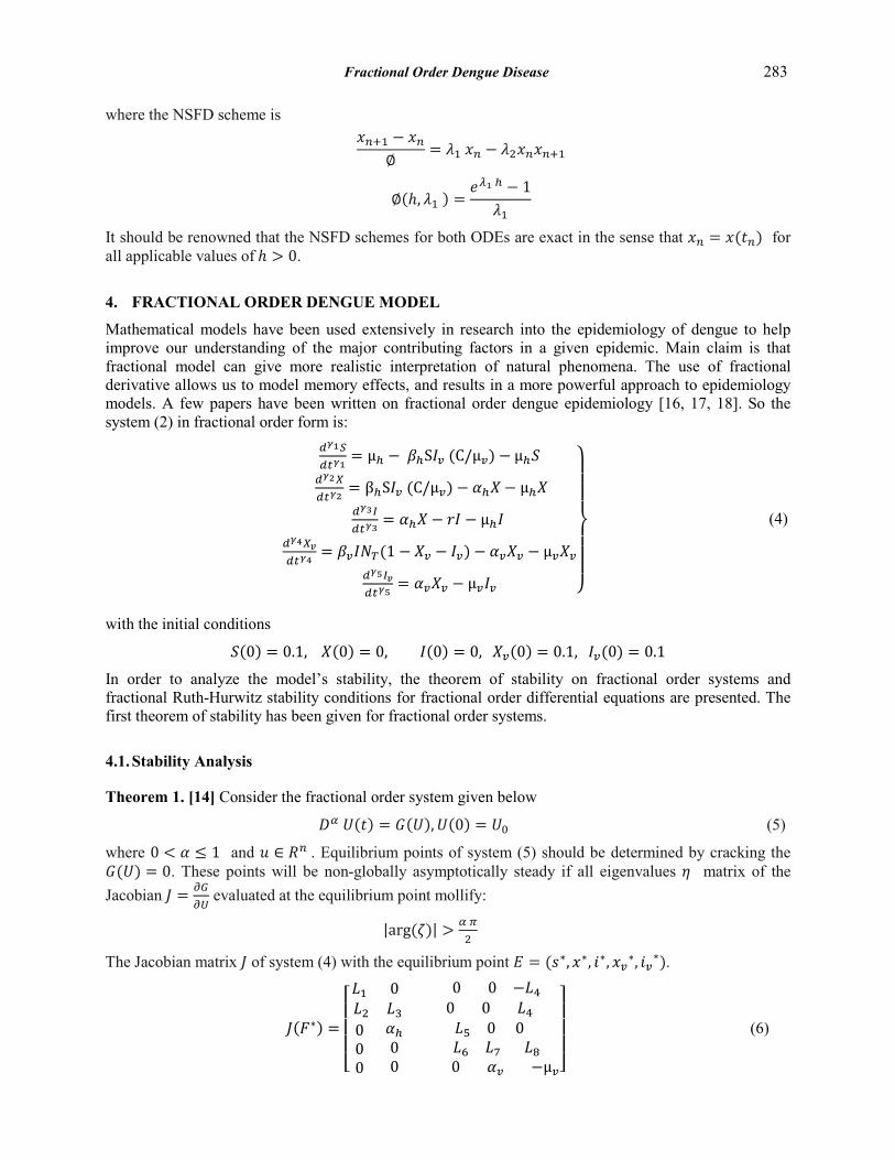
It should be renowned that the NSFD schemes for both ODEs are exact in the sense that 𝑥𝑥𝑛𝑛 = 𝑥𝑥(𝑡𝑡𝑛𝑛) for all applicable values of ℎ > 0.

4. FRACTIONAL ORDER DENGUE MODEL

Mathematical models have been used extensively in research into the epidemiology of dengue to help improve our understanding of the major contributing factors in a given epidemic. Main claim is that fractional model can give more realistic interpretation of natural phenomena. The use of fractional derivative allows us to model memory effects, and results in a more powerful approach to epidemiology models. A few papers have been written on fractional order dengue epidemiology [16, 17, 18]. So the system (2) in fractional order form is:

𝑑𝑑𝛾𝛾1𝑆𝑆𝑑𝑑𝑡𝑡𝛾𝛾1

= µℎ − 𝛽𝛽ℎS𝐼𝐼𝑣𝑣 (C/µ𝑣𝑣) − µℎ𝑆𝑆

𝑑𝑑𝛾𝛾2𝑋𝑋𝑑𝑑𝑡𝑡𝛾𝛾2

= βℎS𝐼𝐼𝑣𝑣 (C/µ𝑣𝑣) − 𝛼𝛼ℎ𝑋𝑋 − µℎ𝑋𝑋𝑑𝑑𝛾𝛾3𝐼𝐼𝑑𝑑𝑡𝑡𝛾𝛾3

= 𝛼𝛼ℎ𝑋𝑋 − 𝑟𝑟𝐼𝐼 − µℎ𝐼𝐼 𝑑𝑑𝛾𝛾4𝑋𝑋𝑣𝑣𝑑𝑑𝑡𝑡𝛾𝛾4

= 𝛽𝛽𝑣𝑣𝐼𝐼𝑁𝑁𝑇𝑇(1 − 𝑋𝑋𝑣𝑣 − 𝐼𝐼𝑣𝑣)− 𝛼𝛼𝑣𝑣𝑋𝑋𝑣𝑣 − µ𝑣𝑣𝑋𝑋𝑣𝑣𝑑𝑑𝛾𝛾5𝐼𝐼𝑣𝑣𝑑𝑑𝑡𝑡𝛾𝛾5

= 𝛼𝛼𝑣𝑣𝑋𝑋𝑣𝑣 − µ𝑣𝑣𝐼𝐼𝑣𝑣 ⎭⎪⎪⎪⎬

⎪⎪⎪⎫

(4)

with the initial conditions

𝑆𝑆(0) = 0.1, 𝑋𝑋(0) = 0, 𝐼𝐼(0) = 0, 𝑋𝑋𝑣𝑣(0) = 0.1, 𝐼𝐼𝑣𝑣(0) = 0.1

In order to analyze the model’s stability, the theorem of stability on fractional order systems and fractional Ruth-Hurwitz stability conditions for fractional order differential equations are presented. The first theorem of stability has been given for fractional order systems.

4.1. Stability Analysis

Theorem 1. [14] Consider the fractional order system given below

𝐷𝐷𝛼𝛼 𝑈𝑈(𝑡𝑡) = 𝐺𝐺(𝑈𝑈),𝑈𝑈(0) = 𝑈𝑈0 (5)

where 0 < 𝛼𝛼 ≤ 1 and 𝑢𝑢 ∈ 𝑅𝑅𝑛𝑛 . Equilibrium points of system (5) should be determined by cracking the 𝐺𝐺(𝑈𝑈) = 0. These points will be non-globally asymptotically steady if all eigenvalues 𝜂𝜂 matrix of the Jacobian 𝐽𝐽 = 𝜕𝜕𝜕𝜕

𝜕𝜕𝜕𝜕 evaluated at the equilibrium point mollify:

|arg (𝜁𝜁)| > 𝛼𝛼 𝜋𝜋2

The Jacobian matrix 𝐽𝐽 of system (4) with the equilibrium point 𝐸𝐸 = (𝑠𝑠∗,𝑥𝑥∗, 𝑖𝑖∗, 𝑥𝑥𝑣𝑣∗, 𝑖𝑖𝑣𝑣∗).

𝐽𝐽(𝐹𝐹∗) =

⎣⎢⎢⎢⎡𝐿𝐿1 0 0 0 −𝐿𝐿4 𝐿𝐿2 𝐿𝐿3 0 0 𝐿𝐿4000

𝛼𝛼ℎ00

𝐿𝐿5 0 0 𝐿𝐿6 𝐿𝐿7 𝐿𝐿8

0 𝛼𝛼𝑣𝑣 −µ𝑣𝑣⎦⎥⎥⎥⎤

(6)


𝐿𝐿1 = −βℎ𝑖𝑖𝑣𝑣∗𝐶𝐶µ𝑣𝑣

− µℎ , 𝐿𝐿2 =βℎ𝑖𝑖𝑣𝑣∗𝐶𝐶µ𝑣𝑣

, 𝐿𝐿3 = −µℎ − 𝛼𝛼ℎ ,𝐿𝐿4 =βℎ𝑠𝑠∗𝐶𝐶µ𝑣𝑣

, 𝐿𝐿5 = −µℎ − r,

𝐿𝐿6 = 𝛽𝛽𝑣𝑣𝑁𝑁𝑇𝑇(1 − 𝑥𝑥𝑣𝑣∗ − 𝑖𝑖𝑣𝑣∗), 𝐿𝐿7 = −𝛼𝛼𝑣𝑣 − µ𝑣𝑣 − 𝛽𝛽𝑣𝑣𝑖𝑖∗𝑁𝑁𝑇𝑇 , 𝐿𝐿8 = −𝛽𝛽𝑣𝑣𝑖𝑖∗𝑁𝑁𝑇𝑇

4.2. Equilibrium Points

To find the equilibrium state points we set the right hand side of all equations in system (4) equated to zero. We found that the system has two possible equilibrium points i.e. the disease free equilibrium (DFE) and endemic equilibrium (EE).

Disease free equilibrium (DFE):

𝑉𝑉0 = (1, 0, 0,0,0)

Endemic equilibrium (EE):

𝑉𝑉1 = (𝑆𝑆∗,𝑋𝑋∗, 𝐼𝐼∗,𝑋𝑋𝑣𝑣∗, 𝐼𝐼𝑣𝑣∗)

where

𝑆𝑆∗ =(𝛼𝛼𝑣𝑣 + µ𝑣𝑣)(𝑊𝑊𝑊𝑊µℎ2µ𝑣𝑣 + 𝛼𝛼ℎ 𝛾𝛾𝑣𝑣 µℎ)𝛼𝛼ℎ 𝛾𝛾𝑣𝑣 [µℎ(𝛼𝛼𝑣𝑣 + µ𝑣𝑣) + 𝛼𝛼𝑣𝑣𝛾𝛾ℎ ]

𝑋𝑋∗ =𝑊𝑊µℎ2µ𝑣𝑣(𝛼𝛼𝑣𝑣 + µ𝑣𝑣)(𝐸𝐸0 – 1)𝛼𝛼ℎ𝛼𝛼ℎ [µℎ(𝛼𝛼𝑣𝑣 + µ𝑣𝑣) + 𝛼𝛼𝑣𝑣𝛾𝛾ℎ ]

𝐼𝐼∗ =µℎµ𝑣𝑣(𝛼𝛼𝑣𝑣 + µ𝑣𝑣)(𝐸𝐸0 – 1)𝛼𝛼ℎ [µℎ(𝛼𝛼𝑣𝑣 + µ𝑣𝑣) + 𝛼𝛼𝑣𝑣𝛾𝛾ℎ ]

𝑋𝑋𝑣𝑣∗ =µ𝑣𝑣(𝑊𝑊𝑊𝑊µℎ3µ𝑣𝑣)(𝐸𝐸0 – 1)

𝛾𝛾ℎ 𝛼𝛼𝑣𝑣(𝛼𝛼ℎ 𝛾𝛾𝑣𝑣 µℎ + 𝑊𝑊𝑊𝑊µℎ2µ𝑣𝑣)

𝐼𝐼𝑣𝑣∗ = 𝑊𝑊𝑊𝑊µℎ3µ𝑣𝑣

𝛾𝛾ℎ (𝛼𝛼ℎ 𝛾𝛾𝑣𝑣 µℎ + 𝑊𝑊𝑊𝑊µℎ2µ𝑣𝑣)(𝐸𝐸0 – 1)

where

𝐸𝐸0 =𝛼𝛼ℎ 𝛼𝛼𝑣𝑣𝛾𝛾ℎ 𝛾𝛾𝑣𝑣

µ𝑣𝑣(𝑟𝑟 + µℎ)(𝛼𝛼ℎ + µℎ)(𝛼𝛼𝑣𝑣 + µ𝑣𝑣)

𝛾𝛾ℎ = 𝐶𝐶 𝛽𝛽ℎ𝜇𝜇𝑣𝑣

, 𝛾𝛾𝑣𝑣 = 𝑁𝑁𝑇𝑇𝛽𝛽𝑣𝑣, 𝑊𝑊 = 𝑟𝑟+µℎµℎ

, 𝑊𝑊 = 𝛼𝛼ℎ +µℎµℎ

To see the non-global stability for each equilibrium phase can be determined by the insignia of all eigenvalues. If all eigenvalues have negative real part, then that equilibrium phase is non-global stability. We locate the eigenvalues for each equilibrium phase by setting

det(𝐽𝐽 − 𝜁𝜁𝐼𝐼) = 0 (7)

where 𝐽𝐽 is the Jacobian matrix of the right hand side of (4) determined at the equilibrium phase.

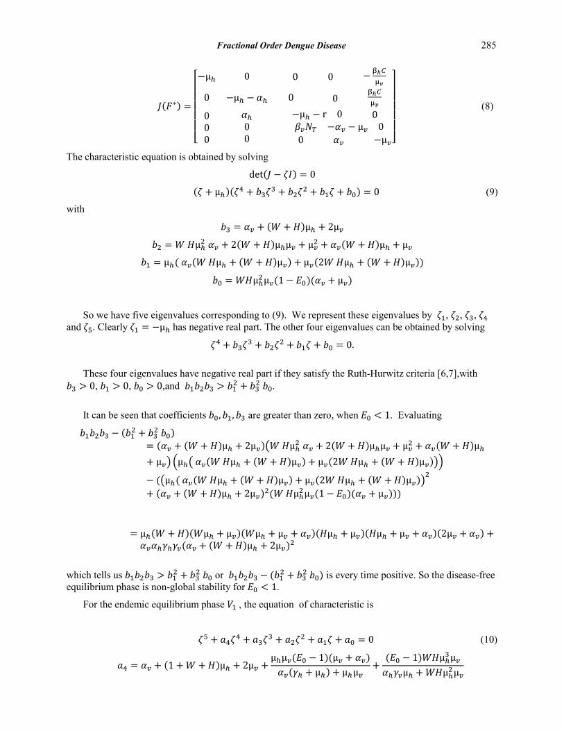
For the equilibrium phase 𝑉𝑉0 = (1, 0, 0,0,0)

Equation (6) reduces to


𝐽𝐽(𝐹𝐹∗) =

⎣⎢⎢⎢⎢⎢⎡−µℎ 0 0 0 −βℎ𝐶𝐶

µ𝑣𝑣

0 −µℎ − 𝛼𝛼ℎ 0 0βℎ𝐶𝐶µ𝑣𝑣

000

𝛼𝛼ℎ00

−µℎ − r 0 0 𝛽𝛽𝑣𝑣𝑁𝑁𝑇𝑇 −𝛼𝛼𝑣𝑣 − µ𝑣𝑣 0

0 𝛼𝛼𝑣𝑣 −µ𝑣𝑣⎦⎥⎥⎥⎥⎥⎤

(8)

The characteristic equation is obtained by solving

det(𝐽𝐽 − 𝜁𝜁𝜁𝜁) = 0

(𝜁𝜁 + µℎ)(𝜁𝜁4 + 𝑏𝑏3𝜁𝜁3 + 𝑏𝑏2𝜁𝜁2 + 𝑏𝑏1𝜁𝜁 + 𝑏𝑏0) = 0 (9)

with

𝑏𝑏3 = 𝛼𝛼𝑣𝑣 + (𝑊𝑊 + 𝐻𝐻)µℎ + 2µ𝑣𝑣

𝑏𝑏2 = 𝑊𝑊 𝐻𝐻µℎ2 𝛼𝛼𝑣𝑣 + 2(𝑊𝑊 + 𝐻𝐻)µℎµ𝑣𝑣 + µ𝑣𝑣2 + 𝛼𝛼𝑣𝑣(𝑊𝑊 + 𝐻𝐻)µℎ + µ𝑣𝑣

𝑏𝑏1 = µℎ( 𝛼𝛼𝑣𝑣(𝑊𝑊 𝐻𝐻µℎ + (𝑊𝑊 +𝐻𝐻)µ𝑣𝑣) + µ𝑣𝑣(2𝑊𝑊 𝐻𝐻µℎ + (𝑊𝑊 + 𝐻𝐻)µ𝑣𝑣))

𝑏𝑏0 = 𝑊𝑊𝐻𝐻µℎ2µ𝑣𝑣(1− 𝐸𝐸0)(𝛼𝛼𝑣𝑣 + µ𝑣𝑣)

So we have five eigenvalues corresponding to (9). We represent these eigenvalues by 𝜁𝜁1, 𝜁𝜁2, 𝜁𝜁3, 𝜁𝜁4 and 𝜁𝜁5. Clearly 𝜁𝜁1 = −µℎ has negative real part. The other four eigenvalues can be obtained by solving

𝜁𝜁4 + 𝑏𝑏3𝜁𝜁3 + 𝑏𝑏2𝜁𝜁2 + 𝑏𝑏1𝜁𝜁 + 𝑏𝑏0 = 0.

These four eigenvalues have negative real part if they satisfy the Ruth-Hurwitz criteria [6,7],with 𝑏𝑏3 > 0, 𝑏𝑏1 > 0, 𝑏𝑏0 > 0,and 𝑏𝑏1𝑏𝑏2𝑏𝑏3 > 𝑏𝑏12 + 𝑏𝑏32 𝑏𝑏0.

It can be seen that coefficients 𝑏𝑏0,𝑏𝑏1,𝑏𝑏3 are greater than zero, when 𝐸𝐸0 < 1. Evaluating

𝑏𝑏1𝑏𝑏2𝑏𝑏3 − (𝑏𝑏12 + 𝑏𝑏32 𝑏𝑏0)= (𝛼𝛼𝑣𝑣 + (𝑊𝑊 + 𝐻𝐻)µℎ + 2µ𝑣𝑣)�𝑊𝑊 𝐻𝐻µℎ2 𝛼𝛼𝑣𝑣 + 2(𝑊𝑊 + 𝐻𝐻)µℎµ𝑣𝑣 + µ𝑣𝑣2 + 𝛼𝛼𝑣𝑣(𝑊𝑊 + 𝐻𝐻)µℎ+ µ𝑣𝑣� �µℎ� 𝛼𝛼𝑣𝑣(𝑊𝑊 𝐻𝐻µℎ + (𝑊𝑊 + 𝐻𝐻)µ𝑣𝑣) + µ𝑣𝑣(2𝑊𝑊 𝐻𝐻µℎ + (𝑊𝑊 + 𝐻𝐻)µ𝑣𝑣)��

− (�µℎ( 𝛼𝛼𝑣𝑣(𝑊𝑊 𝐻𝐻µℎ + (𝑊𝑊 + 𝐻𝐻)µ𝑣𝑣) + µ𝑣𝑣(2𝑊𝑊 𝐻𝐻µℎ + (𝑊𝑊 +𝐻𝐻)µ𝑣𝑣)�2

+ (𝛼𝛼𝑣𝑣 + (𝑊𝑊 +𝐻𝐻)µℎ + 2µ𝑣𝑣)2(𝑊𝑊 𝐻𝐻µℎ2µ𝑣𝑣(1− 𝐸𝐸0)(𝛼𝛼𝑣𝑣 + µ𝑣𝑣)))

= µℎ(𝑊𝑊 + 𝐻𝐻)(𝑊𝑊µℎ + µ𝑣𝑣)(𝑊𝑊µℎ + µ𝑣𝑣 + 𝛼𝛼𝑣𝑣)(𝐻𝐻µℎ + µ𝑣𝑣)(𝐻𝐻µℎ + µ𝑣𝑣 + 𝛼𝛼𝑣𝑣)(2µ𝑣𝑣 + 𝛼𝛼𝑣𝑣) + 𝛼𝛼𝑣𝑣𝛼𝛼ℎ𝛾𝛾ℎ𝛾𝛾𝑣𝑣(𝛼𝛼𝑣𝑣 + (𝑊𝑊 + 𝐻𝐻)µℎ + 2µ𝑣𝑣)2

which tells us 𝑏𝑏1𝑏𝑏2𝑏𝑏3 > 𝑏𝑏12 + 𝑏𝑏32 𝑏𝑏0 or 𝑏𝑏1𝑏𝑏2𝑏𝑏3 − (𝑏𝑏12 + 𝑏𝑏32 𝑏𝑏0) is every time positive. So the disease-free equilibrium phase is non-global stability for 𝐸𝐸0 < 1.

For the endemic equilibrium phase 𝑉𝑉1 , the equation of characteristic is

𝜁𝜁5 + 𝑎𝑎4𝜁𝜁4 + 𝑎𝑎3𝜁𝜁3 + 𝑎𝑎2𝜁𝜁2 + 𝑎𝑎1𝜁𝜁 + 𝑎𝑎0 = 0 (10)

𝑎𝑎4 = 𝛼𝛼𝑣𝑣 + (1 + 𝑊𝑊 +𝐻𝐻)µℎ + 2µ𝑣𝑣 +µℎµ𝑣𝑣(𝐸𝐸0 − 1)(µ𝑣𝑣 + 𝛼𝛼𝑣𝑣)𝛼𝛼𝑣𝑣(𝛾𝛾ℎ + µℎ) + µℎµ𝑣𝑣

+(𝐸𝐸0 − 1)𝑊𝑊𝐻𝐻µℎ3µ𝑣𝑣𝛼𝛼ℎ𝛾𝛾𝑣𝑣µℎ + 𝑊𝑊𝐻𝐻µℎ2µ𝑣𝑣


𝑎𝑎3 = µ𝑣𝑣2 + µℎµ𝑣𝑣 �2(1 +𝑊𝑊 + 𝐻𝐻) +µ𝑣𝑣(𝐸𝐸0 − 1)(µ𝑣𝑣 + 𝛼𝛼𝑣𝑣)𝛼𝛼𝑣𝑣(𝛾𝛾ℎ + µℎ) + µℎµ𝑣𝑣

�

+ µℎ2 �𝑊𝑊 + 𝐻𝐻 + 𝑊𝑊𝐻𝐻 +µ𝑣𝑣(1 + 𝑊𝑊 + 𝐻𝐻)(𝐸𝐸0 − 1)(µ𝑣𝑣 + 𝛼𝛼𝑣𝑣)

𝛼𝛼𝑣𝑣(𝛾𝛾ℎ + µℎ) + µℎµ𝑣𝑣�

+(𝐸𝐸0 − 1)𝑊𝑊𝐻𝐻µℎ3µ𝑣𝑣{(𝑊𝑊 + 𝐻𝐻)µℎ + 2µ𝑣𝑣}

𝛼𝛼ℎ𝛾𝛾𝑣𝑣µℎ + 𝑊𝑊𝐻𝐻µℎ2µ𝑣𝑣

+µℎµ𝑣𝑣(𝐸𝐸0 − 1)(µ𝑣𝑣 + 𝛼𝛼𝑣𝑣)

(𝛼𝛼ℎ𝛾𝛾𝑣𝑣µℎ + 𝑊𝑊𝐻𝐻µℎ2µ𝑣𝑣)(𝛼𝛼𝑣𝑣(𝛾𝛾ℎ + µℎ) + µℎµ𝑣𝑣)

+ �(1 + 𝑊𝑊 +𝐻𝐻)µℎ + µ𝑣𝑣 +µℎµ𝑣𝑣(𝐸𝐸0 − 1)(µ𝑣𝑣 + 𝛼𝛼𝑣𝑣)𝛼𝛼𝑣𝑣(𝛾𝛾ℎ + µℎ) + µℎµ𝑣𝑣

+(𝐸𝐸0 − 1)𝑊𝑊𝐻𝐻µℎ3µ𝑣𝑣𝛼𝛼ℎ𝛾𝛾𝑣𝑣µℎ + 𝑊𝑊𝐻𝐻µℎ2µ𝑣𝑣

�𝛼𝛼𝑣𝑣

𝑎𝑎2 = µℎ

⎩⎪⎨

⎪⎧𝑊𝑊𝐻𝐻µℎ2 + 2(𝑊𝑊𝐻𝐻 + 𝑊𝑊 + 𝐻𝐻)µℎµ𝑣𝑣 + (1 + 𝑊𝑊 + 𝐻𝐻)µ𝑣𝑣2

+µℎµ𝑣𝑣(𝐸𝐸0 − 1)(µ𝑣𝑣 + 𝛼𝛼𝑣𝑣)�(𝑊𝑊 + 𝐻𝐻 + 𝑊𝑊𝐻𝐻)µℎ + (1 + 𝑊𝑊 + 𝐻𝐻)µ𝑣𝑣�

𝛼𝛼𝑣𝑣(𝛾𝛾ℎ + µℎ) + µℎµ𝑣𝑣

+𝑊𝑊𝐻𝐻µℎ2µ𝑣𝑣(𝐸𝐸0 − 1)�𝑊𝑊𝐻𝐻µℎ2 + 2(𝑊𝑊 + 𝐻𝐻)µℎµ𝑣𝑣 + µ𝑣𝑣2�


+𝑊𝑊𝐻𝐻µℎ2µ𝑣𝑣(𝐸𝐸0 − 1) �µℎµ𝑣𝑣(𝐸𝐸0 − 1)(µ𝑣𝑣 + 𝛼𝛼𝑣𝑣)((𝑊𝑊 + 𝐻𝐻)µℎ + µ𝑣𝑣)



+ 𝛼𝛼𝑣𝑣 �(𝑊𝑊𝐻𝐻 + 𝑊𝑊 + 𝐻𝐻)µℎ + (1 + 𝑊𝑊 + 𝐻𝐻)µ𝑣𝑣

+µ𝑣𝑣µℎ(1 + 𝑊𝑊 + 𝐻𝐻)(𝐸𝐸0 − 1)(µ𝑣𝑣 + 𝛼𝛼𝑣𝑣)


+𝑊𝑊𝐻𝐻µℎ2µ𝑣𝑣(𝐸𝐸0 − 1) �(𝑊𝑊 + 𝐻𝐻)µℎ + µ𝑣𝑣 + µℎµ𝑣𝑣(𝐸𝐸0 − 1)(µ𝑣𝑣 + 𝛼𝛼𝑣𝑣)


𝛼𝛼ℎ𝛾𝛾𝑣𝑣µℎ +𝑊𝑊𝐻𝐻µℎ2µ𝑣𝑣�

⎭⎪⎬

⎪⎫


𝑎𝑎1 = µℎ2

⎩⎪⎨

⎪⎧µℎ2µ𝑣𝑣𝑊𝑊𝑊𝑊(𝐸𝐸0 − 1)(µ𝑣𝑣 + 𝛼𝛼𝑣𝑣)�1 + 𝑊𝑊(𝐸𝐸0 − 1)µℎ2µ𝑣𝑣

𝛼𝛼ℎ𝛾𝛾𝑣𝑣µℎ + 𝑊𝑊µℎ2µ𝑣𝑣�


+ µ𝑣𝑣2 �𝑊𝑊 + 𝑊𝑊 + 𝑊𝑊𝑊𝑊 +𝑊𝑊(𝑊𝑊 + 𝑊𝑊)(𝐸𝐸0 − 1)µℎ2µ𝑣𝑣


+ µ𝑣𝑣µℎ �2𝑊𝑊𝑊𝑊 +µ𝑣𝑣(𝑊𝑊𝑊𝑊 +𝑊𝑊 + 𝑊𝑊)(𝐸𝐸0 − 1)(µ𝑣𝑣 + 𝛼𝛼𝑣𝑣)


+𝑊𝑊µℎ2µ𝑣𝑣(𝐸𝐸0 − 1) �2𝑊𝑊𝑊𝑊 + µ𝑣𝑣(𝐸𝐸0 − 1)(𝑊𝑊 + 𝑊𝑊)(µ𝑣𝑣 + 𝛼𝛼𝑣𝑣)


𝛼𝛼ℎ𝛾𝛾𝑣𝑣µℎ +𝑊𝑊µℎ2µ𝑣𝑣�

+ 𝛼𝛼𝑣𝑣 �𝑊𝑊𝑊𝑊µℎ + (𝑊𝑊 + 𝑊𝑊 + 𝑊𝑊𝑊𝑊)µ𝑣𝑣 +µℎµ𝑣𝑣(𝐸𝐸0 − 1)(𝑊𝑊 + 𝑊𝑊 + 𝑊𝑊𝑊𝑊)(µ𝑣𝑣 + 𝛼𝛼𝑣𝑣)


+𝑊𝑊µℎ2µ𝑣𝑣(𝐸𝐸0 − 1) �𝑊𝑊𝑊𝑊µℎ + (𝑊𝑊 + 𝑊𝑊)µ𝑣𝑣 + µℎµ𝑣𝑣(𝐸𝐸0 − 1)(𝑊𝑊 + 𝑊𝑊)(µ𝑣𝑣 + 𝛼𝛼𝑣𝑣)



⎭⎪⎬

⎪⎫

𝑎𝑎0 = (µ𝑣𝑣 + 𝛼𝛼𝑣𝑣)µℎµ𝑣𝑣 �𝑊𝑊𝑊𝑊µℎ2 �1 +𝑊𝑊(𝐸𝐸0 − 1)µℎ2µ𝑣𝑣𝛼𝛼ℎ𝛾𝛾𝑣𝑣µℎ + 𝑊𝑊µℎ2µ𝑣𝑣

��1 +µℎ(𝐸𝐸0 − 1)(µ𝑣𝑣 + 𝛼𝛼𝑣𝑣)𝛼𝛼𝑣𝑣(𝛾𝛾ℎ + µℎ) + µℎµ𝑣𝑣

��

Equation (10) corresponds five eigenvalues. We represent these five eigenvalues by 𝜁𝜁1, 𝜁𝜁2, 𝜁𝜁3, 𝜁𝜁4 and 𝜁𝜁5. These five eigenvalues have negative real parts if they satisfy the Routh-Hurwitz criteria [6, 7], that is,

𝑎𝑎𝑖𝑖 > 0, for 𝑖𝑖 = 0,1,2,3,4

𝑎𝑎2𝑎𝑎3𝑎𝑎4 > 𝑎𝑎22 + 𝑎𝑎42 𝑎𝑎1

(𝑎𝑎1𝑎𝑎4 − 𝑎𝑎0)(𝑎𝑎4𝑎𝑎3𝑎𝑎2 − 𝑎𝑎22 − 𝑎𝑎42 𝑎𝑎1) > 𝑎𝑎0(𝑎𝑎4𝑎𝑎3 − 𝑎𝑎2)2 + 𝑎𝑎4𝑎𝑎02

If all these conditions satisfy and will satisfy (already checked) for 𝐸𝐸0 > 1. Thus, the endemic equilibrium phase is non-global stability for 𝐸𝐸0 > 1.

5. NSFD DISCRETIZATION FOR FRACTIONAL-ORDER DENGUE MODEL

In this section we shall construct Non Standard Finite Difference Scheme proposed by Mickens [2, 13], for the system (4) and swapping the step size ℎ by a function 𝜓𝜓(ℎ) and using GL discretization technique, it can be seen that

∑ 𝐶𝐶𝑗𝑗𝛾𝛾1 𝑆𝑆𝑛𝑛+1−𝑗𝑗𝑛𝑛+1

𝑗𝑗=0 = µℎ − 𝛽𝛽ℎS𝑛𝑛+1𝐼𝐼𝑣𝑣𝑛𝑛 � Cµ𝑣𝑣� − µℎS𝑛𝑛+1 (11)


∑ 𝐶𝐶𝑗𝑗𝛾𝛾2 𝑋𝑋𝑛𝑛+1−𝑗𝑗𝑛𝑛+1

𝑗𝑗=0 = βℎS𝑛𝑛+1𝐼𝐼𝑣𝑣𝑛𝑛 � Cµ𝑣𝑣� − 𝛼𝛼ℎ𝑋𝑋𝑛𝑛+1 − µℎ𝑋𝑋𝑛𝑛+1 (12)

∑ 𝐶𝐶𝑗𝑗𝛾𝛾3 𝐼𝐼𝑛𝑛+1−𝑗𝑗𝑛𝑛+1

𝑗𝑗=0 = 𝛼𝛼ℎ𝑋𝑋𝑛𝑛+1 − 𝑟𝑟𝐼𝐼𝑛𝑛+1 − µℎ𝐼𝐼𝑛𝑛+1 (13)

∑ 𝐶𝐶𝑗𝑗𝛾𝛾4 𝑋𝑋𝑣𝑣𝑛𝑛+1−𝑗𝑗𝑛𝑛+1

𝑗𝑗=0 = 𝛽𝛽𝑣𝑣𝐼𝐼𝑛𝑛+1𝑁𝑁𝑇𝑇(1 − 𝑋𝑋𝑣𝑣𝑛𝑛+1 − 𝐼𝐼𝑣𝑣𝑛𝑛) − 𝛼𝛼𝑣𝑣𝑋𝑋𝑣𝑣𝑛𝑛+1 − µ𝑣𝑣𝑋𝑋𝑣𝑣𝑛𝑛+1 (14)

∑ 𝐶𝐶𝑗𝑗𝛾𝛾5 𝐼𝐼𝑣𝑣𝑛𝑛+1−𝑗𝑗𝑛𝑛+1

𝑗𝑗=0 = 𝛼𝛼𝑣𝑣𝑋𝑋𝑣𝑣𝑛𝑛+1 − µ𝑣𝑣𝐼𝐼𝑣𝑣𝑛𝑛+1 (15)

(11) ⟹ 𝑆𝑆𝑛𝑛+1 =µℎ −∑ 𝐶𝐶𝑗𝑗

𝛾𝛾1 𝑆𝑆𝑛𝑛+1−𝑗𝑗𝑛𝑛+1𝑗𝑗=1

(𝐶𝐶0𝛾𝛾1+𝛽𝛽ℎ𝐼𝐼𝑣𝑣𝑛𝑛 � Cµ𝑣𝑣

�+µℎ) (16)

(12) ⟹ 𝑋𝑋𝑛𝑛+1 =βℎS𝑛𝑛+1𝐼𝐼𝑣𝑣𝑛𝑛 � Cµ𝑣𝑣

�−∑ 𝐶𝐶𝑗𝑗𝛾𝛾2 𝑋𝑋𝑛𝑛+1−𝑗𝑗𝑛𝑛+1

𝑗𝑗=1

𝐶𝐶0𝛾𝛾2+𝛼𝛼ℎ+µℎ

(17)

(13) ⟹ 𝐼𝐼𝑛𝑛+1 =𝛼𝛼ℎ𝑋𝑋𝑛𝑛+1−∑ 𝐶𝐶𝑗𝑗

𝛾𝛾3 𝐼𝐼𝑛𝑛+1−𝑗𝑗𝑛𝑛+1𝑗𝑗=1

𝐶𝐶0𝛾𝛾3+𝑟𝑟+µℎ

(18)

(14) ⟹ 𝑋𝑋𝑣𝑣𝑛𝑛+1 =𝛽𝛽𝑣𝑣𝐼𝐼𝑛𝑛+1𝑁𝑁𝑇𝑇−𝛽𝛽𝑣𝑣𝐼𝐼𝑛𝑛+1𝑁𝑁𝑇𝑇𝐼𝐼𝑣𝑣𝑛𝑛−∑ 𝐶𝐶𝑗𝑗

𝛾𝛾4 𝑋𝑋𝑣𝑣𝑛𝑛+1−𝑗𝑗𝑛𝑛+1𝑗𝑗=1

𝐶𝐶0𝛾𝛾4+𝛽𝛽𝑣𝑣𝐼𝐼𝑛𝑛+1𝑁𝑁𝑇𝑇+𝛼𝛼𝑣𝑣+µ𝑣𝑣

(19)

(15) ⟹ 𝐼𝐼𝑣𝑣𝑛𝑛+1 =𝛼𝛼𝑣𝑣𝑋𝑋𝑣𝑣𝑛𝑛+1−∑ 𝐶𝐶𝑗𝑗

𝛾𝛾5 𝐼𝐼𝑣𝑣𝑛𝑛+1−𝑗𝑗𝑛𝑛+1𝑗𝑗=1

𝐶𝐶0𝛾𝛾5+µ𝑣𝑣

(20)

with 𝐶𝐶0𝑛𝑛1 = �𝑒𝑒

µℎℎ−1µℎ

�−𝛾𝛾1

, 𝐶𝐶0𝑛𝑛2 = �𝑒𝑒

(𝛼𝛼ℎ+µℎ)ℎ−1(𝛼𝛼ℎ+µℎ)

�−𝛾𝛾2

, 𝐶𝐶0𝑛𝑛3 = �𝑒𝑒

(𝑟𝑟+µℎ)ℎ−1𝑟𝑟+µℎ

�−𝛾𝛾3

,

𝐶𝐶0𝑛𝑛4 = �𝑒𝑒

(𝛼𝛼ℎ+µℎ)ℎ−1(𝛼𝛼ℎ+µℎ)

�−𝛾𝛾4

and 𝐶𝐶0𝑛𝑛5 = �𝑒𝑒

µ𝑣𝑣ℎ−1µ𝑣𝑣

�−𝛾𝛾5

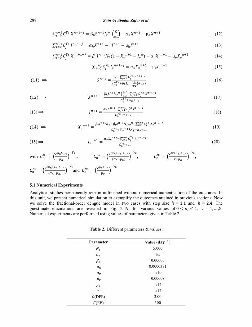
5.1 Numerical Experiments

Analytical studies permanently remain unfinished without numerical authentication of the outcomes. In this unit, we present numerical simulation to exemplify the outcomes attained in previous sections. Now we solve the fractional-order dengue model in two cases with step size ℎ = 1.1 and ℎ = 2.4. The guestimate elucidations are revealed in Fig. 2-19, for various values of 0 < 𝑛𝑛𝑖𝑖 ≤ 1, 𝑖𝑖 = 1, … ,5. Numerical experiments are performed using values of parameters given in Table 2.

Table 2. Different parameters & values.

Parameter Value (𝐝𝐝𝐝𝐝𝐝𝐝−𝟏𝟏) 𝑁𝑁𝑇𝑇 5,000 𝛼𝛼ℎ 1/5 𝛽𝛽ℎ 0.00005 𝜇𝜇ℎ 0.0000391 𝛼𝛼𝑣𝑣 1/10 𝛽𝛽𝑣𝑣 0.00008 𝜇𝜇𝑣𝑣 1/14 𝑟𝑟 1/14

𝐶𝐶(DFE) 3.00 𝐶𝐶(EE) 300


6. RESULTS AND DISCUSSION

The numerical modeling of transmission dynamics of Fractional Order dengue disease with incubation period of virus has been analysed in this paper. The model has two equilibrium points, i.e. disease free equilibrium (DFE) and endemic equilibrium (EE). An unconditionally convergent non-standard finite difference numerical model with GL coefficients has been constructed and numerical experiments are performed for different values of discretization parameter ℎ. Fig. (2-10) shows the graphs of disease free equilibrium with step size ℎ = 1.1 and Fig. (11-19) with step size ℎ = 2.4. Numerical Simulations reveals that all values approaches to equilibrium point. In order to observe the effects that the parameter 𝛾𝛾 has on the dynamics of the fractional-order model (4), we conclude several numerical simulations varying the value of parameter. These simulations reveal that a change of the value 𝛾𝛾 affects the dynamics of the epidemic. For example, Fig. 2, 11 shows that for lower values of 𝛾𝛾, the epidemic peak is wider and lower from the true equilibrium points, Fig. 4, 6, 8, 10, 13, 15, 17, and 19 show that for lower values of 𝛾𝛾, the epidemic peak is wider and higher for true equilibria. This feature is important from an epidemiological point of view since its interpretation shows a longer period in which infected & infectious individuals can affect the health system. Fig. 2-19 show that the model presented here gradually approaches the steady state for different values of 𝛾𝛾 but the dynamics of the model is governed by the distinct paths.

Fig.1. Flow diagram.

Fig. 2. The susceptible humans for different values of 𝛾𝛾 ’𝑠𝑠 with ℎ = 1.1.

0 1 2 3 4 5 6 7x 104

0

0.2

0.4

0.6

0.8

1

Time

Susc

eptib

le S

(t)

Susceptible Human

γ1=γ2=γ3=γ4=γ5=0.6

γ1=γ2=γ3=γ4=γ5=0.7

γ1=γ2=γ3=γ4=γ5=0.8

γ1=γ2=γ3=γ4=γ5=0.9

γ1=γ2=γ3=γ4=γ5=1

0.9556

0.6264

0.2859

0.10760.03715

𝛼𝛼ℎ𝑋𝑋�ℎ 𝛽𝛽ℎ𝑆𝑆ℎ̅𝐼𝐼�̅�𝑣

µℎ𝑅𝑅�ℎ µℎ𝑆𝑆ℎ̅ µℎ𝐼𝐼ℎ̅ µℎ𝑋𝑋�ℎ

𝑟𝑟𝐼𝐼ℎ̅ 𝑅𝑅�ℎ 𝑋𝑋�ℎ 𝐼𝐼ℎ̅

α𝑣𝑣𝑋𝑋�𝑣𝑣

µ𝑣𝑣𝑋𝑋�𝑣𝑣

𝛽𝛽𝑣𝑣𝐼𝐼ℎ̅�̅�𝑆𝑣𝑣

µ𝑣𝑣𝑆𝑆�̅�𝑣 µ𝑣𝑣𝐼𝐼�̅�𝑣

𝑋𝑋�𝑣𝑣 𝐶𝐶

𝑆𝑆�̅�𝑣 𝐼𝐼�̅�𝑣

𝜆𝜆𝑁𝑁𝑇𝑇 𝑆𝑆ℎ̅


Fig. 3. The infected humans for different values of 𝛾𝛾 ’𝑠𝑠 with ℎ = 1.1.

Fig. 4. The infected humans, in zoom.

Fig. 5. The infectious humans for different values of 𝛾𝛾 ’𝑠𝑠 with ℎ = 1.1.

0 1 2 3 4 5 6 7x 104

0

1

2

3

4

5

6

7

8

9 x 10-5

Time

Infe

cted

X(t)

Infected Human

γ1=γ2=γ3=γ4=γ5=0.6

γ1=γ2=γ3=γ4=γ5=0.7

γ1=γ2=γ3=γ4=γ5=0.8

γ1=γ2=γ3=γ4=γ5=0.9

γ1=γ2=γ3=γ4=γ5=1

7.0001 7.0001 7.0001 7.0001 7.0001 7.0001x 104

0

1

2

3

4

5

6

7x 10-11

Time

Infe

cted

X(t)

Infected Human

γ1=γ2=γ3=γ4=γ5=1

γ1=γ2=γ3=γ4=γ5=0.9

γ1=γ2=γ3=γ4=γ5=0.8

γ1=γ2=γ3=γ4=γ5=0.7

γ1=γ2=γ3=γ4=γ5=0.6

9.881e-324

1.204e-011

3.139e-011

6.761e-011

5.098e-011

0 1 2 3 4 5 6 7x 104

0

2

4

6

8

10

12

14

x 10-5

Time

Infe

ctio

us I(

t)

Infectious Human

γ1=γ2=γ3=γ4=γ5=1

γ1=γ2=γ3=γ4=γ5=0.9

γ1=γ2=γ3=γ4=γ5=0.8

γ1=γ2=γ3=γ4=γ5=0.7

γ1=γ2=γ3=γ4=γ5=0.6


Fig. 6. The infectious humans, in zoom.

Fig. 7. The graph of infected mosquitoes for different values of 𝛾𝛾 ’𝑠𝑠 with ℎ = 1.1.

Fig. 8. The infected mosquitoes, in zoom.

7.0001 7.0001 7.0001 7.0001 7.0001 7.0001 7.0001 7.0001 7.0001 7.0001 7.0001x 104

0

0.5

1

1.5

2

2.5

x 10-10

Time

Infe

ctio

us I(

t)Infectious Human

γ1=γ2=γ3=γ4=γ5=1

γ1=γ2=γ3=γ4=γ5=0.9

γ1=γ2=γ3=γ4=γ5=0.8

γ1=γ2=γ3=γ4=γ5=0.7

γ1=γ2=γ3=γ4=γ5=0.6

3.683e-011

5.435e-323

1.003e-010

1.763e-010

2.623e-010

0 1 2 3 4 5 6 7 8x 104

0

0.02

0.04

0.06

0.08

0.1

Time

Infe

cted

Xv(

t)

Infected Mosquitos

γ1=γ2=γ3=γ4=γ5=1

γ1=γ2=γ3=γ4=γ5=0.9

γ1=γ2=γ3=γ4=γ5=0.8

γ1=γ2=γ3=γ4=γ5=0.7

γ1=γ2=γ3=γ4=γ5=0.6

7.0001 7.0001 7.0001 7.0001 7.0001 7.0001x 104

0

5

10

15x 10-9

Time

Infe

cted

Xv(

t)

Infected Mosquitos

γ1=γ2=γ3=γ4=γ5=1

γ1=γ2=γ3=γ4=γ5=0.9

γ1=γ2=γ3=γ4=γ5=0.8

γ1=γ2=γ3=γ4=γ5=0.7

γ1=γ2=γ3=γ4=γ5=0.6

1.186e-3222.296e-0101.098e-009

4.162e-009

1.456e-008


Fig. 9. The infectious mosquitoes for different values of 𝛾𝛾 ’𝑠𝑠 with ℎ = 1.1.

Fig. 10. The infectious mosquitoes in zoom.

Fig. 11. The susceptible humans for different values of 𝛾𝛾 ’𝑠𝑠 with ℎ = 2.4.

0 1 2 3 4 5 6 7x 104

0

0.02

0.04

0.06

0.08

0.1

0.12

Time

Infe

ctio

us Iv

(t)Infectious Mosquitos

γ1=γ2=γ3=γ4=γ5=1

γ1=γ2=γ3=γ4=γ5=0.9

γ1=γ2=γ3=γ4=γ5=0.8

γ1=γ2=γ3=γ4=γ5=0.7

γ1=γ2=γ3=γ4=γ5=0.6

7.0001 7.0001 7.0001 7.0001 7.0001 7.0001 7.0001x 104

0

2

4

6

8

10

12

14

16x 10-8

Time

Infe

ctio

us Iv

(t)

Infectious Mosquitos

γ1=γ2=γ3=γ4=γ5=1

γ1=γ2=γ3=γ4=γ5=0.9

γ1=γ2=γ3=γ4=γ5=0.8

γ1=γ2=γ3=γ4=γ5=0.7

γ1=γ2=γ3=γ4=γ5=0.6

1.729e-3221.729e-322

1.507e-007

4.154e-008

9.962e-0091.774e-009

0 1 2 3 4 5 6 7x 104

0

0.2

0.4

0.6

0.8

1

Time

Susc

eptib

le S

(t)

Susceptible Human

γ1=γ2=γ3=γ4=γ5=1

γ1=0.9,γ2=0.8,γ3=0.7,γ4=0.6,γ5=0.5

γ1=0.66,γ2=0.62,γ3=0.58,γ4=0.56,γ5=0.54

γ1=0.57,γ2=0.55,γ3=0.53,γ4=0.51,γ5=0.49

γ1=0.45,γ2=0.43,γ3=0.41,γ4=0.39,γ5=0.37

0.009940.04098

0.1135

0.8356

0.9987


Fig. 12. The infected humans for different values of 𝛾𝛾 ’𝑠𝑠 with ℎ = 2.4.

Fig. 13. The infected humans, in zoom.

Fig. 14. The infectious humans for different values of 𝛾𝛾 ’𝑠𝑠 with ℎ = 2.4.

0 1 2 3 4 5 6 7x 104

0

0.2

0.4

0.6

0.8

1 x 10-4

Time

Infe

cted

X(t)

Infected Human

γ1=γ2=γ3=γ4=γ5=1

γ1=0.9,γ2=0.8,γ3=0.7,γ4=0.6,γ5=0.5

γ1=0.66,γ2=0.62,γ3=0.58,γ4=0.56,γ5=0.54

γ1=0.57,γ2=0.55,γ3=0.53,γ4=0.51,γ5=0.49

γ1=0.45,γ2=0.43,γ3=0.41,γ4=0.39,γ5=0.37

7.0001 7.0001 7.0001 7.0001 7.0001 7.0001 7.0001x 104

-1

0

1

2

3

4

5

x 10-11

Time

Infe

cted

X(t)

Infected Human

γ1=γ2=γ3=γ4=γ5=1

γ1=0.9,γ2=0.8,γ3=0.7,γ4=0.6,γ5=0.5

γ1=0.66,γ2=0.62,γ3=0.58,γ4=0.56,γ5=0.54

γ1=0.57,γ2=0.55,γ3=0.53,γ4=0.51,γ5=0.49

γ1=0.45,γ2=0.43,γ3=0.41,γ4=0.39,γ5=0.37

4.96e-0114.626e-011

3.913e-011

1.695e-011

9.881e-324

0 1 2 3 4 5 6 7x 104

0

0.5

1

1.5 x 10-4

Time

Infe

ctio

us I(

t)

Infectious Human

γ1=γ2=γ3=γ4=γ5=1

γ1=0.9,γ2=0.8,γ3=0.7,γ4=0.6,γ5=0.5

γ1=0.66,γ2=0.62,γ3=0.58,γ4=0.56,γ5=0.54

γ1=0.57,γ2=0.55,γ3=0.53,γ4=0.51,γ5=0.49

γ1=0.45,γ2=0.43,γ3=0.41,γ4=0.39,γ5=0.37


Fig. 15. The infectious humans, in zoom.

Fig. 16. The infected mosquitoes for different values of 𝛾𝛾 ’𝑠𝑠 with ℎ = 2.4.

Fig. 17. The infected mosquitoes, in zoom.

7.0001 7.0001 7.0001 7.0001 7.0001 7.0001x 104

0

0.5

1

1.5

2

2.5

x 10-10

Time

Infe

ctio

us I(

t)

Infectious Human

γ1=γ2=γ3=γ4=γ5=1

γ1=0.9,γ2=0.8,γ3=0.7,γ4=0.6,γ5=0.5

γ1=0.66,γ2=0.62,γ3=0.58,γ4=0.56,γ5=0.54

γ1=0.57,γ2=0.55,γ3=0.53,γ4=0.51,γ5=0.49

γ1=0.45,γ2=0.43,γ3=0.41,γ4=0.39,γ5=0.37

3.458e-323

5.823e-011

1.688e-010

1.836e-010

2.514e-010

0 1 2 3 4 5 6 7x 104

0

0.02

0.04

0.06

0.08

0.1

Time

Infe

cted

Xv(

t)

Infected Mosquitos

γ1=γ2=γ3=γ4=γ5=1

γ1=0.9,γ2=0.8,γ3=0.7,γ4=0.6,γ5=0.5

γ1=0.66,γ2=0.62,γ3=0.58,γ4=0.56,γ5=0.54

γ1=0.57,γ2=0.55,γ3=0.53,γ4=0.51,γ5=0.49

γ1=0.45,γ2=0.43,γ3=0.41,γ4=0.39,γ5=0.37

7.0001 7.0001 7.0001 7.0001 7.0001 7.0001 7.0001 7.0001 7.0001 7.0001 7.0001x 104

0

0.5

1

1.5

2

2.5

3

3.5

x 10-8

Time

Infe

cted

Xv(

t)

Infected Mosquitos

γ1=γ2=γ3=γ4=γ5=1

γ1=0.9,γ2=0.8,γ3=0.7,γ4=0.6,γ5=0.5

γ1=0.66,γ2=0.62,γ3=0.58,γ4=0.56,γ5=0.54

γ1=0.57,γ2=0.55,γ3=0.53,γ4=0.51,γ5=0.49

γ1=0.45,γ2=0.43,γ3=0.41,γ4=0.39,γ5=0.37

3.784e-008

8.472e-009

3.188e-091.968e-108.893e-323


Fig. 18. The infectious mosquitoes for different values of 𝛾𝛾 ’𝑠𝑠 with ℎ = 2.4.

Fig. 19. The infectious mosquitoes, in zoom.

6. CONCLUSIONS

Describing the reality through a mathematical model, usually a system of differential equations, is hard task that has an inherent compromise between simplicity and accuracy. In this article we studied the fractional-order dengue model. It turns out that, in general, this classical model does not provide enough good results. In order to get better results, that fit the reality, fractional order system is needed. It allows us to model memory effects, and result in a more powerful approach to epidemiological models. Our investigation show that even a simple fractional model may give surprisingly good results. From the obtained results from the presented figures, it turns out that the results are non-negative because susceptible, infected and recovered can never be less than zero. Then the local stability analysis of the model in fractional order is presented. The results obtained are in agreement with the numerical simulations attained from the graph.

7. REFERENCES

1. Yıldırım, A. & Y. Cherruault. Analytical approximate solution of a SIR epidemic model with constant vaccination strategy by homotopy perturbation method. Kybernetes 38(9): 1566-1575 (2009).

2. Makinde, O.D. Adomian decomposition approach to a SIR epidemic model with constant vaccination strategy. Applied Mathematics & Computation 184(2): 842-848 (2007).

3. Arafa, A.A.M., S.Z. Rida & M. Khalil. Fractional modeling dynamics of HIV and 4 T-cells during primary Infection. Nonlinear Biomedical Physics 6: 1-7 (2012).

0 1 2 3 4 5 6 7 8x 104

0

0.02

0.04

0.06

0.08

0.1

Time

Infe

ctio

us M

osqu

itos

Iv(t)

Infectious Mosquitoes

γ1=γ2=γ3=γ4=γ5=1

γ1=0.9,γ2=0.8,γ3=0.7,γ4=0.6,γ5=0.5

γ1=0.66,γ2=0.62,γ3=0.58,γ4=0.56,γ5=0.54

γ1=0.57,γ2=0.55,γ3=0.53,γ4=0.51,γ5=0.49

γ1=0.45,γ2=0.43,γ3=0.41,γ4=0.39,γ5=0.37

7 7 7 7 7 7 7 7 7 7 7x 104

0

0.5

1

1.5

2

2.5

3

x 10-7

Time

Infe

ctio

us M

osqu

itos

Iv(t)

Infectious Mosquitoes

γ1=γ2=γ3=γ4=γ5=1

γ1=0.9,γ2=0.8,γ3=0.7,γ4=0.6,γ5=0.5

γ1=0.66,γ2=0.62,γ3=0.58,γ4=0.56,γ5=0.54

γ1=0.57,γ2=0.55,γ3=0.53,γ4=0.51,γ5=0.49

γ1=0.45,γ2=0.43,γ3=0.41,γ4=0.39,γ5=0.37

1.63e-322

3.231e-07

7.836e-08

3.899e-08

1.899e-09


4. Hethcote, H.W. The mathematics for infectious diseases, Siam Review 42(4): 599-653 (2000). 5. Biazar, J. Solution of the epidemic model by adomian decomposition method. Applied Mathematics &

Computation 173(2):1101–1106 (2006). 6. Busenberg, S. & P. Driessche. Analysis of a disease transmission model in a population with varying size.

Journal of Mathematical Biology 28:257- 270 (1990). 7. El-Sayed, A.M.A, S.Z. Rida & A.A.M. Arafa. On the solutions of time-fractional bacterial chemotaxis in a

diffusion gradient chamber. International Journal of Nonlinear Science 7: 485-492 (2009). 8. Hassan, H.N. & M.A. El-Tawil. A new technique of using homotopy analysis method for solving high-order

non-linear differential equations. Mathematical Methods in Applied Science 34:728–742(2011). 9. Liao, S.J. A kind of approximate solution technique which does not depend upon small parameters: a special

Example. International Journal of Non-Linear Mechanics 30:371–380 (1995). 10. Liao, S.J. Beyond Perturbation: Introduction to the Homotopy Analysis Method. Chapman & Hall/CRC Press,

Boca Raton (2003). 11. Zibaei, S. & M. Namjoo. A nonstandard finite differnce scheme for solving fractional-order Model of HIV-1

infection of CD4+ T-cells. Iranian Journal of Mathematical Chemistry 6(2): 169-184(2015). 12. Ahmad, E., A.M. Atial, El-Sayed & H.A.A. El-Saka. On some Routh-Hurwitz conditions for fractional order

differential equations and their applications in Lorenz, Rossler, Chua and Chen systems. Physics Letters A 358(1): 1-4 (2006).

13. Mickens, R.E. Calculation of denominator functions for nonstandard finite difference schemes for differential equations satisfying a positivity condition. Numerical Methods of partial Differential Equations 23(3): 672-691 (2007).

14. Matignon, D. Stability result on fractional differential equations with applications to control processing to control processing, In: Computational Engineering in Systems Applications(Conference), p. 963–968 (1996).

15. Zafar, Z., K. Rehan, M. Mushtaq & M. Rafiq. Numerical modelling for nonlinear biochemical reaction networks. Iranian Journal of Mathematical Chemistry (Accepted for publication).

16. Pooseh, S., H.S. Rodrigues, & D.F.M. Torres. Fractional derivatives in dengue epidemics. doi: 10.1063/1.3636838 (2011).

17. Jan, R., & A. Jan. MSGDTM for solution of fractional order dengue disease model. International Journal of Science and Research 6(3): 1140-1144 (2017).

18. Al-Sulami, H., M. El-Shahed, J.J. Nieto, & W. Shammakh. On fractional order dengue epidemic model. Mathematical Problems in Engineering, http://dx.doi.org/10.1155/2014/456537 (2014).

19. Metzler, R., & J. Klafter. The random walk’s guide to anomalous diffusion: a fractional dynamics approach, Physics Reports 339:1-77 (2000).

20. West, B.J., P. Grigolini, & R. Metzler. Nonnenmacher, TF: Fractional diffusion and Le’vy stable processes. Physics Review E. 55(1): 99-106 (1997).

21. Golmankhaneh, A.K., R. Arefi, & D. Baleanu. Synchronization in a nonidentical fractional order of a proposed modified system. Journal of Vibration and Control, 21(6): 1154-1161 (2015).

22. Baleanu, D., A.K. Golmankhaneh, A.K. Golmankhaneh, & R.R. Nigmatullin. Newtonian Law with memory. Nonlinear Dynamics 60: 81-86 (2010).

23. Agila, A., D. Baleanu, R. Eid, & B. Irfanoglu. Applications of the extended fractional euler- lagrange equations model to freely oscillating dynamical systems. Romanian Journal of Physics 61(3-4): 350-359 (2016).

24. Baleanu, D & O.G. Mustafa. On the global existence of solutions to a class of fractional differential equations. Computers & Mathematics with Applications 59: 1835-1841 (2010).

25. He, J, Li, Z, Wang, Q: A new fractional derivative and its application to explanation of polar bear basis. Journal of King Saud University-Science 28:190-192 (2016).

26. Oliveira, E.C., & J.A.T. Machado. A review of definitions for fractional derivatives and Integral. Mathematical Problems in Engineering (2014). http://dx.doi.org/10.1155/2014/238459.

27. Caputo, M, & M. Fabrizio. A new definition of fractional derivative without singular kernel. Progress in Fractional Differentiations and Applications 1(2):73-85 (2015).

28. Atangana, A., & D. Baleanu. New fractional derivatives with non-local and non-singular kernel. Thermal Science 20(2):763-769 (2016).

29. Zafar, Z., K. Rehan, & M. Mushtaq. Fractional-order scheme for bovine babesiosis disease and tick populations. advances in difference equations. p. 86 (2017). http://dx.doi.org/10.1186/s13662-017-1133-2.

30. Zafar, Z., K. Rehan, M. Mushtaq, & M. Rafiq. Numerical Treatment for nonlinear Brusselator Chemical Model. Journal of Difference Equations and Applications 23(3): 521-538 (2017).

31. Zafar, Z., K. Rehan, & M. Mushtaq. HIV/AIDS epidemic fractional-order model. Journal of Difference Equations and Applications 23(7): 1298-1315 (2017).


Documents

Numerical Simulation of Fractional Order Dengue … · Numerical Simulation of Fractional Order Dengue Disease with Incubation Period of Virus Zain Ul Abadin Zafar*1, 3, M. Mushtaq1,